Finite Change Comparative Statics for Risk-Coherent

Inventories

E. Borgonovo� and L. PeccatiEleusi Research Center and Department of Decision SciencesBocconi UniversityVia Roentgen 1, 20135 Milano, Italy

Abstract

This work introduces a comprehensive approach to the sensitivity analysis (SA) of risk-

coherent inventory models. We address the issues posed by i) the piecewise-de�ned nature of

risk-coherent objective functions and ii) by the need of multiple model evaluations. The solutions

of these issues is found by introducing the extended �nite change sensitivity indices (FCSI�s).

We obtain properties and invariance conditions for the sensitivity of risk-coherent optimization

problems. An inventory management case study involving risk-neutral and conditional value-at-

risk (CVaR) objective function illustrates our methodology. Three SA settings are formulated

to obtain managerial insights. Numerical �ndings show that risk-neutral decision-makers are

more exposed to variations in exogenous variables than CVaR decision-makers.

Keywords: Inventory Management; Sensitivity Analysis; Comparative Statics; Finite Change

Sensitivity Indices; Coherent Risk Measures

�emanuele.borgonovo@unibocconi.it

1 Introduction

Recent works have demonstrated the use of coherent measures as a novel and e¤ective way to

manage risk in inventory problems [Ahmed et al (2007), Gotoh and Takano (2007), Borgonovo and

Peccati (2009a)]. The convexity of the objective functions insures feasibility in a broad variety

of applications. However, an explicit expression of the solution is generally not available. This

prevents a direct interpretation of model results and a straightforward derivation of managerial

insights.

The need to explain �what it was about the inputs that made the outputs come out as they did

(Little (1970); p. B469)� is underlined in Little�s seminal paper on the creation and utilization

of decision-support models for managers. Eshenbach (1992) underlines the need of identifying the

�most critical factors� on which to focus �managerial attention during implementation (Eschen-

bach, 1992; p. 40-41).�Works as Rabitz and Alis (1999), Wallace (2000), Saltelli et al (2000),

Saltelli and Tarantola (2002), Saltelli et al (2004) have established the awareness that these ques-

tions are answered only by a systematic application of sensitivity analysis (SA).

Wallace (2000) and Higle and Wallace (2003) address the use of SA in examining management

science model output. They underline the key-issue of establishing consistency between the man-

agerial questions and the SA method selected for the analysis. In linear programming, Jansen

et al (1997), Koltay and Terlaki (2000), Koltay and Tatay (2008) discuss the di¤erences in the

mathematical and managerial interpretation of SA results. Saltelli et al (2008) (p. 24) recognize

that �a poor de�nition of the objectives of a sensitivity analysis can lead to confused or inconclusive

results.�The works by Saltelli and Tarantola (2002), Saltelli et al (2004) and Saltelli et al (2008)

demonstrate that these issues are solved by SA settings. A setting is �a way of framing the sensi-

tivity quest in such a way that the answer can be con�dently entrusted to a well-identi�ed sensitivity

measure [Saltelli et al (2008), p. 24].�

Purpose of this work is to establish a comprehensive and consistent approach to the SA of

risk-coherent inventory problems. To achieve this goal, we proceed as follows. We �rst address

the speci�c (1) technical and (2) result communication issues. Technical issues are posed by the

piecewise-de�ned character of risk-coherent objective functions [Borgonovo and Peccati (2009b)].

This non-smootheness makes comparative statics and di¤erential approaches not applicable. We

show that the integral function decomposition at the basis of the �nite change sensitivity indices

(FCSI) provides the required generality and solves the technical issues. Result communication

issues are posed by the multi-item nature of the problem and, more in general, by the presence of

multiple outputs of interests to the decision-maker. We introduce two alternative ways for dealing

with result communication. The utilization of the norm of the optimal policy and the technique of

the Savage Score correlation coe¢ cients [Iman and Conover (1987)]. We highlight advantages and

drawbacks of each approach.

The second step is to enrich information further by enabling a deeper exploration of the ex-

ogenous variable space. In SA practice, decision-makers assess a set of e¢ cient scenarios [Tietje

(2005)]. The model is tested at each scenario. Since, in previous inventory management works one

1

[in perturbation approaches Bogataj and Cibej (1994), in comparative statics Borgonovo (2008)]

or two points [Borgonovo (2010)] were explored, we need to formalize the application of FCSI�s

in the presence of multiple scenarios. We show that this is achieved by applying the �nite-change

decomposition at each model jump. As a result, plentiful information is obtained on the behavior

of the decision criteria and on the determinants of the problem. We synthesize this information

in sensitivity measures called extended FCSI�s. By the extended FCSI�s one obtains insights on

both the magnitude and direction of impact and on the importance of the exogenous variables.

Flexibility in assessing the e¤ect of individual variables and groups is o¤ered by the approach.

The third step is to derive general properties of extended FCSI�s in risk-coherent problems.

We show that, if the loss function of the system at hand (not necessarily an inventory system) is

separable in a group of exogenous variables, then: i) the optimal risk-coherent policy is insensitive

on that group; ii) the value of the risk-measure at the optimum is sensitive and responds additively

to changes in the parameters of the group.

We then discuss the SA settings that allow one to interpret numerical results and obtaining

managerial insights consistence with Eschenbach�s and Little�s questions.

We apply the proposed methodology to a stochastic inventory problem with risk-neutral and

conditional value at risk (CVaR) objective functions. Numerical results con�rm the theoretical

expectations on the behavior of the sensitivity measures. We discuss managerial insights in the

light of the SA settings. Comparison of the numerical �ndings for risk-neutral and CVaR decision-

makers show that both the CVaR optimal policy and value-at-the-optimum are less sensitive to

exogenous variable changes than the corresponding risk-neutral optimal policy and expected loss.

The remainder of this work is organized as follows. Section 2 discusses technical aspects and the

choice of the sensitivity measures. Section 3 formalizes the notion of extended FCSI�s. Section 4

proves relevant properties of the sensitivity of risk-coherent problems under separability conditions

of the loss function. Section 5 discusses the SA settings for gaining managerial insights. Section 6

presents the case study and illustrated numerical �ndings. Conclusions are o¤ered in Section 7.

2 Comparative Statics in Risk-Coherent Problems: Issues and Solutions

In this section, we address technical aspects associated with the piecewise-de�nite nature of risk-

coherent objective functions [Borgonovo and Peccati (2009b).]

We start with a deterministic inventory system as in Borgonovo (2008), to examine the con-

ditions under which comparative statics is applicable. Let y 2 Y � Rm, x 2 X � Rn, Z(y;x),Z : Y �X ! R, S denote choice (endogenous) variables, exogenous variables, loss function of theinventory system and feasible set, respectively [see Table 1 for notation.]

The optimal policy y� solves the problem

P1 =nminy2S

Z(y;x) (1)

Under the regularity condition Z(y;x) 2 C1(X), by Dini�s implicit function theorem, the solution

2

Table 1: Notation and Symbols used throughout this work

Symbol Meaning! = f!1; !2; :::; !sg Vector of stochastic variable in the risk coherent problems

(!;; F ) Measure Spacey = fy1; y2; :::; ymg Endogenous variables (model output)

m Number of endogenous variablesI Number of Inventoried ItemsZ Loss Function�(�) Coherent risk-measure

x = fx1; x2; :::; xng Exogenous variables (parameters)n Number of exogenous variables

g; [y = g(x)] Exogenous-Endogenous variable relationship =

� 1; 2; :::; Q

Vector of parameter groups

Q Number of Parameter Groupsy� Optimal order policym Number of choice variablesp Size of the range partitions (number of scenarios)

CV aR�� CVaR at the point of optimumE[Z�] Expected loss at the optimum�si1;i2;:::;is Group �nite change sensitivity index of order s (FCSI)'ki1;i2;:::;ik Parameter Finite change sensitivity index of order k for�Ti Group total order FCSI

a = fa1; a2; :::; aIg Unit �xed costs per inventoried itemr = fr1; r2; :::; rIg Unit revenues per inventoried itemc = fc1; c2; :::; cIg Unit holding costs per inventoried item per unit time

3

of P1 de�nes the di¤erentiable function

y� = g(x�) : X � Rn ! Rm (2)

Therefore, comparative statics can be applied. Borgonovo (2008) shows that the di¤erential im-

portance of exogenous variable xi in respect of choice variable yj (Djs) is given by:

Djs(x�) =

dsyjdyj

jx� =

@yj(x�)

@xsdxs

nXk=1

@yj(x�)

@xkdxk

(3)

where dsyj is the partial di¤erential of yj ,@yj@xs

is the partial derivative of yj with respect to xs

and dxs the in�nitesimal change in xs. Djs(x�) generalizes comparative statics sensitivity measures

[Borgonovo (2008)]. If Z(y;x) is twice continuously di¤erentiable, by the fundamental theorem

of comparative statics, Djs(y�;x�) is expressed in terms the Hessian matrix of the Lagrangian

function of P1 [Borgonovo (2008)]. We now show that these regularity conditions are not satis�edin stochastic optimization problems with risk-coherent objective functions, generally.

In the presence of uncertainty, the economic consequences depend on y, x and on the stochastic

quantities (!) involved in the problem [Ruszczynski and Shapiro (2005), Ahmed et al (2007).] For

instance, in Grubbstroem (2008), Ahmed et al (2007), Borgonovo and Peccati (2009a), Gotoh and

Takano (2007), ! is random demand. More in general, we let ! be a random vector encompassing

the stochastic variables of the problem and denote by (;B(); F ) the probability space, with ! 2;� Rw. One has Z(y;!;x) : X�Y �! H � R. Consider the function � = �(Z) : H ! R, with�[Z] > 0, 8Z 6= 0. � is a coherent risk-measure, if it satis�es the translational invariance, positivehomogeneity and subadditivity axioms of Artzner et al (1999). Correspondingly, the optimal policy

solves the problem [Ruszczynski and Shapiro (2005)]

P2 =�miny2S(x)

�[Z(y;!;x)] (4)

P2 is a non-linear stochastic program. Under suitable convexity conditions [Ruszczynski and

Shapiro (2005)], P2 is feasible. We let y�(x) represent a solution of P2.We refer to Artzner et al (1999) for a complete description of the axioms and implications of

coherent measures of risk. In inventory management, coherent risk measures have been applied for

the �rst time in Ahmed et al (2007). Gotoh and Takano (2007) generalize the problem presented in

Ahmed et al (2007) to a multi-item version. Borgonovo and Peccati (2009a) compare the optimal

policies (y�) implied by di¤erent coherent risk-measures for the same inventory system. In Chen

et al (2007), a thorough analysis of risk aversion in inventory management is presented.

Borgonovo and Peccati (2009b) note that piecewise-de�niteness is a characteristic feature of

risk-coherent problems. They set forth in detail the conditions under which a piecewise-de�ned

4

function is di¤erentiable. For our purposes, it su¢ ces to say that the objective function in P2might not be twice di¤erentiable at x, even if Z(y;!;x) is smooth. Therefore, the assumptions of

comparative statics are not satis�ed by P2, in general.A mathematical background that does not rest on di¤erentiability assumptions is represented

by the decomposition of a �nite change in a �nite number of terms discussed in Borgonovo (2010).

We present the framework in its most general form, i.e., allowing for the sensitivity on groups of

exogenous variables [Borgonovo and Peccati (2009c)]. To do so, we partition the set of exogenous

variables (x) in Q groups

x1 x2 :: xs1| {z } 1

xs1+1 xs1+2 :: xs2| {z } 2

...xskQ�1+1 xsQ�1+2 :: xn| {z }

Q

(5)

with s\ l = ?, and [Qs=1 s = x. Let =

� 1; 2; :::; Q

denote the vector of groups. Borgonovo

and Peccati (2009c) show that, if g is a measurable function, then any �nite change in g can be

decomposed as follows:

�g = g( 1)� g( 0) =QXi=1

� ig +

QXi<j

� i; jg + :::+� i1 ; i2 ;:::; iQg (6)

where 1 and 0 are two possible values of the exogenous variables and8>><>>:� ig = g(

1i ;

0(�i))� g(

0)

� i; jg = g( 1i ;

1j ;

0�(i;j))�� ig �� jg � g(

0)

:::

(7)

In eq. (6) the notation ( 1i ; 0(�i)) means that all groups are kept at

0 but i. The terms �ig

equal the change in g due to the variation in i alone [eq. (7)]. The terms �i;jg are called second

order terms and represent the e¤ect on g of the interaction between i and j . From eq. (7), in

fact, �i;jg is obtained by subtracting from the change in g due to the simultaneous changes in iand j [g(

1i ;

1j ;

0�(i;j)) � g(

0)] the individual e¤ects of the changes in i and j [��ig ��jg].The higher order terms share a similar interpretation.

By eq. (6), one obtains the �nite change sensitivity indices (FCSI) de�ned as follows [Borgonovo

(2010), Borgonovo and Peccati (2009c)]8>><>>:�1 i := � ig

�k i1 ; i2 ;:::; ik:= � i1 ; i2 ;:::; ik

g

�T i := � ig +Pi6=j � i; jg + :::+� 1; 2;:::; Qg

(8)

�1 i quanti�es the individual impact of group i; �k i1 ; i1 ;:::; i1

the interaction e¤ect among groups

i1 ; i2 ; :::; ik ; �T ithe total e¤ect of i.

5

These de�nitions apply in particular when the exogenous variable partition [eq. (5)] coincides

with x itself, namely, i = xi, Q = n. In this case, the FCSI�s concern individual parameters. We

shall utilize the notation '1i for individual FCSI�s, instead of �1 i. The relationship among �1 i and

the individual FCSI�s contained in group i are proven in Theorem 2 of Borgonovo and Peccati

(2009c). The following result is relevant in the remainder of this work. Let xi1 ; xi2 ; :::; xik the

parameters in group i; [ i = (xi1 ; xi2 ; :::; xik):] Then, it holds that

�1 i =kXs=1

'si1;i2;:::;is (9)

Eq. (9) means that the �rst order FCSI of a group of k parameters (�1 i) equals the sum of the

FCSI�s of all orders from 1 to k of the parameters contained in the group. Therefore, �1 i entails all

individual and interaction e¤ects of the parameters in group i.

Eq. (6) requires the sole measurability of g. Thus, the FCSI�s can be computed in all those

risk coherent problems in which the implicit relationship between y and the exogenous variables

is measurable. Let us allow g to be a smooth function, for the moment. One can then study the

limiting properties of the FCSI as the changes in exogenous variables become small � we consider

one endogenous variable for notation simplicity. � In Borgonovo (2010) it is shown that

lim�x7!0

'Ti�xi

= lim�x7!0

'1ihi=@g

@xi(10)

and

lim�x7!0

'Ti�g

='1i�g

= Di (11)

Eqs. (10) and (11) suggest that as �x ! 0, if g is smooth, the FCSI�s tend to the comparative

statics indicators (partial derivative and di¤erential importance, respectively). This provides the

required generalization of the comparative statics framework.

In summary, the FCSI�s allow to solve the methodological issues generated by the presence of

a non-smooth objective function in P2. In addition, they allow one to obtain sensitivity measuresfor generic changes (�nite and in�nitesimal) and simultaneous variations in the exogenous variables

(groups). However, up to now, FCSI�s have been utilized to decompose a single model output jump

across two scenarios.

In the next section, we present the framework to accommodate the exploration of the input

parameter space at several points.

3 Extended Finite Change Sensitivity Indices

In the common practical situations decision-makers deal with model results obtained on multiple

scenarios. The �rst is model result monitoring. At t = 0, information allows us to set the exogenous

variables at x0. y�0 = y�(x0) and ��0 = �

�(x0) are the corresponding optimal policy and risk-measure

value at the optimum. As time goes by, exogenous variables evolve to the values x1 (at t = 1), next

6

at x2, etc.. (The sequence of values of the exogenous variables form a set of historical scenarios;

geometrically they represent a trajectory in the exogenous variable space; see Figure 1.) The

decision-maker adjusts the optimal policy in correspondence of the exogenous variable changes,

obtaining the sequences y�0;y�1;y

�2; ::: and �

�0; �

�1; �

�2; :::. Little�s question then becomes relevant:

what has made the outputs come out as they did?

The second is interpretation of model results in scenario analysis. In this case, a predictive

utilization of the model is of interest. The decision-maker selects a set of plausible scenarios.

[Scenario selection methods have been widely studied in the literature; see the works of O�Brien

(2004) and Tietje (2005). For the selected scenarios to be representative of the decision-maker�s

view on possible future states-of-the-world, the process involves cognitive and psychological aspects

(Jungermann and Thuring (1988)). The ideal selection method leads to a set of consistent, di¤erent,

reliable and e¢ cient scenarios (Tietje (2005), p. 421).] After the set of scenarios has been selected,

the model is assessed at each scenario. In this perspective application of the model, Eschenbach�s

question becomes relevant: what are the factors on which managers need to focus attention (and

resources) during implementation?

To answer these questions, some formalism is needed. Both in the retrospective and in the

perspective modes, our information consists of a sequence of model output values at multiple

points in the exogenous variable space. Let [x�i ; x+i ] denote the range assigned by the decision-

maker to exogenous variable xi (i = 1; 2; :::; n) (Figure 1). Correspondingly, X is the Cartesian

product X = [x�1 ; x+1 ] � [x

�2 ; x

+2 ] � ::: � [x�n ; x+n ] (see also Van Groenendaal and Kleijnen (2002),

Tietje (2005).) Consider then a partition of each one-dimensional interval into p subintervals [called

levels in design of experiments; see Van Groenendaal and Kleijnen (2002), Saltelli et al (2009)] �

For notation simplicity, we set a unique p, but a di¤erent pi for each xi can be used. � X is

then the union of pn hypercubes Xr1;r2;:::;rn = [x1r1�1 ; xir1 ]� [xir2�1 ; xir2 ]� :::� [xirn�1 ; xirn ], withri = 1; 2; :::; p: Figure 1 show a three exogenous variable problem.

In Figure 1, each exogenous variable variation range is divided into p = 2 subintervals. X is the

union of 23 cubes. Geometrically, a scenario is a corner of one of the cubes in Figure 1. Selecting a

set of scenarios corresponds to obtaining multiple model output values (Figure 1). With reference

to Figure 1, the three points x0;x1,x2 represent three possible scenarios. If the points are explored

in this sequence, x0 ! x1,x1 ! x2, one has the trajectory in Figure 1. In this case, there are two

model output �nite changes �g0!1 and �g0!2. Each of them can be decomposed by eq. (6). The

corresponding FCSI�s are then computed. Generalizing, let p be the number of levels and �g0!1,

�g1!2, ..., �gp�1!p. One obtains p sets of FCSI�s as follows:8><>:�1;si = �s�1!si g

�k;si1;i2;:::;ik := �s�1!si1;i2;:::;ik

g

�T;si = �s�1!si g +Pi6=j �

s�1!s i; j

g + :::+�s�1!si1;i2;:::;ing

s = 1; 2; :::; p (12)

�1;si is the fraction of the change in y across scenarios s � 1 and s associated with xi. It coincideswith the di¤erence in model predictions caused by the change in xi from its value in scenario s� 1

7

Figure 1: A trajectory in the input parameter space. Points x0,x1 and x2 represent three possiblescenarios. One obtains three corresponding model output values.

to the value it assumes in scenario s. �k;si1;i2;:::;ik quanti�es the portion of the change �gs�1!s due to

the interaction of exogenous variables i1; i2; :::; ik. �T;si is the fraction of the change in model results

associated with xi individually and in its interactions with all remaining exogenous variables, when

xi shifts across scenarios s� 1! s.

By considering the set of FCSI�s, a decision-maker has a full dissection of model behavior

across the selected scenarios. In principle, (2n � 1) indices per jump are available, leading to atotal of (2n � 1) � (p � 1) sensitivity measures. This �gure equals the number of points at whichthe exogenous variable space is explored. In result communication, such plentiful details need to

be synthesized. The design of experiments realm has provided rigorous approaches for aggregating

sensitivity measures [Myers and Montgomery (1995), Van Groenendaal and Kleijnen (2002), Saltelli

et al (2009).] By drawing from this literature, we proceed as follows. We de�ne the across scenario

averages of the sensitivity measures. We write:

e�1i = Pps=1 �

1;si

pe�ki1;i2;:::;ik =

Pps=1 �

k;si1;i2;:::;ik

pe�Ti = Pp

s=1 �T;si

p, i = 1; 2; :::; n (13)

where e�1i ;e�ki1;i2;:::;ik and e�Ti are now called extended FCSI�s. By the sensitivity measures in eq. (13),an analyst gains information on the average magnitude and direction of impact of the exogenous

variable variations across scenarios. However, in estimating the importance of a parameter, retain-

ing the sign of the sensitivity measures, can lead to "Type II" errors [Saltelli et al (2009)]. These

error is connected with a sensitivity measure assuming both positive and negative values. Its av-

8

erage can be null as a result of compensations. Nonetheless, the variable might be very in�uential.

This limitation is overcome by averaging the absolute values of the sensitivity measures [Saltelli et

al (2009)]. We write:

g���1i �� =Pps=1

����1;si ���p

^���ki1;i2;:::;ik �� =Pps=1

����k;si1;i2;:::;ik ���p

g���Ti �� =Pps=1

����T;si ���p

, i = 1; 2; :::; n (14)

g���1i �� then is called the individual e¤ect of exogenous variable xi, ^���ki1;i2;:::;ik �� the e¤ect of the inter-actions among exogenous variables i1; i2; :::; ik, and

���Ti �� the total e¤ect of variable xi.Finally, we note that the extreme values of the ranges de�ne the two scenarios, x� = (x�1 ; x

�1 ; :::; x

�n )

and x+ = (x+1 ; x+1 ; :::; x

+n ). Letting x

0 = x� and x1 = x+, and restricting attention to these two

points only, one �nds back the framework of the FCSI�s in Borgonovo (2010) and Borgonovo and

Peccati (2009c).

In the next section, we derive general properties of the extended �nite change sensitivity indices

for risk-coherent problems.

4 Properties of Finite Change Sensitivity Indices in Risk-Coherent Problems

In this section, we introduce general SA properties of risk coherent problems. As we are to see, the

structure of the loss function plays a central role. We propose the following de�nition.

De�nition 1 We say that:

1. the loss function, Z(y;!;x), is separable in respect of parameter group i, if Z can be written

as

Z(y;!;x) = H(y;!;x(� i)) + T ( i) (15)

2. the loss function is additively separable, if it can be written as:

Z(y;!;x) = H(y;!;x(� i)) +Xl:xl2 i

Tl(xl) (16)

where the sumXl:xl2 i

is extended over all the parameters in group i.

By the above de�nition, one obtains that the objective function in P2 is separable.

Lemma 1 1. If Z(y;!;x) is separable in i, then � is.

2. If Z(y;!;x) is additively separable in i, then � is.

Proof. Point 1. By De�nition 1 and by translational invariance of a coherent risk-measure, oneobtains

�(Z) = �[H(y;!;x(� i)) +Xl:xl2 i

Tl(xl)] = �[H(y;!;x(� i))] + T ( i) (17)

9

Point 2. Similarly,

� = �[H(y;!;x(� i))] + � = �[H(y;!;x(� i))] +Xl:xl2 i

Tl(xl) (18)

The next two results prove invariance and additivity conditions for the endogenous variables of

generic risk-coherent problems.

Theorem 1 In P2, let Z be separable. Consider y� as endogenous variable of interest. Then, for

any set of changes, f�1 i = ^�k i1 ; i2 ;:::; ik= f�T i = 0 and g����1 i���; ^����k i1 ; i2 ;:::; ik ��� = g����T i��� = 0.

Proof. By Lemma 1, the objective function of the optimization problem is written as �[H(y;!;x(� i))]+T ( i). As a consequence, y

� does not depend on i, but only on x(� i).

Lemma 1 and Theorem 1 state that, if Z is separable on i, then the optimal policy does not

depend on i. Therefore all sensitivity measures are null. In particular, the following holds.

Corollary 1 Suppose that the objective function in P2 is smooth and comparative statics is ap-plicable to y(x�). Then, if Z is separable in i, all comparative statics sensitivity measures of the

parameters in i are null.

Proof. If Z is separable in i, then it is separable in xl 2 i. Hence, by Lemma 1 and Theorem 1f'1l = f'kl = f'Tl = 0 for any change and for any scenario shift. By eqs. (10) and (11) one obtains@y�j@xl

= 0 and Djl (x�) = 0.

Theorem 1 and Corollary 1 state that, in a risk-coherent optimization problem, separability of

the objective function on a group of parameters makes the optimal policy insensitive to that group

of exogenous variables. This happens for all scenarios, any type of change (�nite or in�nitesimal)

and any sensitivity measure.

The next result concerns the e¤ect of separability on the value of the risk-measure at the

optimum.

Theorem 2 1. Let ��the endogenous variable in P2 under examination. Let Z be separable.

Then,

1) ^�k i; i2 ;:::; ik= 0 8k = 2; :::; n

2)f�1 i = f�T i =g�T3)g����1 i��� = g����T i��� = ]j�T j

(19)

where g�T =Pps=1

Ts( s)� Ts( s�1)s

and

]j�T j =Pps=1

Ts( s)� Ts( s�1)s

(20)

10

2. If Z is additively separable, then

f�1 i = f�T i = Xl:xl2 i

g�Tl = Xl:xl2 i

f'1l and g����1 i��� =^������Xl:xl2 i

'1;sl

������ (21)

Proof.

1. Eq. (19), point 1). By eq. (17), � involves two functions H and T . H depends on i, while T

depends only on i. Since they are summed in �, no interactions of i with other parameter

groups emerge. This happens for any change in i as it varies across any scenario. Thus,

�k;s i; i2 ;:::; ik= 0 for all k = 1; 2; :::; n and all s = 1; 2; :::; p. As a consequence, ^�k;s i; i2 ;:::; ik

= 0.

Eq. (19), point 2) is proven as follows. By de�nition �1;s i = Ts( si ) � Ts( s�1i ). Since no

interactions are present, then �1;s i = �T;s i , 8s. By averaging these last two equalities, oneobtains Eq. (19), point 2). The proof of Point 3) is similar, once observed that, by de�nition,

j�j1;s i =��Ts( si )� Ts( s�1i )

��.2. By Theorem 2 in Borgonovo and Peccati (2009c), �1(s) i =

m Xr=1

'i1;i2;:::;ir , where m i is the

number of exogenous variables in i, and i1; i2; :::; ir : xi1 ; xi2 ; :::; xir 2 i, r = 1; 2; :::;m i .

That is, at each scenario change, the sensitivity index of i is the sum of all the FCSI�s of the

parameters in group i. By the additivity of T , then no interactions among the exogenous

variables in i emerge. As a consequence, �1(s) i =

m Xr=1

'r;si1;i2;:::;ir =Xl:xl2 i

'1;sl . By de�nition,

'1;sl = �T s�1!sl = Tl(xsl )� Ts(xs�1l ) (22)

Consequently, one obtains:

e�1 i =pXs=1

�1(s) i

p=

pXs=1

Xl:xl2 i

'1;sl

p=

pXs=1

Xl:xl2 i

�T s�1!sl

p=

Xl:xl2 i

pXs=1

�T s�1!sl

p(23)

Finally, one notes that

pXs=1

�T s�1!sl

pis the average change in Tl across the scenarios. This

proves that e�1 i = Xl:xl2 i

g�Tl. Concerning g����1 i���, one notes that ����1 i��� =������Xl:xl2 i

'1;sl

������. Hence,g����1 i��� =

^������Xl:xl2 i

'1;sl

������.

11

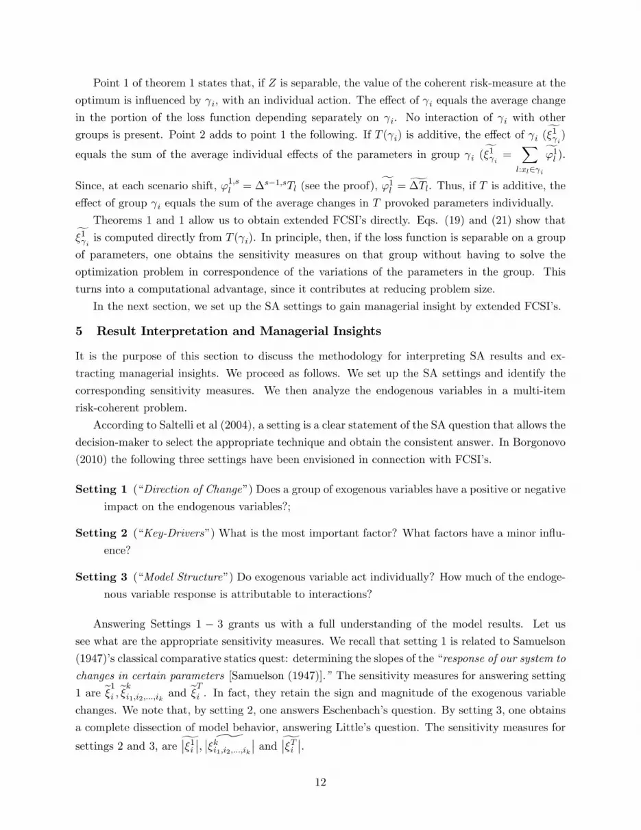
Point 1 of theorem 1 states that, if Z is separable, the value of the coherent risk-measure at the

optimum is in�uenced by i, with an individual action. The e¤ect of i equals the average change

in the portion of the loss function depending separately on i. No interaction of i with other

groups is present. Point 2 adds to point 1 the following. If T ( i) is additive, the e¤ect of i (f�1 i)

equals the sum of the average individual e¤ects of the parameters in group i (f�1 i = X

l:xl2 i

f'1l ).Since, at each scenario shift, '1;sl = �s�1;sTl (see the proof), f'1l = g�Tl. Thus, if T is additive, thee¤ect of group i equals the sum of the average changes in T provoked parameters individually.

Theorems 1 and 1 allow us to obtain extended FCSI�s directly. Eqs. (19) and (21) show thatf�1 i is computed directly from T ( i). In principle, then, if the loss function is separable on a group

of parameters, one obtains the sensitivity measures on that group without having to solve the

optimization problem in correspondence of the variations of the parameters in the group. This

turns into a computational advantage, since it contributes at reducing problem size.

In the next section, we set up the SA settings to gain managerial insight by extended FCSI�s.

5 Result Interpretation and Managerial Insights

It is the purpose of this section to discuss the methodology for interpreting SA results and ex-

tracting managerial insights. We proceed as follows. We set up the SA settings and identify the

corresponding sensitivity measures. We then analyze the endogenous variables in a multi-item

risk-coherent problem.

According to Saltelli et al (2004), a setting is a clear statement of the SA question that allows the

decision-maker to select the appropriate technique and obtain the consistent answer. In Borgonovo

(2010) the following three settings have been envisioned in connection with FCSI�s.

Setting 1 (�Direction of Change�) Does a group of exogenous variables have a positive or negativeimpact on the endogenous variables?;

Setting 2 (�Key-Drivers�) What is the most important factor? What factors have a minor in�u-ence?

Setting 3 (�Model Structure�) Do exogenous variable act individually? How much of the endoge-nous variable response is attributable to interactions?

Answering Settings 1 � 3 grants us with a full understanding of the model results. Let ussee what are the appropriate sensitivity measures. We recall that setting 1 is related to Samuelson

(1947)�s classical comparative statics quest: determining the slopes of the �response of our system to

changes in certain parameters [Samuelson (1947)].�The sensitivity measures for answering setting

1 are e�1i ;e�ki1;i2;:::;ik and e�Ti . In fact, they retain the sign and magnitude of the exogenous variablechanges. We note that, by setting 2, one answers Eschenbach�s question. By setting 3, one obtains

a complete dissection of model behavior, answering Little�s question. The sensitivity measures for

settings 2 and 3, are g���1i ��; ^���ki1;i2;:::;ik �� and g���Ti ��.12

We now address the selection of the endogenous variables. In a post-optimality analysis, a

decision-maker is interested in the optimal policy and in the value of the objective function at the

optimum [Monahan (2000)]. In a risk-coherent problem, these values are y� and ��. In a multi-item

problem y� is a vector of size n. Information consists of a 2n � I sensitivity matrix containing theextended FCSI�s of each xi, i = 1; 2; ::; n on each yr, r = 1; 2; :::; I. As the problem size increases,

result communication might become less straightforward.

A �rst way to reduce problem size is to consider, instead of the itemized list, the total number of

ordered items, i.e., ky�k. ky�k provides synthetic information on optimal order policies and has beenadopted in Borgonovo and Peccati (2009a). However, by synthesizing y� into its norm, one looses

information on the detailed e¤ect of exogenous variables. A second approach is to retain the vector

y� and integrate the analysis by Savage score correlation coe¢ cients (SSCCs). SSCCs have been

introduced by Iman and Conover (1987) to let decision-makers know whether exogenous variables

in�uence di¤erent endogenous variables in the same way. In the context of multi-item inventories,

we build them as follows. Denote by Rri the ranking of exogenous variable xi, when the optimal

order quantity of item r (y�r ) is the endogenous variable (the complete ranking of the parameters

is Rr = [Rr1; Rr2; :::; R

rn]). The corresponding vector of Savage scores is SS

r = [SSr1 ; SSr2 ; :::; SS

rn],

where

SSri =nX

j=Rri

1

j(24)

Similarly, let Rsi be the ranking of xi when item s is considered (Rs = [Rs1; Rs2; :::; R

sn]). Then, one

computes the correlation coe¢ cients �Rr;Rs and �SSr;SSs . A high value of �Rr;Rs denotes an overall

ranking agreement both when in�uential (top-ranked) and non-in�uential (low-ranked) parameters

are considered. �SSr;SSs informs us of whether the ranking agreement is at the top-ranked factors.

Comparing �SSr;SSr against �Rr;Rs one obtains information on whether the key-drivers of the

problem are the same [Iman and Conover (1987), Campolongo and Saltelli (1997), Kleijnen and

Helton (1999)].

We are then equipped with the tools necessary to examine the sensitivity of y�, jjy�jj and ��

as endogenous variables of a risk-coherent problem. In the next section, we present results and

managerial insights.

6 A Numerical Case Study

In this section, we illustrate the methodology developed in Sections 2, 3 and 5 by applying it to

a risk-coherent case study. The case study is based on the risk neutral (Rockafellar and Uryasev

(2002)) and conditional value at risk (CVaR) problems developed in Borgonovo and Peccati (2009a).

Let I denote the number of inventoried items. ! = [!1; !2; :::; !I ], ! 2�R+ the random demand

for items in the inventory, and (;; F ) the corresponding measure space. The exogenous variables

are revenues per unit of inventoried goods (r = [r1; r2; :::; rI ]), �xed order costs (a = [a1; a2; :::; aI ])

and holding costs per unit of inventoried item (c = [c1; c2; :::; cI ]). Hence, x = fa; c; rg. The system

13

loss function is:

Z(y;;x) = 1a+

IXi=1

!iciy2i

2� ry (25)

Note that the loss function in eq. (25) is additively separable in �xed costs. The corresponding

risk-neutral and risk-coherent problems are

Prisk�neutral =(miny�0

1a+

IXi=1

miciy2i

2� ry (26)

where mi := EFh1!i

i, and

PCV aR� =(

miny;�2S�R

� +1

1� �

"(1a� ry � �)F �+! +

IXi=1

ciy2im

�+i

2

#)(27)

where �+ = f! : Z > �+g, m�+i :=

R�+

1

!iand F �+! =

R�+dF (See Borgonovo and Peccati

(2009a) for further details.) The endogenous variables of interest are y�risk�neutral, jjy�risk�neutraljj,E[Z�] for Prisk�neutral, and y�CV aR, jjy�CV aRjj and CV aR� for PCV aR� .

Theorems 3 and 1 allow us to state the following results concerning the sensitivity of the en-

dogenous variables on �xed costs, before running both the optimization and sensitivity algorithms.

Proposition 1 1. e�1a = e�1a;r = e�1a;c = e�1a;c;r = 0 for y�risk�neutral, jjy�risk�neutraljj,y�CV aR,jjy�CV aRjj;

2. For both CV aR�� and E[Z�], then

e�1a;r = e�1a;c = e�1a;c;r = 0and

e�1a = IXi=1

g�ai = e�Ta (28)

where g�ai =Pps=1

asi � as�1i

pis the average of the changes in the �xed cost of item i.

Proof. The system loss function is additively separable in a.

1. Point 1 follows by Theorem 1.

2. Point 2 follows by Theorem 1. In fact, item 2 in Theorem 1 states that e�1a = IXl=1

�̂Tl(al).

By eq. (25), �s�1!sTl(al) = �s�1!sal, which, by averaging, leads to eq. (28). Also, by the

separability of eq. (25) and Point 1 in Theorem 1, all interactions e¤ects associated with a

are null. Hence, e�1a = IXi=1

g�ai = e�Ta .14

Table 2: Values of the exogenous variables in the central scenario.

Item 1 2 3 4 5 6 7 8 9 10r 10 11 12:5 13 12 9:5 14 13:5 12:5 15

a 1 2 2:5 1:5 1:8 2:2 2:3 4:1 1:9 2:7

c :55 :6 :65 :71 :53 :56 :68 :81 :92 :5

Table 3: Finite changes incurred by the endogenous variables as the exogenous variables varyacross the 6 scenarios

s! s+ 1 0! 1 1! 2 2! 3 3! 4 4! 5 5! 6

�s!s+1jjy�risk�neutraljj �40 �36 �32 �29 �27 �24�s!s+1E[Z�] �172 �181 �189 �195 �201 �207�s!s+1jjy�CV aRjj �18 �16 �14 �13 �12 �13�s!s+1CV aR�� �74 �78 �81 �84 �86 �88

Proposition 1 states that: i) for the system at hand, the risk-neutral and CVaR optimal policies

are insensitive on �xed costs; and ii) the �xed costs extended FCSI�s [eq. (28)] are exactly equal

to the sum of the average variations in �xed costs for both CV aR�� and E[Z�].We now examine whether numerical �ndings con�rm these expectations. As in Borgonovo and

Peccati (2009a), we consider a 10-item inventory (I = 10). The numerical values of r;a; c in the

base-case scenario are reported in Table 2.

The decision-maker assesses the following exogenous variable ranges: r 2 [:9r; 1:1r], a 2[0:85a; 1:15a] and c 2 [:8c; 1:2c], respectively. Each range is split into p = 7 subintervals. Seven

scenarios are then generated by the decision-maker, augmenting the parameters across the levels.

One obtains 6 �nite model-output changes [�s�1!sg, s = 1; 2; ::; p � 1; see eq. (12).] Table 3displays the numerical values of the changes in jjy�risk�neutraljj, E[Z�], jjy�CV aRjj and CV aR��.

The second line in Table 3 shows that jjy�risk�neutraljj monotonically decreases across scenario(�s�1!sjjy�risk�neutraljj < 0, s = 1; 2; :::; 6). The magnitude of the jumps decreases (

���s�1!sjjy�risk�neutraljj�� <�s!s+1jjy�risk�neutraljj, 8s). The behavior of jjy�CV aRjj is similar (Line 4). Line 3 shows that theexpected loss, E[Z�] monotonically decreases across the scenarios. The magnitude of the changes,however, increases. The behavior of CV aR�� is similar to the behavior of E[Z�].

Little�s question, then, emerges: what has caused the outputs to came out as they did? To

answer the question, we estimate the extended group FCSI�s of the exogenous variables, by de-

composing each of the �nite changes in the objective function across the scenarios. Including the

evaluation at x0, this is equivalent to exploring X at 43 points. Figure 2 displays the FCSI�s for

the �rst jump across scenarios 0� 1 of jjy�Risk�Neutraljj, (�0!1y�Risk�Neutral = �40 units).The values of the �rst order indices in Figure 2 are �1r = +72, �

1a = 0, �

1c = �108, respectively.

This indicates that the 3:3% increase in r produces an increase of 72 units in the order policy, which

15

Figure 2: �1r; �1a; �

1c; �

2r;a; �

2r;c; �

2c;a; �

3r;a;c for the change in jjy�risk�neutraljj (the total number of

ordered items in the risk-neutral optimal policy) from scenario x0 to scenario x1. Note that thesum of the sensitivity indices equals the �nite change: �0!1y�Risk�Neutral = �1r + �

1a + �

1c + �

2r;a +

�2r;c + �2c;a + �

3r;a;c

Table 4: Extended FCSI�s for the case study. The last three columns report the total order FCSI�s

Output e�1r e�1a e�1c e�2r;a e�2r;c e�2c;a e�3r;a;c e�Tr e�Ta e�Tcjjy�Risk�Neutraljj 64 0 �92 0 �3 0 0 61 0 �95

E[Z�] �795 1:1 564 0 39 0 0 �756 1:1 564� 39jjy�CV aRjj 28 0 �40 0 �1 0 0 27 0 39

CV aR�� �343 1:1 243 0 17 0 0 �343 + 17 1:1 243 + 17

is opposed by the decrease of 108 units provoked by the 3:3% change in c. a have no e¤ect, as

expected. Overall, individual indices explain a decrease of 36 units, namely 90% of the change. The

remaining 10% is not reducible to individual e¤ects, but due to interactions. Of these, all interaction

e¤ects involving a are null, in accordance with Proposition 1. The additional decrease is, therefore,

provoked by the residual interaction between unit revenues and costs: Indeed, �2r;c = �4 (Figure 2).In terms of Setting 3, Figure 2 shows that results for the optimal policy jjy�Risk�Neutraljj are drivenby individual e¤ects, with interaction e¤ects playing a minor role.

Figure 2 explains the endogenous variable change across scenarios 0 and 1. Examination of the

scenario-by-scenario results, shows that the behavior registered in shift across scenarios 0 and 1 is

replicated at all jumps. Table 4 displays the extended FCSI�s [eq. (13)].

The �rst line in Table 4 refers to jjy�Risk�Neutraljj. It shows that changes in jjy�Risk�Neutraljjare mainly driven by the individual e¤ects of r and c, with interactions playing a minor role. r

16

Table 5: Total order FCSI�s for the parameters across the 7 scenarios. One notes their monoton-ically decreasing magnitude

Scenario 0� 1 1� 2 2� 3 3� 4 4� 5 5� 6�T;sr 68 65 62 59 56 54

�T;sc �113 �104 �97 �91 �85 �80�T;sa 0 0 0 0 0 0

is associated with an average increase of 64 units, c with an average decrease of 92 units, and

their interaction e¤ect is e�2r;c = �3. Table 5 details the total order FCSI�s across the scenarios forjjy�Risk�Neutraljj.

Table 5 shows a monotonically decreasing magnitude of the sensitivity measures as s increases.

This means that the exogenous variables impact jjy�Risk�Neutraljj with decreasing intensity. Thisexplains the decreasing magnitude of the model output changes registered in Table 3.

The second line in Table 4 displays the extended FCSI�s for the risk-neutral expected loss, E[Z�].One notes that r has a negative e¤ect on the expected loss. This is in accordance with intuition,

since an increase in revenues decreases the expected loss. c on the other hand, has a positive e¤ect

on the loss. On E[Z�] a has a non-null, albeit small e¤ect (e�1a = 1:1). By Proposition 1, one expectsthis value to be equal to the sum of the average changes in �xed costs. A numeric check con�rms

this expectation.

The fourth line in Table 4 displays the numerical values of the sensitivity measure for jjy�CV aRjj:Results show that jjy�CV aRjj behaves in a similar way as jjy�Risk�Neutraljj. The e¤ect of r is anaverage increase in jjy�CV aRjj of 28 units. This is compensated by the e¤ect of c, that causes adecrease of 40 units in jjy�CV aRjj. The action of r; c is mainly individual, with a small and negativeinteraction e¤ect of �1. All e¤ects associated with a are null. The �fth line in Table 4 showsthe sensitivity measures for CV aR��. r has a negative e¤ect (its increase reduces the expected

conditional loss). c has a positive e¤ect (its increase augments CV aR��). There e¤ect of a is equal

to e�1a =PIi=1

g�ai = 1:1, in accordance with expectations (Proposition 1).Let us now interpret the results in the light of the SA settings. We start with settings 1 and 3.

The values of the sensitivity measures reveal that it is the individual e¤ects of r and c that drive

changes in order policy, with �xed costs playing no role and interaction e¤ects playing a minor role.

In this respect, one notes that interaction e¤ects amplify the action of c, while they oppose the

action of r. Thus, the total e¤ect of c is higher then its individual e¤ect; conversely, the total e¤ect

of r is smaller than its individual e¤ect. The resulting total order sensitivity indices, e�Tr ;e�Ta ,e�Tc ; arereported in the last three columns in Table 4. We recall that total order sensitivity indices measure

the overall e¤ect of an exogenous variable [Saltelli et al (2000), Saltelli and Tarantola (2002), Saltelli

et al (2008)].

As far as Setting 2 is concerned, key-drivers are identi�ed by the magnitudes of the total

order sensitivity indices [eq. (14)]. Figure 3 displays g���Tr ��, g���Ta �� and g���Tc �� for jjy�Risk�Neutraljj,E[Z�]; jjy�CV aRjj and CV aR�� are reported.

17

Figure 3: Key-drivers of PCV aR� and Prisk�neutral.

One notes that c is the main driver of the optimal order policies, both in Prisk�neutral andPCV aR� . It is closely followed by r. Fixed costs play no role. Conversely, r is the main driver ofthe change in E[Z�] and CV aR�� at the optimum. It is followed by c, with a playing a minor role.

We now come to the item-by-item SA results. Figure 4 displays the FCSI�s of all orders for all

the items of y�risk�neutral = [y�1;y

�2; :::;y

�10]:

Figure 4 shows that a has a null e¤ect on the optimal order policy of all items. For all items,

increases in price increase the unit orders (e�1r > 0 for all items); increases in holding costs impacty�i (i = 1; 2:; ; ; :10) in the opposite direction (e�1c < 0). e�2r;c is the only interaction e¤ects and isnegative for all items. Furthermore, e�1c > e�1r >> e�2r;c for all items, signalling that individual e¤ectsprevail over interaction e¤ects.

Thus, the item-by-item response maintains the structure of the response for jjy�risk�neutraljj.The key-drivers are c and r, with a being non-relevant.

In order to check whether the in�uence of c, r and a is uniform across items, we compute

the Savage score correlation coe¢ cients (see Section 5). We have �Rr;Rs = 1 and �SSr;SSs = 1,

r; s = 1; 2; :::; 10 (r 6= s): This result indicates a uniform e¤ect of the parameters on the item-by-

item optimal order quantity. In other words, c in�uences the ordered quantity �rst any item y�ithe most, r ranks second and a third, even if the order quantities of each item are di¤erent and

also the changes across the scenarios.

Let us now examine the SA results for y�CV CV ar, Figure 5 reports the FCSI�s of all orders for

all items.

Figure 5 shows that c and r are the drivers of the change, individual e¤ects play a major role

in respect of interaction e¤ects.

18

Figure 4: e�1r;e�1a;e�1c;e�2r;a;e�2r;c;e�2c;a;e�3r;a;c for the inventoried items of y�risk�neutral. The horizontalaxis displays the item number.

19

Figure 5: e�1r;e�1a;e�1c;e�2r;a;e�2r;c;e�2c;a;e�3r;a;c for the inventoried items of y�CV aR.

20

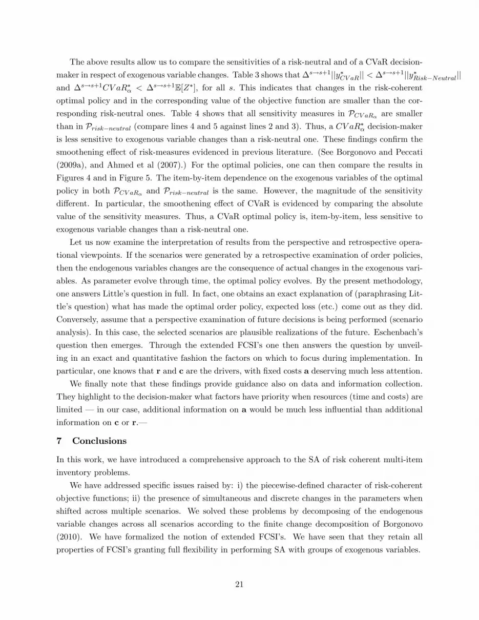
The above results allow us to compare the sensitivities of a risk-neutral and of a CVaR decision-

maker in respect of exogenous variable changes. Table 3 shows that�s!s+1jjy�CV aRjj < �s!s+1jjy�Risk�Neutraljjand �s!s+1CV aR�� < �s!s+1E[Z�], for all s: This indicates that changes in the risk-coherentoptimal policy and in the corresponding value of the objective function are smaller than the cor-

responding risk-neutral ones. Table 4 shows that all sensitivity measures in PCV aR� are smallerthan in Prisk�neutral (compare lines 4 and 5 against lines 2 and 3). Thus, a CV aR�� decision-makeris less sensitive to exogenous variable changes than a risk-neutral one. These �ndings con�rm the

smoothening e¤ect of risk-measures evidenced in previous literature. (See Borgonovo and Peccati

(2009a), and Ahmed et al (2007).) For the optimal policies, one can then compare the results in

Figures 4 and in Figure 5. The item-by-item dependence on the exogenous variables of the optimal

policy in both PCV aR� and Prisk�neutral is the same. However, the magnitude of the sensitivitydi¤erent. In particular, the smoothening e¤ect of CVaR is evidenced by comparing the absolute

value of the sensitivity measures. Thus, a CVaR optimal policy is, item-by-item, less sensitive to

exogenous variable changes than a risk-neutral one.

Let us now examine the interpretation of results from the perspective and retrospective opera-

tional viewpoints. If the scenarios were generated by a retrospective examination of order policies,

then the endogenous variables changes are the consequence of actual changes in the exogenous vari-

ables. As parameter evolve through time, the optimal policy evolves. By the present methodology,

one answers Little�s question in full. In fact, one obtains an exact explanation of (paraphrasing Lit-

tle�s question) what has made the optimal order policy, expected loss (etc.) come out as they did.

Conversely, assume that a perspective examination of future decisions is being performed (scenario

analysis). In this case, the selected scenarios are plausible realizations of the future. Eschenbach�s

question then emerges. Through the extended FCSI�s one then answers the question by unveil-

ing in an exact and quantitative fashion the factors on which to focus during implementation. In

particular, one knows that r and c are the drivers, with �xed costs a deserving much less attention.

We �nally note that these �ndings provide guidance also on data and information collection.

They highlight to the decision-maker what factors have priority when resources (time and costs) are

limited � in our case, additional information on a would be much less in�uential than additional

information on c or r.�

7 Conclusions

In this work, we have introduced a comprehensive approach to the SA of risk coherent multi-item

inventory problems.

We have addressed speci�c issues raised by: i) the piecewise-de�ned character of risk-coherent

objective functions; ii) the presence of simultaneous and discrete changes in the parameters when

shifted across multiple scenarios. We solved these problems by decomposing of the endogenous

variable changes across all scenarios according to the �nite change decomposition of Borgonovo

(2010). We have formalized the notion of extended FCSI�s. We have seen that they retain all

properties of FCSI�s granting full �exibility in performing SA with groups of exogenous variables.

21

We have obtained new results for the sensitivity analysis of risk-coherent optimization problems.

We have seen that, if a loss function (not necessarily describing an inventory system) is separable

in a group of exogenous variables, then the optimal policy is insensitive to that group. The risk-

measure-at-the-optimum is sensitive, with an additive response. These results hold for any change

and at all scenario jumps.

We have discussed the interpretation of results in the light three SA settings. We have seen

that one is endowed with the exact explanation of what has made the outputs come out as they did

(Little�s question) and with information about the factors on which to focus managerial attention

during implementation (Eschenbach�s question).

To illustrate the methodology, we have applied it to an inventory management case study,

involving a risk-neutral and CVaR problems. Numerical results con�rm the theoretical �ndings.

The extended FCSI�s of �xed costs are null on the optimal policy, and equal toIXi=1

g�ai on bothE[Z�] and CV aR��, due to the separable structure of the loss function. The sensitivity measuresallow us to identify the key drivers of the changes and unveil the detailed structure of the model

response across scenarios � in the speci�c case, only the interaction between c and r is relevant.

� The values of the sensitivity measures reveal that a CVaR decision-maker is less sensitive to

exogenous variable changes than a risk neutral one.

Acknowledgement 1 A signi�cant thanking goes to the anonymous referees for the perceptive

and thorough comments that have greatly contributed in improving the previous version of the work.

We also thank Prof. William Ferrell Jr., discussant of the paper at the Fifteenth Working Seminar

on Production Economics, for precious insights and comments. A thank also to Prof. Nico P.

Dellaert for insightful comments during the discussion of this work. Financial support from the

ELEUSI research center of Bocconi University is gratefully acknowledged by the authors.

References

[Ahmed et al (2007)] Ahmed S., Cakmak U. and Shapiro A., 2007: "Coherent Risk Measures

in Inventory Problems," European Journal of Operational Research, 182 (1), pp. 226-238.

[Artzner et al (1999)] Artzner P., Delbaen F., Eber J.M., Heath D., 1999: "Coherent

measures of risk," Mathematical Finance, 9, pp. 203-228.

[Bogataj and Cibej (1994)] Bogataj L. and Cibej J. A., 1994: �Perturbations in living stock

and similar biological inventory systems,�International Journal of Production Economics, 35 (1-

3), pp. 233-239.

[Borgonovo (2008)] Borgonovo E., 2008: �Di¤erential Importance and Comparative Statics: An

Application to Inventory Management,�International Journal of Production Economics, 111 (1),

pp. 170-179.

22

[Borgonovo (2010)] Borgonovo E., 2010: �Sensitivity Analysis with Finite Changes: an Appli-

cation to Modifed-EOQ Models�, European Journal of Operational Research, , 200, pp. 127�138.

[Borgonovo and Peccati (2009a)] Borgonovo E. and Peccati L., 2009a: �Risk Aversion in In-

ventory Management: Risk Averse vs Risk Neutral Policies�, International Journal of Production

Economics, 118 (1), pp. 233-242.

[Borgonovo and Peccati (2009b)] Borgonovo E. and Peccati L., 2009b: �Moment Calcula-

tions for Piecewise-De�ned Functions: An Application to Stochastic Optimization with Coherent

Risk Measures,�Annals of Operations Research, DOI: 10.1007/s10479-008-0504-1.

[Borgonovo and Peccati (2009c)] Borgonovo E. and Peccati L., 2009c: �Managerial Insights

from Service Industry Models: Generalizing Scenario Analysis�, Annals of Operational Research,

DOI 10.1007/s10479-009-0617-1.

[Campolongo and Saltelli (1997)] Campolongo F. and Saltelli A., 1997: �Sensitivity Analy-

sis of an Environmental Model: an Application of Di¤erent Analysis Methods,�Reliability Engi-

neering and System Safety, 57, pp. 49-69.

[Chen et al (2007)] Chen X., Sim M., Simchi-Levi D. and Sun P., 2007: " Risk Aversion in

Inventory Management," Operations Research, 55 (5), pp. 828�842.

[Eshenbach (1992)] Eschenbach T.G., 1992: �Spiderplots versus Tornado Diagrams for Sensi-

tivity Analysis,�Interfaces, 22, pp.40 -46.

[Gotoh and Takano (2007)] Gotoh J. and Takano Y., 2007: "Newsvendor Solutions via Con-

ditional Value-at-Risk Minimization," European Journal of Operational Research, 179 (1), pp.

80-96.

[Grubbström (2008)] Grubbstrõm R.W., 2008: "The Newsboy (Newsvendor) Problem when

Customer Demand is a Compound Renewal Process," Proceedings of the 15th Working Seminar

on Production Economics, Innsbruck, Austria, March 3-7 2008, pages 127-138.

[Higle and Wallace (2003)] Higle J.L. and Wallace S.W., 2003: �Sensitivity Analysis and

Uncertainty in Linear Programming,�Interfaces, 33 (4), pp. 53-60.

[Jansen et al (1997)] Jansen B., de Jong J.J., Roos C. and Terlaky T., 1997: �Sensitivity

Analysis in Linear Programming: Just be Careful!�, European Journal of Operational Research,

101, pp. 15-28.

[Jungermann and Thuring (1988)] Jungermann H. and Thuring M., 1988: �The Labyrinth of

Experts�Minds: Some Reasoning Strategies and Their Pitfalls�, Annals of Operations Research,

16, pp. 117-130.

23

[Kleijnen and Helton (1999)] Kleijnen, J.P.C. and J. Helton ,1999: �Statistical analyses of

scatter plots to identify important factors in large-scale simulations, 2: robustness of techniques,�

Reliability Engineering and Systems Safety, 65 (2), pp. 187-197.

[Koltay and Terlaki (2000)] Koltai T. and Terlaky T., 2000: �The di¤erence between the

managerial and mathematical interpretation of sensitivity analysis results in linear programming,�

International Journal of Production Economics, Volume 65, Issue 3 , 15 May 2000, pp. 257-274.

[Koltay and Tatay (2008)] Koltai T. and Tatay V., 2008: �A Practical Approach to Sensitivity

Analysis of Linear Programming under Degeneracy in Management Decision Making,�Proceedings

of the XV Working Seminar on Production Economics, Innsbruck, March 3-7, 2008, pp. 223-234.

[Iman and Conover (1987)] Iman R.L. and Conover W.J., 1987: �A Measure of Top-down

Correlation,�Technometrics, 29 (3), pp. 351-357.

[Little (1970)] Little J.D.C., 1970: �Models and Managers: The Concept of a Decision Calcu-

lus�, Management Science, 16 (8), Application Series, pp. B466-B485.

[Monahan (2000)] Monahan G.E., 2000: �Management Decision Making�, Cambridge Univer-

sity Press, Cambridge, U.K., 714 pages, ISBN-0521-78118-3.

[Myers and Montgomery (1995)] Myers R.H. and Montgomery D.C., 1995: �Response Sur-

face Methodology: Process and Product Optimization Using Designed Experiments,� John

Wyley&Sons, New York (USA), ISBN-978-0471581000.

[O�Brien (2004)] O�Brien F.A., 2004: �Scenario planning � lessons for practice from teaching

and learning�, European Journal of Operational Research, 152, pp. 709�722.

[Rabitz and Alis (1999)] Rabitz H. and Alis Ö. F., 1999: �General foundations of high-

dimensional model representations,�Journal of Mathematical Chemistry, 25, no. 2-3, pp. 197�233.

[Rockafellar and Uryasev (2002)] Rockafellar R.T. and S. Uryasev, 2002: "Conditional

Value-at-Risk for general loss distributions," Journal of Banking and Finance, 26, pp. 1443-1471.

[Ruszczynski and Shapiro (2005)] Ruszczy´nski A. and Shapiro A., 2005: "Optimization

of risk measures." in Probabilistic and Randomized Methods for Design under Uncertainty, G.

Cala�ore and F. Dabene (Eds.), Springer Verlag, London (UK).

[Saltelli et al (2000)] Saltelli A., Tarantola S. and Campolongo F., 2000: �Sensitivity

Analysis as an Ingredient of Modelling�, Statistical Science, 19 (4), pp. 377-395.

[Saltelli and Tarantola (2002)] Saltelli A. and Tarantola S., 2002: �On the Relative Impor-

tance of Input Factors in Mathematical Models: Safety Assessment for Nuclear Waste Disposal�,

Journal of the American Statistical Association, 97 (459), pp. 702-709.

24

[Saltelli et al (2004)] Saltelli A., Tarantola S., Campolongo F. and Ratto M., 2004:

�Sensitivity Analysis in Practice - a guide to assessing scienti�c models�, Wiley&Sons, Hoboken,

NJ, USA, 219 pages, ISBN 0-470-87093-1.

[Saltelli et al (2008)] Saltelli A., Ratto M., Andres T., Campolongo F., Cariboni J.,

Gatelli D., Saisana M. and Tarantola S., 2008: �Global Sensitivity Analysis: the Primer�,

Wiley&Sons, Chichester, West Sussex, England, 292 pages, ISBN 978-0-470-05997-5.

[Saltelli et al (2009)] Saltelli A, Cariboni J. and Campolongo F., 2009: �Screening im-

portant inputs in models with strong interaction properties,�Reliability Engineering and System

Safety, 94, pp. 1149�1155.

[Samuelson (1947)] Samuelson P., 1947: �Foundations of Economic Analysis,�Harvard Univer-

sity Press, Cambridge, MA.

[Tietje (2005)] Tietje 0., 2005: �Identi�cation of a small reliable and e¢ cientset of consistent

scenarios�, European Journal of Operational Research, 162, 418�432.

[Van Groenendaal and Kleijnen (2002)] Van Groenendaal W.J.H. and Kleijnen J.P.C.,

2002: "Deterministic versus stochastic sensitivity analysis in investment problems: An envi-

ronmental case study," European Journal of Operational Research, 141, pp. 8-20.

[Wallace (2000)] Wallace S.W., 2000: �Decision Making Under Uncertainty: is Sensitivity

Analysis of Any use?,�Operations Research, (1), pp. 20-25.

25