Tutorial: Consistent Representations of and

Conversions Between 3D Rotations

D. Rowenhorst 1, A.D. Rollett 2, G.S. Rohrer 2, M. Groeber 3,

M. Jackson 4, P.J. Konijnenberg 5, and M. De Graef 2 ‡1 The U.S. Naval Research Laboratory, 4555 Overlook Ave SW, Washington, DC

20375, USA

E-mail: David.Rowenhorst@nrl.navy.mil2 Department of Materials Science and Engineering, Carnegie Mellon University,

Pittsburgh, PA 15213, USA

E-mail: rollett@andrew.cmu.edu, rohrer@cmu.edu, degraef@cmu.edu3 Air Force Research Laboratory, Materials & Manufacturing Directorate, Wright

Patterson AFB, OH 45433, USA

E-mail: mike.groeber@gmail.com4 BlueQuartz Software, 400 S. Pioneer Blvd, Springboro, OH 45066, USA

E-mail: mike.jackson@bluequartz.net5 Max-Planck-Inst. fur Eisenforschung, Max-Planck-Str 1, 40237 Dusseldorf,

Germany

E-mail: p.konijnenberg@mpie.de

Abstract. In materials science the orientation of a crystal lattice is described by

means of a rotation relative to an external reference frame. A number of rotation

representations are in use, including Euler angles, rotation matrices, unit quaternions,

Rodrigues-Frank vectors and homochoric vectors. Each representation has distinct

advantages and disadvantages with respect to the ease of use for calculations and

data visualization. It is therefore convenient to be able to easily convert from

one representation to another. However, historically, each representation has been

implemented using a set of often tacit conventions; separate research groups would

implement different sets of conventions, thereby making the comparison of methods and

results difficult and confusing. This tutorial article aims to resolve these ambiguities

and provide a consistent set of conventions and conversions between common rotational

representations, complete with worked examples and a discussion of the trade-offs

necessary to resolve all ambiguities. Additionally, an open source Fortran-90 library of

conversion routines for the different representations is made available to the community.

Submitted to: Modelling Simulation Mater. Sci. Eng.

‡ Corresponding author: Department of Materials Science and Engineering, Carnegie Mellon

University, 5000 Forbes Avenue, Pittsburgh, PA 15213-3980, USA; Phone: (412) 268-8527, Fax: (412)

268-7596.

2

1. Introduction

While the laws of physics are usually expressed in a frame-invariant form, in practice, one

must nearly always select one or more reference frames with respect to which physical

quantities are expressed. In materials science and engineering, we use a variety of

reference frames to describe crystal structures and material properties (the Bravais

lattice); orientations of grains in microstructures (typically expressed in the sample

reference frame); grid coordinates in scanning-type data acquisitions (e.g., an acquisition

grid for electron back-scatter diffraction data sets); and so on. With the exception of

crystallographic reference frames, the majority of reference frames used in the materials

community are basic Cartesian frames, with orthonormal basis vectors.

The crystallographic reference frames have been defined for all crystal systems

by the International Union for Crystallography in the International Tables for

Crystallography (ITC), Volume A [1]. While the conventions of ITC are not always

strictly followed (e.g., crystal structures are often described in a non-standard space

group setting), on the whole the conventions of ITC-A are followed rather closely by most

researchers in the field. When crystallographic quantities are converted to a Cartesian

reference frame, however, there are several possible choices for the basis vectors (see

section 2.1 for more details), so that one must always be cautious when interpreting

crystallographic data that has been transformed to a Cartesian frame; for instance,

among the different commercial vendors of electron back-scatter diffraction (EBSD)

systems, different reference frame conventions are in use, making it sometimes difficult

to compare data for non-orthogonal crystal systems in particular. In this paper, we will

restrict our attention to the case of 3D rotations only, and assume that all reference

frames have the same origin.

The origin of this paper lies in a series of conversations between the co-authors

regarding the details of transformations between various rotation representations. It

became clear rather quickly that even in this small group of researchers, several

different conventions were being used, leading to different representations of the

same rotation and conflicting results. A small-scale “rotation round-robin” was

organized based on the following simple question: For the Euler angle triplet θ =

(ϕ1,Φ, ϕ2) = (2.721670, 0.148401, 0.148886) (radians) in the Bunge convention, what

are the equivalent numerical expressions for the axis-angle pair, quaternion, Rodrigues-

Frank vector, rotation matrix, and homochoric representations? All of these rotation

representations will be defined in detail later in this paper. The outcome of the round

robin was rather surprising: no two authors obtained exactly the same results, with

the most common difference being conflicting signs in those rotation representations

that involve the rotation axis explicitly. It should also be noted that only two of the

authors had implemented all six rotation representations; the others provided results

for a subset of the six representations. Given that all co-authors have many years of

experience in the field, it was quite surprising to find such a level of disagreement for

what was originally planned to be just an initial test to start a larger scale round robin.

3

While it is possible to perform nearly all texture-related computations using Euler

angles, recent years have seen an increased interest in the use of the so-called neo-

Eulerian representations of the form nf(ω), where n is a unit vector along the rotation

axis and ω the rotation angle. These representations, which will be defined in detail

in the next section, offer several advantages over Euler angles, but are perhaps not

as broadly understood in the materials community. With the recent availability of

open source software for 3-D materials science (e.g., the DREAM.3D package [2], or

the orilib library [3]), which implements many of these alternative representations, it

is becoming increasingly important for researchers to be aware of all sign conventions

when sharing source code. This tutorial paper is the direct result of a detailed analysis

of all orientation representations used in the materials community as well as all possible

sources for sign errors or ambiguities. The objective of this paper is to describe methods

that can be used to obtain accurate and consistent results when transforming from one

reference frame to another, independent of how the rotation is represented.

2. Definitions

In this section, we begin with the definition of the standard Cartesian reference frame.

Then we introduce the concept of a 3D rotation and define six different representations

or parameterizations commonly used in the materials field. Along the way, we have

several opportunities to make a selection between two options (for instance, left-handed

vs. right-handed, clockwise vs. counterclockwise, etc.); for each such selection, we will

explicitly state our choice as a convention. Some conventions will appear to be obvious,

but to avoid any uncertainty in later sections of this paper, we will explicitly state even

the obvious conventions.

2.1. Reference frames

The Bravais lattice is characterized by basis vectors ai (i = 1, . . . , 3), with unit cell edge

lengths (a, b, c) and angles (α, β, γ). The reciprocal lattice with basis vectors a∗j is then

defined by the relation

ai · a∗j = δij, (1)

where δij is the Kronecker delta; the reciprocal lattice parameters are (a∗, b∗, c∗) and

(α∗, β∗, γ∗). Using these two crystallographic lattices one then defines the standard

Cartesian (orthonormal) reference frame by the unit vectors ei. Although there are

infinite possibilities to do so, only a few orthonormalizations are frequently used:

These are all right-handed reference frames, i.e., e1 · (e2 × e3) = +1. Note that

this convention is not followed in all branches of science; for instance, in computer

graphics, left-handed Cartesian frames are quite common [5]. Hence, we formulate the

first convention:

Convention 1 When dealing with 3D rotations, all Cartesian reference frames will be

right-handed.

4

e1 a1/a a∗1/a∗ a∗1/a

∗

e2 e3 × e1 e3 × e1 a2/b

e3 a∗3/c∗ a3/c e1 × e2

Table 1. Frequently used orthonormalizations [4]. The first column is the preferred

choice listed in the International Tables for Crystallography [1].

2.2. 3D rotations

The turning of an object or a reference frame by a given angle ω about a fixed point d is

referred to as a rotation. Such an operation preserves the distances between the object

points as well as the handedness of the object. Each rotation has an invariant line,

represented by the unit vector n, which is known as the rotation axis; if the rotation is

represented by the operator R, then the action R(n) produces n again.

Consider a rotation characterized by d, n, and ω. The rotation angle ω is taken

to be positive for a counterclockwise rotation when looking from the end point of n

towards the fixed point d. For simplicity, and without loss of generality, we will from

here on take the fixed point to coincide with the origin of the reference frame, i.e. d = 0.

Convention 2 A rotation angle ω is taken to be positive for a counterclockwise rotation

when viewing from the end point of the rotation axis unit vector n towards the origin.

2.3. Rotation matrices and active and passive interpretations

A rotation can be viewed as operating on the object, which is the active interpretation,

or operating on the reference frame, which is the passive interpretation. An active

rotation transforms object coordinates to new coordinates in the same reference frame;

for the passive interpretation, the initial and final reference frames are different.

If we represent the rotated reference frame by the Cartesian basis vectors e′i,

then the components of these vectors with respect to the original basis ej form a

transformation matrix αij, defined in terms of the nine dot products:

αij = e′i · ej. (2)

The matrix αij defines a passive rotation from the old to the new reference frame, i.e.,

e′i = αijej, where we have used the Einstein summation convention for repeated indices.

For a vector p with components pj with respect to the basis vectors ej and p′i with

respect to e′i, we have the transformation rule:

p′i = αijpj. (3)

Rotation matrices belong to the set of special orthonormal matrices, SO(3), and have

the following properties: the determinant of the matrix is equal to +1; the transpose

of the matrix is equal to its inverse; and the sum of the squares of the entries in each

column/row equals +1.

5

It is common practice in the materials field, and particularly in the texture

community, to always consider 3D rotations as operating on reference frames, i.e., the

passive interpretation. We will follow this practice and formulate the third convention

as:

Convention 3 Rotations will be interpreted in the passive sense.

Therefore, for a crystal who’s standard Cartesian reference frame is rotated with

respect to the specimen reference frame, the orientation of the crystal will be described

as a passive rotation of the sample reference frame to coincide with the crystals standard

reference frame; in other words, the reference frame ei is the specimen reference frame,

and e′i represents the grain’s reference frame. The choice of the passive rotation

interpretation is a sensible choice, since the grains in a polycrystalline material do not

actually rotate; they have a stationary orientation with respect to the specimen reference

frame (except, perhaps, during deformation). In other fields of science and engineering,

the active rotation interpretation is the more natural one, for instance in the description

of the orientation of the segments of a robotic arm; in this case, the segments actually

do rotate themselves, so that the active interpretation is more suitable.

2.4. Euler angles

Euler has shown that any arbitrary 3D rotation can be decomposed into three successive

rotations around the coordinate axes. Since there are three independent axes, denoted

xyz for simplicity, there are several possibilities for the decomposition. The name Euler

angles is reserved for those decompositions for which two of the three axis symbols are

equal, as in zxz or yzy. Hence, there are six possible Euler angle conventions. When

the three axes are different, one refers to the angle triplet as Tayt-Briant angles ; while

they are used infrequently in materials science, they find frequent application in other

fields, for instance in aviation (roll, pitch, and yaw motions of an airplane).

In texture analysis, the most commonly used definition of the Euler angles is the

Bunge convention [6], which has an axis triplet zxz, with corresponding rotation angles

(ϕ1,Φ, ϕ2) (applied from left to right).

Convention 4 Euler angle triplets θ = (ϕ1,Φ, ϕ2) are implemented using the Bunge

convention, with the angular ranges as ϕ1 ∈ [0, 2π], Φ ∈ [0, π], and ϕ2 ∈ [0, 2π].

Note that, according to convention 3, the Euler angles are interpreted to represent

a rotated reference frame. To obtain the active interpretation, one must apply the

rotations with opposite angles, in the opposite order, (−ϕ2,−Φ,−ϕ1). The range

of the Euler angle triplet defined above results in a total volume in Euler space of

8π2 =∫∫∫

sin Φ dϕ1 dΦ dϕ2.

6

2.5. Axis-Angle pair

The axis angle pair representation, (n, ω) provides a convenient way of writing down a

rotation in terms of the angle ω and the axis n, which is typically represented either by

a crystallographic direction [uvw] or by a set of direction cosines [c1c2c3]. Note that for

non-cubic crystal systems, the normalization must be carried out on direction indices

that first have been transformed to the Cartesian reference frame. Often, the axis angle

pair is written in the form ω@n.

Convention 5 The rotation angle ω is limited to the interval [0, π].

For angles in the range ]π, 2π[, the sign of the unit axis vector n must be reversed,

and ω replaced by 2π − ω. For angles outside the range [0, 2π[, the angle must first be

reduced to the interval [0, 2π[ by adding or subtracting the appropriate integer multiple

of 2π. The main reason for limiting ω to the interval [0, π] is to allow for a seamless

conversion to the Rodrigues-Frank vector introduced in section 2.7.1.

2.6. Quaternions

A quaternion, q, is defined as a four-component number of the form q = q0+iq1+jq2+kq3,

where the imaginary units (i, j, k) satisfy the following relations:

i2 = j2 = k2 = −1; ij = −ji = k;

jk = −kj = i; ki = −ik = j. (4)

The quaternion is often written as q = (q0,q) with q0 the scalar part and q the vector

part; in component notation we have q = (q0, q1, q2, q3) or q = (q0, qi) with i = 1 . . . 3.

The definition (4) of the pairwise (ordered) products of the imaginary units leads to the

following expression for the quaternion product:

pq = (p0q0 − p · q, q0p + p0q + p× q);

= (p0q0 − prqr, q0pi + p0qi + εijkpjqk), (5)

where εijk is the permutation symbol, equal to +1 for even and −1 for odd permutations.

As usual, a summation is implied over repeated subscripts. The presence of a vector

cross-product in the vector part of the quaternion product implies that quaternion

multiplication does not commute, i.e., pq 6= qp.

The norm of a quaternion is defined as:

|q| = [q20 + q21 + q22 + q23]12 . (6)

Quaternions with unit norm are known as unit quaternions or versors, and they have

a special relationship with 3D rotations, similar to the relation between regular unit

complex numbers and 2D rotations. Unit quaternions can always be written in the form

q = cosω

2+ sin

ω

2(c1i + c2j + c3k) , (7)

7

where ci are the direction cosines of the rotation axis unit vector n. As a consequence of

convention 5, the scalar part q0 = cos(ω/2) of a unit quaternion representing a rotation

will always be positive (or 0 for rotations with rotation angle π).

Unit quaternions are located on the sphere S3 inside the 4D quaternion space. The

3D surface area of this sphere is equal to 2π2. One can show that the unit quaternions q

and −q represent the same rotation, so that all rotations can be represented by selecting

the entire Northern (q0 ≥ 0) hemisphere, which has surface area π2. Pure quaternions

have a zero scalar part and they will turn out to be useful to carry out rotations of

vectors. Despite the more complicated definition for quaternion multiplication, the

quaternion representation of rotations is numerically very convenient and widely used.

It is well known that a regular vector, r, can be rotated by means of quaternion

multiplications, provided we convert the vector to a quaternion/versor. We define the

quaternion rotation operator Lp( ), with p a unit quaternion, as follows:

Lp(r) ≡ vec [p(0, r)p∗] , (8)

where p∗ is the conjugate quaternion [p0,−p], and vec[ ] stands for the vector part of

the argument. In vector notation we obtain:

Lp(r) =(p20 − ||p||2

)r + 2(p · r)p + 2p0(p× r). (9)

The operator Lp(r) rotates the vector from one orientation to another orientation and is

hence an active operator. A simple example illustrates the use of the quaternion rotation

operator. Consider a rotation of 120◦@[111]; the corresponding unit quaternion is given

by:

p = (cosπ

3,

1√3

[111] sinπ

3) = (

1

2,1

2,1

2,1

2).

Taking r = [100] and using the vector expression (9) for the operator Lp( ), we obtain

Lp([100]) = [010],

as expected for an active rotation. If the conjugate of p is used, then we obtain:

Lp∗([100]) = [001],

so that passive rotations can be obtained simply by conjugating the quaternion p. This

is equivalent to transposing a rotation matrix to switch between active and passive

rotations.

The sign choices in equation (4) have become standard in the mathematical

literature and wherever quaternions are used in applications. It is therefore rather

interesting that in 1844, Sir Hamilton himself [7] discussed the possibility of a different

sign convention for the definition of quaternion multiplication. In section 5 of his 18-

installment paper published between 1844 and 1850, Hamilton writes that an entirely

consistent alternative definition of the quaternion product can be obtained by changing

the order in which the imaginary units are considered from the traditional (i, j, k) to

(k, j, i), so that the defining products become:

i2 = j2 = k2 = −1; ji = −ij = k; kj = −jk = i; ik = −ki = j. (10)

8

Note the sign reversals with respect to the standard definition. As a consequence of this

alternate definition, the quaternion product becomes:

pq = (p0q0 − p · q, q0p + p0q− p× q);

= (p0q0 − prqr, q0pi + p0qi − εijkpjqk), (11)

It is not too difficult to see that the standard definition of the quaternion product,

equation (5), corresponds to a right-handed triad (i, j, k) of imaginary units, whereas

the alternate definition in equation (11) corresponds to a left-handed triad (k, j, i). While

the right-handed quaternion product has become the standard in modern mathematics,

there is no reason not to consider the left-handed product as being on an equal footing.

One should note, and this will become important in the following section, that one could

also redefine the permutation symbol, εijk, to be −1 for even permutations and +1 for

odd permutations; in that case, one could maintain the plus sign in front of the vector

cross-product in equation 5 and the sign change caused by the left-handed imaginary

triad (k, j, i) would be hidden in the permutation symbol. In the remainder of this paper,

we prefer to keep the standard definition of the permutation symbol, and we will change

the definition of quaternion multiplication as needed by the application, as discussed in

Section 4.

2.7. Neo-Eulerian representations

The term neo-Eulerian was coined by Frank [8] and refers to rotation representations

of the form nf(ω), where f is a suitably chosen monotonic function of the rotation

angle. While there are many possible choices for this function, we will only introduce

two particular choices: the Rodrigues-Frank vector, and the homochoric vector.

2.7.1. Rodrigues-Frank vector The Rodrigues-Frank vector, ρ, is obtained by setting

f(ω) = tan(ω/2):

ρ = n tanω

2. (12)

Since the rotation angle belongs to the interval [0, π], all rotations around an axis n are

represented by points along the half-line formed by this unit vector, with a rotation by

π represented by the point at infinity (+∞). Rotation angles in the range [π, 2π] are

equivalent to setting the unit vector equal to its opposite, −n, and using a positive angle

2π − ω. Restricting the rotation angle to [0, π] (convention 5) has the added advantage

that tan(ω/2) is always positive and is thus equal to the length of the Rodrigues-Frank

vector ρ. Angles outside this range may cause a negative value for the tangent, which

would conflict with the positive nature of vector norms.

Given a Rodrigues-Frank vector ρ, the corresponding rotation angle can be derived

from ω = 2 arctan(|ρ|), which always results in an angle in the range [0, π], in agreement

with convention 5. Note that in source code, a Rodrigues-Frank vector should be stored

as a four-component vector, first the unit axis vector n, then the vector length tan(ω/2)

in the fourth position. This is necessary, so that a 180◦ rotation around an arbitrary

9

axis can be correctly represented without causing numerical overflows. The ANSI/IEEE

Standard 754-1985 (Standard for Binary Floating Point Arithmetic) defines how the

number +∞ is represented digitally; proper implementations of the Rodrigues-Frank

representation should adhere to this standard.

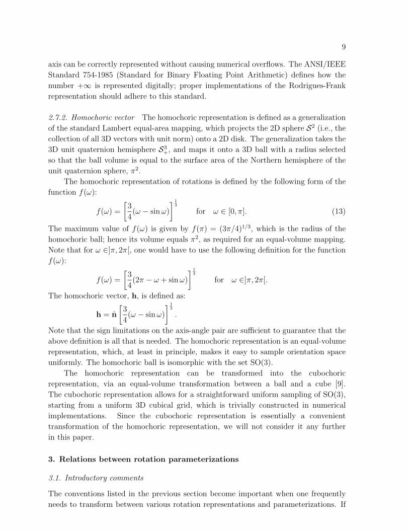
2.7.2. Homochoric vector The homochoric representation is defined as a generalization

of the standard Lambert equal-area mapping, which projects the 2D sphere S2 (i.e., the

collection of all 3D vectors with unit norm) onto a 2D disk. The generalization takes the

3D unit quaternion hemisphere S3+, and maps it onto a 3D ball with a radius selected

so that the ball volume is equal to the surface area of the Northern hemisphere of the

unit quaternion sphere, π2.

The homochoric representation of rotations is defined by the following form of the

function f(ω):

f(ω) =

[3

4(ω − sinω)

] 13

for ω ∈ [0, π]. (13)

The maximum value of f(ω) is given by f(π) = (3π/4)1/3, which is the radius of the

homochoric ball; hence its volume equals π2, as required for an equal-volume mapping.

Note that for ω ∈]π, 2π[, one would have to use the following definition for the function

f(ω):

f(ω) =

[3

4(2π − ω + sinω)

] 13

for ω ∈]π, 2π[.

The homochoric vector, h, is defined as:

h = n

[3

4(ω − sinω)

] 13

.

Note that the sign limitations on the axis-angle pair are sufficient to guarantee that the

above definition is all that is needed. The homochoric representation is an equal-volume

representation, which, at least in principle, makes it easy to sample orientation space

uniformly. The homochoric ball is isomorphic with the set SO(3).

The homochoric representation can be transformed into the cubochoric

representation, via an equal-volume transformation between a ball and a cube [9].

The cubochoric representation allows for a straightforward uniform sampling of SO(3),

starting from a uniform 3D cubical grid, which is trivially constructed in numerical

implementations. Since the cubochoric representation is essentially a convenient

transformation of the homochoric representation, we will not consider it any further

in this paper.

3. Relations between rotation parameterizations

3.1. Introductory comments

The conventions listed in the previous section become important when one frequently

needs to transform between various rotation representations and parameterizations. If

10

any one of the rotation representations is used by itself, then there is no need to apply

any of the conventions, as long as the selected representation is applied in an internally

consistent way. To consistently implement transformations between pairs of rotation

representations, however, requires the introduction of one additional convention.

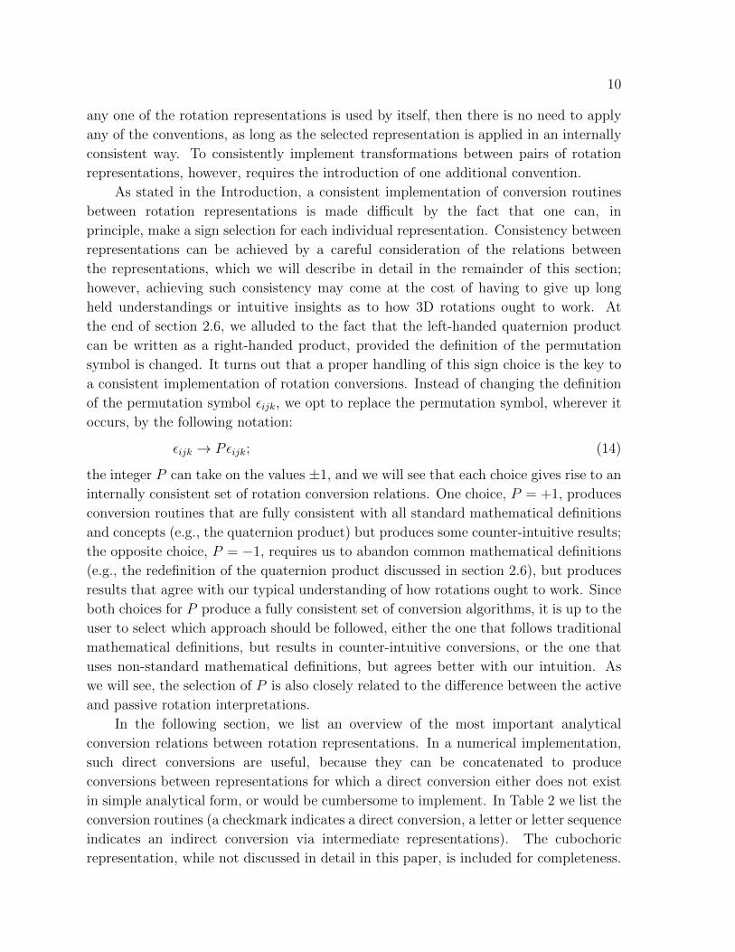
As stated in the Introduction, a consistent implementation of conversion routines

between rotation representations is made difficult by the fact that one can, in

principle, make a sign selection for each individual representation. Consistency between

representations can be achieved by a careful consideration of the relations between

the representations, which we will describe in detail in the remainder of this section;

however, achieving such consistency may come at the cost of having to give up long

held understandings or intuitive insights as to how 3D rotations ought to work. At

the end of section 2.6, we alluded to the fact that the left-handed quaternion product

can be written as a right-handed product, provided the definition of the permutation

symbol is changed. It turns out that a proper handling of this sign choice is the key to

a consistent implementation of rotation conversions. Instead of changing the definition

of the permutation symbol εijk, we opt to replace the permutation symbol, wherever it

occurs, by the following notation:

εijk → Pεijk; (14)

the integer P can take on the values ±1, and we will see that each choice gives rise to an

internally consistent set of rotation conversion relations. One choice, P = +1, produces

conversion routines that are fully consistent with all standard mathematical definitions

and concepts (e.g., the quaternion product) but produces some counter-intuitive results;

the opposite choice, P = −1, requires us to abandon common mathematical definitions

(e.g., the redefinition of the quaternion product discussed in section 2.6), but produces

results that agree with our typical understanding of how rotations ought to work. Since

both choices for P produce a fully consistent set of conversion algorithms, it is up to the

user to select which approach should be followed, either the one that follows traditional

mathematical definitions, but results in counter-intuitive conversions, or the one that

uses non-standard mathematical definitions, but agrees better with our intuition. As

we will see, the selection of P is also closely related to the difference between the active

and passive rotation interpretations.

In the following section, we list an overview of the most important analytical

conversion relations between rotation representations. In a numerical implementation,

such direct conversions are useful, because they can be concatenated to produce

conversions between representations for which a direct conversion either does not exist

in simple analytical form, or would be cumbersome to implement. In Table 2 we list the

conversion routines (a checkmark indicates a direct conversion, a letter or letter sequence

indicates an indirect conversion via intermediate representations). The cubochoric

representation, while not discussed in detail in this paper, is included for completeness.

11

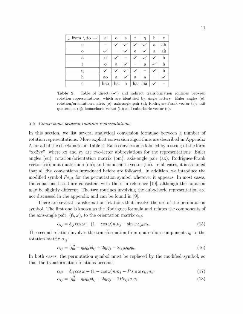
↓ from \ to → e o a r q h c

e – a ah

o – e a ah

a o – h

r o a – a h

q – h

h ao a a a –

c hao ha h ha ha –

Table 2. Table of direct ( ) and indirect transformation routines between

rotation representations, which are identified by single letters: Euler angles (e);

rotation/orientation matrix (o); axis-angle pair (a); Rodrigues-Frank vector (r); unit

quaternion (q); homochoric vector (h); and cubochoric vector (c).

3.2. Conversions between rotation representations

In this section, we list several analytical conversion formulae between a number of

rotation representations. More explicit conversion algorithms are described in Appendix

A for all of the checkmarks in Table 2. Each conversion is labeled by a string of the form

“xx2yy”, where xx and yy are two-letter abbreviations for the representations: Euler

angles (eu); rotation/orientation matrix (om); axis-angle pair (ax); Rodrigues-Frank

vector (ro); unit quaternion (qu); and homochoric vector (ho). In all cases, it is assumed

that all five conventions introduced before are followed. In addition, we introduce the

modified symbol Pεijk for the permutation symbol wherever it appears. In most cases,

the equations listed are consistent with those in reference [10], although the notation

may be slightly different. The two routines involving the cubochoric representation are

not discussed in the appendix and can be found in [9].

There are several transformation relations that involve the use of the permutation

symbol. The first one is known as the Rodrigues formula and relates the components of

the axis-angle pair, (n, ω), to the orientation matrix αij:

αij = δij cosω + (1− cosω)ninj − sinω εijknk. (15)

The second relation involves the transformation from quaternion components qi to the

rotation matrix αij:

αij = (q20 − qkqk)δij + 2qiqj − 2εijkq0qk. (16)

In both cases, the permutation symbol must be replaced by the modified symbol, so

that the transformation relations become:

αij = δij cosω + (1− cosω)ninj − P sinω εijknk; (17)

αij = (q20 − qkqk)δij + 2qiqj − 2Pεijkq0qk. (18)

12

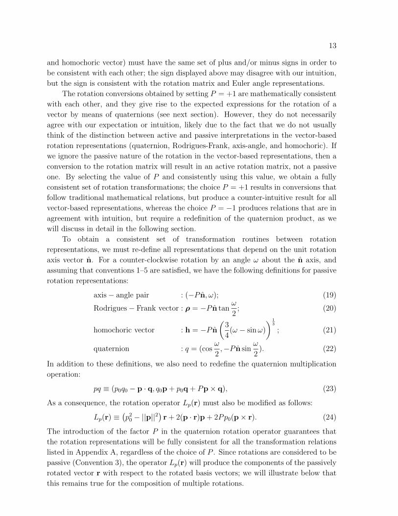
4. Discussion

4.1. Revisiting active vs. passive interpretations

The 19 conversion relations presented in Appendix A provide efficient numerical

pathways to switch from one rotation representation to another. They are fully

consistent with each other, regardless of the value of the constant P . The routines

have been implemented in an open source fortran-90 library, which is made available to

the community via the source code repository github.com [11].

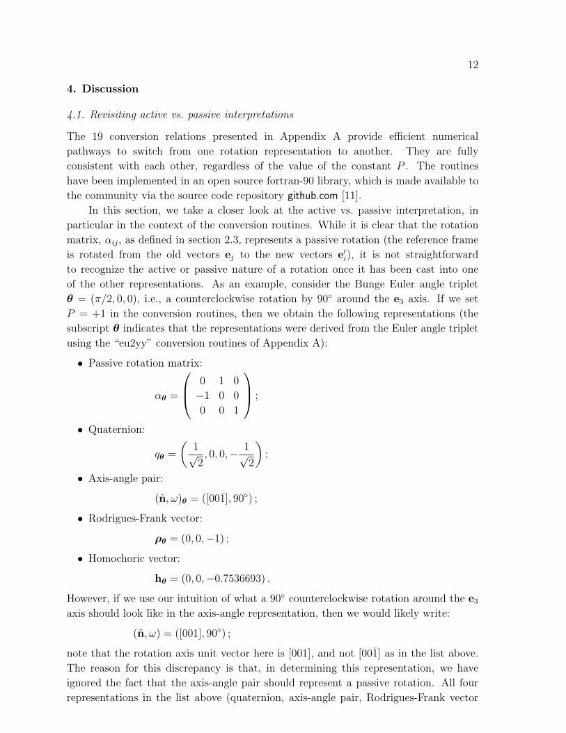
In this section, we take a closer look at the active vs. passive interpretation, in

particular in the context of the conversion routines. While it is clear that the rotation

matrix, αij, as defined in section 2.3, represents a passive rotation (the reference frame

is rotated from the old vectors ej to the new vectors e′i), it is not straightforward

to recognize the active or passive nature of a rotation once it has been cast into one

of the other representations. As an example, consider the Bunge Euler angle triplet

θ = (π/2, 0, 0), i.e., a counterclockwise rotation by 90◦ around the e3 axis. If we set

P = +1 in the conversion routines, then we obtain the following representations (the

subscript θ indicates that the representations were derived from the Euler angle triplet

using the “eu2yy” conversion routines of Appendix A):

• Passive rotation matrix:

αθ =

0 1 0

−1 0 0

0 0 1

;

• Quaternion:

qθ =

(1√2, 0, 0,− 1√

2

);

• Axis-angle pair:

(n, ω)θ = ([001], 90◦) ;

• Rodrigues-Frank vector:

ρθ = (0, 0,−1) ;

• Homochoric vector:

hθ = (0, 0,−0.7536693) .

However, if we use our intuition of what a 90◦ counterclockwise rotation around the e3

axis should look like in the axis-angle representation, then we would likely write:

(n, ω) = ([001], 90◦) ;

note that the rotation axis unit vector here is [001], and not [001] as in the list above.

The reason for this discrepancy is that, in determining this representation, we have

ignored the fact that the axis-angle pair should represent a passive rotation. All four

representations in the list above (quaternion, axis-angle pair, Rodrigues-Frank vector

13

and homochoric vector) must have the same set of plus and/or minus signs in order to

be consistent with each other; the sign displayed above may disagree with our intuition,

but the sign is consistent with the rotation matrix and Euler angle representations.

The rotation conversions obtained by setting P = +1 are mathematically consistent

with each other, and they give rise to the expected expressions for the rotation of a

vector by means of quaternions (see next section). However, they do not necessarily

agree with our expectation or intuition, likely due to the fact that we do not usually

think of the distinction between active and passive interpretations in the vector-based

rotation representations (quaternion, Rodrigues-Frank, axis-angle, and homochoric). If

we ignore the passive nature of the rotation in the vector-based representations, then a

conversion to the rotation matrix will result in an active rotation matrix, not a passive

one. By selecting the value of P and consistently using this value, we obtain a fully

consistent set of rotation transformations; the choice P = +1 results in conversions that

follow traditional mathematical relations, but produce a counter-intuitive result for all

vector-based representations, whereas the choice P = −1 produces relations that are in

agreement with intuition, but require a redefinition of the quaternion product, as we

will discuss in detail in the following section.

To obtain a consistent set of transformation routines between rotation

representations, we must re-define all representations that depend on the unit rotation

axis vector n. For a counter-clockwise rotation by an angle ω about the n axis, and

assuming that conventions 1–5 are satisfied, we have the following definitions for passive

rotation representations:

axis− angle pair : (−P n, ω); (19)

Rodrigues− Frank vector : ρ = −P n tanω

2; (20)

homochoric vector : h = −P n

(3

4(ω − sinω)

) 13

; (21)

quaternion : q = (cosω

2,−P n sin

ω

2). (22)

In addition to these definitions, we also need to redefine the quaternion multiplication

operation:

pq ≡ (p0q0 − p · q, q0p + p0q + Pp× q), (23)

As a consequence, the rotation operator Lp(r) must also be modified as follows:

Lp(r) ≡(p20 − ||p||2

)r + 2(p · r)p + 2Pp0(p× r). (24)

The introduction of the factor P in the quaternion rotation operator guarantees that

the rotation representations will be fully consistent for all the transformation relations

listed in Appendix A, regardless of the choice of P . Since rotations are considered to be

passive (Convention 3), the operator Lp(r) will produce the components of the passively

rotated vector r with respect to the rotated basis vectors; we will illustrate below that

this remains true for the composition of multiple rotations.

14

4.2. Vector transformations and quaternion-based consecutive rotations

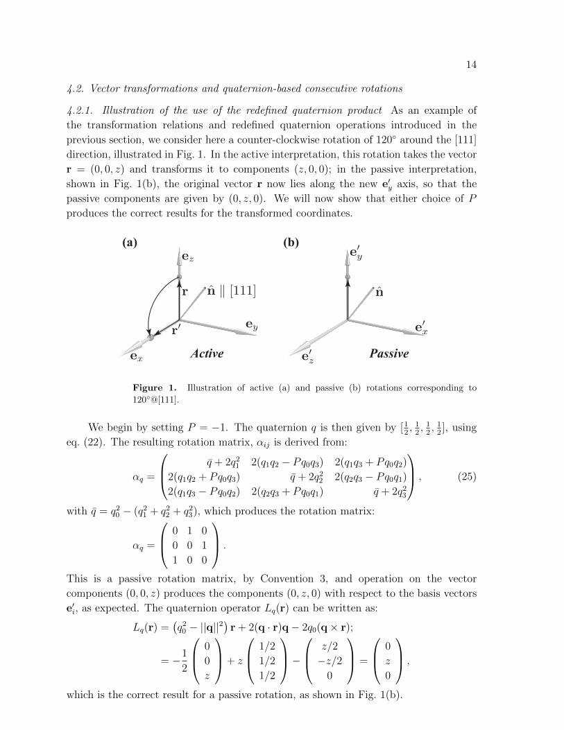
4.2.1. Illustration of the use of the redefined quaternion product As an example of

the transformation relations and redefined quaternion operations introduced in the

previous section, we consider here a counter-clockwise rotation of 120◦ around the [111]

direction, illustrated in Fig. 1. In the active interpretation, this rotation takes the vector

r = (0, 0, z) and transforms it to components (z, 0, 0); in the passive interpretation,

shown in Fig. 1(b), the original vector r now lies along the new e′y axis, so that the

passive components are given by (0, z, 0). We will now show that either choice of P

produces the correct results for the transformed coordinates.

(a) (b)

Active Passive

Figure 1. Illustration of active (a) and passive (b) rotations corresponding to

120◦@[111].

We begin by setting P = −1. The quaternion q is then given by [12, 12, 12, 12], using

eq. (22). The resulting rotation matrix, αij is derived from:

αq =

q + 2q21 2(q1q2 − Pq0q3) 2(q1q3 + Pq0q2)

2(q1q2 + Pq0q3) q + 2q22 2(q2q3 − Pq0q1)2(q1q3 − Pq0q2) 2(q2q3 + Pq0q1) q + 2q23

, (25)

with q = q20 − (q21 + q22 + q23), which produces the rotation matrix:

αq =

0 1 0

0 0 1

1 0 0

.

This is a passive rotation matrix, by Convention 3, and operation on the vector

components (0, 0, z) produces the components (0, z, 0) with respect to the basis vectors

e′i, as expected. The quaternion operator Lq(r) can be written as:

Lq(r) =(q20 − ||q||2

)r + 2(q · r)q− 2q0(q× r);

= −1

2

0

0

z

+ z

1/2

1/2

1/2

− z/2

−z/20

=

0

z

0

,

which is the correct result for a passive rotation, as shown in Fig. 1(b).

15

For the opposite sign choice, P = +1, the quaternion becomes q = [12,−1

2,−1

2,−1

2],

following eq. (22). The rotation matrix αq remains the same, due to the fact that the

factor P in eq. (25) compensates for the sign change. The quaternion rotation operator

now becomes:

Lq(r) =(q20 − ||q||2

)r + 2(q · r)q + 2q0(q× r);

= −1

2

0

0

z

+ z

1/2

1/2

1/2

+

−z/2z/2

0

=

0

z

0

,

which is once again the correct result. Note that the sign change of the last term with

respect to the P = −1 case illustrated before is compensated by the sign change in the

vector part of the quaternion.

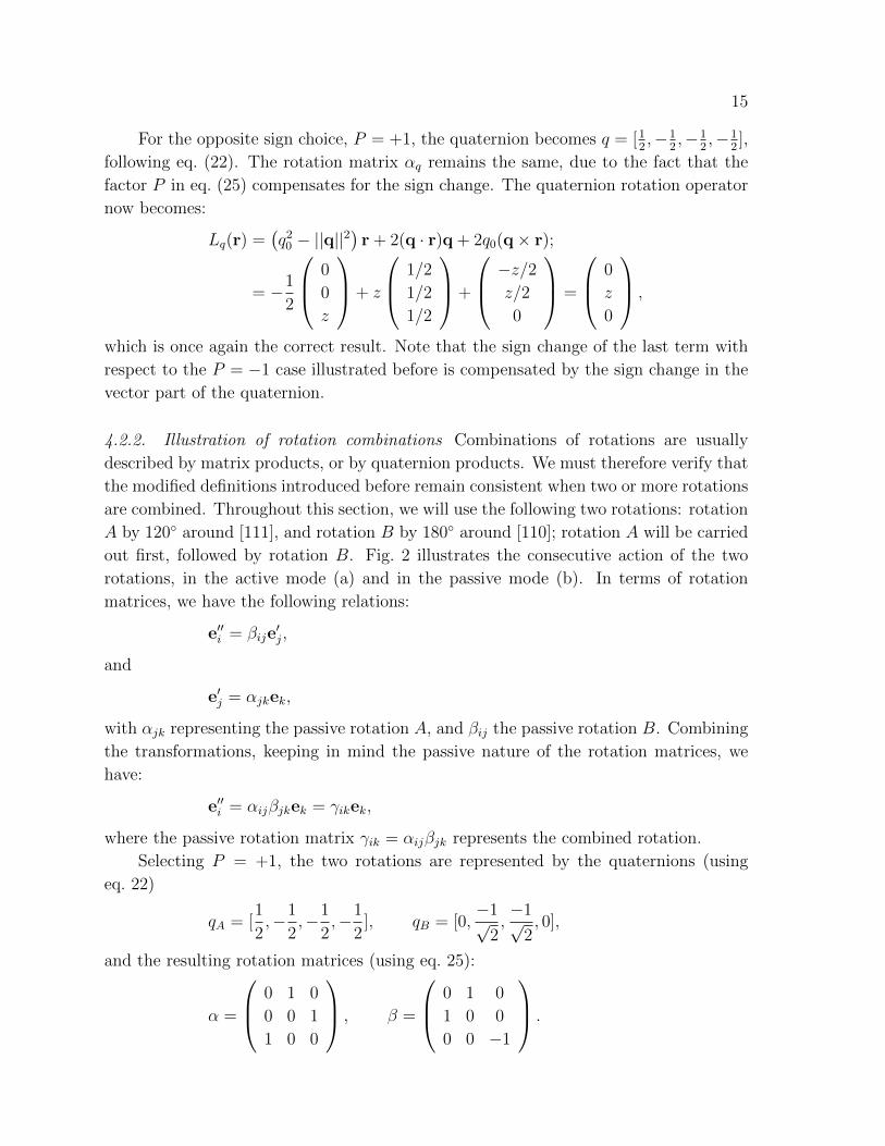
4.2.2. Illustration of rotation combinations Combinations of rotations are usually

described by matrix products, or by quaternion products. We must therefore verify that

the modified definitions introduced before remain consistent when two or more rotations

are combined. Throughout this section, we will use the following two rotations: rotation

A by 120◦ around [111], and rotation B by 180◦ around [110]; rotation A will be carried

out first, followed by rotation B. Fig. 2 illustrates the consecutive action of the two

rotations, in the active mode (a) and in the passive mode (b). In terms of rotation

matrices, we have the following relations:

e′′i = βije′j,

and

e′j = αjkek,

with αjk representing the passive rotation A, and βij the passive rotation B. Combining

the transformations, keeping in mind the passive nature of the rotation matrices, we

have:

e′′i = αijβjkek = γikek,

where the passive rotation matrix γik = αijβjk represents the combined rotation.

Selecting P = +1, the two rotations are represented by the quaternions (using

eq. 22)

qA = [1

2,−1

2,−1

2,−1

2], qB = [0,

−1√2,−1√

2, 0],

and the resulting rotation matrices (using eq. 25):

α =

0 1 0

0 0 1

1 0 0

, β =

0 1 0

1 0 0

0 0 −1

.

16

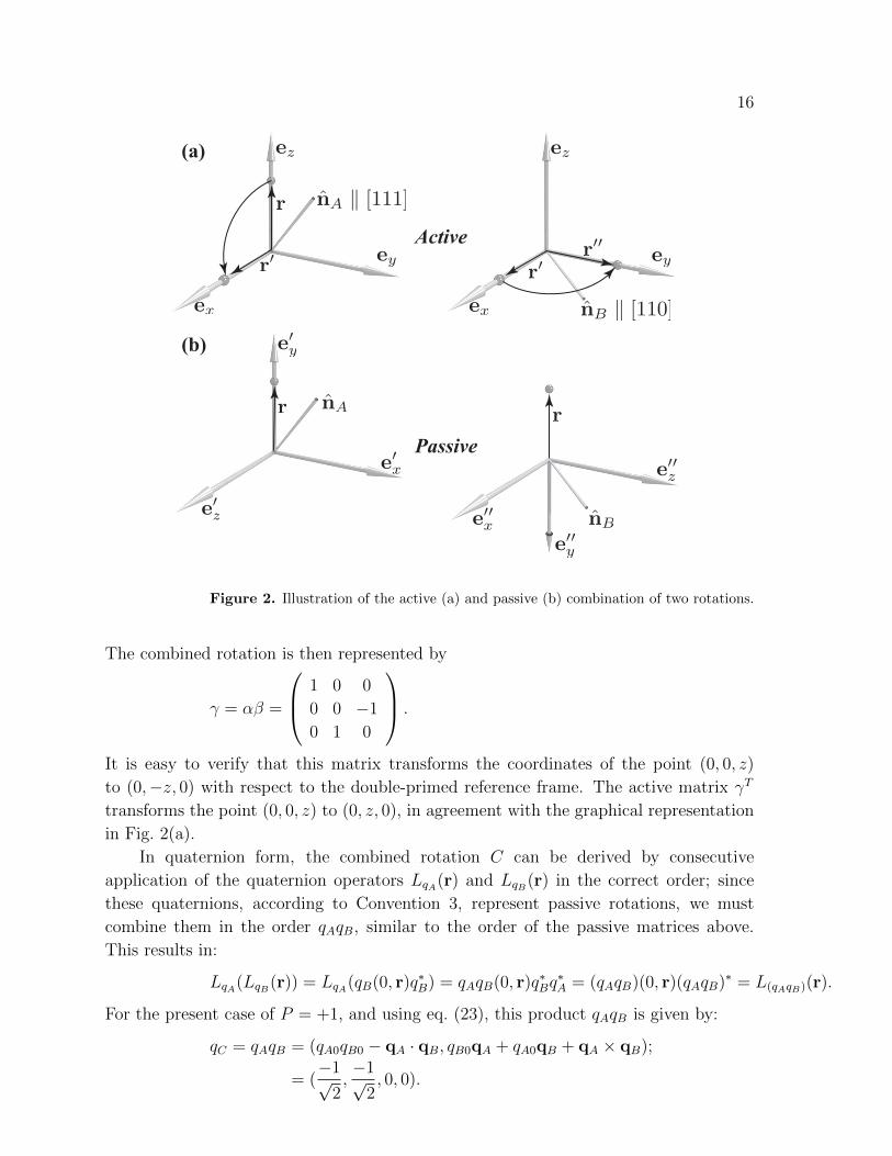
(a)

Active

Passive

(b)

Figure 2. Illustration of the active (a) and passive (b) combination of two rotations.

The combined rotation is then represented by

γ = αβ =

1 0 0

0 0 −1

0 1 0

.

It is easy to verify that this matrix transforms the coordinates of the point (0, 0, z)

to (0,−z, 0) with respect to the double-primed reference frame. The active matrix γT

transforms the point (0, 0, z) to (0, z, 0), in agreement with the graphical representation

in Fig. 2(a).

In quaternion form, the combined rotation C can be derived by consecutive

application of the quaternion operators LqA(r) and LqB(r) in the correct order; since

these quaternions, according to Convention 3, represent passive rotations, we must

combine them in the order qAqB, similar to the order of the passive matrices above.

This results in:

LqA(LqB(r)) = LqA(qB(0, r)q∗B) = qAqB(0, r)q∗Bq∗A = (qAqB)(0, r)(qAqB)∗ = L(qAqB)(r).

For the present case of P = +1, and using eq. (23), this product qAqB is given by:

qC = qAqB = (qA0qB0 − qA · qB, qB0qA + qA0qB + qA × qB);

= (−1√

2,−1√

2, 0, 0).

17

According to Convention 5, the scalar part of the quaternion must be positive, so

we change the sign of all the quaternion components. Using the quaternion rotation

operator LqC (r) (eq. 24) with r = (0, 0, z) we find:

LqC (r) =(q2C0 − ||qC ||2

)r + 2(qC · r)qC + 2qC0(qC × r) = (0,−z, 0) ,

in agreement with Fig. 2(b).

For the case P = −1, the quaternions are given by (using eq. 22):

qA = [1

2,1

2,1

2,1

2], qB = [0,

1√2,

1√2, 0],

and the resulting rotation matrices (using eq. 25) are identical to the matrices listed

before. Using eq. (23), we have for the quaternion product:

qC = qAqB = (1√2,−1√

2, 0, 0),

where Convention 5 has been applied. Using the quaternion operator LqC (r) (eq. 24)

with r = (0, 0, z) we find:

LqC (r) =(q2C0 − ||qC ||2

)r + 2(qC · r)qC − 2qC0(qC × r) = (0,−z, 0) ,

once again in agreement with Fig. 2(b). To achieve active rotations, the quaternion qCmust be conjugated before the operator LqC (r) is applied, i.e., Lq∗c (r).

The conclusion from this explicit example is that the revised definitions of

the quaternion operators found in section 4.1 provide a consistent framework for

transformations between rotations, as well as for the concatenation of multiple rotations.

Either sign choice for P leads to a fully internally consistent set of transformation and

composition rules, valid across all the rotation representations described in this paper.

5. Summary

In this tutorial paper, we have described a consistent approach to conversions

between different rotation representations and parameterizations commonly used in

the materials community. We have stated six conventions (mostly sign conventions)

that need to be followed to achieve an internally consistent set of transformation

routines; 19 explicit transformation routines between representations are described in

the appendix. This paper is the result of a small scale “rotation round-robin”, carried out

amongst the authors, which revealed several sign differences between individual author’s

implementations. The recent availability of open source software for 3-D materials

science (e.g., DREAM.3D), for which many researchers are contributing code, has made

it clear that there is a need for agreed-upon rotation conventions, so that, from the

start, source code generated by different research groups can be written in a way that

is readily compatible with the larger project code. When dealing with 3-D rotation

representations, there are too many opportunities for sign errors and confusion, and it

is hoped that the present paper will provide a guide to researchers in the field.

18

The main message of this tutorial paper is that there are two alternative ways of

implementing rotation transformation routines. The two approaches can be selected

by means of a simple parameter, P , which takes on the values ±1, and are readily

implemented in any modern programming language; a Fortran-90 version and an

Interactive Data Language (IDL, [12]) version are available from the authors, and

a C/C++ version is currently being implemented as part of the DREAM.3D open

source package. Effectively, the introduction of the parameter P as part of a

redefined permutation symbol, εijk → Pεijk, must be carried through in all rotation

transformation expressions, as well as in the definition of the quaternion product. All

neo-Eulerian rotation representations are also redefined in terms of the parameter P . It

is suggested that the selection of P be made at compilation time and that the selection

be described explicitly in the package documentation. An extensive test program that

exercises all the transformations through a series of general and special rotation cases

is also available from the authors; such a test program may prove to be valuable when

implementations in other programming languages are undertaken.

19

Acknowledgments

DJR would like to acknowledge the financial support of the Naval Research Laboratory

and the Structural Metallics Program of Office of Naval Research under contract #

N0001414WX20779. ADR acknowledges the support of the National Science Foundation

under contract # DMR 1435544. MDG would like to acknowledge the Air Force Office

of Scientific Research, MURI contract # FA9550-12-1-0458, for financial support.

20

References

[1] T. Hahn, editor. The International Tables for Crystallography Vol A: Space-Group Symmetry.,

volume A. Kluwer Academic Publishers, Dordrecht, 1989.

[2] M.A. Groeber and M.A. Jackson. DREAM.3D: A digital representation environment for the

analysis of microstructure in 3d. Integrating Materials and Manufacturing Innovation, 3:5,

2014.

[3] http://orilib.sourceforge.net/, 2015.

[4] C. Giacovazzo, H. L. Monaco, G. Artioli, D. Viterbo, G. Ferraris, G. Gilli, G. Zanotti, and M. Catti.

Fundamentals of Crystallography. Oxford University Press, Oxford GB, 2002.

[5] R. Salmon and M. Slater. Computer graphics: systems & concepts. Addison-Wesley (Wokingham,

England), 1987.

[6] H.-J. Bunge. Texture analysis in materials science: mathematical methods. Butterworths

(London), 1982.

[7] W.R. Hamilton. On quaternions; or on a new system of imaginaries in algebra. The London,

Edinburgh and Dublin Philosophical Magazine, xxv:10–13, 1844.

[8] F. Frank. Orientation mapping. Metall. Mater. Trans. A, 19:403–408, 1988.

[9] D. Rosca, A. Morawiec, and M. De Graef. A new method of constructing a grid in the space of

3D rotations and its applications to texture analysis. Modeling and Simulations in Materials

Science and Engineering, 22:075013, 2014.

[10] A. Morawiec. Orientations and Rotations: computations in crystallographic textures. Springer

Verlag, New York, 2004.

[11] http://www.github.com/marcdegraef/3drotations, 2015.

[12] http://www.exelisvis.com/productsservices/idl.aspx, 2015.

21

Appendix A. Conversions between rotation representations

In the following subsections, nineteen explicit rotation conversion algorithms are

described. For each conversion, the section title provides a shorthand indicator of the

conversion, with the first two letters describing the input representation, and the last two

characters the output representation; thus, eu2ro refers to the algorithm that converts an

Euler angle triplet into a Rodrigues-Frank vector, and ho2ax takes a homochoric vector

as input and converts it to an axis-angle pair. All algorithms below strictly adhere to the

sign conventions described in the main body of this paper. Upon implementing these

relations, the reader should exercise caution when using numerical implementations of

the arc-tangent function, for which both single argument and two-argument versions

exist in many programming languages; care must be taken to ensure that the resulting

angle satisfies convention 5.

Appendix A.1. eu2om

The Euler angle triplet θ = (ϕ1,Φ, ϕ2) can be converted into a rotation matrix by

multiplication of the individual (passive) rotation matrices:

α(θ) = αz′′(ϕ2)αx′(Φ)αz(ϕ1);

=

c1c2 − s1c s2 s1c2 + c1c s2 ss2−c1s2 − s1c c2 −s1s2 + c1c c2 sc2

s1 s −c1 s c

(A.1)

where ci = cosϕi, si = sinϕi, c = cos Φ, and s = sin Φ.

Appendix A.2. eu2ax

The axis-angle pair (n, ω) can be obtained from the Bunge Euler angles by using the

following relation:

(n, ω) =

(−Pτt cos δ,−P

τt sin δ,−P

τsinσ, α

)(A.2)

where

t = tanΦ

2; σ =

1

2(ϕ1 + ϕ2); δ =

1

2(ϕ1 − ϕ2);

τ =√t2 + sin2 σ; α = 2 arctan

τ

cosσ. (A.3)

If α > π, then the axis angle pair is given by:

(n, ω) =

(P

τt cos δ,

P

τt sin δ,

P

τsinσ, 2π − α

). (A.4)

Appendix A.3. eu2ro

This conversion involves first the conversion to the axis-angle pair, followed by

application of the definition of the Rodrigues-Frank vector in equation (12).

22

Appendix A.4. eu2qu

Starting from Euler angles in radians, we define

σ =1

2(ϕ1 + ϕ2); δ =

1

2(ϕ1 − ϕ2); c = cos

Φ

2; s = sin

Φ

2; (A.5)

The quaternion is then given by:

q = (c cosσ,−Ps cos δ,−Ps sin δ,−Pc sinσ) . (A.6)

If q0 becomes negative, then the sign of the entire quaternion has to be reversed,

q → −q, so that the resulting quaternion will lie in the Northern hemisphere of the

unit quaternion sphere.

Appendix A.5. om2eu

Let the rotation matrix be given by αij, then, if |α33| 6= 1, compute ζ as

ζ =1√

1− α233

. (A.7)

Then use the following relations to determine the angles:

θ = (atan2(α31ζ,−α32ζ), arccos(α33), atan2(α13ζ, α23ζ)) . (A.8)

where atan2 is the standard two argument implementation of the arc-tangent function,

i.e., atan2(y, x) produces the angle for which the tangent equals y/x. Note that the

order of the arguments needs to be reversed for some programming languages.

If |α33| = 1, i.e. Φ = 0 or π, then we can not determine a unique value for ϕ1

and ϕ2. We will use the convention that the entire angle is represented by ϕ1, and set

ϕ2 = 0, and we obtain:

θ =(

atan2(α12, α11),π

2(1− α33), 0

). (A.9)

Appendix A.6. om2ax

Starting from the rotation matrix αij, we compute the rotation angle via the trace of

the matrix:

ω = arccos

(1

2(Tr(α)− 1)

)If the rotation angle equals zero, the axis-angle pair becomes (n, ω) = ([001], 0). For

the direction cosines of the rotation axis, we determine the eigenvector of the rotation

matrix corresponding to the eigenvalue +1; it is well known that every rotation matrix

has three eigenvalues (1, eiω, e−iω). For each component of the (right) eigenvector, E, we

must then verify the sign as follows:

E1 = sign(E1, P (α32 − α23)) (α32 6= α23);

E2 = sign(E2, P (α13 − α31)) (α13 6= α31); (A.10)

E3 = sign(E3, P (α21 − α12)) (α21 6= α12).

The sign function takes two arguments, and returns the first argument with the sign of

the second argument.

23

Appendix A.7. om2qu

Consider a rotation matrix αij. The corresponding quaternion can be determined as

follows:

• compute the quaternion components:

q0 =1

2

√1 + α11 + α22 + α33;

q1 =P

2

√1 + α11 − α22 − α33;

q2 =P

2

√1− α11 + α22 − α33;

q3 =P

2

√1− α11 − α22 + α33.

• Modify the component signs if necessary:

q1 = −q1 if α32 < α23;

q2 = −q2 if α13 < α31;

q3 = −q3 if α21 < α12.

• normalize the quaternion:

q =q

|q|(A.11)

Appendix A.8. ax2om

For the axis angle pair (n, ω), the orientation/rotation matrix for P = −1 is given by:

αij =

c+ (1− c)n21 (1− c)n1n2 + s n3 (1− c)n1n3 − s n2

(1− c)n1n2 − s n3 c+ (1− c)n22 (1− c)n2n3 + s n1

(1− c)n1n3 + s n2 (1− c)n2n3 − s n1 c+ (1− c)n23

(A.12)

with c = cos(ω), s = sin(ω). For P = +1, the matrix αij should be transposed.

Appendix A.9. ax2ro

For an axis-angle pair (n, ω), compute

ρ = n tanω

2. (A.13)

Note that proper care must be taken of the case ω = π.

Appendix A.10. ax2qu

Given the axis-angle pair (n, ω), the quaternion is given by:

q =(

cosω

2, n sin

ω

2

). (A.14)

24

Appendix A.11. ax2ho

Given the axis-angle pair (n, ω), compute the following parameter:

f =

(3

4(ω − sinω)

) 13

; (A.15)

the homochoric vector, h, is then given by

h = n f. (A.16)

Appendix A.12. ro2ax

Consider the Rodrigues-Frank vector ρ. First define

ρ = |ρ|. (A.17)

Then compute the axis-angle pair as:

(n, ω) =

(ρ

ρ, 2 arctan ρ

). (A.18)

Appendix A.13. ro2ho

For a Rodrigues-Frank vector ρ, consider the vector length, ρ; if ρ = 0 then h = (0, 0, 0).

If ρ = ∞, then set f = 3π/4, otherwise set f = 3(ω − sinω)/4 with ω = 2 arctan(ρ);

then we have

h = nf13 . (A.19)

Appendix A.14. qu2eu

For a given unit quaternion q, compute q03 = q20 + q23, q12 = q21 + q22, and χ =√q03q12.

Distinguish between the following cases:

• If χ = 0 and q12 = 0, then

θ =(atan2(−2Pq0q3, q

20 − q23), 0, 0

)(A.20)

• If χ = 0 and q03 = 0, then

θ =(atan2(2q1q2, q

21 − q22), π, 0

)(A.21)

• If χ 6= 0, then

θ =

(atan2(

q1q3 − Pq0q2χ

,−Pq0q1 − q2q3

χ), atan2(2χ, q03 − q12),

atan2(Pq0q2 + q1q3

χ,q2q3 − Pq0q1

χ)

)(A.22)

Note that all the terms that contain q0 are multiplied by P .

25

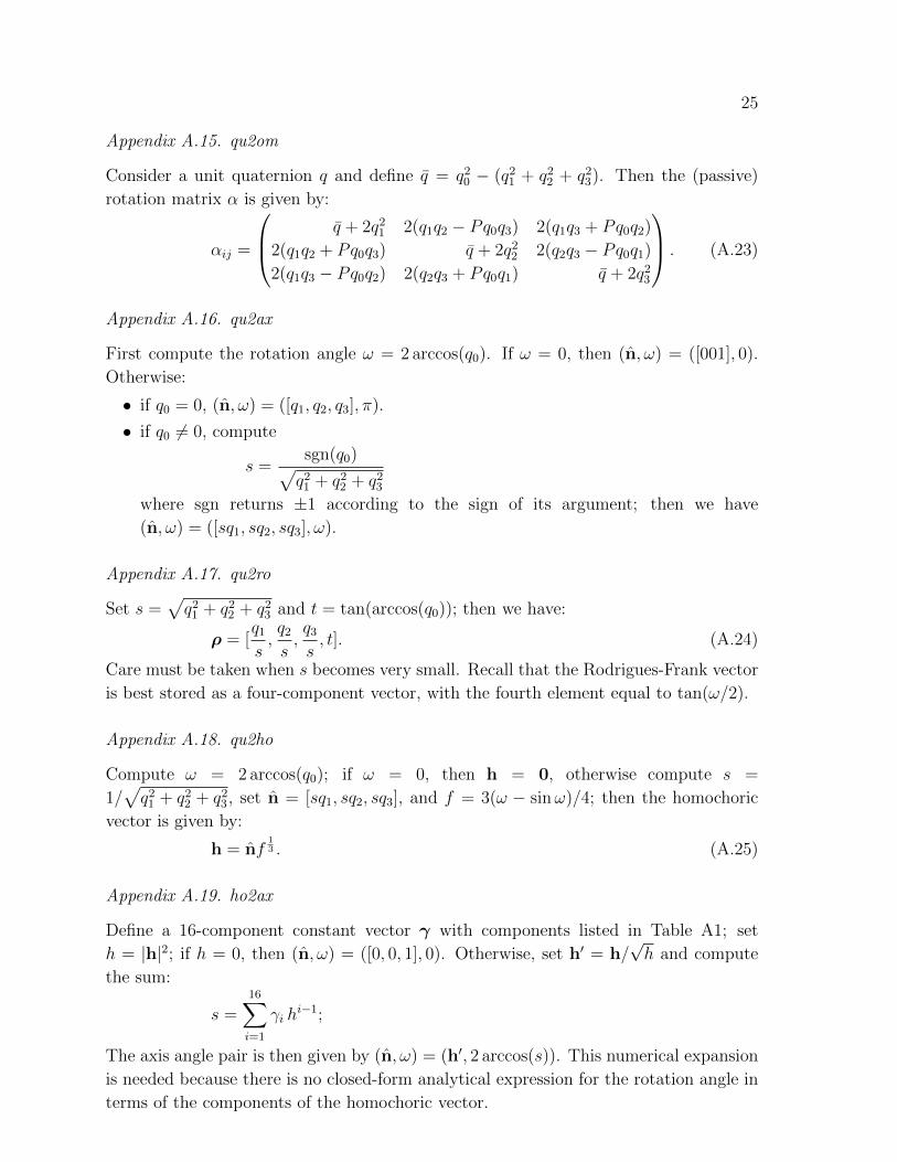
Appendix A.15. qu2om

Consider a unit quaternion q and define q = q20 − (q21 + q22 + q23). Then the (passive)

rotation matrix α is given by:

αij =

q + 2q21 2(q1q2 − Pq0q3) 2(q1q3 + Pq0q2)

2(q1q2 + Pq0q3) q + 2q22 2(q2q3 − Pq0q1)2(q1q3 − Pq0q2) 2(q2q3 + Pq0q1) q + 2q23

. (A.23)

Appendix A.16. qu2ax

First compute the rotation angle ω = 2 arccos(q0). If ω = 0, then (n, ω) = ([001], 0).

Otherwise:

• if q0 = 0, (n, ω) = ([q1, q2, q3], π).

• if q0 6= 0, compute

s =sgn(q0)√q21 + q22 + q23

where sgn returns ±1 according to the sign of its argument; then we have

(n, ω) = ([sq1, sq2, sq3], ω).

Appendix A.17. qu2ro

Set s =√q21 + q22 + q23 and t = tan(arccos(q0)); then we have:

ρ = [q1s,q2s,q3s, t]. (A.24)

Care must be taken when s becomes very small. Recall that the Rodrigues-Frank vector

is best stored as a four-component vector, with the fourth element equal to tan(ω/2).

Appendix A.18. qu2ho

Compute ω = 2 arccos(q0); if ω = 0, then h = 0, otherwise compute s =

1/√q21 + q22 + q23, set n = [sq1, sq2, sq3], and f = 3(ω − sinω)/4; then the homochoric

vector is given by:

h = nf13 . (A.25)

Appendix A.19. ho2ax

Define a 16-component constant vector γ with components listed in Table A1; set

h = |h|2; if h = 0, then (n, ω) = ([0, 0, 1], 0). Otherwise, set h′ = h/√h and compute

the sum:

s =16∑i=1

γi hi−1;

The axis angle pair is then given by (n, ω) = (h′, 2 arccos(s)). This numerical expansion

is needed because there is no closed-form analytical expression for the rotation angle in

terms of the components of the homochoric vector.

26

i γ4i+1 γ4i+2 γ4i+3 γ4i+4

0 1.000000000001885 -0.500000000219485 -0.024999992127593 -0.003928701544781

1 -0.000815270153545 -0.000200950042612 -0.000023979867761 -0.000082028689266

2 0.000124487150421 -0.000174911421482 0.000170348193414 -0.000120620650041

3 0.000059719705869 -0.000019807567240 0.000003953714684 -0.000000365550014

Table A1. Coefficients γi needed for the conversion from homochoric coordinates to

axis angle pair, described in section Appendix A.19.