•

July 1990 No. 320

DATA SOURCES FOR DEMAND ESTIMATION: TYPES AND FEATURES

By

Rueben C. Buse• University of Wisconsin-Madison

Rueben C. Buse is a professor , Department of Agricultural Economics , University of Wisconsin-Madison.

TABLE OF CONTENTS

DATA SOURCES FOR DEMAND ESTIMATION: TYPES AND FEATURES Introduction Types of Data . .

Time Series Data Cross Sectional Data Pooled Time Series and Cross Sections Panel Data . . . . . . . . . . . . . Scanner Data

Cross Sectional versus Time Series Comparisons Conceptual Issues . . Statistical Problems

Time Series Data Sets . . Disappearance Data Prices . . . . Income . . . . . . Major Cross Section Data Sets BLS Consumer Expenditure Surveys (CES/I, CES/ D) USDA Nationwide Food Consumption Surveys (NFCS) The National Health and Nutrition Examination Survey

(NHANES) . . . . . . . . . . . . . . . Panel Data . . .......... . . . . .... .

Continuing Survey of Food Intake by Individuals (CSFII) BLS Continuing Consumer Expenditure Surveys . University of Michigan Income Dynamics Panel Retirement History Survey (LRHS) Special University Panels Private Panels . . . . . . . . . Market Sales and Purchase Data Pragmatic Issues with Alternative Data Sources

LITERATURE CITED . . . . . . . . . . . . . . . . . . . . .

i

PAGE

1 1 2 3 5 5 6 7

10 10 13 15 15 16 17 18 18 20

23 24 25 26 27 27 28 28 30 31 34

DATA SOURCES FOR DEMAND ESTIMATION: TYPES AND FEATURESY

Intr oduction

A wide variety of data sets can be used in estimating and/or analyzing demand. They can be categorized in two dimensions, Cross sectional vs times series and experimental versus non experimental. Non-experimental cross sections and time series and variations on the two data types are the most frequently used data sets. The experimental approach systematically varies the independent variables of interest, such as price or income, and controls the influence of other exogenous variables on the dependent. Experimental data has fewer technical problems because of the controls on variation and covariation of the independent variables. In practice, the experimental approach has been limited to very specific research problems because of the difficulty of setting up reliable controls in real world situations at reasonable cost . There are no publicly available experimental data sets useful for demand estimation .!/ In contrast, no control is exercised over the variation in the independent or over their covariation in the non-experimental approach. The non-experimental approach uses whatever changes occur naturally in the environment from which the data is collected, recording the data expost . The majority of non-experimental data available are historical data series collected over time (time series) or surveys (cross sectional). The next section elaborates further on these two major data types.

Data series can also be classified as public or private according to the type of organization producing it and/or its general availability to the researcher . Public data sets are usually generated by government agencies and are readily available to the researcher at a small cost. In the United States, the most widely used and readily available public data used in demand analysis have been designed, developed and are maintained by the United States Department of Agriculture (USDA), the Department of Commerce through the Bureau of Labor Statistics (BLS), and special research studies by universities. Private data sets are generated as a source of income to private firms and are much more difficult to acquire, usually at substantial cost. Those data sets are usually special purpose and are not generally available for public research without cost . A number of both public and

~I This material is forthcoming as Chapter 8 in Market Demand for Dairy Products. D. Peter Stonehouse, Zuhair A. Hassan and S. R. Johnson. (Eds) . Iowa State University Press. Aines, Iowa.

!/ The rural income maintenance experiment and the New Jersey graduated work incentive experiment conducted by the Institute for Research on Poverty at the University of Wisconsin used the experimental approach to measure the impact of income support programs on work incentives. They are two of very few real world examples of the experimental approach in economic analysis and modeling . The data set does contain expenditures on housing, durables, clothing, health and a 24 hour recall of food intake (Bawden, 1970).

1

private data sets useful for demand analysis will be described in this chapter.

In almost all cases, whether public or private, the data was not designed for the purpose of using it in demand analyses . Therefore, in addition to describing the data series available for demand analysis it is also important that a potential user know more about the characteristics of the different types of data. In this chapter the next section elaborates on the characteristics of non-experimental cross sectional and time series data sets and section III examines conceptual and statistical issues in the various data types. Sections IV, V, VI, and VII are a detailed discussion of the various data sources and systems that are currently useful in demand analysis. The final section discusses some of the problems the user must be aware of in using the various data sets in demand analysis.

Types of Data

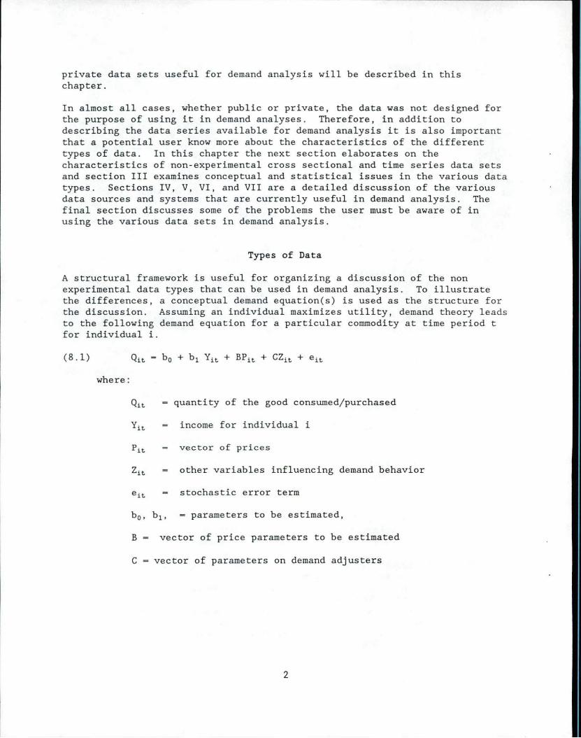
A structural framework is useful for organizing a discussion of the non experimental data types that can be used in demand analysis. To illustrate the differences, a conceptual demand equation(s) is used as the structure for the discussion. Assuming an individual maximizes utility, demand theory leads to the following demand equation for a particular commodity at time period t for individual i.

(8.1)

where:

Q1 t quantity of the good consumed/purchased

Y1t income for individual i

Pit vector of prices

Zit other variables influencing demand behavior

e 1 t stochastic error term

b0 , b 1 , - parameters to be estimated,

B vector of price parameters to be estimated

C vector of parameters on demand adjusters

2

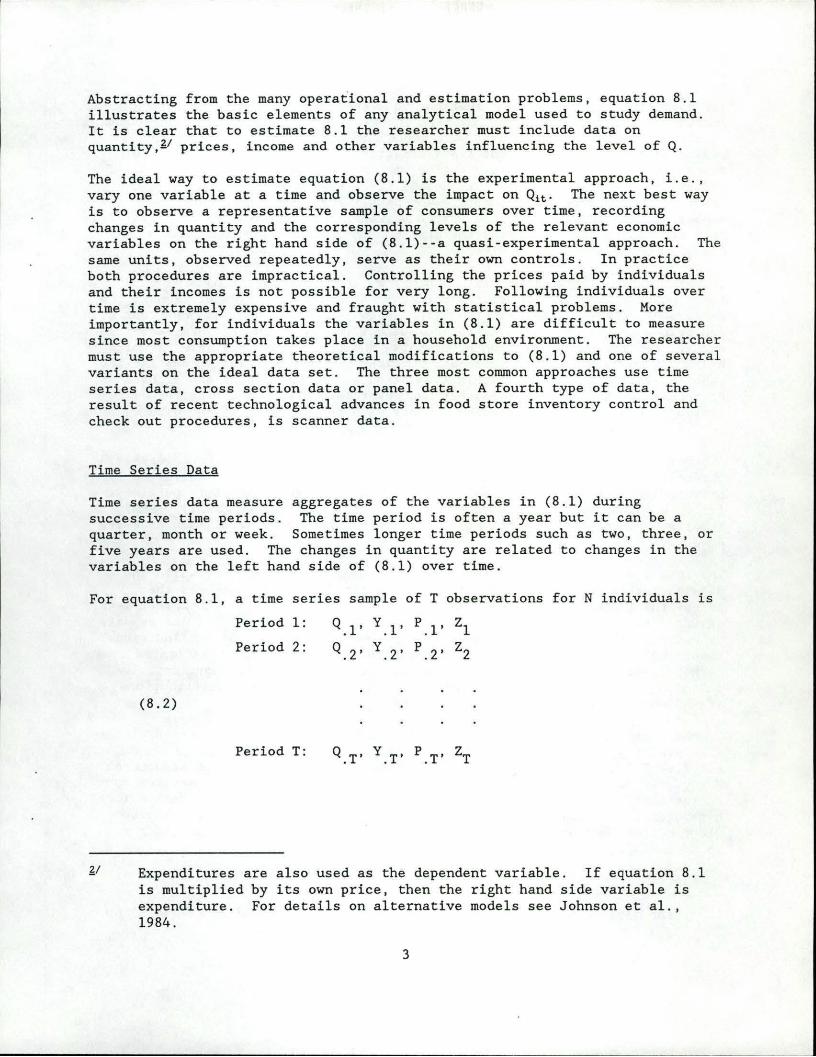
Abstracting from the many operational and estimation problems , equation 8.1 illustrates the basic elements of any analytical model used to study demand. It is clear that to estimate 8 . 1 the researcher must include data on quantity,~/ prices, income and other variables influencing the level of Q.

The ideal way to estimate equation (8 . 1) is the experimental approach, i . e . , vary one variable at a time and observe the impact on Q1t . The next best way is to observe a representative sample of consumers over time, recording changes in quantity and the corresponding levels of the relevant economic variables on the right hand side of (8 . 1)--a quasi-experimental approach. The same units, observed repeatedly, serve as their own controls. In practice both procedures are impractical. Controlling the prices paid by individuals and their incomes is not possible for very long. Following individuals over time is extremely expensive and fraught with statistical problems. More importantly, for individuals the variables in (8 . 1) are difficult to measure since most consumption takes place in a household environment. The researche r must use the appropriate theoretical modifications to (8.1) and one of severa l variants on the ideal data set . The three most common approaches use time series data, cross section data or panel data . A fourth type of data, the result of recent technological advances in food store inventory control and check out procedures, is scanner data .

Time Series Data

Time series data measure aggregates of the variables in (8 . 1) during successive time periods. The time period is often a year but it can be a quarter, month or week. Sometimes longer time periods such as two, three, or five years are used . The changes in quantity are related to changes in the variables on the left hand side of (8 . 1) over time.

For equation 8 . 1 , a time series sample of T observations for N individuals is

Period 1: Q . l' y

. l' p

. l' zl Period 2: Q. 2' y.2' p . 2' z2

(8.2)

Period T: Q.T' y.T' P. T' ZT

~I Expenditures are also used as the dependent variable . If equation 8.1 is multiplied by its own price, then the right hand side variable is expenditure . For details on alternative models see Johnson et al., 1984.

3

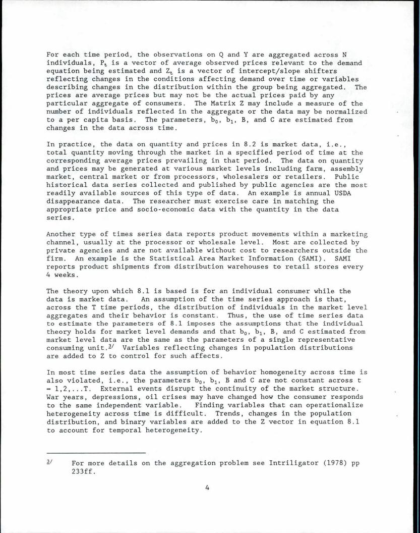
For each time period, the observations on Q and Y are aggregated across N individuals, Pt is a vector of average observed prices relevant to the demand equation being estimated and Zt is a vector of intercept/slope shifters reflecting changes in the conditions affecting demand over time or variables describing changes in the distribution within the group being aggregated. The prices are average prices but may not be the actua l prices paid by any particular aggregate of consumers . The Matrix Z may include a measure of the number of individuals reflected in the aggregate or the data may be normalized to a per capita basis. The parameters, b0 , b 1 , B, and Care estimated from changes in the data across time.

In practice, the data on quantity and prices in 8.2 is market data, i.e., total quantity moving through the market in a specified period of time at the corresponding average prices prevailing in that period. The data on quantity and prices may be generated at various market levels including farm, assembly market, central market or from processors, wholesalers or retailers. Public historical data series collected and published by public agencies are the most readily available sources of this type of data. An example is annual USDA disappearance data. The researcher must exercise care in matching the appropriate price and socio-economic data with the quantity in the data series.

Another type of times series data reports product movements within a marketing channel , usually at the processor or wholesale level. Most are collected by private agencies and are not available without cost to researchers outside the firm. An example is the Statistical Area Market Information (SAMI). SAMI reports product shipments from distribution warehouses to retail stores every 4 weeks.

The theory upon which 8.1 is based is for an individual consumer while the data is market data . An assumption of the time series approach is that, across the T time periods, the distribution of individuals in the market level aggregates and their behavior is constant . Thus, the use of time series data to estimate the parameters of 8 . 1 imposes the assumptions that the individual theory holds for market level demands and that b 0 , b 1 , B, and C estimated from market l evel data are the same as the parameters of a single representative consuming unit.11 Variables reflecting changes in population distributions are added to Z to control for such affects.

In most time series data the assumption of behavior homogeneity across time is also violated, i.e., the parameters b0 , b1 , B and C are not constant across t - 1,2, ... T. External events disrupt the continuity of the market structure. War years, depressions, oil crises may have changed how the consumer responds to the same independent variable. Finding variables that can operationalize heterogeneity across time is difficult . Trends, changes in the population distribution, and binary variables are added to the Z vector in equation 8.1 to account for temporal heterogeneity.

11 For more details on the aggregation problem see Intriligator (1978) pp 233ff .

4

Cross Sectional Data

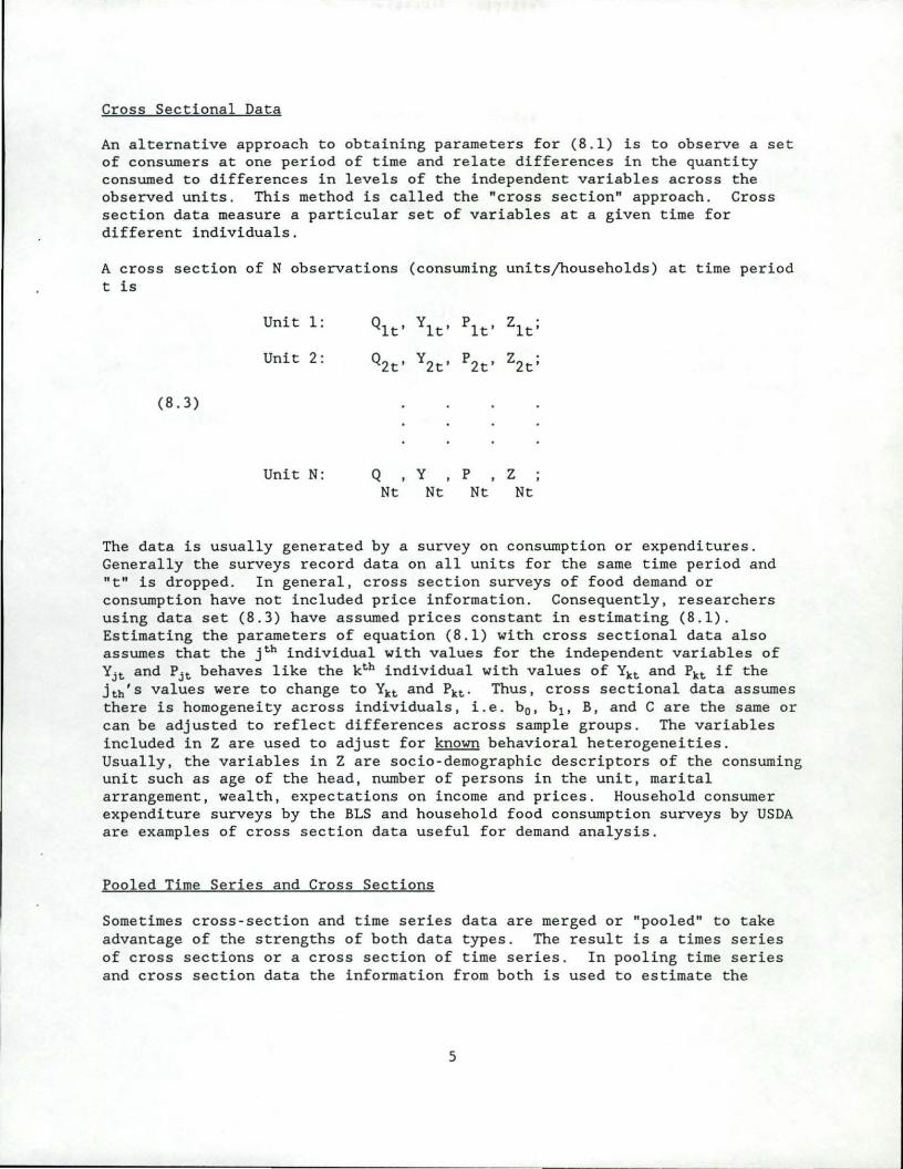
An alternative approach to obtaining parameters for (8 . 1) is to observe a set of consumers at one period of time and relate differences in the quantity consumed to differences in levels of the independent variables across the observed units . This method is called the "cross section" approach. Cross section data measure a particular set of variables at a given time for different individuals.

A cross section of N observations (consuming units/households) at time period t is

Unit 1:

Unit 2 :

(8 . 3)

Unit N:

Qlt' Ylt' Plt' zlt;

Q2t' Y2t' P2t' z2t;

Q y p z Nt Nt Nt Nt

The data is usually generated by a survey on consumption or expenditures. Generally the surveys record data on all units for the same time period and "t" is dropped. In general, cross section surveys of food demand or consumption have not included price information. Consequently, researchers using data set (8.3) have assumed prices constant in estimating (8.1) . Estimating the parameters of equation (8 . 1) with cross sectional data also assumes that the jth individual with values for the independent variables of Yjt and Pjt behaves like the kth individual with values of Ylct and Pkt if the jth's values were to change to Ylct and Plct· Thus, cross sectional data assumes there is homogeneity across individuals, i . e . b0 , b 1 , B, and C are the same or can be adjusted to reflect differences across sample groups . The variables included in Z are used to adjust for known behavioral heterogeneities. Usually, the variables in Z are socio - demographic descriptors of the consuming unit such as age of the head, number of persons in the unit, marital arrangement, wealth, expectations on income and prices. Household consumer expenditure surveys by the BLS and household food consumption surveys by USDA are examples of cross section data useful for demand analysis.

Pooled Time Series and Cross Sections

Sometimes cross-section and time series data are merged or "pooled" to take advantage of the strengths of both data types . The result is a times series of cross sections or a cross section of time series . In pooling time series and cross section data the information from both is used to estimate the

5

demand model. For example, the income coefficient (b 1 ) would be estimated from cross-section data conditioned on family size, race, education, and geographic location while holding (assuming) prices constant. Given the estimated income coefficient(s), times series data is used to estimate the demand parameters associated with prices . This method is sometimes used to remedy the multicolinearity problem among the independent variables in times series data.!/

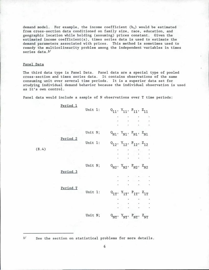
Panel Data

The third data type is Panel Data . Panel data are a special type of pooled cross-section and times series data . It contains observations of the same consuming unit over several time periods . It is a superior data set for studying individual demand behavior because the individual observation is used as it's own control.

Panel data would include a sample of N observations over T time periods:

Period 1 Unit 1:

Unit N;

Period 2 Unit 1 :

(8 . 4)

Unit N;

Period 3

Period T Unit 1:

Unit N;

! / See the section on statistical problems for more de tails.

6

Panel data useful to demand analysts are not widely available since they are expensive to obtain and usually designed for particular research objectives . The major difficulty with a panel is sample attrition, i.e., with each succeeding time period a percentage of units drop out of the survey because they stop cooperating, move, or otherwise disappear. In practice, "pseudo panels" are often used. In the pseudo panel their is no attempt to maintain the individual units in the sample over time. In this approach, a set of consuming units is observed and measured at one or more time periods and then replaced by comparable units . In either case, the problems of panel data are a combination of those of both time series and cross sectional data.

Using data set (8.4) the coefficients on the explanatory variables in 8.1 are subject to both time and individual effects . The researcher using panel data must include variables in Z that allow for the possibility of differences in behavior over cross-sectional units as well as differences in behavior over time for a given cross sectional unit . The appropriate variables and estimation procedure depends upon the researchers maintained hypothesis on those coefficients . One can assume they vary over indiv iduals, over time, or both (binary variable models) . Alternatively , one can assume model coefficients are random variables with components for individuals, time or both (error-components model).11

The oldest nationwide household panel is the MRCA-Panel developed by the Market Research Corporation of America. It is a private data set originally established in 1939. The most recent public panel data is the BLS Consumer Expenditure Survey begun in 1980. It is a "pseudo-panel" in that household rotate out of the sample and are replaced periodically .

Store panels are another type of panel data . Continuous data from a sample of retail stores was developed because of the high cost of household panels . The A.C. Nielsen company is a private company reporting data on sales of food chains obtained via store panels . In this approach store sales are audited every 60 days to obtain information on product sales during the past 30 days. The results measure retail sales by determining the quantity of product delivered to the store. The Q1 is sales per product or brand per store per time period . There is no accompanying data for Y and Z. The data is summarized by regions of the U.S., by SMSA and by population size. The necessary supplementary socio-economic data can be obtained from sources such as census or population surveys .

Scanner Data

The fourth type of data, scanner data, is relatively new and has been rarely used in demand analysis.~/ Scanner data is an outgrowth of new technologies

11 The reader is referred to chapter 8 of Judge et. al . , (1980) for details .

~I See Capps 1987, for a review of recent literature on using scanner data in demand analysis.

7

to increase the efficiency of food stores by using Universal Product Codes (UPC) and scanners at the checkout counters. The UPC and retail point of purchase scanning systems produce a wealth of new data that can be used in demand analysis. A given 11-digit UPC code represents a specific manufacturer/size/flavor/color or other related information. Point of purchase scanning can provide information on a weekly, daily or even hourly basis. The transaction recorded by the scanner typically includes the UPC code, time of transaction, the units of the sale and price per unit . The total value of the sale may or may not be included in the data but is easily obtained from the recorded data.

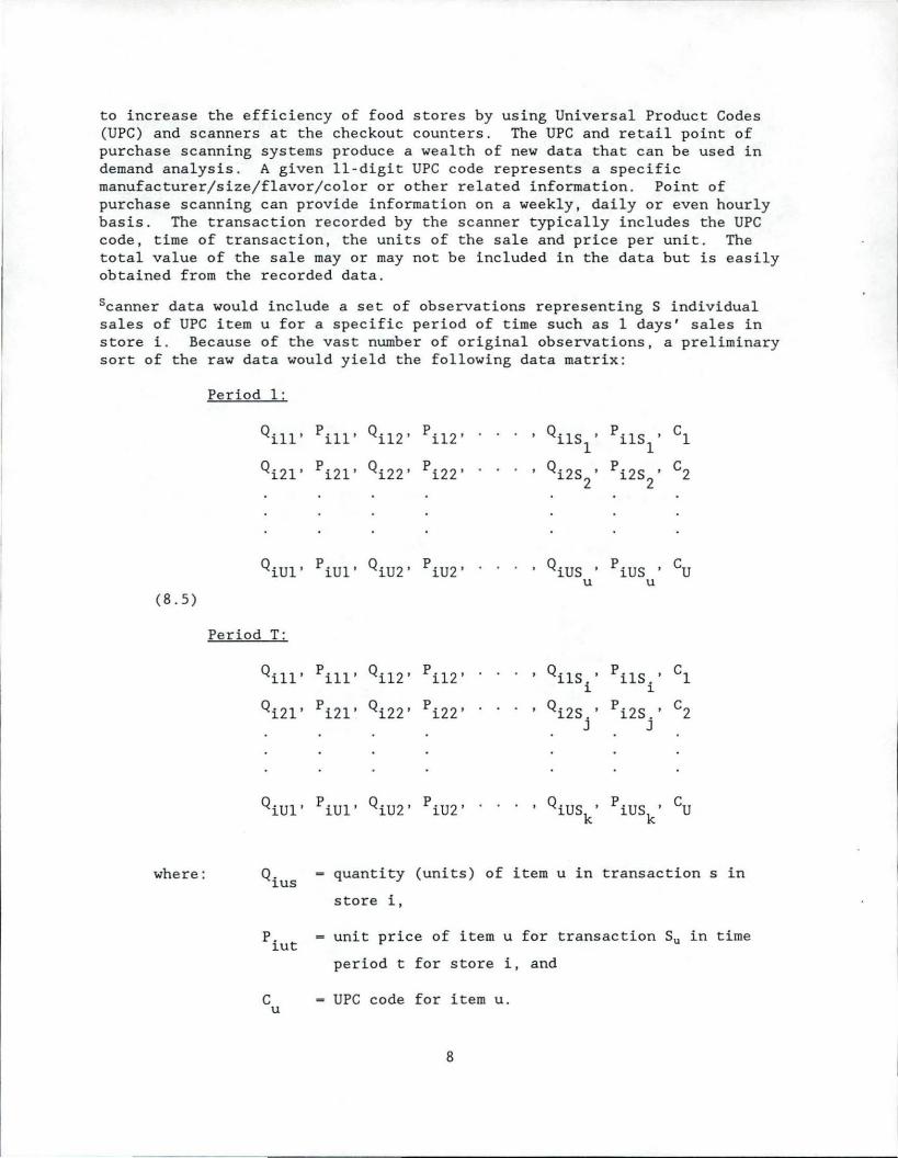
5canner data would include a set of observations representing S individual sales of UPC item u for a specific period of time such as 1 days' sales in store i. Because of the vast number of original observations, a preliminary sort of the raw data would yield the following data matrix:

Period 1:

Qill' pill' Qil2. p il2. . QilS ' p ilSl' cl 1

Qi21' pi21' Qi22' pi22' • Qi2S ' pi2s2

• c2 2

QiUl' p iUl. QiU2' piU2' . QiUS . piUS . cu u u

(8.5)

Period T:

Qill' pill' Qil2' pil2' • QilS.' l.

pilS.' l.

cl

Qi21' pi21' Qi22' pi22' • Qi2S.' p i2S.' c2 J J

... '

where: quantity (units) of item u in transaction s in

store i,

P. - unit price of item u for transaction Su in time l.Ut

period t for store i, and

C UPC code for item u. u

8

Note that within a time period the number of transaction will be different for each UPC code, S1 ~ S2 ~ . . . Su ~ Si ~ SJ ~ .. . Sk . Note also the greater detail on food items available in scanner data . Demand analysis is possible on any one of the more than 40,000 UPC codes . Large stores will use 35 , 000 to 40,000 different UPC codes and smaller stores 10,000 to 15,000. There can be many UPC codes for any particular food. Since stores do not ordinarily change the price of a specific product on a daily basis, the price associated with a group of transactions (Piu) will be the same. The recent advent of electronic pricing is likely to produce scanner data with more frequent price changes.

If desired, the data for an individual store can be aggregated to the city, region or chain level . Thus a complete machine-readable diary of sales for a given food category are available for all brands/types/etc. as well as for complementary or supplementary products. This type of data can provide insights into the demand for specific products as affected by price, coupons , advertising and promotion , shelf space , etc., variables that are not available with other data types. Generally the additional variables can be obtained from other sources within the outlet .

The major problem with scanner data is data overload . The scanner data records every sale of item u on a daily basis . Thus one day's data can easily include tens of thousands of transactions ranging over more than 20,000 items in a typical retail food store. Eliminating unwanted UPC codes, sorting, aggregating across Qi and otherwise sununarizing the raw data is a non-trivial research problem.

The data set (8.5) does not include Y or Z for the individual making each purchase . For traditional demand analysis the data needs to be supplemented with other data before estimating equation (8.1) . Scanner data contains substantial variability due to supplemental, complementary and competitive promotion programs, seasonal and day of the week effects, nearness to payday, weather, holidays, and other "outside" factors influencing consumer purchase behavior. Variables to reflect such "exogenous" factors can be incorporating in the data from other sources . Alternatively, the maintained hypothesis implied by omitting Y and Z must be clearly examined . Some researchers argue that, for a particular store or group of stores, scanner data represents a quasi-controlled experiment . Assuming the socio-demographic variables of store patrons are constant, once the consumer is in the store, the only constraint on behavior is the economic constraint of relative retail prices (Wisniewski (1984). If true, store scanner data is optimal for standard demand curve estimation. Funk, Meike and Huff (1977), Jourdan (1980), and Marion and Walker (1978) have calculated price elasticities from scanner data . Up to the present there are no publicly available scanner data sets. Most large food chains have developed their own proprietary data but it is available only through cooperative agreements with specific firms . Branson argues that scanner data combined with a consumer panel has great potential in that is reduces measurement error (Branson et al., 1987). "Behaviorscan" by Information Resources Inc. links scanner equipped stores to a household panel.

9

Cross Sectional versus Time Series Comparisons

The two most readily available data types are time series and cross sectional data . Each has advantages and disadvantages, impose different assumptions on the data and the econometric model, and hence, on the interpretation of the estimated parameters of (8 . 1). Panel data generally incorporates features of both times series and cross sections . This section discusses and contrasts some of the conceptual differences and statistical problems in each .

Conceptual Issues

Clearly , the fundamental difference between times series and cross sectional data sets in estimating demand parameters is the time period spanned by the data . Both approaches also impose strong assumptions on the data. First, the maintained hypothesis with respect to how the independent variables affect demand behav ior are very different . With time series data the independent variables change over the time frame of the data set while in cross section data, the variables change across the consuming units within a time period . In addition, the characteristics of Qi t and Pit are assumed to be homogeneous across all t. In practice, new technolog ies lead to product improvements that give consume rs greater satisfaction , perhaps at the same price as the less improved product or the Qit purchased at Pit by high income consumers is of higher quality than that same quantity purchased by a low income consumer. Thus the demand equation 8 . 1 may be measuring diff erent products across time in the time series data or across units in the cross section data .

Secondly, researchers find that times s e ries and cross section data yield different estimates of a demand model . In general the estimated income elasticities of demand using cross section data are greater than those obtained using time series data. Time s series estimates of 8 . 1 reflect short run behavior while cross section estimates reflect long run equilibrium behavior.II The behavior homogeneity assumption implies that a relatively poor family would consume the same amount of a commodity as a rich family if its income were to become as large . Howev er the poor family requires time to change its consumption levels as its income grows . Consequently it is only in the long run that a poor family's data will reflect a consumption pattern similar to the high income family .

Third, because of the variables avai l able in each data type, both approaches impose additional structure on the data environment. In cross sectional data the observations are taken over a short period of time. Hence, the consuming units are frequent l y assumed to face the same set of prices, even when the sample units are spread across the U.S. The price effects are collapsed into the constant term, b 0* - bO + BPit· In time series the counterpart assumption

l l See Meyer and Kuh (1957) for further discussion. Kuznets (1966) says it is inappropriate to use cross section data to make inferences about pas t long- term trends . For forecasting purposes time series data is most appropriate.

10

of constant prices is that the characteristics of the households in the aggregates do not change over time. Average age, family size, marital status, wealth, or other socio-demographic characteristics affecting demand change slowly and are usually omitted from the Z vector. The high degree of multicolinearity of such variables is another reason for their exclusion from the statistical version of (8 . 1) . They are usually replaced by a single time trend.

Fourth, the usable degrees of freedom differ substantially . The sample size of times series data is small in comparison to cross section data. Annual data on the supply and disappearance of foods and market prices have been collected on a systematic and consistent basis since the early 1930's. In practice, most analysis use data since World War II yielding a maximum of 40 annual observations . In some cases time series are available on a quarterly basis . Thus the maximum number of data points in about 160 . In contrast, one can easily find cross section surveys of thousands of sample units. But the large number of individual observations requires more Z-variables to account for inter-unit heterogeneity . In cross section surveys, the number of useful observations is inversely related to the number of independent variables in 8.1. Missing data on the independent variables, particularly income, can reduce the number of useful observations. The end result of the reduced sample may be estimates of (8.1) which are not representative of the overall sample .

Fifth, the sources of variation in Q across the observations is much greater in cross sections than in time series and the explained variation is much lower. Coefficients of multiple determination for equation 8.1 for time series data are generally several magnitudes larger than for cross section data, e . g .9 or larger for time series vs . 3 or less for cross section data. The error term in 8 . 1 is the result of measurement error in Q, omitted variables on the right hand side of 8 . 1, and stochastic behavior of the units of measurement . In time series data, some part of the stochastic variation in individual behavior and measurement error is averaged out in the aggregation process. As a consequence, explainable variation is a larger part of total variation. In cross section data the variation in Q from observation to observation contains all three sources plus a larger random component due to individual idiosyncracies .

Sixth, the amount of detailed information in micro data sets is much greater than in time series data. In cross section data values on Qi are usually reported for detailed foods rather than the large aggregates of historical time series. For example, using cross section surveys it is easy to model the quantity demanded of particular cuts of beef, pork or whole vs cutup poultry. In contrast the finest level of detail in the disappearance data published by USDA is for Beef, Pork and Poultry. It is possible to combine the detailed Qi in cross section data with time series data to analyze a system of demand equations in a stagewise demand system.

Seventh, there is greater variation in prices in time series data than in cross sections. In fact, cross section data generally does not explicitly include price information. Up until recently, researchers assumed that, because of the short time span of the inquiry, all sampled units faced the

11

same set of prices. Recent studies by Buse et. al, Cox and Wholgenant, and Kokowski demonstrate that prices are important explanatory variables. Prices can be incorporated into the data set by either using published price series (Buse; KoKowski) or implicit prices obtained from the unit's reported expendi tures (Cox and Wohlgenant). Implicit prices in cross section data can be difficult to interpret. For example, do price variations reflect real differences in supply of a homogeneous product or differences in product quality?

Eighth, it is difficult to reconcile the data from a representative cross section sample with its time series counterpart or to relate (8.1) back to farm level demand. Swnming the appropriately weighted quantities in (8.3) does not equal the corresponding quantity in (8.2):

(8.6) N L;

i-1 W.Q. "'

1. 1. t

where: wi the appropriate expansion weight for the j th unit, Quantities in (8.3) , and Quantity in (8.2).

There are several reasons. First , time series data from 8 .2 is an aggregate measures of total demand for all uses . In comparison, cross section data produce an incomplete picture of demand. It does not account for all end uses. Generally institutions such as hospitals, military and penal installations , schools and similar institutions are not represented in consumption or expenditure surveys . Second, food eaten away from home is reported as an aggregate value rather than as quantities of beef, pork or milk consumed away from home. It is also hazardous to try and relate cross sectional models back to farm leve l demand because the institutional and technological conversion factors involved in converting a farm product into the product on the consumers table are mainly unknown. In addition, researchers find there is a tendency of households to underreport certain types of expenditures (Gieseman, 1986; USDL/BLS, 1986 and over reporting on others (Rathje 1984). To a lesser degree, the same problem is inherent in time series models estimated from aggregated retail disappearance data. Many primary farm products involve unknown combinations of many end uses. For example, fluid milk is converted into many distinct dairy products. The farm leve l quantity of highly processed products is difficult to calculate because of processing waste, non-food uses of parts of the primary product, general waste and other losses.

Finally, missing or incomplete data is a minor problem in time series. In cross section data it can become a major problem. It is very likely that some observations will be missing values of dependent or independent variables. For the dependent Q1 , some surveyed units do not purchase or consume a particular food item. Because of their purchase patterns others do not repor t purchasing or consuming in the survey period. In either case , the researcher must decode whether to exclude such observations or use probit or tobit procedures t hat takes into account such behavior. Missing information on the

12

independent variables may be simply a non-response or protecting data due to confidentiality concerns, e.g. top coding very large incomes. If there is missing data the observation is usually dropped from the analysis.~/ Dropping observations can produce biased coefficients in (8.1), if the "missing data" observations are not distributed randomly across the population. It is difficult to interpret the statistical results without extraneous information on the sign and magnitude of the bias.

Statistical Problems

All types of data are susceptible to particular statistical problems. In time series, autocorrelation and multicolinearity complicate the computations. In cross sections the problem is more likely one of heteroscedasticity of the error term, eit• and zero values on Q. In panel data it is a combination of all the problems. There has been so little experience with scanner data in demand analysis that there is no literature on statistical problems peculiar to such data. Nevertheless, they surely exist and will be appearing in the literature in the near future.

Time series data exhibits serial correlation of the residual and correlation among the independent variable. The model variables tend to change in a similar pattern from one time period to the next because the general level of economic activity affects all the variables in the model. Since the error term reflects conditions not explicitly accounted for in the model (e. g. omitted variables), first order autocorrelation in the residuals is also usually encountered.

Time series data also exhibits multicollinearity for the same reasons, i.e., the tendency of the independent variables to move together. For example income and prices exhibit the same cycles and trends over time. Thus there may be too little independent variation to accurately calculate the affect of the independent variables on the dependent, ceteris paribus. All four types of data can suffer from small independent variation in the independent variables making it difficult to estimate particular parameters accurately. It is usually the most serious in time series data, although price in cross section data will also exhibit a high degree of multicolinearity.

Another problem with time series, cross sectional and panel data is operationalizing known structural change. The change may be because of shifts in consumer behavior or because of changes in the data generation process. If the demand structure has changed then, at two different points of time, the data reflects different behavior by the same consumers. For example following world war II consumers reacted differently to price and income change than before Pearl Harbor. Similarly, there is research evidence that the consumer's response to price changes following the oil crises of the early 1970's is different than before the change but exactly where and how the behavioral change took place is not clear . Recent public health information

~I There are other methods of adjusting for missing data. For details see Stonehouse et al., Chapter 7.

13

on diet has changed the consumers attitudes towards foods such as poultry, fish, dairy products and red meat. Finding the appropriate variable to reflect the new information on diet and health to incorporate into equation (8. 1) is difficult. A change in data conceptualizations of those who collect and publish the data is a second type of structural change, i .e., in time series, the data may have been revised. The problem is that improved conceptualization is reflected in the published data but the exact nature of the revision may not be either known or published. A change in data coverage is a third possibility. For example, between 1981 and 1983 the BLS consumer expenditure panels did not sample r ural areas.

Heteroscedastic error terms are the major statistical problem of cross sectional data. The heteroscedasticity arises our of the fact that the errors are related to household characteristics in the Z matrix. For example, low income households have less income to allocate across foods than high income households. As a consequence there is more choice and variation in Q1 for high income households. Since income is highly correlated with other socio­demographic measurements, the error variance is usually related to many of the socio-demographic characteristics of the consuming unit. Again, the most appropriate correction is unresolved.

Multicolinearity among particular subsets of variables such as age, income and education can also be a problem in cross section data. Multicolinearity increases the difficulty of testing hypothesis on the parameters. Income is generally highly correlated with age and education, making it difficult to obtain statistically reliable results. The more socio-economic variables included in Z the more complex is the multicolinearity . If prices are incorporated into a cross sectional analysis they also are highly intercorrelated.

Errors in measurement can also be sever e in cross section data sets. The var iables are usually based on the interviewees recall or recording ability. Research indicates that many variables in micro-data sets contain substantial measurement error since most statistical estimation procedures assume the independent variables are measured without error. Such errors can subs tantially affect the estimates. Duncan and Hill (1984) illustrate the magnitude of the problem using respondents recall of labor earnings. Altonje and Siow (1987) show the affect on the consumption function of measurement error in income.

Zero values for the dependent variable is another statistical problem in cross section data . For highly disaggregated demand analysis a certain percent of the respondents will report a quantity of zero. The zero can be interpreted as not ever consuming that food item, or not consuming or purchasing in the period of inquiry (e.g. yesterday, last week or month). In e ither case the data is said to be censored at zero. The econometric implications of a censored data set are beyond the scope of this chapter but require estimation procedures other than OLs .21 There is an alternative approach to circumvent

21 See Maddala for a detailed discussion of appropriate estimation procedures.

14

zero values on the dependent variable. This approach subsets the data into groups of similar types of units, such as all single person households, all two person households aged 25 to 35, all households aged 36 to 55, etc. The procedure uses mean expenditures and income for each socio-economic cell to estimate the parameters of 8 . 1. Using cell averages or aggregates requires assuming micro behavior and average macro behavior are equal. Using group averages also introduces a weighing problem. Each cell likely contains different numbers of units and thus different amounts of information are included in the aggregates of each cell. The estimation procedure must account for those differences if the estimates are to have desirable statistical properties. 101

Panel data can exhibit both autocorrelation and heteroscedasticity. The error variance of the sample of observations may be different across both time and the units . For example, the error variance of an individual for one time period may be about the same as for the next period. Thus, the error variance of e 1t across time will be correlated. Simultaneously, the error variance of an individual observation may be related to the income level of that unit. If the error variance of e 1t are heteroscedastic and autocorrelated, classical least squares is not appropriate to estimate the parameters of (8 .1).

Time Series Data Sets

Almost all time series data used in demand analysis of agricultural commodities is collected and published by USDA and BLS. It is a byproduct of their responsibilities and, as such , its "match" to the economic concepts implied by the theory of (8.1) is imperfect . The time series counterpart of Q1 is USDA Disappearance data . For prices, P1 , there are several alternative price series.

Disappearance Data

The disappearance data is the most comprehensive measure of the consumption and utilization of domestically produced food in the United States. It measures domestic market supply in a given time period . The time period for most commodities is annual, although a few commodities are estimated for shorter periods. The length of the time series varies by commodity with the longest period being since 1909. Currently the disappearance data includes more than 200 individual agricultural commodities.

USDA regularly produces estimates of supplies of domestically produced agricultural products. Food disappearance quantities are calculated as a residual from total estimated production adjusted for stock changes, imports and exports, nonfood and non-market uses . .ll/ The residual is converted from

lO/ See Stonehouse et al. , Chapter 7 for details .

.ill For details on the procedures see USDA 1988.

15

a primary commodity weight (e.g., carcass weight, fluid milk equivalent) to the retail weight equivalent. Retail weights of farm level commodities are difficult to calculate because many of the institutional and technological conversion factors are not precisely known. Processing waste, nonfood uses of parts of the farm product, other wastes and losses in marketing and storage are examples of the factors that must be subtracted from farm level production to obtain retail weights. 121 The estimated retail weight is divided by estimated civilian population to obtain annual per capita disappearance or consumption. The primary use of this data is to provide a description of the flow of U.S. produced agricultural commodities into end uses. Since it measures total disappearance it includes both at-home and away-from-home consumption. If it is assumed that the commodity market in question is in equilibrium over the observational period, the disappearance is conceptually equivalent to the quantity clearing the market at prevailing prices.

The data is published regularly in USDA's Agricultural Statistics and in its annual statistical bulletin, Food Consumption. Prices and Expenditures. 131

Prices

Prices are published at several levels of the marketing system. It is important to match the disappearance data with the appropriate price . State and national farm level commodity prices as of the 15th of the month are reported in Agricultural Prices . They are based upon a survey of commodity dealer's prices paid to farmers . The prices are representative of the average quality sold by farmers at the first level of sale. The Agricultural Marketing Service also reports prices by grade and variety on designated central wholesale markets in commodity publications. Wholesale prices are also collected for many products by the Bureau of Labor Statistics. Individual product prices and product group prices are reported monthly in the Survey of Current Business .

Consumer prices are gathered and published on both a monthly and annual basis by the Bureau of Labor Statistics in the Consumer Price Index (CPI). For analyzing the demand for food most researchers use the consumer price index for all urban consumers (CPI-U) or the CPI for wage earners (CPI-W). The CPI­W has been published for more than 50 years. It covers urban hourly wage earners and clerical workers in the civilian noninstitutional population. The CPI-Uhas been published since 1978 . It is a broader index in that it covers all residents in urban places . It is widely used as a general measure of inflation.

The CPI-U is a statistical measure of price changes for a set of goods and services included in a representative "market basket". It measures retail prices for about 80% of the U.S. civilian population. Currently it is

121 For an example of the problems in deriving retail weights see Nelson and Duewer's (1986) discussion for red meat.

13/ As an example s ee USDA (1987).

16

published monthly for 28 major cities, for regions and various sizes of urban areas and a national average. The city and regional CPI measures changes in specific cities, urban areas or regions over time but cannot be used as a measure of price differences among locations . 141

The CPI includes prices for 16 major food groups including food at home , cereals and bakery products, beef and veal, pork, other meats, poultry, fish and seafood, eggs, dairy products, fresh fruits and vegetables, processed fruits and vegetables, sugar and sweets, fats and oils, nonalcoholic beverages, other prepared food, and food away from home. Prices are also published for a number of specific sub items within each of the food groups. For example, in addition to a price series for beef and veal, prices are collected and published for ground beef, chuck roast, round roast, sirloin steak , and other beef and veal. The two series also include prices for all the nonfood components of the market basket.

The BLS also publishes monthly producer prices for 15 different food groups . The producer price indices reflect price changes at various levels in the production and marketing channels .

A major problem with matching price data with disappearance data is that there is no close correspondence between the quantity in the USDA disappearance data and reported prices . The quantities in the disappearance data are "retail weight equivalents" . They are indirect estimates of the actual consumption at the retail level while the price data is for actual retail quantities at retail stores. The quantity measures total vo lume i.e . beef, pork or vegetables moving into consumption while the reported price is for a specific item such as the weighted retail price of beef or a price for sirloin steak, ham , or frozen vegetables.

Income

Income is included in (8.1) to measure changes in the purchasing power of consumers . A frequently used income series is per capita disposable income as calculated from the national accounts. It is published annually and quarterly by the U.S. Department of Commerce in The Survey of Current Business. If a more detailed breakdown of income i s desired, t he Bureau of the Census annually estimates the per capita income of families and individuals . Specific estimates are provided for different regions , ethnic groups, occupation, household types and ages on a national basis.

141 For more details see Blanciforti and Parlett (1987).

17

Major Cross Section Data Sets

The following describes the des ign of and information contained in recent surveys of U. S. households that are useful for demand analysis. They include data on food consumption or expenditures. The surveys described are:

1. Consumer Expenditure Surveys (CES), 2 . Nationwide Food Consumption Surveys (NFCS), 3. National Health and Nutrition Examination Surveys (NHANES),

These micro data sets are very large, ranging from several thousand to tens of thousands of observations. Information on how to obtain machine readable data can be obtained from the National Technical Information Service of the U. S. Department of Commerce or the Division of Consumer Expenditure Surveys of the BLS .

BLS Consumer Expenditure Surveys (CES/I, CES / D)

The consumer expenditure surveys are conducted by the Bureau of Labor Statistics . It is responsible for publishing the nation's price indices and the periodic surveys provide the basic information used in calculating the weights for those indices. The surveys collect detailed information on the income, expenditures and financial status of a representative sample of U.S . Households. There have been surveys in 1888-91, 1901, 1917-19,1933-36, 1941 -42, 1950, 1960-61, 1972-73 and on a continuous basis since 1980. 151 The first survey obtaine d cost -of-living data from U.S. Wage earners. Subsequent s urveys were of wage earners and salaried workers in urban areas . Starting with the 1960-61 survey both the scope and sample were e xpanded . It now samples the entire non- institutional population of the United States. In addition to the data required for expenditure weights, the 1960-61 survey collected information on household socio-demographic characteristics, assets and liabilities, and income. The 1960-61 survey used a 7-day recall for food expenditures and a longe r recall period for other expenditures. The recall methodology provided very little de tail on food expenditures and the accuracy of recalling past purchases was questioned. As a result , the methodology of the succeeding 1972 -73 and later surveys was changed.

Starting with 1972-73, BLS used two separate surveys, each with their own questionnaire and sample. The rational was that the recall of expenditures varied with the cost and importance of the item. Information on large more easily reca lled expenditures such as housing, utilities, clothing, furniture, appliances, health care, recreation, transportation and educational expenses were collected in a series of 5 quarterly interviews covering a 15 month period. This survey is commonly referred to as the Interview (CES/I). The CES/I also obtained global estimates for more frequently purchased items such as expenditures on food, beverages, and utilities. The CES/I was designed to obtained detailed information on 60 to 70 percent of a households expenditures and aggregate information on another 20-25 percent. The details on those

ill For a detailed history of the early surveys see Carlson (1974).

18

global aggregates of frequent purchases and any remaining expenditures were obtained in the second concurrent survey, the Diary survey (CES/D).

The CES/D collected information via a dail y diary on the 30 to 40 percent of total expendi t ures that are most frequently purchased. Participating households were requested to keep a detailed diary of purchases over two consecutive one-week periods . The expenditure components covered by the diary are food, household supplies, personal care products and non-prescription drugs . The BLS publishes expenditures for more than 50 different expenditures from the interview and for 20 different foods from the diary. In addition BLS publishes integrated data from the interview and diary.ll1

Up until 1960-61 the data was only available from BLS as published in its statistical bulletins. The 1960-61 survey marked the first time the BLS released the microdata in machine readable form (magnetic tape). Data from all BLS expenditure surveys since 1960-61 are available in machine readable format. The level of expenditure detail and socio-economic information in those tapes can be overwhelming. The detai l tapes contain information on thousands of different expenditures and on the characteristics of each member of the sampled unit.

Sample Design: The sample design of surveys prior to 1960-61 varied from survey to survey . Generally they concentrated on urban areas. In some surveys the CES was augmented by the USDA's survey of farm families. The 1960-61 survey sampled both rural and urban areas of the U.S . It included 13,728 usable schedules . The 1972-73 and later surveys sampled the noninstitutional population of the United States and include all urban, rural, farm and nonfarm households . The 1972-73 interview sample size was 19,975 consumer units and the diary sample was 23,186.

Data: In addition to expenditure data all surveys collected information on the household's socio-economic characteristics . The more recent surveys contain a wider variety of information than the earlier surveys. Both the interview and the diary collect detailed information on the socio -economic characteristics of the consuming unit, 171 e.g. , age, sex, race, education and marital status of each member; location, housing and tenure (owner/renter); and occupational characteristics of head and spouse. Both instruments also collect details on the consumer unit's income--including in­kind income and a set of questions on food stamps. Because of differences in collection methods, the income reference period in the CES/I is not the same as for the CES/D. The diary reference period was the previous 12-months while the survey reference period was the calendar year. As a further difference, diary incomes cover varying 12 month reference periods .

16/ See BLS Bulletin No . 1992.

171 The terms "household" and "consumer unit ' are used interchangeably . However, the consumer unit is the most appropriate term. The exact definitions are in the BLS Handbook of Methods, Bulletin No . 2134 , 1984 or BLS Bulletin No. 1992, 1978.

19

In the (CES/I) each CU is queried in detail about all its' periodic expenses. The interview expenditures cover clothing, utilities, furniture, large and small appliance, real estate, motor vehicles, information on out of town trips and vacations, taxes, repairs , insurance, professional services and contributions. In the available detail tapes expenditures for each consumer unit are recorded for more than 3,500 different items. In addition, global estimates of expenditures on food at home, food away from home, alcoholic beverages, drugs, medicines, and personal care are also obtained . These latter items are covered in detail in the CES/D.

The interview (CES/I) also includes a detailed inventory of major durable goods such as automobiles, stove, dishwasher, etc; characteristics of those durables such as whether the automobile had air conditioning or a standard transmission, the refrigerator is frost free, etc; an inventory of minor appliances, and assets and liabilities of the CU. The information on sources of income is also more detailed than in the CES/D .

The major components of the diary (CES/D) include food, household supplies, personal care products, non prescription drugs, and housekeeping and garden supplies . Within each broad category a very detailed set of items are available. For each individual or consuming unit it can include several thousand different items such as wheat flour, t-bone steak , 2-percent milk, canned vegetables, vacuum bags, new appliances, used appliances, books, magazines, power tools, water softening service, motor oil, and cooling system repairs. In all, more than 1700 different expenditures are recorded ~ith more than 1200 for food. The recorded expenditure may be for either 1 or 2 weeks .

Although expenditures are recorded, there is no explicit price information included in the BLS data surveys. This is a major limitation for the researcher interested in demand analysis since the assumption of constant prices across the time frame of the more recent surveys is questionable . For food, there has been some work on estimating price information from the quantities and total expenditure data, when both are available. 181

Obtaining food quantities from BLS tapes requires a substantial amount of preprocessing and data cleaning. 191

USDA Nationwide Food Consumption Surveys (NFCS)

The USDA has conducted national surveys of food consumption about every 10 years. These surveys provide information on the quality of diets and the amount of money spent on food by U. S . households . Surveys were conducted in 1936-37, 1942 (spring only), 1948 (urban areas only) , 1955 (spring only), 1965-66 and 1977-78 . The first four surveys included detailed information on household food use . Later surveys were expanded to include information on food consumed away from home and to seasons other than the spring quarter . In

181 See Capps and Havlicek (1981).

1.21 See Capps, Spittle and Finn (1981) for details on obtaining implicit prices from the 1972-73 BLS/D.

20

1965-66, data was collected for all four seasons of the year and information on the food intake of each household member in the spring quarter of 1965 was added to the survey. 201 In the 1977-78 survey food intake of individuals was obtained for each season of the year . Data from the 1987-88 survey will soon be available on public use tapes.

Sample desi&n: The NFCS's use a national sample representing the U.S. population in the lower 48 states . At times there has been a special emphasis on selected subpopulations. Details on these surveys available in machine readable form follows.

The 1955 survey was a national self weighing probability sample of the 48 states. It included 4,556 household supplemented by 1,504 farm operator households . An eligible household was one in which at least 1 member had 10 or more meals from household food supplies . Data was collected in the spring quarter of 1955, i.e . , April, May and June.

The 1965-66 NFCS sample was selected to represent all areas of the U.S. with the exception of Alaska and Hawaii. Similar to 1955, the sample design was a national self weighing basic sample plus a supplementary farm sample. The final sample included 15,101 households of one or more members. The sample excluded people living in group quarters such as rooming houses, hospitals and prisons and those households in which no member ate at least 10 meals from the home food supply during the 7 days preceding the personal interview. The interviews took place between April 1965 and April 1966 .

The 1977-78 survey sample is representative of households in the 48 coterminous states. The survey was conducted from April 1977 through March 1978 and included several special supplementary samples. The basic sample included 15,000 households and 34,000 individuals . Supplemental samples included an Alaska sample of 1100 urban households (2400 individuals) sampled in winter quarter of 1978; a Hawaii sample of 1250 households (3100 individuals) sampled in winter 1978; a Puerto Rico sample of 3100 households (900 individuals) sampled in the last six months of 1977; an Elderly sample of 5000 households with at least on member 65 years or older (7500 individuals); and a low-income sample of 4700 households eligible for food stamps (13,000 individuals) sampled between November 1977 and March 1978 . There is also a special sample in the spring of 1977 called a bridging sample . The purpose of the bridging sample was to provide comparable data for evaluating the effect of changes in methodology between 1965 and 1977 -78. Although the methodology for the 1977-78 NFCS was quite similar to the 1965 survey, there were some differences. 211 The results indicate that the methodological changes had no affect on the tabulated results. A comparable survey for low income households was also conducted in 1979-80.

201 The data on individuals and households is only available in machine readable format for the spring of 1965 (approximately 7500 households out of a total sample of 15,000) .

21/ See USDA, 1982.

21

Data: The NFCS is designed to measure home food consumption of members of the sample household, not food expenditures. Generally the USDA/NFCS's contain varying levels of detail on the sampled households . All include information on its socio-economic characteristics, income, family size and composition, the quantity and value of food consumed from household food supplies and the sources of the food, i.e, purchased, gift or home produced . Each survey also had unique sets of questions not found in other surveys. In general, the more recent surveys provide more socio-economic detail than earlier surveys and also more detail on the food intake of individuals in the sample.

The 1977-78 Nationwide Food Consumption Survey provides two levels of detailed information on the types and amounts of food used at home. The first level is a recall of food used by the entire household at home in the previous 7 days from home food supplies. 221 Each food item included the quantity, form (fresh, frozen, canned or dried), source (purchased, home produced, gift or pay), and price (if purchased). Foods consumed away from home in restaurants , schools and cafeterias are not included, although aggregate expenses for food bought and eaten away from home was recorded .

The second level of detail is an individual intake record for each household member. In the spring of 1977 all individuals in all households were asked to provide food intake information. In the other three seasons all individuals under the age of 19 years and 50 percent of those 19 and older provided food intake information. Individual intake information is also available for Alaska, Hawaii, Puerto Rico and the low-income survey. The data can be used to study the demand for nutrients (Basiotis et al., 1983).

The intake records detail the kinds and quantities of food consumed both at home and away from home. It was based on a 24-hour recall plus a 2-day food diary. From the households participating in the survey, 30,770 individuals completed at least 1 day's food intake and 28,030 completed data for 3 days. For each food, the quantity eaten, form in which eaten, source of the food and eating occasion where recorded. From this data USDA estimated the nutrient content of the household's food consumption and the nutrient intake of individual household members. This has now evolved into the Continuing Survey of Food Intake of Individuals (CSFII) described in detail in the next section. There are more than 4 , 500 individual food items and 14 nutrients plus calor i es that can be studied. Since the recorded information includes both quantity and value, price per unit can be inferred.

221 Home supplies includes food and beverages used at home whether eaten at home, carried from home in packaged meals, thrown away, or fed to pets. Excluded food included commerc i a l pet food, household food fed to animals raised for commercial purposes, food that was given away for use outside the home and food consumed at restaurants, fastfood outlets, roadside stands, and meals at other homes.

22

The socio demographic characteristics include information on income , household size and composition, race, region, urbanization, general food shopping practices, number of meals and snack from household food supplies, a description of the dwelling, educational level and employment status for the heads of the household, participation in food programs, and the sex and age of each household member .

The National Health and Nutrition Examina tion Survey (NHANES)

The National Center for Health Statistics (NCHS) of the Department of Health and Human Services has been collecting statistics on a wide range of health issues for more than 20 years. The objectives of the NHANESs are to measure the health and nutrition status of the U.S . population, to monitor and describe our health and nutritional condition and to provide information on the prevalence of diseases . In addition they provide normative measures of U. S . population characteristics such as weight, height, etc ., over time. Although the primary purpose of the NHANES is to collect data on the health of our population, it also contains information on individual food intake . In some respects it is an alternative source of food intake data similar to the USDA NFCS. 231 The NHANES emphasis is health and nutrition, consequently the economic details on income and food expenditure information are ver y limited in comparison to the NFCS .

The National Center for Health Statistics conducted their first nationwide health examination survey in 1960-62 on adults 18 to 74 years old. During the 1960's two additional surveys were conducted on children 6-11 years old and adolescence 12 to 17 years old . The second survey was initiated in 1971. It included new information on food consumption and on the nutritional status of the individual. Nutritional status was assessed through a complete medical history , questions on diet , body measurements, a physical examination and other medical tests. This survey, called the National Health and Nutrition Examination Survey (NHANES-I), was carried out from 1971-1974. It sampled the U. S. population 1 to 74 years old. NHANES-II, conducted between 1976-80 extended the surveyed population to infants 6 months of age or older .

In 1982-84 NCHS conducted the Hispanic Health and Nutrition Examination Survey (HHANES). The survey sample was limited to area of the U.S . in which there was a large hispanic population. It surveyed persons of Mexican-American, Puerto Rican and Cuban ancestry living in the southwestern U. S. , the New York City area and Dade County, Florida. NCHS is currently working on NHANES-III .

231 See the report of the Coordination Committee on Evaluation of Food Consumption Surveys (1984) for a discussion of the similarities and differences between the NHANES and NFCS and Swan (1983) for a comparison of findings .

23

Sample Design: In order to monitor changes across time there must be comparability across the survey's design and implementation. NHANES-I is a probability sample of the U.S. Civilian, non-institutionalized population of all 50 states aged 1 to 74 years. The sample was stratified by broad geographical regions and by socio-economic characteristics within regions. It included very detailed health examinations for the population between 25 and 74 years of age . In NHANES-II the sample was expanded to include persons between 6 months and 74 years. Because preschool children (6 months to 5 years), the aged (60 to 74 years old), and the poor (persons below the poverty line as defined by the U.S. Census Bureau) were assumed to have more malnutrition problems, they were oversampled. NHANES-I included about 20,750 individuals and NHANES-II approximately 21,000 individuals.

Data: For each participant, the NHANESs record data on family relationships, sex, age, and race of family members; housing characteristics; occupation, income, and educational level of each household member; and participation in the food stamp, the school breakfast and the school lunch programs. Dietary information includes a recall of food intake for the preceding 24 hours, usual food consumption during the preceding three months, diets, medications, and vitamin and mineral supplements. Medical data included body measurements, allergies, and the results of a series of clinical assays of blood and urine .

Food consumption includes estimated portion sizes of all foods and beverages consumed in the previous 24 hours, the time of day the food was eaten and its source (home, school, restaurant or other). For each food the quantity consumed and its nutrients, fats, vitamins and minerals are also recorded . The consumption data is reported by food (about 4,800 food items). The frequency of consuming 18 groups of foods in terms of never, daily, weekly, or less than once weekly, the type and frequency of alcohol consumption, and the use of salt, special diets and commonly prescribed medications are also obtained. The NHANES includes no explicit prices or sufficient data to calculate implicit price .

Panel Data

The following is a description of the design, operation, and data of those panel data sets considered useful for analyzing the demand of U.S. households or individuals for food . They include data on either food consumption or expenditures by households or food intake by individuals. Generally, the food intake data can be aggregated to a household level, if the analysis requires it. The data sets are:

1. Continuing Survey of Food Intake by Individuals (CSFII), 2 . BLS Continuing Consumer Expenditure Surveys (CES/I, CES/D), 3. University of Michigan Income Dynamics Panel, 4. Retirement History Survey (LRHS), 5. Special University Panels, and 6. Private Panels.

24

Continuing Survey of Food Intake by Individuals (CSFII)

The CSFII is a yearly nationwide survey of the food and nutritional intake of selected groups of individuals in the 48 states. The first was conducted in 198S and 1986. It is one component of the Federal National Nutrition Monitoring System. The CSFII provides annual updates and details of diet adequacy of selected subgroups of the population and timely indications of dietary changes in the sample populations. It is designed to complement the larger NFCS conducted every 10 years, the most recent being in 1977-78 and the next, nearly complete is for 1987-88. 24/ The CSFII was discontinued in 1987 and 1988 and began again in 1989 . It will be conducted every year from 1989 to 1996. It collects three consecutive days of dietary information.

The primary focus of the early CSFII's is on households containing women 19 to SO years of age and their children 1-S years of age. This group is referred to as the "Core Monitoring Group". It was selected because previous surveys show that women of child bearing age and their young children are more likely than other groups to have diets deficient in certain nutrients. Other age and sex groups are also included but with less frequency. From 1989 thru 1996 the CSFII will collect dietary information on men, women and all children.

Sample Design: The CSFII is a stratified sample of households in the lower 48 states. The sampling procedures takes into account geographic location, degree of urbanization, and the socio-economic characteristics of areas. The sampling and screening procedures produced three separate samples, (1) women 19-SO years of age and their children 1-S years old (the core monitoring group), (2) a sample comparable to (1) of low income women and their children, and (3) men 19 to SO years old. The final sample of the 198S CSFII included 1,342 households, providing information on l,S03 women, SSO children in the core monitoring group, a comparable low income sample of 2,120 women and 1,314 children, and 6S8 men in the third sample . Later surveys included similar sample sizes.

The data is a "pseudo panel" in that each succeeding year a new panel of subjects in the same age-sex groups is selected . The survey design permits adding supplementary samples of other age-sex categories as funds and interest dictate .

Data: The pre-1989 CSFII's collected data on the previous day's food intake of individuals. In 198S men were surveyed once during the year while women and children are surveyed on 6 separate days over a one year period. The food intake information is converted into 28 dietary components plus energy. In contrast, the 1977-78 NFCS individual intake data was converted into 14 nutrients plus energy. From 1989 on the survey collects information on food ingested at home and away from home based on a 1-day record plus a 2-day recall.

24 1 Although the data can be compared with the 1977-78 NFCS there are differences in data collection procedures, the food composition information and the nutrient data base used to calculate nutrient intake. For details see: USDA (198S).

2S

Information includes all food eaten by the individual either at home or away from home, the time of day it was consumed, the use of salt and fat, and the form in which the food was brought into the household, i.e. commercially frozen, canned, bottled, etc. Each women in the sample also provides informati on on her age, race, whether pregnant or nursing, employment status, occupation, education, and her use of special diets, vitamins and mineral supplements. Information on household characteristics includes the previous year's before tax income; participation in food programs; the male head of household's age, eduction, occupation, and employment status; household size; tenancy; usual amount spent on food; and each household member ' s sex, age, and relationship to the female head of the household.

The public use data tapes include information on the quantities and nutritional content of more than 4,500 different foods. Since the unit of observations is the individual, there is no price or expenditure information. The individual's data can be related to the specific household of which it is a member .

BLS Continuing Consumer Expenditure Surveys

In October 1979 BLS began a continuing survey of consumer expenditures . It continues up to the present and can be classified as a "pseudo panel" in that the sampled units are replaced periodically. It is patterned after the 1972-73 survey in that it consists of two separate samples and questionnaires. One is a dairy survey in which the sampled unit is asked to complete a diary of expenditures for two consecutive 1-week periods. The other is a quarterly interview in which each sampled unit is visited by an interviewer once every 3 months over a 12 month period. The diary obtains data on frequently purchased items including food, personal care items, and household operations. The interview obtains expenditures on less frequently purchased items such as major appliances, autos, rent, and insurance premiums . The continuing CES is emerging as a very detailed times series of cross sections. Currently, data for 1980 thru 1988 are available for analysis. In addition BLS plans on publishing integrated data from the interview and diary.

Sample Design: The continuous interview visits 5,000 consumer units every 3 months over a 15 month period and then replaces the unit with a new household. The data from the last 4 visits is included in the data set. The diary sample is of 5,000 different consumer units visited twice in two consecutive one week periods. Because of budget cuts, rural consumer units were dropped in the 4th quarter of the 1981 survey and then resumed in the 4th quarter of 1983. Thus, published data for 1980-81 is only for urban households although data tapes do contain rural observations for 1980 and part of 1981.

Data: The data in the continuing surveys are very similar to that of the earlier BLS diary and interview. The reader is directed to that earlier section for details.

26

University of Michigan Income Dynamics Panel

Since 1968 the survey research center of the Institute for Social Research at the University of Michigan has maintained a panel of almost 5000 families. The purpose of the panel is to study the determinants of family income and its changes . The long term study hopes to gain a better understanding of the dynamics of household economic behavior. Currently there is almost 20 years of data available on the same families and their descendants. All new families formed by members of the original families are added to the sample. Each spring heads of the families are interviewed about attitudes, economic status and economic behavior .

Sample Design: The sample is a representative cross section of about 3000 families plus a subsample of 1900 low income families. The combined sample can be weighted to be representative of the total U.S. Population . The current sample size is over 6,500 families because of the procedure of adding new families that contain adult members of the original families.

Data: The data available from the Income Dynamics Panel falls into three categories; questions on economic status, economic behavior and on attitudes . The data includes information on income, employment, housing , auto ownership, food expenditures, transportation, education marital status, family composition and background, and measurements on attitudes. Additional questions on topics of special interest are added from time to time . Household food stamp participation is also available. The survey collects little information on food expenditures outside of global data on food consumed at home and food consumed away from home . There is no detail on food expenditures available on a regular basis and no price information in the data set. Nevertheless, the data has been used for estimating aggregate food demand incorporating regional food prices from the BLS CPI (Benus et al., 1976) .

Retirement History Survey (LRHS)

The Social Security Administration initiated the Longitudinal Retirement History Study (LRHS) in 1969 (Ireland 1972). Its objective was to gather information useful in studying the process of retirement and changes in such households over time. It investigated the reasons for early retirement and the changes in the economic and social characteristics of older persons as they approach and enter into retirement. In order to explore the factors most affecting the timing of retirement, and the changes in life style and living standards in retirement, the survey design followed a sample of individuals aged 58-63 in 1969 for ten years. The individuals were reinterviewed in odd numbered years through 1979. It is a true panel.

Sample: and 1911 who were included same age

The LRHS sample was drawn to represent all persons born between 1905 in the 50 states. The study was designed to begin with pre-retirees then followed into retirement until ages 68-73. The initial sample 11,153 persons. The study included men aged 58-63 and women of the in households without husbands . It did not include women who were

27

living with husbands when the sample was selected because, to such women, the concept of retirement usually meant their husband's retirement, not their own.

Data: Information collected in the LRHS included basic demographic data; work history; health and living arrangements; leisure activities; spouse's work history; financial resources and assets; expenditures; family composition; household family and social activities; and retirement plans. The LRHS obtained information on the respondents expenditures for the major budget items of food, shelter, transportation and medical care . Expenditure data is also available for personal care, entertainment, dues, gifts and contributions. 251

The LRHS was a limited data base . It was a study of the living patterns of older american households but does not include an exhaustive list of their expenditures . Consequently, it is useful for limited demand analyses that focus on the elderly households and do not require complete budget information. It also does not permit calculating or otherwise obtaining prices from the data set .

Special University Panels26/

There are several consumer panels, operated by academic institutions, that contain very comprehensive information on food purchases. These panels operated for various periods of time. More information can be obtained from the University that operated the panel. The University of Georgia operated a consumer panel in Griffin Georgia between 1974 and 1981 and in Atlanta Georgia between 1956-62 (Purcell and Raunikar 1971). Detailed information on the purchase and use of food was also collected by Michigan State University in East Lansing Michigan (Quackenbush and Shaffer 1960) and by North Carolina State University in Raleigh, North Carolina during the late 1950's and early 1960's. The Puerto Rico Agricultural Experiment State also conducted a continuous household panel for several years beginning in October 1978.

Private Panels

There are a number of panels of consumers and retail outlets operated by marketing research firms . The information from the panels is summarized and sold as a proprietary product. The major panels are described below. For more details and addresses of the firms operating the panels see Froker et al . (1987) .

251 For details see Social Security Administration (1976) .

26/ See Raunikar and Huang (1987) pp. 41-42 for more details.

28

Chain Restaurant Eating Out Share Trend (CREST): CREST is operated by the National Purchase Dairy Group (NPD). It is based on data collected from a continuing panel of 10,000 families and 2,800 singles. All 12,800 households report on a quarterly basis producing data that can be aggregated into away­from-home purchases for eight weeks of the year.

Information is recorded for each meal occasion on the type of eating establishment, the meal eaten, day of the week, total cost, tip, and what foods were eaten for each family member . Socio-economic and demographic information on the sample family includes its size and composition, race, income, education, hours of work for husband and wife, location of residence and home ownership status.

CREST is probably the best current source of data on food consumed away from home. Researchers other than industry have purchased parts of the data for demand analysis to augment data from other areas (Folwell and Baritelle 1978 ). Since it is generated by the private sector, t he data is likely to be costly.

The NPD Group also operates a number of other special purpose panels that could be useful for particular demand studies. The "Packaged Goods Diary Panel" provides information from two national panels of 6,500 households and 40 local panels of 1,000 households each. Panelists record their purchases over a month for all items that are listed in the Diary. The items vary from period to period depending upon client interest. It also operates special purpose "National Food Consumption Panels". These panels provide in depth analysis on at home food preparation and consumption patterns .

MRCA Panel: The MRCA panel is one of the oldest nationwide household panels. It is operated by the Market Research Corporation of America. It is a nationwide sample of households that record purchases of selected items in a weekly diary. The sample include s 7,500 households . The pane l has been selected to represent different demographic and geographic classifications . The data can be projected to the national level by region and demographic groups. The data set is generally not available for public research but has been used for special demand studies (Boehm and Babb 1975a , 1975b) .

Products covered include food, beverages, health, beauty and personal products. The specific products vary as they are restricted to items for which firms are willing to buy data on the number and characteristics of households that purchase a particular product . The purchase information in the diaries include UPC codes, where purchased, and characteristics of the product such as brand, type, flavor, etc. The data can be related to household socio-economic information .

Mail Diary Panel (MOP) reports information on a limited number of grocery, drugstore, and household items through monthly mail diaries from 5,000 households. The sample can be we ighted to the national level. The products included in the diaries are highly variable and depend on MDP client's products.

29

Market Sales and Purchase Data

A number of private firms provide continuous data on a sample of retail stores . They track the sales or movement of food store products at the wholesale and re tail level . The information is sold to clients interested in the movement of particular products in specific market areas.

Scantrack US is a product of the A. G. Nielsen Company. It records sales of selec ted products in a sample of 1600 U.S. retail outlets via scanners. It also provides similar data in 23 other countries. The sample of stores is stratified by store type, size, service type, and ownership and income level of the area it serves. All items that have UPC codes are included in the data. The data is available on a weekly basis. The data can be combined with outside factors affecting sales such as weather conditions, unemployment rates, local pay schedules and government assistance and the demographic characteristics of the market in which the sample outlet is located. It has been used for demand anal ysis on specific products such as orange and grapefruit juice (Brown and Lee 1986).

SAMI (Selling Areas Marketing Incorporated) is another private system that collects product movement data at the processor and wholesale level for most food chains. It has collected data since 1966 and is used to estimate volume movement across the U.S. SAMI reports shipments from warehouses to retail stores for most major food chains in most standard metropolitan statistical areas (SMSA's) . The data base covers 468 categories of goods incorporating more than 220,000 specific items. Manufactured dairy products, juices and other foods that move through warehouses as part of the wholesaling process are included . The SAMI data does not include information on fresh meats , fruits or vegetab les since they do not pass t hrough warehouses. There are additional private firms selling this type of data but most of it is not very useful for demand anal ysis . It does not include most of the conditioning variables required to reliably estimate demand equations like (8. 1) .

Behaviorscan and Infoscan are produced by Information Resources Inc. (IR!). The panels are designed to track consumption in response to promotional, pricing and other merchandising campaigns. The behaviorscan households are linked to cable television networks for testing promotion programs in a set of sample communities. Each participating household has a computerized ID card which is used to automat ically record purchases on store scanners in those communities . Behaviorscan r elates household characteristics to the scanner records of the sample household's purchases. Ten communities have been participating in the Behav iorscan system for up to eight years. There are 3,000 to 3,500 households in each of the communities. "lnfoscan" tracks consumer purchases of UPC coded products sold in supermarkets . The unit of observation is the s upermarket. The sample encompasses 2,000 stores in 53 different market areas.

For both Infoscan and Behaviorscan it is possible to recover information on individual items, and prices. For Behaviorscan the purchase data can be linked with the socio-economic characteristics of t he sample households. For

30

Infoscan the price and quantity data can be linked to market characteristics such as type of clientele and other socioeconomic characteristics of the market area.

The data for Infoscan is available since 1985 and for Behaviorscan since 1978. Behaviorscan and Infoscan offer the researcher the opportunity to combine accurate purchase data from store scanners with socio economic information of purchasing households. Obtaining data from IRI for research purposes outside of IRI is likely to be difficult and costly.

Pragmatic Issues with Alternative Data Sources

Researchers attempting to use more than one of the above data series--even within the same major survey series--must exercise great care. The data is oftentimes not as comparable as it might at first appear. For example, in the 1972-74 Bureau of Labor Statistics Consumer Expenditure Survey students were not included or surveyed if living away from home in a dormitory. In the 1980-81 sample they are included as separate consuming units. Other well know examples include, when or if food purchased and consumed away from home is reported; butter is included in fats and oils in the 1977-78 USDA Household Food consumption Survey and in dairy products in the recent BLS surveys; sales taxes can be included or excluded from the cost of the product; the inclusion of one-person households varies across surveys and within surveys from one period to another. Probably the most troublesome variable is income. Both its definition and reference period depends upon the particular survey. In fact the reference period for annual income varies from one sample household to the next in the most recent BLS surveys. In the 1977-78 NFCS income data included the income of all household members ages 14 and older except roomers, boarders and employees. In contrast, in the 1965 NFCS income data was recorded only for all rela ted persons living in the household who were part of the family's finances.

Changes in the definition of standard statistical areas can produce codes of metro-nonmetro, farm-nonfarm, and urban or rural that do not include the same areas as in earlier surveys. Up through the 1977-78 the NFCS distinguishes between central city, areas with populations of 50,000 or more in SMSAs; suburban, areas within boundaries of an SMSA but not in a central city; and nonmetropolitan , all areas not within an SMSA. The definition of the SMSA is based upon the 1970 definitions of areas by the U.S. Department of Commerce based on the 1970 population census. The CES codes a unit as inside or outside an SMSA and urban or rural. The CES defines urban as all persons living in SMSA's and in urbanized areas and urban places of 2,500 or more persons outside of SMSA's. Those not living in urban areas are classified as rural. New definitions of statistical areas were established in 1983. As a consequence may area titles were changed and geographic boundaries redefined. Previously, the Standard Metropolitan Statistical Area (SMSA) and Standard Consolidated Statistical Areas (SCSA) had been the categories. After 1983 there are three categories; Metropolitan Statistical Area (MSA), Primary Metropolitan Statistical Area (PMSA), and Consolidated Metropolitan Statistical Area (CMSA). An MSA is an urban area that meets a specified size

31

criteria, a PMSA is an urban area within a very large metropolitan area and a CMSA is a combination of contiguous metropolitan areas.

The basic respondent unit of the CES is a consuming unit (CU). A CU consists of a family; or two or more persons living together who pool their income to make joint expenditure decisions; or a person living alone, sharing a household with others, or living as roomer in a private home or lodging house, hotel or motel, but who is financially independent. To be financially independent, a respondent must expend on two out of the three expense categories of housing, food and other living expenses. In the CES there can be more than one CU in a household . In the NFCS a household consists of all the persons who occupy a house, an apartment, or other groups of rooms that constitute a housing unit. The sample does not include rooming houses, hotels, motels with permanent residents nor other group living establishments. Only housekeeping households are included in the final data set. A housekeeping household is one with at least 1 person having 10 or more meals from the households food supply during the 7 days preceding the interview. The point is that a CU or Household in the CES is not comparable to one in the NFCS and what is defined as a household or CU in one survey may have changed by the next survey.

In earlier surveys the CES used the term "Head of Household" and identified that person as the male in household if both male and female were present. Since 1980 the term has been changed to "Reference Person". The reference person is the person who owns or rents the home . If the abode is jointly owned, the first person listed becomes the r e ference person. In the NFCS the male is used as the head of the household if both male and female are present.

The researcher should carefully examine changes in the definition of demographic characteristics such as race and origin, employment status, and occupation across data sets. Many other examples could be cited. The important point is that researchers must carefully examine the definition of each variable and the sampling procedure before making comparisons.

Documentation for the data set is an absolute necessity but, by itself, is not sufficient if the data set is to be properly used. Complete documentation, particularly of survey data is oftentimes lacking and may not correspond exactly with the data set in hand . Major consumer expenditure or consumption surveys usually provide documentation is the form of a codebook that lists the variables in the data file and assigned values. It is not unusual to find discrepancies between the published codes and those encountered in the data set. It is recommended that the data codes be checked against marginal distributions of the variables. Such descriptions can be important sources of information on added codes, changes in definitions, weighing procedures, level of nonresponse and data checking and cleaning procedures. Different groups are responsible for preparing the documentation and the machine readable data . The division of labor may create discrepancies between the documentation and the actual data. Variable distributions will reveal codes and values not included in the documentation and avoid later surprises in the analysis of the data.

32

Finally, is spite of all the best efforts of the agency generating the data, there can still be problems with large or unusual data values that can seriously distort a statistical estimate. Very l arge expenditures are particularly troublesome. Should they be included or excluded? From the 1977-78 USDA/NFCS some examples are $50,000 of welfare income, $35,000 of unemployment benefits, two week purchases of 13.5 pounds of tea, 21 pounds of coffee, 18 pounds of lard, 30 pounds of baby food, 103 pounds of non-dairy creamers and toppings, 300 pounds of fresh fruit purchased in the winter quarter, 500 pounds of pudding, or spending more than 100 percent of weekly income on fresh whole milk. Economic models assume positive household income, yet more than 1,600 households in the 1977-78 NFCS reported negative annual incomes. For more examples see Buse 1979, and Buse and Johnson 1986.

Even scanner data, automatically recorded by sophisticated equipment, is subject to inaccuracies. Sales are lost, poorly trained checkers, bad labels, and incorrect UPC codes contaminate the data set (Lesser and Smith , 1986). The point is that the researcher must clearly decide what to do with such observations and to assess the implications for the ensuing analysis.

" .. . The data are imperfect not by design, but because that is all there is. Empirical economists have over generations adopted the attitude that having bad data is better than having no data at all, that their task is to learn as much as is possible about how the world works from the unquestionably lousy data at hand . While it is useful to alert users to their various imperfections and pitfalls, the available economic statistics are our main window on economic behavior. In spite of the scratches and the persistent fogging, we cannot stop peering through it and trying to understand what is happening to us and to our environment, nor should we. The problematic quality of economic data presents a continuing challenge to econometricians. It should not cause us to despair, but we should not forget it either . " (Griliches, p. 199).

33

LITERATURE CITED

Altonji , Joseph G., and Al oysius Siow. 1987. "Testing the Response of Consumption to Income Changes with (Noisy) Panel Data" The Quarterly Journal of Economics May 293-328.

Bawden, Lee. 1970. "Income Maintenance and the Rural Poor : An Experimental Approach." American Journal of Agricultural Economics 52:638-44.

Benus, J., J. Kementa, and H. Sapiro. 1976. "The Dynamics of Household Budget Allocation to Food Expenditure." The Review of Economics and Statistics May 57:129-138.

Blanciforti, Laura A., and Ralph Parlett. Food Review Washington, D.C.: U.S.

Boehm, William T., and E.M. Babb. 1975a. Milk Products. Purdue .Agricultural March.

1987. "Changes in the CPI" National Government Printing Office, Spring. Household Consumption of Beverage Experiment Station Bulletin No. 75,

~~~~~~~· 1975b. Household Consumption of Storable Manufactured Dairy Products. Purdue Agricultural Experiment Station Bulletin No. 85, March.

Bobst, Barry W., Robert E. Branson, Richard C. Haidacher, Eva E. Jacobs, Robert Raunikar, Benjamin J. Senauer, David Smal l wood , Daniel S. Tilley, and Lilian R. de Zapata. 1987. "Data Sources for Demand Analysis." in Problems. Issues , and Empirical Evidence on Food Demand and Consumption in the United States Robert Raunikar and Chung- Liang Huang (Eds.) , Ames, Iowa: Iowa State University Press.

Brown, Mark G., and Jong-Ying Lee. 1986. "Orange and Grapefruit Juice Demand Forecasts." in Food Demand Analysis: Implications for Future Consumption. Ora l Capps Jr. and Benjamin Senauer (eds), Blacksburg, Virginia: Department of Agricul tural Economics , VP!.

Buse, Rueben C. 1979. "Data Probl ems in the BLS/CES Pu Di ary Tape: The Wisconsin 1972-73 CES Diary Tape." Ag. Econ. Report #164, Department of Agricultural Economics, University of Wisconsin, Madison, July.

Buse, Rueben C. , and A.G. Johnson Jr. 1986. "Diagnosing a Data Base for Demand Analysis." in Demand Analysis and Policy Education, D. Peter Stonehouse (ed.), Ottawa, Canada: International Dairy Federation Bulletin No. 197/1986.

Basiotis, P., M.G. Brown, S.R. Johnson, and K.J . Morgan. 1983. "Nutrient Availability: Food Costs, and Food Stamps." American Journal of Agricultural Economics 65:685 - 93 .

Capps, 0., Jr. 1987. "The ultimate Data Source for Demand Analysis?" Paper presented at the 1987 AAEA Meetings, Michigan State University, East Lansing Michigan, August.

Capps, 0 . , Jr., and J. Havlicek Jr. 1981. Meat and Seafood Demand Patterns: A Comparison of the S1 -Branch Demand System and the Constant Elasticity of Demand System. Blacksburg, Virginia: VPI Agricul tural Experiment Station Bulletin No. 81 - 2.

Capps, 0., Jr., G.D. Spittle, and T. Finn. 1981. The Virginia Tech Vers i on of the 1972-74 BLS Consumer Expenditure Diary Survey: Data Description and Data Inconsistencies, Blacksburg , Virginia: VP! Department of Agricultural Economics Staff Paper SP-81-4, April.

Carlson, Michael D. 1974. "The 1972-73 Consumer Expenditure Survey," Monthly Labor Review December pp . 16-23.

34

Coordinating Committee on Evaluation of Food Consumption Surveys. 1984. National Survey Data on Food Consumption: Uses and Recommendations Washington, D.C.: National Academy Press.

Cox, Thomas L., and Michael K. Wohlgenant. 1986. "Prices and Quality Effects in Cross-Sectional Demand Analysis." American Journal of Agricultural Economics 68:908-919 .

Duncan, Greogory, and Daniel Hill. 1984 . "An Investigation of the Extent and Consequences of Measurement Error in Labor Economic Survey Data," Survey Research Center, University of Michigan, Jul y .

Flowell, R.J., and J . L. Baritelle. 1978. The U. S. Wine Market. Washington, D.C.: USDA/ESCS, AER-417, U.S . Government Printing Office .

Forker, Olan D., Donald Liu, and Susan Hurst. 1987. "Dairy Sales Data and Other Data Needed to Measure Effectiveness of Dairy and Advertising." Report to the National Dairy Promotion and Research Board. Ithaca, N.Y.: Department of Agricultural Economics, Cornell University.

Funk, T . F., Karl D. Meilke, and H. B. Huff. 1977. "Effects of 'Retail Pricing and Advertising on Fresh Beef Sales . " American Journal of Agricultural Economics 59:533-537.

Garkey, Janet, and Wen S. Churn. 1986. Handbook of Agricultural Statistical Data. College Park, Maryland. Department of Textiles and Consumer Economics, University of Maryland.

Gieseman, Raymond W. 1986. "The Consumer Expenditure Survey: Quality Control by Comparison Analysis . " Monthly Labor Review March, 8-14 .

Griliches, Zvi. 1985. "Data and Econometricians--The Uneasy Alliance." American Economic Review 75:196-200.

Intriligator, Michael D. 1978. Econometric Models. Techniques. and Applications Englewood Cliffs, New Jersey: Prentice-Hall.

Ireland, Lola M. 1972. "Retirement History Study: Introduction . " Social Security Bulletin . 35:3-8, November.

Johnson, Stanley R., Zuhair A. Hassan and Richard D. Green . 1984. Demand Systems Estimation: Methods and Applications. Ames, Iowa. Iowa State University Press .

Jourdan, Donna Kathryn. 1981. "Elasticity Estimates for Individual Retail Beef Cuts using Electronic Scanner Data." unpublished M.S. Thesis. Texas A&M University.

Kokowski, Mary F. 1986. "An Empirical Analysis of Intertemporal and Demographic Variations in Consumer Preferences." American Journal of Agricultura l Economics 68 : 894-907.

Kuznets, S. 1966. Modern Economic Growth. New Haven: Yale University Press. Lesser, Willian G., and Jonathan Smith. 1986. "The Accuracy of Supermarket

Scanning Data: An Initial Investigation." Journal of Food Distribution Research 17:69-74, February.

Maddala, G.S. 1983. Limited Dependent and Qualitative Variables in Econometrics. Cambridge: Cambridge University Press.

Marion, B.W., and F.E. Walker. 1978 . "Short-Run Predictive Models for Retail Meat Sales." American Journal of Agricultural Economics. 60:667-673.

Mundlak, Y. 1978. "On the Pooling of Time Series and Cross Section Data". Econometrica. 46:69-85.

Meyer, J., and E. Kuh . 1957. "How Extraneous are Extraneous Estimates?" Review of Economics and Statistics 39:380-93 .

35

Nelson, Kenneth E., and Lawrence A Duewer. 1986. "ERS's Measures of Red Meat Consumption" Paper presented at A Symposium on the Demand For Red Meat, Charleston, South Carolina: October 20-21.

Purcell, Joseph C., and Robert Raunikar. 1971. "Price Elasticities from Panel Data: Meat , Poultry and Fish." American Journal of Agricultural Economics 53:216-221 .

Quackenbush, G.G., and James D. Shaffer. 1960. "Collecting Food Purchase Data by Consumer Panel." Michigan Agricultural Experiment Station Technical Bulletin 279.

Raunikar, Robert, and Huang, Chung-Liang (eds.). 1987. Food Demand Analysis: Problems. Issues. and Empirical Evidence. Ames, Iowa : Iowa State University Press.

Rathje, William L. 1984. "Where's the Beef?" American Behavioral Scientist. 28:71-91, Sept./Oct.

Social Security Administration. 1976. 1976 Almost 65: Baseline Data From the Retirement History Study. Washington, D.C.: Office of Research and Statistics, Government Printing Office.

Stonehouse, D. Peter, Zuhair A. Hassan, and S. R. Johnson (eds.). 1990. Market Demand for Dairy Products. Ames, Iowa. Iowa State University Press, (forthcoming).

Swan, Patricia B. 1983. "Food Consumpt ion by Individuals in the United States: Two Major Surveys". Annual Review of Nutrition 3:413-432.

U.S. Bureau of Labor Statistics. 1981. Consumer Expenditure Survey: Integrated Diary and Interview Survey Data. 1972-73. Bulletin 1992, Washington, D.C.: Government Printing Office.

1986. Consumer Expenditure Survey: Interview Survey. 1982-83. Bulletin 2246, Washington, D.C.: U.S . Government Printing Office.

U. S. Department of Agriculture. 1982. Food consumption: Households in the United States, Spring 1977. Rpt. No. H-1 , Washington, D.C.: U.S. Government Printing Office.

1985. Nationwide Food Consumption Survey. Continuing Survey of Food Intakes by Individuals, Women 19-50 years and Their Children 1-5 Years. 1 day. Report No. 85-1, Washington, D.C.: U.S. Government Printing Office.

1987. Food Consumption, Prices, and Expenditures. Statistical Bulletin No. 749. Washington, D.C.: U.S. Government Printing Office.

1988. Major statistical Series of the U.S. Department of Agriculture: How They are Constructed and Used. Volume 5: Consumption and Utilization of Agricultural Products. Washington, D.C.: Government Printing Office, Forthcoming.

Wisniewski , K. 1984. "Statistical Issues in Using UPC Scanner Data" Proceedings of the American Statistical Association, Business and Economic Statistics Section, Washington, D.C.: American Statistical Association.

36