Household Vegetable Demand in the Philippines - AgEcon

Household Vegetable Demand in the Philippines: Is There an Urban-Rural Divide?

Maria Erlinda M. Mutuc

Department of Agricultural and Applied Economics

Texas Tech University

P.O. Box 42132

Lubbock, TX 79409-2132

Phone: (806)742-2821; FAX: (806)742-1099

Email: [email protected]

Suwen Pan



P.O. Box 42132


Phone: (806)742-0261 ext 233; FAX: (806)742-1099


Roderick M. Rejesus



P.O. Box 42132


Phone: (806)742-0261 ext 253; FAX: (806)742-1099


Selected Paper prepared for presentation at the

Southern Agricultural Economics Association Annual Meetings

Orlando, Florida, February 5-8, 2006

_____________

Copyright 2005 by Maria Erlinda M. Mutuc, Suwen Pan and Roderick M. Rejesus. All rights

reserved. Reader may make verbatim copies of this document for non-commercial purposes by any

means, provided that this copyright notice appears on all such copies.

ii


ABSTRACT

A three-step estimation method and a Nonlinear Quadratic Almost Ideal Demand System

(NQAIDS) are used to assess the vegetable demand behavior of rural and urban households in

the Philippines. Detailed household consumption data for a number of vegetable commodities

are utilized in the analysis. The results show that most of the expenditure and own-price

elasticities of the vegetables analyzed are near or larger than unitary in both rural and urban

areas. For majority of the vegetable commodities, there are no significant differences in the

expenditure, own-price, and cross-price elasticities of urban households relative to rural

households. Only demand for cabbage and tomatoes in the urban areas tend to be statistically

different compared to rural areas. The demand behavior information gleaned from the analysis

provides important insights that could help guide nutritional and public policies in rural and

urban areas of the Philippines.

Keywords: Consumption Behavior; Demand Systems; Elasticities; Vegetable Demand

JEL Classification: R21; Q11

1


1. Introduction

There have been a number of previous studies that examined food demand in the

Philippines. However, empirical work focusing on vegetable demand has been sparse. Majority

of Philippine demand studies examined vegetable as an aggregate commodity group (Regalado,

1985; Quisumbing et al., 1988; Llanto, 1998; San Juan, 1978; Orbeta and Alba, 1998). Only

demand studies by Quisumbing (1985) and Belarmino (1983) used finer sub-categories (e.g.

green, leafy, yellow, and fruit vegetables). There has been no study that investigated vegetable

demand behavior at the vegetable commodity level. For example, price and income elasticities of

particular vegetable commodities like tomato, cabbage, and eggplants (among others) have not

been examined in the Philippines using a complete demand systems approach.

Given the importance of vegetables in the nutritional well-being of individuals, further

understanding of vegetable demand behavior would provide valuable information to implement

sound public health and dietary recommendations. This is especially important in a developing

country like the Philippines where nutritional deficiencies among its population are prevalent

because of widespread poverty (FNRI, 2004). Daily vegetable consumption in 2003 was 110

grams, which is well below the recommended daily allowance of 189 grams. The below average

vegetable consumption is seen as one of the factors contributing to the inadequacy of energy and

micronutrients in the Philippines (FNRI, 2004). Hence, information about vegetable demand

behavior is essential in designing sound government-initiated nutritional programs to improve

the status of malnourished households under the poverty line (Schneeman, 1997).

The objective of this study, therefore, is to examine vegetable food demand behavior of

Philippine households at the commodity level. Particular emphasis is placed on calculating the

2

price, income, and cross-price elasticities of commonly consumed Philippine vegetables. In

addition, effects of socio-demographic factors and urban/rural dummy variables on vegetable

food demand are also explored. This study makes a contribution in this regard because only a

few studies incorporate socio-demographic factors into vegetable demand systems analysis

(Raper, Wanzala and Nayga, 2002; Feng and Chern, 2000), and little have done so in a

developing country context. Information on whether or not there is a differential vegetable

demand behavior between urban and rural populations is essential in developing public

nutritional programs and planning food supply policies.

The remainder of the paper is organized as follows. Theoretical issues related to the

estimation procedures, as well as the estimation methods used, are discussed in the next section.

Description of the household data and the results of the demand systems analysis are provided in

the third section. The last section contains the conclusions and policy implications.

2. Theoretical Issues and Econometric Specification

2.1. Theoretical Issues

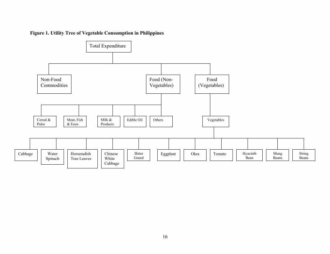
Figure 1 provides the utility trees of a representative household. Food consumption is

assumed to be indirectly separable from non-food consumption and vegetable consumption is

assumed to be indirectly separable from other food consumption. This procedure assumes that

the consumer’s utility maximization decision can be decomposed into three separate stages: in

the first stage, total expenditure is allocated over food and non-food items. In the second stage,

food expenditure is then allocated over vegetable and other food items. In the third stage,

vegetable expenditures are allocated over the following vegetable commodities: cabbage, water

spinach, horse radish tree leaves, Chinese white cabbage, bitter gourd, eggplant, okra, tomato,

hyacinth bean, mungbeans, string beans and other vegetables. These vegetable commodities were

3

chosen because they are the most commonly-used vegetables among all households in the

Philippines and they account for 78% of total vegetable expenditures.

< INSERT FIGURE 1 HERE >

We motivate our estimation in the context of multi-stage budgeting. Let q=[q1,q2,…qn]

denote the vector of goods demanded by the consumer and p= [p1,p2,…pn] be the corresponding

vector of all prices. Further, let y be the total expenditure and V(p) represent the indirect utility

function, which is continuous, nonincreasing and quasicovex in p, homogenous of degree zero in

(p,y). In general, by Roy’s identity, a household solves the following indirect utility function:

(1) Max 1 1 2 21 211 211 212 21 212 22 22( ( ), ( ( ( , , ... ), ), ( ))nV V p V V V p p p V V p .

Following Moschini (2001), the Marshallian unconditional demand functions qi(p) can be

expressed in terms of the first-stage and second-stage expenditure allocation function (y2(p),

y2i(p), and the third-stage conditional demand function ci(p21i), that is

(2) )(*)(

)(*)(

)(*

)()(

21

2

21

2

22

21 ii

i

ii

i

ipc

y

pypc

py

py

y

pypq == .

Equation (2) implies that the optimum within-group allocation is possible given only the group

price p21i, group expenditure allocation y2i, and total expenditure y.

At the same time, since the price P21i is unobservable, given expenditure y21i and

observable physical quantities q21i, most of analysis used the unit value Vi as representative of the

price P21i, which is calculated as

(3) i

i

iq

yV

21

21= .

However, as shown in Dong, Shonkwiler, and Capps (1998), Vi and y21i are endogenously

determined and can be expressed as:

(4) ),,(21 WyVfy ii = ,

4

where W is a vector of household characteristics. Therefore, the estimation of the quantity

demand system should be estimated simultaneously with the unit value system.

Moreover, since the total vegetable expenditure is endogenous with the share of

vegetable expenditure, a total vegetable expenditure equation related to total expenditure is

estimated based on a double-log relationship. The model to be estimated is as follows:

(5) i

kkik

ybsaay ε+×+∑+= )log()log(021

,

where the s’s are demographic and socioeconomic variables, the a’s and b’s are parameters to be

estimated, and i

ε is the usual disturbance term.

To estimate the demand system (2) for the Philippine vegetables considered in this

article, we adopt the Nonlinear Quadratic Almost Ideal Demand System (NQAIDS) developed

by Banks, Blundell and Lewbel (1997). Existing literature points to several advantages of the

NQAIDS over other flexible demand systems. In particular, these include nonlinearities and

interactions with household-specific characteristics in the utility effects (which are important for

household survey data) and better forecasting performance (Blundell, Pashardes, and Weber,

1993; Lyssiotou, Pashardes and Stengos, 2002). At the same time, this approach is amenable to

including demographic variables, which is important for this type of analysis due to the

individual household effects on vegetable consumption. The NQAIDS specification used in this

study can be represented as follows:

(6) 2

21 21 21 21

21

ln (ln ln ) ln(ln ln )j

ii i ij j ij i j i

j i j

j

w P Z y P y Pp

β

λα γ α β ε= + + + − + − +∑ ∑

∏,

where Z refer to demographic variables such as household size and educational achievement of

household head, P is the corresponding price index, w21i is the budget share of the ith vegetable,

5

iε is the error term, α's, β’s, and λ’s are parameters to be estimated. The price index P is defined

as:

(7) ∑∑+∑+=j i

jiijj

jjPPPP2121210

lnln2

1lnln γαα .

The symmetry, homogeneity and adding up constraints are imposed in the demand system

estimated.

2.2. Estimation Procedure

To deal with the potential endogeneity problem between the unit value equation (4), total

vegetable expenditure and the expenditure share equation (6), we adopt a three-step estimation

procedure. First, we estimate the parameters of the system of equations associated with unit

value equation (4) using seemingly unrelated regression (SUR). In the second step, an OLS

equation is used to predict total vegetable expenditure (y21i) based on total expenditure (y) (See

equation (5)). The third step involves using SUR to estimate the demand system in (6), using the

expected prices of the different vegetable commodities calculated in the first step and the total

predicted vegetable expenditure computed in the second step.

2.3 Elasticity Calculation

Following Pofahl, Capps, and Clauson (2005), the uncompensated own-price, and cross-

price elasticities associated with the NQAIDS are derived using the following expressions:

(8) ij

j

i

i

j

jij

j

ij

wpbp

wδκ

λβγα

γ−

+

+− ∑

2121

1)(

)(

2ln , where:

(8a) ∏=j

j

jppbβ

21)( ,

(8b) ∑∑−∑−−=j i

jiijj

jjjpppy

212121021lnln

2

1lnln γαακ , and

6

(8c) =

=otherwise

jiifij

1

0δ .

Expenditure elasticities are computed as:

(9)

++=

P

y

pbww i

i

i

i

i21

2121

log)(

21

λβε

Based on Slusky’s equation, the compensated price elasticities are derived:

(10) ji

U

ijij weee 21

** +=

where *

ije is the compensated price elasticity that corresponds to goods i and j , U

ije is the

uncompensated price elasticity of the same goods, and *

ie is the total expenditure elasticity of

good i.

3. Data and Empirical Results

3.1 Data

The data set used for the analysis is the 2003 Family Income and Expenditures Survey

(FIES) for the Philippines. These surveys were conducted every three years beginning in 1985

and the most recent of which was done in 2003. Note that only the 2003 data were made

available to us. The data set contains information on quantities and expenditures of over 50 food

items. As suggested in equation (3), the unit value or price is obtained from the ratio of its

associated expenditure to its associated quantity. For our purposes, we extracted the whole

vegetable section from the survey, which includes information for 39,264 households. Of these

households, 23,234 (59%) are classified as urban households and 16,030 (41%) are rural

households. The classification of households into urban or rural is based on the guidelines of the

Philippine Census of Population and Housing, where factors such as population density and

number of commercial establishments (among others) are considered.

7

As mentioned above, the following Philippine vegetable commodities were considered in

this study: cabbage, water spinach, horseradish tree leaves, Chinese white cabbage, bitter gourd,

eggplant, okra, tomato, hyacinth bean, mungbeans, string beans, and other vegetables. The total

food expenditures and the relevant quantities for each of the vegetables considered were also

extracted. Other demographic information for each household was also included in the data used

for estimation (i.e. household income, classification of urbanity, household size, age,

employment status, and presence of children).

The FIES survey adopts the “shuttle type” of data collection wherein respondents are

interviewed on two occasions using the same questionnaire. The 1st interview is usually done in

July of the reference year to gather data for the first 6 months of the year (January-June). The 2nd

interview is done in January of the following year, to account for the last 6 months (July –

December). The scheme is done to minimize memory bias and to capture the seasonality of

income and expenditure patterns. Annual data is estimated by combining the results of the 1st and

the 2nd visit. The concept of “average week” consumption for all food items was utilized.

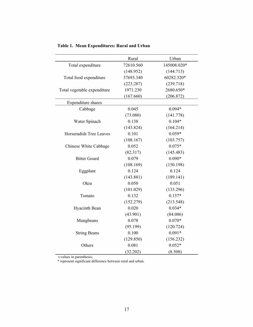
Just as a rough snapshot of the data, Table 1 provides a comparison of the mean

vegetable commodity expenditures between rural and urban households. Based on the average

vegetable expenditures, one may conclude that there is a significant difference between rural and

urban consumption behavior because expenditures in the urban areas tend to be twice as much as

in the rural areas. However, consumption behavior cannot be inferred simply from these mean

comparisons. A complete demand systems approach, which controls for a number of other

factors, would provide more credible information about the vegetable consumption behavior of

rural and urban households in the Philippines.

< INSERT TABLE 1 HERE >

8

3.2. Empirical Results

Using the three-step procedure described above, we first estimate the relevant demand

parameters of the demand system and then calculate the relevant elasticities of interest. However,

in the interest of space and in light of the large number of parameters estimated, the estimation

results are not presented here but are available from the authors upon request.

< INSERT TABLE 2 HERE >

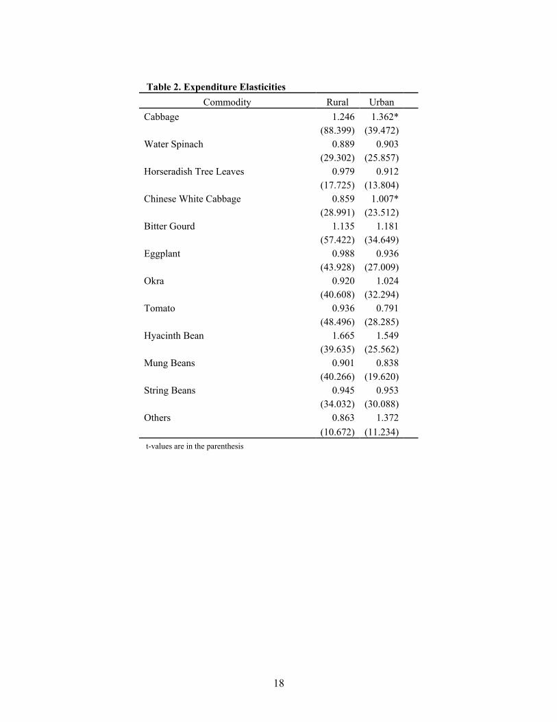
The expenditure elasticities for each of the Philippine vegetable commodities considered

are presented in Table 2. All expenditure elasticities are statistically significant at the 5% level.

In general, our estimated expenditure elasticities for the different vegetable commodities are

close to unitary values, which is consistent with previous studies (Quisumbing 1985; Belarmino

1983; Regalado 1985; Llanto 1998; Alba 1998). For both urban and rural areas, the commodities

of note are cabbage, bitter gourd, and hyacinth bean, which tend to have high expenditure

elasticities relative to the other vegetables. Larger expenditure elasticities for these three

commodities indicate that increasing income would induce more consumption of these

commodities relative to the other vegetables. This is especially true for cabbage which is

typically viewed as a luxury vegetable commodity in the Philippines since this vegetable crop is

typically commercially grown only in a handful of areas where the temperatures are low all year

round. This condition is atypical in a tropical country like the Philippines. At the other end of

the spectrum, tomato is another commodity of note since it tends to have lower expenditure

elasticity relative to the other vegetables (especially in the urban areas). This indicates that this

vegetable is viewed more as a necessity. Tomato as a necessity is not surprising as most simple

diets or viands in most areas in the Philippines use it as an ingredient to sauté fish, meat and

other vegetables (together with onions and garlic). Of the twelve vegetable commodities

9

considered, only cabbage and Chinese white cabbage have urban expenditure elasticities that are

significantly different from rural expenditure elasticities. Therefore, public policies that affect

income levels do not have a differential effect on vegetable consumption behavior in the rural

areas versus the urban areas (except for cabbage and Chinese white cabbage).

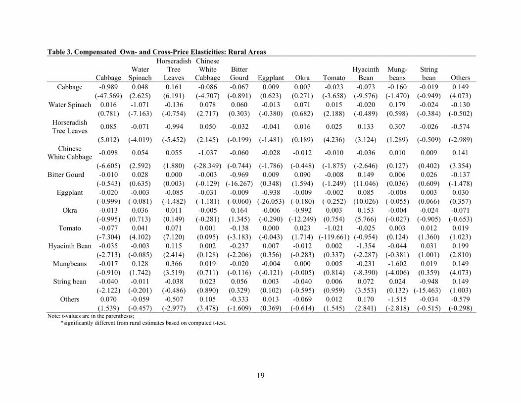
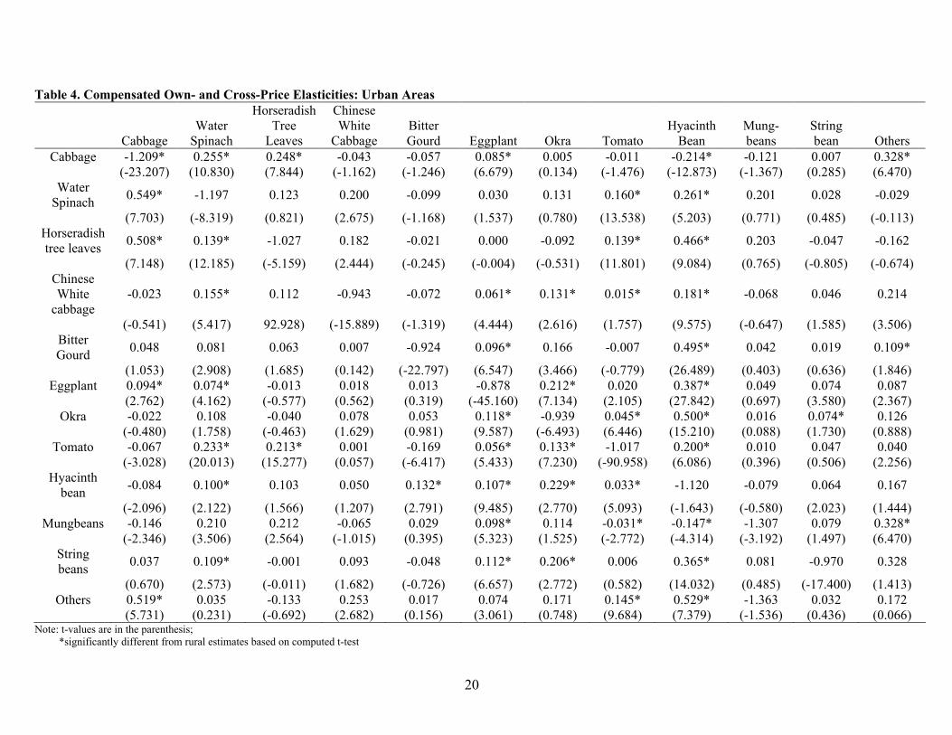
In Tables 3 and 4, estimates of compensated own- and cross-price elasticities for rural

and urban households are shown. The own-price elasticities are the values in the diagonal of the

tables. In the interest of conciseness the uncompensated elasticity estimates are not reported, but

are available from the authors upon request. Note that the results for the compensated and

uncompensated are very similar and the major behavioral patterns observed are the same.

< INSERT TABLES 3 AND 4 HERE >

The compensated own-price elasticities are statistically significant in both rural and urban

areas and carry the expected negative sign (Table 3). Our estimates also show that most rural

own-price elasticities are about unitary elastic, with the exception of hyacinth bean and

mungbeans whose demand are more elastic than the other vegetables (at -1.35 and -1.60,

respectively). The own-price elasticities of most vegetable commodities are larger in magnitude

for urban households relative to their rural counterparts (Table 4). More vegetables are own-

price elastic in the urban areas (relative to the urban areas): cabbage (-1.209), water spinach (-

1.197), hyacinth bean (-1.120), and mungbeans (-1.307). Also, note that the own-price

elasticities of most vegetables in the urban areas are not significantly different from the rural

own-price elasticity estimates (except for cabbage). This shows that vegetable consumption

response to price changes tend to be the same in the rural and urban areas. This is important

information for evaluating and implementing public policies that affect vegetable prices.

10

Tables 3 and 4 also shows there are a number of statistically significant cross-price

elasticities for the vegetables considered in the study. Positive cross-price elasticities indicate

substitutability, while negative cross-price elasticities indicate complementarity. Since it is

cumbersome to discuss the complementarity or substitutability of each possible pair of vegetable

commodity, we only discuss the general behavioral patterns observed from the cross-price

elasticity results. First, similar vegetable commodities that typically fall into the same vegetable

category tend to be substitutes. For example, most of the leafy vegetables (e.g. cabbage, water

spinach, horseradish tree leaves, and pechay) tend to be substitutes with the other leafy

vegetables. The “fruit” vegetables (e.g. bitter gourd, eggplant, okra, tomato, and hyacinth bean)

tend to be substitutes with other “fruit” vegetables. Second, across the broad vegetable

groupings, the particular vegetable commodities tend to be complements. For example, leafy

vegetables (i.e. cabbage) tend to be complements with tomato (i.e. fruit vegetables). The

complementarity observed across broad vegetable categories may be due to the nature of how

vegetables are cooked in the Philippines. That is, most of them are sautéed in oil or cooked

together with some mixture of sauce, seasoning, or soup base. The usual Philippine dishes with

vegetables always combine leafy and fruit vegetables, which supports the complementarity

across broad vegetable categories.

About a fifth of the own- and cross-price elasticity estimates are significantly different

between rural and urban households. These are indicated by asterisks in Table 4. In terms of

compensated own-price elasticities, only the price elasticity of cabbage differ in the urban areas

relative to the rural areas. In terms of the compensated cross-price elasticities, the differential

behavior of urban households (relative to rural households) are only observed in the degree of

responsiveness of most vegetable items to changes in cabbage, tomato, and hyacinth bean prices.

11

These results suggest that, on balance, the own-price and cross-price demand behavior of urban

households do not significantly differ from rural households.

Our results are consistent with Llanto (1998) in that for fruits and vegetables taken as a

group: (i) the dummy for urban areas proved insignificant; and (ii) demand was approximately

unitary price elastic for all households. On the other hand, our estimates are typically higher

than previous studies of vegetable demand (Quisumbing (1985); Belarmino (1983)), with own-

price elasticities for green, leafy and yellow vegetables that hover around -0.4 and -0.8. But note

that these studies use data that are about fifteen years prior to the one we use here. The

magnitude of demand responsiveness of Philippine consumers may have changed over time.

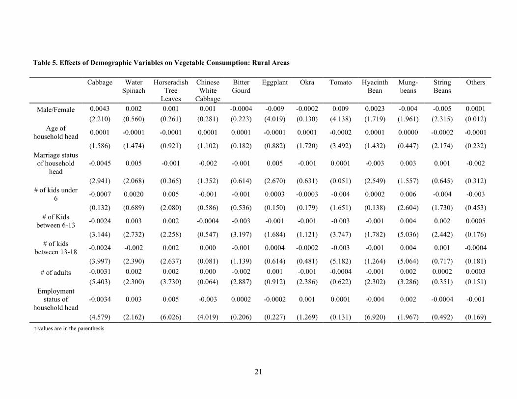
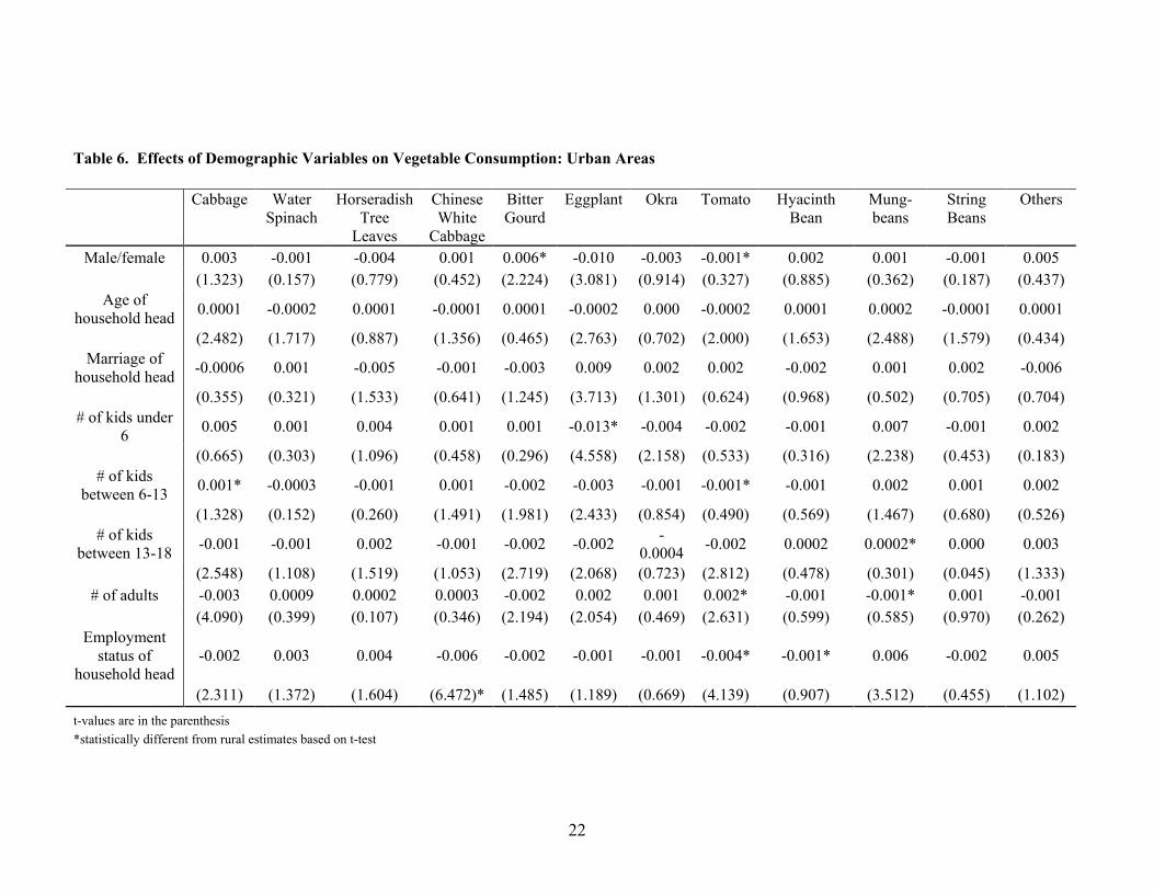
Tables 5 and 6 present the effect of a number of demographic variables on vegetable

demand for rural and urban households, respectively. In rural areas, marital status of the

household head significantly affects cabbage, water spinach, eggplant, and hyacinth bean

consumption. Age of the household head affects tomato and string beans consumption in the

rural areas. Gender of household head also affects cabbage, eggplant, tomato and string beans

demand in the rural areas. Lastly, the variables of family structure and employment status of

household head also significantly affect some of vegetable consumption in the rural areas. On the

other hand, marital status of the household head and gender does not have any significant effect

on any of the vegetable consumption in urban households. Comparing the demand impacts of the

various demographic variables in the rural and urban areas, only the effects of gender,

employment status of household head, and family structure variables tend to be significantly

different in the urban areas relative to the rural areas. On balance, for the majority of the

vegetable crops, there seems to be no significant difference between rural and urban households

in terms of the impact of changes in demographic variables on vegetable demand.

12

< INSERT TABLES 5 AND 6 HERE >

4. Conclusion and Policy Implications

This article compares vegetable demand behavior between rural and urban households in

the Philippines. A three-step methodology is used to solve endogeneity among the unit value,

total vegetable expenditure, and the expenditure share of different vegetables. An NQAIDS

approach is used to estimate the vegetable demand system primarily due to its flexibility and

accuracy (relative to other approaches in the literature).

For majority of the vegetable commodities examined, the expenditure, own-price, and

cross-price elasticities of urban households do not significantly differ from those of rural

households. The responsiveness of demand to demographic factors also typically do not differ

between rural and urban households. These results are indicative of a common vegetable demand

function for rural and urban households, at least for majority of the vegetable commodities.

However, note that there are still some vegetable commodities where demand behavior in the

urban areas significantly differs from the rural areas (i.e. cabbage).

The results from this study points to several policy implications. First, the general

observation that vegetable demand behavior tend to be the same for urban and rural households

indicates the possibility of simplified implementation of policies aimed to address nutritional

deficiencies in the Philippines. Instead of differential policy approaches in rural and urban areas,

an integrated approach may be more feasible. Second, the elasticity information generated from

this article would be useful for simulation and further analysis of various nutritional programs,

income stabilization policies, and food supply programs. In turn, these types of analyses would

enable quantification of the welfare effects of different policies and, consequently, aid in the

planning, design, and implementation of various government programs (i.e. agricultural price

13

stabilization schemes and poverty alleviation programs). Lastly, the elasticities calculated for the

different vegetable commodities can also be used to improve vegetable consumption forecasting

in the Philippines, an area in which empirical studies are nascent. Furthermore, the elasticities in

this study would be helpful in forecasting at the vegetable commodity level rather than at the

more aggregate levels. Information from these commodity level forecasts would be more useful

to policymakers and analysts.

14

References

Banks, J., R. Blundell and A. Lewbel (1997). “Quadratic Engel Curves and Consumer Demand.”

The Review of Economics and Statistics, 79, 527-539.

Belarmino, M. C. (1983). “Food Demand Matrix for Different Philippine Income Levels,”

Unpublished Ph.D. Dissertation, University of the Philippines at Los Banos.

Blundell, R., P. Pashardes and G. Weber. (1993). "What Do We Learn About Consumer Demand

Patterns from Micro Data?." American Economic Review, 83, 570-97.

Deaton, A. and J. Muellbauer (1980). Economics and Consumer Behavior. Cambridge

University Press.

Dong, D., J.S. Shonkwiler and O. Capps, Jr. (1998). “Estimation of Demand Functions Using

Cross-Sectional Household Data: The Problem Revisited.” American Journal of Agricultural

Economics, 80, 466-473.

Feng, X., and W. S. Chern (2000). “Demand for Healthy Food in the United States.” Selected

Paper at the American Agricultural Economics Association Annual Meeting, Tampa, Florida, 30

July – 2 August 2000.

FNRI (2004). http://www.fnri.dost.gov.ph/wp/dietlack.htm

Llanto, G. (1998). “Philippine Households’ Response to Price and Income Changes,” PIDS

Working Paper Series 98-02.

Lyssiotou, P., P. Pashardes and T. Stengos (2002). “Nesting Quadratic Logarithmic Demand

Systems,” Economics Letters, 76, 369-374.

Moschini, GianCarlo (2001). “A Flexible Multistage Demand System Based on Indirect

Separability,” Southern Economic Journal, 68, 22-41.

Orbeta, A. and M. Alba (1998). “Simulating the Impact of Macroeconomic Policy Changes on

the Nutrition Status of Households,” MIMAP Research Paper 21.

Pofahl, G., O. Capps, Jr. and A. Clauson (2005). “Demand for Non-Alcoholic Beverages:

Evidence from the ACNielsen Home Scan Panel.” Paper presented at the American Agricultural

Economics Association Annual Meeting, Providence, Rhode Island, 24-27 July 2005.

Quisumbing, A. (1985). Estimating the Distributional Impact of Food Market Intervention on

Policies on Nutrition, Unpublished Ph.D. Dissertation, University of the Philippines, School of

Economics.

15

Quisumbing, M. A., et al. (1988). “Flexible Function Form Estimates for Philippine Demand

Elasticities for Nutrition Simulation,” PIDS Working Paper Series 88-13.

Raper, K., M. Wanzala and R. Nayga, Jr. (2002). “Food Expenditures and Household

Demographic Composition in the U.S.: A Demand Systems Approach.” Applied Economics, 34,

981-992.

Regalado, B. M. (1985). The Distributional Impact of Food Policies in the Less-developed

Countries: The Case of the Philippines. Unpublished Master’s Thesis, University of the

Philippines at Los Banos.

San Juan, E. (1978). A Complete Demand Model for the Philippines. Unpublished Master’s

Thesis, University of the Philippines at Los Banos.

Schneeman B. (1997). Dietary Guidelines in Asian Countries Towards a Food-Based Appraoch.

Proceedings of a Seminar and Workshop on National Dietary Guidelines Meeting Nutritional

Needs of Asian Countries in the 21st Century. Singapore, 27-28 July 1997.

Wan, G. (1996). “Income Elasticities of Household Demand in Rural China: Estimates from

Cross-Sectional Survey Data.” Journal of Economic Studies, 23, 18-33.

16

Figure 1. Utility Tree of Vegetable Consumption in Philippines

Total Expenditure

Non-Food

Commodities

Food (Non-

Vegetables)

Cereal &

Pulse

Meat, Fish

& Eggs

Milk &

Products Others Vegetables

Hyacinth

Bean Tomato Okra Eggplant Bitter

Gourd

Food

(Vegetables)

Chinese

White

Cabbage

Horseradish

Tree Leaves

Water

Spinach

Cabbage Mung

Beans

Edible Oil

String

Beans

17

Table 1. Mean Expenditures: Rural and Urban

Rural Urban

Total expenditure 72610.560 145008.020*

(148.952) (144.713)

Total food expenditure 37693.340 60282.320*

(223.287) (239.718)

Total vegetable expenditure 1971.230 2680.650*

(167.660) (206.872)

Expenditure shares

Cabbage 0.045 0.094*

(73.080) (141.778)

Water Spinach 0.138 0.104*

(143.824) (164.214)

Horseradish Tree Leaves 0.101 0.059*

(108.167) (103.757)

Chinese White Cabbage 0.052 0.075*

(82.317) (145.483)

Bitter Gourd 0.079 0.090*

(108.169) (150.198)

Eggplant 0.124 0.124

(143.881) (189.141)

Okra 0.050 0.051

(101.029) (133.296)

Tomato 0.132 0.157*

(152.279) (213.548)

Hyacinth Bean 0.020 0.034*

(43.901) (84.086)

Mungbeans 0.078 0.070*

(95.199) (120.724)

String Beans 0.100 0.091*

(129.850) (156.232)

Others 0.081 0.052*

(32.202) (8.508) t-values in parenthesis;

* represent significant difference between rural and urban.

18

Table 2. Expenditure Elasticities

Commodity Rural Urban

Cabbage 1.246 1.362*

(88.399) (39.472)

Water Spinach 0.889 0.903

(29.302) (25.857)

Horseradish Tree Leaves 0.979 0.912

(17.725) (13.804)

Chinese White Cabbage 0.859 1.007*

(28.991) (23.512)

Bitter Gourd 1.135 1.181

(57.422) (34.649)

Eggplant 0.988 0.936

(43.928) (27.009)

Okra 0.920 1.024

(40.608) (32.294)

Tomato 0.936 0.791

(48.496) (28.285)

Hyacinth Bean 1.665 1.549

(39.635) (25.562)

Mung Beans 0.901 0.838

(40.266) (19.620)

String Beans 0.945 0.953

(34.032) (30.088)

Others 0.863 1.372

(10.672) (11.234)

t-values are in the parenthesis

19

Table 3. Compensated Own- and Cross-Price Elasticities: Rural Areas

Cabbage

Water

Spinach

Horseradish

Tree

Leaves

Chinese

White

Cabbage

Bitter

Gourd Eggplant Okra Tomato

Hyacinth

Bean

Mung-

beans

String

bean Others

Cabbage -0.989 0.048 0.161 -0.086 -0.067 0.009 0.007 -0.023 -0.073 -0.160 -0.019 0.149

(-47.569) (2.625) (6.191) (-4.707) (-0.891) (0.623) (0.271) (-3.658) (-9.576) (-1.470) (-0.949) (4.073)

Water Spinach 0.016 -1.071 -0.136 0.078 0.060 -0.013 0.071 0.015 -0.020 0.179 -0.024 -0.130

(0.781) (-7.163) (-0.754) (2.717) (0.303) (-0.380) (0.682) (2.188) (-0.489) (0.598) (-0.384) (-0.502)

Horseradish

Tree Leaves 0.085 -0.071 -0.994 0.050 -0.032 -0.041 0.016 0.025 0.133 0.307 -0.026 -0.574

(5.012) (-4.019) (-5.452) (2.145) (-0.199) (-1.481) (0.189) (4.236) (3.124) (1.289) (-0.509) (-2.989)

Chinese

White Cabbage -0.098 0.054 0.055 -1.037 -0.060 -0.028 -0.012 -0.010 -0.036 0.010 0.009 0.141

(-6.605) (2.592) (1.880) (-28.349) (-0.744) (-1.786) (-0.448) (-1.875) (-2.646) (0.127) (0.402) (3.354)

Bitter Gourd -0.010 0.028 0.000 -0.003 -0.969 0.009 0.090 -0.008 0.149 0.006 0.026 -0.137

(-0.543) (0.635) (0.003) (-0.129) (-16.267) (0.348) (1.594) (-1.249) (11.046) (0.036) (0.609) (-1.478)

Eggplant -0.020 -0.003 -0.085 -0.031 -0.009 -0.938 -0.009 -0.002 0.085 -0.008 0.003 0.030

(-0.999) (-0.081) (-1.482) (-1.181) (-0.060) (-26.053) (-0.180) (-0.252) (10.026) (-0.055) (0.066) (0.357)

Okra -0.013 0.036 0.011 -0.005 0.164 -0.006 -0.992 0.003 0.153 -0.004 -0.024 -0.071

(-0.995) (0.713) (0.149) (-0.281) (1.345) (-0.290) (-12.249) (0.754) (5.766) (-0.027) (-0.905) (-0.653)

Tomato -0.077 0.041 0.071 0.001 -0.138 0.000 0.023 -1.021 -0.025 0.003 0.012 0.019

(-7.304) (4.102) (7.120) (0.095) (-3.183) (-0.043) (1.714) (-119.661) (-0.954) (0.124) (1.360) (1.023)

Hyacinth Bean -0.035 -0.003 0.115 0.002 -0.237 0.007 -0.012 0.002 -1.354 -0.044 0.031 0.199

(-2.713) (-0.085) (2.414) (0.128) (-2.206) (0.356) (-0.283) (0.337) (-2.287) (-0.381) (1.001) (2.810)

Mungbeans -0.017 0.128 0.366 0.019 -0.020 -0.004 0.000 0.005 -0.231 -1.602 0.019 0.149

(-0.910) (1.742) (3.519) (0.711) (-0.116) (-0.121) (-0.005) (0.814) (-8.390) (-4.006) (0.359) (4.073)

String bean -0.040 -0.011 -0.038 0.023 0.056 0.003 -0.040 0.006 0.072 0.024 -0.948 0.149

(-2.122) (-0.201) (-0.486) (0.890) (0.329) (0.102) (-0.595) (0.959) (3.553) (0.132) (-15.463) (1.003)

Others 0.070 -0.059 -0.507 0.105 -0.333 0.013 -0.069 0.012 0.170 -1.515 -0.034 -0.579

(1.539) (-0.457) (-2.977) (3.478) (-1.609) (0.369) (-0.614) (1.545) (2.841) (-2.818) (-0.515) (-0.298) Note: t-values are in the parenthesis;

*significantly different from rural estimates based on computed t-test.

20

Table 4. Compensated Own- and Cross-Price Elasticities: Urban Areas

Cabbage

Water

Spinach

Horseradish

Tree

Leaves

Chinese

White

Cabbage

Bitter

Gourd Eggplant Okra Tomato

Hyacinth

Bean

Mung-

beans

String

bean Others

Cabbage -1.209* 0.255* 0.248* -0.043 -0.057 0.085* 0.005 -0.011 -0.214* -0.121 0.007 0.328*

(-23.207) (10.830) (7.844) (-1.162) (-1.246) (6.679) (0.134) (-1.476) (-12.873) (-1.367) (0.285) (6.470)

Water

Spinach 0.549* -1.197 0.123 0.200 -0.099 0.030 0.131 0.160* 0.261* 0.201 0.028 -0.029

(7.703) (-8.319) (0.821) (2.675) (-1.168) (1.537) (0.780) (13.538) (5.203) (0.771) (0.485) (-0.113)

Horseradish

tree leaves 0.508* 0.139* -1.027 0.182 -0.021 0.000 -0.092 0.139* 0.466* 0.203 -0.047 -0.162

(7.148) (12.185) (-5.159) (2.444) (-0.245) (-0.004) (-0.531) (11.801) (9.084) (0.765) (-0.805) (-0.674)

Chinese

White

cabbage

-0.023 0.155* 0.112 -0.943 -0.072 0.061* 0.131* 0.015* 0.181* -0.068 0.046 0.214

(-0.541) (5.417) 92.928) (-15.889) (-1.319) (4.444) (2.616) (1.757) (9.575) (-0.647) (1.585) (3.506)

Bitter

Gourd 0.048 0.081 0.063 0.007 -0.924 0.096* 0.166 -0.007 0.495* 0.042 0.019 0.109*

(1.053) (2.908) (1.685) (0.142) (-22.797) (6.547) (3.466) (-0.779) (26.489) (0.403) (0.636) (1.846)

Eggplant 0.094* 0.074* -0.013 0.018 0.013 -0.878 0.212* 0.020 0.387* 0.049 0.074 0.087

(2.762) (4.162) (-0.577) (0.562) (0.319) (-45.160) (7.134) (2.105) (27.842) (0.697) (3.580) (2.367)

Okra -0.022 0.108 -0.040 0.078 0.053 0.118* -0.939 0.045* 0.500* 0.016 0.074* 0.126

(-0.480) (1.758) (-0.463) (1.629) (0.981) (9.587) (-6.493) (6.446) (15.210) (0.088) (1.730) (0.888)

Tomato -0.067 0.233* 0.213* 0.001 -0.169 0.056* 0.133* -1.017 0.200* 0.010 0.047 0.040

(-3.028) (20.013) (15.277) (0.057) (-6.417) (5.433) (7.230) (-90.958) (6.086) (0.396) (0.506) (2.256)

Hyacinth

bean -0.084 0.100* 0.103 0.050 0.132* 0.107* 0.229* 0.033* -1.120 -0.079 0.064 0.167

(-2.096) (2.122) (1.566) (1.207) (2.791) (9.485) (2.770) (5.093) (-1.643) (-0.580) (2.023) (1.444)

Mungbeans -0.146 0.210 0.212 -0.065 0.029 0.098* 0.114 -0.031* -0.147* -1.307 0.079 0.328*

(-2.346) (3.506) (2.564) (-1.015) (0.395) (5.323) (1.525) (-2.772) (-4.314) (-3.192) (1.497) (6.470)

String

beans 0.037 0.109* -0.001 0.093 -0.048 0.112* 0.206* 0.006 0.365* 0.081 -0.970 0.328

(0.670) (2.573) (-0.011) (1.682) (-0.726) (6.657) (2.772) (0.582) (14.032) (0.485) (-17.400) (1.413)

Others 0.519* 0.035 -0.133 0.253 0.017 0.074 0.171 0.145* 0.529* -1.363 0.032 0.172

(5.731) (0.231) (-0.692) (2.682) (0.156) (3.061) (0.748) (9.684) (7.379) (-1.536) (0.436) (0.066) Note: t-values are in the parenthesis;

*significantly different from rural estimates based on computed t-test

21

Table 5. Effects of Demographic Variables on Vegetable Consumption: Rural Areas

Cabbage Water

Spinach

Horseradish

Tree

Leaves

Chinese

White

Cabbage

Bitter

Gourd

Eggplant Okra Tomato Hyacinth

Bean

Mung-

beans

String

Beans

Others

Male/Female 0.0043 0.002 0.001 0.001 -0.0004 -0.009 -0.0002 0.009 0.0023 -0.004 -0.005 0.0001

(2.210) (0.560) (0.261) (0.281) (0.223) (4.019) (0.130) (4.138) (1.719) (1.961) (2.315) (0.012)

Age of

household head 0.0001 -0.0001 -0.0001 0.0001 0.0001 -0.0001 0.0001 -0.0002 0.0001 0.0000 -0.0002 -0.0001

(1.586) (1.474) (0.921) (1.102) (0.182) (0.882) (1.720) (3.492) (1.432) (0.447) (2.174) (0.232)

Marriage status

of household

head

-0.0045 0.005 -0.001 -0.002 -0.001 0.005 -0.001 0.0001 -0.003 0.003 0.001 -0.002

(2.941) (2.068) (0.365) (1.352) (0.614) (2.670) (0.631) (0.051) (2.549) (1.557) (0.645) (0.312)

# of kids under

6 -0.0007 0.0020 0.005 -0.001 -0.001 0.0003 -0.0003 -0.004 0.0002 0.006 -0.004 -0.003

(0.132) (0.689) (2.080) (0.586) (0.536) (0.150) (0.179) (1.651) (0.138) (2.604) (1.730) (0.453)

# of Kids

between 6-13 -0.0024 0.003 0.002 -0.0004 -0.003 -0.001 -0.001 -0.003 -0.001 0.004 0.002 0.0005

(3.144) (2.732) (2.258) (0.547) (3.197) (1.684) (1.121) (3.747) (1.782) (5.036) (2.442) (0.176)

# of kids

between 13-18 -0.0024 -0.002 0.002 0.000 -0.001 0.0004 -0.0002 -0.003 -0.001 0.004 0.001 -0.0004

(3.997) (2.390) (2.637) (0.081) (1.139) (0.614) (0.481) (5.182) (1.264) (5.064) (0.717) (0.181)

# of adults -0.0031 0.002 0.002 0.000 -0.002 0.001 -0.001 -0.0004 -0.001 0.002 0.0002 0.0003

(5.403) (2.300) (3.730) (0.064) (2.887) (0.912) (2.386) (0.622) (2.302) (3.286) (0.351) (0.151)

Employment

status of

household head

-0.0034 0.003 0.005 -0.003 0.0002 -0.0002 0.001 0.0001 -0.004 0.002 -0.0004 -0.001

(4.579) (2.162) (6.026) (4.019) (0.206) (0.227) (1.269) (0.131) (6.920) (1.967) (0.492) (0.169)


22

Table 6. Effects of Demographic Variables on Vegetable Consumption: Urban Areas

Cabbage Water

Spinach

Horseradish

Tree

Leaves

Chinese

White

Cabbage

Bitter

Gourd

Eggplant Okra Tomato Hyacinth

Bean

Mung-

beans

String

Beans

Others

Male/female 0.003 -0.001 -0.004 0.001 0.006* -0.010 -0.003 -0.001* 0.002 0.001 -0.001 0.005

(1.323) (0.157) (0.779) (0.452) (2.224) (3.081) (0.914) (0.327) (0.885) (0.362) (0.187) (0.437)

Age of

household head 0.0001 -0.0002 0.0001 -0.0001 0.0001 -0.0002 0.000 -0.0002 0.0001 0.0002 -0.0001 0.0001

(2.482) (1.717) (0.887) (1.356) (0.465) (2.763) (0.702) (2.000) (1.653) (2.488) (1.579) (0.434)

Marriage of

household head -0.0006 0.001 -0.005 -0.001 -0.003 0.009 0.002 0.002 -0.002 0.001 0.002 -0.006

(0.355) (0.321) (1.533) (0.641) (1.245) (3.713) (1.301) (0.624) (0.968) (0.502) (0.705) (0.704)

# of kids under

6 0.005 0.001 0.004 0.001 0.001 -0.013* -0.004 -0.002 -0.001 0.007 -0.001 0.002

(0.665) (0.303) (1.096) (0.458) (0.296) (4.558) (2.158) (0.533) (0.316) (2.238) (0.453) (0.183)

# of kids

between 6-13 0.001* -0.0003 -0.001 0.001 -0.002 -0.003 -0.001 -0.001* -0.001 0.002 0.001 0.002

(1.328) (0.152) (0.260) (1.491) (1.981) (2.433) (0.854) (0.490) (0.569) (1.467) (0.680) (0.526)

# of kids

between 13-18 -0.001 -0.001 0.002 -0.001 -0.002 -0.002

-

0.0004 -0.002 0.0002 0.0002* 0.000 0.003

(2.548) (1.108) (1.519) (1.053) (2.719) (2.068) (0.723) (2.812) (0.478) (0.301) (0.045) (1.333)

# of adults -0.003 0.0009 0.0002 0.0003 -0.002 0.002 0.001 0.002* -0.001 -0.001* 0.001 -0.001

(4.090) (0.399) (0.107) (0.346) (2.194) (2.054) (0.469) (2.631) (0.599) (0.585) (0.970) (0.262)

Employment

status of

household head

-0.002 0.003 0.004 -0.006 -0.002 -0.001 -0.001 -0.004* -0.001* 0.006 -0.002 0.005

(2.311) (1.372) (1.604) (6.472)* (1.485) (1.189) (0.669) (4.139) (0.907) (3.512) (0.455) (1.102)


*statistically different from rural estimates based on t-test

Documents

Household Vegetable Demand in the Philippines - AgEcon