Embed Size (px)
Citation preview
Distributed Vision with Smart Pixels
Sándor P. FeketeAlgorithms Group
Braunschweig Institute ofTechnologyGermany
Dietmar FeyInstitute for Computer Science
Friedrich-Schiller-UniversityJena, Germany
Marcus KomannInstitute for Computer Science
Friedrich-Schiller-UniversityJena, Germany
Alexander KröllerAlgorithms Group
Braunschweig Institute ofTechnologyGermany
Marc ReichenbachInstitute for Computer Science
Friedrich-Schiller-UniversityJena, Germany
Christiane SchmidtAlgorithms Group
Braunschweig Institute ofTechnologyGermany
ABSTRACTWe study a problem related to computer vision: How can afield of sensors compute higher-level properties of observedobjects deterministically in sublinear time, without access-ing a central authority? This issue is not only important forreal-time processing of images, but lies at the very heart ofunderstanding how a brain may be able to function.
In particular, we consider a quadratic field of n ”smartpixels” on a video chip that observe a B/W image. Eachpixel can exchange low-level information with its immedi-ate neighbors. We show that it is possible to compute thecenters of gravity along with a principal component analysisof all connected components of the black grid graph in timeO(√n), by developing appropriate distributed protocols that
are modeled after sweepline methods.Our method is not only interesting from a philosophical
and theoretical point of view, it is also useful for actual ap-plications for controling a robot arm that has to seize objectson a moving belt. We describe details of an implementationon an FPGA; the code has also been turned into a hardwaredesign for an application-specific integrated circuit (ASIC).
Categories and Subject DescriptorsF.2.2 [Analysis of Algorithms and Problem Complex-ity]: Nonnumerical Algorithms and Problems (E.2-5, G.2,H.2-3)—Geometrical problems and computations
General TermsAlgorithms
Permission to make digital or hard copies of all or part of this work forpersonal or classroom use is granted without fee provided that copies arenot made or distributed for profit or commercial advantage and that copiesbear this notice and the full citation on the first page. To copy otherwise, torepublish, to post on servers or to redistribute to lists, requires prior specificpermission and/or a fee.SCG’09, June 8–10, 2009, Aarhus, Denmark.Copyright 2009 ACM 978-1-60558-501-7/09/06 ...$5.00.
Keywordsdistributed vision, distributed algorithms, sublinear algo-rithms, principal component analysis, sweepline algorithms.
1. INTRODUCTIONFast Geometric Algorithms. A major part of the
research conducted in computational geometry shoots formuch more than just polynomial runtime. Often motivatedby applications from areas such as computer graphics orcomputer vision, some of the most impressive work has re-sulted in linear-time methods, e.g., for triangulating a sim-ple polygon [6]. However, speed and accuracy of geomet-ric processing may not just matter in terms of theoreticalCPU time; it can also make the difference between efficientquality control for ready-made food [20] or letting defectiveproducts leave the factory; between a robot arm accuratelyseizing a large variety of machine parts from a conveyor beltor production coming to a sudden and unplanned, screech-ing halt [5]; between a baseball player cleanly catching a linedrive or being hit squarely into the face [12].
Vision. Throughout human evolution, quality and speedof visual processing has not only been a matter of win or loss,but of life and death. As a result, human vision is not justbased on amazing software for image processing, but also onextremely powerful hardware. How does the human brainprocess visual information and what can we learn from it?This has been one of the most intriguing scientific questionsever, not just in computer science, but also neurobiology, art,and philosophy [16]. Quite clearly, human vision consistsof different mechanisms and filters, combining a variety offast heuristics, parallel algorithms, but also sophisticatedalgorithms for performing highly specialized analytic tasks.
Processing Visual Information. How do computersprocess visual information? Typically, the input from a gridof pixels is fed into the CPU, where more or less sophisti-cated operations are performed. Quite clearly, just lookingat the input takes least linear time for whatever problemis to be solved in a deterministic manner. Can we learnanything about or from the functioning of our brain? Whendiscussing human vision, even the innocent expression“look-ing at the input” alludes to a philosophical issue that goesmuch deeper when trying to understand image processing
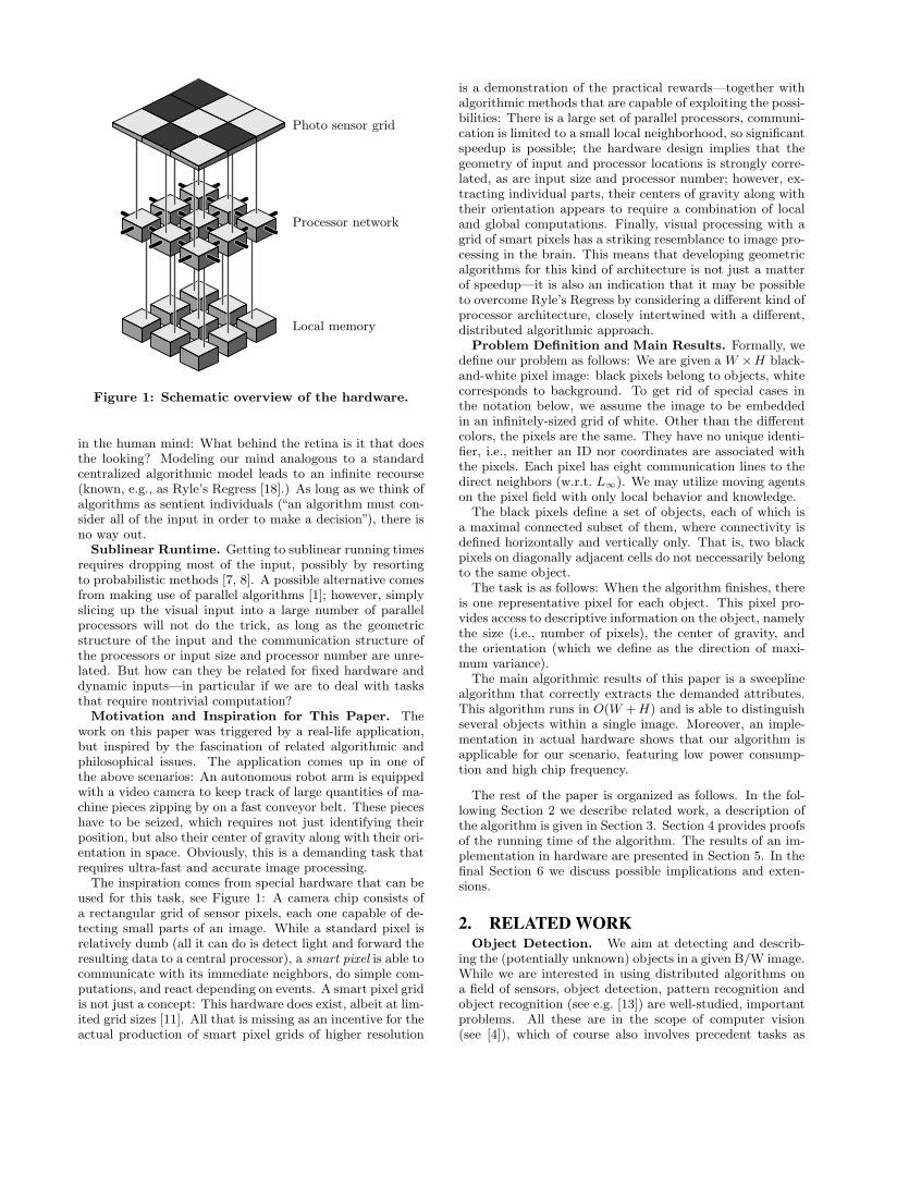
Local memory
Processor network
Photo sensor grid
Figure 1: Schematic overview of the hardware.
in the human mind: What behind the retina is it that doesthe looking? Modeling our mind analogous to a standardcentralized algorithmic model leads to an infinite recourse(known, e.g., as Ryle’s Regress [18].) As long as we think ofalgorithms as sentient individuals (“an algorithm must con-sider all of the input in order to make a decision”), there isno way out.
Sublinear Runtime. Getting to sublinear running timesrequires dropping most of the input, possibly by resortingto probabilistic methods [7, 8]. A possible alternative comesfrom making use of parallel algorithms [1]; however, simplyslicing up the visual input into a large number of parallelprocessors will not do the trick, as long as the geometricstructure of the input and the communication structure ofthe processors or input size and processor number are unre-lated. But how can they be related for fixed hardware anddynamic inputs—in particular if we are to deal with tasksthat require nontrivial computation?
Motivation and Inspiration for This Paper. Thework on this paper was triggered by a real-life application,but inspired by the fascination of related algorithmic andphilosophical issues. The application comes up in one ofthe above scenarios: An autonomous robot arm is equippedwith a video camera to keep track of large quantities of ma-chine pieces zipping by on a fast conveyor belt. These pieceshave to be seized, which requires not just identifying theirposition, but also their center of gravity along with their ori-entation in space. Obviously, this is a demanding task thatrequires ultra-fast and accurate image processing.
The inspiration comes from special hardware that can beused for this task, see Figure 1: A camera chip consists ofa rectangular grid of sensor pixels, each one capable of de-tecting small parts of an image. While a standard pixel isrelatively dumb (all it can do is detect light and forward theresulting data to a central processor), a smart pixel is able tocommunicate with its immediate neighbors, do simple com-putations, and react depending on events. A smart pixel gridis not just a concept: This hardware does exist, albeit at lim-ited grid sizes [11]. All that is missing as an incentive for theactual production of smart pixel grids of higher resolution
is a demonstration of the practical rewards—together withalgorithmic methods that are capable of exploiting the possi-bilities: There is a large set of parallel processors, communi-cation is limited to a small local neighborhood, so significantspeedup is possible; the hardware design implies that thegeometry of input and processor locations is strongly corre-lated, as are input size and processor number; however, ex-tracting individual parts, their centers of gravity along withtheir orientation appears to require a combination of localand global computations. Finally, visual processing with agrid of smart pixels has a striking resemblance to image pro-cessing in the brain. This means that developing geometricalgorithms for this kind of architecture is not just a matterof speedup—it is also an indication that it may be possibleto overcome Ryle’s Regress by considering a different kind ofprocessor architecture, closely intertwined with a different,distributed algorithmic approach.
Problem Definition and Main Results. Formally, wedefine our problem as follows: We are given a W ×H black-and-white pixel image: black pixels belong to objects, whitecorresponds to background. To get rid of special cases inthe notation below, we assume the image to be embeddedin an infinitely-sized grid of white. Other than the differentcolors, the pixels are the same. They have no unique identi-fier, i.e., neither an ID nor coordinates are associated withthe pixels. Each pixel has eight communication lines to thedirect neighbors (w.r.t. L∞). We may utilize moving agentson the pixel field with only local behavior and knowledge.
The black pixels define a set of objects, each of which isa maximal connected subset of them, where connectivity isdefined horizontally and vertically only. That is, two blackpixels on diagonally adjacent cells do not neccessarily belongto the same object.
The task is as follows: When the algorithm finishes, thereis one representative pixel for each object. This pixel pro-vides access to descriptive information on the object, namelythe size (i.e., number of pixels), the center of gravity, andthe orientation (which we define as the direction of maxi-mum variance).
The main algorithmic results of this paper is a sweeplinealgorithm that correctly extracts the demanded attributes.This algorithm runs in O(W +H) and is able to distinguishseveral objects within a single image. Moreover, an imple-mentation in actual hardware shows that our algorithm isapplicable for our scenario, featuring low power consump-tion and high chip frequency.
The rest of the paper is organized as follows. In the fol-lowing Section 2 we describe related work, a description ofthe algorithm is given in Section 3. Section 4 provides proofsof the running time of the algorithm. The results of an im-plementation in hardware are presented in Section 5. In thefinal Section 6 we discuss possible implications and exten-sions.
2. RELATED WORKObject Detection. We aim at detecting and describ-
ing the (potentially unknown) objects in a given B/W image.While we are interested in using distributed algorithms ona field of sensors, object detection, pattern recognition andobject recognition (see e.g. [13]) are well-studied, importantproblems. All these are in the scope of computer vision(see [4]), which of course also involves precedent tasks as
describing an image, on this basis recognition—recognizinglocal discontinuities in intensity for identifying edges and,more sophisticated, segments, shape and clusters. Object,pattern or face recognition concentrates on certifying whetherpre-defined or learned objects (patterns, faces) or objectclasses are present in the given image. Object identifica-tion deals with an even more specified task: within a givenclass (e.g., cars) a certain object is to be identified, see [10].By contrast, we want to detect an unknown object (or ob-jects) and determine, e.g., its center of gravity. While thetask of distinguishing the object from the background is—aswe face monochrome images—not our focus of interest.
Principal Component Analysis. For the detectedobjects we are interested in several attributes, like centroidposition or orientation. These attributes can be describedby moments. For given data sets, attributes like orientationcan be determined with a Principal Component Analysis(PCA) [14, 19]. This analysis is widely used for statisti-cal analysis of data, e.g., from neuroscience, gene expressiondata (see [21]), as well as in computer vision, for both rep-resentation (see [13]) and image compression.
Determining the eigenvectors of the covariance matrix andordering these by the related eigenvalue (highest to lowest),gives the components in order of significance. That is, for vi-sualized data with coordinates the first principal componentgives the orientation.
Distributed Algorithms. Our main contribution inthis paper is a distributed sweep over the objects. A straight-forward approach would be to run standard distributed algo-rithm on the graph induced by the object pixels. Any leaderelection or spanning tree algorithm could be used instead ofour algorithm, see [2, 3, 9]. A distributed algorithm thatstays within the object pixels can not have a better runtimethan Ω(m2) for objects on an m×m-pixel image, as there areobjects with such a graph diameter. Our algorithm fully ex-ploits the geometric structure of the underlying network byalso running on non-object pixels, resulting in a distributedtime complexity of O(m).
Own work. We published a predecessor paper [15] tothis one. It contains the same distributed mechanism tocompute the desired values as in this paper, so we keep theaccording Section 3.1 informal here. The mentioned paperdoes not contain the distributed sweep algorithm, which isthe major contribution here. Instead, we described a heuris-tic that works reasonably well on convex and well-separatedobjects, yet did not allow us to prove any quality measures.
3. THE ALGORITHMIn this section we describe the problem settings as well as
the parts of our algorithm.Pixel Grid. We assume there is an infinite grid of smart
pixels. All pixels are completely identical, that is, they haveneither a unique ID, nor coordinates available. This assump-tion is helpful for our application, as it allows us to reset thegrid to a clean initial state between runs, i.e., without havingto run a global initialization algorithm.
Each pixel p can communicate with its 8 direct neighbors,this set is denoted by Γ(p). We define Γ(p) := Γ(p) ∪ p.The pixels in Γ(p) are identified by direction and denotedN(p), NW(p), W(p), SW(p), S(p), SE(p), E(p), and NE(p),with the obvious interpretation.
Distributed Model. We use the synchronized LOCALmodel by Peleg [17]. To be precise, our pixel network runs in
synchronized rounds. In each round, each pixel may performany computation on the data it has available, and it maysend any amount of data to its neighbors.
Objects. There is a photo X overlayed on the pixel grid.Each pixel p either sees part of the objects (if p ∈ X ), orit sees the background. In the first communication round,the pixels exchange this information with their neighbors.In the algorithm below, we assume each pixel p to knowthe object status of all pixels in Γ(p). X may consist ofmultiple objects. We say that two pixels in X belong tothe same object, if they can be connected by a path in Xusing only horizontal and vertical steps (that is, an object isa connected component of X in the canonical 4-regular gridgraph).
3.1 MomentsWe already described our scheme for calculating the mo-
ments (without the sweep algorithm) in a previous paper [15].Here we just summarize it, so that the reader can get a com-plete picture of the algorithm.
Let X ′ ⊆ X be an object in X . Our aim is to calculate
1. The size |X ′| of the object.
2. The center of gravity (µx, µy) of the object, i.e.,
µx =1
|X ′|X
p∈X ′
xp , µy =1
|X ′|X
p∈X ′
yp , (1)
where (xp, yp) are the coordinates of pixel p in someglobal coordinate system.
3. The second moments in the form of the covariance ma-trix „
σ2x σxy
σxy σ2y
«, (2)
where we see the object as a point distribution on R2.The two Principal Component Axes are then definedby the Eigenvectors of this matrix, see [19]. The appli-cation uses them to identify the direction of greatestvariance, which is used as the orientation (rotation) ofthe object on the belt.
As the pixels do not know the global coordinate system, wecannot compute these values directly. Instead, we employ amechanism of cumulating relative weights. We construct ascheme by which agents sweep over the object. The agents“consume” the “weight” of object pixels as they pass, andthey eventually collect these picked up weights in a singlepixel. Each object pixel has a weight of 1, and this weightcan only be consumed once.
Each agent on a pixel (x, y), and possessing the weightsfor object pixels X ⊆ X ′ carries the following six-tuple:
(|X|,Xp∈X
(x− xp),Xp∈X
(y − yp),Xp∈X
(x− xp)2,
Xp∈X
(y − yp)2,Xp∈X
(x− xp)(y − yp)).(3)
This tuple has a number of nice properties. These are easy toconfirm, a full description with proofs can be found in [15]:
• These values are sufficient to compute the aforemen-tioned moments, if (x, y) is known. We assume that
after our algorithm finished, a centralized processorwill pick up the tuple from the single pixel per object,compute the moments, and uses them for whatever ac-tivity the machine was built.
• When an agent moves from (x, y) to an adjacent pixel,it is computationally trivial to update the tuple forthe new position. For example, when moving a tuple(m, sx, sy, sxx, syy, sxy) to the east, (m, sx−m, sy, sxx−2sx +m, syy, sxy − sy) is the correct tuple for the newposition. Addition and subtraction are sufficient forall necessary updates.
• If an agent picks up the weight of the pixel it currentlyresides on, it simply has to increment the first tupleentry.
• If an agent receives the cumulative weight of anotheragent on the same pixel, it just computes the component-wise sum of the two tuples.
So all that is left to do is to define a rule set by which agentscan sweep over the objects, pick up the weights, and let theweights for each object cumulate in a single pixel. This iswhat we describe next.
3.2 AgentsLet A denote the set of all agents. An agent a ∈ A has
the following variables in addition to those for calculatingmoments:
• Ca ⊆ A, a set of partners. Partners are agents thatbelong to the same object, living in an adjacent row.Once agents decide to partner, they move together andstay within a horizontal distance of at most 1. Ini-tially, Ca = ∅. Partnership will be mutual throughoutthe algorithm, so one can think of partnership as anundirected graph on the set of agents. This graph isdenoted by C = (A,C).
• ha, a boolean stating whether the agent has ever leftthe object it started in. The variable is initialized asfalse (as agents are always created on object pixels).When the agent moves onto a non-object pixel, it setsha ← true.
We denote the set of all agents that are currently on a pixelp by A(p) ⊆ A. We assume that each agent has access tothe following information:
• Which pixels of Γ(p) are object pixels.
• If it is currently on an object pixel, whether the pixel’sweight has been consumed already.
• The state of variables Ca′ and ha′ of each agent a′ ∈∪p′∈Γ(p)A(p′). We will discuss how to make this infor-mation available in Section 3.3 below.
Initially, there is an agent a on every object pixel that hasno object pixel to its left, with ha = false and Ca = ∅.
Our algorithms runs in iterations. In each iteration, eachagent performs the following steps in sync with the otheragents, here written from the perspective of an agent a onpixel p:
1. Consume weight: If ha = false and the weight onthe pixel has not been consumed yet, consume it (seeSection 3.1).
2. Find partners: If ha = false, see if there are anyagents a′ ∈ ∪p′∈Γ(p):yp′ 6=ypA(p′) (i.e., on neighbor pix-
els in adjacent rows), which also have ha′ = false. Addthose to Ca.
3. Pass on cumulative weights: If there is an agenta′ ∈ Ca in the row below p, pass all collected momentweight to a′. Ties are broken arbitrarily.
4. Merge agents: If there is another agent a′ ∈ A(p)(i.e., on the same pixel as a), and a and a′ have a com-mon partner, they conclude they belong to the sameobject. Then, they merge into a new agent a′′ withha′′ = ha ∧ ha′ and Pa′′ = Pa ∪ Pa′ . This is doneas a shrinking of a, a′ in C, with the obvious conse-quences for the partner edges incident to them. Theyalso merge the accumulated weights (see Section 3.1).
5. Decide whether to stay or go: The agent decidesto move forward, unless any of these conditions hold:
(a) Ca ∩A(NW(p)) 6= ∅ or Ca ∩A(SW(p)) 6= ∅ (i.e.,it has a partner in the column to the left),
(b) N(p) ∈ X , but Ca ∩ A(N(p)) = ∅ (i.e., there isan object pixel in the north, but no partner hasbeen found on it yet), or
(c) S(p) ∈ X , but Ca ∩A(S(p)) = ∅ (the same as theprevious, just for the south).
(d) E(p) /∈ X and Ca ∩A(NE(p)) = Ca ∩A(SE(p)) =∅, i.e., it will not move onto non-object pixelsunless it is “dragged” by a partner further to theright.
6. Stay or go: If a decided to move in step 5 above,it now transfers itself to E(p). If E(p) /∈ X , it setsha ← true.
The algorithm ends in the first iteration in which
• No agent could pass cumulative weights in step 3, and
• No agent decided to move in step 5.
The agents are not aware whether they have finished, sothis stopping criterion is not reflected in the algorithm. Inthe application, there is an external controller that will wait2W + 2H rounds, after which the algorithm is guaranteedto be finished, see Section 4.
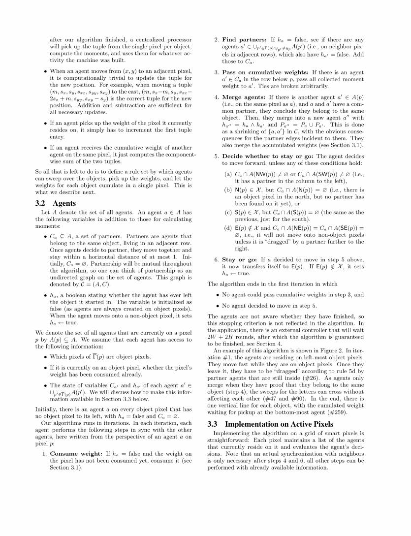
An example of this algorithm is shown in Figure 2. In iter-ation #1, the agents are residing on left-most object pixels.They move fast while they are on object pixels. Once theyleave it, they have to be “dragged” according to rule 5d bypartner agents that are still inside (#26). As agents onlymerge when they have proof that they belong to the sameobject (step 4), the sweeps for the letters can cross withoutaffecting each other (#47 and #90). In the end, there isone vertical line for each object, with the cumulated weightwaiting for pickup at the bottom-most agent (#259).
3.3 Implementation on Active PixelsImplementing the algorithm on a grid of smart pixels is
straightforward: Each pixel maintains a list of the agentsthat currently reside on it and evaluates the agent’s deci-sions. Note that an actual synchronization with neighborsis only necessary after steps 4 and 6, all other steps can beperformed with already available information.
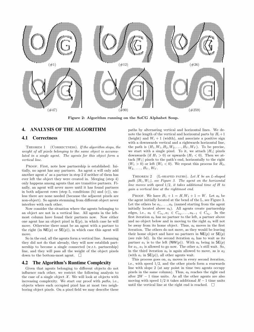
(#1) (#12) (#26)
(#47) (#90) (#259)
Figure 2: Algorithm running on the SoCG Alphabet Soup.
4. ANALYSIS OF THE ALGORITHM
4.1 Correctness
Theorem 1 (Correctness). If the algorithm stops, theweight of all pixels belonging to the same object is accumu-lated in a single agent. The agents for this object form avertical line.
Proof. First, note how partnership is established: Ini-tially, no agent has any partners. An agent a will only addanother agent a′ as a partner in step 2 if neither of them hasever left the object they were created in. Merging (step 4)only happens among agents that are transitive partners. Fi-nally, an agent will never move until it has found partnersin both adjacent rows (step 5, conditions (b) and (c)), un-less there are none needed (because the adjacent pixels arenon-object). So agents stemming from different object neverinterfere with each other.
Now consider the situation where the agents belonging toan object are not in a vertical line. All agents in the left-most column have found their partners now. Now eitherone agent has an object pixel in E(p), in which case he willmove. Otherwise there must be an agent with a partner tothe right (in NE(p) or SE(p)), in which case this agent willmove.
So in the end, all the agents form a vertical line. Assumingthey did not do that already, they will now establish part-nership to become a single connected (w.r.t. partnership)line, and they will pass all the weight of the object pixelsdown to the bottom-most agent.
4.2 The Algorithm’s Runtime ComplexityGiven that agents belonging to different objects do not
influence each other, we restrict the following analysis tothe case of a single object X . We will look at objects withincreasing complexity. We start our proof with paths, i.e.,objects where each occupied pixel has at most two neigh-boring object pixels. On a pixel field we may describe these
paths by alternating vertical and horizontal lines. We de-note the length of the vertical and horizontal parts by Hi +1(height) and Wi + 1 (width), and associate a positive signwith a downwards vertical and a rightwards horizontal line,the path is (H1,W1, H2,W2, . . . , HV ,WV ). To be precise,we start with a single pixel. To it, we attach |H1| pixelsdownwards (if H1 > 0) or upwards (H1 < 0). Then we at-tach |W1| pixels to the path’s end, horizontally to the right(W1 > 0) or left (W1 < 0). We repeat this process for H2,W2, . . . , HV , WV .
Theorem 2 (L-shaped paths). Let X be an L-shapedpath (H1,W1), see Figure 3. The agent on the horizontalline moves with speed 1/2, it takes additional time of H togain a vertical line at the rightmost end.
Proof. We have H1 + 1 = H,W1 + 1 = W . Let ab bethe agent initially located at the bend of the L, see Figure 3.Let the others be a1, . . . , ak (named starting from the agentinitially located above ab). All agents create partnershipedges, i.e., ab ∈ Ca1 , a1 ∈ Ca2 , . . . , ak−1 ∈ Cak . In thefirst iteration ab has no partner to the left, a partner aboveand no object below and in moving to the right ab will notbe away from its home object. Thus, ab moves in the firstiteration. The others do not move, as they would be leavingtheir home object and have no partners in NE(p) or SE(p)(see rule 5d). In the second iteration ab has to wait as itspartner a1 is to the left (NW(p)). With ab being in SE(p)for a1, a1 is allowed to go now. The other ai’s still wait. So,in the third iteration ab is again allowed to move, as is a2
(with a1 in SE(p)), all other agents wait.This process goes on, ab moves in every second iteration,
i.e., with speed 1/2, and the other pixels form a rearwardsline with slope 2 (at any point in time two agents occupypixels in the same column). Thus, ab reaches the right endafter 2W − 1 time units. As all the other agents are alsomoving with speed 1/2 it takes additional H − 1 time unitsuntil the vertical line at the right end is reached.
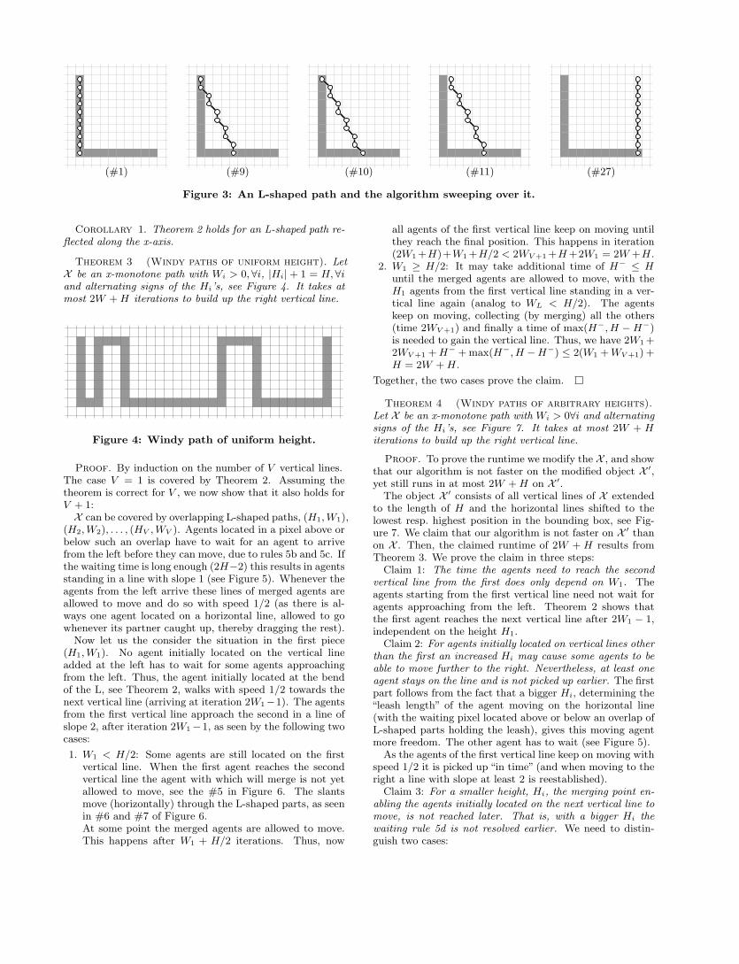
(#1) (#9) (#10) (#11) (#27)
Figure 3: An L-shaped path and the algorithm sweeping over it.
Corollary 1. Theorem 2 holds for an L-shaped path re-flected along the x-axis.
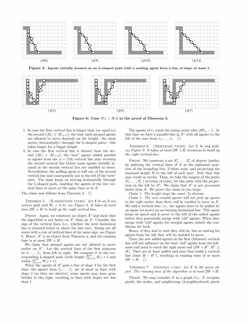
Theorem 3 (Windy paths of uniform height). LetX be an x-monotone path with Wi > 0, ∀i, |Hi|+ 1 = H, ∀iand alternating signs of the Hi’s, see Figure 4. It takes atmost 2W +H iterations to build up the right vertical line.
Figure 4: Windy path of uniform height.
Proof. By induction on the number of V vertical lines.The case V = 1 is covered by Theorem 2. Assuming thetheorem is correct for V , we now show that it also holds forV + 1:X can be covered by overlapping L-shaped paths, (H1,W1),
(H2,W2), . . . , (HV ,WV ). Agents located in a pixel above orbelow such an overlap have to wait for an agent to arrivefrom the left before they can move, due to rules 5b and 5c. Ifthe waiting time is long enough (2H−2) this results in agentsstanding in a line with slope 1 (see Figure 5). Whenever theagents from the left arrive these lines of merged agents areallowed to move and do so with speed 1/2 (as there is al-ways one agent located on a horizontal line, allowed to gowhenever its partner caught up, thereby dragging the rest).
Now let us the consider the situation in the first piece(H1,W1). No agent initially located on the vertical lineadded at the left has to wait for some agents approachingfrom the left. Thus, the agent initially located at the bendof the L, see Theorem 2, walks with speed 1/2 towards thenext vertical line (arriving at iteration 2W1−1). The agentsfrom the first vertical line approach the second in a line ofslope 2, after iteration 2W1−1, as seen by the following twocases:
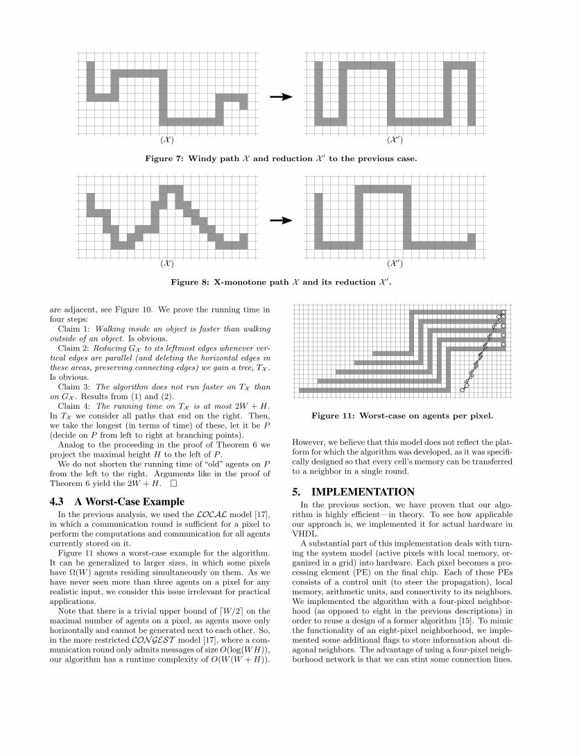
1. W1 < H/2: Some agents are still located on the firstvertical line. When the first agent reaches the secondvertical line the agent with which will merge is not yetallowed to move, see the #5 in Figure 6. The slantsmove (horizontally) through the L-shaped parts, as seenin #6 and #7 of Figure 6.At some point the merged agents are allowed to move.This happens after W1 + H/2 iterations. Thus, now
all agents of the first vertical line keep on moving untilthey reach the final position. This happens in iteration(2W1 +H)+W1 +H/2 < 2WV +1 +H+2W1 = 2W +H.
2. W1 ≥ H/2: It may take additional time of H− ≤ Huntil the merged agents are allowed to move, with theH1 agents from the first vertical line standing in a ver-tical line again (analog to WL < H/2). The agentskeep on moving, collecting (by merging) all the others(time 2WV +1) and finally a time of max(H−, H −H−)is needed to gain the vertical line. Thus, we have 2W1 +2WV +1 +H− + max(H−, H −H−) ≤ 2(W1 +WV +1) +H = 2W +H.
Together, the two cases prove the claim.
Theorem 4 (Windy paths of arbitrary heights).Let X be an x-monotone path with Wi > 0∀i and alternatingsigns of the Hi’s, see Figure 7. It takes at most 2W + Hiterations to build up the right vertical line.
Proof. To prove the runtime we modify the X , and showthat our algorithm is not faster on the modified object X ′,yet still runs in at most 2W +H on X ′.
The object X ′ consists of all vertical lines of X extendedto the length of H and the horizontal lines shifted to thelowest resp. highest position in the bounding box, see Fig-ure 7. We claim that our algorithm is not faster on X ′ thanon X . Then, the claimed runtime of 2W + H results fromTheorem 3. We prove the claim in three steps:
Claim 1: The time the agents need to reach the secondvertical line from the first does only depend on W1. Theagents starting from the first vertical line need not wait foragents approaching from the left. Theorem 2 shows thatthe first agent reaches the next vertical line after 2W1 − 1,independent on the height H1.
Claim 2: For agents initially located on vertical lines otherthan the first an increased Hi may cause some agents to beable to move further to the right. Nevertheless, at least oneagent stays on the line and is not picked up earlier. The firstpart follows from the fact that a bigger Hi, determining the“leash length” of the agent moving on the horizontal line(with the waiting pixel located above or below an overlap ofL-shaped parts holding the leash), gives this moving agentmore freedom. The other agent has to wait (see Figure 5).
As the agents of the first vertical line keep on moving withspeed 1/2 it is picked up “in time” (and when moving to theright a line with slope at least 2 is reestablished).
Claim 3: For a smaller height, Hi, the merging point en-abling the agents initially located on the next vertical line tomove, is not reached later. That is, with a bigger Hi thewaiting rule 5d is not resolved earlier. We need to distin-guish two cases:
(#6) (#8) (#10) (#12)
Figure 5: Agents initially located on an L-shaped path with a waiting agent form a line of slope at least 1.
(#5) (#6) (#7)
Figure 6: Case WL < H/2 in the proof of Theorem 3.
1. In case the first vertical line is longer than (or equal to)the second (|Hi| ≥ |Hi+1|), the time until merged agentsare allowed to move depends on the height: the slantmoves (horizontally) through the L-shaped parts—thistakes longer for a bigger height.
2. In case the first vertical line is shorter than the sec-ond (|Hi| < |Hi+1|), the “new” agents added parallelto agents from the (i + 1)th vertical line may overstepthe second vertical line before some agents initially lo-cated in the second vertical line are enabled to move.Nevertheless, the pulling agent is still one of the secondvertical line and consequently not to the left of the“new”ones. The slant keeps on moving horizontally throughthe L-shaped path, enabling the agents of the two ver-tical lines to move at the same time as in X .
The claim now follows from Theorem 3.
Theorem 5 (X-monotone paths). Let X be an X-mo-notone path with Wi > 0,∀i, see Figure 8. It takes at mosttime 2W +H to build up the right vertical line.
Proof. Again, we construct an object X ′ and show thatthe algorithm is not faster on X ′ than on X . Consider thesign of the vertical lines (i.e., whether the next horizontalline is situated below or above the last one). Swing out allstairs with a row of vertical lines of the same sign, see Figure8. Hence, X ′ is an object from Theorem 4, and the runningtime is at most 2W +H.
We claim that merged agents are not allowed to moveearlier on X ′. Let the vertical lines of the first staircasebe `1, . . . , `r, from left to right. We compare it to the cor-responding L-shaped path (with height (
Pri=1 Hi) + 1 and
width (Pr
i=1 Wi) + 1).When the agents of X ′ gain a line of slope 2 for the first
time, the agents from `1, . . . , `r are at most in lines withslope 2 (as they are shorter), some agents may have gonefurther to the right, resulting in lines with slopes not lessthan 1.
The agents of `1 reach the merge point after 2W`1 −1. Atthis time we have a parallel line in X ′ with all agents to theleft of the ones from `1, . . . , `r.
Theorem 6 (Arbitrary paths). Let X be any path,see Figure 9. It takes at most 2W +H iterations to build upthe right vertical line.
Proof. We construct a set X ′1, . . . ,X ′z of objects (paths)by splitting the vertical lines of X at the rightmost posi-tion of the bounding box, if these exist, and projecting themaximal height H to the left of each part. Note that thismay result in circles. Then, we take the longest of the pathsX ′1, . . . ,X ′z ( in terms of time), let this path with the projec-tion on the left be X ′. We claim that X ′ is not processedfaster than X . We prove the claim in two steps:
Claim 1: The height stays the same. Is obvious.Claim 1: The new created agents will not pick up agents
to the right earlier than these will be enabled to move in X .We add a vertical line, i.e., the agents have to be pulled byan agent (or more) on an existing horizontal line. This agentkeeps its speed and is never to the left of the added agentsbefore they potentially merge with “old” agents: When theymerge with “old” agents the merged agents inherit the con-ditions for both.
Hence, if they had to wait they still do, but as waiting foragents from the left they will be enabled to move.
Thus, the new added agents on the first (leftmost) verticalline will not influence on the time “old” agents from the left-most end need to reach the right most end (2W +H∗, H∗ ≤H). They are at least pulled and may then build a verticalline (time H − H∗), resulting in running time of at most2W +H.
Theorem 7 (General case). Let X be the given ob-ject. The running time of the algorithm is at most 2W +H.
Proof. We may consider X as a graph GX : X occupiespixels, the nodes, and neighboring (4-neighborhood) pixels
(X ) (X ′)
Figure 7: Windy path X and reduction X ′ to the previous case.
(X ) (X ′)
Figure 8: X-monotone path X and its reduction X ′.
are adjacent, see Figure 10. We prove the running time infour steps:
Claim 1: Walking inside an object is faster than walkingoutside of an object. Is obvious.
Claim 2: Reducing GX to its leftmost edges whenever ver-tical edges are parallel (and deleting the horizontal edges inthese areas, preserving connecting edges) we gain a tree, TX .Is obvious.
Claim 3: The algorithm does not run faster on TX thanon GX . Results from (1) and (2).
Claim 4: The running time on TX is at most 2W + H.In TX we consider all paths that end on the right. Then,we take the longest (in terms of time) of these, let it be P(decide on P from left to right at branching points).
Analog to the proceeding in the proof of Theorem 6 weproject the maximal height H to the left of P .
We do not shorten the running time of “old” agents on Pfrom the left to the right. Arguments like in the proof ofTheorem 6 yield the 2W +H.
4.3 A Worst-Case ExampleIn the previous analysis, we used the LOCAL model [17],
in which a communication round is sufficient for a pixel toperform the computations and communication for all agentscurrently stored on it.
Figure 11 shows a worst-case example for the algorithm.It can be generalized to larger sizes, in which some pixelshave Ω(W ) agents residing simultaneously on them. As wehave never seen more than three agents on a pixel for anyrealistic input, we consider this issue irrelevant for practicalapplications.
Note that there is a trivial upper bound of dW/2e on themaximal number of agents on a pixel, as agents move onlyhorizontally and cannot be generated next to each other. So,in the more restricted CONGEST model [17], where a com-munication round only admits messages of sizeO(log(WH)),our algorithm has a runtime complexity of O(W (W +H)).
Figure 11: Worst-case on agents per pixel.
However, we believe that this model does not reflect the plat-form for which the algorithm was developed, as it was specifi-cally designed so that every cell’s memory can be transferredto a neighbor in a single round.
5. IMPLEMENTATIONIn the previous section, we have proven that our algo-
rithm is highly efficient—in theory. To see how applicableour approach is, we implemented it for actual hardware inVHDL.
A substantial part of this implementation deals with turn-ing the system model (active pixels with local memory, or-ganized in a grid) into hardware. Each pixel becomes a pro-cessing element (PE) on the final chip. Each of these PEsconsists of a control unit (to steer the propagation), localmemory, arithmetic units, and connectivity to its neighbors.We implemented the algorithm with a four-pixel neighbor-hood (as opposed to eight in the previous descriptions) inorder to reuse a design of a former algorithm [15]. To mimicthe functionality of an eight-pixel neighborhood, we imple-mented some additional flags to store information about di-agonal neighbors. The advantage of using a four-pixel neigh-borhood network is that we can stint some connection lines.
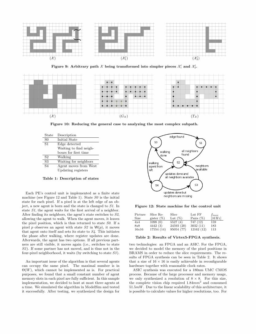
(X ) (X ′1) (X ′2)
Figure 9: Arbitrary path X being transformed into simpler pieces X ′1 and X ′2.
(X ) (GX ) (TX )
Figure 10: Reducing the general case to analyzing the most complex subpath.
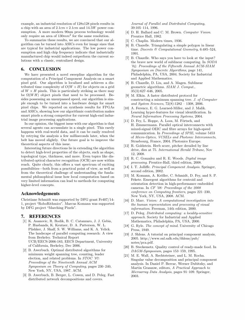
State DescriptionS0 Initial StateS1 Edge detected
Waiting to find neigh-bours for first time
S2 WalkingS3 Waiting for neighborsS4 Agent moves from West
Updating registers
Table 1: Description of states
Each PE’s control unit is implemented as a finite statemachine (see Figure 12 and Table 1). State S0 is the initialstate for each pixel. If a pixel is at the left edge of an ob-ject, a new agent is born and the state is changed to S1. Instate S1, the agent waits for the first arrival of a neighbor.After finding its neighbors, the agent’s state switches to S2,allowing the agent to walk. When the agent moves, it leavesthe pixel position, which is thus returned to state S0. If apixel p observes an agent with state S2 in W(p), it movesthat agent onto itself and sets its state to S4. This initiatesthe phase after walking, where register updates are done.Afterwards, the agent has two options. If all previous part-ners are still visible, it moves again (i.e., switches to stateS2 ). If some partner has not moved, and is thus not in thefour-pixel neighborhood, it waits (by switching to state S3 ).
An important issue of the algorithm is that several agentscan occupy the same pixel. The maximal number is inΘ(W ), which cannot be implemented as is. For practicalpurposes, we found that a small constant number of agentmemory slots in each pixel are fully sufficient. In this sampleimplementation, we decided to host at most three agents ata time. We simulated the algorithm in ModelSim and testedit successfully. After testing, we synthesized the design for
Figure 12: State machine for the control unit
Picture Slice Re- Slice Lut FF fmax
Size gister (%) Lut (%) Pairs (%) [MHz]4x4 1098 (0) 5527 (4) 747 (12) 1598x8 4442 (3) 24593 (20) 3032 (11) 18316x16 17554 (14) 95054 (77) 12162 (12) 113
Table 2: Results of Virtex5-FPGA synthesis.
two technologies: an FPGA and an ASIC. For the FPGA,we decided to model the memory of the pixel positions inBRAMS in order to reduce the slice requirements. The re-sults of FPGA synthesis can be seen in Table 2. It showsthat a size of 16 × 16 is easily achievable in reconfigurablehardware together with reasonable clock rates.
ASIC synthesis was executed for a 180nm UMC CMOSprocess. Because of the large processor and memory usage,we only synthesized a resolution of 8 × 8. For this size,the complete vision chip required 1.84mm2 and consumed51.5mW . Due to the linear scalability of this architecture, itis possible to calculate values for higher resolutions, too. For
example, an industrial resolution of 128x128 pixels results ina chip with an area of 2.1cm×2.1cm and 14.5W power con-sumption. A more modern 90nm process technology wouldonly require an area of 130mm2 for the same resolution.
To summarize these results, we are convinced that our al-gorithm can be turned into ASICs even for image sizes thatare typical for industrial applications. The low power con-sumption and high chip frequency indicate that industriallymanufactured chip would indeed outperform the current so-lutions with a classic, centralized design.
6. CONCLUSIONWe have presented a novel sweepline algorithm for the
computation of a Principal Component Analysis on a smartpixel grid. Our algorithm is localized and achieves a dis-tributed time complexity of O(W +H) for objects on a gridof W ×H pixels. This is particularly striking as there maybe Ω(WH) object pixels that need to be processed. Be-sides possessing an unsurpassed speed, our algorithm is sim-ple enough to be turned into a hardware design for smartpixel chips. We reported on synthesis results for FPGAsand ASICs, showing how our algorithmic contribution makessmart pixels a strong competitor for current high-end indus-trial image processing applications.
In our opinion, the biggest issue with our algorithm is thatseveral agents can accumulate in a single pixel. This rarelyhappens with real-world data, and it can be easily resolvedby retrying the analysis a few milliseconds later, when thebelt has moved slightly. Our future goal is to improve thetheoretical aspects of this issue.
Interesting future directions lie in extending the algorithmto detect high-level properties of the objects, such as shape,topological type, thickness, and more. Even topics like dis-tributed optical character recognition (OCR) are now withinreach. Quite clearly, this offers a vast spectrum of excitingpossibilities—both from a practical point of view, as well asfrom the theoretical challenge of understanding the funda-mental philosophical issue how local computation based onvery limited information can lead to methods for computinghigher-level concepts.
AcknowledgementsChristiane Schmidt was supported by DFG grant Fe407/14-1, project “RoboRithmics”. Marcus Komann was supportedby DFG project “Marching Pixels”.
7. REFERENCES[1] K. Asanovic, R. Bodik, B. C. Catanzaro, J. J. Gebis,
P. Husbands, K. Keutzer, D. A. Patterson, W. L.Plishker, J. Shalf, S. W. Williams, and K. A. Yelick.The landscape of parallel computing research: A viewfrom Berkeley. Technical ReportUCB/EECS-2006-183, EECS Department, Universityof California, Berkeley, Dec 2006.
[2] B. Awerbuch. Optimal distributed algorithms forminimum weight spanning tree, counting, leaderelection, and related problems. In STOC ’87:Proceedings of the Nineteenth Annual ACMSymposium on Theory of Computing, pages 230–240,New York, NY, USA, 1987. ACM.
[3] B. Awerbuch, B. Berger, L. Cowen, and D. Peleg. Fastdistributed network decompositions and covers.
Journal of Parallel and Distributed Computing,39:105–114, 1996.
[4] D. H. Ballard and C. M. Brown. Computer Vision.Prentice Hall, 1982.
[5] C. Chaplin. Modern times, 1936.
[6] B. Chazelle. Triangulating a simple polygon in lineartime. Discrete & Computational Geometry, 6:485–524,1991.
[7] B. Chazelle. Who says you have to look at the input?the brave new world of sublinear computing. In SODA’04: Proceedings of the Fifteenth Annual ACM-SIAMSymposium on Discrete Algorithms, page 141,Philadelphia, PA, USA, 2004. Society for Industrialand Applied Mathematics.
[8] B. Chazelle, D. Liu, and A. Magen. Sublineargeometric algorithms. SIAM J. Comput.,35(3):627–646, 2005.
[9] M. Elkin. A faster distributed protocol forconstructing a minimum spanning tree. J. of Computerand System Sciences, 72(8):1282 – 1308, 2006.
[10] A. Ferencz, E. G. Learned-Miller, and J. Malik.Learning hyper-features for visual identification. InNeural Information Processing Systems, 2004.
[11] D. Fey, L. Hoppe, A. Loos, M. Fortsch, andH. Zimmermann. Parallel optical interconnects withmixed-signal OEIC and fibre arrays for high-speedcommunication. In Proceedings of SPIE, volume 5453of Micro-Optics, VCSELs and Photonic Interconnects,Strasbourg, France, 2004. Photonics Europe.
[12] R. Goldstein. Herb score, pitcher derailed by linedrive, dies at 75. International Herald Tribune, Nov12, 2008.
[13] R. C. Gonzalez and R. E. Woods. Digital imageprocessing. Prentice-Hall, third edition, 2008.
[14] I. T. Jolliffe. Principal Component Analysis. Springer,second edition, 2002.
[15] M. Komann, A. Kroller, C. Schmidt, D. Fey, and S. P.Fekete. Emergent algorithms for centroid andorientation detection in high-performance embeddedcameras. In CF ’08: Proceedings of the 2008conference on Computing frontiers, pages 221–230,New York, NY, USA, 2008. ACM.
[16] D. Marr. Vision: A computational investigation intothe human representation and processing of visualinformation. Freeman, 14th edition, 2000.
[17] D. Peleg. Distributed computing: a locality-sensitiveapproach. Society for Industrial and AppliedMathematics, Philadelphia, PA, USA, 2000.
[18] G. Ryle. The concept of mind. University of ChicagoPress, 1949.
[19] J. Shlens. A tutorial on principal component analysis,2005. http://www.snl.salk.edu/shlens/pub/notes/pca.pdf.
[20] B. Steckemetz. Quality control of ready-made food. InDAGM-Symposium, pages 153–159, 1995.
[21] M. E. Wall, A. Rechtsteiner, and L. M. Rocha.Singular value decomposition and principal componentanalysis. In Daniel P. Berrar, Werner Dubitzky, andMartin Granzow, editors, A Practical Approach toMicroarray Data Analysis, pages 91–109. Springer,2003.