�����������������

Citation: Kashani, M.; Hashemi, S.M.

Dynamic Finite Element Modelling

and Vibration Analysis of Prestressed

Layered Bending–Torsion Coupled

Beams. Appl. Mech. 2022, 3, 103–120.

https://doi.org/10.3390/

applmech3010007

Received: 28 July 2021

Accepted: 12 January 2022

Published: 16 January 2022

Publisher’s Note: MDPI stays neutral

with regard to jurisdictional claims in

published maps and institutional affil-

iations.

Copyright: © 2022 by the authors.

Licensee MDPI, Basel, Switzerland.

This article is an open access article

distributed under the terms and

conditions of the Creative Commons

Attribution (CC BY) license (https://

creativecommons.org/licenses/by/

4.0/).

Article

Dynamic Finite Element Modelling and Vibration Analysis ofPrestressed Layered Bending–Torsion Coupled BeamsMirTahmaseb Kashani and Seyed M. Hashemi *

Department of Aerospace Engineering, Ryerson University, Toronto, ON M5B 2K3, Canada; tahmaseb@ryerson.ca* Correspondence: smhashem@ryerson.ca; Tel.: +1-416-979-5000 (ext. 556421)

Abstract: Free vibration analysis of prestressed, homogenous, Fiber-Metal Laminated (FML) andcomposite beams subjected to axial force and end moment is revisited. Finite Element Method (FEM)and frequency-dependent Dynamic Finite Element (DFE) models are developed and presented. Thefrequency results are compared with those obtained from the conventional FEM (ANSYS, Canons-burg, PA, USA) as well as the Homogenization Method (HM). Unlike the FEM, the application of theDFE formulation leads to a nonlinear eigenvalue problem, which is solved to determine the system’snatural frequencies and modes. The governing differential equations of coupled flexural–torsional vi-brations, resulting from the end moment, are developed using Euler–Bernoulli bending and St. Venanttorsion beam theories and assuming linear harmonic motion and linearly elastic materials. Illustrativeexamples of prestressed layered, FML, and unidirectional composite beam configurations, exhibitinggeometric bending-torsion coupling, are studied. The presented DFE and FEM results show excellentagreement with the homogenization method and ANSYS modeling results, with the DFE’s rates ofconvergence surpassing all. An investigation is also carried out to examine the effects of variouscombined axial loads and end moments on the stiffness and fundamental frequencies of the structure.An illustrative example, demonstrating the application of the presented methods to the bucklinganalysis of layered beams is also presented.

Keywords: coupled vibration; layered beam; prestress; dynamic finite element; FEM

1. Introduction

Vibration is one of the main causes of structural failure, which makes it one of the mostimportant and ongoing research fields in structural modelling and analysis. Multilayeredstructures, with their increasing applications in aerospace, mechanical and civil engineering,are subjected to different types of preloads based on their application. One of these prestressconditions is combined axial force and end moment which, for instance, happens wherestructural members are interconnected through an imperfect joint. Layered and laminatedcomposite materials, e.g., Fiber-Metal Laminates (FMLs), are more prone to failure underthese conditions due to their manufacturing nature. FML materials consist of layers of metalsheet and unidirectional fiber layers embedded in an adhesive system. Glare, an optimizedFML with increasing applications in aircraft manufacturing, consists of alternating layersof aluminum and glass fiber prepreg layers.

The governing differential equations describing the motion for many beam configura-tions have been already developed and reported in the literatures. Neogy and Murthy [1]carried out one of the earliest studies around prestressed beams and found the fundamentalfrequency of an axially loaded column for two different boundary conditions of pinned-pinned and clamped-clamped. Prasad et al. [2] introduced a solution using Rayleigh-Ritzprinciples in an iterative form, and in comparison, with other approximate methods.

The bending-torsion coupled vibration of beams caused by cross-sectional geometrywas first addressed by Timoshenko [3] and has been further studied by, among many

Appl. Mech. 2022, 3, 103–120. https://doi.org/10.3390/applmech3010007 https://www.mdpi.com/journal/applmech

Appl. Mech. 2022, 3 104

other researchers, the second author (and his co-workers) to develop new solution meth-ods, or to include diverse effects such as axial load (see, for example, [4,5]). Materiallycoupled vibrations of beams caused by different material couplings [6,7] have also beenaddressed and the governing differential equations describing the motion of various beamconfigurations have been developed [8,9]. Stability and vibrational analyses of beamssubjected to axial preload and its effects on the beam stiffness and elasticity have also beenconducted [10,11]. However, the vibration analysis of beams subjected to combined axialforce and end moment is scarce [12–14].

Many analytical, semi-analytical and numerical methods have been developed to findsolutions to the governing differential equations of motion. The Finite Element Method(FEM), as the most popular computational method in structural mechanics, has beenextensively implemented by researchers (see, for example, [15–17]). Analytical solutionshave also been formulated for the vibration analysis of various beam configurations [11,15]and Banerjee et al. [18] presented a Dynamic Stiffness Matrix (DSM) for coupled bending–torsion beam elements. Hashemi [19] introduced the frequency-dependent Dynamic FiniteElement (DFE) method, a hybrid method bridging the gap between the conventionalFEM and DSM methods. The DFE combines the accuracy of analytical methods with theversatility of numerical methods to conduct a vibration analysis of structural elementsexhibiting coupled behaviours. The DFE formulation has since been further extended tovibration analysis of more complex beam configurations (see, for example [4–7]).

More recently, Ahmet Hasim [20] presented an isogeometric refined zigzag finiteelement (IGRZF) model that gives the opportunity to obtain the exact beam geometriesdirectly from a computer aided design (CAD) software, Rhinoceros. The employed kine-matics is based on the refined zigzag theory that makes the finite element independentfrom the number of layers considered. In this method, not only the element does not sufferfrom shear locking and geometric error, but it also does not need shear correction factors.The presented IGRZF approach is then used to analyze various sandwich beams. Later,Kefal et al. [21] extended this method to perform quasi-static structural analysis of sandwichand laminated composite beams with embedded delamination. An incomplete interac-tion, leading to interlayer slip, has also been considered and modeled. Foraboschi [22]introduced a 2D mathematical model for a two-layer beam, considering interlayer slip.Cas et al. [23] presented a derivation of a new mathematical model and its analytical solu-tion for the analysis of geometrically and materially linear, 3D, two-layer, composite beams,with interlayer slips between the layers for the first time. In this study, it is assumed thatthere is no incomplete interaction between the layers.

Cortés and Sarría [24] presented a dynamic analysis of 3-Layer sandwich beams withthick viscoelastic damping core for FEM applications. They introduced a modified RKUmodel [25]. RKU model, originally proposed by Ross, Kerwin and Ungar [25] for thevibration modeling of viscoelastic laminate, is one of the first methods developed to findthe flexural stiffness of sandwich beams and it is still commonly used in engineeringapplications because of its ease of computational implementation. Although RKU appliesto simply supported beams it has been used for other types of boundary conditions aswell. Besides other boundary conditions, Cortés and Sarría [24] used RKU for the dynamicanalysis of cantilevered sandwich beams.

There are many studies on other aspects of the beam’s dynamics and stability.Mohri et al. [26] studied the vibration of buckled thin-walled beams with open sections.They dealt with small, superimposed vibrations of thin-walled elements with variousopen sections such as bisymmetric sections. They investigated vibration under two typesof static pre-loadings: pure compression and lateral bending forces. A nonlinear modelwhich accounts for nonlinear warping, bending-bending and torsion-bending couplingswas used for the analysis. Franzoni et al. [27] proposed a numerical approach, based on anonlinear finite element model and an experimental modal analysis procedure, to estimatethe dynamic behavior of a typical aeronautical aluminum box-beam structure liable tobuckling. Augello et al. [28] proposed an efficient Carrera Unified Formulation (CUF)-

Appl. Mech. 2022, 3 105

based method for the vibrations and buckling of thin-walled open cross-section beams,with complex geometries, under progressive compressive loads. A comprehensive studywas also conducted in order to investigate the effects of compressive loads on the naturalfrequencies of the thin-walled beams. Namely, a numerical simulation of the VibrationCorrelation Technique was provided. Finite Elements were built in the framework of theCUF, and the displacements of complex geometric shapes of the thin-walled beams wereevaluated using low- to higher-order Taylor and Lagrange polynomials.

As mentioned earlier, the coupled free vibration analysis of homogeneous beamssubjected to combined axial force and end moment has only been investigated in a fewsemi-analytical studies [12–14]. The geometrically coupled flexural–torsional vibration ofhomogeneous beams caused by combined prestress was recently revisited by the authors,using both FEM and DFE methods [29–31]. To the authors’ best knowledge, the geometri-cally coupled flexural–torsional vibration of layered beams, in the presence of combinedaxial load and end moment has not been reported in the open literature. In what follows,the coupled flexural–torsional vibration of axially-loaded layered beams, caused by theend moment is investigated and two formulations are presented.

The presented mathematical model is based on some simplifying assumptions, whichlead to computational benefits for the presented methods. An equivalent single-layerformulation, similar to that presented in the RKU model and used by Cortés and Sarría [24],is exploited. The equivalent single-layer model is then discretized (along the beam length)using FEM [29,31] and DFE [30]. The application of the presented theory is demonstratedthrough the vibration analysis of illustrative prestressed layered beams. The presentedlayered FEM and DFE results show excellent agreement with homogenization methodand ANSYS modeling results, with the DFE’s rates of convergence surpassing all. Aninvestigation is also carried out to examine the effects of various combined axial loads andend moments on the stiffness and fundamental frequencies of the structure. An illustrativeexample, demonstrating the application of the presented methods to the buckling analysisof layered beams is also presented.

The structure of the paper is as follows: In Section 2, the concept of coupled, linear,undamped, free vibration of prestressed multi-layer beam, is presented followed by theexpressions for the Galerkin-type integral form of the governing differential equations.Next, two layered beam conventional FEM (LBFEM) and Dynamic, frequency dependent(LBDFE) formulations are presented. In Section 3, the application of presented formulationsto four cases of Steel-rubber-steel layered beam (Section 3.1), Cantilever Three-layeredFiber-Metal Laminated (FML) Beam (Section 3.2), and Cantilever Three-layered LaminatedComposite Beam (Section 3.3), are presented. In Section 4, a discussion of the resultsobtained is provided followed by final conclusions that summarize the most importantachievements of the article.

2. Materials and Methods

Consider a (three-)layered beam subjected to two equal and opposite end moments,Mzz, about z-axis and an axial load, P, loaded in the plane of greater bending rigidity,undergoing linear coupled torsion and lateral vibrations along the z-axis. Figure 1 depictsthe schematic of the problem, where L, h and t stand for the beam’s length, width andheight, respectively. As mentioned earlier, the presented mathematical model is basedon an equivalent single-layer formulation, similar to that presented in the RKU modeland used in [24]. The equivalent single-layer model is discretized (along the beam length)using FEM [29,31] and DFE [30]. The flexural and torsional rigidities of the equivalentsingle-layer beam are obtained by the addition of the individual contribution of each layer(calculated with respect to the beam neutral axis) [24,28]. It is assumed that the equivalentsingle-layer beam undergoes bending and torsional displacements and vibrates in a waylike the original layered configuration, i.e., dynamically equivalent. One might put thisin an overly simplistic way by saying all layers exhibit the same transverse displacement,slope, and torsional rotation. However, in reality this would violate interlayer lateral and

Appl. Mech. 2022, 3 106

axial displacements’ continuity and the use of a beam model accounting for 3D motion ispreferable. Even so, the equivalent single-layer model in the vibration analysis of layeredbeams is commonly used [24,25].

Appl. Mech. 2022, 3 106

like the original layered configuration, i.e., dynamically equivalent. One might put this in an overly simplistic way by saying all layers exhibit the same transverse displacement, slope, and torsional rotation. However, in reality this would violate interlayer lateral and axial displacements’ continuity and the use of a beam model accounting for 3D motion is preferable. Even so, the equivalent single-layer model in the vibration analysis of layered beams is commonly used [24,25].

For composite layers, the lamina theory and the method of homogenization are first used to find the equivalent physical properties of each layer, which are then used to obtain the equivalent single-layer beam model. Exploiting the classical lamination theory, a ho-mogenized beam model is also developed and is used for the validation purposes. In this case, the apparent material properties (equivalent ρ, E, G, …) are used to treat the original layered beam as a simple beam. Consequently, only one set of (two coupled) equations of motion, with the homogenized parameters are solved. In contrast, the equivalent single-layer model uses equivalent flexural and torsional rigidities obtained and three sets of equations (six equations in total), combined as two, are solved.

Governing differential equations of motion is developed by defining an infinitesimal element using the following assumptions: 1. The displacements are small. 2. The stresses induced are within the limit of proportionality. 3. The cross–section of the beam has two axes of symmetry. 4. The cross–sectional dimensions of the beam are small compared to the span. 5. The transverse cross–sections of the beam remain plane and normal to the neutral

axis during bending, and 6. The beam’s torsional rigidity (GJ) is assumed to be very large compared with its

warping rigidity (EΓ), and ends are free to warp, i.e., state of uniform torsion. 7. Damping is neglected.

(a) (b)

Figure 1. 3-Layered Beam, with axial load and end-moment applied at x = 0 and x = L; Sf represents transverse shearing force. (a) The loads on an element of beam of length δx, and (b) The coordinate system and loadings.

Using the above-mentioned assumptions, it can be shown [12,26] that the governing differential equations for a prismatic, Euler–Bernoulli beam (EI = constant) subjected to constant axial force (P) and end moment (Mzz), and undergoing coupled flexural-torsional vibrations (caused by end moment), are as follows: 𝐸𝐼𝑤′′′′ + 𝑃𝑤′′ + 𝑀 𝜃′′ − 𝜌𝐴𝑤 = 0 (1) 𝐺𝐽𝜃′′ + 𝑃𝐼𝐴 𝜃′′ + 𝑀 𝑤” − 𝜌𝐼 𝜃 = 0 (2)

where ()′, stands for derivative with respect to x and (•) denotes derivative with respect to t (time). As can be observed from Equations (1) and (2), the system is coupled by the end-moments, Mzz. The pre-stress effects of axial load and end moment are represented by the second and third terms in Equations (1) and (2). These coupling rigidities will result in a (coupling) stiffness matrix which represents the pre-stress effects on the beam’s rigidity.

Exploiting the simple harmonic motion assumption, displacements, w and θ, are written as:

Figure 1. 3-Layered Beam, with axial load and end-moment applied at x = 0 and x = L; Sf representstransverse shearing force. (a) The loads on an element of beam of length δx, and (b) The coordinatesystem and loadings.

For composite layers, the lamina theory and the method of homogenization are firstused to find the equivalent physical properties of each layer, which are then used to obtainthe equivalent single-layer beam model. Exploiting the classical lamination theory, ahomogenized beam model is also developed and is used for the validation purposes. In thiscase, the apparent material properties (equivalent ρ, E, G, . . . ) are used to treat the originallayered beam as a simple beam. Consequently, only one set of (two coupled) equations ofmotion, with the homogenized parameters are solved. In contrast, the equivalent single-layer model uses equivalent flexural and torsional rigidities obtained and three sets ofequations (six equations in total), combined as two, are solved.

Governing differential equations of motion is developed by defining an infinitesimalelement using the following assumptions:

1. The displacements are small.2. The stresses induced are within the limit of proportionality.3. The cross–section of the beam has two axes of symmetry.4. The cross–sectional dimensions of the beam are small compared to the span.5. The transverse cross–sections of the beam remain plane and normal to the neutral

axis during bending, and6. The beam’s torsional rigidity (GJ) is assumed to be very large compared with its

warping rigidity (EΓ), and ends are free to warp, i.e., state of uniform torsion.7. Damping is neglected.

Using the above-mentioned assumptions, it can be shown [12,26] that the governingdifferential equations for a prismatic, Euler–Bernoulli beam (EI = constant) subjected toconstant axial force (P) and end moment (Mzz), and undergoing coupled flexural-torsionalvibrations (caused by end moment), are as follows:

EIw′′′′ + Pw′′ + Mzzθ′′ − ρA..w = 0 (1)

GJθ′′ +PIPA

θ′′ + Mzzw′′ − ρIP..θ = 0 (2)

where ()′, stands for derivative with respect to x and (•) denotes derivative with respectto t (time). As can be observed from Equations (1) and (2), the system is coupled by theend-moments, Mzz. The pre-stress effects of axial load and end moment are represented bythe second and third terms in Equations (1) and (2). These coupling rigidities will result ina (coupling) stiffness matrix which represents the pre-stress effects on the beam’s rigidity.

Appl. Mech. 2022, 3 107

Exploiting the simple harmonic motion assumption, displacements, w and θ, arewritten as:

w(x, t) = Wsin(ωt), (3)

θ(x, t) = θsin(ωt), (4)

where ω denotes the frequency, W and θ are the amplitudes of flexural and torsionaldisplacements, respectively. Substituting Equations (3) and (4) into Equations (1) and (2)leads to:

EIW ′′′′ + PW ′′ + Mzz θ′′ − ρAω2W = 0 (5)

GJθ′′ + PIP θ′′ + MzzW ′′ − ρIP Aω2θ = 0 (6)

As, in this case, there are three layers with different materials, one will have three setsof equations, i.e., two for each layer and six equations in total, written as (I = 1, 2, 3):

EIW ′′′′ + PW ′′ + Mzz θ′′ − ρAω2W = 0 (7)

Gi Ji θ′′i + Pi IP,i θ

′′i + Mzz,iW

′′i − ρi IP,i Aiω

2θi = 0 (8)

where indices 1, 2 and 3 represent the properties of layer 1, layer 2 and layer 3, respectively.The second moment of inertia and polar moment of inertia for each layer is calculated aboutthe neutral axis of the whole (beam) cross–section, and axial force and moment equilibriumequations are written as:

P = P1 + P2 + P3, and Mzz = Mzz,1 + Mzz,2 + Mzz,3 (9)

It is worth noting that Equations (7) and (8) can be readily extended to n-layer beamconfigurations (i.e., I = 1, 2, . . . , n). Assuming linearly elastic materials, an equivalentsingle-layer beam model [24,28] is developed, which vibrates in a similar way as the originallayered configuration. The equivalent single-layer beam, governed by the pair of coupledEquations (7) and (8), undergoes bending displacement, W, and torsional displacement, θ.Simply put, the lateral and torsional displacements and slope of all layers are set equal (likeANSYS ‘constraint rigid link’ element [32]); i.e., W1 = W2 = W3 = W and θ1 = θ2 = θ3 = θ.In other words, the summation of three bending equations describes the bending equationof the whole beam and the summation of three torsion equations describes the torsionequation of the equivalent single-layer beam, resulting in the following two through-the-thickness equations:

(E1 I1 + E2 I2 + E3 I3)W ′′′′ + (P1 + P2 + P3)W ′′ + (Mzz,1 + Mzz,2 + Mzz,3)θ′′

−(ρ1 A1 + ρ2 A2 + ρ3 A3)ω2W = 0,

(10)

(G1 J1 + G2 J2 + G3 J3)θ′′ + (P1 IP,1 + P2 IP,2 + P3 IP,3)θ′′ + (Mzz,1 + Mzz,2 + Mzz,3)W ′′

−(ρ1 IP,1 A1 + ρ2 IP,2 A2 + ρ3 IP,3 A3)ω2θ = 0,

(11)

where the bending and torsional rigidities of all layers (EiIi, and GiJi, i = 1, 2, 3, in this case.)are calculated with respect to the neutral axis of the overall cross–sectional area. In otherwords, as previously mentioned, the addition terms of flexural and torsional rigidities,(E1I1 + E2I2 + E3I3) and (G1J1 + G2J2 + G3J3), respectively, represent the correspondingrigidities for the equivalent single-layer beam model [24,28].

The Galerkin method of weighted residuals is employed to develop the integral formof the above equations, written as (note: from this point on, the hat sign has been omittedfor simplicity):

Appl. Mech. 2022, 3 108

W f =∫ L

0δW((E1 I1 + E2 I2 + E3 I3)W ′′′′ + (P1 + P2 + P3)W ′′ + (Mzz,1 + Mzz,2 + Mzz,3)θ′′−

(ρ1 A1 + ρ2 A2 + ρ3 A3)ω2W)

dx = 0(12)

Wt =∫ L

0δθ((G1 J1 + G2 J2 + G3 J3)θ′′ + (P1 IP,1 + P2 IP,2 + P3 IP,3)θ′′ + (Mzz,1 + Mzz,2 + Mzz,3)W ′′−

(ρ1 IP,1 A1 + ρ2 IP,2 A2 + ρ3 IP,3 A3)ω2θ)

dx = 0(13)

where δW and δθ (i.e., weighting functions) represent the transverse and torsional virtualdisplacements, respectively. Performing integration by parts on Equations (12) and (13)leads to the weak integral form of the governing equations, where the resulting boundaryterms vanish irrespective of boundary conditions [33]. The beam is then discretized alongits length (see Figure 2), leading to the following element integral equations:

Wkf =

∫ l

0

((E1 I1 + E2 I2 + E3 I3)W ′′ δW ′′ + (P1 + P2 + P3)W ′δW ′+

(Mzz,1 + Mzz,2 + Mzz,3)θ′δW ′ − (ρ1 A1 + ρ2 A2 + ρ3 A3)ω

2WδW)

dx(14)

Wkt =

∫ l

0

((G1 J1 + G2 J2 + G3 J3)θ

′δθ′ + (P1 IP,1 + P2 IP,2 + P3 IP,3)θ′δθ′+

(Mzz,1 + Mzz,2 + Mzz,3)W ′δθ′ − (ρ1 IP,1 A1 + ρ2 IP,2 A2 + ρ3 IP,3 A3)ω2θδθ

)dx

(15)

Appl. Mech. 2022, 3 108

where δW and δθ (i.e., weighting functions) represent the transverse and torsional virtual displacements, respectively. Performing integration by parts on Equations (12) and (13) leads to the weak integral form of the governing equations, where the resulting boundary terms vanish irrespective of boundary conditions [33]. The beam is then discretized along its length (see Figure 2), leading to the following element integral equations: 𝑊 = (𝐸 𝐼 + 𝐸 𝐼 + 𝐸 𝐼 )𝑊 𝛿𝑊′′ + (𝑃 + 𝑃 + 𝑃 )𝑊 𝛿𝑊′ +𝑀 , + 𝑀 , + 𝑀 , 𝜃 𝛿𝑊′ − (𝜌 𝐴 + 𝜌 𝐴 + 𝜌 𝐴 )𝜔 𝑊𝛿𝑊 𝑑𝑥

(14)

𝑊 = (𝐺 𝐽 + 𝐺 𝐽 + 𝐺 𝐽 )𝜃 𝛿𝜃′ + (𝑃 𝐼 , + 𝑃 𝐼 , + 𝑃 𝐼 , )𝜃 𝛿𝜃′ +𝑀 , + 𝑀 , + 𝑀 , 𝑊 𝛿𝜃′ − 𝜌 𝐼 , 𝐴 + 𝜌 𝐼 , 𝐴 + 𝜌 𝐼 , 𝐴 𝜔 𝜃𝛿𝜃 𝑑𝑥 (15)

The above expressions (14) and (15), also satisfies the principle of virtual work (𝑊 = 𝑊 + 𝑊 = 0, with 𝑊 = 0, for free vibrations), where: 𝑊 = 𝑊 = ∑ 𝑊. = ∑ 𝑊 + 𝑊.

(16)

Figure 2. Discretized domain along the beam span using N elements and 3 DOF per node. The dot-ted line is used to show that there are more elements than shown in the figure, before and after the element at the middle.

2.1. The Layered Beam Finite Element (LBFEM) Formulation The layered beam FEM (LBFEM) formulation is attained by introducing linear and

cubic Hermite polynomial interpolation functions to express the field and virtual varia-bles (W, θ, δW and δθ), expressed in terms of nodal variables, subsequently introduced in expressions (14) and (15). This procedure leads to the LBFEM, with through-the-thickness mass, [m]k, and stiffness, [k]k, matrices written as:

[k]k = [k]kflex + [k]ktor + [k]kcoupling

(17)

where [k]kflex and [k]ktor are the element uncoupled flexural and torsional stiffness matrices, respectively, and [k]kCoupling is the element coupling stiffness matrix resulting from the end moment, Mzz. Furthermore, each of the [k]kflex and [k]ktor are written as:

[k]kflex = [k]kflex-Static + [k]kflex-Geo and [k]ktor = [k]ktor-Static + [k]ktor-Geo (18)

where [k]kflex-Static and [k]ktor-Static are the element uncoupled (constant) static flexural and tor-sional stiffness matrices, respectively, and [k]kflex-Geo and [k]ktor-Geo are the corresponding ge-ometric stiffness matrices resulting from the axial load, P and end moment, Mzz.

Assembly of the through-the-thickness mass, [m]k, and stiffness, [k]k, matrices along the beam length and the application of system boundary conditions leads to the following linear eigenvalue problem:

<δW> (K − ω2M){Wn} = 0

(19)

or

[K(ω)]{Wn} = 0, where K(ω)= [K] − ω2[M] (20)

where [K] and [M] are the system’s (global) stiffness and mass matrices, respectively, and [K(ω)] is the so-called system Dynamic Stiffness Matric (DSM). Finally, the system’s

Figure 2. Discretized domain along the beam span using N elements and 3 DOF per node. Thedotted line is used to show that there are more elements than shown in the figure, before and afterthe element at the middle.

The above expressions (14) and (15), also satisfies the principle of virtual work(W = W f + Wt = 0, with WEXT = 0, for free vibrations), where:

W = W INT = ∑No. o f elementsK=1 Wk

= ∑No. o f elementsK=1 Wk

f + Wkt (16)

2.1. The Layered Beam Finite Element (LBFEM) Formulation

The layered beam FEM (LBFEM) formulation is attained by introducing linear andcubic Hermite polynomial interpolation functions to express the field and virtual variables(W, θ, δW and δθ), expressed in terms of nodal variables, subsequently introduced inexpressions (14) and (15). This procedure leads to the LBFEM, with through-the-thicknessmass, [m]k, and stiffness, [k]k, matrices written as:

[k]k = [k]kflex + [k]k

tor + [k]kcoupling (17)

where [k]kflex and [k]k

tor are the element uncoupled flexural and torsional stiffness matrices,respectively, and [k]k

Coupling is the element coupling stiffness matrix resulting from the endmoment, Mzz. Furthermore, each of the [k]k

flex and [k]ktor are written as:

[k]kflex = [k]k

flex-Static + [k]kflex-Geo and [k]k

tor = [k]ktor-Static + [k]k

tor-Geo (18)

Appl. Mech. 2022, 3 109

where [k]kflex-Static and [k]k

tor-Static are the element uncoupled (constant) static flexural andtorsional stiffness matrices, respectively, and [k]k

flex-Geo and [k]ktor-Geo are the corresponding

geometric stiffness matrices resulting from the axial load, P and end moment, Mzz.Assembly of the through-the-thickness mass, [m]k, and stiffness, [k]k, matrices along

the beam length and the application of system boundary conditions leads to the followinglinear eigenvalue problem:

〈δW〉 (K − ω2M){Wn} = 0 (19)

or[K(ω)]{Wn} = 0, where K(ω)= [K] − ω2[M] (20)

where [K] and [M] are the system’s (global) stiffness and mass matrices, respectively,and [K(ω)] is the so-called system Dynamic Stiffness Matric (DSM). Finally, the system’seigenvalues (i.e., natural frequencies) and their corresponding eigenvectors (i.e., naturalmodes) are extracted by setting:

det[K(ω)] = 0 (21)

2.2. The Layered Beam Dynamic Finite Element (LBDFE)

As mentioned in the Section 1, DFE is an intermediate approach between the conven-tional FEM and Dynamic Stiffness Matrix (DSM) Methods, with proven higher convergencerates [19]. In the DFE formulation, the frequency-dependent trigonometric shape functionsadopted from DSM are used. To develop the problem-specific dynamic shape functions,the solutions of uncoupled portions of the governing differential equations are used as thebasis functions of approximation space. The resulting frequency dependent shape functionsare then utilized to find the element frequency dependent element dynamic stiffness matrix.To this end, further integrations by parts are applied on the discretized flexural integralEquation (14) and torsional integral Equation (15), leading to the following forms:

Wkf =

∫ xj+1

xj

((E1 I1 + E2 I2 + E3 I3)WδW ′′′′ − (P1 + P2 + P3)WδW ′′ + (Mzz,1 + Mzz,2 + Mzz,3)θ

′δW ′+

(ρ1 A1 + ρ2 A2 + ρ3 A3)ω2WδW

)dx−

[(E1 I1 + E2 I2 + E3 I3)WδW ′′′ + (E1 I1 + E2 I2 + E3 I3)W ′δW ′′+ (P1 + P2 + P3)WδW ′

] (22)

Wkt =

∫ xj+1

xj

((G1 J1 + G2 J2 + G3 J3)θδθ′′ + (P1 IP,1 + P2 IP,2 + P3 IP,3)θδθ′′ + (Mzz,1 + Mzz,2 + Mzz,3)W ′δθ′+

(ρ1 IP,1 A1 + ρ2 IP,2 A2 + ρ3 IP,3 A3)ω2θδθ

)+[(G1 J1 + G2 J2 + G3 J3)θδθ′ + (P1 IP,1 + P2 IP,2 + P3 IP,3)θδθ′

] (23)

Substituting, ξ = 1/l in both equations above results in the non-dimensionalizedelement integral equations written as:

Wkf (ξ) =

∫ 10

(1l3 (E1 I1 + E2 I2 + E3 I3)WδW ′′′′ − 1

l (P1 + P2 + P3)WδW ′′ + 1l (Mzz,1 + Mzz,2 + Mzz,3)θ

′δW ′

+(ρ1 A1 + ρ2 A2 + ρ3 A3)ω2WlδW

)dξ + 1

l3 [−(E1 I1 + E2 I2 + E3 I3)WδW ′′′

+(E1 I1 + E2 I2 + E3 I3)W ′δW ′′ + 1l (P1 + P2 + P3)WδW ′]

(24)

Wkt (ξ) =

∫ 10

(1l (G1 J1 + G2 J2 + G3 J3)θδθ′′ + 1

l (P1 IP,1 + P2 IP,2 + P3 IP,3)θδθ′′ + 1l (Mzz,1 + Mzz,2 + Mzz,3)W ′δθ′

+(ρ1 IP,1 A1 + ρ2 IP,2 A2 + ρ3 IP,3 A3)ω2θlδθ

)+ 1

l [(G1 J1 + G2 J2 + G3 J3)θδθ′ + (P1 IP,1 + P2 IP,2 + P3 IP,3)θδθ′]

(25)

The flexural and torsional basis functions used to develop the relevant dynamicinterpolation functions, respectively, are the solutions to the first (uncoupled) integral termsin expressions (24) and (25). Thus, the non–nodal solution functions, W, and θ, and the testfunctions, δW, and δθ, written in terms of generalized parameters 〈a〉, 〈δa〉, 〈b〉 and 〈δb〉,are as follows:

W = 〈P (ξ)〉 f {a}, (26)

δW = 〈P (ξ)〉 f {δa}, (27)

Appl. Mech. 2022, 3 110

θ = 〈P (ξ)〉t {b}, (28)

δθ = 〈P (ξ)〉t {δb}, (29)

where the basis functions are defined as:

〈P (ξ)〉 f =

⟨cos(αξ);

sin(αξ)

α;

cosh(βξ)− cos(αξ)

α2 + β2 ;sinh(βξ)− sin(αξ)

α3 + β3

⟩(30)

〈P (ξ)〉t = 〈cos(τξ); sin(τξ)/τ〉. (31)

With the roots, α, β, and τ, defined as:

α =√|X2 |, β =

√|X1 |,

τ =

√(ρ1 IP,1 A1 + ρ2 IP,2 A2 + ρ3 IP,3 A3)ω2l2

(A1G1 J1 + A2G2 J2 + A3G3 J3) + (P1 IP,1 + P2 IP,2 + P3 IP,3)(32)

and

X1 =

{−B +

√B2 − 4AC

}2A

, X2 =

{−B−

√B2 − 4AC

}2A

, (33)

where:

A =(E1 I1 + E2 I2 + E3 I3)

l3 , B = −((P1 + P2 + P3)

l

), C = −(m1 + m2 + m3)lω2 (34)

The basis function (30) and (31) are the solutions to the characteristic equations. Whenthe roots, α, β, and τ, of the characteristic equations tend to zero, the resulting basisfunctions are like those of a standard beam element in the classical FEM, where bendingand torsional displacements are approximated using cubic Hermite polynomials and linearfunctions, respectively. Replacing the generalized parameters, 〈a〉, 〈δa〉, 〈b〉 and 〈δb〉, inEquation (27) through (29) with the nodal variables,

⟨W1W ′1W2W ′2

⟩,⟨δW1 δW ′1 δW2 δW ′2

⟩,

〈θ1θ2〉, and 〈δθ1δθ2〉, respectively, results in [29]:

{Wn} = [Pn] f {a} {δWn} = [Pn] f {δa} (35)

{θn} = [Pn]t{b} {δθn} = [Pn]t{δb} (36)

where [Pn] f and [Pn]t matrices are defined as:

[Pn] f =

1 0 0 00 1 0 (β−α)

(α3+β3)

cos(α) sin(α)α

[cosh(β)−cos(α)](α2+β2)

[sinh(β)−sin(α)](α3+β3)

−αsin(α) cos(α) [βsinh(β)+αsin(α)](α2+β2)

[βcosh(β)−αcos(α)](α3+β3)

(37)

[Pn]t =

[1 0

cos(τ) sin(τ)τ

](38)

Expressions (26) through (29), (35), (36), and the [Pn,f], and [Pn,t] matrices above arecombined in the following form to construct nodal approximations for flexural displace-ment, W(ξ), and torsion displacement, θ(ξ).

W(ξ) = 〈P (ξ)〉 f [Pn] f−1{Wn} = 〈N (ξ)〉 f {Wn} (39)

θ(ξ) = 〈P (ξ)〉t[Pn]t−1{θn} = 〈N (ξ)〉t{θn} (40)

Appl. Mech. 2022, 3 111

In expressions (39) and (40), 〈N (ξ)〉 f , and 〈N (ξ)〉t , are the vectors of frequency-dependent trigonometric shape functions for flexure and torsion, respectively.Equations (39) and (40) can also be re-written as:{

W(ξ)θ(ξ)

}= [N]{wn} (41)

where,

[N] =

[N1 f (ω) N2 f (ω) 0 N3 f (ω) N4 f (ω) 0

0 0 N1t(ω) 0 0 N2t(ω)

](42)

and{wn} =

⟨W1W1

′θ1W2W2′θ2⟩T (43)

The expressions for the frequency-dependent (dynamic) trigonometric shape functionsfor flexure, as also reported by [29–31], are:

N1 f (ω) =(αβ)

D f{−cos(αξ) + cos(α(1− ξ))cosh(β) + cosh(β(1− ξ))cos(α)−

cosh(βξ)− β

αsin(α(1− ξ))sinh(β) +

α

βsin(α)sinh(β(1− ξ))},

(44)

N2 f (ω) =1

D f{β[cosh(β(1− ξ))sin(α)− cosh(β)sin(α(1− ξ))− sin(αξ)]+

α[cos(α(1− ξ))sinh(β)− cos(α) sinh(β(1− ξ))− sinh(βξ)]},(45)

N3 f (ω) =(αβ)

D f{−cos(α(1− ξ)) + cos(αξ)cosh(β)− cosh(β(1− ξ))

+cos(α)cosh(βξ)− β

αsin(αξ)sinh(β) +

α

βsin(α)sinh(βξ)},

(46)

N4 f (ω) =1

D f{β[−cosh(βξ)sin(α) + sin(α(1− ξ)) + cosh(β)sin(αξ)]

+α[−cos(αξ)sinh(β) + sinh(β(1− ξ)) + cos(α)sinh(βξ)]}.(47)

where,

D f = (αβ)

{−2(1− cos(α)cosh(β)) +

(α2 − β2

αβ

)sin(α)sinh(β)

}(48)

and the dynamic trigonometric shape functions for torsion are:

N1t(ω) = cos(τξ)− cos(τ)sin(τξ)

Dt(49)

N2t(ω) =sin(τξ)

Dt(50)

with,Dt = sin(τ) (51)

Using element integral expressions (24) and (25) and the dynamic shape functions,(44) through (51), the through-the-thickness element Layered Beam Dynamic Finite Ele-ment (LBDFE) matrix is obtained. The element stiffness matrix, [K(ω)]k consists of twocoupled dynamic stiffness matrices, [K(ω)]k

BT,c and [K(ω)]kTB,c symbolized collectively as

[K(ω)]kc, and four uncoupled dynamic stiffness matrices, [K(ω)]k

u1, [K(ω)]ku2, [K(ω)]k

u3

Appl. Mech. 2022, 3 112

and [K(ω)]ku4 jointly denoted as, [K(ω))]k

u. The four uncoupled element stiffness matricesare as follows:

[K(ω)]ku1 =EIL3

N′1 f N′′1 f N′1 f N′′2 f N′1 f N′′3 f N′1 f N′′4 fN′2 f N′′1 f N′2 f N′′2 f N′2 f N′′3 f N′2 f N′′4 fN′3 f N′′1 f N′3 f N′′2 f N′3 f N′′3 f N′3 f N′′4 fN′4 f N′′1 f N′4 f N′′2 f N′4 f N′′3 f N′4 f N′′4 f

∣∣∣∣∣1

0

(52)

[K(ω)]ku2 =−EIL3

N1 f N′′′1 f N1 f N′′′2 f N1 f N′′′3 f N1 f N′′′4 fN2 f N′′′1 f N2 f N′′′2 f N2 f N′′′3 f N2 f N′′′4 fN3 f N′′′1 f N3 f N′′′2 f N3 f N′′′3 f N3 f N′′′4 fN4 f N′′′1 f N4 f N′′′2 f N4 f N′′′3 f N4 f N′′′4 f

∣∣∣∣∣1

0

(53)

[K(ω)]ku3 =PL

N1 f N′1 f N1 f N′2 f N1 f N′3 f N1 f N′4 fN2 f N′1 f N2 f N′2 f N2 f N′3 f N2 f N′4 fN3 f N′1 f N3 f N′2 f N3 f N′3 f N3 f N′4 fN4 f N′1 f N4 f N′2 f N4 f N′3 f N4 f N′4 f

∣∣∣∣∣1

0

(54)

[K(ω)]ku4 =1L

(GJ +

PIPA

)[N1tN′1t N1tN′2tN2tN′1t N2tN′2t

]∣∣∣∣10

(55)

The two coupled element matrices are as follows:

[K(ω)]kBT,c =∫ 1

0

ML

[N′1tN′1 f N′1tN′2 f N′1tN′3 f N′1tN′4 fN′2tN′1 f N′2tN′2 f N′2tN′3 f N′2tN′4 f

]dξ (56)

[K(ω)]kTB,c =∫ 1

0

ML

N′1 f N′1tN′2 f N′1t

N′1 f N′2tN′2 f N′2t

N′3 f N′1tN′4 f N′1t

N′3 f N′2tN′4 f N′2t

dξ (57)

The through-the-thickness element dynamic stiffness matrix, [K(ω)]k, is determined byadding these six coupled and uncoupled sub-matrices. Finally, the system’s global dynamicstiffness matrix, [K(ω)], is obtained by assembling all the through-the-thickness elementmatrices along the beam length and applying the system boundary conditions (carriedout using a code developed in MATLAB (2017), Natick, MA, USA). This procedure, alsosatisfying the principle of virtual work, leads to:

〈δWn〉[(

K−ω2M]{Wn} = 0, (58)

For arbitrary virtual displacement, 〈δWn〉, expression (58) results in a non-lineareigenvalue problem written as:

[KDFE(ω)]{Wn} = 0 (59)

which is solved using any standard determinant search method, or Wittrick–Williams(W-W) algorithm [34], to obtain the eigenvalue, ω, and eigenmodes, {Wn}, of the structure.

3. Results and Discussion

Numerical tests were performed to confirm the predictability, accuracy and practicalapplicability of the proposed methods. Both the LBFEM and LBDFE formulations werefirst validated using the limited available experimental data [35] and numerical exam-ples of prestressed multi-layer beams presented in earlier works by authors [29,30]. Thevalidations included investigations on critical buckling end moment versus compressiveforce, critical buckling compressive force versus end moment, and variation of critical

Appl. Mech. 2022, 3 113

buckling compressive force with end moment for single-layer beams of different boundaryconditions.

In what follows, the application of the theory and the DFE formulation to the freevibration analysis of a 3-layer steel-rubber-steel beam, a prestressed three-layered Fiber-Metal Laminated (FML), and two unidirectional laminated glass/epoxy composite beamsis presented. The DFE results are compared with other methods and the effects of variouscombined axial loads and end moments on the stiffness and natural frequencies of thestructure are examined and discussed.

3.1. Steel-Rubber-Steel Layered Beam

To validate the results of sandwich beam models with a better benchmark, an experi-mental study by Banerjee et al. [35], is selected. The parameters of the steel-rubber-steelsandwich beam used in this study are as follows. Thicknesses are: steel (1.5 mm)–rubber(18 mm)–steel (2.4 mm), length of the sandwich beam is 500 mm and width 50 mm foreach layer. Their experimental modal testing set up included an impact hammer kit andan accelerometer. In all of their tests, the sandwich beam is cantilevered with one endfully built-in to prevent any displacements. The accelerometer is set at a fixed positionwhich is considered as the reference point while the hammer impact point is changedto several points to create the excitation forces on the test sample, corresponding to theallowed degrees of freedom in their model. Banerjee et al. [35] also developed a DSMmodel and confirmed their results with experimental results. The comparison between theexperimental results, DSM, LBDFE, LBFEM and method of homogenization are presentedin Table 1 and the relative error for all methods with respect to experimental results areshown in Table 2.

Table 1. Comparison between experimental results [35], DSM [35], LBDFE, LBFEM and homogeniza-tion methods with P = 0 and Mzz = 0 with cantilevered boundary condition.

Natural Freq.No.

LBDFE (Hz)(5 Elements)

LBFEM (Hz)(5 Elements)

Homogen. (Hz)(5 Elements)

Experiment(Hz) [35]

DSM (Hz)[35]

1 10.62 10.67 10.71 9.04 10.622 33.88 36.12 38.48 29.38 33.883 63.73 69.08 72.71 53.75 63.73

Table 2. The relative errors of LBDFE, LBFEM and homogenization methods with respect to experi-mental results [35].

Natural Freq. No. LBDFE (Hz)(5 Elements)

LBFEM (Hz)(5 Elements)

Homogen. (Hz)(5 Elements)

1 0.1748 0.1803 0.18472 0.1532 0.2294 0.30973 0.1857 0.2852 0.3527

3.2. Cantilever Three-Layered Fiber-Metal Laminated (FML) Beam

Consider a three-layered Fiber-Metal Laminated (FML) beam of rectangular cross-section, length of L = 8 m, width of 0.12 m and 0.06 m of height (thickness). The top andbottom layers are assumed to be glass epoxy composite with fiber angle of +90◦. The fiberproperties include: Ef = 275.6 GPa, Gf = 114.8 GPa, νf = 0.2, ρf = 1900 kg/m3 and matrixproperties include: Em = 2.76 GPa, Gm = 1.036 GPa, νm = 0.33, ρm = 1600 kg/m3 and thevolume fraction (ratio of fiber volume to total volume) of both layers is considered 0.8. Theequivalent properties are found to be Ec = 221 GPa and ρc = 1840 kg/m3. The middle layeris made of aluminum (EAl = 70 GPa and ρAl = 2700 kg/m3). The thickness of all the threeFRP and aluminum layers is the same and equal to 0.02 m. Table 1 presents the fundamentalfrequency of the system for clamped-free boundary condition, and various axial loads andend moment of 52.5 KN·m, obtained from the proposed LBDFE, LBFEM, homogenization

Appl. Mech. 2022, 3 114

method and ANSYS. For comparison purposes, the ANSYS results obtained using a 20-element model are used as the benchmark. The element used in this analysis is SOLID186.This element type is a high order 3D, 20-node, solid element. This element exhibits quadraticdisplacement behavior. Each node in the element has three degrees of freedom, translationin the nodal x, y, and z directions. To have the prestressed effects of axial load and endmoment in modal analysis of ANSYS, the model is first solved in static mode with theprestress option set on active and then the model is solved in modal analysis mode. As canbe observed from Table 3, excellent agreement is found between the LBDFE, LBFEM, andhomogenization method and ANSYS results.

Table 3. Fundamental frequency of prestressed cantilevered FML beam in Hertz, subjected to variousaxial loads and end moment of 52.5 KN·m.

Tensile Force(KN)

LBDFE(5 Elements)

LBFEM(5 Elements)

ANSYS(20 Elements)

Homogenization(5 Elements)

0 0.254 0.258 0.254 0.26017.5 0.941 0.945 0.938 0.94834.9 1.251 1.254 1.249 1.25952.3 1.508 1.511 1.502 1.514

The convergence tests for the two proposed layered beam FEM and DFE formulationsare shown in Figure 3, where the DFE rates of convergence surpass FEM by almost a factorof five. An analysis is also carried out to investigate the effects of both axial force and endmoment (combined) on the fundamental frequencies of the beam. Figure 4 illustrates thevariation of the first natural frequency with tensile axial force and end moment using theDFE method.

Appl. Mech. 2022, 3 114

a factor of five. An analysis is also carried out to investigate the effects of both axial force and end moment (combined) on the fundamental frequencies of the beam. Figure 4 illus-trates the variation of the first natural frequency with tensile axial force and end moment using the DFE method.

Figure 3. The convergence study for the two proposed LBFEM and LBDFE formulations; relative error of fundamental frequency for cantilevered FML three-layer beam subjected to an axial load of 17.5 MN and end moment of 52.5 KN·m.

Figure 4. Fundamental frequency vs. tensile force and end moment for the cantilevered three-layer FML beam.

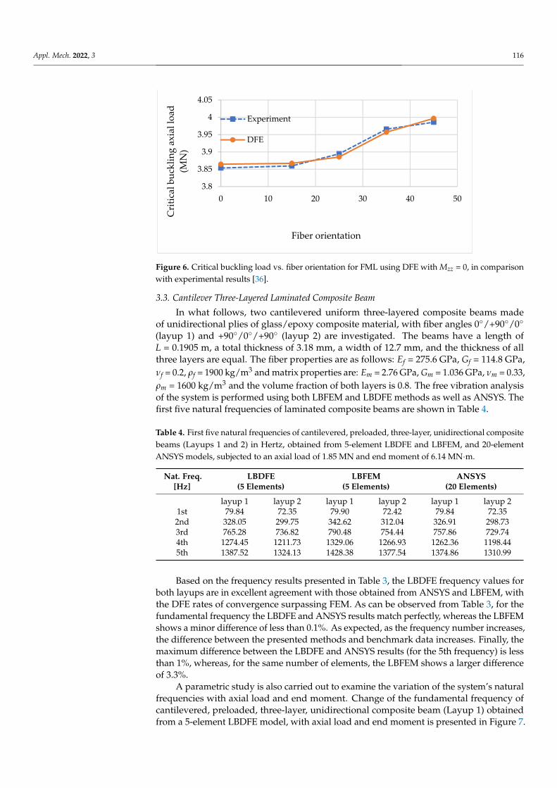
It is possible to use the modal analysis to find critical axial force or critical end mo-ment causing buckling by keeping one of them constant and increasing the other one until the fundamental frequency vanishes, i.e., zero stiffness, or static (structural) instability, which means structural failure. The result of this analysis is presented in Figure 5. As the end moment increases, the structure becomes less rigid which requires a lower axial force to buckle. To validate the results of DFE buckling analysis, in Figure 6 a comparison is presented between experimental study [36] and DFE results for different fiber orientations with Mzz = 0.

00.20.40.60.8

11.21.41.6

0 2 4 6 8 10 12

Rela

tive

erro

r (%

)

Number of elements

DFE FEM

00.20.40.60.8

11.21.41.61.8

0 10 20 30 40 50 60Fund

amen

tal f

requ

ency

(HZ)

Axial force (KN)

M=0 M=26.2KN.m M=52.5KN.m

Figure 3. The convergence study for the two proposed LBFEM and LBDFE formulations; relativeerror of fundamental frequency for cantilevered FML three-layer beam subjected to an axial load of17.5 MN and end moment of 52.5 KN·m.

Appl. Mech. 2022, 3 115

Appl. Mech. 2022, 3 114

a factor of five. An analysis is also carried out to investigate the effects of both axial force and end moment (combined) on the fundamental frequencies of the beam. Figure 4 illus-trates the variation of the first natural frequency with tensile axial force and end moment using the DFE method.

Figure 3. The convergence study for the two proposed LBFEM and LBDFE formulations; relative error of fundamental frequency for cantilevered FML three-layer beam subjected to an axial load of 17.5 MN and end moment of 52.5 KN·m.

Figure 4. Fundamental frequency vs. tensile force and end moment for the cantilevered three-layer FML beam.

It is possible to use the modal analysis to find critical axial force or critical end mo-ment causing buckling by keeping one of them constant and increasing the other one until the fundamental frequency vanishes, i.e., zero stiffness, or static (structural) instability, which means structural failure. The result of this analysis is presented in Figure 5. As the end moment increases, the structure becomes less rigid which requires a lower axial force to buckle. To validate the results of DFE buckling analysis, in Figure 6 a comparison is presented between experimental study [36] and DFE results for different fiber orientations with Mzz = 0.

00.20.40.60.8

11.21.41.6

0 2 4 6 8 10 12

Rela

tive

erro

r (%

)

Number of elements

DFE FEM

00.20.40.60.8

11.21.41.61.8

0 10 20 30 40 50 60Fund

amen

tal f

requ

ency

(HZ)

Axial force (KN)

M=0 M=26.2KN.m M=52.5KN.m

Figure 4. Fundamental frequency vs. tensile force and end moment for the cantilevered three-layerFML beam.

It is possible to use the modal analysis to find critical axial force or critical end momentcausing buckling by keeping one of them constant and increasing the other one until thefundamental frequency vanishes, i.e., zero stiffness, or static (structural) instability, whichmeans structural failure. The result of this analysis is presented in Figure 5. As the endmoment increases, the structure becomes less rigid which requires a lower axial forceto buckle. To validate the results of DFE buckling analysis, in Figure 6 a comparison ispresented between experimental study [36] and DFE results for different fiber orientationswith Mzz = 0.

Appl. Mech. 2022, 3 115

Figure 5. Buckling analysis for three-layer FML cantilevered beam using 5-element DFE.

Figure 6. Critical buckling load vs. fiber orientation for FML using DFE with Mzz = 0, in comparison with experimental results [36].

3.3. Cantilever Three-Layered Laminated Composite Beam In what follows, two cantilevered uniform three-layered composite beams made of

unidirectional plies of glass/epoxy composite material, with fiber angles 0°/+90°/0° (layup 1) and +90°/0°/+90° (layup 2) are investigated. The beams have a length of L = 0.1905 m, a total thickness of 3.18 mm, a width of 12.7 mm, and the thickness of all three layers are equal. The fiber properties are as follows: Ef = 275.6 GPa, Gf = 114.8 GPa, νf = 0.2, ρf = 1900 Kg/m3 and matrix properties are: Em = 2.76 GPa, Gm = 1.036 GPa, νm = 0.33, ρm = 1600 Kg/m3 and the volume fraction of both layers is 0.8. The free vibration analysis of the system is performed using both LBFEM and LBDFE methods as well as ANSYS. The first five nat-ural frequencies of laminated composite beams are shown in Table 4.

0

5

10

15

20

25

30

35

-2 -1 0 1 2 3

Buck

ling

Mom

ent (

MN

.m)

Axial force (MN)

3.8

3.85

3.9

3.95

4

4.05

0 10 20 30 40 50

Cri

tical

buc

klin

g ax

ial l

oad

(MN

)

Fiber orientation

Experiment

DFE

Figure 5. Buckling analysis for three-layer FML cantilevered beam using 5-element DFE.

Appl. Mech. 2022, 3 116

Appl. Mech. 2022, 3 115

Figure 5. Buckling analysis for three-layer FML cantilevered beam using 5-element DFE.

Figure 6. Critical buckling load vs. fiber orientation for FML using DFE with Mzz = 0, in comparison with experimental results [36].

3.3. Cantilever Three-Layered Laminated Composite Beam In what follows, two cantilevered uniform three-layered composite beams made of

unidirectional plies of glass/epoxy composite material, with fiber angles 0°/+90°/0° (layup 1) and +90°/0°/+90° (layup 2) are investigated. The beams have a length of L = 0.1905 m, a total thickness of 3.18 mm, a width of 12.7 mm, and the thickness of all three layers are equal. The fiber properties are as follows: Ef = 275.6 GPa, Gf = 114.8 GPa, νf = 0.2, ρf = 1900 Kg/m3 and matrix properties are: Em = 2.76 GPa, Gm = 1.036 GPa, νm = 0.33, ρm = 1600 Kg/m3 and the volume fraction of both layers is 0.8. The free vibration analysis of the system is performed using both LBFEM and LBDFE methods as well as ANSYS. The first five nat-ural frequencies of laminated composite beams are shown in Table 4.

0

5

10

15

20

25

30

35

-2 -1 0 1 2 3

Buck

ling

Mom

ent (

MN

.m)

Axial force (MN)

3.8

3.85

3.9

3.95

4

4.05

0 10 20 30 40 50

Cri

tical

buc

klin

g ax

ial l

oad

(MN

)

Fiber orientation

Experiment

DFE

Figure 6. Critical buckling load vs. fiber orientation for FML using DFE with Mzz = 0, in comparisonwith experimental results [36].

3.3. Cantilever Three-Layered Laminated Composite Beam

In what follows, two cantilevered uniform three-layered composite beams madeof unidirectional plies of glass/epoxy composite material, with fiber angles 0◦/+90◦/0◦

(layup 1) and +90◦/0◦/+90◦ (layup 2) are investigated. The beams have a length ofL = 0.1905 m, a total thickness of 3.18 mm, a width of 12.7 mm, and the thickness of allthree layers are equal. The fiber properties are as follows: Ef = 275.6 GPa, Gf = 114.8 GPa,νf = 0.2, ρf = 1900 kg/m3 and matrix properties are: Em = 2.76 GPa, Gm = 1.036 GPa, νm = 0.33,ρm = 1600 kg/m3 and the volume fraction of both layers is 0.8. The free vibration analysisof the system is performed using both LBFEM and LBDFE methods as well as ANSYS. Thefirst five natural frequencies of laminated composite beams are shown in Table 4.

Table 4. First five natural frequencies of cantilevered, preloaded, three-layer, unidirectional compositebeams (Layups 1 and 2) in Hertz, obtained from 5-element LBDFE and LBFEM, and 20-elementANSYS models, subjected to an axial load of 1.85 MN and end moment of 6.14 MN·m.

Nat. Freq.[Hz]

LBDFE(5 Elements)

LBFEM(5 Elements)

ANSYS(20 Elements)

layup 1 layup 2 layup 1 layup 2 layup 1 layup 21st 79.84 72.35 79.90 72.42 79.84 72.352nd 328.05 299.75 342.62 312.04 326.91 298.733rd 765.28 736.82 790.48 754.44 757.86 729.744th 1274.45 1211.73 1329.06 1266.93 1262.36 1198.445th 1387.52 1324.13 1428.38 1377.54 1374.86 1310.99

Based on the frequency results presented in Table 3, the LBDFE frequency values forboth layups are in excellent agreement with those obtained from ANSYS and LBFEM, withthe DFE rates of convergence surpassing FEM. As can be observed from Table 3, for thefundamental frequency the LBDFE and ANSYS results match perfectly, whereas the LBFEMshows a minor difference of less than 0.1%. As expected, as the frequency number increases,the difference between the presented methods and benchmark data increases. Finally, themaximum difference between the LBDFE and ANSYS results (for the 5th frequency) is lessthan 1%, whereas, for the same number of elements, the LBFEM shows a larger differenceof 3.3%.

A parametric study is also carried out to examine the variation of the system’s naturalfrequencies with axial load and end moment. Change of the fundamental frequency ofcantilevered, preloaded, three-layer, unidirectional composite beam (Layup 1) obtainedfrom a 5-element LBDFE model, with axial load and end moment is presented in Figure 7.

Appl. Mech. 2022, 3 117

As can be observed, when the axial force is increased, the natural frequency decreases.However, as the end moment is increased, the system’s frequency decreases.

Appl. Mech. 2022, 3 116

Table 4. First five natural frequencies of cantilevered, preloaded, three-layer, unidirectional compo-site beams (Layups 1 and 2) in Hertz, obtained from 5-element LBDFE and LBFEM, and 20-element ANSYS models, subjected to an axial load of 1.85 MN and end moment of 6.14 MN·m.

Nat. Freq. [Hz] LBDFE (5 Elements)

LBFEM (5 Elements)

ANSYS (20 Elements)

layup 1 layup 2 layup 1 layup 2 layup 1 layup 2 1st 79.84 72.35 79.90 72.42 79.84 72.35 2nd 328.05 299.75 342.62 312.04 326.91 298.73 3rd 765.28 736.82 790.48 754.44 757.86 729.74 4th 1274.45 1211.73 1329.06 1266.93 1262.36 1198.44 5th 1387.52 1324.13 1428.38 1377.54 1374.86 1310.99

Based on the frequency results presented in Table 3, the LBDFE frequency values for both layups are in excellent agreement with those obtained from ANSYS and LBFEM, with the DFE rates of convergence surpassing FEM. As can be observed from Table 3, for the fundamental frequency the LBDFE and ANSYS results match perfectly, whereas the LBFEM shows a minor difference of less than 0.1%. As expected, as the frequency number increases, the difference between the presented methods and benchmark data increases. Finally, the maximum difference between the LBDFE and ANSYS results (for the 5th fre-quency) is less than 1%, whereas, for the same number of elements, the LBFEM shows a larger difference of 3.3%.

A parametric study is also carried out to examine the variation of the system’s natural frequencies with axial load and end moment. Change of the fundamental frequency of cantilevered, preloaded, three-layer, unidirectional composite beam (Layup1) obtained from a 5-element LBDFE model, with axial load and end moment is presented in Figure 7. As can be observed, when the axial force is increased, the natural frequency decreases. However, as the end moment is increased, the system’s frequency decreases.

Figure 7. Fundamental frequency of cantilevered, preloaded, three-layer, unidirectional composite beam (Layup 1) obtained from a 5-element LBDFE model, subjected to various axial loads and end moments.

Figures 8 and 9, respectively, show bending and torsional components of the first five mode shapes of the cantilevered, preloaded, three-layer, unidirectional composite beam (Layup1) obtained using a 20-element LBDFE model, subjected to an axial load of 1.85 MN and end moment of 6.14 MN·m. The horizontal axis represents the normalized dis-tance from the fixed end of the beam (x/L). As can be seen from the figures, the first three and fifth modes are predominantly bending with a slight influence of torsion, whereas the third mode has a predominant torsional character.

0

20

40

60

80

100

120

0 0.5 1 1.5 2Fund

amen

tal F

requ

ency

(Hz)

Axial Force (MN)

M=0 M=6.14MN.m M=9.21MN.m

Figure 7. Fundamental frequency of cantilevered, preloaded, three-layer, unidirectional compositebeam (Layup 1) obtained from a 5-element LBDFE model, subjected to various axial loads and endmoments.

Figures 8 and 9, respectively, show bending and torsional components of the first fivemode shapes of the cantilevered, preloaded, three-layer, unidirectional composite beam(Layup 1) obtained using a 20-element LBDFE model, subjected to an axial load of 1.85 MNand end moment of 6.14 MN·m. The horizontal axis represents the normalized distancefrom the fixed end of the beam (x/L). As can be seen from the figures, the first three andfifth modes are predominantly bending with a slight influence of torsion, whereas the thirdmode has a predominant torsional character.

Appl. Mech. 2022, 3 117

Figure 8. Bending component of the first five mode shapes of the cantilevered, preloaded, three-layer, unidirectional composite beam (Layup1) obtained using a 20-element LBDFE model, sub-jected to an axial load of 1.85 MN and end moment of 6.14 MN·m.

Figure 9. Torsion component of the first five mode shapes of the cantilevered, preloaded, three-layer, unidirectional composite beam (Layup1) obtained using a 20-element LBDFE model, sub-jected to an axial load of 1.85 MN and end moment of 6.14 MN·m. 4. Discussion

The free vibration analysis of Fiber-Metal Laminated (FML) and unidirectional com-posite beams subjected to axial force and end moment is presented using layered Finite Element Method (FEM) and Dynamic Finite Element (DFE) models. The frequency results are compared with those obtained from the conventional FEM (ANSYS) as well as the homogenization technique. Based on the results shown in Table 1, the presented layered FEM method has higher a rate of convergence compared to the method of homogenization while DFE has a higher rate of convergence compared to the FEM method, which makes DFE the most efficient method. Considering the benchmark, the estimated error of the FML beam fundamental frequency for the DFE method using five elements along the beam length is almost zero. This error for the layered FEM method using five elements, is around 0.64% while for the method of homogenization using the same number of

Figure 8. Bending component of the first five mode shapes of the cantilevered, preloaded, three-layer,unidirectional composite beam (Layup 1) obtained using a 20-element LBDFE model, subjected to anaxial load of 1.85 MN and end moment of 6.14 MN·m.

Appl. Mech. 2022, 3 118

Appl. Mech. 2022, 3 117

Figure 8. Bending component of the first five mode shapes of the cantilevered, preloaded, three-layer, unidirectional composite beam (Layup1) obtained using a 20-element LBDFE model, sub-jected to an axial load of 1.85 MN and end moment of 6.14 MN·m.

Figure 9. Torsion component of the first five mode shapes of the cantilevered, preloaded, three-layer, unidirectional composite beam (Layup1) obtained using a 20-element LBDFE model, sub-jected to an axial load of 1.85 MN and end moment of 6.14 MN·m. 4. Discussion

The free vibration analysis of Fiber-Metal Laminated (FML) and unidirectional com-posite beams subjected to axial force and end moment is presented using layered Finite Element Method (FEM) and Dynamic Finite Element (DFE) models. The frequency results are compared with those obtained from the conventional FEM (ANSYS) as well as the homogenization technique. Based on the results shown in Table 1, the presented layered FEM method has higher a rate of convergence compared to the method of homogenization while DFE has a higher rate of convergence compared to the FEM method, which makes DFE the most efficient method. Considering the benchmark, the estimated error of the FML beam fundamental frequency for the DFE method using five elements along the beam length is almost zero. This error for the layered FEM method using five elements, is around 0.64% while for the method of homogenization using the same number of

Figure 9. Torsion component of the first five mode shapes of the cantilevered, preloaded, three-layer,unidirectional composite beam (Layup 1) obtained using a 20-element LBDFE model, subjected to anaxial load of 1.85 MN and end moment of 6.14 MN·m.

4. Discussion

The free vibration analysis of Fiber-Metal Laminated (FML) and unidirectional com-posite beams subjected to axial force and end moment is presented using layered FiniteElement Method (FEM) and Dynamic Finite Element (DFE) models. The frequency resultsare compared with those obtained from the conventional FEM (ANSYS) as well as thehomogenization technique. Based on the results shown in Table 1, the presented layeredFEM method has higher a rate of convergence compared to the method of homogenizationwhile DFE has a higher rate of convergence compared to the FEM method, which makesDFE the most efficient method. Considering the benchmark, the estimated error of theFML beam fundamental frequency for the DFE method using five elements along the beamlength is almost zero. This error for the layered FEM method using five elements, is around0.64% while for the method of homogenization using the same number of longitudinalelements it is 2.24%. As expected, and with reference to Figures 3 and 6 (three-layer unidi-rectional glass/epoxy composite beam, layup 1), the tensile axial load increases the naturalfrequencies of the beam, indicating an increase in the stiffness of the beam. When theend moment is increased, the natural frequencies reduce, indicating a reduction in thestiffness of the beam. If the end moment is held constant and the tensile load is increased,the natural frequencies increase indicating an increase in the beam stiffness. Conversely,if the tensile load is held constant and the end moment is increased, the beam stiffnessreduces. Considering Figures 7 and 8, the coupled vibration of the beam is found to bepredominantly flexural in the first few natural frequencies (the first three, for the casestudied here) and torsion becomes predominant at a higher natural frequency starting fromthe fourth mode.

In summary, in all cases studied in this paper, the convergence rates obtained fromfrequency-dependent Dynamic Finite Element (DFE) formulation are found to surpass thosefound from the conventional FEM, which in turn surpass the method of homogenization.The higher convergence rate of DFE is mainly attributed to the usage of the solutions to theuncoupled part of equations as the basis functions of approximation space. In comparisonwith conventional FEM, which uses simple polynomial shape functions, the interpolationfunctions derived from these solutions provide much better approximations for elementdisplacements expressed in terms of nodal displacements. This higher rate of convergencemeans that in order to reach a specific accuracy, DFE requires a much smaller number ofelements than FEM. This might not look like a huge advantage in the analysis of simple

Appl. Mech. 2022, 3 119

structures like the ones studied here but in large–scale designs of complex systems usingDFE would lead to much less computation time.

It is also worth mentioning that the developed conventional and dynamic FEMs herehave advantages over FEM based software, ANSYS in modeling prestressed beams, sincehere the axial force and end moment are included in the equations of motion. Therefore,the developed FEMs give the natural frequency and mode shapes of vibration directly. Touse the modal analysis in ANSYS for a prestressed structure, however, one needs to firstsolve the problem statically. Then, the results of static analysis are to be used to find thenew stiffness of the prestressed structure, which will be used later in modal mode to findnatural frequencies.

In this study, the effect of interlayer slip was not considered. So, as a proposed futurework, the interlayer slip can be added to the DFE model of layered beams subjected to axialforce and end moment.

Author Contributions: This paper presents the results of a recent research, conducted by M.K.under the supervision of S.M.H. All authors have read and agreed to the published version of themanuscript.

Funding: This research was funded by a Discovery Grant from Natural Sciences and EngineeringResearch Council of Canada (NSERC), RGPIN-2017-06868.

Data Availability Statement: All data generated or analyzed during this study are included withinthe article.

Acknowledgments: Supports provided by National Sciences and Engineering Research Councilof Canada (NSERC), Ontario Graduate Scholarship (OGS) program, and Ryerson University, areacknowledged.

Conflicts of Interest: The authors declare no conflict of interest.

References1. Neogy, J.; Murthy, M.K.S. Determination of fundamental natural frequencies of axially loaded columns and frames. J. Inst. Eng.

1969, 49, 203–212.2. Prasad, K.S.R.K.; Krishnamurthy, A.; Mahabaliraja, A.V. Iterative type Rayleigh-Ritz method for natural vibration. Am. Inst.

Aeronaut. Astronaut. J. 1970, 8, 1884–1886. [CrossRef]3. Timoshenko, S. Vibration Problems in Engineering; Van Nostrand: Opelika, AL, USA, 1964.4. Williams, F.W.; Banerjee, J.R. Flexural vibration of axially loaded beams with linear or parabolic taper. J. Sound Vib. 1985, 99,

121–138. [CrossRef]5. SHashemi, M.; Richard, J.M. Free Vibration Analysis of Axially Loaded Bending-Torsion Coupled Beams—A Dynamic Finite

Element (DFE). Comput. Struct. 2000, 77, 711–724. [CrossRef]6. Banerjee, J.R. Explicit modal analysis of axially loaded composite Timoshenko beams using symbolic computation. J. Aircr. 2002,

39, 909–912. [CrossRef]7. Hashemi, S.M.; Roach, A. Dynamic Finite Element Analysis of Extensional-Torsional Coupled Vibration in Nonuniform Composite

Beams. Appl. Compos. Mater. 2011, 18, 521–538. [CrossRef]8. Gellert, M.; Gluck, J. The influence of axial load on eigenfrequencies of a vibrating lateral restraint cantilever. Int. J. Mech. Sci.

1972, 14, 723–728. [CrossRef]9. Tarnai, T. Variational methods for analysis of lateral buckling of beams hung at both ends. Int. J. Mech. Sci. 1979, 21, 329–335.

[CrossRef]10. Banerjee, J.R.; Williams, F.W. Coupled bending—Torsional dynamic stiffness matrix of an axially loaded Timoshenko beam

element. Int. J. Solids Struct. 1994, 31, 749–762. [CrossRef]11. Leung, A.Y.T. Natural shape functions of a compressed Vlasov element. Thin-Walled Struct. 1991, 11, 431–438. [CrossRef]12. Joshi, B.; Suryanarayan, S. Coupled flexural—Torsional vibration of beams in the presence of static axial loads and end moments.

J. Sound Vib. 1984, 92, 583–589. [CrossRef]13. Joshi, A.; Suryanarayan, S. Unified Analytical Solution for Various Boundary Conditions for the Coupled Flexural-torsional

Vibration of Beams Subjected to Axial Loads and End Moments. J. Sound Vib. 1989, 129, 313–326. [CrossRef]14. Joshi, A.; Suryanarayan, S. Iterative method for coupled flexural–torsional vibration of initially stressed beams. J. Sound Vib. 1991,

146, 81–92. [CrossRef]15. Williams, F.W.; Kennedy, D. Exact dynamic member stiffnesses for a beam on an elastic foundation. Earthq. Eng. Struct. Dyn.

1987, 15, 133–136. [CrossRef]

Appl. Mech. 2022, 3 120

16. Issa, M.S. Natural frequencies of continuous curved beams on Winkler-type foundation. J. Sound Vib. 1988, 127, 291–301.[CrossRef]

17. Mei, C. Coupled vibrations of thin-walled beams of open section using the finite element method. Int. J. Mech. Sci. 1970, 12,883–891. [CrossRef]

18. Banerjee, J.R.; Fisher, S.A. Coupled bending-torsional dynamic stiffness matrix for axially loaded beam elements. Int. J. Numer.Methods Eng. 1992, 33, 739–751. [CrossRef]

19. Hashemi, S.M. Free-Vibrational Analysis of Rotating Beam-Like Structures: A Dynamic Finite Element Approach. Ph.D. Thesis,Department of Mechanical Engineering, Laval University, Quebec, QC, Canada, 1998.

20. Hasim, K.A. Isogeometric static analysis of laminated composite plane beams by using refined zigzag theory. Compos. Struct.2018, 186, 365–374. [CrossRef]

21. Kefal, A.; Hasim, K.A.; Yildiz, M. A novel isogeometric beam element based on mixed form of refined zigzag theory for thicksandwich and multilayered composite beams. Compos. Part B Eng. 2019, 167, 100–121. [CrossRef]

22. Foraboschi, P. Analytical Solution of Two-Layer Beam Taking into Account Nonlinear Interlayer Slip. J. Eng. Mech. 2009, 135,124–139. [CrossRef]

23. Cas, B.; Planinc, I.; Schnabl, S. Analytical solution of three-dimensional two-layer composite beam with interlayer slips. Eng. Struct.2018, 173, 269–282. [CrossRef]

24. Cortés, F.; Sarría, I. Dynamic Analysis of Three-Layer Sandwich Beams with Thick Viscoelastic Damping Core for Finite ElementApplications. Shock Vib. 2015, 2015, 736256. [CrossRef]

25. Ross, D.; Kerwin, E.M.; Ungar, E.E. Damping of plate flexural vibration by means of viscoelastic laminae. In Structural Damping,Section II; ASME: New York, NY, USA, 1959.

26. Mohri, F.; Azrar, L.; Potier-Ferry, M. Vibration analysis of buckled thin-walled beams with open sections. J. Sound Vib. 2004, 275,434–446. [CrossRef]

27. Franzoni, F.; de Almeida, S.F.M.; Ferreira, C.A.E. Numerical and Experimental Dynamic Analyses of a Postbuckled Box Beam.AIAA J. 2016, 54, 1987–2003. [CrossRef]

28. Augello, R.; Daneshkhah, E.; Xu, X.; Carrera, E. Efficient CUF-based method for the vibrations of thin-walled open cross-sectionbeams under compression. J. Sound Vib. 2021, 510, 116232. [CrossRef]

29. Kashani, M.T.T.; Jayasinghe, S.; Hashemi, S.M. On the flexural-torsional vibration and stability of beams subjected to axial loadand end moment. Shock Vib. 2014, 2014, 153532. [CrossRef]

30. Kashani, M.T.; Jayasinghe, S.; Hashemi, S.M. Dynamic Finite Element Analysis of Bending-Torsion Coupled Beams Subjected toCombined Axial Load and End Moment. Shock Vib. 2015, 2015, 471270. [CrossRef]

31. Kashani, M.T.; Hashemi, S.M. On the Free Vibration Analysis of Prestressed Fiber-Metal Laminated Beam Elements. In Proceedingsof the 15th International Conference on Civil, Structural and Environmental Engineering Computing, Prague, Czech Republic, 1–4 September2015; Kruis, J., Tsompanakis, Y., Topping, B.H.V., Eds.; Civil-Comp Press: Stirlingshire, UK, 2015; p. 107. [CrossRef]

32. ANSYS, Inc. ANSYS® Academic Research, Release 13.0, Help System, Coupled Field Analysis Guide; ANSYS Inc.: Canonsburg, PA,USA, 2010.

33. Bathe, K.-J. Finite Element Procedures in Engineering Analysis; Prentice Hall: Hoboken, NJ, USA, 1982.34. Wittrick, W.H.; Williams, F.W. A General Algorithm for Computing Natural Frequencies of Elastic Structures. Q. J. Mech. Appl.

Math. 1971, 24, 263–284. [CrossRef]35. Banerjee, J.R.; Cheung, C.W.; Morishima, R.; Perera, M.; Njuguna, J. Free vibration of a three-layered sandwich beam using the

dynamic stiffness method and experiment. Int. J. Solids Struct. 2007, 44, 7543–7563. [CrossRef]36. Plantema, F. Sandwich Construction: The Bending and Buckling of Sandwich Beams, Plates, and Shells; Wiley: New York, NY, USA,

1966.