EPR DOSIMETRY WITH TOOTH ENAMEL: A REVIEW

1

EPR DOSIMETRY WITH TOOTH ENAMEL: A REVIEW.

Paola Fattibene1* and Freddy Callens2

1Istituto Superiore di Sanità, Department of Technology and Health, Viale Regina Elena

299, I-00161 Rome, Italy. [email protected]

2Ghent University, Department of Solid State Sciences, Krijgslaan 281-S1, B-9000

Gent, Belgium. [email protected]

*Corresponding author:

Paola Fattibene

Istituto Superiore di Sanità, Department of Technology and Health

Viale Regina Elena 299

I-00161 Rome, Italy

Tel. +39 06 499092248

[email protected]

Met opmaak: Engels

(Groot-Brittannië)

2

Abstract

When tooth enamel is exposed to ionizing radiation, radicals are formed that can be

detected using Electron Paramagnetic Resonance (EPR) techniques. EPR dosimetry

using tooth enamel is based on the (presumed) correlation between the intensity or

amplitude of some of the radiation-induced signals with the dose absorbed in the

enamel. In the present paper a critical review is given of this widely applied dosimetric

method.

The first part of the paper is quite fundamental and deals with the main properties of

tooth enamel and several of its model systems (e.g., synthetic apatites). Considerable

attention is also devoted to the numerous radiation-induced and native EPR signals, and

the radicals responsible for them. The relevant EPR detection, identification and

spectrum analysing methods are reviewed from a general point of view. Finally, the

need for solid state modelling and the linearity of the dose response are investigated.

The second part is devoted to the practical implementation of EPR dosimetry using

enamel. It concerns the preparation of samples, specific irradiation problems, spectrum

acquisition and it is described how the dosimetric signal intensity and dose can be

retrieved from the EPR spectra. Special attention is paid to the energy dependence of

the EPR response and to sources of uncertainties. Results of and problems encountered

in international intercomparisons and epidemiological studies are also dealt with.

In the final chapter the future of EPR dosimetry with tooth enamel is analysed.

Keywords:

EPR, ESR, tooth enamel, dosimetry

3

1. Introduction

Electron paramagnetic resonance, EPR, (or alternatively, electron spin resonance, ESR)

spectroscopy is the only method to detect, identify, and quantify free radicals (Halliwell

and Gutteridge, 2007; Punchard and Kelly, 1996). EPR quantitation of the radiation-

induced radicals makes it possible to measure the radiation dose absorbed by the

irradiated material. Due to this ability, EPR dosimetry has developed into one of the

most widely used and recognized applications in the universe of EPR (Lund and

Shiotani, 2003). It has been used in industrial irradiations, medicine, environmental

sciences, geology, and archaeology. Established applications of EPR dosimetry are

control of radiation processing (ISO, 2004), identification of irradiated foods (CEN,

1996; CEN, 2000; CEN, 2001), evaluation of radiation risk (ICRU, 2002), and dating

(Ikeya, 1993). Efforts are being made to use it in radiation oncology (Mathias, 2006).

The purpose of this paper is to review the available literature on the EPR dosimetry

using tooth enamel. Several reviews have been published over the period of the

technique development from its inception to the present state of relative maturity.

However, most of these reviews either covered only selected aspects of the method

(Pass, 1997; Bhat, 2005), or were limited in size (Desrosiers and Schauer, 2001;

Romanyukha and Regulla, 1996; Regulla, 2005; Romanyukha et al., 2000a), or were

focused on the comparison of EPR dosimetry with other dosimetric techniques (Straume

et al., 1997; Kleinerman et al., 2006). In 2002, an extensive report prepared by a group

of authors was published by IAEA (IAEA, 2002). Our review is coming out about seven

years later.

2. A short history of EPR dosimetry using tooth enamel

The first EPR detection of radiation-induced radicals in calcified tissues dates back to

1955, when Gordy et al. (1955) reported the EPR spectrum of an x-ray-irradiated skull

bone recorded at 9 and 23 GHz. A few years later, in 1963, Cole and Silver reported the

first observation of several radiation-induced EPR signals in human teeth (Cole and

Silver, 1963). The authors recorded a spectrum of a fraction of an in vitro x-ray-

4

irradiated deciduous incisor at 24 GHz and concluded that at least three types of

paramagnetic species appeared to occur in the tissue. Using tooth enamel as a dosimeter

when man-made dosimeters are not available was suggested for the first time by Brady

et al. (1968), who reported a minimum detectable dose below 1 Gy and a linear dose

response. It was clear since then that tooth enamel was a suitable material for individual

dosimetry, but the criticism based on the obvious problem of sample collection has been

a limit to its practical use for years.

The evolution of the scientific activity around tooth enamel dosimetry can be seen

from: (i) the growing popularity of the ESR Dosimetry Conference; (ii) the rapid growth

of the number of publications in this field, and (iii) the history of international

intercomparisons. This deserves to be discussed in somewhat greater detail.

(i) For about 15 years after the publication of the milestone paper by Brady et al.

(1968) mentioned above, tooth enamel dosimetry has been oriented mostly towards

dating applications. In 1985, the First International Symposium on ESR Dating, held at

Ube-Akiyoshi (Japan), included dosimetry: a few papers presented there described

application of EPR of tooth enamel to reconstruction of doses received by people

exposed to the explosions of the atomic bombs. After that, the interest in tooth enamel

dosimetry has been increasing at the subsequent conferences of this series (Table 1), and

the conference focus has gradually shifted from dating dosimetry to retrospective

dosimetry. The 1998, 2006 and 2008 meetings were joint conferences on EPR dating

and biodosimetry. Furthermore, since the late 1990’s, tooth dosimetry has also been a

topic at other conferences, namely, the International Conference on Solid State

Dosimetry and the International Conference on Luminescence and Electron Spin

Resonance Dating (McKeever, 2000; Horowitz and Oster, 2002; d'Errico and

McKeever, 2006; Bos, 2008).

(ii) Fig. 1 shows the trend in the number of publications in the area of tooth dosimetry

in the Journal of Citation Report (JCR) between 1986 and 2008 (search performed in

October of 2009 for keywords “tooth enamel” and “dosimetry”). A positive trend with

time is clearly seen, with a leap by a factor of about two in 1996. After that, there have

been a minimum of 11 and a maximum of 30 publications per year. This rise in the JCR

publication rate around 1996 can be explained by the increased interest of public

funding organizations in the use of tooth dosimetry as a tool for dose reconstruction in

5

epidemiological cohorts, mainly in the studies of health effects of radiation on the

Chernobyl liquidators in Ukraine, the populations of the Southern Urals in Russia, and

the residents near the Semipalatinsk Nuclear Test Site in Kazakhstan (Chumak et al.,

1997; Haskell, 1997; Gusev et al., 1997; Ivannikov et al., 1997; Romanyukha et al.,

1996a; Vorobiova et al., 1999; Wieser et al., 2000a).

(iii) Four international intercomparisons have been arranged since 1994 to check the

consistency of the doses assessed by different laboratories. The results of these

intercomparisons will be described in a later chapter of this review. It is worth noting

the number of the participating institutions: (1st) 1994-1995, 9 participants (Chumak et

al., 1996a); (2nd) 1999, 18 participants (Wieser et al., 2000b; Wieser et al., 2000c); (3rd)

2003-2004, 14 participants (Wieser et al., 2005; Wieser et al., 2006a); (4th) 2006, 10

participants (Hoshi et al., 2007; Ivannikov et al., 2007). While writing this review,

another intercomparison has started involving 16 participating laboratories. The first

intercomparison had not been announced in the scientific community, which explains

why the number of its participants was twice as small as the number of the participants

in the second intercomparison. Later, a few laboratories abandoned the technique and

even fewer laboratories adopted it. A core group of eight laboratories participated in the

latest three intercomparisons. In other words, the method has not spread much beyond

the initial scientific community. An obvious reason for this is the cost of the

instrumentation, but the need for expertise in both radiation dosimetry and EPR may be

also a disincentive.

An analysis of these indicators shows that EPR tooth dosimetry has reached a level

of 18 publications per year on average since 1996. The most productive period was

probably between 1999 and 2002, which also saw publication of two important

international reports (IAEA, 2002; ICRU, 2002). The large number of publications in

the last few years demonstrates still high activity, which was probably stimulated by a

couple of lively international conferences.

It is also interesting to note how the application field of tooth dosimetry has changed

with time. In the early years, the method was proposed for dose assessments when no

other dosimetry estimates were available, as is the case of radiation accidents involving

general population. At that time, the recurring question was whether tooth dosimetry

was more suitable for retrospective dosimetry than the other biodosimetry techniques.

6

As the method evolved and its advantages and weaknesses got understood better, it

became clear that tooth dosimetry is more appropriate as a reference method for

validation of other dose assessment techniques. At present, the question is not which

method is better, but rather how the ensemble of the existing retrospective dosimetry

methods can be used jointly for accurate assessment of doses (ICRU, 2002).

The aforementioned facts of the still fairly restricted use of the method, the apparent

plateau stage in its development and, at the same time, the sufficiently high degree of its

establishment have motivated us to write this review. It seems that the due time has

come to assemble the available data and to try to create a coherent picture of the method

with all its advantages and limitations. We have written this paper for the community of

specialists in EPR retrospective dosimetry in an attempt to provide them with a

comprehensive review of the published literature. We have written it also for scientists

with expertise only in EPR or only in retrospective dosimetry in order to equip them

with knowledge that would help them understand this field and, hopefully, find it

attractive.

3. Tooth anatomy and morphogenesis

3.1. Human dentition

Man has two dentitions: the primary one, which is fully erupted approximately at the

age of two, and the permanent one, which replaces the primary dentition when the

person is between six and thirteen years old. Deciduous incisors, canines and molars are

eventually all replaced by their respective permanent counterparts. Moreover,

permanent dentition has 12 additional molars. Consequently, there are 20 deciduous and

32 permanent teeth.

The notation most widely used to indicate a specific tooth in a mouth is the one

recommended by ISO (ISO, 1984); it was proposed by the International Dental

Federation (FDI) and approved by the World Health Organization (WHO). According to

this standard system, a tooth is designated by a code composed of two numbers, which

indicate, respectively, the quadrant (labelled clockwise from the right side of the

7

maxilla1) and the tooth position in the quadrant (labelled from the front to the back). For

example, a tooth designated as 1.1 is the first incisor of the right quadrant of the

maxilla.

The visible part of the tooth is called crown, while the part covered by the gum is

called root. The bulk of the tooth is composed of dentin, which is surrounded by a thin

layer of enamel in the tooth crown and by a thin layer of cementum in the root.

Internally, dentin contains pulp, which is the only noncalcified tooth tissue; it hosts

blood vessels and nerves. The tooth is anchored to the jaw bone by the root. The four

vertical sides of a tooth are called lingual, buccal, mesial, and distal. The surface of

tooth facing the tongue is called lingual, while the opposite side is called buccal (labial

for incisors). Mesial and distal are the other two sides, the former being the side closer

to the front part of the oral cavity.

This text is intended to provide basic information necessary for using tooth enamel

dosimetry. Therefore, attention will be focused mainly on morphogenesis and histology

of tooth enamel. Description of dentin and cementum will be restricted to the aspects

significant for dose reconstruction. The reader can learn more from the book edited by

Chadwick and Cardew (1997).

3.2. The tooth enamel

3.2.1. Tooth enamel histology

The histological structure of tooth enamel is formed by mineral crystallites of

hydroxyapatite grouped in clusters with hexagonal cross-sections (called prisms or

rods). These clusters are bound together by interprismatic (sometimes called interrod)

enamel, which also consists of hydroxyapatite crystallites, but these crystallites are

oriented in a direction different from that in the prisms. The rods are 1-2 nm thick, 5-10

nm deep and 1 mm long (the latter number corresponds approximately to the full

thickness of the enamel in a tooth) (Martin et al., 1988). The rods begin at the junction

between dentin and enamel (dentin-enamel junction) and grow more or less

perpendicular to it. For several reasons, the crystals do not grow uninterruptedly parallel

1 Maxilla and mandible are the upper and lower jaw major bones, respectively,

8

to each other and perpendicular to the surface, but show discontinuities in orientation

(Boyde et al., 1988).

3.2.2. Tooth enamel morphogenesis

Enamel mineral is initially formed at the dentin-enamel junction. When the crystals

have nucleated2 (by a process that is not completely understood), they elongate in the

direction perpendicular to the junction (defined as the crystal c-axis) to form the

aforementioned rods.

Cells that secrete enamel crystals are called ameloblasts; they are derived from the

embryonic ectoderm3. Ameloblast is a unique highly-polarized protein cell that secretes

extracellular protein matrix involved in production and mineralization of enamel. This

extracellular protein matrix is formed by two types of proteins, amelogenins and non-

amelogenins. The amelogenin component constitutes approximately 80% of the total

protein matrix during the enamel development phase.

Formation of apatite crystals has three stages: secretion, transition and maturation.

� Secretion stage. Formation and growth of the crystals are possible due to

continuous supply of calcium. Most probably, this is provided by an active

calcium pump, which transfers calcium ions out of ameloblast cells (Sasaki et

al., 1990; Takano, 1995). This process creates a high local concentration of

calcium, which results in precipitation of calcium phosphate in the vicinity of

the cells. In the framework of this model, each prism corresponds to a single

ameloblast, while the interprismatic enamel corresponds to intercellular sites. At

this stage, ameloblasts secrete amelogenins. Fig. 2 shows a model proposed for

the mechanism by which amelogenins control the size, morphology and

orientation of the crystallites. According to this model, amelogenins self-

assemble into quasi-spherical structures (nanospheres) approximately 20 nm in

2 Nucleation is the first stage of mineral formation. It is a chain of events that leads to a stable cluster of ions capable of surviving and growing. 3 The embryo is formed by three primary layers, which are, from the outermost to the innermost, the ectoderm, the mesoderm and the endoderm, each giving rise to different body tissues. The epidermis and associated tissues (nails, hair, tooth enamel and cementum) originate from the ectoderm, whereas the bone (skeletal, cartilage, tooth dentine) originates from the mesoderm. This partly explains why enamel is different from bones and dentine.

9

diameter, which are deposited around and between the developing mineral

ribbons. They act as scaffolding and prevent lateral mineral accretion and

crystal-crystal fusion, but leave the c-axial crystal surface exposed to calcium

and phosphate ions (Fincham and Simmer, 1997).

� Transition stage. Ameloblast cells start to reduce in height; matrix secretion

ceases, and proteins are withdrawn. The concentration of the protein component,

which was 20-30% at the early stage of amelogenesis, gradually decreases in the

process of enamel mineralization.

� Maturation stage. At this stage, the formation of the bulk of enamel is

completed. The enamel crystals grow significantly in width and thickness until

most of the tissue volume is occluded with the mineral. The crystal growth

requires elimination of the protein matrix. It has been postulated that enzymes

(serine proteases) degrade amelogenins to small fragments in order to facilitate

their removal at the maturation stage. The gradual loss of enamel proteins is

accompanied by an increase of the amount of materials of smaller molecular

weight. The breakdown products undergo resorption by secretory ameloblasts.

Residual breakdown products and proteins constitute only approximately 1% of

the weight of adult enamel.

Thus, tooth formation is a complex process, which takes years to be fully

completed. In this process, the tooth enamel transforms from a cellular tissue rich of

functional proteins (at the secretory stage, when it is also called enamel organ) into a

fully mineralized tissue containing only functional residual breakdown products and

proteins. Table 2 shows the chronology of tooth development. The time of the first

evidence of calcification corresponds to the beginning of the secretion stage, whereas

the time of the enamel completion is the end of the maturation stage.

3.2.3. The mineral phase

As mentioned above, the mineral component of enamel is hydroxyapatite. Apatites are a

family of compounds characterized by a similar structure, albeit with different

compositions. Most of the current knowledge about the enamel apatite has been derived

from studies of related synthetic or natural compounds.

10

Normally, hydroxyapatite crystallizes in the monoclinic space group P21/b (a =

0.94214 nm, b = 2a, and c = 0.68814 nm). The crystallographic structure of

hydroxyapatite, as it occurs in biological apatites, is hexagonal with space group P63/m

and lattice parameters a = b = 0.9432 nm and c = 0.6881 nm (Bres et al., 1993). The

unit-cell of the apatite crystal contains 10 +2Ca , 6 −3

4PO and 2 −OH ions. The −3

4PO

ions are packed hexagonally, which produces channels. The −OH ions are positioned in

columns along these channels, and each −OH ion (e.g., z = ¼ and z = ¾ in c units) is

surrounded by three +2Ca ions at the same height in a configuration with a 120°

symmetry. The two “Ca2+ triangles” are shifted by 60°. Each of these six Ca2+ ions has

an accompanying 3

4PO − group with the P nucleus at z = ¼ for the Ca2+ ion located at z =

¾ and vice versa (Ca-II ions). At a longer distance, one finds six Ca-I ions in a similar

pseudo-hexagonal arrangement. The subtle difference between the hexagonal and

monoclinic structure is in the ordering of the hydroxyl groups. We refer the reader to

the more specialized literature for a detailed discussion (see, e.g., Driessens and

Verbeeck, 1990; Elliot, 1969; Elliot et al., 1973).

Biological apatites contain also 2-3% of −2

3CO ions. Carbonate can be present as an

adsorbed phase, or as a lattice substituent, or both (Le Geros, 1981; Elliot, 1994). As a

lattice component, it can substitute for either −3

4PO (B-site substitution) or −OH (A-site

substitution). In the former case, a −2

3CO ion replaces a single −3

4PO ion, while, in the

latter case, a −2

3CO ion substitutes for two −OH ions. In either case, the substitution

induces variations in the crystal lattice parameters a and c because the O-O distance in

−2

3CO is different from the O-H distance in −OH and the O-O distance in −3

4PO . The

model of the substitution of phosphate with carbonate implies that the planar carbonate

molecule lies in parallel with one of the inclined faces formerly occupied by the −3

4PO

tetrahedron. Substitution of phosphate by carbonate involves a reorganization of ions

and vacancies (Fig. 3). Approximately 11% of the −2

3CO ions are located in the c-axis

channels and substitute for −OH ions (Elliot et al., 1985).

11

Minor constituents and trace elements get incorporated in tooth enamel during

mineralization (Tables 3 and 4). There is some variation in the compositions reported in

the literature (LeGeros, 1981; Priest and Van De Vyver, 1990). Trace elements and

minor constituents may play a role in the stability of apatite, in the inhibition or

promotion of calcification, and in the susceptibility of the mineral to dissolution in

acids. The concentrations of these elements change from the external surface to the

dentin-enamel junction. Some elements may change the lattice parameters significantly

even when present in low concentrations (LeGeros, 1981). It has been hypothesized that

paramagnetic impurities are responsible for parasitic signals in the EPR spectrum of

tooth enamel (Shishkina et al., 2001b). Doi et al. (1981b), who studied EPR spectra of

heated calcified tissues, suggested that such signals are produced by trivalent chromium,

probably associated with organic constituents.

Water is present on the surface of enamel as an absorbate and in the enamel crystal

lattice. Adsorbed water has no effect on the lattice parameters of hydroxyapatite and can

be completely eliminated by heating to temperatures above 200 °C. Lattice water is a

result of substitution of H2O for OH-, of HPO42- for PO4

3-, and of HCO3- for CO3. It

becomes thermally unstable between 200 and 400 °C and affects crystal lattice

parameters.

3.2.4. The protein phase

The hydroxyapatite content of mature enamel is 96% by weight and 85% by volume.

The rest is protein (1%) and water (3%). In the process of enamel development, the

protein content decreases from 20% (by weight) at the secretory stage down to 1% in

the end of the maturation stage (Deutsch and Alayoff, 1987). The residual breakdown

products and proteins present at the end of the maturation stage are rich of proline,

glycine and glutamic acid. It was initially believed that the protein in mature enamel

was either keratin, like in other ectodermic tissues (nails, dermas, hair), or collagen, like

in dentine and bone. These two hypotheses were abandoned when proline was found in

the enamel protein phase, because neither collagen, nor keratin contains it (Fawcett and

Jensh, 2002).

3.3. Tooth dentine and cementum

12

Dentin is the substance that makes up the bulk of the tooth. It is harder than bone, but

softer than enamel. About 70% of dentin is mineral matter.

Histologically, dentin consists of a calcified matrix with dentinal tubules. The latter

are minute canals containing tiny projections of the odontoblasts (the dentin-forming

cell). These cells are not inside dentin, but in a layer on the wall of the pulp cavity. The

odontoblast projections are protoplasmic processes called fibers of Tomes. They

connect dentin with odontoblasts, which, in turn, are connected with the nerves in the

dental pulp. It is due to these processes that dentine is sensitive to external stimuli like

heat, cold, or touch. Generally, the dentinal tubules follow a somewhat S-shaped

course, beginning at the surface of the pulp and ending at the junction with enamel.

Some of the dentinal tubules go through the dentino-enamel junction and terminate in

the enamel.

The calcified matrix is made of hydroxyapatite crystallites, which are much smaller

(approximately 5 × 30 × 100 nm3) and more randomly oriented than crystallites in

enamel, and contains about 4-5% of carbonate. The higher concentration of carbonate

and other impurities in comparison with enamel is believed to be the reason for the

lower crystallinity in dentine (Le Geros, 1981).

The protein component of dentine consists mainly of Type I collagen and, to a lesser

extent, of non-collagenous proteins. The former is organized in a lattice to assist

formation of carbonate apatite, and the latter are likely to control initiation and growth

of the crystals. The organic component of dentin is very similar to that of bone, except

that dentine also contains a few unique proteins (dentine phosphophoryn, dentine matrix

protein 1 and dentine sialoprotein).

Dentin of a newly-formed tooth is called primary dentin. In the course of life, new

portions of dentin are continuously formed with a parallel progressive shrinking of the

pulp area. This process is due mostly not to primary dentin, whose growth is very slow,

but to another dentinal tissue, called regular secondary dentin. This secondary dentin is

produced on the walls of the pulp cavity, and its growth can even completely fill the

cavity if the production is very effective. Nonetheless, the volume of secondary dentin

is always much smaller than the volume of the primary dentin. Growth of secondary

dentin is more pronounced in the root than in the crown.

13

Finally, there is a third type of dentin. When dental pulp is irritated as a result of

caries, abrasion, or erosion, new dentin, called reparative, or irregular secondary, dentin,

is formed at the site of the structural change. Thus, formation of dentin is a complex and

non-uniform process, which continues throughout the whole life of the tooth.

Cementum is a thin layer of calcified connective tissue that covers tooth roots.

Approximately 55% of cementum is inorganic matter (primarily calcium salts), and the

rest is organic compounds (mainly collagen). Histologically, there are two types of

cementum: cell-free (primary) and cellular (secondary). Primary cementum is

distributed fairly uniformly over the surface of the root, whereas cellular cementum

contains cells similar to those of bone and is usually confined to the apical root.

Microscopic images of cementum show light and dark concentric rings (Renz et al.,

1997), and some authors have tried to correlate the number of these rings with the tooth

age (Stott et al., 1982).

So, in comparison with enamel, dentin and cementum contain less mineral material,

and ordering of their microcrystals is poorer, which may be the reason for the lower

radiation sensitivities of their EPR responses. The continuous formation of new portions

of dentin and cementum precludes long-term storage of the radiation damage, which

makes these materials unreliable dose recorders. For this reason, the EPR responses of

dentine and cementum to radiation have been scarcely investigated, although they could

be valuable in comparing doses assessed in the same tooth by the three different tissues.

3.4. Primary teeth

“Primary teeth” is the clinically accurate term for the temporary dentition, although

several other names are commonly used (deciduous, baby, milk or first teeth). The

development stages of primary teeth are shown in Table 2, too. Calcification begins in

the fourth month of foetal life. By the time when the primary teeth have fully erupted

(around the second year of the child’s life), the crowns of permanent teeth have started

to calcify.

The root of a primary tooth is completely formed about one year after the tooth

eruption, but it is short-lived. Three years later, resorption of the root begins. Complete

resorption of the roots of primary teeth makes their exfoliation and replacement by

permanent teeth possible.

14

Primary teeth are usually smaller than permanent ones, have much thinner enamel

and dentin, and a much larger pulp chamber. As a consequence, their crowns appear

whiter in color. The ordering of the crystallites is probably poorer in milk teeth than in

permanent ones (Skaleric et al., 1982). Primary and mature enamels are similar in terms

of amino acid composition, except the latter contains more glycine (Wright et al., 1997).

There are few studies of the radiation response of the EPR signal of primary teeth

(Haskell et al., 1999a; Wieser and El-Faramaway, 2002; El-Faramaway and Wieser,

2006; Section 20.4).

3.5. Carious teeth

Most of the teeth available for EPR examination are carious or diseased. Under normal

conditions, tooth enamel is protected against attacks of the acids in the metabolism of

sugars, thanks to the carbonate and phosphate buffers of saliva. Tooth caries is a result

of demineralization of enamel, which is induced when the production of buffers is

slower than the production of acids. In such case, acids diffuse in enamel (diffusion

coefficient 10-8 cm2 s-1) and can penetrate into the tissue for a depth of a few hundred

microns (Driessens and Verbeeck, 1990). Some constituents of enamel can increase or

decrease the diffusion coefficient. Of particular interest for tooth dosimetry is the

known correlation of the vulnerability of enamel to acid with the carbonate/phosphate

concentration ratio in the tooth (Sobel, 1962). For this reason, carbonate has been called

“Achilles heel” of enamel (Hardwick, 1949). Aoba et al. (1982) found the 3

3

O

CO

−

−

concentration ratio to be higher for carious than for sound teeth. However, there is no

evidence of a difference between carious and healthy parts of teeth in terms of the

radiation sensitivity of their EPR responses (Sholom et al., 2000b). Among the

impurities, incorporated strontium, which substitutes for calcium, has been found to

reduce carbonate incorporation in apatite, thus affecting the acid diffusion coefficient

(Driessens and Verbeeck, 1990, p. 266-267; Le Geros, 1981). Based on EPR

measurements, some authors associated the resistance to caries with the degree of

microcrystal alignment in enamel prisms (Cevc et al., 1976). However, this hypothesis

has not been supported by results of other investigators (Martens et al., 1986; Gualtieri

et al., 1999).

15

3.6. Nonhuman dentition

Some authors have recently proposed to use animal teeth for dose reconstruction, as will

be discussed in Section 20.5. It should be borne in mind, however, that animals vary

widely in terms of dentition morphology and anatomy. Moreover, even teeth in different

positions in the mouth of the same animal may vary significantly in morphology.

Sufficient knowledge in these areas is necessary not only for performing experiments

with animals, but also for interpreting available data.

Within the class of mammals, the main differentiation is between low-crowned, or

brachidont, and high-crowned, or ipsodont, teeth. The former is the type described

above for humans; it can be found in all the carnivor and omnivor animals. The latter

type is characterized by continuous growth during the tooth lifetime. This is possible

because the external part of the tooth consists not entirely of enamel, but also of

secondary dentine and cementum. This type of dentition is typical of herbivors. The

crown of such a tooth is longer than the crown of a brachidont, and it is partly covered

by gum. Such teeth are being worn off during the tooth life, but the continuous growth

partially compensates for this wear, and the tooth volume changes with the age of the

animal. The saying "never look into the mouth of a gift horse” originates from the

common practice to estimate age of horses by evaluating the size of their teeth.

4. Theoretical introduction to EPR

4.1. General introduction to spectroscopy

EPR is a non-destructive spectroscopic technique used to detect and/or identify

paramagnetic systems. The latter are characterized by the presence of at least one

unpaired electron and can be atoms, molecules, molecular ions, etc. An important

category (and the only one relevant to EPR dosimetry using tooth enamel) are radicals

in solids, characterized by one unpaired electron. When a paramagnetic system is

placed in a magnetic field, its energy levels split (Zeeman splitting). Radicals have two

low-lying Zeeman levels corresponding to the ground state (Fig. 4).

Spectroscopy in general involves measurement and interpretation of energy

differences, the knowledge of which gives insight into the identity, microscopic

16

structure and dynamics of the system under study. These energy differences ∆E can be

measured because, as can be shown in quantum mechanics, electromagnetic radiation

incident on a sample will be absorbed if

∆ = νE h , (4.1)

where h is Planck’s constant and ν is the frequency of the radiation. The quantity hν is,

then, the energy of the incident radiation (photon or quantum). The absorption of

energy results in a transition of the system from the lower energy state to the higher

energy state.

In conventional spectroscopy, the frequency ν is varied (swept), and, at certain

values corresponding to ∆E in Eq. (4.1), absorption peaks will occur, giving rise to what

is called an (absorption) spectrum. A wide range of frequencies can be used to perform

different types of spectroscopy (e.g., IR, UV, NMR spectroscopy). In EPR

experiments, microwave radiation (ν in the gigahertz range, 109 s-1) is used. We will

now confine ourselves to EPR and discuss the Zeeman effect mentioned above in

somewhat more detail.

4.2. Principles of EPR

Atomic or molecular systems with unpaired electrons have a magnetic moment µ�

,

which behaves like a compass needle or a bar magnet when put into a magnetic field.

The energy differences ∆E used in EPR are due to the interaction of this magnetic

moment with the magnetic field �B . According to classical physics, the state with the

lowest energy corresponds to µ�

parallel to �B , whereas the energy for µ

� anti-parallel to

�B is highest (Fig. 5).

Mathematically, this interaction energy can be expressed by the following scalar, or

inner, product:

.= −µ��

potE B . (4.2)

According to quantum mechanics, however, the magnetic moment will not be aligned as

in Fig. 5, but will make a finite angle with the direction of the magnetic field vector (z)

and precess around it. For a system with one unpaired electron, the projection of the

magnetic moment on the z-axis is “quantized” and can only have two distinct values

(corresponding to the classical parallel and anti-parallel orientations in Fig. 5). These

17

two states are called eigenstates of the system and labelled as |MS> = |-1/2> ≡ |β> and

|MS> = |1/2> ≡ |α>, respectively. This is typical for an electron spin S = ½. For a

general spin S, the spin quantum number MS may have values -S, -S+1, …, S-1, and S

(that is, there are 2S+1 possibilities corresponding to 2S+1 Zeeman levels).

Consequently, for S = 1/2, there are only two Zeeman levels. The magnetic moment µ�

is characteristic for each paramagnetic system. It consists of two fundamental

contributions, which, in a somewhat simplified picture, can be seen as arising from the

rotation of the electrons about their own axes and from the orbital motion of the

electrons around the nuclei. Whereas the former (intrinsic spin) is the same for all

electrons, the latter depends on the specific atom or molecule and the (crystalline)

environment in which it is located. It is this contribution that determines the g factor (or

simply g) and makes it possible to discriminate between paramagnetic systems. The g-

factor expresses the proportionality between the electron spin (angular moment) and the

magnetic moment (the minus sign is due to the negative charge of the electron):

g Sµ = − β��

. (4.3)

The Bohr magneton, β (also often denoted Bµ ), is the natural unit of magnetic moment.

In order to get some feeling of the origin of Eq. (4.3), the reader should consult any

textbook on classical physics (e.g., Halliday, Resnick and Walker, 2004, pp. 871-873),

where the relation between the orbital angular momentum �L and the magnetic moment

µ�

is discussed.

The factor g can range widely (variations between 1 and 3 are not exceptional), but,

in the simplest case, g = ge = 2.0023 (this is the free electron value, without orbital

contribution). For most molecules, g will be close to this value (see Section 4.3 and

examples in the next chapter).

Combining Eqs. (4.2) and (4.3) yields the following expression for the potential

energy of a free electron in a magnetic field �B :

( ). ( )= + β = β + + = β��

pot e e x x y y z z e z zE g B S g B S B S B S g B S , (4.4)

when the z-axis is advantageously chosen along the direction of the applied magnetic

field.

In quantum mechanics, the energy is quantized, and the only allowed energies (in fact,

the eigenvalues of the spin Hamiltonian operator ˆβe zg BS ) are

Met opmaak: Engels(Groot-Brittannië)

Met opmaak: Engels(Groot-Brittannië), Spelling engrammatica controleren

Met opmaak: Engels

(Groot-Brittannië)

Met opmaak: Engels

(Groot-Brittannië), Spelling engrammatica controleren


Met opmaak: Engels

(Groot-Brittannië)



Met opmaak: Engels(Groot-Brittannië), Spelling en

grammatica controleren

Met opmaak: Engels








Verwijderd: (4.3)

Verwijderd: (4.2)

Verwijderd: (4.3)

18

E(MS) = ( , 1,..., 1, )β = − − + −e S Sg BM M S S S S . (4.5)

For one unpaired electron, S equals 1/2, and this leads to

1 1

( )2 2

+ = βeE g B (the “spin up” state denoted by |MS> = |1/2> ≡ |α>, the

highest energy corresponding to the magnetic moment anti-parallel to the magnetic

field) (4.6)

and

1 1

( )2 2

− = − βeE g B (the “spin down” state denoted by |MS> = |-1/2> ≡ |β>, the

lowest energy corresponding to the magnetic moment parallel to the magnetic field). (4.7)

In an EPR experiment, a different way of obtaining spectra is used than in most

other spectroscopies: instead of varying the (microwave) frequency, one varies the

magnetic field B at a fixed frequency ν, and the two energy levels, E(+1/2) and E(-1/2),

get split proportionally to B. Resonance will take place when the energy of the applied

microwave radiation, hν, matches the difference between the two levels (Fig. 4 and Eq.

(4.1)):

1 1

( ) ( )2 2

ν = ∆ = + − − = βeh E E E g B , (4.8)

leading to the resonance field for a free electron

ν

=β

res

e

hB

g. (4.9)

Moreover, it is usually the first derivative of the absorption with respect to the magnetic

field, dy/dB, rather than absorption itself, what is detected in EPR spectroscopy (Fig. 4).

The most common line shapes will be discussed in more detail in Chapter 5.

For an unpaired electron in a free atom or ion (i. e., in the absence of neighbors

like ions in a crystal lattice to interact with) exhibiting full rotational symmetry,

ν

=β

res

L

hB

g. (4.10)

The quantity gL is called the Landé factor. A closed formula can be derived for it

(Atherton, 1993, pp. 36-46), and, depending on the specific electron configuration of the

atom or ion, it can deviate from ge significantly. It can be, for example, (approximately)

1 or 3.5.

Met opmaak: Engels

(Groot-Brittannië)

Met opmaak: Engels





Verwijderd: (4.1)

19

For any system without anisotropy, we can generalize:

ν

=β

res

hB

g, (4.11)

where g is called simply the “g-factor” or “g-value”.

One should be aware that the resonance field is not a unique “fingerprint” of a

paramagnetic system because it depends on the used microwave frequency. The true

“fingerprint” is the g-value or the g-tensor, as will be further explained below. The

frequencies and microwave bands commonly used in EPR will be discussed in Chapters

5 and 6.

In anisotropic systems, like an unpaired electron in a (free) molecule or in an

atom/ion in a crystal lattice, the relation between magnetic and angular momenta

becomes more complicated, and so do the equations involved (T means transposing the

matrix):

( ... ) [ ] [ ][ ] . .= β + + + = β ≡ β�� T

pot x xx x x xy y z zz zE B g S B g S B g S B g S B g S . (4.12)

Thus, in anisotropic systems, a 3 × 3 g-matrix [g] or tensor g�

has to be used instead of a

single g-value. When the x, y and z-axes are chosen properly (i.e., the so-called

principal axes are selected, or “g-tensor is diagonalized”), the g-matrix becomes much

simpler: it contains only three non-zero elements residing on its diagonal (the so-called

principal g-values). Like any second-rank tensor (or symmetrical 3 × 3 matrix), the g-

tensor has only 6 independent quantities, namely, the three principal values, gx, gy and

gz, and three parameters that determine the three orthogonal principal axes of the tensor.

The principal axes may be, for example, symmetry axes in a molecule (see examples

below).

Accordingly, in the principal axes frame, Eq. (4.12) becomes considerably

simpler:

( ) ( )= β + + = β + +pot x x x y y y z z z x x y y z zE g B S g B S g B S B g lS g mS g nS . (4.13)

Here, l, m and n are the direction cosines of B�

in the principal axes system.

These special directions x, y and z are imposed by (the symmetry of) the system and

cannot be chosen arbitrarily (except of a permutation of x, y and z, although z is usually

chosen along the main symmetry axis of the system).

Verwijderd: (4.12)

20

Expression (4.13) is fully symmetric in x, y and z, and it can be easily

understood that applying the magnetic field consecutively in the direction of each of the

three principal axes will yield gx, gy and gz. For example,

ν

=β

y

y

hg

B, (4.14)

where By is the resonance field measured at �B parallel to the gy principal axis.

Experiments of this kind can only be performed if a highly-ordered system, such as a

single crystal, is available.

By calculating the eigenvalues of the operator corresponding to Eq. (4.13), one

can derive for S = 1/2:

2 2 2 2 2 21 1( )

2 2± = ± + + βx y zE g l g m g n B (4.15)

(cf. Eqs. (4.6) and (4.7)).

This means that, for an arbitrary orientation (l, m, n) of the magnetic field,

2 2 2 2 2 2x y zg g l g m g n= + + , (4.16)

i. e., the g-value changes when the system is rotated in the magnetic field.

This equation implies that one of the principal values corresponds to the highest

possible g-value (gmax), whereas another one is the lowest possible (gmin). These two g-

values determine the boundaries of the EPR spectrum, i.e., max

ν

β

h

g and

min

ν

β

h

g, when a

full orientational study is performed or when a powder spectrum is recorded. These

limits will be extended somewhat by the line width and, possibly, by hyperfine

interactions (see below).

Before dealing with the information contained in the principal g-values, we will

shortly discuss a phenomenon called “saturation”, which sometimes occurs in EPR.

Instead of considering just an individual electron as was done above, we now need to

consider all unpaired electrons of all atoms in interaction with the environment. In

principle, the EPR signal grows in intensity with increasing microwave power, which is

related to the number of microwave photons hν incident on the sample per unit time and

per unit area. It is essential for this increase that considerably more electrons reside at

the lowest Zeeman level (MS = -1/2) than at the higher level(s), in line with Fermi or

Boltzmann statistics. This poses no problems as long as the energy of the incident










Met opmaak: Engels

(Groot-Brittannië)



Verwijderd: (4.13)

Verwijderd: (4.13)

Verwijderd: (4.6)

Verwijderd: (4.7)

21

microwave radiation can be effectively dissipated via the coupling between the spin

system and the surrounding lattice (spin-lattice relaxation). This mechanism may

become less efficient at high microwave powers and/or low temperatures, leading to a

zero or very small difference between the populations of the Zeeman levels. This

means that no or only a very weak net absorption will be detected. When such

saturation occurs, the EPR signal may be deformed, decreased in magnitude or even

completely suppressed. Therefore, such circumstances should be avoided, unless for

specific purposes (e.g., ENDOR). In practice, this can be checked by plotting the EPR

signal height versus the square root of the microwave power, which should yield a

straight line in the absence of saturation.

4.3. Information contained in the principal g-values

g-Tensor is characteristic for a paramagnetic system and is determined by two factors.

In the first place, it is determined by the central atom or molecule containing the

unpaired electron (free system). In the second place, it is affected by its (nearest)

environment, mainly the host lattice and its defects and impurities. With a certain

model for the paramagnetic system, the principal values can be calculated either

analytically (e.g., by perturbation methods, as described in the books by Abragam and

Bleaney, 1970, pp. 277 – 345, and Atherton, 1993, pp. 130-168) or numerically, using,

for example, density functional theory (DFT) methods (Lund and Shiotani, 2003, pp.

267-302). Details of such techniques are beyond the scope of this paper, but, typically,

expressions like the following can be derived for the gi (Lund and Shiotani, 2003, pp.

267-302):

1 2

1 2

...λ λ

= ± ± ±∆ ∆

a bi eg g n n

E E (i = x, y, z). (4.17)

Here, the λ values are spin-orbit coupling constants for atoms a, b, etc., making up the

molecule, and the ∆E values are splittings between the ground state and certain excited

states. The ni values are small integers. A more adequate, but more complicated

formula of this type applicable to many molecules has been derived by Stone (1963).

Thus, the principal g-values contain some information about the electronic structure of

the paramagnetic species.

22

When the excited states have substantially higher energies than the ground state

(∆E >> λ), as is the case for most molecules, all principal g-values will be close to ge

(reflecting a negligible orbital contribution to the electron magnetic moment). This will

make it more difficult to differentiate between them.

It is the symmetry of the system that largely imposes the orientation of the

principal axes and determines whether or not two or all three principal g-values are

equal. If a system has axial symmetry (e.g., a free diatomic molecule like superoxide

2O− ), the g-tensor will be axial, i.e., ⊥= ≡x yg g g and =�zg g . As will be discussed in

greater detail below, the equality of certain principal g-values can give important

information about the symmetry and geometric structure of the involved radicals.

4.4. Hyperfine Interactions

Although the g-tensor contains information about the electronic structure of

paramagnetic species, which makes it possible to differentiate between them, it, by

itself, is often not sufficient for identification. Fortunately, unpaired electrons are quite

sensitive to the environment. When the magnetic moment µ�

of the unpaired electron

“feels” the presence of another magnetic moment of a nucleus, an extra contribution

appears in the expression for the energy, which is called the hyperfine (HF)

contribution:

, . . [ ] [ ][ ] ...= ≡ = + + +� � �

Tpot HF x xx x x xy y z zz zE S A I S A I S A I S A I S A I . (4.18)

A magnetic nucleus has a non-zero nuclear spin I, resulted from the way of pairing of its

protons and neutrons. 1H, 13C, 31P (all have I = 1/2) and 17O (I = 5/2) are the most

relevant isotopes in the context of this review. (The reader should be aware that the

most relevant nuclei in tooth enamel, namely, 12C and 16O, have zero spins). The extra

energy in Eq. (4.18) can be understood classically as follows. The magnetic moment of

a nearby nucleus induces a local magnetic field �BI at the electron, which has to be

added to, or subtracted from, the external magnetic field �B , depending on the

orientation of the moment of the nucleus. According to quantum mechanics, there are,

again, two possible orientations for a nuclear spin of 1/2, resulting in two resonance

fields and, thus, a splitting of the EPR signal into two hyperfine lines (Fig. 6).

Met opmaak: Engels

(Groot-Brittannië)

Met opmaak: Engels




Met opmaak: Engels

(Groot-Brittannië)

Verwijderd: (4.18)

23

Accordingly, each of these lines is (approximately) at a distance of BI from the

original position given by Eq. (4.11). It can be deduced from Eq. (4.2) that the

interaction energy between two magnetic dipoles is

3( . )( . ) . 3( . )( . ) .0 0( ) ( ), 5 3 5 34 4

ˆ ˆ[ ] [ ][ ] . .

µ µµ µ µ µ= − − = β β −

π π

= ≡

� ��

� � �

r r S r I r S II IE g gpot HF e N Nr r r r

TS T I S T I

(4.19)

(This can be found in many physics textbooks, too.) The magnetic moment µ = β��

I N Ng I

is associated with the nuclear angular moment �I . In these equations, βN and gN are the

nuclear counterparts of electron’s β and g, and µ0 is the permeability of the vacuum.

The vector �r describes the position of the unpaired electron spin with respect to the

nucleus. The reason why we have replaced the ‘A’ symbol in Eq. (4.18) with ‘T’ to

indicate the hyperfine interaction will be clarified below, but it is essentially a result of a

partial failure of the classical theory.

When the nucleus is far enough from the unpaired electron (typically

approximately 0.4 nm or more away), the latter can be considered as localized at one

point (point dipole approximation). We can now use Eq. (4.19) to derive expressions

for the principal values of the T-tensor (matrix):

03

0// 3

1;

4

2.

4

x y e N N

z e N N

T T T g gr

T T g gr

⊥

µ= ≡ = − ββ

π

µ≡ = ββ

π .

(4.20)

These values can be found on the diagonal of the matrix if the z-axis is chosen along the

line connecting the electron and the nucleus (x = 0, y = 0, z = r for the “point electron”).

Notice that these couplings decrease quickly with the increasing distance to the nucleus

(~3

1

r) and that Tx + Ty + Tz = 0. If the values of T⊥ and T� can be determined

experimentally, we can calculate the electron–nucleus distance and the direction in

which the nucleus is located (direction of maximal T = T� ). This procedure was applied

in a few ENDOR studies (see the following chapters and references therein).

A more rigorous treatment reveals that, due to the presence of s-electrons, an

extra term, so-called Fermi-contact term,






Met opmaak: Engels

(Groot-Brittannië)






Met opmaak: Engels

(Groot-Brittannië)

Verwijderd: (4.11)

Verwijderd: (4.2)

Verwijderd: (4.19)

24

202| (0) |

3

µ= β β ψiso e N NA g g (4.21)

has to be added to the three principal values Tx, Ty and Tz found above. In this

expression, 2| (0) |ψ is the probability of finding the electron at the nucleus, which is

non-zero only for s-electrons.

In general, the magnetic hyperfine interaction is a sum of both dipolar (T’s) and

contact (Aiso) contributions, and the hyperfine term in our expression for the energy can

be written in the form:

, . . .( ).= = +� � ��

pot HF isoE S A I S A T I . (4.22)

As the sum of all principal T’s is zero, it follows that

( ) ( ) ( ) 3+ + = + + + + + =x y z iso x iso y iso z isoA A A A T A T A T A , (4.23)

from which Aiso and the T values can be simply derived.

This procedure of finding the T values necessary for calculating distances to

neighboring nuclei (using Eq. (4.20)) works well only when all the principal g-values

are close to ge (which is, fortunately, largely the case in all the systems of our interest).

It will be discussed elsewhere how the principal A-values can be determined. We refer

the reader to the specialized literature for a description of more accurate treatments of

the hyperfine interaction (e.g., Atherton, 1993, pp.169-223). As is the case for the g-

tensor, high-level first-principles calculations of hyperfine couplings are perfectly

feasible nowadays, using, e.g., DFT (Lund and Shiotani, 2003, pp. 239-265). However,

for several radicals relevant to the present paper (CO2-, CO3

3-), GAMESS90, CNDO/II

and INDO calculations were quite successfully performed already fifteen years ago (see,

e.g., Moens et al., 1994b,c). Finally, it is worth mentioning that the term

“superhyperfine interaction” is used to emphasize that the unpaired electron interacts

with nuclei outside of the central defect or radical.

4.5. Consequences of the hyperfine interaction for the EPR spectrum

When there is an interacting nucleus with a non-zero nuclear spin I, the |MS>

eigenfunctions of the electron Zeeman Hamiltonian ˆβe zg BS represented in Eq. (4.4) do

not describe the paramagnetic system accurately, and the nuclear spin state has to be

specified. In the first-order approximation, which is sufficient for our purposes, the

Met opmaak: Engels

(Groot-Brittannië)

Met opmaak: Engels








Met opmaak: Engels



Verwijderd: (4.20)

Verwijderd: (4.4)

25

eigenvalues (energies) of the spin Hamiltonian extended to cover hyperfine interactions

are

( ) = β +S I S S IE M M g BM AM M (4.24)

with

2 2 2 2 2 2 2 2 2

2

2

+ +=

x x y y z zA g l A g m A g nA

g (cf. Eq. (4.16)). (4.25)

The states |MI> (MI = -I, -I + 1, …, I – 1, and I) are eigenfunctions of the ˆzI operator

similar to the eigenfunctions |MS> are for the operator ˆzS . By analogy with the

definitions made in Eqs. (4.6) and (4.7), for I = ½, we have the “nuclear spin up” and

“nuclear spin down” states. Thus, for systems with one unpaired electron (S = ½)

interacting with either 1H, 13C or 31P (I = ½), there are four states |MS >|MI>, i. e.

(2S+1)(2I+1) energy levels instead of the two discussed in Section 4.2 (|1/2 1/2>, |1/2 -

1/2>, |-1/2 1/2>, |-1/2 -1/2>). Taking into account the quantum mechanical selection

rules |∆MS | = 1 and ∆MI = 0 (flip of the electron spin, no flip of the nuclear spin), two

allowed EPR transitions instead of one arise at magnetic fields (to the first order):

12

ν ν= + = +

β β βI

h A hB B

g g g (|-1/2 -1/2> → |+1/2 -1/2>) (4.26)

and

22

ν ν= − = −

β β βI

h A hB B

g g g (|-1/2 +1/2> → |+1/2 +1/2>). (4.27)

This explains the spectrum shown in Fig. 6 from a quantum-mechanical viewpoint.

For a general nucleus, this becomes

( )ν

= +β β

II

AMhB M

g g (to the first order and for the 2I+1 possible values of MI). (4.28)

As an example of an I = 5/2 system, the frequently observed six-line (2I + 1 = 6)

spectrum of Mn2+ is shown in Fig. 7. The magnetic field corresponding to ge is between

the third and the fourth lines.

It may be noteworthy that A has the dimension of energy (like hν) and that the

lines represented by Eqs. (4.26) and (4.27) are apart by the value β

A

g (= 2BI defined

above). The latter, of course, has the dimension of magnetic field induction and is




Met opmaak: Engels

(Groot-Brittannië)

Met opmaak: Engels








Met opmaak: Engels

(Groot-Brittannië)

Verwijderd: (4.16)

Verwijderd: (4.6)

Verwijderd: (4.7)

26

independent of the microwave frequency used in the EPR experiment! The lines are

placed symmetrically around the resonance field 0

ν=

β

hB

g, where a single resonance

line would have been found in the absence of the nuclear spin. The quantity β

A

g is

often denoted by A’ and expressed in tesla or gauss (1 T = 104 G). Hyperfine values are

also frequently expressed in MHz. The conversion involves Planck’s constant h, and

the relationship between A’ (T) and A (MHz) is

4( ) 2.80247 10 '( )=e

gA MHz x A T

g. (4.29)

5. EPR spectra of single crystals and powders

5.1. Introduction

An EPR spectrum is characterized by the g- and A-tensors (in many cases,

simply the g- and A-values) and the line shape. The vast majority of the EPR spectra

used in tooth dosimetry are spectra of powders. A powder is characterized by a random

distribution of the individual crystallites, so that its spectrum is the envelope of the

spectra of small single crystals oriented in all possible directions with respect to the

magnetic field. If the single-crystal spectrum of a certain defect does not change upon

rotation, the powder spectrum will be, in principle, identical to it. Therefore, a good

strategy for gaining insight into the spectra of powders is to start the discussion with the

single-crystal spectra of paramagnetic systems of different symmetries (isotropic, axial

and orthorhombic). We will confine ourselves to static systems (no movements) with

one unpaired electron (S = ½) and without hyperfine interactions. Before a discussion

of the relation between single-crystal and powder spectra in Section 5.3, we will provide

a brief introduction to the basics of EPR line widths.

5.2. EPR spectrum line shape

The line shape of an EPR signal is a very complicated matter. It may be affected

by so-called homogeneous and inhomogeneous broadening. Homogeneous broadening

27

can be properly described only in terms of quantum mechanics. According to the

Heisenberg uncertainty principle, it is related to the lifetimes of the energy levels

involved in the transitions. These lifetimes are determined by the energy exchange

between the unpaired electrons (spin system) on the one hand and the environment

(lattice) on the other, or simply between the spins themselves. These two processes are

characterized by the spin-lattice (T1) and spin-spin (T2) relaxation times, respectively.

For organic radicals, T1 and T2 are in the ranges of 10-3 – 10-1 s and 10-7 – 10-5 s,

respectively. The spin-spin relaxation time of the CO2- radical in tooth enamel

estimated from pulsed EPR measurements is in the range of 500-640 ns (Grün et al.,

1997). The inhomogeneous broadening is partly due to unresolved (super)hyperfine

interactions.

Although much more complex line profiles can be considered, the absorption

line shape is usually approximated by a Lorentzian

21

1

( )

( ) [1 ]L

CB

gL B

C

−

−

= + , (5.1)

a Gaussian

21

1

( )

exp[ ]G

CB

hgL C

C

−ν

= − =β

, (5.2)

or a combination of both, called a Voigtian. The latter is a convolution of a Lorentzian

and a Gaussian line. It cannot be expressed in a closed analytical form, but can be

approximated by a linear combination of a Lorentzian and a Gaussian (called a pseudo-

Voigtian).

In view of the already mentioned complexity of the problem, we are reluctant to

discuss what a particular lineshape observed in a spectrum means. Instead, we will

make the following simplified statements (see, e.g., Pilbrow 1990, pp. 35-36; Spaeth

and Overhof, 2003, pp. 70-73; Lund and Shiotani, 2003, pp. 19-22).

- A purely spin-lattice broadened line (determined by the exchange of

energy via the thermal vibrations of the lattice) has a Lorentzian shape.

- When spin-spin broadening effects are dominant (dipolar and exchange

interactions between the assembly of spins), the line tends to be more

like Gaussian.

28

- Unresolved hyperfine interactions also tend to make the line Gaussian.

- When several effects occur simultaneously (and when neither a

Lorentzian nor a Gaussian fits the experimental curve properly), a

Voigt profile is often tried.

The line width parameter C in the above equations is proportional to the square of the

peak-to-peak line width ∆B. The latter is defined as the difference between the

magnetic fields of the maximum and the minimum of the first-derivative absorption

curve (as mentioned in Chapter 4, EPR spectra are usually recorded in the first-

derivative form). For a Lorentzian and a Gaussian, ∆B values are, respectively:

2 23 2

L G

C CB B∆ = ∆ = . (5.3)

Sometimes a half-height peak width is also used; this value has a simple relationship

with the peak-to-peak line width defined here (see, e.g., Poole, 1996, pp. 475-477).

5.3. Single crystal spectra and generalities about powder spectra

5.3.1. Isotropic g-tensor

In the simplest, isotropic, case, all three g-values are equal (gx = gy = gz = g).

The single crystal spectrum consists of a single resonance at a position independent of

the direction of the magnetic field (h

g

ν

β), and its line shape usually approaches the first

derivative of a simple Gaussian or Lorentzian function (see below). As mentioned

above, more complicated line shapes may also occur. A consequence may be that, while

the line position is the same, the line width may vary significantly with the orientation

of the magnetic field, complicating a simulation of even an “isotropic” powder

spectrum! Fortunately, in most practical isotropic cases, the line width is isotropic, too,

and the powder spectrum is identical to the single crystal spectrum.

We will now pay some attention to what the occurrence of an isotropic g-

value/spectrum means. We will not deal with cases where the spectrum is/looks

isotropic because the molecule is rapidly tumbling or because the principal g-values are

so close to each other that they cannot be resolved in the X band (or not even at higher

frequencies). More fundamentally, for a g-tensor to be truly isotropic, not only the free

atom or molecule must have at least cubic symmetry and an orbitally non-degenerate

29

ground state (spin doublet), but also the host system must be at least cubic (locally).

Applying this to tooth enamel, we have to conclude that all the relevant systems, which

will be considered in Chapter 8, except of O-, can a priori be excluded from this class

because their symmetries are too low. Moreover, the O- ion can also be left out of

consideration because its ground state is three-fold degenerate (three p-functions) and

the hexagonal host lattice would reduce the g-tensor symmetry to axial or even lower.

As a conclusion, all systems with an apparently isotropic g-tensor in tooth

enamel should either be in rapid three-dimensional motion or have practically

indistinguishable, but still different, g-values.

5.3.2. Axial g-tensor

In this case, two of the three g-values, usually taken to be gx and gy, are exactly

equal and dubbed g⊥. The third g-value (gz) corresponds to the symmetry axis of the

paramagnetic system and is denoted by g//. If, for a single crystal, the direction of the

magnetic field is changing in an arbitrary plane containing the symmetry axis from B�

parallel to the axis to the direction perpendicular to it, the resonance will be gradually

shifting from h

g

υ

β� at zero angle to

h

g⊥

υ

β at 90° (Fig. 8a). At an intermediate angle α

with the symmetry axis, the resonance field will be h

g

υ

β with

2 2 2 2cos sing g g⊥= α + α� , (5.4)

which is a special case of Eq. (4.16).

When the magnetic field vector is rotated in a plane perpendicular to the

symmetry axis, the resonance line is stable at h

g⊥

υ

β for all angles (Fig. 8b). It is clear

from Fig. 8 that, in a powder spectrum, the perpendicular feature is much stronger than

the parallel one because many more orientations contribute to it. Precise determination

of both g-values requires accurate fitting procedures (see below).

Again, one may ask what produces the axial g-tensor symmetry. It is worth

reminding that a g-tensor has three mutually orthogonal principal axes even if the

associated defect has the lowest possible, i.e., triclinic, symmetry. The g-tensor is axial

if two independent orientations can be found for which the system under study looks the

30

same. For example, a free CO33- or CO3

- molecule will look exactly the same at two

orientations 120° apart and perpendicular to the three-fold symmetry axis. The g-values

will be the same, and the (mathematical) consequence is that the g-tensor must be axial

around the three-fold axis (see Eq. (5.4)). More generally, if a system (paramagnetic

center + host) has one principal g-tensor axis coinciding with a three-, four- or six-fold

axis, the g-tensor must be axial. Another reason for axiality can be fast rotation of a

molecule about a certain axis. This axis must be a symmetry axis of the crystal because

the molecule must move quickly between three, four or six equivalent positions

producing the observed axial symmetry. So, in a cubic crystal, axial g-tensors can only

be found for four-fold and three-fold axes. In apatites, axiality should occur with

respect to the pseudo-six-fold c-axis.

Site splitting

We will now describe a phenomenon, which is important for interpretation of

crystal spectra, but, fortunately, does not affect powder spectra. When a paramagnetic

atom or molecule is present in a host lattice with some symmetry, the latter requires that

physically equivalent species obtained by applying symmetry operations be present with

equal probability. In other words, the paramagnetic system is multiplicated by the

symmetry operations of the point group (site splitting). These originally equivalent

systems may become (magnetically) unequivalent when a magnetic field is applied in a

suitable direction and they will, thus, become distinguishable by EPR: the higher the

symmetry of the host lattice, the more lines associated with the symmetry-related

species are visible (Fig. 9).

The question how many lines exactly can be observed is not very easy to answer,

because, in the process of crystal rotation in a chosen plane, for certain special (highly

symmetric, 45° in Fig. 9) orientations of B�

, two unequivalent molecules can become

equivalent again, meaning that the two sets of l2, m2 and n2 in the expression (4.16) for g

have “accidentally” become identical. Moreover, the number of lines (magnetically

unequivalent species) also depends on the original symmetry of the free molecule (see

arrow in Fig. 9): the lower the symmetry, the more lines. In a hexagonal crystal

(hydroxyapatite), the maximum number of theoretically observable lines is 12 for a

species without any symmetry (e.g., a low-symmetrical molecule, possibly accompanied

31

by one or more vacancies) and with the magnetic field in a totally arbitrary direction. A

statement that it is possible to actually observe these numerous lines would also imply

that their widths are small enough as compared with the g-anisotropy, which is rather

doubtful. Moreover, in many practical cases, paramagnetic species have an axis

parallel to the c-axis, which reduces the number of observable lines to one (Rae, 1969)

(examples are the three-fold axes of CO3- and CO3

3-). An in-depth discussion of all

possibilities is not simple, and, we refer the reader to the special literature (Rae, 1969;

Atherton, 1993, pp. 135-139) for further details on site splitting. Fortunately, site

splitting will not produce any extra lines in the spectra of enamel powder. It may play

some role in the spectra of enamel plates (blocks), although, to the best of our

knowledge, no such examples have been reported in the literature.

In the situation with axial symmetry in a single crystal, the EPR spectrum will

feature extra lines only if the point group symmetry operations can transform the

paramagnetic center into another center with a symmetry axis that does not coincide

with the original one. Reversing an axis does not generate a distinguishable molecule

essentially because the magnetic field is not sensitive to inverting x, y and z

simultaneously. A four-fold rotation in a cubic crystal may move an axial center into an

equivalent one, axial with respect to another four-fold axis, which is perpendicular to

the original axis. For example, no such symmetry operation can be found for centers in

apatite (the only lattice relevant to tooth dosimetry), which are axial with respect to the

pseudo-hexagonal c-axis; thus, only one (anisotropic) line will be present. Nice

examples can be found in calcite, where the defects with axial g-tensors (CO33- and

CO3-) also produce only one line, whereas the CO2

- ion with lower, orthorhombic,

symmetry may show up to three lines (Serway and Marshall, 1967a; Marshall et al.

1964).

5.3.3. Orthorhombic g-tensor (g-tensor with three different principal values)

The most prominent common feature in this class of paramagnetic centers is that

the three principal g-values are all different. However, that still leaves room for three

essentially different symmetries, namely, orthorhombic, monoclinic, and triclinic. In all

these cases, the g-tensor axes are orthogonal, and the term ‘orthorhombic’ is used to

cover all the three possibilities. These different symmetries refer to the number of

32

symmetry operations with the host lattice that leave the g-tensor invariant (apart from a

possible axis inversion).

A defect with a triclinic g-tensor has no symmetry at all. The principal axes

have no relation with the system of the crystallographic axes of the lattice. In a host

lattice with high symmetry, there will be many equivalent lines due to site splitting.

A monoclinic defect has only a symmetry plane (σ), and the corresponding

reflection leaves the defect unaltered. One of the principal axes of the g-tensor is

perpendicular to this symmetry plane.

A (real) orthorhombic g-tensor occurs when a paramagnetic center has two

mutually orthogonal mirror planes.

In these three cases, site splitting and, consequently, multiple spectral lines can

occur in a single crystal if the host lattice has sufficiently high symmetry. All the lines

will be orientation-dependent. The three cases will yield qualitatively the same powder

spectrum: there will be a low-field maximum and a high-field minimum roughly

corresponding to the highest and lowest g-values. The intermediate g-value is found

approximately near the zero-line crossing in the spectrum (Fig. 10). A computer fitting

is indispensable for a more precise determination of the principal g-values (see below).

Nothing can be said about the orientations of the principal axes from an “orthorhombic”

powder spectrum by itself.

5.4. Partially ordered systems

Spectra of enamel blocks (plates) may sometimes be also useful. Such samples

are typical partially-ordered systems, which can be viewed as intermediate between

powders and single crystals. Intact tooth enamel and, to a lesser extent, also bone are

examples of a partially ordered system.

Whereas, in a powder, the individual micro- or nanocrystallites are oriented

randomly, a partially-ordered system is characterized by their non-random distribution.

This will give rise to anisotropic EPR spectra, usually with better resolved lines than in

powder spectra because of the incomplete averaging (higher order). The exact

appearance of the spectrum will strongly depend on the orientational distribution of the

crystallites, which is, unfortunately, poorly known or even completely unknown. Some

studies of the orientation of crystallites in tooth enamel have been performed, and even

33

its relation to caries susceptibility has been hypothesised (Cevc et al., 1972, 1980; Aoba

and Yagi, 1982, Vorona et al., 2006).

For any direction of the magnetic field, the g-value corresponding to the largest

fraction of the crystallites will determine the field region with the largest EPR amplitude

(Fig. 11). There is some resemblance to the situation illustrated in Fig. 8(a). By making

a clever use of the anisotropy, one can successfully decompose the signal (Vanhaelewyn

et al., 2002b).

5.5. Analysis of powder spectra

5.5.1. Powder spectra normalization

A study of an EPR spectrum of a powder requires an analysis of the complete

line shape, not just of line positions like in investigations of single crystals. This

hampered, or even precluded, accurate, detailed, and extensive studies of EPR spectra of

tooth enamel until automated spectrometers became widely available about two decades

ago. In many cases, comparisons with other experimental or simulated spectra are

required. It is imperative for such comparisons that the spectra be properly normalized

with respect to both microwave frequency and magnetic field. Ideally, the spectra

should be recorded at identical instrumental parameters (resolution, time constant,

sweep time, sweep range and averaging). It is advisable to carefully test the effect of

the differences in the parameters. In general, all parameters of the spectra to be

compared should be identical whenever possible. This holds true also for conditions of

sample preparation, irradiation, etc. (see further chapters).

It is possible to renormalize a spectrum accurately only when the resonance

fields are directly proportional to the microwave frequency. This is not the case when

hyperfine interactions occur. Hyperfine splittings are frequency-independent and get

artificially enlarged or reduced by frequency renormalization. This peculiarity can, of

course, be also used to one’s advantage in order to detect such frequency-independent

splittings (Fig. 12).

In the case of tooth enamel, where 13C enrichments are not feasible, this seems to be

relevant only to 1H- and 31P-containing radicals, which, however, seem to be not very

abundant. Line widths can be also (partly) frequency-independent. The latter will not

pose any practical problems as long as the normalizations are performed within one

34

frequency band (e.g., 9.3 GHz → 9.5 GHz in X-band). Comparisons of spectra

recorded in different microwave frequency bands (L of 1 GHz, X, Q of 35 GHz; and W

of 95 GHz are probably the only relevant ones for tooth dosimetry at this time) are very

informative, but they will be dealt with in other sections of this review.

5.5.2. Simulation of the EPR spectra of powders

In this section, we will try to explain the basics of the simulation of powder

spectra. As an important preliminary remark, we emphasize that simulating powder

spectra properly is an extremely difficult task, which involves many subtleties (papers

by Pilbrow, 1990, pp. 211-259 and by Lund and Shiotani, 2003, pp. 197-237 will

quickly convince most readers). Making a perfect simulation and, then, a perfect fitting

is a real challenge. It is impossible to discuss all the “wheels within wheels” in the

framework of this paper, but we will try to provide at least a reasonable starting base

and indicate some important potential pitfalls.

It will soon become clear that a large number of potential problems may

discourage people and provide them with an excuse for doing “whatever is most

convenient”. Indeed, a rough approximation might sometimes lead to apparent success,

e.g., due to mutually compensating errors.

In powdered tooth enamel, some radicals will be present in the regular apatite

lattice, whereas others may be unlinked or only partially linked with the apatite

structure. An important question is whether or not the usual assumption that the

radicals (and their associated g-tensor principal axes) are really randomly distributed is

valid. One may expect, for example, that long needle-shaped crystallites will be

oriented preferentially, due to the shape of the recipient and/or intercrystallite

interactions. If, as an extreme example, all crystallites are pointing in the same

direction, the spectrum will be strongly anisotropic.

Factors of this kind will have consequences for the radicals (partially) linked to

the apatite structure (including also some surface radicals). This will probably not

affect radicals that occur “freely” between the crystallites. When the radicals have some

order, a certain distribution function can be introduced (cf. partially ordered systems).

Generating a powder spectrum is essentially summing the (single crystal) spectra

of all crystallites properly. This could result in the following expression for the

35

absorption signal, which is accurate to a constant factor (differentiation in order to reach

an agreement with the experimental first-derivative spectra can be easily done

numerically afterwards):

/ 2 / 2

0 0

( ) sin ( , , , , , , )x y zy B d L B g g g C d

π π

= θ θ θ φ φ∫ ∫ . (5.5)

Here, L(B,gx,gy,gz,C,θ,φ) is an expression for the line shape as given, e.g., in Eq. (5.1) or

(5.2). The angles θ and φ are spherical coordinates referred to the principal axes of the

g-tensor. The value C is a line width parameter, which will be specified below in

greater detail.

A few comments on this equation are necessary. The angular dependence of the

EPR transition probability is ignored (this is related to the direction of the microwave

magnetic field 1B�

with respect to the paramagnetic centers). This can be justified by the

small g-factor anisotropies for the radicals involved. Another important point, which is

strongly advocated by J. Pilbrow, is that the most fundamental way to consider

absorption profiles is to do it in the frequency (or equivalently, energy) domain.

Transforming line shapes from the frequency to the more familiar field domain (most

EPR spectra are recorded by sweeping the magnetic field and not the microwave

frequency) results in artificial line width anisotropies. There are also implications for

spin concentration measurements from integrated spectra: integrated intensities in the

two domains will be different (Pilbrow, 1996). Fortunately again, the small g

anisotropy minimizes such effects. The numerical integration of function (5.5) implies

setting up some kind of angular grid. Several approaches to this have been considered

in the literature (see, e.g., Pilbrow, 1990, pp. 221-227).

Finally, an isotropic line width parameter C has been introduced in Eq. (5.5).

Line widths have been found to be strongly anisotropic for some radicals (mainly O-

and CO3-). Again, several approaches have been proposed to deal with this problem.

As the phenomena contributing to the line width are very complex, it appears that no

really satisfactory description has been found yet, although all the techniques describe

the line width in the principal directions well.

Many efforts have been made in the past to find analytical solutions for Eq. (5.5)

, mainly under the assumption of low g-anisotropy (which is valid for our purposes) or

near-axiality. However, most integrations are performed numerically at present.


Met opmaak: Engels










Met opmaak: Engels

(Groot-Brittannië)

Met opmaak: Engels







Met opmaak

Met opmaak

Met opmaak

Met opmaak

Met opmaak

Met opmaak

Met opmaak

Met opmaak

Met opmaak

Verwijderd: (5.1)

Verwijderd: (5.2)

Verwijderd: (5.5)

Verwijderd: (5.5)

Verwijderd: (5.5)

... [4]

... [3]

... [2]

... [7]

... [1]

... [8]

... [5]

... [9]

... [6]

36

Isotropic g-tensor

In the case of an isotropic line width, one simply obtains a Lorentzian or

Gaussian absorption profile, which can be fitted easily. As already mentioned, an

anisotropic line width may occur, which can result in a line shape of another type.

Axial g-tensor

Typically, such g-tensor produces a spectrum similar to the one shown in Fig. 8a

(lower curve). Spectra of this class are controlled by three non-linear parameters (g//, g⊥,

C) (and one linear, or scaling, parameter; possibly, another linear parameter can account

for a baseline offset). It can be expected (and has been demonstrated) that such spectra

can often be approximated reasonably well by a limited number of Gaussians and/or

Lorentzians. Such a technique will lead to a larger number of free parameters (at least

four instead of three non-linear ones), but a shorter calculation time. This seems to be

advantageous in fitting procedures and sometimes may even result in a better fitting of

the experimental spectra. Although there is nothing wrong in trying to approximate an

experimental curve as well as possible, such approach has some disadvantages listed

below.

- Scientifically meaningless, “mechanical” curve fitting gives no insight into the

spectrum and the radicals producing it. In many cases, no discrimination

between single and multi-component spectra can be made because, in principle,

“anything” can be fitted.

- A larger number of parameters are needed, and some of them are evidently not

independent, which may make the result dependent on, e.g., the starting values

of the parameters.

- The large number of parameters may produce local (false) minima.

- The linear parameters (contributions from the individual Gaussians) should be

somehow linked, because, otherwise, the individual EPR component described

by them will (substantially) vary from one spectrum to another. This would, in

particular, make dose values derived directly from these linear parameters

unreliable. These remarks apply a fortiori to an orthorhombic spectrum.

37

Orthorhombic g-tensor

An orthorhombic g-tensor brings an extra feature into the spectrum (Fig.10).

Remarks similar to those made for the axial case can be also made here. We have four

non-linear parameters in this case. Simulations based on Eq. (5.5) or more sophisticated

techniques will easily yield a few results that are quite relevant to the study of tooth

enamel and its spectra. The following five points should be made.

- Accurate estimations of principal g-values are not possible without simulations

(Fig. 13).

- Determination of the orthorhombic, axial or even isotropic character of a

spectrum is often not trivial (Figs. 14 and 15).

- Due to line widths, which are large as compared with the g-anisotropy,

orthorhombic centers may give rise to spectra that look axial or isotropic, and

vice versa (Figs. 13 and 14).

- The choice of the lineshape (Lorentzian or Gaussian) may have a profound

effect on the resulted spectrum (Fig. 16; again, typical CO2- parameters).

- The spectra of CO2- and CO3

3- are fairly easily distinguishable (Fig. 13).

5.5.3. Fitting of the g-tensor

Some aspects of spectrum fitting have already been mentioned in the previous

paragraphs. For the moment, we will confine ourselves to non-composite spectra

without resolved hyperfine structure. When the spectrum to be fitted is stored in N data

point yi (i = 1, …, N), one usually tries to minimize a function M of the following type:

20 1

1

[ ( , , , , )]N

i i x y z

i

M y a a L B g g g C=

= − −∑ , (5.6)

where a0 and a1 are linear parameters (offset and scaling), which can be avoided by

renormalizing the experimental spectrum properly. It is clear that the degree of

sophistication can be increased, in principle, without a limit. For instance, extra line

width parameters can be introduced, or a mixture of a Gaussian and Lorentzian line

profile can be assumed. No matter what fitting routine is used, the risk of getting stuck

in some local minimum is very realistic. As will become clear soon, it does not make

sense to increase the number of free parameters excessively. The fact that experimental

X-band powder spectra are often substantially anisotropic (amplitude variations of 10%

Met opmaak: Engels

(Groot-Brittannië)





Met opmaak: Engels

(Groot-Brittannië)

Verwijderd: (5.5)

38

are not unusual) also shows that one should not push the envelop. Anisotropy of

powder spectra can occur for various reasons, but probably the most important one is

the too large size of grains in comparison with the cavity dimensions. This effect is, of

course, more pronounced at higher frequencies, like in Q- and W-band. It is easy to

understand that a “powder” containing only 100 microcrystals will not produce a good

powder spectrum for the same reasons as in the case when one calculates the integral in

Eq. (5.5) by using only 100 orientations (simulation noise). In practice, one is usually

not sure whether a spectrum belongs to a single center or not. Furthermore, the spectra

can be quite noisy (low doses) or electronically deformed. Even when a fitting seems to

be successful (visually and by some numerical criterion), one can be misled. Fig. 17

shows a very relevant example from our own practice, which was presented as a

successful fitting long ago (Callens et al., 1985). As will be explained in Chapter 9, it is

known nowadays that at least two very similar CO2- radicals contribute to this spectrum

in a comparable way (we are still ignoring the less important contributions from, e.g.,

CO33- and maybe other yet unknown factors). These components cannot be resolved

even in the W-band because the g-values, although not identical, do not differ enough.

That would not be a problem if both the radicals behaved in the same way, which is not

the case. Furthermore, the same fitting will become less and less satisfactory when

lower or higher microwave powers are applied. In fact, even a completely isolated EPR

component may change its line shape as a function of power, e.g., due to anisotropic

saturation. The latter can be certainly avoided by decreasing the microwave power to a

sufficiently low value, but this is usually not favorable in tooth dosimetry. As an

intermediate conclusion, one should be always alert, and much depends upon what one

wants to do or prove with the fitting.

Composite spectra

It is clear that things will not be easier when spectra are two-fold or even multi-

composite. It does not take much imagination to extend Eq. (5.6) in order to deal with

more components in the spectrum to be fitted. It is our experience that things run out of

control pretty soon if the number of contributing components (axial or orthorhombic)

increases. As, in many cases, simulations cannot satisfactorily describe even a single

EPR component, a better approach could be to (also) make use of components

Met opmaak: Engels

(Groot-Brittannië)

Met opmaak: Engels











Verwijderd: (5.5)

Verwijderd: (5.6)

39

constructed from other experimental spectra (see Chapter 9). When one suspects that a

series of spectra contain, e.g., only two components in varying proportions and if one

assumes that the total spectra are linearly affected by these components, the total spectra

can be represented as linear combinations of the two (sufficiently different) spectra. In

other words, one can try to fit a linear combination of two experimental spectra. To put

it differently, one of the spectra can be considered as a reference spectrum, which needs

to be subtracted before fitting the results to a theoretical curve. All this leads to the

following extension of Eq. (5.6):

20 1 1 2

1

[ ( ) ( , , , , )]N

i i i x y z

i

M y a a R B a L B g g g C=

= − − −∑ , (5.7)

where R1 is the reference spectrum. Because this procedure does not increase the

number of non-linear parameters (it increases only the number of the linear ones), fewer

problems with convergence will arise than in the cases where R1 is another integral

similar to Eq. (5.5), as described above.

Ultimately, success depends on how accurately a single component can be

approximated by a theoretical construct like Eq. (5.5). As explained above, one can

never be 100% sure, but the reliability of a component found in this way will increase as

the procedure is repeated consistently on a growing number of samples under different

circumstances.

What has been described above could be called “manual spectrum

decomposition”. This approach requires a lot of trial and error, sufficiently different

and good spectra, patience, some creativity, etc. Not everybody will feel comfortable

with this, and, fortunately, there are also more straightforward methods based on

statistics. They have their own limitations, though. In fact, the same problems will

surface again eventually, as the reader will see below.

Spectrum decomposition using MLCFA

In maximum likelihood common factor analysis (MLCFA) applied to EPR, it is

assumed that recorded EPR spectra are affected linearly by (or can all be considered as

a linear combination of) a small number of spectrum components (common factors). A

factor is called common if it affects two or more spectra. The rest of each spectrum,

which is not shared by any other spectrum, is called a residual, or unique, factor. Any















Met opmaak: Engels

(Groot-Brittannië)


Met opmaak: Engels



Verwijderd: (5.6)

Verwijderd: (5.5)

Verwijderd: (5.5)

40

correlation between the recorded spectra must be solely due to the common factors.

The minimal number of spectrum components (common factors) required to account for

all the correlations between the spectra is determined by sequentially using a procedure

with an increasing number k of common factors in the MLCFA model. The hypothesis

that there are k common factors is tested by means of a χ2 statistic. Once the hypothesis

is accepted, the number of statistically significant EPR components is known.

The common factors themselves are predicted using the regression method of

Thomson (Thomson, 1951). The common factors generated by this procedure are called

abstract common factors because they are not necessarily real spectrum components, but

rather linear combinations thereof. As a consequence, such abstract factors may have

unusual line shapes. The true and practically useful components (real common factors,

equal in number to their abstract counterparts) are obtained by a so-called target

transformation. The whole statistical procedure leading to the abstract common factors

is quite straightforward and fast.

The complications emerge when the target transformation has to be carried out.

One needs a criterion to decide which linear combinations are acceptable as real EPR

components. This is done by comparing such linear combinations with a theoretical

EPR line profile generated in one of the ways described above. This leads to a

minimization routine as in Eq. (5.7), where the number of reference spectra is increased

from one to the number of (abstract) common factors minus one. The success of the

whole procedure strongly depends on the ability to simulate each of the present real

spectrum components. Although very successful examples have been published, which

describe and illustrate the procedure in great detail (Moens et al., 1993b,c; Moens et al.,

1994a), sometimes considerable problems arise. First, certain radicals may have

complex line shapes and/or exhibit complex hyperfine structure. Moreover, the so-

called real common factors present in the series of the EPR spectra used in the MLCFA

analysis may themselves be composite (sums of one or more individual components).

This happens when, in a series of spectra, one or more components behave in the same

way as a function of the parameters (e.g., dose) used to generate the series. Finally, the

spectra are not always of sufficiently high quality to allow an MLCFA analysis (low

signal-to-noise ratio, different recording conditions, etc.). In a word, MLCFA is a

powerful method to determine the number of components and to construct the abstract






Met opmaak: Engels

(Groot-Brittannië)

Verwijderd: (5.7)

41

factors, but the target transformation may turn out to be difficult to perform

(completely).

6. Advanced EPR techniques

6.1. Introduction

So far, all EPR dosimetry using tooth enamel has been carried out at X-band

frequencies and room temperature. Although there are no serious indications that this

will change in the near future, a few more advanced techniques will be briefly discussed

here for two main reasons. They have been used in fundamental studies of the EPR

spectrum of tooth enamel, and a few pioneering dosimetry studies involving more

sophisticated magnetic resonance techniques have been reported. Furthermore, it is not

unlikely that their number and success might grow in the future, even in practical

applications. An overview of these applications will be given in the following sections.

6.2. Non-standard EPR frequencies and conditions

Along with numerous experiments in the X band, EPR studies in the Q and W bands

have also been reported, in the corresponding higher magnetic fields (e.g., W-band

spectra are typically recorded around 3.5 T, see Chapter 4, Eq. (4.11)). The reason is

quite obvious: the higher g and magnetic field resolution of the spectral lines should

facilitate signal decomposition and identification, although g-strain (Pilbrow, 1990) can

set limits to this advantage. The absolute sensitivity also strongly increases with

frequency, which, in principle, holds promise of detection of lower radiation doses.

However, as can be seen from examples in the literature (see, e.g., Vanhaelewyn et al.,

2000a, Skinner et al., 2001), these potential advantages are largely outweighed by the

smaller sample amount that can be used, reproducibility problems, difficulties in

practical implementation, spectrometer costs, etc.

Considerable efforts have also been made to use EPR dosimetry at lower

frequencies, i.e., in the L band. They have been oriented more towards practical

applications than towards fundamental studies and will be dealt with in a subsequent

chapter. Indeed, the larger cavity allows measurements of complete, intact teeth and

shows a larger tolerance towards water in the samples. These factors render the

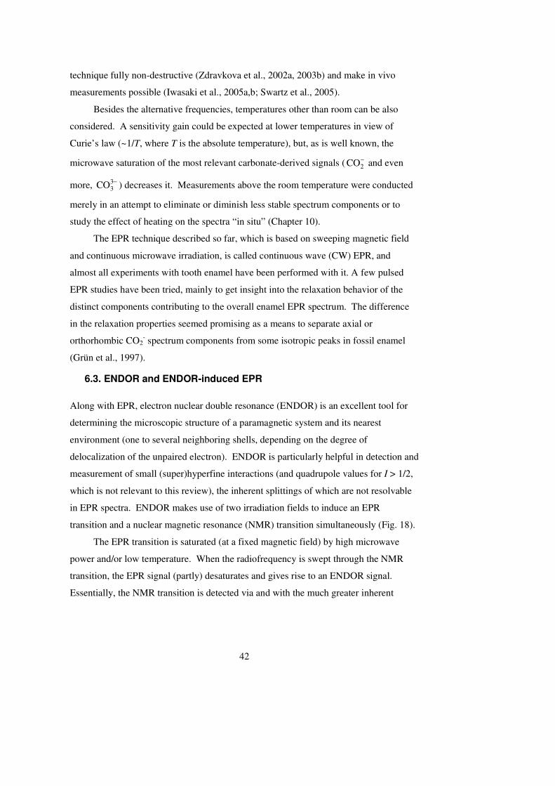
42

technique fully non-destructive (Zdravkova et al., 2002a, 2003b) and make in vivo

measurements possible (Iwasaki et al., 2005a,b; Swartz et al., 2005).

Besides the alternative frequencies, temperatures other than room can be also

considered. A sensitivity gain could be expected at lower temperatures in view of

Curie’s law (~1/T, where T is the absolute temperature), but, as is well known, the

microwave saturation of the most relevant carbonate-derived signals ( 2CO− and even

more, 33CO − ) decreases it. Measurements above the room temperature were conducted

merely in an attempt to eliminate or diminish less stable spectrum components or to

study the effect of heating on the spectra “in situ” (Chapter 10).

The EPR technique described so far, which is based on sweeping magnetic field

and continuous microwave irradiation, is called continuous wave (CW) EPR, and

almost all experiments with tooth enamel have been performed with it. A few pulsed

EPR studies have been tried, mainly to get insight into the relaxation behavior of the

distinct components contributing to the overall enamel EPR spectrum. The difference

in the relaxation properties seemed promising as a means to separate axial or

orthorhombic CO2- spectrum components from some isotropic peaks in fossil enamel

(Grün et al., 1997).

6.3. ENDOR and ENDOR-induced EPR

Along with EPR, electron nuclear double resonance (ENDOR) is an excellent tool for

determining the microscopic structure of a paramagnetic system and its nearest

environment (one to several neighboring shells, depending on the degree of

delocalization of the unpaired electron). ENDOR is particularly helpful in detection and

measurement of small (super)hyperfine interactions (and quadrupole values for I > 1/2,

which is not relevant to this review), the inherent splittings of which are not resolvable

in EPR spectra. ENDOR makes use of two irradiation fields to induce an EPR

transition and a nuclear magnetic resonance (NMR) transition simultaneously (Fig. 18).

The EPR transition is saturated (at a fixed magnetic field) by high microwave

power and/or low temperature. When the radiofrequency is swept through the NMR

transition, the EPR signal (partly) desaturates and gives rise to an ENDOR signal.

Essentially, the NMR transition is detected via and with the much greater inherent

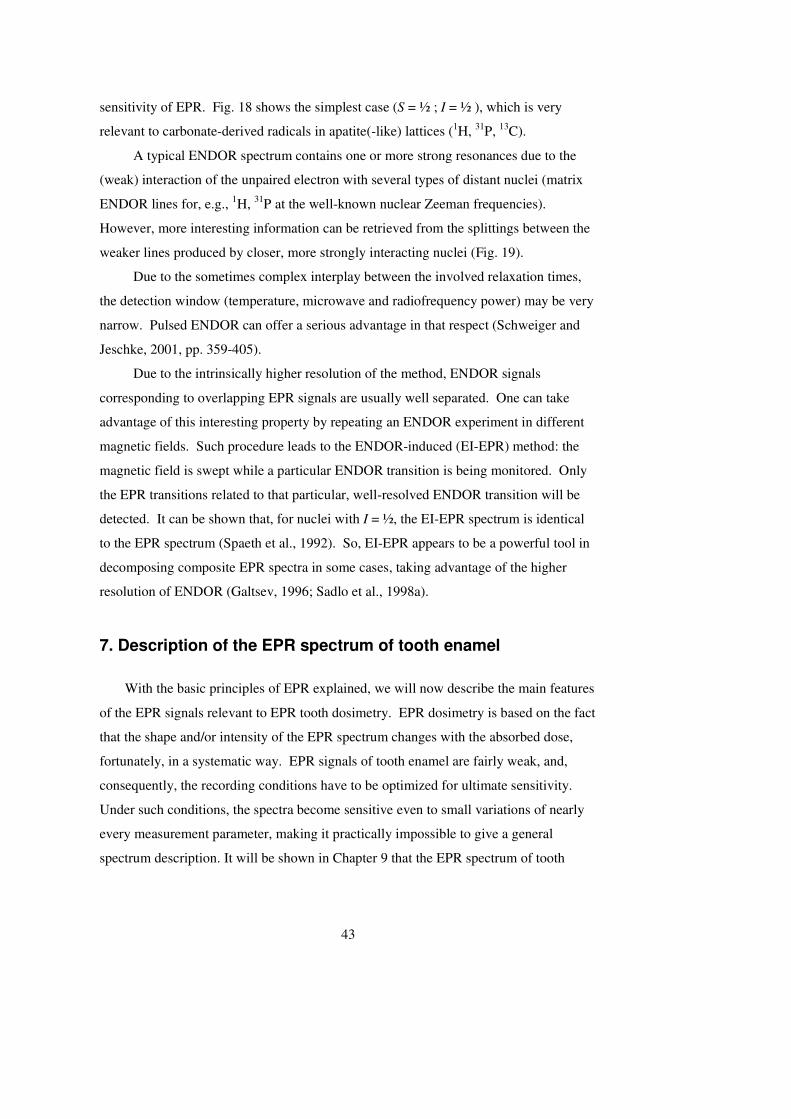
43

sensitivity of EPR. Fig. 18 shows the simplest case (S = ½ ; I = ½ ), which is very

relevant to carbonate-derived radicals in apatite(-like) lattices (1H, 31P, 13C).

A typical ENDOR spectrum contains one or more strong resonances due to the

(weak) interaction of the unpaired electron with several types of distant nuclei (matrix

ENDOR lines for, e.g., 1H, 31P at the well-known nuclear Zeeman frequencies).

However, more interesting information can be retrieved from the splittings between the

weaker lines produced by closer, more strongly interacting nuclei (Fig. 19).

Due to the sometimes complex interplay between the involved relaxation times,

the detection window (temperature, microwave and radiofrequency power) may be very

narrow. Pulsed ENDOR can offer a serious advantage in that respect (Schweiger and

Jeschke, 2001, pp. 359-405).

Due to the intrinsically higher resolution of the method, ENDOR signals

corresponding to overlapping EPR signals are usually well separated. One can take

advantage of this interesting property by repeating an ENDOR experiment in different

magnetic fields. Such procedure leads to the ENDOR-induced (EI-EPR) method: the

magnetic field is swept while a particular ENDOR transition is being monitored. Only

the EPR transitions related to that particular, well-resolved ENDOR transition will be

detected. It can be shown that, for nuclei with I = ½, the EI-EPR spectrum is identical

to the EPR spectrum (Spaeth et al., 1992). So, EI-EPR appears to be a powerful tool in

decomposing composite EPR spectra in some cases, taking advantage of the higher

resolution of ENDOR (Galtsev, 1996; Sadlo et al., 1998a).

7. Description of the EPR spectrum of tooth enamel

With the basic principles of EPR explained, we will now describe the main features

of the EPR signals relevant to EPR tooth dosimetry. EPR dosimetry is based on the fact

that the shape and/or intensity of the EPR spectrum changes with the absorbed dose,

fortunately, in a systematic way. EPR signals of tooth enamel are fairly weak, and,

consequently, the recording conditions have to be optimized for ultimate sensitivity.

Under such conditions, the spectra become sensitive even to small variations of nearly

every measurement parameter, making it practically impossible to give a general

spectrum description. It will be shown in Chapter 9 that the EPR spectrum of tooth

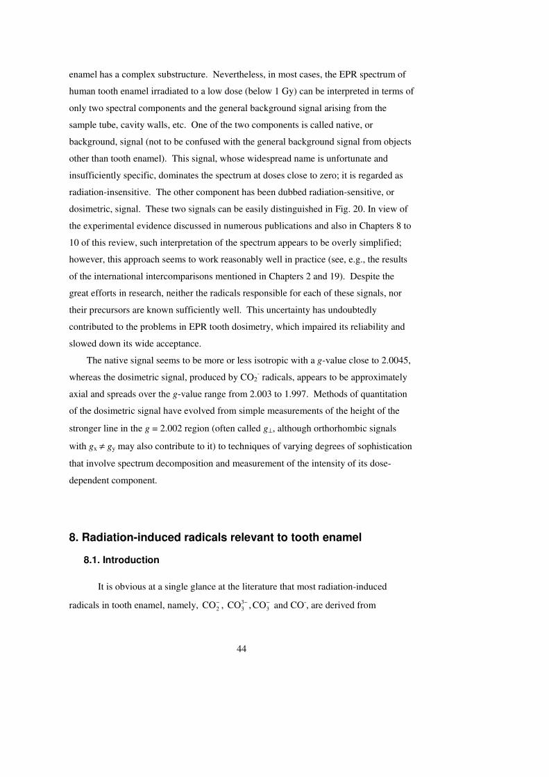
44

enamel has a complex substructure. Nevertheless, in most cases, the EPR spectrum of

human tooth enamel irradiated to a low dose (below 1 Gy) can be interpreted in terms of

only two spectral components and the general background signal arising from the

sample tube, cavity walls, etc. One of the two components is called native, or

background, signal (not to be confused with the general background signal from objects

other than tooth enamel). This signal, whose widespread name is unfortunate and

insufficiently specific, dominates the spectrum at doses close to zero; it is regarded as

radiation-insensitive. The other component has been dubbed radiation-sensitive, or

dosimetric, signal. These two signals can be easily distinguished in Fig. 20. In view of

the experimental evidence discussed in numerous publications and also in Chapters 8 to

10 of this review, such interpretation of the spectrum appears to be overly simplified;

however, this approach seems to work reasonably well in practice (see, e.g., the results

of the international intercomparisons mentioned in Chapters 2 and 19). Despite the

great efforts in research, neither the radicals responsible for each of these signals, nor

their precursors are known sufficiently well. This uncertainty has undoubtedly

contributed to the problems in EPR tooth dosimetry, which impaired its reliability and

slowed down its wide acceptance.

The native signal seems to be more or less isotropic with a g-value close to 2.0045,

whereas the dosimetric signal, produced by CO2- radicals, appears to be approximately

axial and spreads over the g-value range from 2.003 to 1.997. Methods of quantitation

of the dosimetric signal have evolved from simple measurements of the height of the

stronger line in the g = 2.002 region (often called g⊥, although orthorhombic signals

with gx ≠ gy may also contribute to it) to techniques of varying degrees of sophistication

that involve spectrum decomposition and measurement of the intensity of its dose-

dependent component.

8. Radiation-induced radicals relevant to tooth enamel

8.1. Introduction

It is obvious at a single glance at the literature that most radiation-induced

radicals in tooth enamel, namely, 2CO− , 33CO − , 3CO− and CO-, are derived from

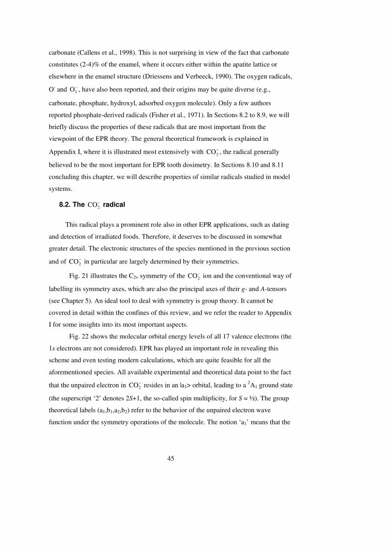
45

carbonate (Callens et al., 1998). This is not surprising in view of the fact that carbonate

constitutes (2-4)% of the enamel, where it occurs either within the apatite lattice or

elsewhere in the enamel structure (Driessens and Verbeeck, 1990). The oxygen radicals,

O- and 3O− , have also been reported, and their origins may be quite diverse (e.g.,

carbonate, phosphate, hydroxyl, adsorbed oxygen molecule). Only a few authors

reported phosphate-derived radicals (Fisher et al., 1971). In Sections 8.2 to 8.9, we will

briefly discuss the properties of these radicals that are most important from the

viewpoint of the EPR theory. The general theoretical framework is explained in

Appendix I, where it is illustrated most extensively with 2CO− , the radical generally

believed to be the most important for EPR tooth dosimetry. In Sections 8.10 and 8.11

concluding this chapter, we will describe properties of similar radicals studied in model

systems.

8.2. The 2CO− radical

This radical plays a prominent role also in other EPR applications, such as dating

and detection of irradiated foods. Therefore, it deserves to be discussed in somewhat

greater detail. The electronic structures of the species mentioned in the previous section

and of 2CO− in particular are largely determined by their symmetries.

Fig. 21 illustrates the C2v symmetry of the 2CO− ion and the conventional way of

labelling its symmetry axes, which are also the principal axes of their g- and A-tensors

(see Chapter 5). An ideal tool to deal with symmetry is group theory. It cannot be

covered in detail within the confines of this review, and we refer the reader to Appendix

I for some insights into its most important aspects.

Fig. 22 shows the molecular orbital energy levels of all 17 valence electrons (the

1s electrons are not considered). EPR has played an important role in revealing this

scheme and even testing modern calculations, which are quite feasible for all the

aforementioned species. All available experimental and theoretical data point to the fact

that the unpaired electron in 2CO− resides in an |a1> orbital, leading to a 2A1 ground state

(the superscript ‘2’ denotes 2S+1, the so-called spin multiplicity, for S = ½). The group

theoretical labels (a1,b1,a2,b2) refer to the behavior of the unpaired electron wave

function under the symmetry operations of the molecule. The notion ‘a1’ means that the

46

wave function is not affected by any symmetry operation (e.g., the spherically

symmetrical carbon 2s-orbital makes a part of it, but also the 2pz orbital with axial

symmetry with respect to the z-axis). Placing such a molecule in a crystal lattice or in

some other environment will not induce any additional level splitting (only a magnetic

field as applied in EPR can lift the remaining twofold degeneracy between the spin-up

and spin-down states) and will, in general, have only a minor effect on the electronic

structure. This was confirmed experimentally and computationally (Atkins and Symons,

1967). This explains why g- and A-values of 2CO− (also of -

3O with the same symmetry)

are nearly the same for many systems and why we can understand the essential features

of this molecular ion by studying it in its simplest form, i.e., the free state depicted in

Fig. 21.

The presence of the carbon 2s-function in the ground state wave function (see

Appendix I, Eq. (I.1)) is the reason for a large isotropic 13C hyperfine coupling of about

15 mT. As mentioned above, the 2pz-component will make the hyperfine tensor (nearly)

axial with Az being the largest value. The 17O hyperfine tensor can also be analyzed

using the last three terms in Eq. (I.1) of Appendix I in order to confirm the radical

identification, but we will not discuss this here (for a good example, see an analysis of

the spectrum of 2CO− in MgO by Meriaudeau et al., 1975).

It immediately follows from the C2v symmetry of the molecular ion that the g-

tensor must be orthorhombic in the real sense (Chapter 5) and not axial (unless the

molecule is rotating). Essentially from the symmetry and by inspecting Fig. 22, one can

show that

∆gy = gy – ge < 0, |∆gy | >> |∆gx |, |∆gz |, gx > gz > gy . (8.1)

The most important feature of the static 2CO− molecular ion is its smallest g-

value (gy) along the O-O axis, which is about 1.997 (±0.001) in all cases. This

represents a relatively large deviation from ge for such types of molecules. Typical

values for the other principal directions are gx = 2.0030 and gz = 2.0015. The average of

the three principal values is usually approximately 2.0006 (Section 8.10). In the early

literature, 2CO− was confused with 33CO − (see next section) because both of these

carbonate-derived molecular ions have the same type of ground state (A1).

8.3. The 33CO − radical

47

This molecular ion has 25 valence electrons and a pyramidal structure (C3v

symmetry). The main symmetry axis is threefold; it is usually labelled as z. Although

the unpaired electron in this species is also in an |a1> orbital, there is an important

difference from the 2CO−

radical. When the symmetry group is C3v, the x and y

directions in the plane containing the three oxygen atoms, perpendicular to the

symmetry axis, are completely equivalent. This gives rise to energy levels with a

degeneracy higher than two, at variance with the 2CO− radical. This means that four

electrons can be accommodated at certain levels and that such levels will be split into

two doublets by a perturbation that lowers the symmetry (e.g., a neighbouring defect).

Thus, the environment of the radical will have a relatively strong effect on the spin

Hamiltonian parameters. A consequence of the aforementioned equivalency for a free

ion is gx = gy and that the radical has axial g and A tensors. Perturbations making x and y

directions non-equivalent will render gx ≠ gy.

All available experimental and theoretical data point to small deviations of the

symmetry from axiality and small deviations of all g-values from ge (Callens et al.,

1991; Sadlo et al., 1998b; Vanhaelewyn et al., 2002a). Typically, gx ≅ gy ≅ 2.0030 –

2.0045 and gz ≅ 2.0010 – 2.0020. The average g-value is very close to that of a free

electron.

In view of the carbon part of the ground state wave function (s and pz, see Appendix I),

|a1> = c1s + c2pz + … oxygen part, (8.2)

the 13C A-tensor is qualitatively and even quantitatively comparable to the one of 2CO− ,

but the largest A-value is now found along the direction with the smallest g-value, in

contrast to the 2CO− radical. Using also the gy-feature of 2CO− , it is thus possible, albeit

not always easy, to differentiate between these two radicals.

8.4. The 3CO− radical

While 33CO − is presumably produced from the non-paramagnetic 2

3CO − ions by

electron trapping, hole capture generates 3CO− ions (the electrons and holes are formed,

e.g., under irradiation). The ion is planar (D3h symmetry) and has 23 valence electrons.

The threefold symmetry axis (z-axis) is perpendicular to the molecular plane. By

analogy with 33CO − , certain energy levels of the free 3CO− ion are fourfold degenerate

48

(twofold orbital and twofold spin degeneracy) and are, thus, sensitive to perturbations

breaking the threefold symmetry. This radical has a ground state of a different

symmetry type than 2CO− and 33CO − , which is not invariant under the symmetry

operations of the D3h group. It is essentially built from oxygen atomic orbitals and,

because the carbon part is absent, the 13C hyperfine couplings are theoretically equal to

zero (in practice, they are very small). When 13C data are available, 3CO− can be easily

distinguished from 2CO− and 33CO − . The g-tensor is axial for the free ion for the same

reasons as for 33CO − . All the g-values seem to be larger than ge. For gx (= gy), values

above 2.015 were frequently reported. Thus, 3CO− can hardly be confused with 2CO− or

33CO − . However, in samples that are not 13C-enriched, its signal may be mixed up with

signals of certain oxygen radicals (see below).

8.5. The CO- radical

This is probably the least known carbonate-derived radical, and its identification

is not simple. Similar problems were encountered in the investigations of the

isoelectronic NO-molecule, which caused a lot of controversy in the EPR literature

(Atkins and Symons, 1967). This ion has 11 valence electrons and C∞v symmetry

implying many orbitally degenerate levels. The ground state is most probably 2Π. The

twofold orbital degeneration is expected to lead to a considerable dependence of the

EPR signal on the environment. To the best of our knowledge, no other EPR properties

of this radical have been described in the literature, likely due to the small amount of

available experimental data and the theoretical speculations mentioned above.

8.6. The O3- radical

This radical has been reported in a small number of enamel-related papers, mainly

in those describing studies of synthetic apatite. However, it is advisable to be aware of

its possible presence in tooth enamel. Its theoretical treatment is similar to the treatment

of 2CO− , which has the same C2v-symmetry. The carbon atom is replaced by the central

oxygen, which is not equivalent to the two outer equivalent oxygen atoms. Thus, 3O−

has 19 valence electrons, and the unpaired electron occupies the next highest |b1> level

49

(Fig. 22). The axis labelling is the same as for 2CO− , and the paramagnetic electron

resides in px-type orbitals perpendicular to the molecular plane. Again, the main features

of the g-tensor for the free ion can be derived from symmetry and Fig. 22:

gy > gz > gx ≅ ge.

This radical is clearly orthorhombic, and its typical g-values, which will be only weakly

affected by the crystal environment, are gx = 2.003, gy = 2.018, and gz = 2.012.

8.7. The O- radical

The free O- ion has five 2p electrons (2p5 configuration), and only one electron is

lacking to fill the 2p shell completely. It is well known that such a “hole configuration”

can be treated theoretically in the same way as the configuration of a system with a

single p-electron (Abragam and Bleaney, 1970, p. 744). The ground state is 2P; it has a

threefold orbital (there are 3p-functions, px, py and pz) and a twofold spin degeneracy.

As a consequence of the threefold orbital degeneracy, the environment will have a

considerable effect on its electronic structure, and thus, its g and A tensors. Axial and

orthorhombic varieties, as well as conformations with even lower symmetry, are a priori

possible. (Cubic symmetry with isotropic g and A tensor is ruled out because of the

Jahn-Teller effect (Abragam and Bleaney, 1970, Chapter 21)). This implies that “typical

g-values” for O- do not really exist and identification based solely on the g-tensor is

never very convincing. Ideally, enrichment with 17O is required, but this is not realistic

for tooth enamel. Other arguments (considerations of precursors, doping, etc.) may be

valuable, but they are fairly indirect.

It can be shown that one g-value (gz), which corresponds to the direction of the

lobe containing the unpaired electron, is close to and slightly smaller than ge, whereas

the other two principal values can be as high as 2.3. Values of about 2.06 – 2.08 have

been reported for gx and gy in apatites (Section 8.11).

8.8. The superoxide radical O2-

The superoxide ion has 13 valence electrons, a D∞h symmetry and a 2Πg ground

state (twofold orbital and twofold spin degeneracy). The axiality is reflected in the axial

g-tensor with g// = 4 and g⊥ = 0 (Zeller and Känzig, 1967). Incorporating the radical into

a lattice environment will lower its symmetry and affect the principal values

50

considerably, but it has been found that the g-tensor remains nearly axial with g// > ge

and g⊥ ≅ ge. Theoretical formulas for the g-values have been derived, e.g., by Zeller and

Känzig (1967). (See also Section 8.11 for experimental examples).

8.9. Phosphate radicals

PO42- is the only phosphate radical that may be of some relevance to tooth

dosimetry. This radical has 31 valence electrons and a slightly distorted tetrahedral

structure. According to Atkins and Symons (1967), this should result in at least one g-

value considerably larger than ge and small 31P hyperfine couplings. It seems unlikely to

observe this radical at room temperature in view of its expected strong interaction with

the surrounding lattice. Further theoretical information on this radical is hardly

available in the literature. Some experimental data will be given in Section 8.11.

8.10. Carbon-containing radicals in tooth enamel model systems

Having described the basic features of the radicals potentially relevant to an

analysis of tooth enamel spectra, we will now present some illustrative literature data. It

was not our intention to provide an exhaustive literature review, and the following is

restricted, as much as possible, to reliable “model systems”, such as single crystals

and/or isotopically enriched samples. Table 5 summarizes the principal g-values of CO2-

, CO33-, CO3

- and CO- in a variety of lattices. The 13C-hyperfine couplings for these

carbon-containing ions are also given in most cases.

CO2-

A pioneering study of CO2- was carried out on sodium formate samples (Ovenall

and Whiffen, 1961). The interpretation of the spectra, based largely on a comparison

with NO2 (Atkins et al., 1962), can be considered nowadays as doubtless. Table 5 shows

that the spin Hamiltonian parameters for CO2- are extremely insensitive to the

environment. This is also the case for the other ions, but to a lesser extent, in agreement

with the theoretical predictions in the sections above. This means that a discrimination

between these radicals should not pose any problems, even if only the principal g-values

are available. However, there may be problems with oxygen and carbonate radicals

containing or interacting with a hydrogen nucleus (see below).

51

The most relevant model system for tooth enamel is a carbonate-containing

hydroxyapatite single crystal. However, we are aware of only one study on radiation-

induced carbonate-derived radicals (Vanhaelewyn et al., 2000b). Probably because of

the small sample size and the low carbonate content, only two, slightly different, CO2-

radicals could be identified. Both the radicals were found to have g-tensors axial with

respect to the hexagonal c-axis. It can be expected that these bulk radicals are

omnipresent in apatite-containing samples. Of course, they can be obscured by

contributions from other, e.g., surface-related radicals in systems with larger surface-to-

volume ratios.

In our opinion, the best model systems to identify carbonate radicals and to

study their behavior are calcite single crystals. They have trigonal symmetry

(compatible with hexagonal apatite), and their EPR spectra consist of extremely narrow

lines, mainly due to the low abundance of lattice nuclei with nonzero nuclear spins.

Moreover, with the exception of CO-, all carbonate-derived radicals relevant to tooth

dosimetry have been detected in this material, some even in different varieties.

To recapitulate, the CO2- radical is basically orthorhombic, but, at room

temperature, axial varieties certainly exist as well. Some of these represent CO2- ions

rotating about the axis perpendicular to the molecular plane (McMillan and Marshall,

1968). This results in g// = gx and the other two g-values averaged to g⊥ (destroying the

g = 1.997 feature in this case!). In other cases, the CO2- ion is rotating about the O-O

axis corresponding to gy (Vanhaelewyn et al., 2000b; Callens et al., 1989a), and the gx

and gz values are averaged. In some samples, even centers with completely isotropic g-

tensors have been found; most probably, that was due to rapid tumbling of the radicals

in the presence of water, perhaps occluded (Callens et al., 1989b; Moens et al., 1995).

In addition to bulk radicals, surface CO2- radicals have been described. In our

opinion, the most convincing and complete study was presented by Meriaudeau et al.

(1975). Making use of 13C- and 17O-enriched CO and CO2 gases, the authors identified a

symmetric CO2- ion and a slightly asymmetric O-CO- molecular ion on a MgO surface

by reaction of surface O- ions with CO (Table 5). The results of the analysis of the 13C

and 17O hyperfine tensors were completely consistent with the theory. The 17O

hyperfine values measured in this work are in good agreement with the values reported

52

later for CO2- radicals in NaHCO2 single crystals by Schlick et al. (1971). According to

these studies, the O-C-O bond angles vary between 130° and 140°.

A general property of all reported CO2- radicals is their very high stability. We

are not aware of any studies reporting a noticeable decay within a year. In some

samples, these radicals are stable for hundreds of thousands of years; this extraordinary

stability has become a foundation of EPR dating (Ikeya, 1993).

CO33-

The other carbon-containing radical ions show significantly lower thermal

stabilities. For example, the signal of axial CO33- in calcite decreases to about one fourth

of its initial intensity within one day. However, this ion may be stabilized by a

neighbouring defect (e.g., a cation impurity or a vacancy). Centers stabilized by Y3+,

Sc3+ and Li+ have been reported (Marshall and McMillan, 1968; Bacquet et al., 1975;

Mineyeva et al., 1993). When the stabilizing cation is not on the symmetry axis of the

free ion, the CO33- center may become orthorhombic (Table 5). In addition to the g =

1.997 feature of the CO2-, CO3

3- can be distinguished from CO2- by the fact that its

largest hyperfine coupling is for the same direction as its smallest g-value. The CO2-

splittings are somewhat larger, but this is a less discriminating feature. As outlined in

the following chapters, heat treatment before irradiation can strongly increase the

stability of CO33-.

Another distinguishing feature of the CO33- ion is the easy power saturation of its

signal. The saturation is observable even at relatively low microwave powers (0.1 – 1

mW), whereas saturation of the signals of CO2- and CO3

- may get noticeable only at 5-

10 mW and sometimes (for isotropic centers) does not occur even at the maximal

available microwave power of 200 mW.

CO3-

The least stable carbonate-derived ion of all is CO3- (in calcite, its decay times

are in the range of tens of minutes even at low temperatures). Like the CO33- ion, it can

become stable after heating (see below). In practice, this signal will only weakly, if at

all, interfere with the signals used for dosimetry: apart from its low thermal stability, its

g-values are too high to cause a serious overlap. This may be different for the native

53

signal around g = 2.0045. When 13C data are available, the couplings observed for this

ion are roughly one order of magnitude smaller than for the two carbonate-derived

radicals mentioned above. Orthorhombic, axial and isotropic (rapidly tumbling)

varieties have been reported (Table 5 and Callens et al., 1989b).

CO-

Finally, we will give some attention to the most mysterious, but perhaps quite

important for tooth dosimetry radical, namely, CO-. Its occurrence has been reported

only a few times, and its theory seems to be understood to a lesser degree. Assignments

go back essentially to the work by Lunsford and Jaine (1966). Table 5 shows that the g-

values are spread around 2.0045 (in fact, exactly in the position of the native signal of

tooth enamel). Moreover, it has been found on the surface of unirradiated MgO

(Lunsford and Jaine, 1966). In two other studies, samples had been irradiated, but it

cannot be ruled out entirely that the unirradiated samples had the same signal (Moens et

al., 1991; Schramm and Rossi, 1999).

Carbonate-derived radicals containing and/or interacting with

hydrogen

Another category of less studied and, hence, less known radicals are those with

an involved hydrogen atom. Adding a proton to the radicals discussed above may result

in other paramagnetic entities, which should be, in principle, recognizable by their extra

hydrogen hyperfine coupling.

Chantry and Whiffen (1962) reported a species, which they described as

CO2(H), in KHCO3 single crystals. The hydrogen couplings were below 15 MHz for all

orientations and, therefore, could not be resolved. The g-tensor and 13C-hyperfine values

would certainly lead to identification of CO2- (Table 6), and this possibility was not

ruled out by the authors (the proton interaction then being due to a hydrogen bridge). A

correct line assignment (and spectrum fitting) for such a radical in tooth enamel would

not be easy, if at all possible. The enamel structure contains enough protons for a

possible association or bond with CO2-.

The HCO32- radical was identified in a CaCO3 single crystal by Cass et al.

(1974). It has a well-resolved hydrogen splitting of about 3.6 mT and may be confused

54

only with a phosphate radical (31P has also I = ½). Overlapping the central signals is not

likely.

No problems are expected from the HCO- radical, which has been identified in

irradiated hydroxyapatite powders by Schramm and Rossi (1999). It is mentioned here

just for completeness. Its average 1H hyperfine splitting is approximately 9 mT.

In conclusion, it seems that only CO2(H) radicals have to be taken into account

seriously within this class of radicals.

8.11. Oxygen and phosphate radicals in tooth enamel model systems

We start our discussion with the simplest oxygen radical, i.e., O-. The most

relevant work was carried out on HAp single crystals by Mengeot et al. (1974). This

work was very unique because sufficiently large hydroxyapatite single crystals of good

quality were scarce (Mengeot et al., 1973, 1974). Although this radical is unobservable

in such crystals at room temperature (after irradiation either at room temperature or at

77 K), its g-tensor of g// = 2.0018 and g⊥ = 2.0683 (axial with respect to the pseudo-

hexagonal c-axis) indicates potential significance of this species for EPR dosimetry.

The precursor is OH- ion, which produces O- when radiation removes the

hydrogen atom. Furthermore, superhyperfine interaction with a proton of a neighboring

hydroxyl group has been reported (Mengeot et al., 1973, 1974). As mentioned in the

theoretical part, a reliable identification of such centers in non-model systems is not

easy because of the absence of hyperfine structure and possible confusion with other

oxygen radicals. Therefore, in order to give an idea of typical g-values that can be

expected in tooth enamel a priori, we quote the g-values of two similar bulk centres in

chlorapatite reported by the same group (Roufosse et al., 1974): g// = 2.0031 and g⊥ =

2.0255; g// = 2.0032 and g⊥ = 2.0386 (both axial with respect to the c-axis). Again, the

precursors are hydroxyl ions. In the study by Meriaudeau et al. (1975), a surface O- ion

was identified with the following g-tensor: gx = 2.041; gy = 2.039; gz = 2.0010.

It is clear that, in powder samples, the differentiation between bulk and surface

radicals is not easy. Furthermore, orthorhombic g-tensors can be expected in the bulk

(for instance, varieties with a small perturbation). This implies that orthorhombicity

55

cannot be used as a criterion to decide whether or not a radical is located in the bulk or

at the surface.

The importance of these centres for tooth dosimetry stems from the presence of a

sometimes intense (due to its relatively narrow line) purely negative gz signal (“leg”) in

the region near g = 2, where it may complicate the spectrum analysis (see, e.g., Fig. 3 of

Meriaudeau et al. 1975).

Only very few papers reported superoxide (O2-) ions in apatite-related materials.

One cannot rule out entirely that their spectra may have been mixed up with those of,

e.g., O- ions or that their presence may have been overlooked. Rey et al. (1976)

identified O2- radicals in oxygenized apatite powders (g// = 2.05; g⊥ = 2.00). These g

values are comparable to those found in calcite by Meguro and Ikeya (1993): g// =

2.069; g⊥ = 2.009. The g-values of the superoxide ions may depend on the lattice

substantially, but will remain nearly axial, as was demonstrated with KCl single crystals

(see below). The typical g-values for an ozonide (O3-) radical, which may occur in tooth

enamel under certain circumstances, in KCl are:

O2- : gx = 1.9512; gy = 1.9551; gz = 2.4360 (Zeller and Känzig, 1967);

O3- : gx = 2.0032; gy = 2.0182; gz = 2.0118 (Callens et al., 1988).

The g-values for the ozonide ion are very insensitive to the environment of the ion,

either in the bulk or at the surface. Ozonide has also been identified in synthetic apatites

with similar g-values (Van Doorslaer et al., 1996). Low-temperature ashing appeared to

be necessary for detecting this ion in tooth enamel and bone (Tochon-Danguy et al.,

1978).

We conclude this chapter with a few literature results for PO42-. The spectra are

very unstable at room temperature, and low temperatures are necessary for both sample

irradiation and spectrum registration, as predicted from the theoretical considerations.

Fisher et al. (1971) reported the following spin Hamiltonian parameters for this ion in

calcium phosphate:

g// = 2.030; g⊥ = 2.0062; A// = 2.20 mT; A⊥ = 3.08 mT.

In spectra of synthetic apatite powders, Peckauskas and Pullman, 1978b observed only

the perpendicular 31P doublet. More recently, the typical perpendicular splitting was

observed in preheated tooth enamel, which had been irradiated and measured at low

temperatures (Sadlo et al., 1998b). This radical is probably relevant only to fundamental

Met opmaak: Frans(standaard)

56

studies, but it is worth noting that its highest-field feature in the X band coincides nearly

perfectly with gy (1.997) of the CO2- signal.

9. EPR signals induced by ionizing radiation in tooth enamel

9.1. Introduction

In this chapter, we will try to sketch out the latest insights into the radicals

responsible for the enamel spectrum, already briefly discussed earlier (Chapter 7). We

will restrict ourselves to the spectrum recorded at room temperature after irradiation at

room temperature. The native signal present without irradiation will be treated in the

next chapter, and the discussion here is thus confined to what is commonly called

dosimetric signal. It is also not our aim to give an exhaustive review of all papers ever

published in this field. We will essentially discuss the papers that, in our humble

opinion, contributed substantially to our present understanding of the dosimetric signal

in human tooth enamel. For obvious reasons, most fundamental studies have been

performed on samples irradiated to high doses (in the kGy range).

9.2. Type of radicals

It became clear at an early stage that carbon-containing radicals significantly

contributed to what was called “asymmetric signal near g = 2” (AS) (see, e.g., Chapter

5, Fig. 17). The carbon involvement was clearly demonstrated when Cevc et al. (1972)

found rather broad 13C hyperfine signals approximately 17 mT apart, centered around

AS, and about 100 times smaller in intensity than the latter.4 At that time, the signal

was thought to be non-composite and was erroneously attributed to CO33-. The reported

g-values, g⊥ = 2.0036 and g// = 1.9983, were overestimated by approximately 0.0013,

probably due to an inaccurate field and/or frequency calibration. (It is worth noting that

comparison of newer data with those in the older literature is often hampered by very

poor earlier description of the experimental conditions, like microwave power and

modulation amplitude values, small and unclear figures, and other similar factors.)

4 It is important to clearly distinguish between the amplitude (peak-to-peak height) and the intensity of an EPR signal, the latter being proportional to the amplitude times the maximum-to-minimum line width squared.

57

Doi et al. (1979) and Sato (1979) found the same or very similar satellite lines with

an amplitude of about 1000 times smaller than the central signal (in view of the larger

line width, this could correspond to the 1% intensity mentioned above). From Q-band

measurements (Doi et al. 1980), three distinct g-values were reported, gx = 2.0028, gy =

1.9971, and gz = 2.0018 (the latter signal/shoulder at 2.0018 was, in fact, attributed to

another species). Next to the broad doublet of 17 mT, Doi et al. (1981a) also found

traces of an isotropic doublet with a splitting of 14.6 mT. In a more recent study by

Ishchenko et al. (2002), the 13C line shapes with the 17-mT splitting were fitted by a

superposition of an orthorhombic and an axial CO2- signal:

- axial: g⊥ = 2.0023 ; g// = 1.9975 ; A⊥ = 550 MHz ; A// = 460 MHz (radical rapidly

rotating about the O-O axis parallel with the hexagonal c-axis);

- orthorhombic: gx = 2.0030 ; gy = 1.9975 ; gz = 2.0015

Ax = 480 MHz ; Ay = 460 MHz ; Az = 550 MHz.

The axial signal was found to increase relatively when the samples were annealed above

150 °C. The individual 13C signals could only be resolved by a computer fitting, and

the apparent splitting increased roughly by 1 mT with annealing temperature (induced

by the growth of the axial signal).

There is a wide consensus nowadays that the involved carbon-containing centers

are CO2- radicals and that their earlier assignments to CO3

3- were erroneous. Bacquet et

al. (1981), Geoffroy et al. (1985) and Callens et al. (1987) all advocated CO2- as the

(dominant) radical in both enamel and most synthetic apatites. In addition to the critical

features described in the theoretical Chapter 8 (the 1.997 feature, the largest 13C

coupling corresponding to gz, and the intermediate g-value), the following two very

convincing arguments support this claim. It is clear from Fig. 13 of Chapter 5 that

simulated typical CO2- and CO3

3- powder spectra are quite different and that only the

CO2- signal corresponds to the experimental AS or dosimetric signal at sufficiently high

doses (above 1 Gy). Furthermore, the “true” CO33- signals have been identified in both

synthetic apatites and (heated) tooth enamel (Callens et al., 1991; Sadlo et al., 1998b;

and Vanhaelewyn et al., 2002a). Fig. 5 in a paper by Sadlo et al. (1998b) is particularly

illustrative in terms of the relative positions of the typical CO2- and CO3

3- powder

components.

58

It has become clear in the recent years that the CO2- spectrum has a finer

substructure, although most enamel powder spectra can be approximated reasonably

well by a simple CO2- theoretical spectrum (depending, however, on, e.g., the

microwave power; see Fig. 17 of Chapter 5). By using enamel blocks (plates) preheated

at 400 °C before irradiation, Callens et al. (1995b) showed that (at least) two types of

CO2- ions coexist in unheated enamel. The first type is probably a bulk CO2

-, which

shows an anisotropic signal in the partially ordered blocks (often referred to as

“oriented” radicals). The second type shows no anisotropy (not even in blocks) and,

thus, exhibits an (orthorhombic) powder spectrum. The latter signal can be eliminated

or at least drastically reduced by preheating for 2-3 weeks at 400 °C. It is probably due

to a surface radical or a radical “loosely” attached between the apatite crystallites in the

enamel structure (“disordered” radicals).

Fig. 23 indeed demonstrates that the spectra of preheated and untreated blocks are

clearly different, in contrast to what was found for the corresponding powder spectra.

Fig. 23 shows that the difference between the “preheated” and “untreated” spectra can

be attributed to a powder spectrum from “disordered” CO2- radicals (Callens et al.

1995b).

A Q-band study by Vanhaelewyn et al. (2002b) added considerable support for

these conclusions. The g-tensors of both radicals are so similar that the signals cannot

be separated even in Q-band, although some evidence could be found that the

orientation-dependent component shows a larger anisotropy than the orientation-

independent one. This is fully compatible with the fact that the CO2- g-values are very

insensitive to environmental changes. The fact that the 13C-features are more sensitive

to annealing than the central part, which is determined solely by the g-tensor, can also

be interpreted in the same way (Ishchenko et al., 2002). Existence of a finer

substructure in the CO2- spectrum was also confirmed by the works by Ishchenko et al.

(1999) and Brik et al. (1998, 2000c). The latter work will be discussed in detail below.

9.3. Symmetry of the radicals (isotropic, axial, orthorhombic)

Because of the wider lines, it is not easy to determine whether the involved CO2-

components are axial or orthorhombic, certainly not in the X-band where the (possible)

gz component around 2.0015 is not resolved at all. It is quite obvious from the studies

59

by Vanhaelewyn et al. (2002a,b) that Q- and W-band spectra of unheated enamel

comprise a strong orthorhombic CO2- component (resolved features at gz = 2.0016 next

to gy = 1.9970 and gx in the vicinity of 2.0030) along with a small isotropic CO2-

contribution at g = 2.0007 (CO2- in occluded water, Callens et al. 1995a, Moens et al.,

1995). The latter is most likely the same signal as detected by Doi et al. (1981a),

exhibiting the splitting of 14.6 mT (see above). Although numerous publications (e.g.,

Murata et al., 1993; Murata et al., 1996) point to the relation of this isotropic signal with

the presence of water, Vorona et al. (2005) has surprisingly found that the same (?)

signal in enamel increases on heating to 230 °C. Vanhaelewyn et al. (2002b) found the

opposite from well-resolved Q-band spectra.

Preheating decreases the relative intensity of the gz-feature around 2.0016, which

may point to a growing importance of the axial CO2- component (same gy = 1.9970, and

gx still around 2.0030). This is in agreement with the 13C study by Ishchenko et al.

(2002), which revealed that the axial component was growing in the process of the

preheating. That observation was interpreted as a result of a conversion of disordered

radicals into oriented ones. A recent publication by the same group (Vorona et al.,

2006) reports that an annealing of irradiated samples (for 20 minutes at temperatures up

to 320 °C) resulted in a transformation of orthorhombic CO2- centers into axial ones. It

was concluded that both the CO2- types should be present at B-sites. Q-band results by

Vanhaelewyn et al. (2002b) also point to an axial g-tensor for the orientation-dependent

component, whereas the orientation-independent one would then be orthorhombic.

There is another argument that could support the greater importance (or absolute

dominance) of the axial CO2- radicals in (sufficiently) heated enamel: two axial CO2

-

components were reported in hydroxyapatite single crystals at room temperature. The

principal g⊥ and g// values are in the ranges from 2.0030 to 2.0027 and from 1.9971 to

1.9974, respectively, more or less in line with the values mentioned above for heated

enamel (Vanhaelewyn et al., 2000b).

However, certain prudence in an interpretation of all these experiments is still

necessary. This is because additional CO33- features in heated samples become

increasingly apparent at higher frequencies. For example, all CO33- radicals in

enamel/synthetic apatites have one g-value close to 2.0016, and that signal interferes

strongly with the line corresponding to gz of CO2- (Amira et al. 2001 and Vanhaelewyn

60

2002a). Unfortunately, the contribution from CO2- cannot be completely eliminated by

using low power, and the same holds true for the CO33- signals at higher microwave

powers.

9.4. Location of the radicals

Another important question is related to the location of the radicals and to what is

meant by bulk and surface radicals. As consistently reported by at least three research

groups (see the previous section), there are two categories of CO2- ions in enamel. One

of them exhibits a powder spectrum (“disordered” or “isotropic” in the sense that this

spectrum does not change upon rotation, but is still characterized by at least two, and

probably three, different g-values), these ions have been called “chaotic” radicals by

Brik et al. (1998). The other type (“fixed” or “oriented” radicals) exhibits an

anisotropic spectrum. As mentioned in the previous Section 9.3, Vorona et al. (2006)

have assigned all CO2- types to the phosphate site in the crystal lattice, in agreement

with the earlier work by the same group (Ishchenko et al., 2002 ; Vorona et al., 2005),

but in disagreement with the studies by the group of A. Brik (see below) and, e.g.,

Vanhaelewyn et al. (2002b). Brik et al. (2000c) have probably been most explicit in

describing the meaning of the different surface and bulk locations in enamel and the

mechanisms of formation of CO2-. Although, in our opinion, not all conclusions

reported in this interesting and, unfortunately, likely less known, paper can be

unambiguously drawn from the presented data, we will try to summarize the most

important ones. They certainly give an excellent idea of the complexity of the problem

and indicate how careful one should be in interpreting EPR spectra of tooth enamel.

The authors conducted extensive EPR, ENDOR and proton magnetic resonance

(PMR) experiments on enamel powders and plates in the unheated or preheated form

(the samples were heated either before or after irradiation). At least seven different

CO2- radicals were reportedly found in the enamel structure; all, implicitly, with more or

less the same g-values (g⊥ ≅ 2.0025 ; g// ≅ 1.9973). Quite remarkably, most of these

radicals (#1 – 4) are not real bulk radicals. The authors believe that CO2- radicals at

hydroxyl (#5) or phosphate (#6) sites occur only in small quantities in the bulk (CO3-

and CO33- predominate instead). For completeness, we also mention Radical Type #7

assigned to the calcitic phase in enamel and gaining importance in teeth with caries.

61

The former three radical types (#1 – 3) have CO2 as the precursor and are formed

exclusively by the following reaction induced by x-rays of various energies:

CO2 + e- → CO2- . (9.1)

Approximately (40-60)% of the CO2- radicals in unheated enamel are radicals of Type

#1, the precursors of which are located in nanocapillary water layers between enamel

prisms. Although Brik et al. (2000c) proposed an axial g-tensor, one may wonder

whether an isotropic signal at g = 2.0007 would be more appropriate. These centers and

their precursors are destroyed in the temperature range (120 – 200) °C. Another type of

CO2- radicals (Type #2), representing (20 – 40)% of the CO2

- radicals in unheated

enamel, would be located at the surface of the nanocrystals in a layer of crystal hydrate

water and belong to the “oriented radicals” category. They get destroyed in the

temperature range (250 – 350) °C. Radicals of Type #3 are located inside the

nanocrystals near the surface (presumably at hydroxyl sites). They become more

important after heating and probably originate from the ‘Radical 2’ precursors and from

CO2 present between the individual nanocrystallites within a single prism (heating

stimulates diffusion of CO2 into the crystals). Radicals of this type constitute 50% of all

CO2- radicals after heating at 400 °C.

Finally, precursors of the radicals of Type #4 reside in the organic phase; in

unheated enamel, they are bound with the carboxyl groups of the surrounding amino

acids (see also Kenner et al., 1998). These radicals are created by the following

reaction:

R-COOH + γ,X,UV → R-CO2- + H+ . (9.2)

It is this type of radicals that would be predominantly formed by UV-irradiation; it has a

fixed orientation as well. These centers are stable up to 250 °C.

Although this paper contains some speculations and there is still ample room for

further research, it certainly illustrates that the so-called dosimetric signal is largely due

to radicals in “unstable” locations, where water plays a prominent role. Water-organic

subsystems in enamel are not very stable, indeed. Brik et al. (2000b) are the only

authors to point to a possible effect of metabolism and tooth disease on the accuracy of

dose measurements. Also, one of the co-authors of this review has warned that the

signals used in EPR tooth dosimetry are in large part from CO2- radicals in essentially

unstable locations (Callens et al., 1998). It was stressed in the same publication that the

62

only bulk radicals identified in enamel with high reliability (using also ENDOR) are

CO33- ions at B-sites (see also Brik et al., 2000c). Another important point brought up

by Brik et al. (2000c) concerns the differences in the effects of enamel irradiation with

UV- and x-rays (see Section (9.2)).

In our opinion, two of weaker points of the paper by Brik et al. (2000c) are the g-

tensor used and the neglect of the CO33- contributions, e.g., in the ENDOR analysis. In

the next section, we will summarise the main ENDOR results reported for tooth enamel,

which should provide a greater insight into the location of the radicals in tooth enamel

(A or B-site, surface, organic phase) and their formation mechanisms.

9.5. ENDOR of radicals in tooth enamel

Introduction and preliminary remarks

In principle, ENDOR in combination with EPR and, in some cases, EI-EPR is

the most direct method to reveal the (near) neighborhood of a paramagnetic center.

Hyperfine couplings with neighboring nuclei can be used to estimate (and sometimes

even determine accurately) orientations of these nuclei with respect to the paramagnetic

center and distances from the center to them (Chapters 4 and 6). The first step is, thus,

to determine the involved hyperfine tensor(s), which can be done most accurately,

completely and reliably with single crystals. Although enamel plates would perform

better than powders in this respect, no ENDOR results obtained with plates have been

reported so far. Even ENDOR studies of enamel powders are very few. Essential in

this respect is the application of the “orientation selection principle” (Rist and Hyde,

1970). Unlike in EPR, where a powder spectrum, in principle, does not depend on the

sample orientation (although rotation may cause quantitative differences; see, e.g.,

Hayes et al., 1998a), an ENDOR powder spectrum in general depends on the position of

the magnetic field in the range of the EPR absorption (roughly between max

h

g

ν

βand

min

h

g

ν

β). Indeed, only a limited set of microcrystals with the appropriate orientation

contribute to the ENDOR spectrum. By “appropriate” we mean such an orientation that

63

the paramagnetic centers inside the microcrystal give rise to an EPR resonance position

close to (within some line width) the selected magnetic field.

Although, for axial symmetry, the theory is relatively simple and can be made

understandable for a broader audience, its application in general is quite complex and

requires a lot of (plausible) assumptions. Ideally, one should be able to simulate the

experimental ENDOR spectrum very accurately. However, this is extremely difficult

because there may be contributions from several nuclei of different types interacting

with several radicals. Also, relaxation mechanisms have to be included, and there are

other complications. Furthermore, the most interesting (strongest) interactions usually

have to be derived from weak, often overlapping, signals.

This implies that additional, and more detailed, ENDOR work on enamel and

related systems, using many different samples and conditions, should be encouraged.

Indeed, the larger is the set of consistent data, the less ambiguous are the results of their

interpretation. We will not judge the value of the published ENDOR studies here

(including ours), but we are convinced that none of them is by itself 100% conclusive.

Additional information has been invariably used to assist the interpretation and/or to

make it more convincing. Just a few examples can support this statement. An ENDOR

study can yield distances, which can be compared with data on x-ray or neutron

diffraction in the pristine lattice. Not complete, but only close agreement can usually be

reached, and “small” relaxations are proposed. Furthermore, absence of ENDOR

signals is not a conclusive proof of the absence of the corresponding nucleus.

Consequently, it is not evident that it proves occurrence of a vacancy. Thus, ENDOR

data should be used with great care, and, in fact, real quality control is only possible

when several independent research groups exchange their results to gradually increase

the available body of data supporting a certain model. In spite of all the reservations

made, ENDOR is still the best tool that we have for a definitive identification of radical

locations.

ENDOR studies in enamel/apatite literature

Most ENDOR studies on tooth enamel are (intended to be) devoted to the CO2-

radical(s) because they make the largest contribution to practical EPR spectra of tooth

64

enamel. It should be noted, however, that a radical with a relatively weak (or even

practically invisible) EPR spectrum may sometimes yield a stronger ENDOR spectrum.

From what is presently known, in (pre)heated samples, CO33- and O- may be interfering

radicals. Therefore, we will start our review with these two anions.

ENDOR of O- and CO3

3-

No O- ENDOR has been reported in unheated enamel or apatites synthesized at

low temperatures. In heated enamel and synthetic apatites heated to or synthesized at

high temperatures, resolved 31P and 1H ENDOR lines due to O- at a hydroxyl site have

been reported in the temperature range (15-60) K (Moens et al., 1996; Sadlo et al.,

1998a). Around g = 2, doublets with 31P and 1H splittings of about 1 MHz are present,

which could a priori interfere with CO2- (and CO3

3-) signals. The O- resonances should

also occur in the g-range up to approximately 2.07, which may serve as a control. In

view of the consistency with the EPR work on hydroxyapatite single crystals (Mengeot

et al., 1974), these results should be considered as highly reliable. ENDOR of CO33- has

also been reported in the g-range 2.0045 – 2.0018 in the same type of samples (Sadlo et

al., 1998b). No resolved hyperfine interaction could be observed for 1H, which led to an

estimation of the distance to the nearest proton longer than 0.8 nm.

The 31P ENDOR spectrum is more interesting and contains two anisotropic

doublets due to phosphorus nuclei at 0.40 nm and 0.50 nm. Based also on a quantitative

EPR analysis, which agrees well with chemical and IR analyses, the Z1 EPR and

ENDOR signals were assigned to a CO33- radical on a B-site (Moens et al. 1994b ;

Sadlo et al., 1998b). This was the first, and, at that time, the only bulk carbonate-

derived radical whose occurrence in apatite samples had been proven conclusively.

These ENDOR resonances are visible at temperatures between 4 and 80 K. Presence of

this Z1 radical in heated tooth enamel has been demonstrated convincingly also by W-

band EPR (Vanhaelewyn et al,. 2002a). This radical is very stable in heated enamel,

and the best power for its EPR detection is 0.2 mW. The radical probably occurs also in

unheated enamel and synthetic apatites, but its concentration and stability there should

be lower. The latter has not been studied systematically because of experimental

difficulties (Callens et al., 1991).

65

ENDOR of CO2-

The ENDOR results described above should be borne in mind when ENDOR is

applied to g-values in the CO2- region. The earliest studies by Sato et al. (1979) and

Van Willigen et al. (1980) on unheated enamel yielded essentially structureless matrix

ENDOR for CO2- leading to large distances to the nearest P and H nuclei. In some

cases, this was used as an argument in favor of a surface location of CO2-. The absence

of informative lines in the ENDOR spectra of unheated enamel was explained by the

presence of “chaotic” CO2- ions, which interact with many hydrogen atoms of H2O, OH,

etc., surrounding the apatite microcrystallites (Ishchenko et al., 1999). As has already

been explained above, sufficient heating or preheating results in a simpler system

containing only bulk/fixed CO2- radicals. Water is largely absent also in fossil samples

(like those used in dating studies), and, therefore, EPR spectra of such samples are

suitable for comparison with spectra of heated enamel. Also, simpler and more

informative ENDOR spectra can be expected from this kind of samples. The only two

available ENDOR publications on CO2- in such samples have led to a B-site allocation.

In their study of fossil samples, Vugman et al. (1995) did not measure 31P

interactions and did not find anisotropy of the 1H ENDOR signals, which they attributed

to the small g anisotropy. The authors thus presented only one powder spectrum

containing certain perpendicular and parallel features of hyperfine couplings to several

H nuclei. As they could not take advantage of the orientation selection (unlike other

authors who studied apatite systems with similar g-anisotropy) and in view of the

extreme weakness of certain components (only visible with triple ENDOR), their

spectrum interpretation leading to a B-site for CO2- should, in our opinion, be taken

with caution.

Ishchenko et al. (1999) were more successful as they could detect both 31P and

1H ENDOR with a lot of structure due to the interactions with several types of

neighboring P and H nuclei. An annealing of the irradiated enamel at (250-300) °C

appeared to be essential for this. In this case, advantage was taken of the orientation

selection principle, although, somewhat surprisingly, the authors stated that their

analysis was not affected by the choice of either an axial (g⊥ = 2.0021, g// = 1.9975) or

66

orthorhombic (gx = 2.0030, gy = 1.9970, gz = 2.0015) g-tensor. Another factor casting

some doubt on the validity of their final conclusion (again, CO2- at a B-site with a

nearby OH--vacancy) is the absence of a good agreement between the calculated and

experimental angular dependencies.

Another ENDOR study (Schramm and Rossi, 2000) on synthetic B-type

carbonated apatite has also allocated CO2- to a B-site. In order to eliminate surface

radicals, the samples were calcined at 300 °C for 1 hour. Without questioning the

conclusions, we would like to make two remarks. First, there is hardly any agreement

between the reported distances and directions to the surrounding P and H nuclei, on the

one hand, and the data obtained in the study by Ishchenko et al. (1999) mentioned

above, on the other. Second, it is rather surprising that no ENDOR lines of CO33- have

been reported in spite of the heating at 300 °C, which is favorable for detection of such

radicals (Moens et al., 1994b).

Finally, we will mention an ENDOR study of A-type carbonated apatites where

CO2- on an A-site could be detected (Schramm et al., 2001). As only matrix 1H

ENDOR was measured, the conclusion is essentially based on the interaction with a

single 31P nucleus. A very similar interaction (same distance, 0.41 nm, and orientation,

θN = 90°) was reported in a paper by Schramm and Rossi (2000), which led however, to

a B-site allocation, based on a larger number of H and P interactions.

This review of the ENDOR literature indicates that, although ENDOR is about

the best method that we have at our disposal, caution should be exercised in

interpretation of experimental data and conclusions. Personally, we do not think that

any assignment based solely on powder ENDOR in apatites/enamel has so far been

completely conclusive by itself. The message should be that the information collected

from experiments of different types should be interpreted consistently. A major

obstacle to this is the great diversity of samples and sample treatments. For example, it

has become clear that (pre)heating of enamel is very useful for gaining extra

information about the realm of radicals/precursors present in the global enamel

structure. However, most groups use different treatments, which makes it hard to

compare results. The inherent complexity was described well by Brik et al. (2000c).

Although ENDOR was used only qualitatively, this method, in combination with EPR

67

and PMR, proved to be very fruitful. The parallel studies of the very diverse and well-

defined samples with several techniques were essential for the success.

9.6. Summary

It may be useful to summarize the main results in conclusion of this chapter. We do it

with some reluctance because we realize that probably nobody is 100% sure in these

results and not all researchers share our viewpoints. (Over)simplification is something

that we would like to warn against, particularly in this field. Therefore, we recommend

people who are really prepared “to dig” into the complexity of the problem to critically

(re)read the papers cited above in minute detail (including the main references in them)

and to pay great attention to the experimental conditions under which the experiments

have been made (or to the absence of a description!).

- The EPR spectra of untreated human tooth enamel irradiated to sufficiently high

doses (typically above 1 Gy) are completely dominated by CO2- signals.

- Although this is not evident in powder spectra (certainly not in X-band,

although, at higher frequencies, some indications can be found), there are two

main categories of CO2- radicals present, namely, “oriented” and “disordered”

ones. The “disordered” radicals are quite sensitive to heat and disappear (to a

large extent) during (pre)heating (the critical temperature will depend on the

duration of the heating, but might be below 100 °C). Although, in our opinion,

it is not certain yet, there is evidence that the “oriented” radicals are axial,

whereas the “disordered” ones are orthorhombic.

- Both categories probably have subcategories, resulting in three or more types of

CO2- radicals in total (some authors mention 7!), all with very similar principal

g-values. Although their respective locations are still under (hot) debate, it

seems that most of them are not in the bulk of the apatite mineral.

- In terms of the components present (not necessarily in its appearance), the EPR

spectrum becomes simpler upon sample heating due to disappearance of certain

CO2- radicals (at least if the spectrum is recorded at sufficiently high microwave

power, above 5 mW).

- At a lower microwave power, several types of CO33- radicals can show up and

even dominate the CO2- radicals in an EPR spectrum of (pre)heated enamel. It is

68

very likely that CO33- radicals will dominate the ENDOR spectra of (pre)heated

enamel. It is possible that CO33- radicals occur in unheated enamel, but this is

very hard to demonstrate, even at low microwave power, due to the dominance

of CO2-.

- Because of their instability, CO3- radicals are probably not important in EPR

tooth dosimetry, provided that the enamel samples have not been heated and are

being studied at least a couple of days after irradiation (or have been heated at

temperatures below 100 °C). However, heating at higher temperatures may

stabilize them. (That has been demonstrated to occur at 400 °C, but it is

probably not necessary to anneal enamel samples at such high temperatures.)

10. Radiation-unrelated signals

10.1. Introduction

As follows from the discussion in Chapter 7, EPR spectra of tooth enamel host the

native signal and the radiation-induced CO2- signal very close to each other. Because

of its similar g-value and high intensity, the native signal partially masks the CO2-

signal and prevents a direct measurement of its peak-to-peak amplitude at the dose

levels of retrospective dosimetry. The development of tooth enamel dosimetry would

have been much easier if the native signal had not existed. Scientists have put

significant efforts into implementation of computational or experimental methods for

isolating the native or the radiation-induced signal. A variety of means and methods

were used: special recording conditions (rapid passage or microwave saturation), dose

variation, UV exposure, mechanical treatment, selection of enamel (e.g., from young

persons, where the dosimetric signal is supposed to be weak and not much interfering

with the native signal), chemical treatment, temperature treatment, and computer

decomposition. However, no perfect method has been created yet to separate these two

components completely, and inaccurate decomposition is still one of the main sources

of uncertainty in dose estimations.

69

Moreover, even though the first researchers had little interest in the nature of

the native signal, trying just to get rid of it, it became clear later that the native signal is

more complex than it seemed.

As it would be very difficult to illustrate the effects of the techniques listed

above on the native signal without describing their effects (intentional or unintentional)

on the dosimetric signal, we will review both in this chapter. Apparently, most studies

of the radiation-unrelated signals were carried out on unirradiated samples. However,

biological tissues are never completely unirradiated because it is impossible to avoid

exposure to natural background radiation. Therefore, the term “unirradiated” actually

means ‘not irradiated intentionally’, i.e. without additional dose delivered from an

artificial source.

10.2. Idealized description of the native signal

In its simplest form, the native signal is isotropic with a g-value close to 2.0045 and a

peak-to-peak line width of 0.7-0.8 mT. It is stable, saturates at a lower microwave

power than the dosimetric signal and is dose-independent. It was first attributed to

organic radicals because of the similarity between the radiation-unrelated signal of tooth

enamel and the signals observed in other human tissues (Swartz et al., 1972; Ostrowski

et al., 1980). However, this ‘organic’ assignment has a broad meaning (see also Sections

10.10-10.13). The centers might be present inside the organic part of the enamel (the

residual breakdown products and proteins, described in Section 3.2.2) or they might be

incorporated in the inorganic structure, but connected to the organic component (for

example, they could be at the interface between the crystallites and the organic

component).

Pass et al. (1990) pointed, in particular, to the similarity between the native

signals of dentine and enamel. Based on that work, Toyoda et al. (1994, 2003)

approximated the native signal in enamel by fitting the dentine signal with g = 2.0046

and ∆B = 0.725 mT. However, there have been reports from the outset that cast doubt

on this simple description (Ikeya et al., 1984; Tatsumi-Miyajima, 1987; see below).

10.3. Saturation of the native and dosimetric signals

Aldrich et al. (1992) found that the native signal saturates at a relatively low microwave

power (around 2 mW) as compared with the saturation power of the radiation-induced

70

signal (about 100 mW). However, considerable quantitative variations have been

reported. Haskell et al. (1997b) and Skvortsov et al. (1995) stated that the best

microwave powers to detect these two signals are approximately 2-5 mW and 20 mW,

respectively. The saturation behavior has been used in several publications to

characterize the native signal and/or to differentiate between different native-like signals

(e.g., UV-treatment, see Section 10.5). It is important to note that the actual microwave

power delivered to the sample is difficult to measure (e.g., because of differences in

calibration or use of different cavities; see further chapters in this review). Therefore,

there may be significant differences in this parameter between different groups

reporting the same microwave power. Moreover, measurements of the dependences of

the native signal amplitude and line width on microwave power are complicated by the

presence of the dosimetric signal even at low power levels.

The observation that, with increasing microwave power, the native signal

saturates earlier than the dosimetric one was used by Ignatiev et al. (1996) in their

‘Selective Saturation Method’. A subtraction operation on two suitable spectra of the

same sample results in a strong reduction of the native signal. To that end, two spectra

are recorded at different powers and then scaled in such a way that the native signals in

both spectra have the same amplitude, whereas the dosimetric signals do not. However,

there is still some small signal in the native signal range left after the subtraction,

which can be interpreted in different ways. On the one hand, the residual signal can be

interpreted as an additional native (broad) component. On the other hand, (more

realistically) it can be due to line shape distortions at higher power leading to artefacts

(Ivannikov et al., 2001b). Alternatively, taking advantage of the difference in the

relaxation behaviors of the native and radiation-induced signal was advocated by

Galtsev et al. (1994). Measuring at 77 K (which is a major disadvantage for practical

applications) in a relaxation-sensitive mode of signal detection (the so-called rapid

passage mode), Galtsev et al. (1994) were successful in eliminating the native signal

completely in the dose range of 0.1 – 5 Gy.

10.4. Dose dependence of the native signal

The native signal is usually assumed to be radiation-insensitive (e.g., Pass et al., 1990;

Skvortsov et al., 1995), although there have been suggestions of its slight dependence

71

on radiation dose (Polyakov et al., 1995; Vanhavere et al., 1997; El-Faramawy, 2005a).

The question about the radiation sensitivity is, in fact, still unanswered, mainly because

of the uncertainties in the necessary decomposition methods and the poor knowledge

of the origin of the native signal.

Although we do not know the precise dose response of the native signal, we can

be certain that it is very different from the response of the dosimetric signal. This

offers a method of separating these two signals in experimental spectra. Incidentally, a

different dose response can also be used to separate other signals. For example, when

two CO2- components respond differently to dose, one component may become

dominant at higher doses. This may occur only at doses higher than those relevant to

dosimetry (see Section 11.2 and the following chapters, where the actual dose response

of the dosimetric signal is discussed).

10.5. Effect of UV treatment on the native signal

It has been known for more than a decade (Liidja et al., 1996) that UV light induces an

EPR signal similar to the dosimetric signal (Chapter 16). However, UV irradiation also

seems to produce, among other things, “native-like” signals. Indeed, an increase of the

native(-like?) signal intensity by about 40% after a 30-min exposure to 365-nm UV

light was reported (Fattibene et al., 1998). That increase was unstable, and the signal

recovered to its initial intensity within a few tens of hours. Nilsson et al. (2001) found

that UV A/B-irradiation generated both a stable and an unstable signal. The stable

signal saturated with irradiation time. The g-values of the unstable signal are close to

those of the CO- signal (gx = gy = 2.0055; gz = 2.0021; mean g-value: 2.0044; Chapter 8).

It lost 85% of its initial intensity in seven days and disappeared in three weeks. There

were no noticeable differences between the spectral parameters of the stable and the

unstable signals. The authors seemed to assume that the native signal is generated by a

surface CO- radical. The results of Nilsson et al. were confirmed by El-Faramawy et al.

(2005) with deciduous teeth exposed to 254-nm UV. Although one could question the

validity of the performed decomposition of the spectrum into two native components

(see below), it is clear that the total signal grows for about 4,000 min of UV exposure.

Such increase is not stable, and the signal decays incompletely with a half-life of about

five days.

72

This evidence seems to support the hypothesis that a temporary increase of the

native signal exists. However, in this kind of studies, it is always hard to tell whether the

increase is due to the native or to some other hidden underlying signal. Moreover, the

magnitude of the effect depends on the UV wavelength, lamp power, exposure time and

source–sample distance. For example, the layer depth affected by UV light was found to

be 130 µm for 365 nm (Fattibene at al., 1998), 100 µm for 254 nm, and 280 µm for the

sunlight spectrum (Ivannikov et al., 1997). Different penetration depths of the UV light

imply different volumes of the sample affected and, consequently, different volume-

averaged signal intensities. Unintentional temperature effects by UV exposure cannot

be fully excluded either and have to be examined further.

10.6. Individual variability of the native signal

Accurate separation of the native signal from the carbonate signal is also complicated

by the individual variability of the amplitude (as observed for carious teeth) and line

width of the native signal. While the amplitude can be scaled, a reliable estimate of the

line width is essential for optimizing a simulation of the native signal. At least four

studies reported variability in the native signal line width between 0.03 and 0.1 mT in

samples prepared by purely mechanical procedures (Sholom and Chumak, 2005;

Ivannikov et al., 2001b; Dubovskii and Kirillov, 2000; Skvortzov et al., 1995). This

substantial variation may indicate that several different signals are in the play. It should

be pointed out that all studies analyzed only a small number of samples.

Romanyukha et al. (1999a) measured the variations of the native signal line

width in two tooth groups, one of 17 diseased molar teeth from a Russian region and

the other of 4 healthy molars from American donors (all teeth were treated with KOH

(see below)). They found variations of 12% and 1%, respectively. This finding

apparently suggests that the health status of the teeth and/or the geographical location

could influence the line width variability. The authors propose this result as a proof of

the presence of two components in the native signal with different line widths. The

chemical treatment would then eliminate the narrower component and would be

effective to a different degree in the weaker matrix of the Russian diseased teeth. These

studies support the approach by Dubovskii and Kirillov (2001), who proposed spectral

fittings with slightly variable parameters, including variable line width.

73

10.7. Spectrum decomposition

We will start with a discussion of the apparently isotropic character of the native signal

because this has important consequences for the signal analysis. As long as a precise

description of the native signal and an identification of the responsible radicals are

lacking, reasonable alternative interpretations/simulations should be considered. Is the

signal really single, isotropic? As illustrated in Chapter 5, even orthorhombic spectra

may look isotropic (Fig. 14). The line shape may be anisotropic, although the g-value

may not, and it may be more complicated than a Gaussian, a Lorentzian, or even a

mixed function. All this implies that certain types of frequently used fitting procedures

may fail to some extent, with consequences for the contributions of the other

components in the spectrum.

Jonas (1995) advocated deconvolution of the spectra instead of direct amplitude

measurements. However, he decomposed spectra of fossil teeth, where the native signal

was barely visible, at worst. He was the first to describe the native signal by a

combination of two curves. The reported g-values and line widths (2.0068, 2.0034 and

2.34 mT; 1.21 mT) were clearly inadequate to reproduce the experimental spectrum, as

was admitted by the author. Nevertheless, a “multi-Gauss/Lorentzian” approach, even

for non-isotropic signals, became widespread in the following years (Romanyukha et

al., 1999a; Haskell et al., 1997b). These studies suggested that two isotropic singlets g-

shifted by 0.001 and having line widths of 0.75 mT and 1.5 mT reproduced the native

signal. That was done without any fitting or spectral proof, and the only justification of

this approach was agreement with the work of Jonas (1995). However, as mentioned

above, Jonas experienced a poor agreement between experiment and fitting. Moreover,

it was impossible to determine the line widths for weaker native signals (from Russian

teeth) accurately.

Although no substructure was apparent in his experimental spectra, El

Faramawy (2005a) also used two components (both centered at g = 2.0046, with line

widths of 1 mT and 0.7 mT) to fit the native signal in spectra of UV- and γ-irradiated

enamel. Sholom and Chumak (2003) also showed that fitting was better for some

samples when two components were used for the native signal, although their

parameters were different from the values used by Haskell et al. (1997b) and

Romanyukha et al. (1999a) mentioned above.

74

Along the lines of the earlier studies, two isotropic signals have increasingly

been proposed in spectrum analyses of the native signal, although, at the moment, they

still have no physical meaning. Perfect fitting, even of a single component, is often

impossible and leads to artificial residual spectra, which may be reasonably well

approximated by, e.g., a set of extra Gaussians. Peak fitting could be improved by

anisotropic simulations or consideration of anisotropic line widths (Chapter 5 and, e.g.,

Dubovsky and Kirillov, 2001).

While it is impossible to make a judgement on the validity of decomposition of

the native signal into two or more subcomponents, in our opinion, the evidence

supporting it is not convincing. Such substructures should, e.g., become more

pronounced at higher frequencies, which, to our knowledge, have not been reported,

although K-band (24 GHz) measurements have been performed (Santos et al., 2005). It

is interesting to note that the evidence for the existence of a broad and a narrow

component in the spectra is somewhat stronger for bone samples (Kenner et al., 2005).

Also, the variability of the line width has stimulated the assumption of substructures,

but a set of alternative explanations of this phenomenon have already been presented

above.

10.8. Thermal stability

10.8.1. Storage time

In general, a prolonged storage at room temperature appears to be a safe and “easy”

way to eliminate unstable signals and, thus, to simplify/decompose the spectrum. The

carbonate ion CO3- found in unheated samples is probably the best-known unstable

radical, but mechanically induced radicals may be unstable, too (see below). Warming

samples often speeds up the decay processes.

10.8.2. Temperature

High-temperature EPR studies of unirradiated tooth enamel were carried out to reveal

the origin of the native signal. It was hoped that heating would affect the native signal if

it has an organic origin because most organic molecules change above 100 °C.

However, heating resulted in complex spectra with a line shape useless for a

decomposition of room-temperature spectra.

75

Aldrich et al. (1992) were the first to report gradual changes in the spectrum of

unirradiated enamel heated to temperatures between 100 and 450 °C in steps of 50 °C.

The authors found that the line width had changed from 0.68 mT before heating to 0.83

mT and 0.97 mT after 1-h heating at 100 °C and 150 °C, respectively. The authors also

reported a minor effect of heating on the g-value, which was more difficult to detect.

Heating at and above 250 °C produced new radicals, which were not present in the

original sample. They may have formed even at lower temperatures.

The effect of heating of unirradiated enamel between 150 and 1000 °C was

investigated more recently (Baran et al., 1998; Aragno et al., 2001; Fattibene et al.,

2000; Brik et al., 2001a; Bachmann et al., 2003, 2004; Ciesielski et al., 2006). A

comparison of the results reported in different papers is often complicated by

insufficiently detailed description of the experiments. For instance, the effect of heating

on a material depends on the gas in the oven (i.e., the annealing products are different

when the sample is heated in oxygen, in vacuum or in an inert gas) and on the annealing

time. Another source of uncertainty is the temperature-induced mass loss (mainly due to

H2O and CO2 diffusion out of the crystal) and the sample volume decrease as the

sample is reduced to ashes. Nevertheless, the observed signals can be tentatively

grouped as follows.

(1) A signal at approximately g = 2.006 is generated by heating at temperatures

between 300 and 400 °C (it is indicated by the asterisk on Curve a of Fig. 24). This

signal is similar to the signal observed by Vorona et al. (2005) from samples irradiated

in the laboratory.

(2) At temperatures between 350 and 450 °C, a quasi-axial signal has been detected

(Fattibene et al., 2000; Ciesielski et al., 2006). This signal can be well fitted with the

parameters of the dosimetric signal, and it is clearly visible at high power levels (Fig.

24a). If we accept that this signal is indeed from CO2-, the following explanation can be

provided. It is known from IR studies (see, e.g., Holcomb and Young, 1980; Driessens

and Verbeeck, 1990, p. 117) that, at the temperatures between 200 and 600 °C, B- −2

3CO

partially transforms into A- −2

3CO . This transformation is most probably via the

intermediate of carbon dioxide, which is assumed to be retained in the mineral in a

random orientation. The CO2 IR band is most intense approximately at 400 °C, which is

also the temperature of the maximal intensity of the EPR (CO2- ?) signal (Fig. 24a).

76

(3) In roughly the same temperature range (350 - 400 °C) and at a low microwave

power, a septet-quartet signal was reported by Fattibene et al. (2000). The septet and the

quartet have (approximate) hyperfine constants of A7 = 0.63 mT and A4 = 0.18 mT (Fig.

24, Spectra b and c) and are due to the interaction of the unpaired electron with six and

three equivalent protons, respectively. A multiplet with the same g-value and A

constants was observed in flints heated at 400 °C. This spectrum was attributed to a

perinaphtenyl radical (Chandra et al., 1988; Ikeya, 1993, p. 158). A similar multiplet

was found in spectra of cave deposits and assigned to t-butyl radicals [(CH3)3C_] or to a

trimer of methyl radicals, (CH3)3 (Ikeya, 1993, p 328 and references therein). Brik et al.

(1997) found a septet (the quartet was unresolved) in irradiated samples heated at 350

°C; they hypothesized that the signal is due to valine (but it could also be due to leucine,

see Gordy et al., 1955). The presence of the quartet in the spectrum of the unirradiated

sample contradicts the assignment proposed by Brik et al. (1997).

(4) At temperatures above 600 °C, a single line was observed by Brik et al.

(2001a) and Fattibene et al. (2000) at a g-value close to the free-electron g (see Curve d

in Fig. 24). Brik et al. (2001a) reported that the line broadened with increasing

temperature, whereas Fattibene et al. (2000) found the opposite. Whatever the origin of

this/these signal(s) is, it should be correlated with the degree of carbonization of the

organic component.

It is noteworthy that the EPR parameters of the thermally-induced signals reported

in the literature vary widely (and are not always described completely). Substructures

are sometimes unresolved. In some cases, the narrower lines appear overmodulated or

saturated, and some spectra were recorded at a too low microwave power. As a result,

some authors viewed the thermally-induced signals as singlets, and the effect of

heating appeared to them merely as changes in the g-value and line width (Brik et al.,

2001a; Bachmann et al., 2003, 2004; Aldrich et al., 1992).

10.8.3. Effect of low temperature on spectra

One could also consider cooling enamel samples. Except for ENDOR studies, low

temperature EPR spectra do not seem useful because most carbonate-derived signals

simply get saturated and distorted (although the suppression of some unwanted signals

may sometimes turn out to be advantageous). Cooling can also visualize some signals

77

that are not detectable at room temperature, which will make studies of additional

radicals possible. Another application of low-temperature EPR was illustrated by

Galtsev et al., 1994 (Section 10.3).

10.9. Effect of mechanical treatment

Preparation of tooth enamel samples necessitates some mechanical operations (although

of various nature, like grinding, pressing, cutting, drilling, or sawing). The effect of the

mechanical treatment on the appearance of the tooth enamel spectrum in general and of

the native signal in particular has been recognized since the early studies (Ikeya et al.,

1984; Tatsumi-Miyajima, 1987).

Grinding was found to intensify the native signal in some cases (Fattibene et al.,

1998; Sholom et al., 1998a; Aldrich et al., 1992; Desrosiers et al., 1989), but there is no

conclusive evidence that this is a real growth of the native signal and not a generation of

a different, although closely resembling, signal. Polyakov et al. (1995) went as far at to

propose that the native signal was due to grinding, in view of the increase in intensity

and line width with prolonged grinding that resulted in smaller grain size (their g-value

of 2.0038, most likely, should be corrected). Polyakov et al. (1995) found no microwave

power saturation of the signal below 50 mW and a slight dose dependence, although the

latter may be insignificant. Kirillov et al. (2002) reported a temporary/unstable increase

of the native signal intensity after crushing the enamel into small granules (the precise

g-value and line width were not reported, though). None of these authors investigated

whether it was a real increase of the number of paramagnetic centers or rather the effect

of a different packing density of the sample used for the EPR measurements resulted

from the mechanically reduced grain size.

Operations like drilling and sawing have been reported to produce a signal different

from the native signal, and there is a general agreement in the literature about its

parameters (Signal A in Fig. 25). Several authors quoted a g-value of 2.002 and a line

width of 0.08 mT (Pass and Aldrich, 1985; Desrosiers et al., 1989; Aragno et al., 2001;

Kirillov et al., 2002). This signal is stable in time. Its sensitivity to radiation has not

been investigated.

Table 7 gives a schematic description of the main properties of the observed

signals.

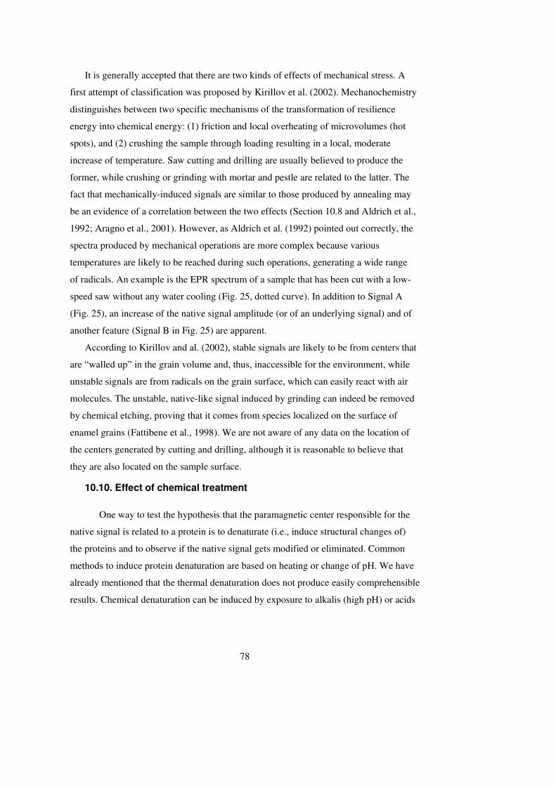
78

It is generally accepted that there are two kinds of effects of mechanical stress. A

first attempt of classification was proposed by Kirillov et al. (2002). Mechanochemistry

distinguishes between two specific mechanisms of the transformation of resilience

energy into chemical energy: (1) friction and local overheating of microvolumes (hot

spots), and (2) crushing the sample through loading resulting in a local, moderate

increase of temperature. Saw cutting and drilling are usually believed to produce the

former, while crushing or grinding with mortar and pestle are related to the latter. The

fact that mechanically-induced signals are similar to those produced by annealing may

be an evidence of a correlation between the two effects (Section 10.8 and Aldrich et al.,

1992; Aragno et al., 2001). However, as Aldrich et al. (1992) pointed out correctly, the

spectra produced by mechanical operations are more complex because various

temperatures are likely to be reached during such operations, generating a wide range

of radicals. An example is the EPR spectrum of a sample that has been cut with a low-

speed saw without any water cooling (Fig. 25, dotted curve). In addition to Signal A

(Fig. 25), an increase of the native signal amplitude (or of an underlying signal) and of

another feature (Signal B in Fig. 25) are apparent.

According to Kirillov and al. (2002), stable signals are likely to be from centers that

are “walled up” in the grain volume and, thus, inaccessible for the environment, while

unstable signals are from radicals on the grain surface, which can easily react with air

molecules. The unstable, native-like signal induced by grinding can indeed be removed

by chemical etching, proving that it comes from species localized on the surface of

enamel grains (Fattibene et al., 1998). We are not aware of any data on the location of

the centers generated by cutting and drilling, although it is reasonable to believe that

they are also located on the sample surface.

10.10. Effect of chemical treatment

One way to test the hypothesis that the paramagnetic center responsible for the

native signal is related to a protein is to denaturate (i.e., induce structural changes of)

the proteins and to observe if the native signal gets modified or eliminated. Common

methods to induce protein denaturation are based on heating or change of pH. We have

already mentioned that the thermal denaturation does not produce easily comprehensible

results. Chemical denaturation can be induced by exposure to alkalis (high pH) or acids

79

(low pH). Very high concentrations of alkalis or acids result eventually in the hydrolysis

of the peptide bonds (Driessens and Verbeeck, 1990). Enzymatic deproteination is

expected to keep the mineral component intact, and it could be a method to investigate.

Much can be learnt from the methods of protein denaturation in bones, where

standardized techniques are available (Anderson, 1982). One of them employs

extraction with (70- 90)% ethylenediamine (in H2O) in a Soxhlet refluxing apparatus at

116.5 °C. This technique effectively eliminates the native signal from the spectra of

bones and dentine (Wieser et al., 1994; Haskell et al., 1995). However, this treatment

has been found to induce apatitic recrystallization in bone minerals and conversion of

the amorphous phase to crystalline mineral (Termine and Posner, 1967). We are aware

of only one paper describing the effect of ethylenediamine on the native signal in

enamel (Romanyukha et al., 1994), which mentions an unsuccessful attempt of

application. Another method (Termine et al., 1973) uses 95% hydrazine at (40-60) °C.

Ivannikov et al. (2001b) proved this to be very successful in enamel: the signal

practically disappeared for grain sizes below 200 µm. Ivannikov et al. (2001b)

explained the success by the ability of the small molecules of hydrazine to penetrate

between the densely packed enamel prisms. However, an IR analysis performed on the

same treated enamel samples showed no changes in the amide bands (corresponding to

the absorption of the peptide bond) associated with the protein component, so that no

association could be made between the native signal and the proteins. Unfortunately,

this experiment has never been reproduced by other scientists, perhaps because

hydrazine is classified as toxic in many countries and its use is strictly regulated.

Deproteination methods based on the use of alkaline solutions have been known

for a long time. Alkaline denaturation with highly concentrated solutions (over 5 M) of

KOH has been shown to reduce the intensity of the native signal by about 50%

(Romanyukha et al., 1994; Fattibene et al., 2005). In contrast, high concentrations of

another alkaline, NaOH, are ineffective in the reduction/elimination of the native signal.

The correlation between the native signal and the proteinic component was

investigated by a comparative IR, Raman and EPR analysis of KOH- and NaOH-treated

enamel samples (Fattibene et al., 2005). IR and Raman observations showed

disappearance of amide bands after both alkaline treatments, indicating an almost

complete breakdown of the protein component. On the contrary, EPR measurements of

80

the same samples showed partial (for KOH) or no (for NaOH) elimination of the native

signal. So, once again (Ivannikov et al., 2001b), the native signal intensity and the

protein bands in the IR spectrum did not seem to be correlated. This was interpreted as a

proof that the precursors of the native signal are located not on a protein, but, more

likely, on a different organic molecule in the mineral component or at the interface

between the two, as illustrated more extensively in the next section. These findings have

lead only to a partial understanding of the origin of the native signal.

The described methods have indeed succeeded in the pragmatic goal of reducing

the native signal intensity. However, this is not a complete solution of the problem.

Although the 50% suppression of the native signal undoubtedly makes the evaluation of

the dosimetric signal easier, it is not quite clear yet that it does not affect the radiation

sensitivity, as we will see in the next section.

10.11. The mineral-organic system

Some studies of the origin of the native signal have revealed that there is a close

interaction between the mineral and the organic matrix. Starting from the widely

accepted assumption that amenoblasts initiate crystallization in calcified tissues and

that secreted proteins act as scaffolds for crystal growth (Fincham and Simmer, 1997,

and Chapter 3), some authors (Bachmann and Ellis, 1965; Termine et al., 1967; Marino

and Becker, 1967; Houben, 1971; Roufosse et al., 1976; Peckauskas and Pullman,

1978a; Kenner et al., 1998) proposed that the protein and the mineral components of

calcified tissues should be considered not as separate phases, but as an ensemble,

where proteins and mineral crystals are chemically bonded. A direct evidence of the

interaction of the COOH terminal region of amelogenin with the apatite crystal has

been provided (Shaw et al., 2004 and references therein). A hypothesis has been

proposed that, at the protein-mineral interface, the organic and mineral components

share molecules, most likely of carbon dioxide, which occurs in both hydroxyapatite

and amino acids. Therefore, tooth enamel should be modelled as made up of three

phases: a bulk mineral, a bulk organic, and a protein-mineral interface. This model is in

line with that proposed by Brik et al. (2000b), who surmised that the organic

component consists of two subsystems, which they called “Organic 1” and “Organic

2”. The first subsystem fills the space between the enamel prisms and is 10-20 nm

81

thick (perhaps corresponding to the bulk organic described above). The second

subsystem covers the hydroxyapatite nanocrystals and is 2-5 nm thick (the above

protein-mineral interface). Thus, the volume of “Organic 1” is much bigger than the

volume of “Organic 2”. It was also proposed in the same model (Brik and Brik, 1998)

to classify the biominerals as mineral organic nano-associated (MONA) systems. Much

experimental evidence for the existence of this interface region has been provided,

mainly on the basis of EPR (in dentine: Pass et al., 1990; Peckauskas and Pullman,

1978a; Roufosse et al., 1976; Houben, 1971; Termine et al., 1967; Kenner et al., 1998;

in bone: Becker and Marino, 1966). Fluorescence and luminescence measurements in

bone also contributed to these studies (Godfrey-Smith and Pass, 1997; Bachmann and

Ellis, 1965).

Now, another important question arises: Is the radiation sensitivity of the CO2-

precursors affected by the presence of the organic matrix in general and/or of the

centers responsible for the native signal, in particular? If the existence of a mineral-

organic matrix interface is accepted, it would not be surprising that the radiation

sensitivity of the CO2- precursors is affected by the presence of the organic matrix. It is

quite reasonable to assume that the CO2- radical is located on the “surface” (Chapter 9).

From a more general physical viewpoint (which will be discussed in detail in the next

chapter), there should be an effect when precursor centers in the organic or interface

region can compete for the same radiation-induced carriers (electrons, holes) in the

mineral. Fattibene et al. (2006) and Kenner et al. (1998) reported that the dosimetric

signal intensity per unit dose (i.e., radiation sensitivity) is higher for deproteinated than

for intact dentin by a factor larger than 2. A possible interpretation of such increase is

that the organic component acts as a scavenger and assists recombination of carbonate

free radicals induced by ionizing radiation. That was also suggested by Peckauskas and

Pullman (1978a), albeit in a different experiment. According to Kenner et al. (1998),

the observed radiation-sensitivity increase in dentine also confirms that the pre-centers

responsible for the dosimetric signal are partly located on the surface of the crystals,

exposed to the organic component. A similar mechanism could be assumed to occur in

enamel, but no radiation sensitivity increase has ever been reported in deproteinated

enamel. It cannot be ruled out, however, that the radiation sensitivity does change, but

it is very difficult to prove in enamel for at least two reasons. First, it is because the

82

organic content of enamel is small and deproteination could only weakly affect the

radiogenic signal. Second, in view of the extreme resemblance between the different

types of CO2- signals (Chapter 9), even a substantial reduction of one type would not

be easily detectable from a line shape change in a powder spectrum. Enamel plates and

relatively high doses will be required to investigate the potential effects in detail.

10.12. The native signal as a bioindicator of tooth health status

Brik et al. (2001a) pointed out that the radicals responsible for the native signal are

related to broken chemical bonds and, therefore, a large number of these radicals may

be an indicator of pathological processes in mineralized tissues. Indeed, the native

signal from caries teeth is stronger than from healthy ones (Brik et al., 2001a; Sholom

et al., 2000b).

Sholom et al. (2000b) reported that treatment with KOH decreased the native

signal in carious parts of teeth to its level in the healthy fractions of the same teeth.

Similarly, Romanyukha et al. (1999a) showed that the KOH treatment reduces the

native signal more effectively in diseased teeth than in healthy ones. This can be

explained by the lower degree of mineralization in carious teeth. Kuhar et al. (1997)

have demonstrated that diffusion of molecules through hard dental tissues is higher in

teeth demineralized by acid etching. It is reasonable to assume that this applies also to

teeth with cariogenic demineralization. We emphasize that Romanyukha et al. (1999a)

found this effect not only in carious teeth, but also in teeth affected by periodontal

disease, a disease of the gum. They suggested that the native signal can be used as a

biomarker of more general pathological processes.

On the other hand, a correlation between a disease or aging and the native

signal from bone tissues has not been proved conclusively. For example, Kenner et al.

(2005) found that the intensity of the native signal in bone decreased in HIV and

uncontrolled diabetic patients.

10.13. Origin of the native signal: a still unanswered question

If one wants to eliminate or substantially reduce the native signal by a treatment

(preferably without affecting the dosimetric signal), it is desirable to know the identity

of the radicals responsible for it. It was suspected from the outset (Ikeya et al., 1984;

Tatsumi-Miyajima, 1987) that the organic part of the enamel played an important role in

83

the origin of the native signal. As discussed in the previous sections of this chapter, a

signal resembling the native signal of tooth enamel has been found in spectra of many

various biological and non-biological tissues. For instance, a paper by Brik et al.

(2001a) reported native-like signals in tooth enamel, dentine, femur bones of cow and

rat, collagen from rat tail and irradiated gelatine, and even in synthetic hydroxyapatite

commonly used for bone implants. In the latter case, the original hydroxyapatite

supposedly contains no organic matter and, indeed, it did not show native signal. The

same hydroxyapatite extracted from bone implant exhibited a native-like signal

approximately ten times stronger than the signal in the normal bone. A plausible

explanation is that the number of radicals is higher in the proteins that penetrate into the

implanted hydroxyapatite (and promote the bone growth) than in bone.

However, it seems that no significant progress has been made in the past

decades in accurate microscopic identification of the responsible radicals, and a

convincing identification of the radicals will probably be hard to perform, if not

impossible. The problem is that, essentially, only one g-value is known and no

additional information can be obtained from the line width. EPR alone is rather

powerless in such situations, and assistance of other methods will be indispensable.

There are some alternative interpretations, which should not be rejected

outright. The similarity between the native signal of tooth enamel and the signals of the

other aforementioned tissues, on the one hand, and the signal produced by semiquinone

radicals, on the other, is noteworthy. For instance, the EPR spectrum of hair has a

signal in the g-value range of 2.0036-2.0046 (depending on the hair color), whose line

width is 0.8 mT (Kudynski et al., 1994). This signal is currently assigned to melanin,

whose basic structural units are molecules of compounds of the quinone class (Riley,

1997). Based on the similarity between the semiquinone and the native signal in bone,

Kenner et al. (2005) have performed some experiments demonstrating that at least one

of the signals composing the native signal in bone is due to semiquinone radicals.

Semiquinones are effective radical scavengers; they could neutralize radiation-induced

carbonate radicals, and, thus, influence the radiation response of tooth enamel. (Section

10.11).

In Fig. 26, four spectra of entirely different origins are compared (from fossil

tooth enamel (a), from frog leg (b), from unirradiated tooth enamel (c), and from

84

synthetic apatite (d)). They saturate at very different powers: apatite signal (perhaps

from a surface CO- radical, see Moens et al., 1991, 1993a) at 0.5 mW, the native signal

from enamel at 2-5 mW (Ignatiev et al., 1996), while the signals from frog leg and

fossil teeth at 5-10 mW. Still, all of them saturate at lower powers than the radiation-

induced (CO2-) signal (above 10 mW). We studied the low-field signals shown in Fig.

26 (no other signals are visible in Fig. 26c) from synthetic apatites, frog legs and fossil

enamel and found them clearly radiation-sensitive. That was also found in some studies

of the native signal in tooth enamel (see Section 10.4).

Although the low-field components in the spectra of Fig. 26 look very similar,

it would be surprising to find that these signals are all due to the same radical.

Moreover, the spectra may be composite in some cases. Also, the g-tensors are not

necessarily isotropic (see, e.g., the three different principal g values for CO-).

The spectra in Fig. 26 are, in our opinion, very indicative of a particular

problem. How can one be sure when comparing spectra obtained from, say, human and

bovine enamel, or enamel and bone, or enamel heated at 100 °C and at 300 °C, that

the two spectra contain the same EPR components? If this cannot be demonstrated, one

should be careful with statements like “the native signal is increasing with heating”. As

illustrated above, g shifts and variations in line width are very common, and this means

that either other radicals are involved or the environment of the same radicals is

different. All this adds to the individual variability, which was discussed in a previous

section. Contributions from CO- could at least partially account for some of the signals.

There are other possibilities. Thus, it is dangerous to ascribe a completely organic

origin to the native signal.

Some scientists think that understanding the origin of the native signal will be a

panacea for all the problems still remaining in tooth enamel dosimetry. Even if not

quite so, it will certainly result in dramatic improvements of the method and reduction

of uncertainty in dose estimates. Once the centers responsible for the native signal are

known, it will be easier to find a correct way to eliminate them. In the meantime, tooth

enamel dosimetry has to live with the native signal, and we can only try to find out as

many properties of the involved signals as possible.

10.14. Impurity signals

85

Another type of radiation-unrelated signals is so-called parasitic signals. These signals

show up in tooth enamel spectra randomly, and their origin is as obscure as the origin of

the native signal. They are generally attributed to unidentified impurities in the crystal.

Little attention has been paid to such signals, although, in some samples (fortunately,

only very few), they completely mask the dosimetric signal and render the sample

useless for dosimetric purposes.

Fig. 27 shows three examples of typical parasitic signals. Fortunately, Spectrum

(a) is fairly rare, but the signals indicated by arrows in Spectra (b) and (c) appear in the

majority of samples. A sample producing a spectrum like Spectrum (a) should

obviously be simply rejected, but, with Spectra (b) and (c), one may wonder if the

parasitic signal amplitude could be reduced to a less harmful level by an optimal choice

of EPR acquisition parameters. That seems unlikely because they saturate

approximately at the same power as the dosimetric signal (Skvortsov et al., 1995). They

can partially be eliminated by a purification treatment (Chapter 12), although there is

always some risk of introducing other impurities or paramagnetic centers in such a

procedure (Section 10.10). As for the origin of these signals, it is not clear whether they

are intrinsic to the enamel or introduced in the sample preparation. For example,

Kirillov et al. (2002) showed that using diamond tools in preparing samples may

introduce signals similar to those of Spectrum (c) in Fig. 27. Shishkina et al. (2001b)

suggested that metal ions transferred to saliva from tooth fillings are responsible for

these lines, although similar signals have been observed in fossil samples as well. Also,

some chemicals contain large amounts of metals, which could contaminate samples

during the preparation. Again, EPR alone is unlikely to give a definitive answer

regarding the origin of these signals, and comparative studies with other methods should

be undertaken.

The presence of transition metal ions, such as Mn2+ and Cr3+, has been investigated by

Brik et al. (2001b), who have found Mn2+ signal in the CaCO3 phase of tooth enamel

(for a multiphase model in the mineral of tooth enamel, see Driessens and Verbeeck,

1990, p.130-136). The intensity of the Mn2+ signal changes with heating and γ-

irradiation. No Cr3+ has been found by Brik et al. (2001b), whereas Doi et al. (1981b)

reported a Cr3+ signal in heated tissue. The presence of Mn2+ in the spectrum has

86

important practical consequences, as it makes using external Mn2+ reference samples

less reliable (Chapter 13).

11. Linearity/nonlinearity of the dose response: Is there a need

for solid-state modelling of the radiation-induced

processes?

The previous chapters have shown that EPR tooth dosimetry still has many unanswered

questions, such as whether the native signal is really radiation-insensitive, whether there

any unknown problems in determining doses above 500 mGy and whether the EPR

response of tooth enamel is really linear. The main purpose of this chapter is to discuss

a number of aspects of the solid state that could help in finding answers to them. Some

of these issues are very complex, and extensive experimental and theoretical research

will be needed to clarify their potential role in EPR tooth dosimetry.

Tooth enamel is a complex material (Chapter 3), but, in interpreting dose

response curves, it is usually regarded as a homogeneous mineral phase with typical

solid state properties. Many complex processes could occur during and after irradiation

even if the system was a “simple single crystal”. The following description, albeit

simplified and mainly qualitative, will provide tools and offer new perspectives to

address some of the remaining problems.

When radiation of sufficient energy, hν, interacts with a solid, charged particles

(electronic, ionic, molecular, radical) are formed in the energy dissipation process. Once

formed, they may get attached; however, oftentimes they are very mobile, especially

electrons and holes (missing electrons). An electron and a hole (or two radicals) may

recombine, or they may get trapped temporarily somewhere in the system. Eventually,

this produces stable, trapped radicals and defects. Some of these states are detectable by

EPR, but others are not.

Some paramagnetic defects are formed very fast (within 1 ns), whereas

formation of others comprises slow ionic and electronic processes, which take hours and

even days. Such processes (e.g., generation, diffusion, trapping, recombination,

87

destruction) can be described mathematically and modelled. In some cases, reasonable

qualitative and quantitative agreement with results of experimental studies was found

(e.g., Bube, 1992, Chapter 2; Grün, 1994; Jonas and Marseglia, 1997; Hua et al.,

2000a,b; Nelson, 2005 and references therein). The main components of such models

are generation rates and concentrations of free carriers, traps and recombination centers,

as well as cross sections of such processes as trapping and recombination. The concept

most important for tooth enamel dosimetry is the competition between different

processes or reactions that may occur in models comprising more than one type of

trapping and/or recombination centers.

A band structure model is one of the approaches to describe an insulating

material, like hydroxyapatite, interacting with ionizing radiation (see, e.g., Kittel, 1996,

Chapter 7). Although this model contains all necessary elements, one should be aware

that it is only a semi-empirical approximation involving many assumptions and

parameters.

Interaction of radiation of sufficient energy with a hydroxyapatite crystallite

sample will create free electrons and free holes in the conduction band (CB) and valence

band (VB), respectively. These bands extend over the whole crystal (long lines in Fig.

28; the upper long line denotes the bottom of the CB; the lower line shows the top of the

VB). They originate from the lowest unoccupied (CB) and highest occupied electronic

levels (VB) of the individual atoms or ions constituting the solid. The difference

between the bottom of the CB and the top of the VB constitutes the so-called band gap,

which is in the range of 4.5 – 5.3 eV (Calderin et al., 2003). The energy of the energy

quantum, hν, capable of generating the aforementioned free charge carriers corresponds

roughly to a wave length of 250 nm.

Minerals, like apatite, contain numerous defects. In many cases, they have a

profound effect on macroscopic properties of the mineral. These defects can be intrinsic

(e.g., vacancies, interstitials) or extrinsic (impurities). They may trap electrons or holes

or act as recombination centers. In hydroxyapatite, Ca2+ vacancies and CO32- ions can

be considered (Driessens and Verbeeck, 1990). The exact behavior of a defect depends,

in particular, on the temperature, the dose rate and the details of the structure of the

defect. To indicate the localized nature of such defects, their energy levels are

represented by short lines in Fig. 28.

88

Some of the traps may have an unpaired electron prior to irradiation and become

diamagnetic after it, whereas other defects do not trap anything and are not affected by

radiation at all. The traps most important in the present context become paramagnetic

during and after the irradiation. For example:

2 33 3

233

CO e CO ;

CO h CO

− − −+ →

− + −+ →

(11.1)

In these trapping processes, 2CO3− is the diamagnetic precursor; it serves as an electron

trap in the former process and as a hole trap in the latter. Whether 2CO3− traps an

electron or a hole depends on small differences in its environment (like presence of a

Ca2+ vacancy or an impurity ion). As a consequence, a simple notation of 2CO3− is not

sufficient. The two trapping events have been found in both tooth enamel and apatites

by EPR (Chapter 8). However, electrons and/or holes can also be trapped without

giving rise to a paramagnetic defect or produce paramagnetic centers undetectable by

EPR at room temperature due to the specific relaxation properties of the latter (Chapter

4). This means that some electrons and holes generated by irradiation are invisible for

EPR. These basic, but relevant examples illustrate that the relationship between the

absorbed dose and the amplitude (intensity) of the associated EPR signals is not simple.

It is clear in the formation process described above that the number of, say,

CO3− centers cannot exceed the number of 2CO3

− precursors, regardless of the dose.

Therefore, the EPR signal will not increase infinitely, but will saturate at a certain,

possibly very high dose. (After that, even a signal decrease is possible due to

destruction of precursor centers; see, e.g., Nelson, 2005.) Such growth curves are often

described by a saturating exponential function (see, e.g., Grün 1994):

1−= − D / Dsatn N( e ) , (11.2)

where n is the number of trapped electrons or holes (m-3, proportional to the EPR

signal), D is the dose, N is the number of traps (the maximum number of electrons or

holes that can be “accommodated” by this trap, m-3); and Dsat is the characteristic

saturation dose, inversely proportional to N and the cross section of trapping S (m2). The

cross section depends, in particular, on the size of the trapping defect and its charge. It

89

varies over several orders of magnitude, from 10-16 to 10-26 m2; the value 10-19 m2 is

found most often, which corresponds roughly to the surface area of an atom (Bube,

1992, Chapter 6). When present in equal concentrations, traps with a larger S (smaller

Dsat) get filled first.

Some insight into the system can be gained by comparing the number of

electrons or holes generated by a certain dose with the number of available traps. At

low doses, the former may be insufficient to saturate all traps. As the dose increases

and the number of generated electrons/holes becomes much larger than the number of

traps, the excessive electrons or holes have to go somewhere else, for example, to

another trap available in a higher concentration, to a recombination center, or into areas

outside the solid (possibly organic phase or surface). When several types of traps and

recombination centers are present simultaneously (as is undoubtedly the case in human

tooth enamel), these centers compete with each other. The outcome (distribution of

electrons and holes over the traps) depends on many parameters, such as trap

concentration, dose rate, irradiation time, and temperature in a complex way.

In order to give some feeling of what the competition could mean, we consider a

system with just two permanent electron traps. The concentration of Trap 1 is high, say,

100 times the concentration of Trap 2 (N1 = 100 N2). Both traps give rise to a

paramagnetic signal (assuming further that equal numbers of trapped electrons produce

the same EPR intensities for Traps 1 and 2). Along with the number (concentration) of

traps, the cross section may also play an important role. It is clear from Eq. (11.2) that,

if the cross section of Trap 2 is smaller than the cross section of Trap 1, the contribution

from Trap 2 to the total EPR spectrum will be at least 100 times smaller than the

contribution from Trap 1, and, in practice, Trap 2 can be neglected.

However, when the cross section of Trap 2 is considerably (say, 1000 times)

larger than the cross section of Trap 1, an interesting competition process may occur.

At low doses, Trap 2 will trap electrons more effectively than Trap 1, and the EPR

signal from Trap 2 may be larger than the EPR Signal from Trap 1 despite its lower

concentration. Trap 1 will capture fewer electrons than in the case where Trap 2 is

absent. Nevertheless, when the dose becomes high enough (the exact value depending

on the relative values of the trap concentrations and cross sections), Trap 1 will start






Met opmaak: Engels

(Groot-Brittannië)

Verwijderd: (11.2)

90

dominating Trap 2, and, eventually, the total EPR signal will originate solely from Trap

1 (see Fig. 29, supralinearity).

It is also important for our purposes to know the stability of the newly-formed

paramagnetic centers and possible mechanisms of their decay. A paramagnetic center

may decay (either becoming invisible to EPR or transforming into another paramagnetic

defect) in three essentially different ways:

1) the trapped electron (hole) may get thermally or optically excited, move to the

CB (VB) and become retrapped by the same or another, more stable, center;

2) the electronic carrier may remain localized on the impurity while a part of the

defect (vacancy) drifts away giving rise to a center of another type;

3) the trapped electron may recombine at the site of its location with a free hole, or

vice versa.

These simple considerations illustrate that a part of the dose effect (generated electrons

and holes) may get lost in several ways. Neglecting the effect of recombination centers

to some extent, we can draw a few simple conclusions:

1) Using the intensity of the EPR signal of one paramagnetic center (e.g., CO2-)

may lead to different results than using the intensity of another signal (e.g., CO3-

). That may happen, for example, if precursors of one type get saturated at a

lower dose than precursors of the other. By the same token, using the total

intensity of signals of all paramagnetic centers may produce yet another result.

2) Despite the presence of competing traps (e.g., traps occurring in a lower

concentration), stable trapping at an abundantly present trap (with a sufficiently

large cross section) may lead to an EPR contribution that dominates the global

EPR spectrum at high dose (this is likely to be the case for CO2-).

3) Even if a constant dose rate is assumed, a particular EPR signal does not always

grow linearly with the dose.

4) Competition between traps is stronger at lower doses. At higher doses, several

types of traps may have been eliminated by saturation, that is, are permanently

filled. This implies that detailed knowledge of the processes described above is

especially important when low dose values are assessed. However, essential

information on the ionic, electronic and optical properties of apatites and their

impurities is still lacking. A somewhat simplified calculation shows that, for a

91

band gap of approximately 5 eV, doses in the 0.1 - 1 Gy range may result in free

electron/hole concentrations comparable with those of dopants present in the

ppm-to-percent range. Therefore, the latter may (or may not, depending on their

cross sections) influence the low-dose behavior of the EPR signal.

Consequences for the linearity of the dose response

Thus far, our considerations were qualitative. We will now make some

quantitative predictions about their effects on the dose response curve. It would be ideal

to have a linear relationship between the intensity of an EPR signal I and the dose D:

I ~ D or

I = aD. (11.3)

In most studies, such linear relationship was assumed for a fairly wide range, up to the

kGy doses, regardless of the method applied to evaluate the EPR intensity (Liidja and

Wieser, 2002; Desrosiers and Schauer, 2001). Saturation effects have been reported

only at doses beyond those of interest for retrospective dosimetry. It is worth noting

that Grün argues that linear fitting should be completely abandoned in dating studies, in

spite of the presence of “apparent linearity” in the ranges far below saturation (Grün

1996, 2006a). It seems reasonable to assume that, in retrospective dosimetry, deviation

from linearity at the high-dose end is less likely than in dating.

However, deviations from (apparent) linearity can also occur in the very low

dose range (far below saturation) (supralinearity, see above and Fig. 29). As soon as

more than one trapping or recombination center are involved, problems with the

linearity of the dose response can be expected, as was discussed, for example, by

Romanyukha et al. (2005). Assuming the (quite plausible) existence of more than one

type of CO2- radicals and a (more arguable) dose dependence of the following form:

I = I1(1-exp(-D/Dsat)) + kD, (11.4)

the authors demonstrated the possibility of overestimating the dose and proposed this as

a possible explanation of the problem of the so-called “intrinsic dose” or “predose”.

They essentially considered a surface CO2- radical with a saturation dose Dsat of 200

mGy and a high-concentration bulk CO2- radical. Within the restrictions of this

example, a predose of 180 mGy (instead of 0) resulted from the apparent (but not real)

92

linear dose behavior that would have been measured in practice. Also, Jonas and

Marseglia (1997) concluded that traps with different filling behaviors can easily lead to

incorrect dose estimations. These authors used a quasi-classical theory describing the

electrons as localized pseudo-particles rather than delocalized charges in a band

structure model.

To conclude this chapter, we return to the phenomenon of supralinearity, which

may be relevant to EPR tooth dosimetry. It is important for low-dose dosimetry to

evaluate whether there is a dose range with a smaller trapping efficiency (supralinearity)

or even zero slope (Fig. 29). Theoretically, this is certainly possible when either the

concentration or the cross section of (a) competing defect(s) (2 in Fig. 29) is not

negligible in comparison with the corresponding characteristics of the dominant

defect(s) (1 in Fig. 29, CO2- ?). If such a region is present, it will lead to an

underestimation of the dose, as is obvious from Fig. 29.

As illustrated by the two-trap example above, supralinearity is due to

competition between traps. The extracted signal, the intensity of which is plotted (e.g.,

in Fig. 29), is, in principle, due to only a single type of CO2- radical (1). The

contributions from the competing radicals to the global EPR signal are supposed to be

eliminated by successful spectrum decomposition. This is, of course, automatically

fulfilled when the competitive trap produces EPR-silent centers, because they do not

contribute to the total signal. If a second trap consumes a major part of the electronic

carriers in the low-dose range, the signal of the major CO2- radical will be reduced.

Obviously, this cannot last long with increasing dose because the number of generated

electronic carriers will eventually become so large that it will exceed by far the (small)

number of available traps of the second type. Beyond that dose, the effect of Trap 2 on

the formation of CO2- will become negligible.

The problem is that it is very difficult to identify supralinearity experimentally

because of the unknown model parameters (trap concentration, cross section) and the

large uncertainties in signal measurements in that range. The precursor of the native

signal may be such a strongly competing trap that it gets saturated at a very low dose.

This could explain the weak dose dependence of the native signal that has sometimes

been reported. Other competing traps could be impurities like those shown in Fig. 27.

93

We realize that this chapter contains a lot of speculation about the behavior of

the traps (Trap 1, presumably associated with the formation of CO2-, and the competing

Trap 2) as a function of dose. Important issues that need to be resolved are the

mechanism of formation of CO2- (which may run not in the way suggested by Eq. (9.1))

and the related issue of the identity of its precursor. Nonetheless, we feel that enough

arguments have been presented to make the reader aware that certain things in tooth

dosimetry (in particular the dose-response curve) may not be as simple as they look. It

is clear that extensive computational studies based on relevant models are necessary to

verify the statements made above. Examples of such studies performed, for example, in

EPR dating, can be found in the literature cited in this chapter and the references

therein.

12. Sample preparation

12.1. Introduction

Samples are prepared so as to obtain dentin-free powder of pure enamel. There is no

standard, commonly accepted procedure for sample preparation yet, but the majority of

the methods currently in use comprise the same sequence of steps:

1) tooth sterilization and storage;

2) separation of the crown from the root;

3) separation of enamel from the dentin;

4) enamel grinding;

5) enamel purification.

As it should be clear now from Chapter 10, each of these steps may exert unwanted

effects, such as a change in the crystal structure, generation of paramagnetic centers, or

contamination. We have shown in Chapter 11 how these effects can influence the dose

response in principle, and, in the subsequent chapters, we will review the effects of

sample preparation on dose response reported in the literature. This chapter will focus

mostly on the technical aspects of sample preparation.

12.2. Tooth storage and decontamination

94

One of the first questions that a dosimetrist faces when planning an EPR dose

reconstruction is how to handle a tooth. The most frequently asked questions are

whether it is hazardous to health, whether it has to be treated as a potentially infectious

human tissue, and how it should be disposed of. People worry mostly about viruses like

HIV or HCV. It is advisable to collect information relevant to regulations in a specific

country in advance. Basic guidelines, however, are more or less universal, and some

general recommendations can be given here. The USA agencies Center for Disease

Control (www.CDC.gov) and Occupational Safety and Health Administration

(www.OSHA.gov) have provided helpful guidelines on decontamination of extracted

teeth to be used as diagnostic specimens or dental educational tools. Here, we provide a

summary of these recommendations.

The first important point is that it is attached tissues or blood that make the tooth

hazardous. Extracted uncleaned teeth must be presumed infectious and must be handled

and wasted like biohazardous materials. By contrast, sterilized and powdered enamel is a

dry and stable mineral substance, which cannot be regarded as a biological material. For

safe delivery from a dentistry clinic to an EPR laboratory, the extracted tooth should be

placed in a leakproof container and labeled as biohazard. Teeth are usually still

uncleaned upon arrival at the EPR laboratory. They should not be stored in such

condition for too long; storage in room-temperature water should be particularly avoided

because it favors bacterial growth. Sterilization should be performed with a chemical

disinfectant of at least medium-level activity (also known as tuberculocidal claim

activity), which will kill lipid medium-sized viruses, like hepatitis or HIV, as well. An

appropriate chemical would be the ordinary household bleach (sodium hypochlorite,

5.25% or 6%) diluted ten-fold with tap water (treatment for 24 h), or formalin, which

contains formaldehyde.

The question of primary importance for dosimetry is whether the changes

induced in the tooth tissues by such safety procedures can alter the EPR dose response.

The available literature data on the effects of storage and sterilization media on the

properties of tooth tissues are much more useful for orthodontists than for EPR

dosimetrists (Kuhar et al., 1999 ; Petelin et al., 1999). There is evidence that other

sterilization methods, such as autoclave or dry heat, can modify the mineral component

of teeth, which could affect EPR measurements (DeWald, 1997). Hydrogen peroxide

95

should be avoided because of the obvious potential oxidation effects. Inexplicably, the

effect of sterilization procedures on EPR properties of enamel has been given little

attention, as Bhat (2005) has also pointed out. This preparation step is seldom described

in the EPR dosimetry literature.

After sterilization, the teeth must be rinsed and stored until further preparation.

The official protocols mentioned above recommend that the tooth be stored in water after

sterilization to prevent its cracking. However, it is not known whether the wetness of the

tooth is important for the subsequent preparation for EPR measurements (Bhat, 2005).

As stated above, cleaned teeth are not regarded as a potentially infectious

material, and, consequently, they do not have to be declared as biological samples to the

international express mail companies.

Another common question about transportation concerns the dose received by

tooth samples when they are x-rayed at the airports or shipped by air couriers. Tanaka et

al. (2006) investigated the effect of airport x-ray baggage scanning on tooth dose and

found that the difference between the estimated dose of scanned and non-scanned

samples was smaller than the experimental uncertainty. Based on these results, they

concluded that the dose from x-raying is negligible for EPR dosimetry.

12.3. Separation of crown from root

The second step is to separate the crown from the root (enamel is present only in

the crown). Most of the procedures proposed in the literature use a power-driven

diamond or steel-wheel saw. Kirillov et al. (2002) have warned about possible

contamination of the enamel by diamond tools (see also Section 10.14). Attention must

be also paid to cooling the sample with water in order to avoid overheating due to the

friction between the wheel and the crown (Aragno et al., 2001; Kirillov et al., 2002;

Sections 10.6 and 10.7).

The crown is then cut in two parts. Dividing a tooth into buccal and lingual

halves makes it possible to reveal differences in the doses due to x-ray dental exposures

(see, e.g., Chumak et al., 2006). Alternatively, the tooth can be divided into medial and

distal parts (Chapter 3), which will average the doses to the parts exposed and

unexposed to x-rays (this aspect will be dealt with more extensively in the following

chapters). It is a common practice to divide incisors into lingual and labial parts, as the

96

effect of the solar light on the native and the dosimetric signals has not been wholly

elucidated yet (Chapters 10 and 17).

12.4. Separation of enamel from dentin

The goal of enamel sample preparation is essentially to produce samples of pure

enamel, completely free of dentin. An experiment performed by Wieser et al. (2001)

suggests that residues of dentin in the enamel sample can bias the EPR-reconstructed

dose. They prepared two sets of samples using two variants of the same protocol based

on a sodium hydroxide treatment. In one case, the whole crown was immersed in a

sodium hydroxide solution (Method A), whereas, in the other case, the crown was cut

in half to facilitate access of sodium hydroxide to the dentine (Method B). The samples

prepared by Method B resulted in 10% higher radiosensitivity and lower variability of

EPR measurements. This difference was explained by possible residues of dentine in the

samples prepared by Method A. Although one could question the statistical significance

of these numbers, the result is quite reasonable, as dentin and enamel have different

organic/mineral compositions and different radio-sensitivities.

The methods currently used to separate enamel from dentin can be

conventionally classified as mechanical and chemical. Mechanical methods make use

of common orthodontic tools, such as drills (see, e.g., Ivannikov et al., 2004; Rossi et

al., 2000; Trompier et al., 2006). As has been widely discussed, precautions should be

taken not to overheat the sample (Desrosiers et al., 1989; Aragno et al., 2001; Kirillov et

al., 2002; and Sections 10.6 and 10.7). For this reason, some EPR dosimetrists prefer to

crush the tooth in big pieces with mortar and pestle (see, e.g., Romanyukha et al., 2000).

In chemical methods, reagents are used to remove dentin from enamel. Their

effect is based on the same principles as described in Section 10.8 in connection with

reduction of the native signal in tooth enamel. In this case, the goal is to break peptide

bonds in the proteins contained in dentin. Because of the high organic material content

(approximately 30% by weight), deproteination has the effect of softening a large part

of the dentin, which can be eventually separated from enamel by softly scratching.

Alkaline solutions are widely used to this end. Typical concentrations of aqueous

solutions of sodium hydroxide (NaOH) range between 5 M and 8 M (Romanyukha et

al., 1994; Nakamura and Miyazawa, 1997; Haskell et al., 1997; Wieser et al., 2001;

97

Chumak et al., 2006). Some authors (Romanyukha et al., 2000; Cieselski et al., 2006)

use KOH, which, as shown in Section 10.8, offers the double advantage of softening the

dentin and reducing the enamel native signal intensity (this advantage is not

unquestionable, though; see Sections 10.8 and 10.9). The procedure is more effective

when performed in an ultrasonic bath at 60-80 °C for 10-20 h (Romanyukha et al.,

2000), although it was also used without ultrasonic bath, in which case it took four

weeks to soften the dentin (Nakamura and Miyazawa, 1997). The ultrasound power is a

critical parameter because it strongly affects the effectiveness of the chemical attack.

Depending on the alkaline concentration, treatment duration, and characteristics of the

ultrasound bath, small residues of dentin may remain attached to enamel, which would

require subsequent drilling (in this case, the method becomes chemical-mechanical)

(Wieser et al., 2001; Vanhaelewyn et al., 2001; Egersdorfer et al., 1996). Other authors

do the opposite: first, they use a mechanical procedure to separate the dentin from

enamel and then treat enamel with an alkaline solution to complete dentin separation

(Ciesielski et al., 2006). Enamel and dentin can also be separated by gravitation

methods using a high-density liquid (e. g., sodium-polytungstate with the density of 3.1

g/cm3 ) (Brik et al., 1996; Sholom et al., 1998a).

It has been proposed to use fluorescence of dentin at 365 nm to detect residual

dentin spots on tooth enamel, but this method is not completely free of drawbacks

(Fattibene et al., 1998, and Section 10.5). The enamel can be also checked for dentin

residues with optical microscopy (Gualtieri et al., 2001).

When the dentin must be preserved for future measurements or for archival

purposes, chemical procedures are not appropriate because dentin undergoes a strong

attack, whose consequences are not very well known (Fattibene et al., 2006; Kenner et

al., 1998). In such cases, enamel and dentin are separated by mechanical tools

(Romanyukha et al., 2001). According to Ivannikov et al. (2004a), hard alloy drills are

harder than dentin and softer than enamel, and this property makes identification of the

enamel/dentin interface easier than with diamond drills.

12.5. Tooth enamel grinding

Once the enamel is separated from the dentin, it has to be reduced to small pieces in

order to be inserted in the measurement tubes or to be mounted on some sample holder.

98

In principle, enamel chips can be prepared by crushing the enamel with surgical pliers

or nippers (see, e.g., Trompier et al., 2006; Gualtieri et al., 2001; Serezhenkov et al.,

1992; Pass and Aldrich, 1985). That is usually done to prepare plates for the EPR and

ENDOR studies focused on signal anisotropy, like those described in Chapter 9. When

dose assessment is envisioned instead, samples are powdered to decrease the uncertainty

in signal amplitude readings resulted from anisotropy.

It was mentioned in Section 5.5.3 of this review that, in order to be ideally

isotropic, a powder must contain a large number of micro- or nanocrystals (well over

100). Mombourquette and Weil (1992) have estimated that the number of crystal

orientations necessary for achieving a high-precision powder distribution ranges from

106 to 108. If grains are of a regular shape, the number of grains per unit mass is

expected to decrease with the third power of the grain size. However, it was found

experimentally that the average numbers of grains in 100-mg samples of powders with

grain sizes in the ranges of 1-2, 0.5-1, and 0.1-0-5 mm are approximately 20, 100 and

1500, respectively. The deviation from the "third power law” is likely due to the

irregular shapes of the grains. From this viewpoint, the benefit of using 0.1-0.5-mm

grains is obvious. On the other hand, grinding down to grain sizes below 0.1 mm

increases the native signal and changes the dose response (again, see Section 10.7 and

the following chapters). Static electricity is also a practical problem when fine powder

is to be inserted in a measurement tube.

Grinding is usually done manually with a mortar and a pestle (ideally, agate in

order to reduce contamination). Grains of different sizes are separated by sieving.

Because of the irregular shape of the grains, their effective dimensions after sieving can

be larger than the sieve specifications (the grain can pass through the grid in an

orientation with its smallest side fitting the hole) (Fig. 30). Using electric grinding tools,

like those typically employed in bone grinding, has not been reported.

12.6. Tooth enamel purification

Some of the unintentionally induced signals described in Chapter 10 can be

eliminated by purification treatments.

It is advisable to store samples for some time between sample preparation and

EPR measurements in order to allow the unstable signals induced in sample preparation

99

to decay. An alternative and faster way to eliminate the transient signals is heating.

Chumak et al. (2006) routinely anneal ground samples in a ventilated oven at 90 °C for

2 h. Cieselski et al. (2006) heat samples at 150 °C for 90 min. However, the latter

group has also shown that this procedure may induce EPR signals in some samples, in

line with our overview in Section 10.6.

Unwanted stable paramagnetic centers can be removed by chemical

etching if they are located at the surface of the grains. In general, any acid

can be used for this purpose, but each one requires a specific protocol to

make its use effective. When an acid attacks the mineral, a barrier of crystals

is formed at the dissolution front, which blocks the effect of the acid on the

enamel (see, e.g., Chow and Brown, 1973). This barrier can be removed by

water. So, an etching procedure must include alternating steps of acid

etching and water rinsing. The rate at which such barrier is formed depends

nonlinearly on acid concentration and exposure duration (see, e. g., Fattibene

et al. 1998, for a protocol of etching with phosphoric acid). A limitation is

that strong acid etching cannot be applied to very fine powder, say, with

grains below 0.5 mm, because the grains would be practically lost. Etching

is also useful when parasitic signals originate from the enamel surface or

metal impurities deposited on it. A 5-minute immersion of enamel powder

in a 20% aqueous solution of acetic acid has been shown to remove the

former (El-Faramaway, 2005b), while EDTA (ethylenediaminetetraacetic

acid) in an ultrasonic bath or acetone is expected to remove the latter (this

has not been proven, though). It is perhaps noteworthy that taking impurities

off the tooth surface is the only operation reported for preparation of whole

intact teeth to be measured in L band (Zdravkova et al., 2003b) and

sometimes in X band (Wieser and El-Faramawy, 2002).

Etching with an acid is useful also because it shortens the lifetimes of the

unstable surface signals. For instance, the native-like signal induced by high-

wavelength UV (Section 10.5) decays approximately in one week under normal storage

conditions, but just a 24-h period is sufficient to reduce the unstable signal to a

negligible intensity if the sample has been in the phosphoric acid etching cycle

(Fattibene et al., 1998).

100

Enamel samples need to be thoroughly dried before EPR

measurements to avoid absorption of microwaves by water in the resonant

cavity. The methods used for drying are annealing for at least 10 h at (50 –

60) oC (see, e.g., Romanyukha et al., 2000c), drying in vacuum (< 5 kPa) at

40 °C for 30 min (Goksu et al., 2002), and storage for three days at room

temperature and relative humidity below 60%.

It should be mentioned that radiation also induces unstable signals

(see Chapter 11 and the chapters below), which seem to decay in two weeks

(Sholom et al., 1998a). They can also be eliminated by the annealing

procedures described above or storage for two to eight weeks (Chumak et al.,

2006).

12.7. Towards a unified sample preparation method?

An analysis of the procedures described in the literature shows that there is general

agreement on using hard-alloy, power-driven, water-cooled saws for crown/roots

separation and pestles for manual grinding. There are larger variations in the

procedures when it comes to the dentin/enamel separation: the number of laboratories

that use pure mechanical drilling is comparable to the number of those that use the

mixed chemical-mechanical method (alkaline etching followed by mechanical removal

of the small residuals of dentin, or dentin separation by drill followed by alkaline

etching). Most of the reagents initially proposed for chemical etching have been

abandoned in favor of alkalis, with a slight preference for NaOH over KOH, perhaps

because the former is believed to be less harmful to the sample. One of the factors

affecting a choice of the dental/enamel separation method is the required time. When a

large number, e.g., hundreds, of teeth have to be processed, the mechanical separation is

not a method of choice as it requires 30-40 min per tooth from a skilled operator (Onori

et al., 2000). In this case, chemical methods, which make it possible to prepare tens of

samples in parallel, are generally preferred, although a few-minute drilling is still

unavoidable. Some laboratories use both, making a selection depending on the number

of samples they need to prepare and on the urgency (see, e.g., Sholom et al., 2006). Fig.

31 shows the typical times required from a skilled operator for each operation.

101

At the same time, the procedure must be as ininvasive as possible in order to

prevent any modification of the crystal structure. It is quite reasonable to believe that

the mechanical treatments performed with appropriate cooling and with tools made of

non-contaminating alloys do not induce unwanted paramagnetic centers. Furthermore,

there are some unanswered questions regarding the chemical treatments (e.g., their

effect on the native or native-like signal and impurity contamination), and many

dosimetrists prefer to use the pure mechanical method. Methods used for sample

purification are more diverse because the choice of this final step depends on what

signals or paramagnetic centers are expected to form during the other steps of the

preparation procedure.

One may wonder why a standardized procedure has not been adopted so far. It

is very surprising that most EPR dosimetrists have not changed their sample preparation

procedures in more than ten years of activity in the field (see, e.g., Wieser et al., 2000c

and Wieser et al., 2005). It is partly due to the uncertainty about which of the

procedures is safest or least harmful. Because of the general awareness that any, even a

weak and hardly detectable treatment-induced, signal can affect the dose response, EPR

dosimetrists are reluctant to abandon the old path in favor of a new one. Such a

transition would require development and validation of the whole procedure again

(calibration curve, signal decomposition methods, choice of spectrometer parameters,

etc.).

There are several studies of the effect of different sample preparation procedures

on the accuracy of dose estimates and uncertainty of the method. However, as the reader

will see in the following chapters, they are not very useful because EPR dose estimation

is a complex combination of many aspects and it is difficult to separate the effect of

sample preparation from other factors.

13. EPR spectrum acquisition

13.1. Introduction

As it follows from the theoretical discussion in Chapter 4, an EPR measurement

requires a static magnetic field to induce the Zeeman splitting, a microwave magnetic

102

field to induce the transition between the Zeeman levels, and a system to measure the

microwave power absorption. Accordingly, an EPR spectrometer consists basically of

an (electro)magnet, which produces the static magnetic field, a microwave source (a

klystron or, more often in recent spectrometers, a solid state device called Gunn diode),

a resonant cavity, and a detector. As the signal to be detected is very weak, a phase-

sensitive detector system, a low-pass filter and an amplifier are needed to complete the

spectrometer (Figure 32). The reader can find a detailed description of EPR

instrumentation in general EPR textbooks (e.g., Pilbrow, 1990; Poole, 1996; Weil et al.,

1994; Gerson and Huber, 2003) and some EPR dating reviews (Jonas, 1997; Pilbrow,

1997).

EPR spectroscopy is, first and foremost, a powerful method of identifying the

molecular and electronic structure of paramagnetic species. To this end, g and A-values

are measured, and line shapes are analyzed, as was demonstrated in the previous

chapters. Dosimetry applications focus, by contrast, on highly precise measurements of

the amplitudes (intensities) of the radiation-induced signals (Section 9.2). However, at

low doses, the radiation-induced signals are weak, comparable with the incoherent noise

and coherent signals intrinsic to the instrumentation itself. The instrument is, therefore,

pushed to the limit of its sensitivity and signal-to-noise ratio (SNR) performance.

Under these critical conditions, a significant number of operational parameters need to

be optimized and kept under control during the measurements.

Most of the parameters relevant to intensity measurements can be found in the

expression for the EPR signal S(B) as a function of the magnetic field B (Pilbrow, 1990;

Poole, 1996, p. 381-458)

(B)( )

η ν τ∝ s M

sample

N Q PGn A fS B

T (13.1)

and in the expression for the SNR (Eaton and Eaton, 1992)

η ν τ∝ s M

sample

N Q P n ASNR

T . (13.2)

Here, N is the number of spins, η is a parameter called filling factor, Q is the unloaded

Q- or quality factor of the resonator, P is the nominal microwave power incident upon

the cavity (i. e., the value set on the spectrometer console), ν is the microwave field

frequency, τ is the time constant of the low-pass filter, G is the amplifier gain, ns is the

103

number of sweeps, AM is the amplitude of the modulation field, f(B) is the line shape

function (see Chapter 5), and Tsample is the temperature of the sample. This equation is a

good approximation of a signal at low microwave powers (below saturation) and low

modulation amplitudes. One can vary the parameters of Eq. (13.1) or (13.2) to increase

the signal intensity or SNR, respectively.

Another aspect of primary importance for EPR dosimetry is the reproducibility

of signals and stability of the spectrometer sensitivity, which may be affected by a

number of factors. A complete analysis of all possible factors that can influence

quantitative EPR measurements at low signal levels would require much more space

than is available in this review. Therefore, we will analyze only the parameters or

effects that are expected, or have been demonstrated, to influence estimates of low

doses in the X band.

13.2. Q-factor of the resonator

A sample is positioned in a microwave resonant cavity in order to enhance the intensity

of the microwave field and, consequently, the amount of energy absorbed by the

sample. Similarly to the factor of merit Q of a resonating circuitry, the Q (quality) factor

of a resonant cavity is defined as the ratio of the microwave energy stored in the cavity

to the average energy lost in the cavity per cycle. The higher the Q-factor of a cavity,

the higher is the microwave energy available for the spin system. Rectangular and

cylindrical resonant cavities are most common (Poole, 1990, p. 123-143). Nominal

values of Q-factors of standard rectangular cavities are close to 5,000, whereas new

high-sensitivity cavities can have Q-factors up to 12,000 (although it is not always clear

if the values quoted by the manufacturers for different cavities have been measured

under the same conditions and, thus, are directly comparable). Many factors can change

Q of a cavity: the sample itself, the sample holder, or impurities deposited on the cavity

walls. The Q-factor of a given cavity depends significantly on such properties of the

sample as its moisture content, dimensions, density, and position. For example, the Q-

factor of a cavity can drop by as much as 30% when a sample of tooth enamel is

replaced with a sample of dentin of exactly the same mass, position, and grain size.

104

The absolute value of the cavity Q -factor can be, in principle, measured

experimentally, but, for tooth enamel dosimetry, the relative values of Q are more

important because they translate into changes of the spectrometer sensitivity and, thus,

affect the reproducibility of signal amplitudes. Relative values of Q can be monitored

with a reference sample adjacent to tooth enamel samples, as will be discussed in a

following section.

13.3. Filling factor

Filling factor is the fraction of the microwave power stored in the cavity that is absorbed

by the sample. For special cases of cavity symmetry or for very small samples, the

filling factor is proportional to the ratio of the sample volume to the cavity volume, but,

in general, the calculation of the filling factor requires integration of fairly complex

functions over the volumes of the sample and of the cavity (for some examples, see

Poole, 1996, p. 156-171; Blank and Levanon, 2000). It is worth noting that an increase

in the sample volume exerts opposite effects on the filling factor and Q-factor: the

energy absorbed by the sample (and, therefore, the filling factor) increases, whereas the

Q-factor decreases (although these effects do not necessarily cancel each other entirely).

13.4. Environmental conditions

Changes in temperature and relative humidity in the laboratory also affect the Q-factor

and, consequently, the stability of the spectrometer sensitivity. It has been shown for

relatively hygroscopic alanine samples that humidity changes from 20% to 80%

decrease the cavity sensitivity by 7% (Sleptchonok et al., 2000). Since tooth enamel is

less hygroscopic than alanine, the effect is expected to be smaller, although it has not

been studied. Moisture content of the sample may also depend on the grain surface-to-

volume ratio and, hence, on the grain size. High microwave power can stimulate

evaporation of water adsorbed on the sample surface.

Large variations of the laboratory temperature and relative humidity (especially their

seasonal changes) increase white noise of the electronic components of the spectrometer

as well. In alanine EPR dosimetry, where reproducibility better than 1% is required and

routinely achievable, it is recommended to monitor and, possibly, control the

105

temperature and relative humidity in the laboratory hosting the spectrometer (ISO,

2004). The effects of environmental parameters on the reproducibility of measurements

with enamel have not been investigated systematically.

13.5. Reference samples

Control of the factors affecting the Q value of a cavity and, hence, the spectrometer

sensitivity, is not straightforward. It is much easier to monitor changes of the

spectrometer sensitivity and correct for them. It has become a common practice in EPR

dosimetry to use a reference sample to this end (Hayes et al., 1998; Aragno et al., 2000;

Nagy, 2000; Ivannikov et al. 2002a; Sholom and Chumak, 2005; Tikunov et al., 2005;

Zhumadilov et al., 2005). The reference sample must be secured in the cavity in a

position where it does not interfere with manipulations of enamel-containing sample

tubes. It usually rests on the bottom of the cavity or is inserted through the illumination

slots to be close to the front wall of the cavity (not all cavities have illumination slots,

though). The correction is accomplished by normalizing the enamel signal amplitude to

the signal amplitude of the reference sample. At a minimum, two conditions need to be

fulfilled for a reliable correction: the reference sample must be stable enough, and its

EPR properties and position must be such that any change in the spectrometer

sensitivity is reflected proportionally by the changes in the signals of the reference and

the enamel samples. An instructive description of the conditions necessary to achieve

an ideal correction was given by Nagy et al. (2000).

The most commonly used reference samples are Mn2+-doped MgO and CaO.

These materials have their strong points and weaknesses. Their main advantage is that

the Mn2+ and the tooth enamel signals can be acquired simultaneously. The spectral

lines are sufficiently far (by 2-3 mT) apart not to overlap, but still close enough to be

included in a single spectrum scan of reasonable width. In a simultaneous acquisition,

any variation in the spectrometer sensitivity during the rather long spectrum acquisition

period (typically, over 30 min) is registered concurrently by the two signals.

Zhumadilov et al. (2005) reported a correlation between the Mn2+ signal amplitude and

the readout of the Q-factor provided by the spectrometer for samples of different

106

masses. They observed a 40% decrease in the Mn2+ signal intensity and the correlated

Q-factor when the sample mass increased from 0 to 200 mg.

A drawback of Mn2+ as a reference paramagnetic center is that its signal

saturates with microwave power much easier than the signal of tooth enamel and gets

overmodulated at lower modulation amplitudes. Therefore, a Mn2+ reference sample

cannot be placed close to the enamel sample, but has to be shifted to a region of the

cavity where the real microwave power is lower and the modulation amplitude is

smaller. Moreover, the dosimetrist should be alert to a possible overlap of the lines of

the Mn2+ traces ever-present in tooth enamel samples (and perhaps in the cavity

material) and the lines of the reference sample. The Mn2+ reference sample can be also

used as a g-factor reference because the 3rd and 4th lines of Mn2+ in the oxides frame the

tooth enamel signal nicely, so providing two field markers at lower and higher fields.

As the Mn2+ and the enamel samples are not located in the same position inside the

cavity, they experience different field strengths, and an appropriate correction has to be

applied.

An alternative reference material is ruby. Its broader, harder-to-saturate lines can

be positioned virtually anywhere in the spectrum due to high spectrum anisotropy. It has

been used in alanine dosimetry (Sleptchonok et al., 2000), but there have been no

reports of its use in tooth dosimetry.

13.6. Microwave power

As discussed above, the microwave power incident upon the sample in a cavity

depends on the Q-factor. The microwave magnetic field amplitude B1 in the cavity is

related to the nominal value of the microwave power P by the equation

PQB L∝1 , (13.3)

where QL is the loaded cavity Q-factor (loaded stands for coupled to a transmission line

and not loaded with a sample). Hence, the real microwave power in the cavity depends

indirectly on the parameters that affect the Q-factor. It is clear from the previous

discussion that, for the same nominal power, the value of the real power incident on the

sample may vary significantly from cavity to cavity (see, for instance, Fig. 3 in the

paper by Ivannikov et al., 2002a). Therefore, one of the trickiest problems is to

107

compare the values of microwave power used in spectrum registration in different

laboratories, because papers generally report the values of the nominal power. This

explains, in part, why microwave powers in adopted protocols for tooth dosimetry range

widely: actually, different are the nominal powers, whereas the real incident powers are

likely to be similar for all protocols.

It is well known now that the dosimetric and the native signals increase with

power in different ways and that the native signal saturates earlier (Chapter 10;

Ivannikov et al., 2002a; Skvortsov et al., 1995; Galtsev et al., 1996; Ignatiev et al.,

1996; Serezhenkov et al., 1996). Tieliewuhan et al. (2006) studied the microwave

power dependence of the widths and amplitudes of the lines of the native and the

dosimetric signals; the analysis was performed by systematically fitting the line shapes.

Signals of unknown origin in spectra of tooth enamel have been addressed in

Section 10.14 and Fig. 27. Both the sample and the cavity may contain paramagnetic

impurities. Most of these signals increase in intensity with the microwave power, thus

decreasing the quality of the dosimetric spectrum (Serezhenkov et al., 1996; Skvortsov

et al., 1995). Optimal choice of EPR recording parameters is a reasonable way to

minimize the intensity of these signals relatively to the dosimetric signal. Skvortsov et

al. (1995) found a nominal power of 10 mW (with a standard rectangular resonator) to

be an optimal compromise for balancing the dosimetric, native and spurious signals.

Taking advantage of the difference in the microwave power dependences of the

amplitudes of the dosimetric and the native signals, some authors suggested a so-called

“selective saturation” method as a means to subtract the native signal from the tooth

enamel spectrum (Section 10.3; Ignatiev et al., 1996). Serezhenkov et al. (1996) have

proposed the same method for eliminating the contribution from dentine residuals.

13.7. Modulation amplitude

This parameter is less ambiguous than microwave power, and, accordingly, variations

of its values in the published papers are much smaller. An EPR signal increases

linearly with modulation amplitude at relatively low values of this parameter. When

the modulation amplitude becomes comparable with the line width, the signal growth

108

slows down, and the line gets progressively distorted. Therefore, an optimal

modulation amplitude exists for each signal. Too low modulation amplitudes

preventing distortions result in low SNR and, consequently, poor detection limits.

Ivannikov et al. (2002a) have shown that the standard deviation of repeated EPR

measurements of a tooth enamel signal is smallest in the range 0.1 - 0.4 mT and

suggested this range as optimal. This is indeed the range used by most laboratories.

13.8. Non-uniformity of the microwave and modulation fields in the

cavity

The microwave and the modulation fields exhibit a non-uniform spatial distribution in

the cavity volume. Such non-uniformity stems from the shape of the cavity and also

depends on the form and position of the modulation coils. A consequence of this non-

uniformity is that the sensitivity varies significantly over the cavity volume. Cavities

are usually designed so that both the microwave and the modulation fields have their

maxima at the cavity center. In some cavities, the modulation fields are relatively

uniform in the vicinity of the cavity center. The shapes of the distributions of these

two fields are bell-like, and the field intensities decrease to zero in the regions close to

the cavity walls.

Because enamel samples are placed into tubes of a constant diameter for EPR

measurements, samples of different masses differ only in their heights. Therefore, EPR

response is affected mainly by the longitudinal non-uniformity of the fields. Yordanov

et al. (2002) separated effects of the microwave magnetic field and of the modulation

flux density on signal changes when a sample is moving along the vertical axes of

cavities of different types. The radial and longitudinal variations of the EPR response

of a point-like sample has been experimentally evaluated by Mazur et al. (2000) and

Nagy and Placek (1992). An example of similar measurements in a rectangular cavity

is shown in Fig. 33. As cavities differ in the field distributions, this function should be

measured for each specific resonator.

It is worth noting that some cavities have EPR-silent spots due to inversion of

the phase of the modulation field (Yordanov et al., 2002). The effect of modulation

field phase inversion can be seen in Figs. 20 and 24, which feature different

109

appearances of the signal of the same Mn2+ reference sample positioned approximately

15 mm below the cavity center in two different cavities. A comparison of the two

spectra shows that the cavity of Fig. 20 has a more uniform modulation field than the

cavity of Fig. 24.

Samples and the sample tubes also perturb the microwave field. Sample holders

are usually made of quartz because this material concentrates the microwave field in

samples and thus increases the sensitivity of the spectrometer.

13.9. Sample mass

There are at least three parameters in Eq. 13.1 through which the signal, S(B), depends

on the sample mass. The most obvious one is the number of spins contained in the

sample, which increases with the mass. Another one is the cavity Q, whose value

depends on the sample mass, as described above. Finally, the non-uniformity of the

fields in the cavity brings in yet another way of dependence of the EPR signal on the

sample volume and mass.

These complications can be avoided by using samples of similar masses. The

optimal sample mass is a compromise between the maximal achievable SNR and the

minimization of the aforementioned mass effects. Nowadays, most laboratories use

100-mg samples (Wieser et al., 2006a). However, tooth enamel samples from diseased

or incisor teeth may be smaller than 100 mg, and procedures to correct for the mass-

dependent effects should be available in every laboratory.

Another way to mitigate the sample mass effects is to standardize the position

of the sample tube in the cavity in order to reproduce it as accurately as possible.

There are two ways to position a tube in the cavity. It can be adjusted for each sample

so that the sample center is always coincident with the center of the cavity and the

sample volume is symmetric with respect to it. Alternatively, the tube can be never

displaced from a fixed position, and samples of different masses occupy asymmetric

volumes in the vicinity of the cavity center. Hayes et al. (2000a) and Zhumadilov et al.

(2005) have shown the EPR signal response as a function of sample mass up to 200 mg

for these two setups. Both demonstrated a non-linear dependence of the EPR signal

response at masses above approximately 100 mg, but only Hayes et al. (2000a) have

110

also shown non-linearity at small masses (in a fixed tube). This is easily

understandable in view of the bell shape of the EPR response dependence along the

longitudinal axis, as illustrated in Fig. 33. For instance, the response per unit mass of a

2-mm-long sample is higher when its center is coincident with the center of the cavity

than when it is placed at a different position. Correction functions for non-linearity are

therefore specific of each sample position setup.

In addition to the sample mass and volume, the EPR response of a powder

sample depends on the powder packing density. The influence of the latter on the

mass-to-volume ratio is intuitive, but there is a more subtle effect because samples of

different grain sizes fill the cavity in different ways and grains may occupy regions of

different sensitivity.

So, the EPR signal is a complex function of the sample mass, volume (height

and diameter), and density.

Ivannikov et al. (2002a) have shown that the standard deviation of the signal

amplitudes of the same sample recorded repeatedly decreases with increasing mass.

This increase at small sample masses can be explained by the decrease of the number

of grains, i. e., by the anisotropy of EPR signals.

13.10. Anisotropy

We have already mentioned the poor reproducibility of signal intensity

measurements due to insufficiently fine powder in the samples. Iwasaki et al. (1993)

have shown that the full range of repeated measurements of signals of equal-weight

samples with approximately 1.5 - 2 mm grains is 10-27%, whereas it decreases to 3-4%

for smaller grains (0.1 - 0.8 mm). Hayes et al. (1998) have shown that, when a single

small piece of enamel is repeatedly inserted into a cavity in a quartz sample tube, the

signal peak-to-peak amplitudes in the perpendicular-orientation range vary over 50%.

The effect of anisotropy can be mitigated by recording several replicate spectra

and shaking or rotating the powder sample between the runs. In order to average out the

anisotropy of the sample tube spectrum and the effects of the microwave field

perturbation by the sample tube, some authors reinserted the sample tube at a different

angle (either random or changed systematically) after each shaking of the sample.

111

The significant variation of the EPR signal amplitude observed with large-grain

samples, or even small fine-powder samples, is a result of two effects. First, it is a

consequence of the intrinsic anisotropy of the paramagnetic centers because grains may

be packed not randomly, but with a preferential orientation with respect to the magnetic

field. It is also because of the non-uniformity of the sensitivity over the cavity volume.

Single grains may be located in fields of different strengths. These effects become less

important when the signal is averaged over a sufficiently large number of grains.

Haskell et al. (1997a) had proposed a signal anisotropy averaging method, which

was the subject of a brief, but intense debate (Haskell et al., 1997a; Haskell et al, 1999a;

Desrosiers et al., 1999). This method is based on slow rotation of the sample tube about

its longitudinal axis during the spectrum acquisition. The rotation was performed with a

computer-controlled goniometer. Sixty scans were acquired during a 180° rotation, so

that the sample was rotated over approximately 3° during each scan. The criticism

levelled at this approach was that a sample rotation, no matter how slow it is, changes

resonant frequency, which results in signal smearing in the accumulated spectra. The

authors estimated such smearing to be approximately 0.02 mT (Hayes et al., 1998).

One should bear in mind, however, that the method combined sample rotation and a

procedure for an accurate subtraction of the empty tube signal based on alignment of

Mn2+ lines (Hayes et al., 1998; Haskell et al., 1999b; Haskell et al., 1999c). Therefore, it

is difficult to separate the effects of the sample rotation and the empty tube subtraction

on the scatter of the results. However, for a powder sample, the method of continuous

rotation does not offer any advantage over stepwise rotation with stops for each

spectrum acquisition every few degrees, as the authors admitted themselves (Haskell et

al., 1997a).

13.11. Acquisition time

According to Eq. (13.2), SNR is proportional to the square root of the low-pass filter

time constant τ and to the square root of the number of accumulated sweeps. The former

cannot be increased infinitely because its value affects the spectrum resolution and/or

the time needed for the spectrum acquisition (Poole, 1996, p. 281-285). The optimal

112

value of the time constant depends on the width of the narrowest line that needs to be

recorded without a distortion. It can be estimated with the following rule of thumb:

0.1∆

τ <B

TMSW

, (13.4)

where SW, TM and ∆B are the sweep width, the recording time and line width of the

narrowest line, respectively. The X-band tooth enamel spectrum is about 3 mT wide,

and its narrowest line is about 0.3 mT. When a Mn2+-containing reference sample is

used, the sweep width is about 10 mT, and the narrowest line is about 0.06 mT wide.

So, the ratio of the time constant to the sweep time has to be adjusted accordingly. A

further constraint is that the spectrum sweep time must be maintained shorter than the

time scale of the spectrometer stability.

An alternative way to improve SNR is to increase the number of accumulated

sweeps. As SNR depends on τ and of ns identically (is proportional to the square root of

each of them), there is no preference for either one. Subtle differences between the two

choices can be found in a paper by Swartz et al. (1972, p. 88-98).

13.12. Amplifier gain

Several authors have presented evidence that the real values of the receiver gain differ

from its nominal values and, consequently, the signal amplitude may not increase in

proportion with the increased nominal receiver gain (Nagy, 2000). However, this is of

little concern for dosimetry with tooth enamel. For doses below a few gray, the

dosimetric signal is weaker than the native signal (or the reference signal, when

present), and the gain is kept constant.

13.13. Cavity and empty tube signals

Metal oxidation of the cavity walls or paramagnetic impurities present in the wall

material may generate EPR signals. The air oxygen itself, naturally present inside the

cavity, produces a broad signal of several hundreds of millitesla wide, which appears as

a baseline drift in the field region of interest (Swartz et al., 1972, p. 104). Moreover,

any item placed inside the cavity, such as sample tube, spacers (usually made of quartz

or Teflon) and a holder of the reference sample, is likely to contain paramagnetic

113

centers that produce weak EPR signals, which are still comparable in intensity with the

dosimetric signal of tooth enamel irradiated to a few milligray. This is illustrated in Fig.

34, where a spectrum of a 100-mg tooth enamel powder sample is compared with the

signal from an empty high-purity quartz tube in a high-sensitivity cavity (SHQ, Bruker)

at 16 mW. The signal shown in Fig. 34 is likely a combination of the effects of the

cavity walls and the quartz tube. What is typically called the empty tube signal (ETS)

stands, in fact, for any signal produced by the cavity plus any items contained in it,

except of the sample itself. ETS features signals in the g = 2 region for most of the

tubes, cavities and spectrometers (compare, e.g., with ETS shown in the papers by

Hayes et al. (1998), and Sholom and Chumak (2005)). No cavity is completely signal-

free, although the electronic noise is sometimes so high that ETS can be detected only

with a large number of accumulated scans.

An important question is if, and how, the empty tube signal affects the evaluation of

the dosimetric signal. Zhumadilov et al. (2005) have suggested that, if the empty tube

signal is not separated (or subtracted) from the tooth enamel spectrum, its amplitude

contributes to the dosimetric signal amplitude as a systematic bias. That would be true

if ETS did not show any change in intensity and shape. However, from what was

discussed above, this appears to be not the case when environmental conditions

(temperature and relative humidity) and cavity Q-factor change and when the oxidation

or impurity contamination of the cavity walls increases with time (Hayes et al., 1998).

Hayes et al. (1998) and Sholom et al. (2006) have reported that changes in ETS are

negligible over periods of 2 h. ETS can be subtracted from the sample spectrum, but

the two spectra have to be recorded immediately one after the other. An even better

practice is to record ETS before and after the tooth enamel spectrum and then subtract

the average spectrum of the two ETS acquisitions (Haskell et al., 1999b; Sholom et al.,

2006). In any case, ETS and the enamel spectrum have to be normalized to a reference

signal before subtraction because the Q-factor will be different for the empty and the

filled cavity.

13.14. Noise

114

Optimal parameters increase the signal, but there are also some ways to reduce

the noise or, at least, keep it under control. Random noise originates from the

microwave source, the detector and the amplifier. However, noise can also come from

ground loops, pickups from the environment or induced microphonics, and much can

be done to avoid or reduce these effects.

We recommend the paper by Eaton and Eaton (1980) and the documents

available from the web site5 http://epr.niehs.nih.gov for further reading about sources

of noise and SNR evaluation in general.

In summary, the optimal choice of the parameters depends on several factors,

such as the spectrometer, the cavity, and the shape, mass and dimensions of the sample.

A preliminary search for parameters that provide the strongest signal and minimal

noise should always be undertaken. However, the final choice will be a reasonable

compromise between the need for the highest SNR and the time limitations, which

cannot be ignored when a large number of samples have to be processed.

14. Evaluation of the dosimetric signal intensity 14.1 General considerations

A key step of EPR dosimetry using tooth enamel is measurement of the intensity of the

dosimetric signal. In this section, we will describe a number of methods that have been

proposed for such quantification.

An EPR signal is proportional to the number of spins N in the sample under

consideration. This number is the product of the EPR-visible volume of the sample, V,

and the concentration of spins, n, if it is uniform over the sample:

N = n V. (14.1)

Therefore, the number of spins and the spin concentration are often used

interchangeably in EPR spectroscopy. The absolute number of spins can, in principle,

be calculated from the EPR signal intensity. However, that requires knowledge of

5 Web page of the ESR laboratory of the National Institute of the Environmental Health Sciences of the US National Institutes of Health.

115

several parameters, which are hard to measure precisely. Under certain circumstances, a

relative measurement is sufficient. An example is a measurement against an available

concentration standard with the same experimental setup and acquisition parameters.

Fortunately, this is just the case for tooth enamel dosimetry. The number of spins is

proportional to the area under the complete absorption curve, i.e., to the second integral

of the EPR first derivative spectrum. As described in most EPR textbooks (e.g., Swartz,

1972, p. 120), if the line shape and line width do not change with the dose, the number

of spins is proportional to the peak-to-peak amplitude of the first derivative spectrum. In

the following discussion we will assume that the amplitude is proportional to signal area

and, therefore, terms “intensity” and “amplitude” are interchangeable.

Measurement of a peak-to-peak amplitude is straightforward when only one

paramagnetic center contributes to the EPR spectrum. As explained in the previous

chapters, this is not true for tooth enamel, because the peak-to-peak amplitude of the

dosimetric signal is influenced by the neighboring native signals and it is not even clear

whether only one type of radicals contributes to the signal growth with dose.

Consequently, mathematical and statistical approaches are needed to extract the

information about the dose that produced the radiation-related signal. These methods

are used to separate the signals composing the spectrum in an operation commonly

known as spectrum decomposition6. The theoretical basis of these approaches has been

described in Chapter 5. The spectrum is modeled with a linear combination of

components, which are then least-squares fitted to the experimental spectrum after a

proper field and frequency normalization (Section 5.5.1). The modeled spectrum can be

calculated completely (which will lead to Eq. (5.6)), it can be a combination of

calculated and experimental spectra (as described in Eq. (5.7)), or it can consist only of

experimental curves. The spectrum can be simulated or best-fitted over the whole field

range or over only a part of it. The general treatment described in Chapter 5 is used to

find the amplitude of the dosimetric line. Therefore, the parameters used to describe the

function of Eq. (5.5) are typically fixed during the fitting, and only the offset and the

scaling parameters (a0, a1 and a2 in Eqs. (5.6) and (5.7)) are varied. All of the

6 It may be worth noting that the term deconvolution is used in many EPR dosimetry papers as a

synonym of decomposition, although, strictly speaking, it is not correct. For example, line shapes can be deconvoluted by means of algorithms based on the Fast Fourier Transform technique, but this is not what is usually done in the methods described here.

116

aforementioned approaches have been proposed, implemented and used. Just like with

the sample preparation procedures, there is no single, commonly preferred method.

14.2 Spectrum decomposition by signal modeling: component simulation

As outlined in Chapter 7, the spectrum of tooth enamel is usually simplified to a two-

signal spectrum, i.e., a combination of the native and the dosimetric components. More

than two signals are combined to simulate the whole spectrum in some cases. As

explained in Chapter 5, statistical methods, such as, MLCFA, may provide the number

of components varying differently with dose (or with another parameter, depending on

the set of available spectra). We emphasize once again that each of these spectral

components may, in principle, contain contributions from more than one type of

radicals.

A spectrum simulation requires (i) a calculation of the field positions for all

resonance lines and (ii) a construction of resonance lines of appropriate shape, width

and amplitude (Chapter 5; Kirste, 1994, p. 27-50; Pilbrow, 1990, p. 211-234). The line

shape and line width can be found in several ways. This requires trials on a significant

number of spectra from samples irradiated to doses in a wide range. The easiest way to

simulate a spectrum is using a linear combination of the first derivatives of Gaussian or

Lorentzian lines. In many cases, these lines have no physical meaning, but they can be

combined to approximate a real signal. For example, the powder spectrum of an axially

symmetric system is sometimes represented by a superposition of two lines of specific

relative intensities field-separated by a certain distance. Examples of this type of

simulation can be found in papers by Ivannikov et al. (2001a) and Tieliewuhan et al.

(2006).

Physically meaningful spectrum components can be obtained with programs

designed for powder spectrum simulation and based on diagonalization of the spin-

Hamiltonian matrix (in the simplest case just leading to Equation (4.16)), calculation of

the resonant fields and integration over randomly oriented spins. An extensive list of

programs can be found in a NIEHS publication (NIEHS-NIH, 2006). A. Wieser

(personal communication) has developed a powder spectrum simulation program for the

dosimetric signal based on the freeware Simphonia that comes with most Bruker EPR

spectrometers. The dosimetric signal is described , as suggested by Vanhaelewyn et al.

117

(2002b), as a combination of an orthorhombic Lorentzian signal (gx = 2.0032; gy

=1.9972; gz = 2.0019; line widths 0.20, 0.21 and 0.20 mT, respectively) and a quasi-

axial Gaussian signal (gx =2.0027; gy =1.9972; gz =2.0025; line widths 0.46, 0.38 and

0.22 mT, respectively) (Zdravkova et al., 2003b). A powder spectrum simulation based

on the spin Hamiltonian diagonalization was also adopted by Onori et al. (2000); the

software POWFIT (NIEHS-NIH, 2006) was used. It is shown as an example in Fig. 20.

For the dosimetric signal, an orthorhombic CO2

- component with a Lorentzian line

shape was used with gx = 2.0030, gy = 1.9970, and gz =2.0016 (Callens et al., 1987;

Section 9.3 of this review) and line widths 0.40, 0.47 and 0.40 mT, respectively.

As mentioned in the previous chapters, much more attention has been paid to a

description of the dosimetric than of the native signal. As a result, the native signal is

typically modelled just by a superposition of Gaussian curves, more on a “try and test”

basis (Ivannikov et al., 2001a; Tieliewuhan et al., 2006; Zdravkova et al., 2003b; Koshta

et al., 2000 and Chapter 10). One method to calculate the native signal is to fit the

positive part of the curve and reflect it symmetrically in the negative part, but it has

become common recently to simulate the native signals with a larger number of curves

(Chapter 10). Most common is a combination of a Gaussian quasi-axial curve about 0.8

mT wide and a wider Gaussian curve (see description by Ivannikov et al. (2007) in

connection with the recent international intercomparison). The g-values were not given

in that publication, but are likely to be close to 2.0045.

In general, the quality of a least-squares fit can be significantly improved by

increasing the number of components, although not all of them necessarily have a

physical meaning. The fit can be also improved qualitatively by imposing an increasing

number of fit constraints. Typically, line shapes are fixed, and the only unconstrained

parameters are the signal amplitudes. On the contrary, some authors (Dubovsky and

Kirillov, 2001; Ivannikov et al., 2001a) leave the line width of the native signal variable

in order to account for the individual variations of the native signal (Chapter 10). A

further constraint occasionally imposed is setting negative component contributions to

zero. In the process of fitting a simulated spectrum to the experimental spectrum, the

contributions of some signals may become negative. When this happens, the principle

of the “a priori knowledge” is sometimes invoked, according to which the negative

values can be set to zero because we know “a priori” that a component contribution

118

cannot be negative. This should be done only after a careful analysis of the causes for

the negative output. If the signal of a certain radical is weak, its contribution to the total

spectrum is expected to be close to zero and, in a series of replicate measurements, a

certain number of negative component contributions can be statistically expected.

Setting the negative contributions to zero may then bias the mean value of these

contributions and thus the dose, as will be shown in the next chapter. Moreover, if a

spectrum simulation produces significantly more negative than positive contributions

for a certain component, that might indicate that the model is incorrect.

14.3 Spectrum decomposition using experimental reference signals

An experimental spectrum can be also fitted by a combination of reference

signals obtained from experimental spectra. The reference signals are generally

averages of the spectra of an adequate number of samples measured at the same

parameters as the spectra to be fitted. In particular, the dosimetric reference signal is

created from spectra of samples irradiated to high doses, where the native signal is

negligible.

By contrast, the native reference signal is obtained from experimental spectra of

unirradiated samples showing a negligible dosimetric signal. As already noted in

Chapter 10, even a youngest tooth is not free of (small) dose due to the natural

background radiation; so, samples with the smallest doses must be selected. Most of the

authors use deciduous teeth of children or young donors, but animal teeth have also

been considered (three methods are described in a paper by Chumak et al., 1996a). The

native signal of dentine has also been proposed as a model. It is usual to choose signals

exhibiting high symmetry between the positive and the negative parts: this symmetry

should demonstrate the absence of the dosimetric signal.

Using a reference spectrum based on an experimental high-dose signal of CO2

-

was first proposed by Desrosiers (1993) for modelling spectra of irradiated bones.

Other examples of using reference spectra can be found in papers by Sholom and

Chumak (2003) and Ciesielski et al. (2006). A so-called matrix method uses

experimental reference spectra picked up from unirradiated and irradiated samples. It is

based on the spectrum decomposition, which explicitly uses matrix algebra, into four

119

reference components (reference matrices), namely, empty tube signal, an axial

dosimetric signal, and two signals to approximate the native signal. The method was

proposed by Toyoda (2003) and taken up by Sholom and Chumak (2003), but it is

essentially equivalent to the least-squares fitting procedure as described in Chapter 5.

14.4 Isolation of the dosimetric signal by subtracting the native signal

Peak-to-peak and the double integration methods can be used in enamel

dosimetry only after the dosimetric signal is extracted from the rest of the spectrum.

The isolated “pure” dosimetric signal can be obtained by subtraction of a native

reference spectrum or of a simulated native signal obtained from the original spectrum

(see, e. g., Skvortzov et al., 1995; Shimano et al., 1989; Hayes et al., 1997; Sholom et

al., 2000a). This method may seem more straightforward than spectrum modelling, but

only at first glance. Such a procedure essentially boils down to using Eq. (5.7), albeit in

two (independent) steps. Obviously, it is crucially important to have a good reference

spectrum (R1) and a good criterion to calculate its amplitude a1. Grün (2006b) claims

that the so-called “scaling method” works quite well in this respect in EPR dating.

However, the required relatively high reirradiation and the uncertainty about the

radiation-insensitivity of the native signal(s) make this method probably not very useful

for enamel dosimetry.

The reader will soon realize that the effort saved on the spectrum simulation will

still be needed for the subtraction process (including the search for the spectrum/spectra

to be subtracted). Although the following holds true in general (Section 5.5.1), it is

particularly important for this method: a subtraction of two spectra requires an accurate

preliminary alignment. A horizontal misalignment creates an artefact, which resembles

the dosimetric signal surprisingly well. For a clear example, we refer the reader to a

paper by Desrosiers et al. (1999) (their Fig. 1a), who showed the result of a subtraction

of spectrum from itself after a 0.03-mT shift. Haskell et al. (1999c) proposed an

algorithm for spectrum subtraction, which results in high precision, but is too time-

consuming for repetitions with many samples. Moreover, as spectrum subtraction

increases the noise in the resulted spectrum, the original spectra must have high signal-

to-noise ratios achievable by numerous sweeps

120

A special note should be also made with regard to subtraction of the empty tube

signal (Section 13.13). Most of the protocols in use include subtraction of the empty

tube signal from the enamel sample spectrum (10 laboratories out of 15 in the 3rd

International Intercomparison, Wieser et al. (2005)).

14.5 Alternative methods

There are also a few techniques that deserve to be noted separately; they are

classified here as alternative methods. The power saturation method proposed by

Ignatiev et al. (1996) has already been mentioned (Chapters 10, 12 and 13).

Pass and Shames (2000) proposed a method based on the measurement of the

peak-to-peak amplitude of the second derivative of the absorption spectrum. The

authors claim that an advantage of using the second derivative is that subtraction of the

native signal becomes unnecessary. They compared this method with the first

derivative peak-to-peak measurements and double integrations (both included

preliminary coherent subtraction of the native signal from the first-derivative EPR

spectrum). All the three methods were found to produce equivalent results with

differences within ±10%, although the second derivative spectra were inherently noisier.

Khan et al. (2003a) proposed the so-called “dose modifier method” for measuring

doses below 100 mGy. It is based on an additional irradiation of the sample to a known

small dose (the dose modifier) to bring the signal amplitude to a level above the

detection limit. The dosimetric signal amplitude is then measured by one of the methods

described above (even by the straightforward peak-to-peak technique) and converted to

the dose with one of the methods described in the following Chapter 15. The final dose

is evaluated as the measured total dose minus the dose modifier. However, the overall

uncertainty of the results obtained in this way is higher than in the standard method due

to the additional irradiation and subtraction operations.

14.6 A comparative analysis of the methods

At present, most research groups use spectrum decomposition techniques instead of

peak-to-peak measurements of the “isolated” dosimetric signal (obtained by subtraction

of the native signal, as described in Section 14.4). However, in our opinion, there is no

evidence that one method is definitely superior to others. This is mainly due to the

121

incomplete understanding of the tooth enamel spectrum, which introduces many

unknown parameters and, hence, large uncertainties in all methods described above.

Jonas (1997) compiled a list of minimal requirements that any signal processing

method should meet. It includes “1) the extracted intensity (or amplitude) must be

proportional to the contribution of a single species and must not be mixed with other

signals; 2) the spectrum processing procedure must be numerically stable against

interfering signals and inter-sample and inter-aliquot variations”. It is clear that these

criteria are not met in enamel dosimetry at present, mainly because of the uncertainty in

the number and shapes of the contributing signal components. None of the used models

leads to dosimetric EPR signal intensities that are undoubtedly independent of

interfering signals, either from other paramagnetic centers (known or unknown) or from

yet another origin. For instance, the native signal is obtained from, or modeled on the

basis of, the spectrum of teeth, which, regardless of their age, have received at least an

environmental dose. Although this dose may be small, its signal overlaps the native

signal. Also, more than one signal is often used to model the native component,

although its substructure was only conjectured, but not demonstrated (Chapter 10). On

the other hand, a single component (either axial or orthorhombic) is often used to

simulate the dosimetric signal (Egersdorfer et al., 1996; Hayes, 1999; Ivannikov et al.,

2001a; Sholom and Chumak, 2003), although its substructure is beyond doubt (Chapter

9).

Obviously, a spectrum simulation in practice has to rely on certain assumptions used

to describe the experimental spectrum (as closely as possible). However, we believe

that further research is indispensable and can still lead to further improvement of the

characterization of the centers and description of the corresponding signals. A

superficially acceptable, but fundamentally inadequate description of the spectrum

components may fail to detect some effects, for instance, like those discussed in Chapter

11.

The methods currently used to measure the dosimetric EPR signal intensity were

recently evaluated in an international intercomparison (Ivannikov et al., 2007; Hoshy et

al., 2007). Three laboratories applied their spectrum processing methods to the same

EPR spectra recorded in ten laboratories using the same set of samples. It was

concluded from a statistical analysis of the results that not only the acquisition method,

122

but also the spectrum processing technique is important for both accuracy and

reproducibility of the dose assessment, as could be expected. The (poor) quality of the

spectra and especially the high level of low-frequency noise are believed to be the main

causes. We refer the reader to the aforementioned papers for further details of this

interesting analysis.

In conclusion, in the case of dosimetry using tooth enamel, which often involves

routine measurements of many samples, two more requirements to spectrum

decomposition technique could be added to those presented by Jonas (1997). First, the

procedure must be independent of subjective considerations of the operator/analyst.

Second, it should allow for fast and automatic evaluation. This is probably easier with

methods that allow for variable spectrometer parameters and, thus, can be applied to

spectra recorded on different spectrometers and/or at different parameters (Ivannikov et

al., 2001a).

15. Dose estimation methods

15.1 Calibration curve

Once the EPR signal amplitude7 has been measured as accurately as possible, it needs to

be converted into the dose by means of a signal-to-dose calibration curve. There are two

principal ways to do it, called the "calibration curve" and "additive dose" methods.

Some terms need to be defined here. Radiation response R is the amplitude of the

EPR dosimetric signal; it is expressed in arbitrary units (a. u.). Radiation response can

be normalized to the sample mass and the amplitude of a reference sample signal.

Radiation sensitivity is the increase of the radiation response per unit dose; it is

expressed in (a. u.) × Gy-1 (see also Appendix II). Radiation sensitivity can be

determined from the calibration curve. Finally, “EPR dose” or “tooth enamel dose” is,

in the simplest case, the radiation response divided by the sensitivity; it is expressed in

Gy.

7 As discussed in Section 14.1, we will use terms “amplitude” and “intensity” interchangeably as characteristics of an EPR signal.

123

In the calibration curve method (Fig. 35a), identical samples from a pool of

powdered enamel of a sufficiently large number of individual teeth are irradiated to

various known doses with a calibrated radiation source, and their EPR signals are then

measured.

. Alternatively, samples of enamel from individual teeth can be used in the

irradiations to specific known doses. The teeth should have negligible intrinsic doses,

and young permanent teeth are typically used. The calibration curve function is obtained

as the best linear fit of the radiation responses of the calibration samples. Once a

calibration curve is constructed, the unknown dose to a tooth enamel sample can be

obtained by converting its radiation response to the dose using the calibration curve

function (Dx in Fig. 35a).

The additive dose method (Fig. 35b) is based on additional irradiations of the

sample whose dose needs to be determined. A tooth enamel sample is prepared, and its

initial dosimetric signal is measured. After that, the sample is irradiated additionally

with a calibrated source to exactly known increasing doses, and its growing dosimetric

signal is measured after each irradiation. The radiation response is plotted as a function

of the added dose, and the unknown initial dose is obtained as the x-axis intercept of the

back-extrapolated linear best fit of the data (Dx in Fig. 35b). The plot obtained by the

additive dose method can be regarded as an individual calibration curve. By contrast, a

curve constructed with samples from other teeth represents an average calibration. It is,

thus, more “universal” and can, in principle, be applied to any tooth sample, provided

that its radiation sensitivity lies within the range of the sensitivities of the samples used

to construct the calibration curve.

15.2 Linearity of the calibration curve

It was assumed so far that the radiation response of tooth enamel increases with the

radiation dose linearly. It is known, however, that the radiation response gets saturated

at high doses, possibly because of the limited number of available precursors ( 23CO − ).

In the first approximation, the radiation response, R, can be described as a single

exponential function of the dose:

124

max[1 exp ]−

= − sat

D

DR R , (15.1)

0 '= +D D D (15.2)

where R is the radiation response, Rmax is the maximal radiation response possible for

the sample, D′ is the dose added in the laboratory, D0 is the pre-laboratory dose (the

dose that the tooth enamel sample had initially), and Dsat is the saturation dose.

Liidja and Wieser (2002) have found the saturation dose to be approximately 100

kGy, close to the saturation dose reported for the bone (Ostrowski et al., 1980, p. 340-

341; Desrosiers, 1990). They compared the signal areas of the EPR spectrum of tooth

enamel irradiated to saturation and of the EPR spectrum of a standard quantitative

MgO:Cr sample. This comparison showed that the saturated signal of the enamel is

produced by approximately 1018 cm-3 paramagnetic centers. Considering that there are

about 1022 cm-3 (bulk) precursor sites, 3% of which are occupied by 2CO3− , one can

conclude, in agreement with the authors’ findings, that the number of available (bulk)

precursors is not the only factor responsible for the saturation dose (the conclusion may

be different if some of the precursors are in non-bulk positions, e.g., at the surface, see

Chapter 9). Other factors, such as generation of traps and recombination, may affect the

response, too, and the single exponential function may be not a correct expression for

the dose response curve (Grün, 1996).

Grün (1996) demonstrated on simulated data sets that the dose response curve can

be approximated by a straight line in the dose range up to 0.1Dsat. This linear

assumption holds true in the dose range of interest for enamel dosimetry, which is at

least four orders of magnitude lower than the saturation dose. Linearization of Eq.

(15.1) for D<<Dsat leads to

0max

( )

sat

D DR R aD b

D

′+′= = + , (15.3)

where a (i.e., max

sat

RD

) is the slope and b (i.e., 0( )max

sat

R DD

) is the (y-axis) intercept.

In the additive dose method, the slope of the calibration curve is the radiation sensitivity

of the sample under study, whereas, in the calibration curve method, it is the average

sensitivity of the samples used in the curve reconstruction. In the case of the individual

calibration curve, the x-axis intercept represents the unknown dose of the test sample; in

125

the case of the universal calibration curve it is the average initial dose of the calibration

samples (that is, the average dose received by these teeth during their lifetimes prior to

irradiation in the EPR laboratory).

As discussed in Chapter 11, the increase of the radiation response with dose might

be non-linear also at low doses for several reasons. Some of them have a physical basis,

whereas the others are related to technical limitations of the EPR instrumentation. Two

papers report a change in the slope of the dose response curves in the range below

approximately 50-100 mGy under two extreme measurement conditions: one for a

single enamel piece (Haskell et al., 1997a) and the other for a small powder sample,

approximately of 30 mg (Ivannikov et al., 2002a,b). The EPR signals of unirradiated

samples and samples irradiated to 100 Gy could not be distinguished from each other,

probably because of the random variations of the signal intensity due to sample

anisotropy or an interfering impurity signal of comparable strength. On the other hand,

these authors did not observe any change of the slope of the dose response curve in the

same dose range for larger powder samples or when more replicate measurements were

taken.

A reliable and direct method to evaluate the linearity of a calibration curve in a

certain dose range is based on the plot of the residuals. A description of linearity tests

useful in EPR dosimetry applications was provided by Nagy (2000).

15.3 Design of the calibration curve

In the calibration curve method, the unknown dose is the Dx value, which is estimated

as the dose at which the line parallel to the x-axis and passing through the reading Rx

intersects the straight line fit (Fig. 35a). It is the solution of Eq. (15.3): Dx=(Rx-b)/a

(Draper and Smith, 1998, p. 79-86). In a somewhat simplistic consideration, the

intersections of the same horizontal line at the Rx level with the confidence bands of the

straight line fit give the lower and the upper limits of Dx (DL and DU in Fig. 35a). The

uncertainty in Dx can be decreased by narrowing the confidence bands at the dose level

expected for the sample(s) under study. If the least-squares technique can be applied

(that is, if the variance of the radiation response is constant over the dose range in

question and the x values (calibration doses) are free of errors (see, e. g., Neter et al.,

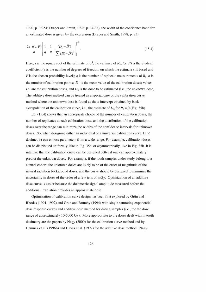
126

1990, p. 38-54; Draper and Smith, 1998, p. 34-38), the width of the confidence band for

an estimated dose is given by the expression (Draper and Smith, 1998, p. 83):

1/2_

2

_2

( )2 ( , ) 1 1

( )

x

i

D Ds t P

a q nD D

′−⋅ ν + +

′ ′− ∑

. (15.4)

Here, s is the square root of the estimate of σ2, the variance of Rx; t(ν, P) is the Student

coefficient (ν is the number of degrees of freedom on which the estimate s is based and

P is the chosen probability level); q is the number of replicate measurements of Rx; n is

the number of calibration points; 'D is the mean value of the calibration doses; values

Di´ are the calibration doses, and Dx is the dose to be estimated (i.e., the unknown dose).

The additive dose method can be treated as a special case of the calibration curve

method where the unknown dose is found as the x-intercept obtained by back-

extrapolation of the calibration curve, i.e., the estimate of Dx for Rx = 0 (Fig. 35b).

Eq. (15.4) shows that an appropriate choice of the number of calibration doses, the

number of replicates at each calibration dose, and the distribution of the calibration

doses over the range can minimize the widths of the confidence intervals for unknown

doses. So, when designing either an individual or a universal calibration curve, EPR

dosimetrist can choose parameters from a wide range. For example, calibration doses

can be distributed uniformly, like in Fig. 35a, or asymmetrically, like in Fig. 35b. It is

intuitive that the calibration curve can be designed better if one can approximately

predict the unknown doses. For example, if the tooth samples under study belong to a

control cohort, the unknown doses are likely to be of the order of magnitude of the

natural radiation background doses, and the curve should be designed to minimize the

uncertainty in doses of the order of a few tens of mGy. Optimization of an additive

dose curve is easier because the dosimetric signal amplitude measured before the

additional irradiation provides an approximate dose.

Optimization of calibration curve design has been first explored by Grün and

Rhodes (1991, 1992) and Grün and Brumby (1994) with single saturating exponential

dose response curves and additive dose method for dating samples (i.e., for the dose

range of approximately 10-5000 Gy). More appropriate to the doses dealt with in tooth

dosimetry are the papers by Nagy (2000) for the calibration curve method and by

Chumak et al. (1996b) and Hayes et al. (1997) for the additive dose method. Nagy

127

(2000) showed that the best distribution of calibration doses is the one that has the

central part close to the value of the unknown dose. The additive dose method presents

then the worst situation, because the back-extrapolated dose is external to the range of

the calibration points. However the dose distribution can be optimized to reduce the

uncertainty in the back-extrapolated dose. Hayes et al. (1997) and Nagy (2000)

demonstrated that the so-called “end point design”, i.e., the distribution with all the

calibration in the ends of the calibration range (similar to the example of Figure 35.b) is

best, whereas the uniform dose distribution gives the highest uncertainty in the back-

extrapolated dose. Hayes et al. (1997) developed a mathematical approach to derive the

optimal spacing between calibration doses based on the relative value of an initial

estimate of the unknown dose and the maximum dose to give to the sample. Chumak et

al. (1996b) evaluated the best number and values of additive doses in the case of

equally-spaced additive doses. Results of these studies show that it is worthwhile to

perform this kind of analysis before creating a calibration curve.

Best calibration curve fits are usually determined on the hypothesis that the

calibration doses are known exactly, which means that their uncertainties are negligible

in comparison with the uncertainties in the EPR signal measurements (see Chapter 17

and Appendix III dealing with uncertainties). Irradiation in a laboratory can be

performed with radioactive isotopes (typically 60Co, 137Cs, or 90Sr) or with an equipment

generating radiation, such as accelerators or x-ray machines. The source may have been

designed for experiments that do not require highly accurate dosimetry and, therefore,

the uncertainty in the doses given to tooth enamel with it may be significant. The

uncertainty of dose calibrations with primary and secondary standard sources is

approximately ±1% (1σ) or lower.

Calibration laboratories usually provide calibrations in terms of air kerma or,

increasingly, dose to water. In order to determine doses to tooth enamel, one needs a

conversion factor, which, in the simplest case, is the ratio of the spectrum-averaged

mass energy-absorption coefficient of enamel to that of air or water (Eq. (II.3) in

Appendix II). Since a standard composition for enamel has not yet been defined, the

energy absorption coefficient of enamel can be replaced with that of hydroxyapatite,

bone or, more frequently, of a compound of elements composing enamel. Different

elemental compositions were used (e. g., Wieser et. al, 2002; Takahashi et al., 2003).

128

The material of the sample holder should provide conditions as close to charged particle

equilibrium (CPE) in the sample as possible (see also Appendix II). Plastics whose

densities and compositions are similar to those of biological tissues (muscle, bone) or to

water are typically used. A list of suitable materials and their radiation properties can

be found in an ICRU Report (1989). The material most commonly used as a substitute

for soft tissues is polymethylmetacrylate (PMMA), also known as Plexiglas and Lucite.

However, PMMA becomes less equivalent to tooth enamel when the photon energy

decreases, and, at energies below 200 keV, the presence of elements like phosphorus

and calcium render the mass energy-absorption coefficient of enamel significantly

higher than that of PMMA. Based on Monte Carlo calculations, Ivannikov et al. (2004a)

concluded that, for the 60Co energy, the dose to enamel is 1.07 higher than the dose to

water if the sample is modelled with a 0.2-0.5-mm thick layer of uniform tooth enamel

located between 4-mm PMMA plates for CPE. No effect of sample thickness was found

when PMMA was replaced with aluminium in the model. A bone-equivalent plastic

B100 (ICRU, 1989) is commercially available, but there are no reports of its use in

tooth dosimetry. Furthermore, the sample was modelled as a uniform block of enamel

in the above calculations, whereas tooth enamel is usually irradiated in powder form, i.

e., the composition of the sample holder is an inhomogeneous mixture of enamel and

air. In this case, edge effects may take place at the grain surface when secondary

electrons escape from the enamel grains, thus failing to contribute to the dose in enamel

(Ivannikov et al., 2004a).

15.4 Parameters affecting the sensitivity of tooth enamel to radiation

Retrospective dosimetry with tooth enamel relies on the hypothesis that the radiation

sensitivity of the enamel at the time of dose reconstruction is similar to its sensitivity

during the in vivo dose accumulation. This is the reason why much attention has been

paid to the effect of sample preparation on its radiation sensitivity. Preparation

treatments can induce changes in the tooth enamel structure that may alter its sensitivity

to radiation (Section 10.9).

In order to preserve the natural radiation sensitivity, it is probably safer to treat the

sample as lightly as possible. For this reason, some authors prefer to use a mild

mechanical procedure without any chemical treatments (Ivannikov et al., 2002b).

129

Imperfect and nonuniform elimination of dentine from different samples can result

in significant nonuniformity of the radiation sensitivity. That was suggested by Wieser

et al. (2001), who found a 10% variability of the radiation sensitivity among samples

prepared with slightly different versions of the same sample preparation protocol. It is

therefore important that the same procedures be rigorously applied to all samples.

It is widely accepted that the radiation sensitivity of tooth enamel decreases with

decreasing size of grains in a powdered sample. Indeed, Sholom et al. (1998a)

irradiated enamel powder samples of grain sizes ranging from less than 75 µm (the

exact dimensions were not reported) to 800 µm. The radiation sensitivity was

independent of grain size from 800 µm down to 150 µm, below which a small decrease

of the radiation sensitivity was detected. A maximum decrease of 8% was observed at

grain sizes below 75 µm. This was explained by an increase of the surface-to-volume

ratio resulting in a smaller concentration of stable bulk paramagnetic centers. As a

consequence, it is now accepted not to use grain sizes smaller than 150 µm. However,

the situation may be more complex than presented by Sholom et al. (1998a). Iwasaki et

al. (1993) reported a 10% higher radiation response for grains smaller than 75 µm in

samples irradiated before grinding, which was attributed to an underlying distortion of

the baseline between 0 and 500 mT. Finally, the possible effect of absence of secondary

electron equilibrium during irradiation should not be overlooked (see above and

Ivannikov et al., 2004a).

Another factor affecting the radiation sensitivity is the stability of the paramagnetic

centers in time after irradiation. Sholom et al. (1998a) reported an increase of the

radiation sensitivity up to 15% in about a month after irradiation with subsequent

stabilization. This increase was attributed to transient signals of an unknown origin and

could be only partially explained by the unstable CO33- radical, which decays almost

completely within one day after irradiation (Section 8.10). Skinner et al. (2000)

reported substantial variations of the signal amplitude of fossil samples in the first 18

months after irradiation. Such a low stability was explained by formation of radicals at

the crystal surface, which could easily react with oxygen and water vapor. The results

by Skinner et al. (2000) could not be confirmed by Grün and Ward (2002).

Nonetheless, based on the results reported by Sholom et al. (1998a), it is now widely

recommended to perform measurements at least 15 days after the irradiation. Sholom et

130

al. (1998a) measured peak-to-peak amplitudes of the dosimetric signal; so, contributions

from the dosimetric and other signals to the spectrum had not been separated. Repetition

of these experiments with spectrum decomposition and isolation of the dosimetric signal

could provide new information.

The calibration curve method is based on the assumption that the intersample

differences in sensitivity are negligible. In principle, this assumption needs to be

proven, because tooth enamel, like any other biological tissue, shows some variability.

The radiation response may therefore depend on several factors that are either intrinsic

to the specific tooth, such as its age and carbonate content, or related to the donor (e. g.,

gender or ethnical group). Slight differences in carbonate content, crystal dimensions or

other chemical and physical properties of tooth enamel may induce variations in the

radiation sensitivity not only among tooth samples of different individuals, but also

among enamel samples from the same person. Iwasaki et al. (1995) reported that

sensitivities of enamel from different persons varied by less than 10%, which was

comparable with the variation in the sensitivity of teeth of the same individual.

Ivannikov et al. (2000) found 7% and 14% variations in sensitivities of the front teeth

and molars, respectively (in groups of approximately 25 teeth). Wieser et al. (2001)

reported a maximum variability in sensitivity of 10%, but, interestingly, could not find

any correlation between the radiation sensitivity and the donor's age, gender, residence

location (Germany or Egypt) or tooth position (the 4th and 8th positions were compared).

This degree of intersample variation has been found acceptable for justifying use of a

universal calibration curve. However, El-Faramawy and Rühm (2007) showed recently

that the radiation sensitivity increases with the tooth age after eruption. The authors

attributed this result to a continuing odontogenesis in the first years after the tooth

eruption. Unfortunately, the number of teeth in this latter work was small, and the

statistical significance of the results was, therefore, low, as the authors admitted. Their

findings cannot be accepted as definitive at this time, but, if confirmed, they will

probably impose a constraint on using young teeth in creating calibration curves.

It is well known that caries is associated with a high carbonate-to-phosphate ratio

(Section 3.5). Brik et al. (1996) reported that diseased teeth contain (5 – 15)% more

carbonate than sound ones. This may result in higher sensitivity of carious teeth (or, at

least, carious fractions of teeth) to radiation. Indeed, according to Brik et al. (1996), the

131

radiation sensitivity of carious teeth at doses above 10 Gy is approximately (20-50)%

higher than the sensitivity of sound teeth. This difference has not been observed at

lower doses. Sholom et al. (2000) studied the differences in the sensitivity between

carious and sound fractions of the same teeth at the 10 Gy dose level and found

variations below 10%.

It has been hypothesized that carious teeth have not only higher carbonate content,

but also poorer ordering of microcrystals (Cevc et al., 1976; Cevc et al., 1980; Brik et

al., 1996; Section 3.5). However, the results by Cevc et al. (1976, 1980) could not be

(fully) reproduced by Martens et al. (1986), who found no difference in ordering

between sound teeth and sound parts of teeth with caries. An explanation for these

findings may be that the same tooth can have parts that are really healthy (and, thus,

with “normal” carbonate content and crystal ordering) and parts that only look sound,

but are, in fact, likely to become carious shortly (and, thus, have lower crystal ordering

and higher carbonate content). Brik et al. (1996) noted that the radiation sensitivity

depends, in a complex way, on the number of precursor centers and on the trap depth

(i.e., the activation energy). The difference in the properties of the crystallites may give

rise to different activation energies of the traps, which may be the reason why the excess

of carbonate in carious teeth does not result in the expected increased sensitivity to

radiation. The effect of caries probably needs to be investigated further, possibly with

tooth enamel samples that have undergone artificially induced decay in vitro (Bhat,

2005).

15.5 Advantages and disadvantages of “the calibration curve“ and “the

additive dose” methods

With the factors affecting the radiation sensitivity discussed, the pros and cons of

the calibration curve and the additive dose methods can be explained better.

The calibration curve method offers the advantage that a sample with an unknown

dose does not have to be irradiated additionally, which leaves it unchanged for possible

reassessment of the dose in the future. Its obvious disadvantage is the need for a

collection of a large number of samples for constructing a statistically valid calibration

132

curve. However, once the calibration curve is constructed, an unknown dose can be

determined very rapidly.

A limitation of the additive dose method is that it takes a long time to perform

several additional irradiations and store the sample between each irradiation and the

subsequent measurement. The main advantage of the additive dose technique over the

calibration curve method is that the specific radiation sensitivity of the enamel sample is

used in the dose reconstruction, as opposed to the average sensitivity obtained from

other teeth. To counter this limitation of the calibration curve method, Hayes et al.

(1997) proposed to measure the individual sensitivity of the tooth under study by

irradiating a small aliquot (some 10 mg) to a high dose, so that the universal calibration

curve can be corrected for the individual sensitivity of the particular tooth. With this

approach, the time-consuming procedure of the additive dose method is avoided, and

the largest part of the tooth is left unirradiated.

In the 3rd international intercomparison (Wieser et al., 2005), the calibration curve

and the additive dose methods were used by seven and five laboratories, respectively.

Because many laboratories sought to provide the best achievable results in this

international exercise, they used the additive dose method, which is probably superior.

However, we are aware of only one group (Chumak et al., 1999) that used the additive

dose method in measurements of tooth samples of large groups of population; other

groups prefer to use universal calibration curves (Nakamura et al., 1998a; Ivannikov et

al., 2004a; Wieser et al., 2006b; Degteva et al., 2005, to mention a few).

16. The energy dependence of the EPR response of tooth

enamel

16.1 Theoretical background

The “energy dependence of the EPR response of tooth enamel” is an issue that is

often misunderstood, and, in order to clarify the core of the problem, we will start with

the basic theory. We refer the reader to Appendix II for definitions of the main

physical dosimetric quantities.

133

It is clear even from Lambert’s law originally developed for visible light (see

Appendix II) that, when a radiation beam enters a sample, only a fraction of the

travelling particles will interact with the atoms and deposit energy. This fraction of

particles can be very small (as is the case when the particles are high energy photons)

and depends on (i) radiation type and energy and (ii) the elemental composition of the

sample (see Appendix II). As a consequence, if two identical tooth enamel samples are

placed in two particle beams of different energy, the number of interacting particles,

and thus the absorbed dose, will be different even if the energy fluences are the same.

Similarly, two different materials placed in the same radiation field will receive

different doses under the same irradiation conditions.

The energy dependence of the absorbed dose, as described above, can be quite

easily predicted because the theory that makes it possible to calculate the fraction of

interacting particles is well developed. The problem essentially boils down to the

calculation of the mass energy-absorption coefficient defined in Appendix II. This first

contribution to the energy dependence of the EPR response on the energy, i.e., the

energy dependence of the absorbed dose on the energy (further referred to as “Factor

1”), will be explained further in the following paragraphs.

However, there is also another contribution to the energy dependence of the EPR

response. Even when the radiation doses (absorbed energies) in identical samples are

the same, but provided by radiation of different types, the effect, or damage, to the

sample may still be very different. As already discussed in Chapter 11, it can be

imagined that some radiation types produce more paramagnetic centers than others. To

further clarify this, consider, again, an example from another field, namely, silver halide

photography.

It is well known that photographs can be either under- or overexposed and that

this is related to illumination time and light intensity. These phenomena illustrate

failures of the so-called reciprocity law, namely, low-intensity reciprocity failure (LIRF)

and high-intensity reciprocity failure (HIRF), respectively. According to the reciprocity

law, the effect of light on a silver halide microcrystal in an emulsion should be

independent of illumination time and intensity, provided that their product (total

absorbed light energy) remains constant. It is not too difficult to explain LIRF and

HIRF if one recalls the general mechanism of silver halide photography. A single

134

microcrystal becomes developable (black) if it contains a so-called latent image, i.e., a

cluster of at least four silver atoms. These clusters are formed by combination of

photogenerated electrons and very mobile interstitial silver ions. LIRF can then be

explained essentially by the instability of the silver atom, i. e., the first intermediate

towards the Ag4 cluster. The electrons do not arrive sufficiently fast (intensity too low)

to let it grow to a stable (but undevelopable) Ag2-cluster, and the atom decays again (the

electron gets lost). No matter how high the total energy absorbed by such a

microcrystal is, a developable cluster will not be formed. On the other hand, when the

intensity is too high (HIRF), too many stable Ag2 clusters will form, which will lead to

an unnecessary large (and thus inefficient) number of latent image clusters (Tani, 1995).

Returning to EPR dosimetry, one could replace the ability to create a latent

image with the ability to produce a dosimetric paramagnetic center (CO2-). This latter

contribution to the energy dependence of the EPR response (further referred to as

“Factor 2”) is, obviously, very hard to calculate. Several authors have attempted to

answer the question whether the EPR response of a tooth enamel sample irradiated to

the same absorbed dose would be the same regardless of the radiation type and energy.

Although it is rather intuitive and obvious theoretically, experiments to prove this

statement and to quantify the effect are complicated by a number of factors, and

published results may seem confusing or contradictory (see below).

The energy dependence of a dosimeter response is determined by the

dependence of its radiation sensitivity (i.e., the dosimeter reading, R, per unit dose, D)

upon the radiation energy (Attix, 1986, p. 283). However, the term ‘energy dependence’

is not defined unambiguously in the scientific literature. In some papers, it means the

energy dependence of a dosimeter reading per unit dose to the dosimeter material (only

the Factor 2 described above is involved). In other papers, it means the energy

dependence of dosimeter reading per unit dose to a reference material (typically water)

under the same conditions, which effectively comprises both the factors described

above. At first sight, it looks like a simple arbitrary change of the medium, but, in

reality, the difference between the two definitions goes far beyond.

The former definition reflects only the energy dependence of the intrinsic

detector efficiency, i.e., the dependence of the dosimeter response to the same dose

absorbed by the same dosimeter material on type and energy of the radiation that

135

provided this dose. In fact, if a unit absorbed energy produces the same measurable

effect at every photon or particle energy, then the detector response per unit dose is

independent of energy. As Attix (1986, p. 288) pointed out, the study of the energy

dependence of the intrinsic detector efficiency is the most interesting from a dosimetric

viewpoint, since it cannot be predicted by interaction probability characteristics.

The latter definition of energy dependence reflects, by contrast, also the

difference between the energy dependences of the dose absorbed in the dosimeter and of

the dose absorbed in a reference material under the same conditions. In fact, radiation

fields are usually calibrated in terms of dose to water or in terms of air kerma (Appendix

II). It is then essential to convert the reference dose into the dose to the dosimeter

material. This factor in the “energy dependence of EPR response” can be predicted by

calculating the interaction probabilities of the incident beam radiation with the

dosimeter atoms (or the mass energy-absorption coefficient).

The energy dependence of the detector response per unit dose to the dosimeter

material, Ddos, and to the reference medium, Dmed, can then be mathematically

expressed as

dos medR D D fε ε= = , (16.1)

where f is a factor that reflects the probabilities of the interaction of the radiation field

with the detector and reference medium materials (Factor 1), while ε is the intrinsic

detector efficiency (Factor 2). Both ε and f may depend on radiation energy.

The energy dependence of the intrinsic detector efficiency can be estimated

accurately only if the factor f is calculated with sufficient precision. For this reason, we

will briefly discuss the calculation of f, assuming for the moment ε to be energy-

independent.

Calculation of f (Factor 1 for the reference and dosimeter materials)

Conventionally, energy dependence of a dosimeter response is described using its

relative sensitivity, i.e., the dependence of radiation sensitivity upon radiation energy,

normalized to the sensitivity of the same dosimeter in a reference beam, usually 60Co

(assuming ε to be constant):

136

[ ][ ]

0 0

( )

( )

Emed E

E Emed

RfD

R fD

− −

= , (16.2)

where−

E is the radiation spectrum averaged energy (or the radiation energy if the

incident beam is monoenergetic); E0 is the reference beam energy (typically the 60Co

energy). Normalizations to air kerma or exposure instead of dose to a medium or to

reference beams other than 60Co are sometimes used.

As an example, let us consider a tooth enamel sample irradiated with a photon

beam under charged particle equilibrium conditions (CPE, see, e.g., Attix, 1986) and

assume negligible beam attenuation in the sample volume (linearization, see above)

and energy-independent intrinsic detector efficiency ε. In this case, the general

expression for the relative sensitivity of Eq. (16.2) becomes

[ ][ ]

0

0

0

( )( )

( )( )

( )( )

( )( )

− − −

−

≅

enenamel

enamelen

medmedE E E

enenamelEenamel

med Een

medE

E

D Ef D

Ef D

DE

µρ

µρ

µρ

µρ

, (16.3)

where µen is the mass energy-absorption coefficient described in Appendix II. It

relates absorbed dose to energy fluence ψ and depends on both the properties of the

material and the radiation energy. With known energy spectrum and elemental

compositions of the dosimeter and reference material, the term on the right of Eq.

(16.3) can be directly calculated by the tabulated values of mass energy-absorption

coefficients (it has become a common practice to use Monte Carlo for this calculation,

although it is not necessary). In the case of particles other than photons, equations

similar to Eq. (16.3) can be written using other quantities instead of the mass energy-

absorption coefficient (Attix, 1986).

The energy dependence of the ratio in Eq. (16.3) for photons has a characteristic

shape reflecting the energy dependence of the cross sections for the various

mechanisms of interaction of photons with matter. Of many interactions theoretically

possible, only photoelectric effect, Compton scattering and pair production are of any

137

significance for photons (see Appendix II). The probability of each type of interaction

depends in its own, specific way on photon energy and average (effective) atomic

number. For low-Z materials and photon energies below 0.5 MeV, the dependence of

the absorption ability on photon energy is determined by the competition between

Compton scattering and photoelectric effect, and, at a few tens of keV, the latter

dominates the former (see, for instance, Attix, 1986, pp. 124-125). For all materials of

interest in radiation protection (air, water, muscle, bone), Compton scattering becomes

significant even at photon energies below 100 keV. If the effective atomic number of

the dosimeter is higher than that of the reference material, the dependence of the

relative sensitivity on energy follows a bell shape with a maximum at an energy below

100 keV. The response per unit dose will be then higher at low energies than at 60Co.

By contrast, if the effective atomic number of the dosimeter is lower than the effective

atomic number of the reference material, its relative sensitivity will monotonously

decrease with decreasing energies. It is then straightforward that the curve is reduced

to a constant if the reference medium is the same as the dosimeter medium.

As already mentioned above, Eq. (16.3) is obtained under the ideal assumptions

of CPE, negligible attenuation of the incident beam in the dosimeter volume and

energy-independent intrinsic detector efficiency, otherwise more complex functions

must be used to calculate the theoretical curve (details can be found in any book of

radiation interactions with matter; see, for instance Attix, pp. 283-288).

The real curve can deviate from the theoretical curve described by Eq. (16.3) if

the dosimeter elemental composition used in the calculation is incorrect. Small

differences between the real and the assumed elemental composition can lead to very

different mass energy-absorption coefficient, especially at low energies. For a given

material, ( )

enEµ

ρ is calculated by the Bragg rule as the sum of the mass energy-

absorption coefficients of the elements composing the material weighed by elemental

mass fractions (Attix, 1986, p. 156). Since the exact composition of tooth enamel is not

known, the ( )

enEµ

ρ must be calculated for hydroxyapatite or bone using Bragg’s rule.

Schauer et al. (1993) have clearly demonstrated that errors in assumptions on material

composition can lead to “apparent” energy dependence of the dose response.

138

Imperfect knowledge of the radiation energy spectrum is another source of

uncertainty in calculations of the mass energy-absorption coefficients. Strictly speaking,

the energy spectrum of x-ray beams should be used in the calculations. In many cases,

however, it is unknown, and the equivalent monoenergetic photon energy is used

instead. Schauer et al. (1993) have shown that, in some cases, the use of this quantity

produced errors in the f factor of 20% or more. Sometimes, alternative quantities are

used to describe an x-ray beam, namely, the nominal applied voltage, spectrum

averaged energy, full range of energy or its ISO standard code (ISO, 1996). These

characteristics are likely to produce even less reliable predictions of ( )

enEµ

ρ .

Moreover, if the tooth was irradiated in vivo (i.e., in the mouth) or in phantoms,

modification of the energy spectrum in the tooth position should be accounted for in the

calculation of ( )

enEµ

ρ .

Finally, to be of interest for dose reconstruction studies, the tooth enamel dose

response must be transformed into other meaningful radiation protection quantities,

such as dose to organs. This is achieved through conversion factors calculated by

simulation of interaction of radiation with anthropomorphic model phantoms. It is

usually performed through an intermediate transformation of the dose in enamel to air

kerma followed by a further transformation of the latter to dose to the organs of

interest.

Literature results will be discussed in the following sections, but it was not always

possible/easy to eliminate the confusion explained above.

16.2 Energy dependence of the EPR response in photon fields

The energy of photons to which tooth enamel of an individual can, in principle, be

exposed ranges from a few tens of kiloelectronvolts to several megaelectronvolts. The

energy spectrum of the natural gamma radiation extends up to approximately 2.6 MeV,

with the spectrum-averaged energy around 700-800 keV (UNSCEAR, 2000b). Medical

treatments are also a significant source of photon exposure, at least in the countries with

the highest level of health care. It has been estimated that 92% of the population of such

nations undergoes a diagnostic x-ray examination every year (UNSCEAR 2000a). The

139

photon beam energy in this case is usually of the order of tens of kiloelectronvolts.

Other external photon exposure can occur on workplaces and on accidentally

contaminated locations.

Several authors have experimentally evaluated the dependence of the EPR response

of tooth enamel per unit dose as a function of photon energy, mainly at energies below

1 MeV (Ikeya et al., 1986; Aldrich and Pass, 1988; Schauer et al., 1994; de Oliveira et

al., 1999; Wieser et al., 2002; Ivannikov et al., 2004b). Table 16.1 shows a panorama

of the results reported in the literature. Since some figures were derived from graphs in

the papers and are, therefore, only approximate and, besides, quite a few papers did not

include an analysis of the uncertainties, the values listed in this table have to be taken

only as indicative of a trend. The dose response of tooth enamel per unit dose to

enamel-like tissues (bone or hydroxyapatite), normalised to the response at the 60Co

energy, is unity, as expected from the theory, except at the very low energies. As

explained in the previous section, this result means that the tooth enamel intrinsic

efficiency (ε) is energy-independent. The radiation response in enamel per dose to air,

normalized to the response at the 60Co energy, shows the highest values at applied

voltages between 50 and 100 kVp or at a spectrum-averaged energy close to 50 keV.

Ivannikov et al. (2004b) evaluated, both experimentally and theoretically, the

energy dependence of the EPR response of tooth enamel in x-ray beams with average

energies between 0.0129 and 0.208 MeV. In the calculations, the authors took into

account the x-ray energy spectra and beam attenuation in the material. They evaluated

the energy dependence of the ratio of the experimental (EPR) to the calculated dose

response of enamel and found a deviation of this ratio from unity at energies below 30

keV. According to the authors, the decrease of the ratio at the low photon energies was

likely due to an incomplete description of the irradiation geometry and enamel sample

shape in the calculations rather than due to the intrinsic energy dependence. In

particular, a powder sample was used in the experiment, whereas the calculations were

performed for a plate. Therefore, secondary electrons escaping from the grains did not

contribute to the experimentally measured absorbed dose, but their contributions were

included in the results of the calculations.

Role of surrounding body parts

140

The energy dependence of the radiation response of tooth enamel irradiated free-in-air

has a speculative, but not a practical use. In fact, in an exposure in vivo, the intensity

and the energy spectrum of the radiation photons incident on the tooth are modified by

traversed cheeks and bones. Therefore, the tooth response depends on the position of

the tooth in the mouth and on the direction of the radiation field with respect to the

head. The radiation responses of teeth placed in a phantom simulating a head are more

interesting because they simulate the real situation, although even a phantom is a rough

approximation of the human head. Takahashi et al. (2001, 2002, 2003) and Ulanovsky

et al. (2005) have used Monte Carlo simulations to calculate the photon dose

conversion factors for tooth materials in an anthropomorphic phantom in the 0.01-10

MeV energy range for several geometries of exposure (antero-posterior, isotropic, top-

ground, etc.). Despite some differences in the calculation (use of a voxel or

mathematical phantom, detail of tooth geometry, enamel/dentine distinction, separate

buccal/lingual dose calculation), the results of the two studies lead to similar

conclusions, as demonstrated by Ulanovsky et al. The dose conversion factors depend

on energy nonlinearly at photon energies below approximately 300 keV, with a

maximum between 50 and 90 keV (an example is shown in Fig. 36 for an antero-

posterior irradiation). At the maximum, the dose in enamel can overestimate the air

kerma as much as by a factor of 10. They found that, in certain irradiation geometries,

the energy dependence of the tooth response depends significantly on the location of

the tooth in the mouth. Both calculations have been verified experimentally with

parallel measurements of doses to tooth enamel (by EPR) and to TLD dosimeters

(Wieser et al., 2002; Takahashi et al., 2003).

The conversion factor of the dose to enamel to the dose to air in the radiation field

of the natural background has been reported only in the paper by Ivannikov et al.

(2000), who calculated the correction factors for energy dependence of enamel

sensitivity for real radiation fields in regions contaminated by the Chernobyl accident.

According to their estimate, the dose to air after exposure to the natural radiation

background radiation can be determined by correcting the tooth enamel dose response

to 60Co by a factor of approximately 0.8.

141

Medical doses

Medical exposures are confined to the body region of interest and rarely involve the

whole body. An examination of the chest has been demonstrated to give a maximal

dose to tooth of only about 0.2 mGy per exposure (Sholom et al., 1998b). Therefore,

only dental examinations are of interest for tooth enamel dosimetry. Using a head-like

phantom, Aragno et al. (2000) have experimentally found that the dose to enamel from

an examination performed with modern x-ray endoral equipment is 2 mGy per

exposure. El-Faramawy (2005b) measured the dose to enamel of 17 teeth from donors

who had received a known number of dental diagnostic x-ray exposures and found an

absorbed dose of 4.0±2.9 mGy per x-ray exposure. However, with different equipment,

doses per single exposure may be as high as 60-70 mGy (Sholom et al., 1997); so, in

principle, the possibility of past examinations should not be overlooked because they

can be a distort results of dose assessment. The dose from an orthopantomographic

examination with modern equipment has been approximately estimated as 0.2 mGy

(Aragno et al., 2000).

Aldrich and Pass (1986) have proposed a method to separate the dose due to the

natural background from the dose due to x-ray examinations using the attenuation

coefficient of x-rays in tooth. That paper inspired works by Hayes et al. (2000b, 2003)

and Sholom et al. (1997), who also emphasized the role of the absorption of the

scattered radiation in the difference between the doses to the labial/buccal and lingual

sides of teeth. The x-ray beam attenuation in the tooth was investigated by some

authors, who experimentally evaluated the radiation response of tooth enamel in the

buccal and lingual half parts of a tooth separately (Aldrich and Pass, 1988; Wieser et

al., 2002). Aldrich and Pass have found approximately 80% attenuation by a tooth at

50 kVp and approximately 50% attenuation at 100 kVp. Wieser et al. (2002) have

reported attenuation between 7% and 35% for teeth in different positions inside a

phantom simulating the head, which was irradiated with a 80-kVp beam. Although the

results by Wieser et al. seem to show weaker attenuation, it is hard to compare the

results of the two studies unambiguously because, in one of them (Aldrich and Pass,

1988), the mass energy absorption coefficients were evaluated at the nominal voltage

and in pure enamel, while, in the other, the real x-ray energy spectrum was integrated

and the calculations were performed for dentine and enamel separately (Wieser et al.,

142

2002). Schauer et al. (1994) have observed a trend of decreasing EPR signal intensity

in bone with increasing sample thickness in the range 0.5 - 2 mm at an average energy

of 34 keV (in an ISO M60 x-ray calibration beam). The decrease was estimated to be

about 17 % in 1 mm and might be due to attenuation of the primary beam in the

sample.

By contrast, doses to teeth from radiation therapy treatments are very high (a few

Gy or even higher), especially if the tumor is in the head-and-neck region (Pass et al.,

1998). Therefore, tooth samples of treated patients can be easily identified, but they are

usually excluded from the dose reconstruction in epidemiological studies.

16.3 EPR response of tooth enamel to doses received in neutron fields

Exposure to neutrons may occur in such events as nuclear plant accidents, medical

radiation incidents, in aviation and outer space travel (IARC, 2000), and the neutron

energy spectrum can vary widely, ranging from 1 keV – 1 MeV in a reactor to 10 GeV

for secondary neutrons in space. If tooth enamel dosimetry is to be used in such cases,

the impact of neutron contribution to the total enamel dose should be known.

Interpretation of the energy dependence of tooth enamel response to neutron

fields is complicated by several factors. One of them is the unavoidable presence of

gamma photons in the radiation field. The cumulated dose in tooth enamel, DE, in a

mixed field can be expressed with the conventional formula (ICRU, 1977; CEC, 1985)

E nD kD hDγ= + , (16.4)

where k is the relative radiation sensitivity to neutrons and h is the relative radiation

sensitivity to the photon component of the mixed field, both normalized to the 60Co

sensitivity; Dn and Dγ are the neutron and photon absorbed doses in tissue in the mixed

field. The value k can be obtained from Eq. (16.4) as

E

n

D hDk

D

γ−= , (16.5)

where DE is evaluated by EPR and separate contributions Dγ and Dn must be evaluated

with independent methods.

A further problem is that the majority of neutron beams that are used to test the

EPR response of tooth enamel in the laboratory are not monoenergetic. In most studies

143

of the tooth enamel response to neutrons, tooth samples were irradiated in reactors

(Zdravkova et al., 2003a ; Trompier et al., 2004) or in radiation therapy beams

(Zdravkova et al., 2002a), all of which are characterized by wide energy spectra. Two

groups investigated the radiation response of tooth enamel in neutron generators,

which produce quasi monoenergetic particles (Fattibene et al., 2003; Khan et al.,

2003c; Fattibene et al., 2004a; Fattibene et al., 2004b).

Neutrons do not release energy in a continuous process because they undergo

several kinds of interactions with the matter, some of which have energy thresholds.

Therefore, the energy dependence of the kerma factor (Fn, a quantity similar to the

mass energy-absorption coefficient used for photons) is a discontinuous function.

Moreover the energy delivered to matter by neutrons may be uncorrelated with the

EPR signal. For example, if the neutron travelling in tooth enamel hits an impurity

nucleus producing a (n, α) reaction, the emitted α particle will release its energy within

a few microns. If this "hot spot" is far from carbonate molecules, there will be no EPR

response.Even a very small percentage of impurities with high cross sections to

neutrons can unpredictably change the response of the dosimeter. It is because of this

kind of mechanisms that tooth enamel response per unit radiation dose in neutron fields

might strongly depend on neutron energy.

Finally, when irradiated in vivo, tooth enamel is surrounded by tissues with higher

hydrogen contents, such as dentine and, especially, the muscle tissue of the head. The

interaction between a proton (hydrogen nucleus) and a neutron has a high cross section

due to their similar masses. As Tikunov et al. (2005) have shown, the secondary

protons produced by the elastic scattering of the fast neutrons on hydrogen nuclei

contribute significantly to dose in enamel. For this reason, the majority of the

published studies are focused on the irradiation of whole tooth samples in phantoms

that simulate human head.

The first work about neutron response of tooth enamel was published in 1997

(Bochvar et al., 1997). The authors reported a theoretical estimate of the neutron

sensitivity of hydroxyapatite to fast neutrons of 1 keV-1 MeV resulting in a value

about 33 times lower than that of gamma-rays. Although the paper had its limits

because the calculation was performed on hydroxyapatite (instead of enamel) and in air

(i.e., ignoring the effect of the surrounding tissues and dentine on the energy

144

spectrum), it was the only existing publication (except of a paper by Tatsumi (1986) in

Japanese reporting that tooth enamel is not effective in detecting 14 MeV neutron

exposure). Based on the conclusion of this paper, the contribution of neutrons to the

total absorbed dose in enamel has been considered negligible for years.

The role of the tooth enamel response to neutrons was reconsidered more recently

because of its potential or actual relevance to dose reconstruction studies involving

neutrons (Nakamura et al., 1998; Romanov et al., 2002; Shiraishi et al., 2002). The

need for studying the neutron sensitivity of tooth enamel was also pointed out by ICRU

(2002). Between 2002 and 2004, the scientific literature has seen a boost of papers

about the subject (Zdravkova et al., 2002a; Fattibene et al., 2003; Khan et al., 2003c;

Zdravkova et al., 2003a; Fattibene et al., 2004a; Fattibene et al., 2004b; Trompier et

al., 2004; Tikunov et al., 2005; Trompier et al., 2006). Table 15.2 presents a summary

of results of these studies. When the reference medium was tissue, the neutron-to-60Co

(also indicated as n/γ) relative sensitivity was in the 0.03-0.15 range, and, in two

studies, it was even found undetectable. According to Fattibene et al. (2004b) the n/γ

relative sensitivity is approximately 0.2 at 2.8 MeV and 0.4 at 14 MeV when the

reference medium is air. The n/γ relative sensitivity was found to be 0.33±0.08 at 2.8

MeV and 0.47± 0.09 at 14 MeV when the tooth enamel EPR response was measured

per unit dose in enamel (Fattibene et al., 2003, 2004a). Like in the case of photons, the

deviation of the relative sensitivity from unity when the reference medium is tooth

enamel has two possible explanations: a) incorrect assumptions made for the tooth

enamel composition; b) a different intrinsic efficiency of the generation of radicals in

carbonate molecules of tooth enamel by neutrons.

An interesting application was presented by Zdravkova et al (2003a), who

measured the dose response of a whole tooth to neutrons using an L-band spectrometer

(see subsequent chapters of this review). Another paper relevant in this context, by

Trompier et al. (2006), describes use of the dentine-enamel system as a combined

dosimeter for measurements in mixed neutron and gamma fields. Despite the low

sensitivity of both the tissues to neutrons and various problems related to dosimetry

with dentine (Chapter 20), the proposed method could be useful in situations where

alternative methods to measure the gamma dose in a mixed field are not available.

145

16.4 EPR response of tooth enamel to doses from internal ββββ-emitters

Radiation sources can be located inside organs of a human body and irradiate teeth

from there. Among the radionuclides that may be present in our bodies, isotopes of the

elements contained in teeth are especially important in this context. These are the

radioactive isotopes of the constituting elements (such as 45Ca and 32P) and of trace

elements, such as Pb, Ra and Sr, which substitute for Ca easily (Driessens and

Verbeeck, 1990). We will focus mostly on 90Sr (a β-emitter) because most of our

present knowledge about EPR dosimetry of tooth enamel following internal

contamination deals with it. This is due to the huge number of studies performed in the

framework of dose reconstructions for residents of the Techa River territories in the

Southern Urals (Chapter 19).

When traversing a bone-like material, β-particles lose their energy in a range of

the order of millimetres, i.e., much shorter than the range of high-energy photons or

neutrons. Accordingly, radiation damage to tooth enamel is made only when an emitter

is inside the tooth enamel itself or in the dentine (and, to a lesser extent, when a

radioactive isotope is in other adjoining tissues, such as maxillary and mandible bones).

Processes of incorporation of radioactive isotopes in teeth are generally similar to the

processes described in Chapter 3 for stable elements, but they are not the same for all

tissues of a tooth. Tooth enamel captures radionuclides mainly before the tooth

eruption, and concentrations of these radionuclides hardly change thereafter. Further

incorporation is mainly due to ion transport between the enamel surface and

surrounding fluids. However, Tikunov et al. (2006), using low background β−counting,

detected non-negligible 90Sr concentrations in teeth already formed completely by the

time of contamination, which suggests that post-eruption uptake of radioisotopes by

enamel should not be ignored. Loss of minerals from tooth enamel is attributed mainly

to ion diffusion and tooth surface reactions. Strontium elimination is likely to occur by

the same processes as those affecting calcium elimination, i.e., diffusion, surface

dissolution or demineralisation and mechanical attrition (Suga and Watabe, 1992 ;

Tolstykh et al., 2003).

A dependence of the radionuclide concentration in tooth enamel on the tooth

mineralization stage was clearly evidenced by doses measured in teeth of the Techa

146

river residents. Significantly higher doses, up to approximately 15 Gy, were found in

teeth that were forming at the time of the 90Sr release, whereas the doses were below 1

Gy in the teeth that had already been completed at that time (Tolstykh et al., 2000;

Romanyukha et al., 2001). Because of the differences in the development processes of

teeth in different buccal positions, incorporation of radioisotopes into teeth of different

types occurs at different ages. However, incorporation of radioactive elements in

dentine can take place during the whole life of the tooth because dentine grows

throughout this period, as described in Chapter 3. Because radiation emitters get

incorporated in dentine also after tooth eruption, combined measurements of doses to

dentine and enamel of the same tooth may provide information about the time of the

contamination.

Dose accumulation in tooth enamel is thus a dynamic process, depending on the

time elapsed since the start of the intake, the radionuclide concentration and the

effective (i.e., the combined physical and biological) half-life of the radionuclide. It can

be easily understood that, because of the variety of processes and dynamics governing

the emitter incorporation in teeth, the resulted radionuclide distribution in the tooth

volume is not uniform. The non-uniformity of the sources, combined with the short

particle range, is reflected in a non-uniformity of the energy deposition of β-particles,

and, thus, of the radiation-induced radical distribution in tooth enamel. These factors

make the volume-averaged dose provided by EPR measurements of little significance

for short-range particles. Tolstykh et al. (2000, 2003) argued against the suitability of

EPR dosimetry with 90Sr contaminated teeth, in particular because the estimate of the

tooth enamel dose should account for the time dependence of the 90Sr content and

distribution not only in enamel, but also, and especially, in dentine. They concluded that

EPR tooth enamel dosimetry should be limited to the assessment of the external dose

component.

Sometimes teeth can be subjected to both external and internal exposure, as is the

case, e.g., of the residents of the Techa riverside. As pointed out before, we are not able

yet to distinguish between EPR dosimetric signals generated by different types of

radiation. Therefore, either the internal or the external contribution to a dose in tooth

enamel has to be determined by an independent method. Shishkina et al. (2001a) have

proposed such a procedure for the case of internal 90Sr contribution. It consists of two

147

steps: first, the radionuclide concentration in dentine is measured using different

methods; then, the dose rate in enamel per unit concentration of 90Sr in dentine is

calculated by a program providing Monte Carlo simulations. The dose absorbed in

enamel is then calculated as a product of the number of radioactive disintegrations of

90Sr per gram of dentine (estimated in the first step) and the corresponding dose rate

coefficient (DRC, the dose rate in enamel per unit of activity) (calculated in the second

step).

Hayes et al. (2002) have proposed a simplified model for measuring the internal

exposure in enamel due to a bone-seeking radionuclide. The method is based on the

assumption that 90Sr incorporation occurs almost completely in the jaw bone and at the

pulp cavity surface. However, the kinetics of 90Sr incorporation in dentine makes this

model unfeasible for teeth, as pointed out by Anspaugh et al. (2003).

We will now consider in greater detail how the two-step method proposed by

Shishkina et al. (2001a) can be implemented practically.

a) Measurement of the radionuclide distribution in tooth enamel and dentine.

When the radioactivity level is sufficiently high, the volume-averaged 90Sr

concentration can be obtained by the traditional in vivo tooth β−counters and in vitro

radiochemical methods (Tolstykh et al., 2000); otherwise, it can be measured by a

low-background β−counting set, such as used by Tikunov et al. (2006). Distribution

of the β-emitting radionuclide concentration can be mapped with two methods: thin

TLD (Goksu et al., 2002) and photostimulable phosphor imaging plates

(Romanyukha et al., 2002b; Shishkina et al., 2002).

b) Calculation of the dose rate in enamel per unit concentration of 90Sr.

Dose distribution in tooth enamel due to emitters incorporated in dentine, jaw bone

and enamel itself has been calculated with mathematical models. Two groups have

independently developed a Monte Carlo model to calculate doses to enamel from

90Sr incorporated in dentine (Seltzer et al, 2001; Tolstykh et al. 2000), in jaw bone,

and tooth enamel itself (Tolstykh et al. 2000). They used different Monte Carlo

codes and made different assumptions of the 90Sr deposition in the tissue sources.

Seltzer and his coworkers modelled a tooth as a dentine cylinder inside a

conaxial enamel cylinder. The cylindrical shape is usually regarded as appropriate

148

for molars and premolars. They ignored root dentine and cementum, and considered

a uniform 90Sr distribution over the whole dentine volume.

The model proposed in the paper by Tolstykh et al. (2000) and its upgraded

versions (Shved and Shishkina, 2000; Shishkina et al., 2001a) was more

sophisticated. The tooth was modelled as a set of coaxial cylindrical layers, each of

its own composition, which described the various tissues of a tooth (root dentine,

cementum, alveolar bone, pulp, crown dentine, tooth enamel and the enamel of the

neighboring teeth). Additionally, they assumed a non-uniform 90Sr distribution found

by radiometric measurements. In contrast to the case of self-exposure, crown dentine

and lateral enamel appeared more important for the dose in the masticatory enamel,

while crown dentine and cranial bone adjacent to the root contributed significantly

mostly to the dose to the lateral enamel. When the source of irradiation was dentine,

the DRC was found to be of about 0.01-0.02 (nGy/s)/(Bq/g), whereas, when enamel

was the source, the DRC was approximately ten times higher.

Both Seltzer et al. (2001) and Shved and Shishkina (2000) calculated the DRC

as a function of tooth dimensions, and significant differences (up to 60%) in the DRC

were found between small and large teeth. The agreement between the calculated

and the EPR-measured tooth enamel dose was better when a non-uniform 90Sr

concentration in dentine was assumed (Shishkina et al., 2001a). However, it is not

clear yet whether a larger number of coaxial layers in the tooth model (Shishkina et

al., 2001a) improve dose estimates.

The final issue to point out is that the dose produced by internal emitters in teeth

does not directly reflect the intake in skeletal bones, although many radionuclides have

similar affinity for tooth enamel and bone. Long ago, Goldman et al. (1967, 1972), who

injected animals with radionuclides, found that 90Sr content of a bone decreases

significantly throughout the person's life because of bone remodelling, in contrast to the

stable 90Sr content of enamel. More recently, Tolstykh et al. (2000, 2003) found that

there is a complex correlation between radionuclide accumulation in teeth (both dentine

and enamel) and in bone, which brought them to a conclusion that a conversion of a

tooth dose to the bone dose requires complex models. They compared data obtained by

radiochemical measurements of extracted permanent posterior teeth, in vivo

measurements of surface β −activity of the anterior teeth, and whole-body (counter)

149

measurements of 90Sr in the skeleton. The study revealed a weak correlation between

90Sr concentration in skeleton and teeth in adults (around 0.43-0.47), but no such

correlation for children and adolescents. Ignatiev et al. (1999) used EPR to measure

doses to teeth and bones of a dog injected with 90Sr. Although this mode of radionuclide

administration was very different from a typical contamination during accidental

exposures, it is interesting that doses to dentine and some bones were found to be

correlated, whereas there was no apparent correlation between doses to tooth enamel

and bones.

16.5 EPR response of tooth enamel to ultraviolet radiation

The existence of a UV-induced signal in tooth enamel similar to that induced by

ionizing radiation was reported almost simultaneously by Romanyukha et al. (1996d)

and, more extensively, Liidja et al. (1996). When this signal is practically

undistinguishable from the dosimetric signal (and is probably the same), it results in an

overestimate of the dose. Liidja et al. (1996) investigated the dependence of the

dosimetric signal intensity on the UV wavelength and found that the concentration of

induced radicals per unit of UV flux density decreased with the wavelength and had a

sharp edge between 305 and 335 nm. They found that the maximal EPR response of

tooth enamel to UV radiation with a typical solar spectrum on a sunny day is equivalent

to 10 mGy/(h nm).

Several reports of the EPR response of enamel to radiation from artificial UV lamps

(Ivannikov et al., 1997; Sholom et al., 1998b; Nilsson et al. 2001; El Faramawy, 2005a;

Jiao et al., 2007) followed these early papers. The newer papers reported the nominal

energy of the UV radiation emitted by the lamps, but not the spectra. They confirmed

that an EPR signal similar to the dosimetric one appears after illumination at an

average wavelength 254 nm, but irradiation at 365 nm does not produce it. A

comparison of the intensities of the "dosimetric-like" signal reported in these papers is

not straightforward because of the differences in the powers of the UV sources and in

source-sample distances. Moreover, most of these studies were carried out with a very

limited number of samples (Sholom et al., 1998b; Nilsson et al. 2001; El Faramawy,

2005a).

150

More interesting are papers that, based on the results of Liidja et al., have directly

investigated the effect of solar light on tooth enamel (Ivannikov et al., 1997; Sholom et

al., 1998 ; Jiao et al., 2007). Very different values of the 60Co-equivalent dose in

enamel were found: 500 Gy/mo (Ivannikov et al., 1997), 200 mGy/day (Sholom et al.,

1998b) and 20 mGy/h (Jiao et al., 2007). The apparent contradiction is probably due to

the different exposure geometries and sample grain size, because UV light gets

completely absorbed in approximately 100-200 µm of tooth enamel (Ivannikov et al.,

1997; Sholom et al., 1998b; Fattibene et al., 1998).

The paper by Jiao et al. (2007) is based on an investigation of 11 samples exposed

to sun light for one year and is, in our opinion, most sound statistically. Assuming

roughly 30 min of direct sun exposure of teeth a day, the authors evaluated the mean

value of the UV-induced dose equivalent as approximately 500 mGy over 50 years of

tooth life. This value may be an overestimate because it is unlikely that a person

exposes his teeth to direct sunlight for 30 min every day. Moreover, dispersed light has

been shown not to produce an additional signal (Ivannikov et al., 1997). Nevertheless,

it is clear that the UV effect cannot be ignored in estimating radiation doses to teeth. As

a conclusion, although the Earth surface is reached by sunlight of a broad spectrum

with wavelengths above 280 nm, UV generation of radicals in tooth enamel is small,

but it does exist.

No convincing evidence is available that the signal induced by UV light is the same

as the signal induced by ionizing radiation. Therefore, the UV-induced signal is often

cautiously called "dosimetric-like". Jiao et al. (2007) have reported that the microwave

power dependences of the UV-induced signal and the dosimetric signal are similar. Brik

et al. (2000) have offered a hypothetical mechanism of formation of CO2- radicals (from

CO2) induced by UV light, which has already been described in Eqs. (9.1) and (9.2) of

this review. The reasoning underlying such model is that UV energy is not sufficient to

knock electrons out of the CO32- ions or out of the crystal lattice (in order to form CO2

-

radicals from CO32- ) . The UV-induced signal may be different from the signal induced

by gamma radiation; the two may be formed by different paths; and the picture may be

even more complex because the mechanism of formation may depend on the UV

wavelength.

151

In addition to the dosimetric-like signal, two other signals have been detected both

in UV- and sunlight-exposed samples, centered around g = 2.0110 and g = 2.0052

(Sholom et al., 1998b ; Jiao et al., 2007). These signals are stable in time, saturate with

irradiation time and are perhaps the same signals as observed by Nilsson et al. (2001).

However, characterization of these signals depends on the method chosen to isolate the

UV-induced signal from the dosimetric and native signals. El-Faramawy (2005a) fitted

the experimental spectrum of tooth enamel with a combination of four signals (two

CO2- and two native ones) and studied their dependences on the UV irradiation time.

This author has not found (or has not reported) any signals at g = 2.0110 or g = 2.0052.

Authors of all the mentioned papers agree that some EPR signals from tooth enamel

irradiated with UV and gamma rays, once optimally characterized, could serve as

indicators of UV exposure.

Regardless of the origin of the UV-induced "dosimetric-like" signal, it is clear that,

when present, it results in overestimation of the reconstructed dose. Several groups

have indeed reported a cumulated in vivo dose in the front teeth (incisors and canines)

higher than in the back teeth (premolars, molars and wisdom teeth). Most authors

agree that only the labial part of the incisors has a detectable excessive dose as

compared with the dose to the molars (Skvortsov et al., 1995 ; Ivannikov et al., 1997 ;

Nakamura et al., 1998 ; Sholom et al., 2000a). Most of the dose estimates are around

200 mGy, except in one paper where a higher excessive dose was reported (Nakamura

et al., 1998). El-Faramawy (2005b) reported that doses to teeth of the upper jaw were

approximately 30% lower than the doses to teeth of the lower jaw. Based on this

widely accepted belief, it has become a common practice not to use the labial layers of

incisors. It is often suggested even to exclude all front teeth from dose reconstruction

entirely because the resulted mass of the enamel is too small for a reliable

measurement. If one recalls that approximately half of the teeth available for

epidemiological studies in the tissue banks are front teeth, the interest in the effects of

sunlight is readily comprehensible.

UVA/B lamps (with wavelengths above 254 nm) are sometimes used to harden

dental fillings. A special study of the effect of such lamps on the EPR spectrum of

tooth enamel has shown no detectable increase of the dosimetric-like signal (Nilsson et

al., 2001). Since the U.S. Food and Drug Administration approval in 1997, it has also

152

become common to use lasers instead of mechanical drills for treating tooth decay

(Convissar and Goldstein, 2003). Besides light, high temperature is also a concern in

this kind of treatments. Use of lasers has been approved for dentine, but not enamel; so,

the laser effect on the dosimetric properties of tooth enamel has not been investigated

yet.

Before concluding this section, we would like to address two aspects that, in our

opinion, have not been sufficiently investigated in the aforementioned studies. The first

is that visible light, abundant in the solar spectrum, may induce conversion, or

bleaching, of dosimetric paramagnetic centers, as has been observed, for example, by

Bartoll et al. (2000) in a different system (calcium carbonate) and also suggested by

Jiao et al. (2007) for tooth enamel. This may result in a loss of linearity of the EPR

response of tooth enamel to dose when the tooth is exposed to both visible light and

ionizing radiation, and consequently, in an error in the reconstructed dose. The other

aspect that, in our opinion, deserves attention is that incisor teeth are much smaller than

molar teeth and separating the inner and the outer parts leads to samples with a typical

mass of 10-50 mg. At these masses, the minimum detection limit is noticeably higher

than at 100-200 mg, i.e., the mass typically available from molars. As shown in

Sections 13.9 and 13.13 of this review, caution should be exercised in comparisons of

sensitivities or doses of small incisor samples and large molar samples. Many authors

have not reported sample masses in their papers, and a critical evaluation of results is

not possible at this stage.

17. Sources of uncertainties in measured absorbed doses

17.1 Introduction

Measurements of doses to teeth, like all other measurements, should be accompanied

by estimated uncertainties. It is surprising, however, that only a few papers have been

devoted to this topic. An attempt of the necessary uncertainty analysis has been made

in a recommendation issued by IAEA (IAEA, 2002), which provided a (probably

incomplete) list of sources of uncertainty in doses to tooth enamel, and in some papers

(Ivannikov et al., 2000; Ivannikov et al., 2004a). However, there is still no generally

accepted and established formalism.

153

As explained in Appendix III, one should always seek to identify all possible

sources of random and systematic effects that generate a deviation of the measurement

result from the value of the measurand (i. e., the "true" value, see footnote in Appendix

III). In addition, the result of the measurement has to be expressed in terms of a

mathematical model including related sources of uncertainty. Efforts should thus be

directed towards identification of as many systematic and random effects as possible in

order to evaluate the necessary corrections and the associated uncertainties.

Obviously, this task goes far beyond the scope of this paper, which is limited to a

review of the existing literature. Therefore, in this chapter, we will provide a list of the

sources of errors that have been identified, quantified, or simply suggested in the

literature, and the corresponding correction factors and uncertainties, where available.

As will become clear from the following sections, there is still a lot to do, and a

common effort to develop a formalism is desirable.

The complex procedure of estimating a dose to tooth enamel involves many

steps, and each of them is a potential source of inaccuracies. Our goal here is to

identify the most important sources of errors, which make the biggest contributions to

the uncertainty of the result, and to describe techniques to minimize their effects. The

terms related to the sources of uncertainty will be organized by dividing the process of

a dose measurement into three steps. Accordingly, we are defining three different

measurands: the radiation response, the cumulative dose in tooth enamel, and the

estimate of the dose to the individual due to a single event.

17.2 Measurand 1: The radiation response

The mathematical model describing the radiation response of tooth enamel R (Section

15.1) can be expressed in a first approximation as

( ) ...RS

IR F m

m I= ⋅ ⋅

⋅, (17.1)

where I is the dosimetric signal intensity estimated as described in Chapter 11, m is the

sample mass, IRS is the reference sample signal intensity, and F(m) corrects for the

nonlinearity of the growth of EPR response with sample mass (as described in Chapter

13). The dots indicate that this list of corrections and correction factors is not

154

considered exhaustive. Strictly speaking, at this stage, the uncertainty should be

expressed in terms of signal intensity units, but it is often presented in the literature in

terms of the dose converted from the signal with a calibration factor.

Several quantities contribute to the uncertainty in the dosimetric signal intensity

I. These contributions are partly due to inaccuracies of the EPR measurement itself

(spectrometer instability, inappropriate acquisition parameters, sample anisotropy,

interfering signals, etc.) and partly due to imperfections of the method of signal

evaluation (imperfect modelling of the signals, incorrect alignment of the experimental

and model spectra, an so forth). Because, at low doses, the dosimetric signal intensity,

I, must be evaluated by mathematical methods, it is difficult and practically impossible

to separate the two classes of the contributions. Using their own method, Shishkina et

al. (2003) estimated the average standard deviation of the dosimetric signal intensity in

20 and 50 aliquots of a powder prepared by mixing several naturally irradiated tooth

enamel samples. The standard uncertainty was found to be approximately 35 mGy in

both groups.

Effect of sample anisotropy

Sample anisotropy has been discussed in detail in Sections 5.5, 12.5 and 13.10. In

order to give an order of magnitude of the related uncertainties, we are quoting the

repeatability of the dosimetric signal amplitude of about (3-4)% for grain sizes below 1

mm (Iwasaki et al., 1993).

Effect of the parameters of spectrum acquisition

A method to study the effect of the acquisition parameters on the uncertainty of a dose

has been developed by Ivannikov et al. (2002a) and Zhumadilov et al. (2005). They

proposed to use indicators, such as the residual sum of squares (RSS), which is the sum

of squares of the deviations of the experimental points from the calculated points of the

best fitted model spectrum. These authors have shown that a good choice of a certain

EPR acquisition parameter may significantly reduce RSS. For instance, RSS was two-

to-three times lower at modulation amplitudes between 0.05 and 0.2 mT and at

microwave powers between 0.5 and 2 mW than at other values of these parameters.

Similar optimal ranges of modulation amplitudes and microwave powers were also

155

found by Ivannikov et al. (2002a), who used different quality indicators, such as the

mean square difference between the determined and given doses in constructing a

linear calibration curve.

Obviously, the optimal values of acquisition parameters depend on the

spectrometer, the cavity and the size and shape of the sample. Moreover, these

indicators also intuitively depend on the model chosen for the spectrum decomposition.

Nonetheless, a preliminary analysis of the best recording parameters necessary to

minimize the noise should always be carried out. A procedure proposed by Ivannikov

et al. (2002a) can be used.

Effect of the EPR spectrometer instability

The stability of the output of an EPR spectrometer is influenced mainly by the

temperature and humidity of the sample and of the spectrometer environment (Section

13.4). So, the output of a spectrometer may suffer from seasonal fluctuations, but also

random fluctuations on a shorter time scale (hours or days). As described in Chapter

13, the spectrometer stability can be monitored with reference samples. Typical long-

term variations of the signal amplitude of a standard sample (such as the strong pitch or

the DPPH) are about ±3%, while short-term variations (within 1 day) are

approximately ±1% (IAEA, 2002). These figures can be taken as uncertainties of Type

B for enamel signal amplitudes. If the dosimetric signal is normalized to the intensity

of the signal of a reference sample (Section 13.5), as is done in Eq. (17.1), the

uncertainty in the correction factor is the standard deviation of repeated measurements

of the reference sample signal.

Effect of the sample mass

Several reasons why the signal intensity may change in a nonlinear way with growing

sample mass have been described in Chapter 13. The most intuitive procedure to avoid

this uncertainty is to use test and calibration samples of identical masses. If this is not

possible (for example, because the test sample is small and cannot be augmented),

correction factors must be used. The reference sample signal amplitude corrects also

for the variations of the Q-factor with sample mass. Other corrections, like those

described in Section 13.9, have been included in the term F(m) of Eq. (17.1).

156

Effect of the spectrum processing method

Uncertainties associated with the method of evaluation of the dosimetric signal

intensity have not been investigated thoroughly either. The uncertainties may come

from an imperfect modeling of the spectrum, the variability of the native signal (in the

spectrum subtraction methods) and the alignment of the experimental and the

simulated or the background spectrum. For example, Desrosiers et al. (1999) have

reported an artifact observable when the spectrum of an unirradiated sample is

subtracted from itself after a field shift of 0.03 mT. The amplitude of such artifact is

comparable with the amplitude of the dosimetric signal at 500 mGy. Moreover,

arbitrariness of the operator in a g-value shift may have a profound effect on the result,

as shown by Shishkina et al. (2003). Subjectivity in measurements should be

minimized by implementing standard or even automatic procedures.

17.3 Measurand 2: Cumulative dose in tooth enamel

The mathematical model for the dose in enamel D (Section 15.1) can be expressed in a

first approximation as

( ) ...Coi ind

E

kD R R k

k= − ⋅ ⋅ ⋅ , (17.2)

where R is the radiation response from Eq. (17.1), Ri is the intercept of the calibration

curve accounting also for the so-called intrinsic signal or blank, which will be

described below. Quantities kind, kCo, kE are correction factors related to the individual

sensitivity of the test tooth sample, the sensitivity of tooth enamel in the reference 60Co

field (this is the calibration factor) and its sensitivity in the real radiation field,

respectively. The dots indicate that this list of corrections is not exhaustive.

Dose calibration

The uncertainty arising from the calibration curve can be determined by the

propagation of uncertainties in its intercept and its slope (the former is a constant term

and the latter is a relative one). The mathematics needed for this calculation can be

found elsewhere (Draper and Smith, 1998; Hayes et al., 1997). It should be also noted

157

that the slope and the intercept are correlated (for implications of this see Appendix III

and ISO, 1995, p. 20-22).

Variability of radiation sensitivity among samples

In the previous chapters (especially Chapters 12 and 15), several causes of

variation of the radiation sensitivity among samples of tooth enamel have been

described. We have seen that it is important to use those sample preparation

procedures that affect the tooth enamel structure the least and to exactly follow the

same protocol of sample preparation, signal measurement and signal decomposition for

both the test samples and the calibration ones. Radiation sensitivity can also differ

between teeth because of variations in the biological composition or structure of the

teeth. If the individual sensitivity of the test sample has been measured with additive

irradiation(s) of an aliquot (Section 15.5), it can be taken into account directly by the

term kind in Eq. (17.1). However, if it is not known, its uncertainty should be included

as a part of the random uncertainty of the dose. Such uncertainty is typically assumed

to be approximately 10% (Ivannikov et al., 2004; Shishkina et al., 2003). The

intersample variability of the radiation sensitivity may be smaller if the sample

preparation procedure is highly reproducible, as reported by Wieser et al. (2001).

These authors observed different variabilities of the individual sensitivity with two

different sample preparation procedures (5% and 10%), which suggested that one of

them produced samples of higher purity.

17.4 Measurand 3: Dose to the individual due to a single radiation event

The mathematical model of the dose to a specific organ or to the whole body

due to a radiation event of interest consists of two parts. First, the dose to tooth enamel

due to a particular exposure event, enamel

eventD is determined as

...enamel

event i natural medical occupational solar

i

D D D D D D D D= − = − − − − −∑ . (17.3)

Here, D is the cumulative dose of Eq. (17.2), and Di are doses due to all possible

exposures of the tooth except of the one of interest. Specifically, doses Dnatural, Dmedical,

Doccupational, and Dsolar are, respectively, due to the natural internal and external radiation

background, the lifetime medical irradiations, the occupational exposure, and the solar

158

light exposure of the buccal surfaces of front teeth. Thus, the uncertainty in the dose

received in a single event of interest includes uncertainties in the measured cumulative

dose and in all the subtracted doses, which have to be evaluated separately on the case-

by-case basis. The uncertainties in the subtracted doses due to all these exposures are

of Type B (that is, are estimated by other means than statistics of replicate

measurements).

These subtracted terms have several sources of uncertainty, largely

uncertainties in the radiation type and energy, the irradiation geometry and the exposed

part of the body. The uncertainty in the natural background dose can be estimated

from the age of the tooth donor (see Chapter 18) and the dose rate of the natural

background radiation (which can be obtained by other methods or by EPR studies of

tooth samples from different donors). The uncertainty related to dental medical

exposures depends on the number and types of the x-ray examinations, which are

usually poorly reported or entirely unknown. According to the literature, doses to

tooth enamel due to a single medical examination range from 2 mGy (Aragno et al.,

2000) to 70 mGy (Sholom et al., 1997), depending on the type of the x-ray machine,

parameters of the irradiation, and the range of the examination.

The second part of the model is a conversion of the dose to the enamel to the

dose to the body or an organ, organ

eventD . It can be represented by the following equation:

( )organ enamel

event enamel organ eventD f D→= , (17.4)

where enamel organf → is the conversion function. This conversion is typically performed

via a simulation model, as described in Section 16.2.

As discussed in Chapter 15, the uncertainty in the dose to an organ or the whole

body depends on the available knowledge of the radiation fields that the individual has

been exposed to in the lifetime, but it also depends on the adopted model and the used

approximations.

17.5 Some values of uncertainties from the literature

Papers on EPR dose reconstructions with tooth enamel usually report the

combined uncertainty of Measurands 1 and 2. Contributions to this combined

uncertainty of the dose are usually divided in two groups. The first group consists of

159

contributions that come from the sources independent of irradiation and, accordingly, of

the dose. Examples are the spectrometer noise, interfering signals of the cavity and the

sample tube, and signals from sample impurities. Contributions in the other group are

proportional to the intensity of the radiation-induced signal and, therefore, to the dose

(Haskell et al., 1999b; Ivannikov et al., 2000; Wieser et al., 2001). The former

dominate the overall uncertainty at lower doses (which are defined as doses below 250-

400 mGy, according to several authors), whereas the latter prevail at higher doses.

IAEA (2002) estimated the standard combined uncertainties as 15% and 65 mGy

for doses close to 1 Gy and 100 mGy, respectively. Chumak et al. (2005) reported

standard uncertainty of 25 mGy in doses below 250 mGy and a relative uncertainty of

10% or better in higher doses. Wieser et al. (2006b) quoted a combined relative

uncertainty of 25% (90% confidence interval) for doses above 280 mGy and combined

absolute uncertainty of 70 mGy for lower doses. According to Ivannikov et al. (2000),

the standard uncertainty of a dose is composed of a constant contribution of about 20-30

mGy and a relative contribution of about 10-15% of the determined dose, so that the

combined standard uncertainty is approximately 30-50 mGy for doses in the range of

200-300 mGy.

A recent multilateral international intercomparison has revealed that

uncertainties are sometimes calculated incorrectly (either underestimated or

overestimated, see Chapter 18 and Wieser et al., 2005).

17.6 Decision threshold, detection limit and intrinsic signal

Related to uncertainties in dose estimates are some considerations about the

decision threshold (or critical value) and the dose detection limit. These parameters

are defined on the basis of statistical tests of the null hypothesis (i.e., the hypothesis

that the sample has not been irradiated) against the alternative hypothesis (that the

sample has been irradiated) (IUPAC, 1995; ISO, 2005). The decision threshold is used

to decide whether a sample has or has not been irradiated; it is calculated on the basis

of the standard deviation of the signals of unirradiated samples. The dose detection

limit is the smallest true value of the measurand detectable with the measuring method;

it is calculated from the standard uncertainty of the dosimetric signal intensities for

160

doses close to the detection limit. The theory behind this approach can be found in the

following publications: Currie (1997), Currie (2004), IUPAC (1995), Weise et al.

(2006).

These parameters have been scarcely used in the literature on tooth enamel

dosimetry. Using the IUPAC (1995) approach, Romanyukha et al. (200c) have

estimated a dose detection limit of 29 mGy with a new-generation spectrometer, a

high-sensitivity cavity and an exceptionally large sample (200 mg). It is likely that the

dose detection limit is around 100 mGy, or even higher, for less upscale spectrometers

and smaller samples. Chumak et al. (2005) have reported a sensitivity threshold of 25

mGy (the authors called it minimal detectable dose, but it is likely to be the decision

threshold). Interestingly, even these low values of the dose detection limit are much

higher than the theoretical minimal detectable dose corresponding to the typical

minimal number of spins detectable with EPR spectrometers. Based on the papers by

Liidja and Wieser (2002) and Romanyukha et al. (2005), the theoretical minimal

detectable dose can be estimated as 0.46 mGy, i. e., about two orders of magnitude

smaller than the values determined experimentally.

Another comment concerns the null hypothesis. One could assume that the

value of the measurand (the intensity of the dosimetric signal) is zero if the tooth has

not been exposed to radiation (in other words, the null hypothesis corresponds to the

null value of the measurand). It is reasonable to expect that, for uncontaminated tooth

samples, the linear regression of the radiation response with tooth age should go

through the origin of the coordinates (be zero for zero tooth age). However, Ivannikov

et al. (2000) have found a radiation response at zero tooth age to be equivalent to 60-70

mGy (±20-30 mGy). Also, the y-intercept of the calibration curve (Ri in Eq. (17.2))

expressed in terms of dose (using the calibration factor) is often much higher than the

natural background dose (see Section 16.2), reaching 150-200 mGy in some cases

(Wieser et al., 2000b). This non-zero value has been dubbed "intrinsic signal" (IAEA,

2002), which may be misleading because it suggests that it is a real dosimetric signal. It

would be more appropriate to call it "blank", like in other dosimetric and analytical

methods (IUPAC, 1995). Two main factors contribute to the blank, namely, the

instrumental background detectable in the absence of the sample (instrumental noise,

interfering signals from cavity and empty sample tube, etc.) and the EPR signals from

161

other, radiation-irrelevant, signals from the sample that interfere with the dosimetric

signal (primarily the native signal, but also signals of paramagnetic impurities). The

term Ri in Eq. (17.2) thus accounts for the sum of the blank and the signal induced by

the natural background radiation in the calibration samples because, as pointed out in

Section 10.1, there are no entirely unirradiated samples.

18. International intercomparisons and “blind” tests

The best way to assess the accuracy of a dosimetric method is to perform a blind test, i.

e., a test where samples are irradiated to specific doses unknown to the dosimetrist.

Several international intercomparisons were undertaken in the past years, in which

blind tests were performed in a varying number of laboratories (from 9 to 18) (Chumak

et al., 1996a; Wieser et al., 2000b; Wieser et al., 2000c; Wieser et al. 2005; Wieser et

al., 2006a; Hoshi et al., 2007; Ivannikov et al., 2007; Chapter 1). Four of these

intercomparisons were performed in the framework of EU-sponsored projects

(Chumak et al., 1996a; Wieser et al., 2000b; Wieser et al., 2000c; Wieser et al. 2005),

and three of them had numeric titles, i.e., the 1st (Chumak et al., 1996a), the 2nd

(Wieser et al., 2000c) and the 3rd (Wieser et al. 2005 ; Wieser et al., 2006a). Another

intercomparison is commonly called "Semipalatinsk Intercomparison” because one of

its goals was to collectively measure doses to teeth of residents of the Semipalatinsk

region (Chapter 18) (Hoshi et al., 2007; Ivannikov et al., 2007). There were also a few

bilateral intercomparisons (Vanhavere et al., 1997; Romanyukha et al., 2000b;

Shishkina et al., 2001b, p. 17-21).

Participants of some of the intercomparisons were asked to use their own

procedures for some or all of the steps of the test. For instance, in some cases, samples

were prepared by one laboratory and distributed among all participants; in the others,

each participant used his/her own sample preparation procedure. Table 17.1 lists

characteristics of the four intercomparisons that involved numerous participants. One

can see that the participants were allowed to use their own dosimetry procedures in

most of the intercomparisons.

However, such liberty may result in using inappropriate methods for dose

reconstruction. For instance, some laboratories in the 3rd Intercomparison assisted their

162

spectrum disconsolations with spectra of unirradiated halves of the same teeth, which

are, indeed, unavailable in real practice. The last column of the table provides a

summary of the results. In all of these intercomparisons, the same test teeth irradiated

by an independent laboratory (IAEA for the first three intercomparisons) were sent to

all participants for dose reconstruction.

In the 1st Intercomparison, which involved 11 participants, enamel samples were

prepared and irradiated by a single laboratory. Each participating laboratory received

four test samples, one for each dose (100, 250, 500 and 1000 mGy), and assessed the

doses following its own procedures. That intercomparison was performed at the time

when tooth enamel dosimetry was still in its infancy, and the accuracy and consistency

of results varied significantly from one laboratory to another. The participants agreed

that it was premature to draw conclusions about the performance of the method, but at

least a useful overview of the procedures used at that time was provided.

In the 2nd Intercomparison with 18 participants, which was performed four

years later, only a half of each test tooth was irradiated before sample preparation, while

the other one was kept intact for control. The participants were informed that four of

the doses were below 500 mGy and the largest dose was in the range 500-1000 mGy.

Each laboratory prepared samples and estimated the doses by its own procedures. The

participants were asked to report the doses measured in the irradiated halves of the

teeth. The unirradiated halves were provided to the participants only upon receipt of the

report and were used only for identifying abnormal intrinsic doses. Six participants of

this intercomparison succeeded in providing results within ±100 mGy of the given doses

below 400 mGy and within ± 25% of the highest given dose 815 mGy.

The 3rd Intercomparison (12 participants) differed from the 2nd Intercomparison

in two ways. First, the participants had to report the difference between the doses found

in the irradiated and the unirradiated halves of each tooth (net dose). Second, five,

instead of two, samples were irradiated to each of the two lower doses (79 mGy and 176

mGy). Therefore, each reported result represented the mean value of the net doses for

five samples. Again, the participants were provided with the dose ranges (30 – 100

mGy, 100-300 mGy, 300-900 mGy), but not an indication of which half of each tooth

had been irradiated. The relative standard deviation of the mean values of the assessed

doses was better than 27% for all the methods and for all the three doses of 79, 176 and

163

704 mGy. The difference between the mean value of the assessed dose (averaged over

the five samples and over all labs) and the given dose was 22 mGy (standard deviation

±51 mGy) at 176 mGy and 8 mGy (standard deviation ±19 mGy) at 79 mGy. For the

highest given dose 704 mGy, the errors in dose assessment were within 25% for ten out

of the twelve laboratories, in contrast to the six out of eighteen laboratories in the 2nd

Intercomparison.

So, the method was considerably improved between the 2nd and the 3rd

Intercomparisons (Wieser et al., 2005). It should be noted, however, that, in the 3rd

Intercomparison, the mean value for five samples was used to estimate the doses 79

and 176 mGy. Obviously, the picture would have been less positive if the analysis had

been performed on one arbitrarily selected tooth from the set of five (Table 2 of Wieser

et al., 2005).

A more elaborate analysis of the results has revealed a correlation of the

dosimetry accuracy with the modulation amplitude, spectrum decomposition

algorithm, and time elapsed between the sample preparation and the EPR reading

(Wieser et al., 2006a). Because of the small statistics, this result can probably be taken

just as a general trend and should not be overly emphasized. It was concluded that the

effects of specific parameters or features of the different procedures can be masked by

their mutual compensation and that future intercomparisons should include unification

of some of the parameters among laboratories. The later Semipalatinsk

Iintercomparison (10 participants) met this requirement. Calibration samples were

provided to the participants along with test samples. Participants were informed that

five samples had been irradiated to doses in the 100-300 mGy range, but they did not

get any additional information (actually three samples were irradiated to 143 mGy and

two to 226 mGy). The samples, which were prepared and irradiated by a single

laboratory, visited sequentially all of the participating laboratories so that the same

samples were measured in all the laboratories. The same EPR acquisition parameters

were used (different incident microwave powers were selected in each laboratory in

order to provide similar in-cavity effective microwave field intensity). Each laboratory

used its own spectrum decomposition method to evaluate the dosimetric signal

intensity, which was then converted to dose using a calibration curve constructed with

provided calibration samples. Therefore, the only differences between the participants

164

were in the instrumentation (and, possibly, some overlooked differences in the

effective acquisition parameters) and in the spectrum decomposition method.

The root mean square deviations between the given and found net doses (RMS)

in the 3rd and Semipalatinsk Intercomparisons were compared. To mitigate the

differences in the the doses given in the two intercomparisons, only results for 176-

mGy samples in the 3rd Intercomparison were used, which were similar to 143- and

226-mGy samples in the Semipalatinsk Intercomparison. The RMSs thus obtained

were below 70 mGy for eight out of twelve participants in the 3rd Intercomparison and

for nine out of ten participants in the Semipalatinsk Intercomparison. RMSs below 60

mGy were achieved by six and eight participants in the two intercomparisons,

respectively. On average, RMSs in the Semipalatinsk Intercomparison were smaller

than in the previous ones. However, as most steps of the procedure had been unified

among the laboratories, one could have expected a much better reproducibility.

Perhaps the instrumentation (especially its coherent and incoherent noise) and the

spectrum decomposition method played a big role in the uncertainties of the doses.

This conclusion is also supported by results in the second step of the

Semipalatinsk Intercomparison, which have already been mentioned in Section 14.6.

When each laboratory had reported the doses assessed by its own method, its EPR

spectra were sent to three other laboratories for decomposition by their own methods.

Some of these methods resulted in a lower standard deviation from the regression line

obtained with the calibration samples, which showed that further efforts to improve the

spectrum decomposition techniques would be desirable.

A few general comments are due. First, participants of all the intercomparisons

were asked to provide uncertainties of the reported results. The deviation of the

reported dose from the given dose was expected to be smaller than the standard

uncertainty in 67% of the measurements. That was not true for the results received

from some of the participants, (Wieser et al., 2005), which indicated that these

laboratories either over- or underestimated the uncertainties. So, it appears that there is

a need for a common protocol for uncertainty, in line with what was concluded in

Chapter 17.

Second, these intercomparisons have demonstrated that both the mean

difference between the reported and the applied dose, averaged over all the

165

participants, and its standard deviation are satisfactory. Therefore, the method is

reliable for estimating average doses of groups of tooth samples (i.e., of groups of

individuals). However, it is clear that it is impossible yet for most laboratories to

quantify individual doses below 250 mGy reliably. Indeed, in all the intercomparisons,

some participants have not assigned the individual samples to the lower or higher dose

groups correctly. For example, in the Semipalatinsk Intercomparison, seven out of ten

participants have assigned at least one sample to the wrong group.

The third remarkable issue regards the ability to measure high doses, which was

tested in the 2nd and 3rd Intercomparisons (815 and 704 mGy, respectively). The

relative standard error of the determined doses at that level was approximately 25%

(which corresponds roughly to 150-200 mGy). In the 2nd Intercomparison, low doses

were overestimated and high doses were underestimated in more than 50% of the cases

(the overestimations and underestimations did not necessarily occur in the same

laboratory). The net reported doses in the 3rd Intercomparison (defined as the

differences between doses to the irradiated and unirradiated halves of the teeth) agreed

with the given doses of 704 mGy within 25% (i.e., 176 mGy) in ten laboratories out of

twelve. The same study also analyzed correlations between characteristics of a

participant’s protocol and the parameters (slope and intercept) of the regression between

the participant’s net reported doses and the given doses. Significant effects were found

only for modulation amplitude, deconvolution model and duration of the latency period

after the sample preparation. Moreover, a correlation was found between the deviations

of the net reported doses from the given dose 704 mGy and the slope of the regression

line. A negative correlation was also found between the slopes and the intercepts of the

regression lines, implying that the differences in the slope among laboratories are due

not only to differences in the laboratory calibrations because such differences would

affect only the slope, but not the intercept of the regression line. This result may

indicate that the calibration curves feature super- or underlinearity, as mentioned in the

other chapters of this review.

In conclusion, it is undeniable that the performed intercomparisons have

illustrated the average capability of the method in dose reconstruction and are,

therefore, extremely valuable. On the other hand, none of these intercomparisons was

free of ambiguities, and the conclusions drawn from them have been subject to

166

reasonable criticism (Vanhaelewyn et al., 2001). It is clear that exercises as complex

as international blind tests always have some weaknesses. Some of them can be

mentioned here, not in order to question the value of these intercomparisons, but rather

as a suggestion for the future. So far, all intercomparisons were closed for external

oversight, the results were analyzed by the participants themselves, and the conclusions

have inevitably been quite vague and generally formulated is such a way that

discrepancies in the results and/or opinions would be reconciled. It would be desirable

in the future international intercomparisons to have an independent laboratory or

organization that would analyze the results. Moreover, although the exact doses were

unknown to the participants of the past intercomparisons, the ranges of doses were, and

that could have influenced the estimates.

19. Dose reconstructions with tooth enamel in epidemiological

studies

19.1 Need for retrospective dosimetry

According to the IAEA terminology, dose reconstruction is the process of assessment or

revision of previous assessment of acute or chronic radiation exposure in individuals,

groups or populations. Retrospective dosimetry is a part of the dose reconstruction

process because it provides the retrospective assessment of a dose when conventional

dosimetric methods are unavailable or inadequate (Griffith, 1998). This happens when

civilians are exposed to radiation or when occupational dosimeters of radiation workers

malfunction (for example, the exposure may have been to a dose outside of the

operational range of the dosimeter or the dosimeter may have been not on the exposed

part of the body). The wide-scale radiation events of the last decades, such as the atomic

bomb explosions and the Chernobyl accident, involved thousands of civilian persons

who were not monitored dosimetrically. Small-scale accidents also occur, for example

as a result of errors in medical treatments or loss of radiation sources (International

Agency for Atomic Energy, IAEA, publishes records of all reported radiological

accidents on its web page www.iaea.org). Studies of consequences of these events have

stimulated development of methods for dose reconstruction. Particularly attractive are

167

methods that are able to reconstruct a dose by a direct measurement of a dose-related

effect in a tissue or organ of an accidentally exposed person (such as blood, eye lens,

tooth enamel, or bone), so that the tissue or organ is itself a dosimeter.

Dose reconstruction after radiation events may serve various purposes. In large-

scale accidents, dose reconstruction can provide the public with information about

possible risks and help set up appropriate medical surveillance; it can also contribute to

the growing scientific knowledge of risks related to exposure to radiation. Assessments

can yield doses to single individuals or average doses to groups of persons (NRC,

1995). In 2006, a whole issue of the journal “Radiation Research” was devoted to uses

of dosimetry in radiation epidemiology (Simon et al., 2006b).

The purpose of dose reconstructions in small-scale accidents is usually to

support physicians in their decisions (especially on prevention of delayed symptoms)

and to provide data for litigations. Dosimetry with tooth enamel may be inappropriate

in these cases because suitable teeth are rarely available and only parts of bodies are

often exposed in such accidents. Indeed, only a few studies of this kind have been

reported.

19.2 Critical aspects of EPR dosimetry with tooth enamel for wide-scale

dose estimates

The high cost (est. $200-$400/dose; Romanyukha et al., 2000a), the

invasiveness, and the required high levels of instrumentation and operators’

professionalism make EPR dosimetry with tooth enamel unsuitable for a screening.

However, as there is no perfect method in retrospective dosimetry, it is always desirable

to have as many sources of information about an exposure as possible. A necessary step

in dose reconstruction studies is intervalidation of doses to the same individuals or the

same groups assessed by different methods (Kleinerman et al., 2006). EPR dosimetry

with tooth enamel has found a significant role in this play.

It should be noted, however, that several critical requirements must be met when

EPR doses are compared with doses obtained by another method (Chumak et al., 2005).

First and foremost, the compared doses must be above the detection limits of both the

methods, and the two methods must have comparable accuracy and reproducibility. The

168

number of samples must be sufficiently large. In biodosimetric comparisons, the teeth

and the blood samples must be from the same subjects (see, for example, Sevan'kaev et

al., 2006). If EPR doses are used to validate an environmental model, the tooth donors

must be resident in carefully selected locations (see, e.g., Degteva et al., 2000a).

Further, it is important to have access to a large repository of teeth to be able to select

both donors and tooth samples that are suitable for a statistically significant validation

study.

19.3 Sample collection and tooth repositories

Currently, the largest tooth repositories are the Ukranian Central Bioprobe Bank, with

over 5500 teeth from more than 3500 Chernobyl accident liquidators (Chumak et al.,

2005), and the bank of teeth in the South Urals region in Russia, where over 2000 tooth

samples from contaminated and uncontaminated persons are stored (Shishkina et al.,

2001b). In the latter, approximately 300 samples are collected every year, but, on

average, only 25% of these samples are donated by persons exposed to radiation. There

are similar banks of teeth from atomic bomb explosion survivors, which have become

operative in 1990 (ICRU, 2002), and a Russian bank that collects teeth of residents of the

territories contaminated at the time of the Chernobyl accident (Skvortsov et al., 2000;

Ivannikov et al., 2004a). Some of these banks provide monetary compensation to donors

and dentists for teeth with appropriate documentation in order to secure maximal

cooperation. A weakness of this approach is the possibility of false claims and

impersonations for the sake of money (Romanyukha et al., 2006).

When an extracted tooth has to be classified for dose reconstruction purposes, a

fair amount of information about the sample and the donor is needed. Although one may

be tempted to collect as much information as possible, it is important to restrict the list to

the most important items for practical, ethical, psychological, and privacy reasons. An

example of an extracted tooth identification form provided by the Ukranian Central

Bioprobe Bank (Chumak et al., 2005) is available in the ICRU report (ICRU 2002). The

requested information includes: donor’s age; residence and contact data; occupational

exposure to radiation; exposure to radiation in medical x-ray examinations of skull, jaws

and teeth; dental care history; tooth location; and the reason for tooth extraction.

169

Furthermore, the available teeth must be selected according to the needs of the

epidemiological study and to the technical limitations of the EPR measurements. Table

18.1 summarized the desirable information about a tooth that is under consideration for

use in EPR dosimetry. The criteria for selecting tooth samples and their donors given in

the last column of the table have been extensively discussed by Ivannikov et al. (2000),

Chumak et al. (2005), Bhat (2005), Skvortsov et al. (2000) and can be deduced from the

other chapters of this review.

Chumak et al. (2005) reported that simultaneous application of the selection criteria

for donors and for teeth in their validation studies had significantly decreased the number

of adequate teeth (from the total of 5676 teeth in the Bioprobe Bank to 61 adequate

teeth).

19.4 Tooth enamel in assessment of doses of uncontaminated

populations

When retrospective dosimetry is used to assess a dose received in an exceptional

radiation event, it is necessary to measure the excessive dose in tooth enamel above the

dose from the background radiation of natural and man-made sources. The globally

averaged annual effective dose solely from the exposure to external background gamma

radiation is estimated to be in the range of 0.6-1.6 mSv/y, with an estimated median of

0.9 mSv/y (UNSCEAR, 2000b). So, assuming a lifespan of 70 years, one can expect an

average whole-life effective dose of approximately 60 mSv. Wide variations exist, and

people can get very different doses from natural radiation sources. Background radiation

from natural internal emitters and radiation from diagnostic medical x-ray examinations

increase the effective dose even further (UNSCEAR, 2000a, p. 6-7; Thorne, 2003). The

average dose to U. S. residents from the natural background and diagnostic examinations

over the average lifetime is approximately 300 mGy (NRC, 1995). The effective whole-

body dose is the sum of doses from external and internal sources (both natural and

diagnostic).

However, the dose to enamel from the background is hard to predict. The dose

determined from the EPR signal of tooth enamel is likely an underestimate of the dose to

the whole body because radiation from internal emitters in remote tissues or organs does

170

not reach teeth (Serezhenkov et al., 1992). An estimate of the background dose to teeth

can be made from studies of a statistically significant number of teeth from

uncontaminated population. Ivannikov et al. (2000) and El-Faramawy (2005b)

concluded that the dose to enamel depends on the tooth age (based on data for persons

living in uncontaminated territories of Russia and India, respectively). The donors in the

former study did not experience medical exposures. The dose was found to grow with

tooth age linearly. According to both these studies, annual increase of dose to enamel is

approximately 1 mGy, and some authors indeed took this value as a valid estimate of the

annual dose to enamel (Chumak et al., 1999; Simon et al., 2003). Romanyukha and

Regulla (1996) reported an annual 4-5-mGy increase in dose to teeth for 90 residents of

an uncontaminated Russian town.

One comment on tooth age is perhaps appropriate here. The age of a tooth is usually

determined as the difference between the age of the person and the age of the tooth

eruption or enamel formation completion (El-Faramawy, 2005b; Ivannikov et al., 2000;

Wieser et al., 2006b). However, enamel crystals undergo external and internal

background irradiation at the early stages of their formation as well, and there is no

reason to assume that these exposures do not contribute to the total dose. The best that

can be done at present is a careful record of how the tooth age was calculated: this

information will be useful in future re-evaluations.

19.5 EPR retrospective dosimetry of large-scale radiological events

The most extensive reconstruction of doses with tooth enamel so far has been

performed for the residents in the Ukraine territories contaminated in the Chernobyl

accident. The doses reconstructed there are in thousands, whereas the number of

reconstructed doses in other cases described in the literature rarely exceeded several

hundreds. A summary of the events where dose reconstructions were performed,

updated to 2002, was given in the IAEA report (2002). Table 18.2 lists essentially the

same data with additional updates from more recent publications, but without intent of

being exhaustive. The table reports only the results available in peer-reviewed papers;

there are also data that have been produced in large international projects, which are

described in detail in specific reports (JCCRER, 1995; SOUL, 2005; Cardis et al., 2003;

171

Bennett et al., 2006, to mention just some of them). A summary of epidemiological

studies with a big role of EPR dosimetry is given below, whereas studies with smaller

use of this method are only mentioned in Table 18.2.

A critical analysis of the published results is hampered by several factors. The main

one is that most of these papers do not provide estimates of the detection limits or the

decision thresholds (Chapter 17). Some papers also missed to describe how the

uncertainty of the doses was evaluated. Indeed, as the international intercomparisons

have shown, estimates of individual doses below 200-300 mGy obtained by some

techniques are highly uncertain. Therefore, it is sometimes difficult to assign the correct

weight to reported doses. This is especially true for early papers, and it is extremely

hard to link the older and more recent results.

The Chernobyl accident

Doses were reconstructed for cohorts of the Russian and Ukrainian cleanup workers and

of the residents in the contaminated Russian areas. Due to the large number of the

reconstructed doses, these studies were able to reveal endogenous problems of EPR tooth

dosimetry that show up when the method is applied to wide-scale dose reconstructions

(Chumak et al., 1998, 1999, 2005; Ivannikov 1997, 2000; Skvortsov et al., 2000).

EPR dosimetry was used to validate dose estimates obtained by cytogenetic methods

or modelling (Sholom et al., 2000; Chumak et al., 2005). EPR dosimetry is now

employed to validate other dosimetric methods that are used in the case-control studies

assessing the risk of radiogenic cataracts and leukaemia (Bouville et al., 2006).

Approximately 3000 dose reconstructions in contaminated and control populations

have been performed (Skvortsov et al., 2000; Takada et al., 2000; Stepanenko et al.,

2003; Ivannikov et al., 2004a). The distribution of the doses measured in contaminated

villages has been compared with that obtained in control territories, and the average dose

was found to be larger in the former. According to Ivannikov et al. (2000), the estimated

uncertainty of the reconstructed individual doses is 30-50 mGy. The uncertainty of

average doses for groups of 50-100 individuals is much lower, approximately 5 mGy.

Therefore, as correctly pointed out in a paper by Skvortzov et al. (2000), only group

average doses are meaningful below 200-300 mGy. Doses reconstructed for some

persons turned out to be significantly higher than the uncertainty of the group dose.

172

These abnormal doses in tooth enamel measured with EPR were found to be correlated

with calculated doses. The latter were estimated from environmental measurements with

a conversion from the whole-body doses to doses to tooth enamel by Monte Carlo

simulations (as described in Chapter 16). A comparison of doses to tooth enamel with

doses measured by cytogenetic methods has also been reported, showing a good

agreement on average (Mironova-Ulmane et al., 2001; Serezhenkov et al., 1992;

Sevan'kaev et al., 2005; Sevan'kaev et al., 2006).

Some early papers described application of biodosimetric methods, including EPR

dosimetry with tooth enamel, in dose reconstruction in the Chernobyl accident (Baranov

et al., 1995; Vorobiev, 1997 ; Straume et al., 1997). Table 18.2 lists also some other

publications reporting dose reconstructions using fewer teeth from the Chernobyl region

(Ishii et al., 1990; Gualtieri et al., 2001).

Nuclear workers of the Mayak Production Association

This group and the group of population described in the following subsection are

referred to as the South Urals cohorts (Kellerer, 2002). The goal of the epidemiological

studies of these people was to estimate the radiation risk factors for low dose rates.

These groups of population have been exposed to radiation since the early years of the

Cold War due to the first Soviet nuclear weapons plant, the Mayak Production

Association (PA). In the fierce arms race against the United States and without the

necessary experience, approximately 20,000 workers of the Mayak PA may have been

exposed to radiation (Anspaugh et al., 2002). In 1992, an excess of leukaemia was

found in the region, which drew attention of the international scientific community. The

exposure had been denied by the Soviet government until that moment. In this case,

EPR dosimetry was used to validate the external doses provided by occupational

dosimetry for workers who were neither exposed to neutrons nor contaminated

internally (Romanyukha et al., 1994; Romanyukha et al., 1996c; Romanyukha et al.,

2000b; Romanov et al., 2002). That reconstruction made it possible to evaluate the

reliability of several occupational dosimetry systems used in the plant in the past 50

years (Wieser et al., 2006b).

Residents of the Techa River region

173

Due to the operations of Mayak PA, the environment around the plant, and especially

around the near Techa River, became contaminated (Degteva et al., 1994; Balonov et al.,

2006). It is estimated that more than 25,000 residents of the region might have been

exposed to radiation due to discharges of radioactive waste into the Techa River. Two

predominant ways of exposure were external gamma irradiation and internal irradiation

from ingested contaminated water and food. Internal and external doses to individuals

were computed using an environmental model that provided radionuclide concentrations

and exposure rates along the Techa River (Degteva et al., 1996, 2000a). After data on

the exposure were disclosed to the scientific community, it was suggested that EPR

dosimetry using tooth enamel could be suitable for reconstruction of doses in this cohort

(Romanyukha et al., 1996a, 1996b). It is expected that validation of external doses

measured in human tissues (e.g., by EPR dosimetry using tooth enamel and cytogenetic

methods in blood samples) combined with results of experimental dose measurement in

environmental samples (e.g., by thermoluminescence in bricks) would improve the

assessment of the computed doses (Degteva et al., 2002, 2005, 2006; Jacob et al., 2003;

Balonov et al., 2006). Studies are still in progress. Tolstykh et al. (2000, 2003) have

demonstrated that EPR dosimetry using tooth enamel can provide external doses to the

residents along the Techa river if 90Sr concentration in enamel is measured by

independent methods (Goksu et al., 2002; Romanyukha et al., 2002b; Shishkina et al.,

2005; Veronese et al., 2006). A list of publications describing application of EPR

dosimetry to this cohort is given in Table 18.2.

Survivors of A-bombing of Hiroshima, Japan

The largest reported study of EPR dose reconstruction among the survivors of the atomic

bomb is described in a paper by Nakamura et al. (1998). EPR dosimetry with tooth

enamel was used in this case to validate doses assessed with cytogenetic dosimetry

(IAEA, 1986). EPR doses estimated from 100 teeth of 69 donors were compared with

doses to the same persons determined cytogenetically from lymphocytes. The agreement

between the doses estimated with the two methods confirmed that the cytogenetic

method could be used even a few years after an acute exposure and that the yields of

translocations after in vivo and in vitro irradiations were similar. It is noteworthy that the

radiation sensitivity of tooth enamel to neutrons was neglected in this study, as well as in

174

a study by Tatsumi-Miyajima and Okajima (1991) who used EPR dosimetry to assess

pure gamma external doses. There are also some other papers reporting EPR

measurements of teeth donated by survivors of the A-bomb explosions, but they date

back to the early years of the development of EPR tooth dosimetry (Ikeya et al., 1984 ;

Ikeya and Ishii, 1989 ; Ikeya et al., 1986).

The Semipalatinsk test site

This site located in Kazakhstan served for the USSR nuclear tests in atmosphere from

1949 to 1962. Radiation doses in that area have been reconstructed by several methods.

A whole journal issue has been devoted to dosimetry at this site (Stepanenko et al.,

2006). In general, the average doses provided by biophysical (individual) methods,

including EPR (Ivannikov et al., 2002b; Romanyukha et al., 2002a; Zhumadilov et al.,

2006) turned out to be lower than the average doses obtained by physical

(environmental) methods. This difference is still a subject of ongoing investigation

(Simon et al., 2003; Romanyukha et al., 2006). However, the teeth that had completely

formed by 1962 (when atmospheric testing was stopped) showed a higher dose than teeth

of younger individuals, and the doses found by EPR in contaminated territories were

significantly higher than the doses in the control territories.

19.6 EPR retrospective dosimetry after small-scale accidents

In addition to wide-scale studies, a few small studies of accidentally contaminated

individuals have been carried out. Ikeya et al. (1996) reported a 14-Gy dose in the tooth

enamel of an industrial radiographer who exposed hands in his workplace and died of

acute myeloid leukaemia. This high dose found in tooth enamel together with a high

level of aberrations found in blood lymphocyte chromosomes showed that the exposure

had not been localized only to his hands.

Iwasaki et al. (2002) described an occupational overexposure of a medical physicist

who had been irradiated for almost 40 years. The authors determined the dose

distribution in the oral region by EPR measurements of 13 teeth from the donor. The

doses measured for the lingual layer of two molar teeth ranged between 2.5 Gy and 3.5

Gy, which was considered comparable with the 1.8-Sv dose measured by a personnel

175

dosimeter on the chest. Pass et al. (1997) described an approach employed in three

accidents where doses were determined by several biodosimetric techniques combined.

The doses measured by EPR were compared with dose estimates obtained by other

dosimetric methods or mathematical modelling, and, in general, a good agreement was

found.

We should also mention a middle-scale accident in Goiana City, Brazil, in 1987,

which involved approximately 200 people. Two individuals stole a radiotherapy 137Cs

source from an abandoned clinic. The brilliance of the caesium chloride crystals attracted

many relatives and friends of the thieves, and the radioactive salt was handled and

ingested by many people. Official measurements of the internal contamination carried

out by the government upon the discovery of the theft resulted in very high values.

Rossi et al. (2000) measured the doses in teeth of 6 individuals and compared the doses

to the same persons estimated by the chromosomal analysis. This was an interesting

case of application of EPR dosimetry with tooth enamel to measuring doses from

internal and external exposure combined, with the latter being partial-body. The results

of the two methods agreed within 30% for three victims, and the discrepancies could be

explained by the nonuniformity of the radiation fields. In three other cases, the EPR

doses exceeded the doses estimated by the chromosomal analysis by factors ranging

from 1.75 to 2.2, and were not in line with the radiation-induced tissue reactions in the

mouths.

20. The future of EPR dosimetry with tooth enamel

20.1 Introduction

Despite some unresolved problems discussed in the previous chapters (mainly

Chapters 9, 10, 11, 12 and 14), EPR dosimetry with tooth enamel is undoubtedly an

attractive method of retrospective dosimetry. Its usefulness in the complex process of

dose reconstruction is unquestionable. In this last chapter, we will discuss a few

possibilities of its further improvement and proliferation. Methods that do not require

extraction of permanent teeth are, in our opinion, of great interest. A few ways to

eliminate the need for tooth extraction are available and have already been proposed in

the literature. One option is not to extract the tooth at all and make in vivo

176

measurements. This requires lower microwave frequencies, e.g., in the L band

(approximately 1 GHz). Another option is to use (very) small parts of teeth, and this

brings higher microwave frequency bands (e.g., the Q band) into the picture. Yet

another possibility is to use other types of samples, such as primary or animal teeth.

The options outside the “classical X-band dosimetry” are, of course, the biggest

(technological) challenge. Only very few groups have the necessary equipment today,

and the number of relevant publications is still very small. However, these

publications show a significant potential for wider use of these advanced techniques in

practical dosimetry in the future. Obviously, non-X-band research should be

encouraged to progress beyond its present, often still very immature, level. Although

the experience gained in the X band is indeed useful, extensive research, validation of

results, and testing will be necessary to establish a solid base for reliable practical

applications in other frequency bands. The enthusiasm for new approaches should not

make us less critical to the level of the underlying scientific research and the resulted

procedures. Thus, it will take new results some time to be sufficiently and

independently tested. As illustrated in a previous chapter, any dosimetry technique

needs to be validated in multilaboratory intercomparisons and blind tests. Such

exercises in L- and Q-band dosimetry are difficult to conduct because of the small

number of the laboratories that possess the necessary instrumentation. L- or Q-band

doses should be compared with the X-band dose measured in the same teeth, and it

would be desirable to include non-X-band laboratories in future intercomparisons. As

discussed in the previous chapters, despite the extensive experience gained in the X-

band EPR dosimetry, protocols for evaluating doses and their uncertainties have not

been set up yet. New methodologies are obviously welcome and necessary, but

expectations of them should probably be moderate because, most likely, it will take

them a long time to reach the levels of accuracy and reliability already common in the

X band.

20.2 In vivo EPR dosimetry

This is perhaps the niche that holds the strongest promise for users of EPR dosimetry

with tooth enamel. The measurement of teeth in situ (i.e., in the mouth, without

177

extraction) would allow to screen large groups of population in an event of an acute

radiation exposure and in routine epidemiological studies. This is possible with EPR

spectroscopy in the L band. Water absorbes microwaves to a much lesser extent at

these low frequencies, which makes it feasible to measure the EPR signal of a moist

tooth in situ. Moreover, the deeper penetration of lower-frequency microwaves in

tissues enables one to use larger samples, such as a whole tooth or even several teeth.

This requires special resonators, shaped as coils or loops. Resonators of various

designs have been proposed and developed (Ikeya and Ishii, 1989; Ishii and Ikeya,

1990; Ikeya, 1993; Yamanaka et al. 1993; Miyake et al., 2000; Zdravkova et al., 2002a,

2002b, 2003a, 2003b; Salikhov et al., 2003; Iwasaki et al., 2005a, 2005b; Swartz et al.

2005; Zdravkova et al., 2005; Swartz et al., 2006). The spectrometers for in vivo

measurements fall in two categories: those using a conventional magnet (which makes

it necessary for the persons to be screened to visit the laboratory hosting the

spectrometer), and those using flat magnets (which are sufficiently lightweight to be

transported to the site of a radiological event).

The latter are, obviously, more attractive. However, measurements of teeth in

the L band pose a few problems unknown in the X band. The decrease in the

microwave frequency down to 1 GHz results in a significant decrease in the signal-to-

noise ratio (because of the frequency dependence of this value, see Rinard et al., 1999

and Eq. (13.1)). This decrease is not fully compensated for by the larger mass of the

whole tooth (as compared with the enamel powder samples of approximately 100 mg

in the X band). The sensitivity is further decreased by dentine in the tooth crown (see

also the following sections).

Moreover, the g-value resolution is poorer at low magnetic fields, and most

EPR signals look like (broad) single lines, which is also true for both the native and the

dosimetric signals. The reported g-values for these signals in the L band are close to

each other (2.0024 and 2.0005, respectively), and the corresponding line widths are

0.39 mT and 0.24 mT (Iwasaki et al., 2005b). The reported g-value for the native

signal is surprisingly low (2.0045 could be expected), whereas the reported g-value

2.0005 for the dosimetric signal agrees more or less with the averaged parameters for

CO2- (Chapter 9). In our opinion, this shows that the overlapping of the signals in the L

band is stronger and the overall quality of the spectrum is poorer. There is no reason

178

for g-values to vary with frequency. Overlapping of the two signals is expected to be

stronger in the L band, rendering the spectrum decomposition more difficult.

According to Zdravkova et al. (2003b), the contribution from the native signal to the L-

band spectrum complicates assessments of doses below 10 Gy. The selective

saturation method seems to be promising in this case (Zdravkova et al., 2003b ; Swartz

et al., 2006). Possibilities of spectrum decomposition by signal modelling have also

been investigated (Zdravkova et al., 2003b). The substructure of the dosimetric CO2-

signal, as discussed above, will be hardly accessible in the L band. This may appear

either an advantage or a disadvantage, but it should be borne in mind.

Another problem encountered in in situ dose reconstructions is the impossibility

to reirradiate the tooth, which calls for an alternative way of calibrating its radiation

response. Swartz et al. (2006) have suggested to measure doses in teeth of radiation

therapy patients, who received accurately known doses, and to create a library of

response-to-dose conversion factors for prompt estimates. One more aspect that should

be carefully investigated is the anisotropy of the spectrum of a whole tooth. Although

its effect on the shape of the L-band signal may be small, one can expect significant

dependence of the signal amplitude on the tooth orientation.

The list of the problems that scientists are facing in the development of this

interesting application goes beyond the discussed above. At present, the minimal

detectable dose is estimated to be 1 Gy, with an uncertainty of 0.5 Gy under the best

conditions (Swartz et al., 2006). A detection limit as low as 0.5 Gy has been reported

(Zdravkova et al., 2003b), although the spectrum of a tooth irradiated to 1 Gy

presented in that paper features very significant noise. If confirmed, such dose

detection limit would be sufficient for a triage after an unintentional (accident) or

intentional (terroristic attack) acute radiological event (ICRP, 2005).

20.3 EPR dosimetry with tooth enamel biopsies

Tooth enamel biopsy has been proposed as another possible way to avoid tooth

extraction. Pass and Aldrich (1990) have described a method to cut out a 70-mg

portion of enamel with subsequent restoration of the tooth with light-cured composite

resins. This amount of enamel would be sufficient for measurements in the X band.

179

Equipment for extracting even smaller portions of enamel (about 10 mg) has been

described by Romanyukha et al. (2007). With such small samples, the dose detection

limit in the X band is likely to be as high as 1 Gy. As mentioned above, the signal-to-

noise ratio increases with frequency (Rinard et al., 1999 and (Eq. 13.1)). Thus,

spectrometers operating at higher microwave frequencies can help compensate for the

loss of sensitivity due to the smaller samples. However, although fundamental studies

on tooth enamel in the K, Q and W bands have demonstrated the merits and potential

of high frequency EPR, their applicability to practical reconstruction of low doses does

not seem obvious. Serious technical problems are related, in particular, to reproducible

sample positioning, resulted reproducibility of signal intensities, and more abundant

background signals. Romanyukha et al. (2007) have compared the measurement of

100-mg samples in X band with 4-mg samples in Q band irradiated to the same doses.

The signal amplitude standard deviation of repeated measurements was about six times

higher in the Q band than in the X band, leading to a dose detection limit of 190 mGy

in the former. Very few studies of this kind have been performed, even in EPR dating,

although the doses that need to be measured there are much higher (see, e.g.,

Vanhaelewyn et al., 2000a, Skinner et al., 2001; Callens et al., 2002; Section 6.2).

Further major problems of Q and other high frequency bands, are the low availability

and the high cost of the necessary spectrometers.

20.4 EPR dosimetry with primary teeth

Reconstruction of radiation doses to children by measuring EPR signals of their

deciduous teeth is important because, in many situations, children are at higher risk of

harmful radiation effects than adults (ICRP, 1991; ICRP, 2007). The important

practical advantage is that primary teeth are lost naturally. The obvious difference of

deciduous teeth from permanent ones is the much smaller amount of enamel (typically

50 mg after the enamel sample preparation). Because of that, measurements of the

whole crown (i.e., enamel and dentine) without any preliminary sample preparation

have been proposed for rapid screening (Haskell et al., 1999; Wieser and El Faramawy,

2002). As is also seen in in vivo dosimetry, the radiation sensitivity of the whole

crown and the time stability of its signal are lower than those of pure enamel, because

180

of the presence of dentine (see also the following sections). A systematic study of the

EPR dosimetric properties of the enamel of isolated deciduous teeth was performed by

El Faramawy and Wieser (2006). They concluded that deciduous tooth enamel is

“similar” to permanent tooth enamel and deciduous teeth can thus be used for

dosimetry purposes just like adult teeth. Dosimetric signals from deciduous and

permanent teeth were “similar”, but native signals were slightly different. In

particular, the native signal was narrower in primary teeth (about 0.65 mT vs. 0.8 mT).

The difference between primary and permanent teeth in the line shape of the native

signal deserves to be investigated further because the native signal of primary teeth is

often used as the reference signal in decomposition of spectra using experimental

signals (Ivannikov et al., 2000; Section 14.3). Furthermore, as has been widely

illustrated in the previous chapters, many carbonate-derived signals look “similar”, but

may, in fact, have significantly different properties.

Skaleric et al. (1982) observed that signals of enamel plates from deciduous

teeth exhibited a weaker EPR signal anisotropy than signals of plates from permanent

teeth. They concluded that the degree of microcrystal arrangement in deciduous teeth is

lower. The authors attributed that to the lower mineralization because of the shorter

formation and mineralization time for primary teeth. However, this different degree of

microcrystal arrangement seems not to result in different radiation sensitivity. Using

the additive dose method, El-Faramawy and Wieser (2006) have found that the

detection thresholds and radiation sensitivities for deciduous teeth and permanent teeth

are comparable.

20.5 EPR dosimetry with animal teeth

Animal teeth have also been proposed as dosimeters (Hayes et al., 1998b; Khan

et al., 2003b; Toyoda et al., 2003; Khan et al., 2005; Toyoda et al., 2006). This

approach may be helpful in estimating environmental doses, from which doses to

humans can be deduced. Furthermore, since the attention to the radiation protection of

non-human species has increased in the last few years (ICRP, 2003b), these doses can

be also used directly. The morphology and anatomy of human teeth are different from

those of teeth of other mammal animals, especially herbivores (Section 3.6). The

181

quantity of available enamel may be very small, and the enamel may be difficult to

separate from dentine mechanically. Therefore, authors of most of the papers cited

above treated the tooth crowns chemically. However, as Khan et al. (2003) and

Toyoda et al. (2006) have pointed out, the chemical treatment of animal teeth requires

further studies. Toyoda et al. (2006) investigated the effects of the type of chemical

reagent, its concentration and the duration of the treatment on the degree of dentine

removal, on the native signal and on the radiation sensitivity. The treatment increased

the radiation sensitivity of the animal tooth enamel in some cases, but the results are

contradictory and inconclusive, as the authors acknowledged. Linear responses of the

EPR signals to laboratory doses above 0.5 Gy have been observed for teeth of mice

(Khan et al., 2003b; Toyoda et al., 2003), cows (Toyoda et al., 2003; Toyoda et al.,

2006), dogs (Khan et al., 2005) and walrus (Hayes et al., 1998b). The radiation

sensitivity of the enamel of mice is (30 – 50)% of that of humans (Khan et al., 2003b ;

Toyoda et al., 2006), whereas radiation sensitivities of cow incisors and canine teeth

(both similar to human teeth in structure) are comparable with the sensitivity of human

tooth enamel.

20.6 EPR dosimetry using dentine

Although dosimetry with dentin does require tooth extraction, it is still

discussed here because it was proposed for measuring doses from internal short-range

α-particle emitters (Seltzer et al., 2001), doses in mixed neutron/gamma radiation fields

(Trompier et al., 2006), and doses to extracted teeth with insufficient amount of

enamel. As it follows from the discussion above, investigation of dentine is also

necessary for further development of the in vivo EPR dosimetry (Pass et al., 1990) and

dosimetry using deciduous and animal teeth.

The radiation sensitivity of dentine is lower than the sensitivity of enamel.

According to Romanyukha et al. (1996), the ratio of the radiation sensitivities of dentin

and enamel is 3 : 7, which was attributed by the authors to the lower mineral content of

dentin. However, Pass et al. (1990) and Fattibene et al. (2006) have found that the

ratio is, in fact, much higher (1 : 8 and 1 : 10, respectively) and, thus, cannot be

explained only by the difference in the hydroxyapatite content. One cannot rule out

182

that the organic component acts as a scavenger of radiation-induced paramagnetic

centers, as suggested in Section 10.9 of this review on the basis of several experimental

observations.

It has been shown that dentine is more susceptible to adverse effects of

mechanical and chemical treatments. Grinding dentin with pestle and mortar induces

an unstable signal, whereas crushing dentin blocks in a press produces a stable signal,

both of which overlap the native signal (Fattibene et al., 2006). These signals,

especially the stable one, can be undistinguishable from the native signal at low

microwave powers. As for chemical treatments, diethylenetriamine and NaOH

drastically reduce the native signal (Romanyukha and Regulla, 1996; Haskell et al.,

1995), although it has also been reported that the same treatments increase the signal

per unit dose to dentine by a factor of about 3 (Kenner et al., 1998 ; Fattibene et al.,

2006). Nonetheless, the chemical and mechanical treatments are used to prepare

dentine samples: their adverse effects have probably been overlooked. Greater

awareness of potential errors is desirable, and further studies would certainly be useful.

The energy dependences have been studied of the EPR responses of dentine to

low-energy x-rays (Pass et al., 1990; Trompier et al., 2006) and fission neutrons

(Trompier et al., 2006). The studies confirmed that dentine is less sensitive than tooth

enamel also to these types of radiation.

Dentine was used for dose reconstructions in a small number of studies (Goksu

et al., 2002; Romanyukha et al., 2001).

20.7 The future of the classical X-band dosimetry with tooth enamel

The newer methods above discussed show great promise. However, as already

stressed, the interest in them should not completely divert our attention from further

development of “the classical X-band dosimetry”, which is still the most widespread

and practically valuable method.

Fundamental studies of the complex EPR spectrum of tooth enamel should

continue and expand. Reports of experimental studies should become more detailed

and accurate. More fundamental studies should be devoted to problems related to

dosimetry with enamel plates and whole teeth. A paper by Vorona et al. (2007)

183

provides a nice example of how signal anisotropy can be used to distinguish between

different radicals and types of radiation that produced them. Anisotropy was also

exploited in a more recent dating study (Grün et al., 2008). Such papers show that

fundamental studies can still result in substantial progress in practical X-band

dosimetry and dating.

Theoretical studies, such as molecular modelling of carbonate-derived radicals

in relevant environments, should be stimulated. Density functional theory can yield

reliable g- and A-tensors. Mechanisms of formation and stability of the radicals can be

studied further experimentally and theoretically. That could help in better

understanding of what kind of signals are best suited for dosimetry.

From the practical viewpoint, a big challenge is the large uncertainties of low

doses. Some further progress in sample preparation techniques is desirable to that end.

Further studies of spectrum changes in the process of sample preparation can result in

better samples and, consequently, better reproducibility of the signal intensity. The

substantial number of papers devoted to this topic may have led to a relaxing belief that

there is not much left to do. However, the difficulties encountered in dose evaluations

with enamel samples prepared in other laboratories (that is, when calibration and test

samples were prepared by different methods) is a conclusive evidence that some

spectrum features depend on sample preparation.

Unexpected results and outliers should be studied with great care, and the

reasons for their occurrence should be investigated. Tooth enamel is indeed a very

complex system, and, under certain circumstances, its (over)simplified model can lead

to unexpected results. Although approximations derived from models work well in

most cases, when limits of the method are pushed (low doses, small sample masses, in

vivo measurements), the models may (partially) fail, and fine-tuning may become

necessary.

As mentioned above, intercomparisons should be performed, with a high degree

of standardization of the sample preparation and measurement techniques. This should

give further insight into the probably important effect of the method of the spectrum

analysis on the final results. No information about the doses given to the samples or

even their ranges should be given to the participants, and an independent entity should

oversee application of the prescribed protocols by the participants and process the

184

results. L-band groups should be invited and encouraged to participate. Great attention

should be given to development and application of a protocol of estimating the

uncertainties of the reconstructed doses. A scientifically sound evaluation of the

performance parameters, such as the minimal detectable dose and decision threshold,

will boost the trustworthiness of the method. A recent paper has proposed a possible

approach to this problem and will hopefully stimulate a more general discussion of the

matter (Wieser et al., 2007). A reliable protocol for evaluating the performance

characteristics would, in particular, make the method more reputable for

epidemiologists and critical decision makers. More generally, the method itself would

benefit from such a standard: the current level of its overall development has made it

ripe for the protocol.

The authors of this review may seem to have been overly critical in some places

and insufficiently acknowledgeable of the tremendous amount of the valuable work

performed by their colleagues in this very complex area. However, it has been realized

by a number of players in the field that, after the period of very successful development,

application and worldwide proliferation, EPR dosimetry has reached a stage of certain

stagnation. The somewhat (maybe even overly) critical attitude of the authors should be

viewed as a constructive effort to stimulate new fundamental and applied research in the

area of EPR dosimetry with tooth enamel.

Acknowledgements

The authors wish to express their gratitude to the editor (V. Nagy) without whose

support and care this paper would probably never have been completed. One of the

authors would like to put forth her sincere appreciation to her colleagues for their

amazing patience and understanding during the completion of this work.

185

Appendix I (Group Theory)

In this appendix, we will give a short survey of a few important aspects of group theory.

The 2CO− molecular ion (see Chapter 8, Fig. 21) will be used as an illustration. Besides

the identity operation (doing nothing), three symmetry operations leave the 2CO− ion

invariant: rotation about the z-axis over 180° and mirroring in the zx- and zy-planes.

The four mentioned operations, in combination with some recipe to combine them

(multiplication, carrying out the operations one after another), defines a mathematical

structure, called a group. For 2CO− , this group is labelled C2v (Schoenflies notation, see,

e.g., http://newton.ex.ac.uk/people/goss/symmetry). Each group possesses well-

established and tabulated (see, e.g., Schonland, 1965) so-called irreducible representions

(IR), which can be used to ‘label’ the energy levels of every molecule with this

symmetry (e.g., 3O− has the same symmetry group C2v and can thus be discussed

analogously). The meaning of IRs and the labelling of energy levels is probably best

illustrated by the s,p,d, … labelling of the levels and orbitals in a free atom/ion.

s,p,d,f,… are IRs of the symmetry group of an atom (all rotations about any axis going

through the center of the atom, irrespective of the angle).

Returning to 2CO− , the C2v group has only four IRs: A1, A2, B1 and B2. All these IRs

have dimension one, which means that, for each energy level, there is only one

associated eigenfunction with either spin up (α) or spin down (β). Thus, only two

electrons can be accommodated in it (compare with the two s-electrons that can be

placed in an s-level). The only way of splitting such a level (lifting the twofold (spin)

degeneracy, expressing the fact that both electrons have the same energy) is by applying

a magnetic field, as is done in EPR.

All other splittings between the 2CO− levels are quite large (see Chapter 8, Fig. 22) and

imposed by the arrangement of the atoms in the molecule. Symmetry and group theory

do not predict anything about the ordering of the levels and the size of the energy

splittings, but they do predict the type of wave functions that belong to such levels.

Thus, we have wave functions of (symmetry) type A1, A2, B1 and B2, called molecular

orbitals (MO) or symmetry orbitals. The latter can be constructed in a MO-LCAO

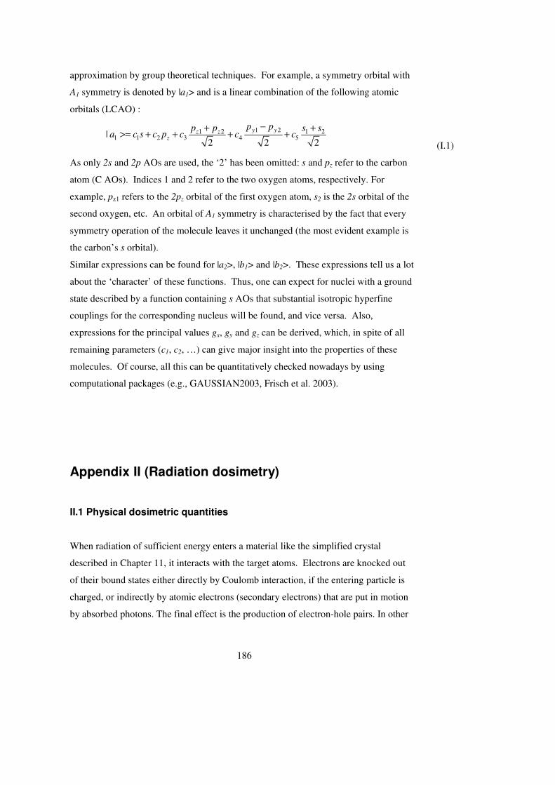
186

approximation by group theoretical techniques. For example, a symmetry orbital with

A1 symmetry is denoted by |a1> and is a linear combination of the following atomic

orbitals (LCAO) :

1 21 2 1 2

1 1 2 3 4 5|2 2 2

y yz zz

p pp p s sa c s c p c c c

−+ +>= + + + +

(I.1)

As only 2s and 2p AOs are used, the ‘2’ has been omitted: s and pz refer to the carbon

atom (C AOs). Indices 1 and 2 refer to the two oxygen atoms, respectively. For

example, pz1 refers to the 2pz orbital of the first oxygen atom, s2 is the 2s orbital of the

second oxygen, etc. An orbital of A1 symmetry is characterised by the fact that every

symmetry operation of the molecule leaves it unchanged (the most evident example is

the carbon’s s orbital).

Similar expressions can be found for |a2>, |b1> and |b2>. These expressions tell us a lot

about the ‘character’ of these functions. Thus, one can expect for nuclei with a ground

state described by a function containing s AOs that substantial isotropic hyperfine

couplings for the corresponding nucleus will be found, and vice versa. Also,

expressions for the principal values gx, gy and gz can be derived, which, in spite of all

remaining parameters (c1, c2, …) can give major insight into the properties of these

molecules. Of course, all this can be quantitatively checked nowadays by using

computational packages (e.g., GAUSSIAN2003, Frisch et al. 2003).

Appendix II (Radiation dosimetry)

II.1 Physical dosimetric quantities

When radiation of sufficient energy enters a material like the simplified crystal

described in Chapter 11, it interacts with the target atoms. Electrons are knocked out

of their bound states either directly by Coulomb interaction, if the entering particle is

charged, or indirectly by atomic electrons (secondary electrons) that are put in motion

by absorbed photons. The final effect is the production of electron-hole pairs. In other

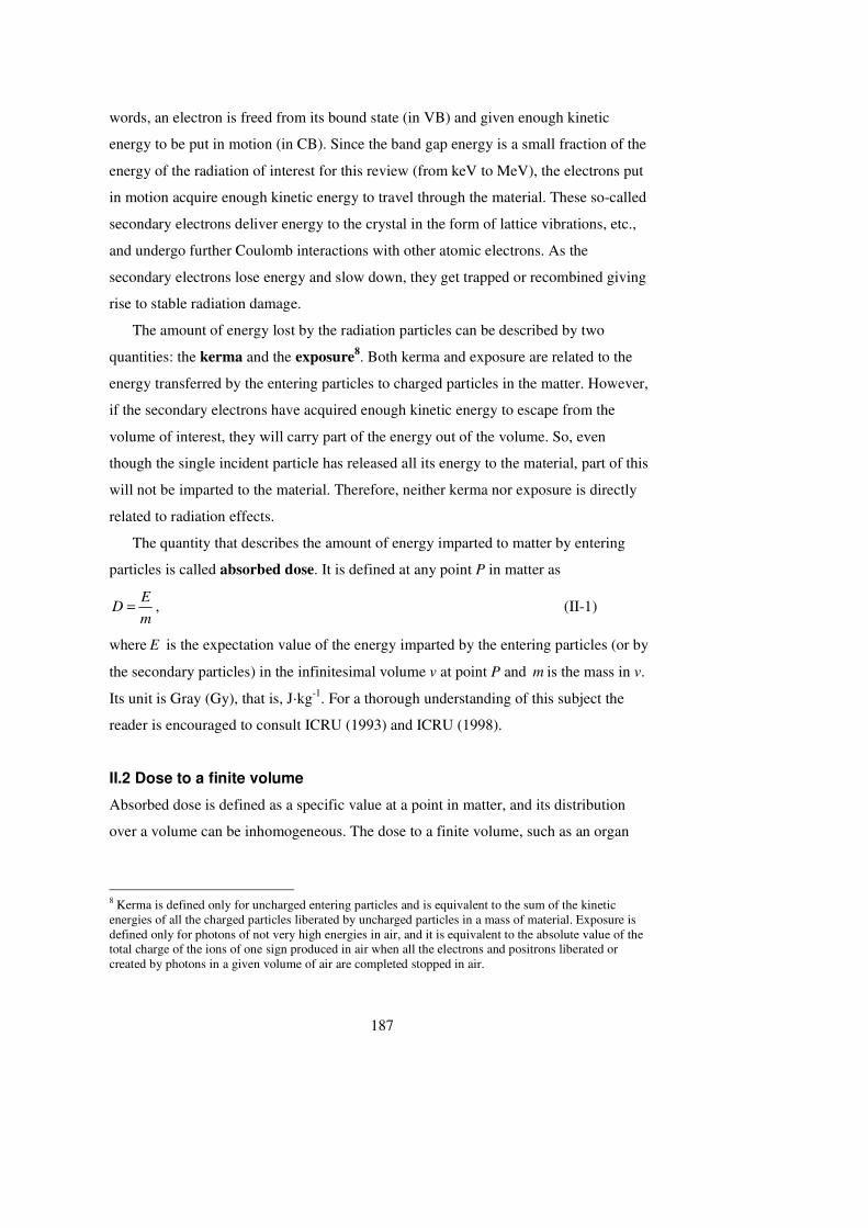
187

words, an electron is freed from its bound state (in VB) and given enough kinetic

energy to be put in motion (in CB). Since the band gap energy is a small fraction of the

energy of the radiation of interest for this review (from keV to MeV), the electrons put

in motion acquire enough kinetic energy to travel through the material. These so-called

secondary electrons deliver energy to the crystal in the form of lattice vibrations, etc.,

and undergo further Coulomb interactions with other atomic electrons. As the

secondary electrons lose energy and slow down, they get trapped or recombined giving

rise to stable radiation damage.

The amount of energy lost by the radiation particles can be described by two

quantities: the kerma and the exposure8. Both kerma and exposure are related to the

energy transferred by the entering particles to charged particles in the matter. However,

if the secondary electrons have acquired enough kinetic energy to escape from the

volume of interest, they will carry part of the energy out of the volume. So, even

though the single incident particle has released all its energy to the material, part of this

will not be imparted to the material. Therefore, neither kerma nor exposure is directly

related to radiation effects.

The quantity that describes the amount of energy imparted to matter by entering

particles is called absorbed dose. It is defined at any point P in matter as

ED

m= , (II-1)

where E is the expectation value of the energy imparted by the entering particles (or by

the secondary particles) in the infinitesimal volume v at point P and m is the mass in v.

Its unit is Gray (Gy), that is, J·kg-1. For a thorough understanding of this subject the

reader is encouraged to consult ICRU (1993) and ICRU (1998).

II.2 Dose to a finite volume

Absorbed dose is defined as a specific value at a point in matter, and its distribution

over a volume can be inhomogeneous. The dose to a finite volume, such as an organ

8 Kerma is defined only for uncharged entering particles and is equivalent to the sum of the kinetic energies of all the charged particles liberated by uncharged particles in a mass of material. Exposure is defined only for photons of not very high energies in air, and it is equivalent to the absolute value of the total charge of the ions of one sign produced in air when all the electrons and positrons liberated or created by photons in a given volume of air are completed stopped in air.

188

(e.g., a tooth), is calculated as the mean value of the absorbed dose averaged over the

volume and is expressed as

1

T

T

T m

D D dmm

= ⋅∫ , (II.2)

where mT is the mass of the finite volume and D is the absorbed dose in the mass

element dm. Calculation of this integral requires knowledge of the dose distribution

within the volume. For penetrating radiation, like high-energy photons, and relatively

small organs, like teeth, the absorbed dose distribution is sufficiently homogeneous

and, thus, the average absorbed dose is a meaningful measure of the absorbed dose. On

the other hand, for radiation with low penetration ability, like low-energy photons or

charged particles, the absorbed dose distribution within even a very small volume may

be very heterogeneous, and the average dose may not be representative of the absorbed

dose at all points of the volume.

II.3 Measurement and calculation of absorbed dose

Absorbed dose as defined at any point in matter is, in principle, a measurable quantity,

i.e., it can be determined experimentally and by computation. Experimentally, the

absorbed dose should, in principle, be measured in a small volume surrounding the

point of interest. The conditions that the volume of the dosimeter must meet in order to

be considered “small” are described by the Bragg-Gray theory. Essentially, the

dosimeter must be small enough not to perturb significantly the field of charged

particles, and such that the energy must be deposited entirely by the charged particles

crossing the volume. Ion chambers are typically designed to satisfy these conditions.

By contrast, a measurement of a dose in tooth enamel by EPR may not fulfill the

conditions of the Bragg-Gray theory in some radiation fields. In such case, the EPR

result will not represent the absorbed dose, and, again, EPR provides the mean value of

doses averaged over the tooth enamel volume.

Calculation of the absorbed dose is a difficult task. It requires the knowledge of the

radiation field at the point of the measurement, the cross sections for every possible

interaction, and the particles resulting from each process. Eq. (II-1) can be written as

189

ND E

m= ∆ , (II.3)

where N/m is the number of elementary processes per unit mass and E∆ is the

expectation value of the energy imparted in each process. The number of elementary

process per unit mass is related to the probability of interaction of a specified radiation

with matter. Depending on the radiation type (X- and γ-rays, α- and β-particles,

protons, nuclei, neutrons), the interaction with matter may occur through a variety of

processes, such as Coulomb interaction, photoelectric effect, Compton scattering,

nucleus recoil, etc. (for a detailed description of radiation interaction with crystals, see,

e.g., Knoll, 1979, pp. 40-73). Interaction of particles with target atoms is a random

process; it occurs with a probability that depends on the type and energy of radiation

and on the material. For instance, 60Co photons will predominantly interact with tooth

enamel atoms by Compton scattering; other kinds of interaction will have a negligible

probability. The probability of interaction of a specific radiation with matter is

described by an interaction coefficient, such as mass stopping power for charged

particles and mass energy-absorption coefficient for photons. In the case of

independent interaction processes with independent target atoms, the interaction

coefficient is the sum of the individual process cross sections. Cross sections are

expressed in area units (barns) and can be simplistically thought of as the cross section

of a sphere surrounding the atom: if a particle enters this sphere, the interaction occurs.

II.4 Charged particle equilibrium

Calculation of Eq. (II.3) can be simplified under the particular conditions of charged-

particle equilibrium (CPE), e.g., when the number of particles entering the volume is

the same as the number of particles leaving it (see, for instance, Johns and

Cunningham, 1983, pp. 222-224). CPE in a given material is established at a certain

depth from the surface, depending on the type and energy of the entering radiation and

on the atomic number of the irradiated material. The surface layer where CPE is not

established is called a build-up region. The depth of the build-up layer is about 4 mm

for 60Co photons in water and about 3 mm in materials similar to bone tissue (like tooth

enamel). For this reason, when irradiating a sample with a high-energy laboratory

source, such as 60Co or even 137Cs, the holder must be selected carefully, because its

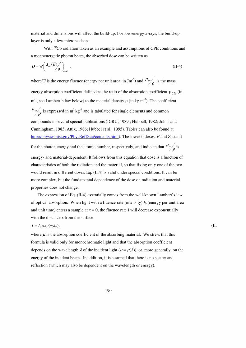
190

material and dimensions will affect the build-up. For low-energy x-rays, the build-up

layer is only a few microns deep.

With 60Co radiation taken as an example and assumptions of CPE conditions and

a monoenergetic photon beam, the absorbed dose can be written as

,

( )en

E Z

ED

µ = Ψ ρ , (II-4)

where Ψ is the energy fluence (energy per unit area, in Jm-2) and ρ

µen is the mass

energy-absorption coefficient defined as the ratio of the absorption coefficient enµ (in

m-1, see Lambert’s law below) to the material density ρ (in kg·m-3). The coefficient

ρµ

en is expressed in m2·kg-1 and is tabulated for single elements and common

compounds in several special publications (ICRU, 1989 ; Hubbell, 1982; Johns and

Cunningham, 1983; Attix, 1986; Hubbel et al., 1995). Tables can also be found at

http://physics.nist.gov/PhysRefData/contents.html). The lower indexes, E and Z, stand

for the photon energy and the atomic number, respectively, and indicate that ρ

µen is

energy- and material-dependent. It follows from this equation that dose is a function of

characteristics of both the radiation and the material, so that fixing only one of the two

would result in different doses. Eq. (II.4) is valid under special conditions. It can be

more complex, but the fundamental dependence of the dose on radiation and material

properties does not change.

The expression of Eq. (II-4) essentially comes from the well-known Lambert’s law

of optical absorption. When light with a fluence rate (intensity) I0 (energy per unit area

and unit time) enters a sample at x = 0, the fluence rate I will decrease exponentially

with the distance x from the surface:

0 exp( )I I x= −µ , (II.5)

where µ is the absorption coefficient of the absorbing material. We stress that this

formula is valid only for monochromatic light and that the absorption coefficient

depends on the wavelength λ of the incident light (µ = µ(λ)), or, more generally, on the

energy of the incident beam. In addition, it is assumed that there is no scatter and

reflection (which may also be dependent on the wavelength or energy).

191

Using Lambert’s law, it is easy to derive that the absorbed intensity and energy

behave similarly as a function of sample thickness d:

(1 )dabs 0E = E e

−µ− (II.6)

The relation between E0 and I0 is simple:

0 0E I A t= ∆ . (II.7)

A and ∆t denote the surface area and the duration of the exposure to the

light,respectively.

When the absorption of the light is weak, mathematically expressed by µ<<1/d, the

exponential in Eq. (II.6) can be approximated by a linear function, leading to

0absE E d= µ . (II.8)

The absorbed dose Dabs is then

00

abs absabs

E E ED I t

m V A

µ µ= = = = ∆

ρ ρ ρ. (II.9)

This expression makes it quite clear that the absorbed dose depends on both the energy

of the incident beam (via µ) and the absorbing material (via ρ), even if the total incident

energy per unit area (or the fluence) were the same. In this simple form, the absorbed

dose is the product of the energy fluence and the mass-absorption coefficient defined as

µ/ρ.

Appendix III (Uncertainty in measurements)

The terminology and formalism used in Chapter 17, which deals with the sources of

uncertainties in dose in tooth enamel, are based on "Guide to the expression of

uncertainty in measurement", the so called GUM (ISO, 1995)9. This guide has

introduced important changes in the traditional way of expressing uncertainties. Since

it is probably not very well known to people unfamiliar with metrology, it may be

useful to review some of the most important concepts.

9 The basis of this guide is CIPM Recommendation 1 (CI-1981), which is the only recommendation concerning the expression of uncertainty in measurement endorsed by an intergovernmental organization. The Guide mentioned here was developed jointly by ISO, IEC, OIML and BIPM; therefore, it can often be found with a different reference (for example BIPM 1993).

192

It is well known that the result of a measurement is an approximation or estimate of

the (true10) value of the measurand (i.e., the quantity to be measured). The difference

between the measurement result and the value of the measurand is the error of the

measurement, caused by unavoidable imperfections in the measurement procedure.

The error is generated by random and systematic effects of influence quantities (such as

room temperature or sample mass) on the measurement result. Random effects are

related to stochastic variations of the influence quantities and can be reduced by

increasing the number of observations. Systematic effects can instead be reduced by

application of corrections or correction factors to the measurement result, once the

systematic effect has been recognized. If an effect is not recognized as systematic, it

may contribute to the error as a random effect. An example is the dependence of a

measurement on room temperature. The result of the measurement can be corrected if

its trend with temperature is known and if the temperature is monitored; otherwise, the

fluctuations of the measurement result due to the random temperature variations will

contribute as a random effect.

Since the value of the measurand is unknowable, the error of the measurement is

unknowable as well, and, so, the corrections are imperfect. Consequently, the corrected

result of the measurand “is still only the best estimate of the value of the measurand,

because of the uncertainty arising from the random effects and from imperfect

correction of the result for systematic effects." (ISO, 1995). The lack of exact

knowledge of the value of the measurand is taken into account by associating

uncertainty of the measurement to the corrected result, which, in the GUM

terminology, is a parameter characterizing the dispersion of the values that could

reasonably be attributed to the measurand.

According to the GUM formalism, the first step in evaluating the uncertainty of a

measurement result Y is to determine a mathematical model, with the estimated values

of a, b, …, n of the input quantities A, B, …N:

Y = f(a, b, . . . , n). (III-1)

The function f in Eq.(III-1) describes the measurement process, and it should contain,

in particular, all the influence quantities that can contribute a significant uncertainty to

the measurement result (for this reason, they are also called sources of uncertainties).

10 The word “true” is now considered redundant; it is not recommended for use any more (ISO 1995).

193

For example, the input quantities are all the sources of variability due to the observer,

instrument, sample, room conditions, times of observation. Efforts should always be

made to recognize and quantify all possible influence quantities. In particular, every

effort should be made to recognize systematic effects. In fact, as stated in the ISO

recommendations, “It is assumed that the result of a measurement has been corrected

for all recognized significant systematic effects.”. Therefore, a result of a measurement

must be presented as a corrected result of the measurement, corr

Y . For example, if a

measurement is affected by both corrections and correction factors, Eq.(IV-1) can be

written as:

( , , ) ( )= × +∑∏N M

corr i i k i i k

ki

Y x F C f x F C , (III-2)

where xi are values of the input quantities (a, b, …, n), iF are correction factors

(multiplicative) and k

C are corrections (additive).

Uncertainty of a corrected result of a measurement is determined by the law of

propagation of the uncertainty of the input estimates and is called the combined

uncertainty (assuming that the input variables are not correlated) (ISO, 1995, pp. 46-

47):

1 1

22 2 22 2

2 2 2 2 2 2 2

corr 1 N 1 M

N M

f f f f f fu(Y ) = u(a) +... + u(n) + u(F ) +...+ u(F ) + u(C ) +...+ u(C )

a n F F C C

∂ ∂ ∂ ∂ ∂ ∂ ∂ ∂ ∂ ∂ ∂ ∂

(III.3)

where u(a), u(b) and u(c) are the standard uncertainties of a, b and c. The standard

uncertainty of a measured value is expressed as an estimated standard deviation, i.e., a single

sigma uncertainty.

As the uncertainty in Ycorr is associated with imperfect knowledge of random and

systematic effects, the uncertainties associated to the two classes of effects were

formerly reported separately. One of the changes introduced by the GUM in the

traditional way of expressing uncertainties is that the two components are treated in

exactly the same way and combined into single uncertainty. Instead, the terms of

uncertainty are categorized according to the method that they are evaluated with,

independently from their random or systematic nature. They are then divided into

uncertainties of Type A and Type B. Uncertainties of Type A are evaluated based on

statistical analysis of a series of observations, while uncertainties of Type B are

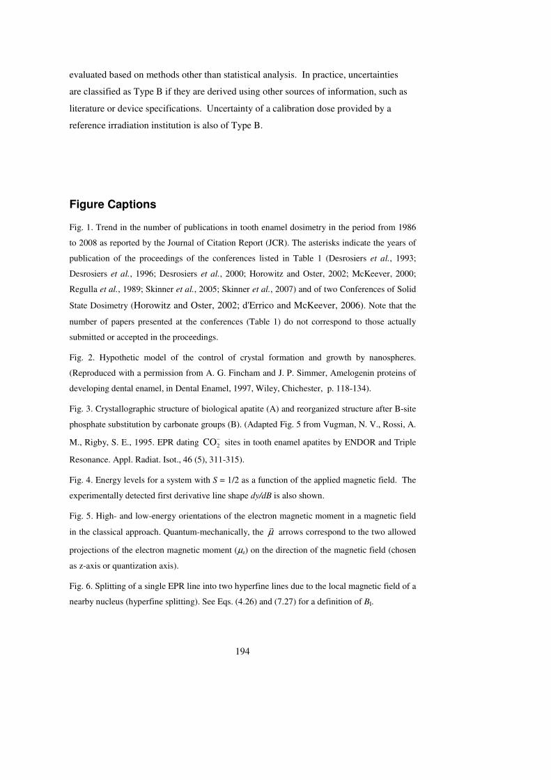
194

evaluated based on methods other than statistical analysis. In practice, uncertainties

are classified as Type B if they are derived using other sources of information, such as

literature or device specifications. Uncertainty of a calibration dose provided by a

reference irradiation institution is also of Type B.

Figure Captions

Fig. 1. Trend in the number of publications in tooth enamel dosimetry in the period from 1986

to 2008 as reported by the Journal of Citation Report (JCR). The asterisks indicate the years of

publication of the proceedings of the conferences listed in Table 1 (Desrosiers et al., 1993;

Desrosiers et al., 1996; Desrosiers et al., 2000; Horowitz and Oster, 2002; McKeever, 2000;

Regulla et al., 1989; Skinner et al., 2005; Skinner et al., 2007) and of two Conferences of Solid

State Dosimetry (Horowitz and Oster, 2002; d'Errico and McKeever, 2006). Note that the

number of papers presented at the conferences (Table 1) do not correspond to those actually

submitted or accepted in the proceedings.

Fig. 2. Hypothetic model of the control of crystal formation and growth by nanospheres.

(Reproduced with a permission from A. G. Fincham and J. P. Simmer, Amelogenin proteins of

developing dental enamel, in Dental Enamel, 1997, Wiley, Chichester, p. 118-134).

Fig. 3. Crystallographic structure of biological apatite (A) and reorganized structure after B-site

phosphate substitution by carbonate groups (B). (Adapted Fig. 5 from Vugman, N. V., Rossi, A.

M., Rigby, S. E., 1995. EPR dating −2CO sites in tooth enamel apatites by ENDOR and Triple

Resonance. Appl. Radiat. Isot., 46 (5), 311-315).

Fig. 4. Energy levels for a system with S = 1/2 as a function of the applied magnetic field. The

experimentally detected first derivative line shape dy/dB is also shown.

Fig. 5. High- and low-energy orientations of the electron magnetic moment in a magnetic field

in the classical approach. Quantum-mechanically, the µ�

arrows correspond to the two allowed

projections of the electron magnetic moment (µz) on the direction of the magnetic field (chosen

as z-axis or quantization axis).

Fig. 6. Splitting of a single EPR line into two hyperfine lines due to the local magnetic field of a

nearby nucleus (hyperfine splitting). See Eqs. (4.26) and (7.27) for a definition of BI.

195

Fig. 7. EPR spectrum of Mn2+ in MgO featuring the six-lines hyperfine structure due to I = 5/2.

The smaller additional line around 354 mT does not belong to the Mn2+ spectrum.

Fig. 8. (a) Variation of the EPR resonance field for an axial defect when the magnetic field is

rotated in an arbitrary plane containing the symmetry axis from the parallel orientation (0°, B =

hν/g//β)) to the perpendicular orientation (90°, B = hν/g⊥β). The powder spectrum is also shown

in the bottom. (b) EPR spectra of an axial defect when it is rotated about the symmetry axis (B

= hν/g⊥β). Considering both angular variations, one can understand that the perpendicular

feature in the powder spectrum (lowest curve in the left part) contains contributions from many

more orientations and is much stronger than the parallel one.

Fig. 9. Illustration of site splitting in the case of four-fold symmetry (symbolized by the central

square). Paramagnetic Defect 1 (arrow) is multiplicated by rotations over 90° (2), 180° (3) and

270° (4). Defects 1 to 4 are physically equivalent (note that they can be translated and are not

necessarily centered, as in the figure). When a magnetic field is applied at an angle α, the pairs

(1,3) and (2,4) will become unequivalent. Two different EPR lines will result from the site

splitting. At α = 45°, only one line will be visible.

Fig. 10. Orthorhombic powder spectrum (gx = 2.003; gy = 2.000 ; gz = 1.997). The microwave

frequency used in the simulation is 9.50 GHz.

Fig. 11. Angular variation (steps of 10°) of the EPR spectrum of heated tooth enamel plates at

34 GHz (Q-band). The main signals are due to a single CO2- radical. In the upper spectra, the

magnetic field is oriented (nearly) parallel to the macroscopic enamel surface; in the lower

spectra, the field is perpendicular to the surface. (This shows that most radicals have their O-O

(gy = 1.997) axes along this perpendicular direction).

Fig. 12. Effect of frequency renormalization to 9.47 GHz. Spectrum 1 was originally recorded at

9.39 GHz, whereas Spectrum 2 was taken at 9.18 GHz. The features indicated by the arrows are

artificially and incorrectly shifted by the normalization because hyperfine interactions next to

the g-factor determine these positions. The positions of the features that are controlled only by

g-anisotropy are perfectly aligned after normalization (connected by the dashed lines).

Fig. 13. Illustration of a possible wrong relative g-value assignment (graphical estimation would

lead to gx1 > gx2, whereas the calculation using a Lorentzian line shape was done with gx1 < gx2)

Parameters of the curve a (CO33- in calcite): gx1 = 2.0031, gy1 = 2.0031, gz1 = 2.0013, C = 2.5.

Parameters of the curve b (CO2-): gx2 = 2.0032, gy2 = 2.0016, gz2 = 1.9973, C = 2.5.

196

Fig. 14. An EPR spectrum of a paramagnetic center with an orthorhombic g-tensor (gx = 2.0038,

gy = 2.0024, gz = 2.0010, CL = 2.5; the parameters are typical for CO33-).

Fig. 15. An EPR spectrum of a paramagnetic center with an axial g-tensor (gx = gy = 2.0032, gz

= 1.9973, CL = 2.5; the parameters are typical for CO2-).

Fig. 16. An EPR spectrum of a paramagnetic center with an orthorhombic g-tensor and

(a) a Gaussian line shape (gx = 2.0032, gy = 1.9973, gz = 2.0016, CG = 2.5)

(b) a Lorentzian line shape (same parameters)

Fig. 17. Fitting of a powder spectrum of tooth enamel recorded several months after irradiation

at 10 mW (the dotted and solid lines correspond to the experimental and fitted curves,

respectively). A Lorentzian line shape was used with gx = 2.0030, gy = 1.9971 ; gz = 2.0018.

The g markers 1-8 cover the g range between 2.0043 and 1.9958. The microwave frequency is

9.3 GHz.

Fig. 18. A diagram of energy levels and transitions used in ENDOR (M and m denote the

electron and nuclear spin quantum numbers). In an ENDOR experiment, an EPR transition

(1↔3 or 2↔4) is saturated with a microwave field, while a radiation frequency field is applied

simultaneously to induce an NMR or ENDOR transition (1↔2 or 3↔4).

Fig. 19. Schematic proton ENDOR spectrum with the larger matrix ENDOR line near 15 MHz.

Fig. 20. A typical EPR spectrum of human tooth enamel irradiated to 0.4 Gy (top) and 1 Gy

(bottom). The calculated isotropic-looking native signal around g = 2.0045 and the quasi-axial

(orthorhombic) dosimetric signal (g-factor range 2.003 – 1.997) are shown in the upper

spectrum (dashed lines). The ratio of the amplitudes of the two signals depends on the

parameters used in the spectrum acquisition. The two symmetric lines at the spectrum edges are

the 3rd and the 4th lines of the EPR spectrum of a Mn2+/MgO reference sample present in the

cavity.

Fig. 21. Symmetry axes of CO2-

Fig. 22. Molecular orbitals of CO2-. The carbon and the (two) oxygen atomic levels/orbitals

making up the molecular orbitals of the molecular ion are shown on the left and the right side,

respectively. All 2CO−

levels can be split only by a magnetic field.

Fig. 23. (a) EPR spectra of an enamel block recorded at 10 mW with �B perpendicular to the

enamel surface. Solid curves show the spectrum recorded without heating; dotted curves show

197

the spectrum with preheating. (b) Same as (a) at 0.1 mW. (c) Same as (a) for �B parallel to the

enamel surface. (d) Same as (c) at 0.1 mW. In (e)-(h), the solid curves are the same as in (a)-

(d). The dotted curves in (e)-(h) are the sums of the corresponding dotted curves of (a)-(d) and

a typical powder spectrum (see, e.g., Fig. 16 or 17 in Chapter 5). In the related spectrum pairs

(e),(g) and (f),(h), the same multiplication factor for the powder spectrum has been used.

Fig. 24. EPR spectrum of heated tooth enamel. 400 °C (a – b); 1000 °C (d). Microwave

power: 64 mW (a); 1 mW (b). Curve c is a calculated spectrum of the septet-quartet signal on

Curve b. The two symmetric lines in the opposite phase on Curve a are the 3rd and 4th lines of

an external Mn2+ marker located at the bottom of the cavity.

Fig. 25. EPR spectrum of a tooth enamel powder prepared with a low-speed power-driven saw

without water cooling (dotted line), compared with the spectrum of the untreated half of the

same sample (solid line). Arrows A and B indicate two features induced by the mechanical

treatment.

Fig. 26. The native signal in the EPR spectra of: (a) fossil tooth (200 Gy, 2 mW); (b) frog leg

(~1 kGy, 12.5 mW); (c) human tooth enamel (not intentionally irradiated, 10 mW) ; (d)

synthetic apatite (~10 kGy, 0.1 mW) (Callens et al., 1998)

Fig. 27. Typical parasitic signals in the EPR spectra of three different unirradiated tooth enamel

samples (a, b, c). The arrows indicate the parasitic signals. The two symmetric lines are the 3rd

and 4th lines of an external Mn2+ marker.

Fig. 28. Band diagram of a solid showing electron (e-, 1) and hole (h+, 2) trapping and electron-

hole recombination (3) after an electron-hole pair (e-,h+) was created by ionizing radiation with

sufficient energy hν.

Fig. 29. Hypothetical dose-response curve in the case of a competing trap (N1 > N2 ; S2 > S1 ;

Dsat1 > Dsat2).

Fig. 30. Aspect of tooth enamel powder with 0.5-1-mm grains.

Fig. 31. Flow diagram of a typical tooth enamel preparation procedure. The average time of

each step is shown only where it exceeds 15 min. For the dentin/enamel chemical separation,

the duration of 45-60 min was obtained by dividing the total time (15 h) by the typical number

of teeth prepared in parallel (about 15). The estimated total time is about 20 h per tooth for a

trained operator.

Fig. 32. Block diagram of a typical X-band EPR spectrometer.

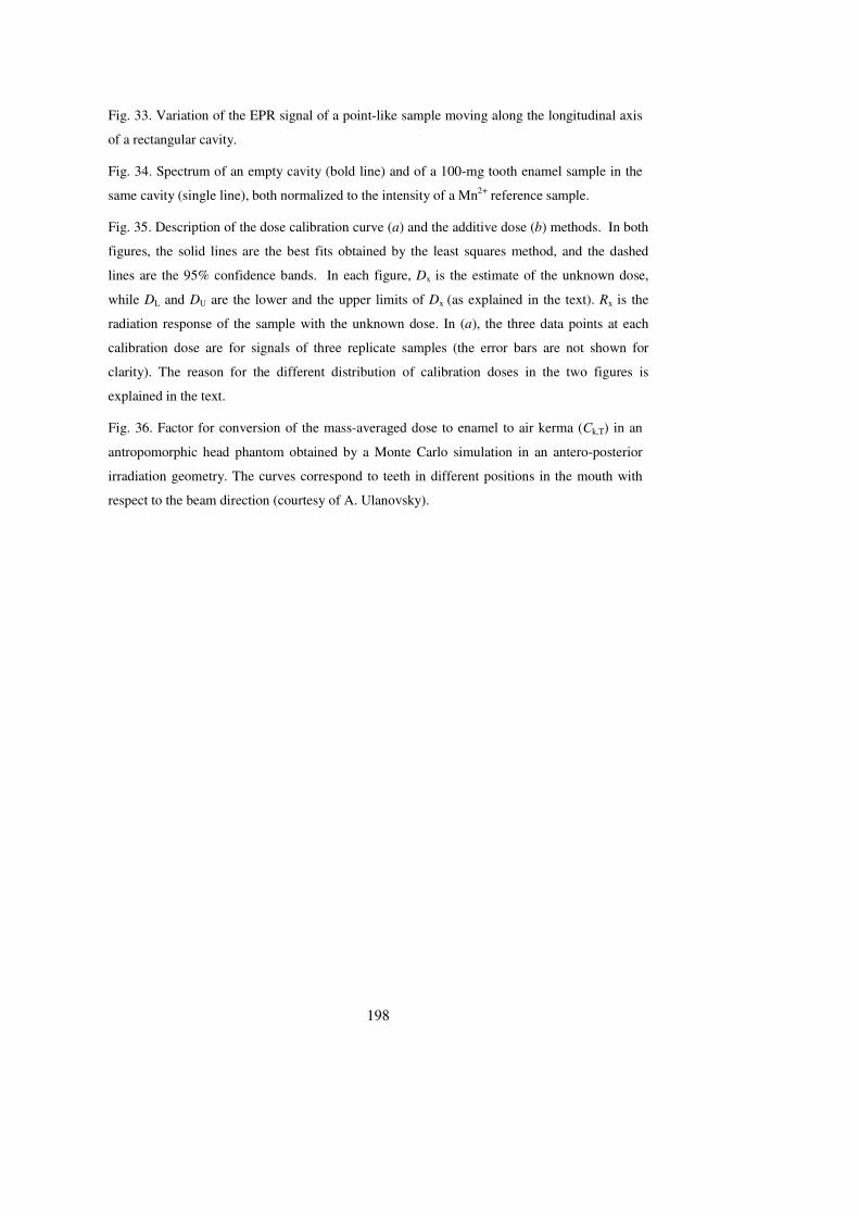
198

Fig. 33. Variation of the EPR signal of a point-like sample moving along the longitudinal axis

of a rectangular cavity.

Fig. 34. Spectrum of an empty cavity (bold line) and of a 100-mg tooth enamel sample in the

same cavity (single line), both normalized to the intensity of a Mn2+ reference sample.

Fig. 35. Description of the dose calibration curve (a) and the additive dose (b) methods. In both

figures, the solid lines are the best fits obtained by the least squares method, and the dashed

lines are the 95% confidence bands. In each figure, Dx is the estimate of the unknown dose,

while DL and DU are the lower and the upper limits of Dx (as explained in the text). Rx is the

radiation response of the sample with the unknown dose. In (a), the three data points at each

calibration dose are for signals of three replicate samples (the error bars are not shown for

clarity). The reason for the different distribution of calibration doses in the two figures is

explained in the text.

Fig. 36. Factor for conversion of the mass-averaged dose to enamel to air kerma (Ck,T) in an

antropomorphic head phantom obtained by a Monte Carlo simulation in an antero-posterior

irradiation geometry. The curves correspond to teeth in different positions in the mouth with

respect to the beam direction (courtesy of A. Ulanovsky).

199

Table 1. Overview of the tooth dosimetry content of the seven conferences on EPR

dosimetry (Desrosiers et al., 1993; Desrosiers et al., 1996; Desrosiers et al., 2000;

Regulla et al., 1989; Skinner et al., 2005).

Conference

No.*

Year Location Number of papers on tooth dosimetry

presented at the conference

1 1985 Ube-Akiyoshi (Japan) 3

2 1988 Neuherberg (Germany) 3

3 1991 Gaithersburg (US, MD) 3

4 1995 Neuherberg (Germany) 13

5 1998 Obninsk (Russia) 17

6 2003 Sao Paulo (Brasil) 14

7 2006 Bethesda (US, MD) 32

8 2008 Hanover (US, NH) **

*Title varies. **Proceedings were not published yet when this review was printed

200

Table 2. Chronology of development of human dentition (adapted from IAEA, 2002).

Tooth First evidence of calcification

Enamel completed

Central incisor 4 mo. in utero 1.5 mo.

Lateral incisor 4.5 mo. in utero 2.5 mo.

Canine 5 mo. in utero 9 mo.

First molar 5 mo. in utero 6 mo.

Maxillary

Second molar 6 mo. in utero 11 mo.

Central incisor 4.5 mo. in utero 2.5 mo.

Lateral incisor 4.5 mo. in utero 3 mo.

Canine 5 mo. in utero 9 mo.

First molar 5 mo. in utero 5.5 mo.

Primary dentition

Mandibular

Second molar 6 mo. in utero 10 mo.

Central incisor 3-4 mo. 4-5 yr.

Lateral incisor 10-12 mo. 4-5 yr.

Canine 4-5 mo. 6-7 yr.

First premolar 1.5-1.75 yr. 5-6 yr.

Second premolar 2-2.25 yr. 6-7 yr.

First molar At birth 2.5-3 yr.

Second molar 2.5-3 yr. 7-8 yr.

Maxillary

Third (wisdom) molar 7-9 yr. 12-16 yr.

Central incisor 3-4 mo. 4-5 yr.

Lateral incisor 3-4 mo. 4-5 yr.

Canine 4-5 mo. 6-7 yr.

First premolar 1.75-2 yr. 5-6 yr.

Second premolar 2.25-2.5 yr. 6-7 yr.

First molar At birth 2.5-3 yr.

Second molar 2.5-3 yr. 7-8 yr.

Permanent dentition

Mandibular

Third(wisdom) molar 8-10 yr. 12-16 yr.

20

Table 3. Major and minor constituents of tooth enamel (dry weight) (Adapted Table 8.2, from

Driessens and Verbeeck, 1990, p. 107).

Constituent Average concentration (dry weight %)

Ca 36.6

P 17.7

CO3 3.2

Na 0.67

Mg 0.35

Cl 0.35

K 0.04

20

Table 4. Trace elements in tooth enamel (Adapted Table 8.4 from Driessens and Verbeeck, 1990, p.

111).

Element Mean concentration (µg/g, dry weight)

Zn 179

Sr 156

Si 136

F 120

S 59

Al 51

Fe 33

20

Table 5. Spin Hamiltonian parameters of carbonate-derived radicals in several materials (13C

hyperfine parameters are in MHz). HAp = Hydroxyapatite; sc = single crystal; po = powder.

Radical Host gx gy gz giso Ax Ay Az Aiso Ref.

CO2- NaHCO2 2.0032 1.9975 2.0014 2.0006 436 422 546 468 a

CaCO3 2.0032 1.9972 2.0016 2.0006 379 369 496 415 b

HAp, sc 2.0027 1.9974 2.0027 2.0009 c

KCl 2.0025 1.9959 2.0025 2.0003 388 328 388 368 d

MgO 2.0030 1.9970 2.0015 2.0005 513 506 630 550 e

HaA, po 2.0006 410 f

Hap, po 2.0030 1.9970 2.0015 2.0005 460 556 445 487 f

O-CO- MgO 2.0035 1.9970 2.0028 2.0011 485 478 600 521 e

CO33- CaCO3 2.0031 2.0031 2.0013 2.0025 312 312 480 368 g

Y-CO33- CaCO3 2.0024 2.0038 2.0012 2.0025 353 354 528 412 h

Li-CO33- CaCO3 2.0031 2.0031 2.0012 2.0025 354 354 i

CO3- CaCO3 2.0162 2.0162 2.0051 2.0125 26.5 26.5 36.8 29.9 g

CaCO3 2.0132 2.0194 2.0055 2.0127 j

KHCO3 2.0086 2.0184 2.0066 2.0112 28.1 28.3 39.3 31.9 k

CO- MgO 2.0055 2.0055 2.0021 2.0044 75.8 30.9 0 35.6 l

Hap, po 2.0061 2.0061 2.0019 2.0047 m

Hap, po 2.0058 2.0041 2.0023 2.0041 n

aOvenall and Whiffen, 1961; bMarshall et al., 1964; cVanhaelewyn et al., 2000b; dCallens et al., 1989a; eMeriaudeau et al., 1975; fCallens et al., 1989b; gSerway and Marshall, 1967a; hMarshall and McMillan., 1968; iBacquet et al., 1975; jSerway and Marshall, 1967b; kChantry et al., 1962; lLunsford and Jayne, 1966; mSchramm and Rossi, 1999; nMoens et al., 1991.

20

Table 6. Carbonate-derived radicals interacting with a proton (13C hyperfine parameters are in

MHz).

Radical Host gx gy gz giso Ax Ay Az Aiso Ref

CO2(H) KHCO3 2.0031 1.9971 2.0012 2.0005 397 372 501 423 a

HCO32- CaCO3 2.0050 2.0039 2.0020 2.0036 126 100 78 101 b

HCO- HAp-po 2.0061 2.0061 2.0019 2.0047 188 188 373 250 c

aChantry and Whiffen, 1962 (13C hyperfine and g-tensor axes are non-coincident). bCass et al., 1974 (hyperfine values are due to 1H). cSchramm and Rossi, 1999 (hyperfine values are due to 1H).

20

Table 7. Main properties of the EPR signals induced in tooth enamel by mechanical operations

Tool Mechanism Induced signal Affecting factors Fading Comments

Mortar

and pestle

Load Undistinguishable from the

native signal a, b, c, d, e

Grinding time

(i.e., grain size) b,

c, d

48 h c Removal of the induced

centers by etching c

Press Load Not investigated in enamel Not investigated

in enamel

Not investigated

in enamel

There is evidence of formation

of a signal close to the native

signal in dentin f

Drill Friction giso=2.002; ∆B=0.08 mT a, e, g Water

refrigeration g

No fading

reported

Similarity of the mechanically

and thermally induced signals

e, g, h.

Saw Friction giso=2.002; ∆B=0.08 mT g Water

refrigeration g

No fading

reported

Similarity of the mechanically

and thermally (1000 °C)

induced signals g

a) Desrosiers et al., 1989; b) Polyakov et al., 1995; c) Fattibene et al., 1998; d) Sholom et al., 1998a; e)

Kirillov et al., 2002; f) Fattibene et al., 2006; g) Aragno et al., 2001; h) Aldrich et al., 1992.

Met opmaak: Engels

(Groot-Brittannië)

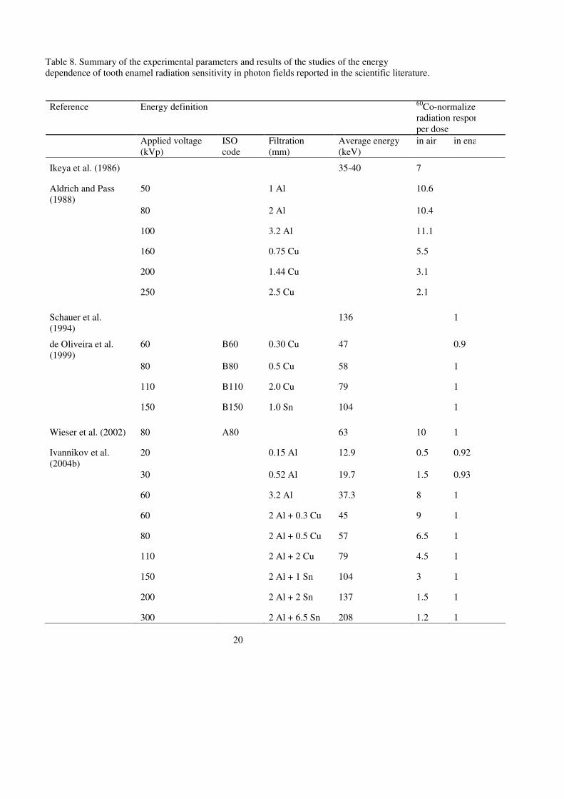
20

Table 8. Summary of the experimental parameters and results of the studies of the energy dependence of tooth enamel radiation sensitivity in photon fields reported in the scientific literature.

Reference Energy definition 60Co-normalized radiation response per dose

Applied voltage (kVp)

ISO code

Filtration (mm)

Average energy (keV)

in air in enamel

Ikeya et al. (1986) 35-40 7

Aldrich and Pass (1988)

50 1 Al 10.6

80 2 Al 10.4

100 3.2 Al 11.1

160 0.75 Cu 5.5

200 1.44 Cu 3.1

250 2.5 Cu 2.1

Schauer et al. (1994)

136 1

de Oliveira et al. (1999)

60 B60 0.30 Cu 47 0.9

80 B80 0.5 Cu 58 1

110 B110 2.0 Cu 79 1

150 B150 1.0 Sn 104 1

Wieser et al. (2002) 80 A80 63 10 1

Ivannikov et al. (2004b)

20 0.15 Al 12.9 0.5 0.92

30 0.52 Al 19.7 1.5 0.93

60 3.2 Al 37.3 8 1

60 2 Al + 0.3 Cu 45 9 1

80 2 Al + 0.5 Cu 57 6.5 1

110 2 Al + 2 Cu 79 4.5 1

150 2 Al + 1 Sn 104 3 1

200 2 Al + 2 Sn 137 1.5 1

300 2 Al + 6.5 Sn 208 1.2 1

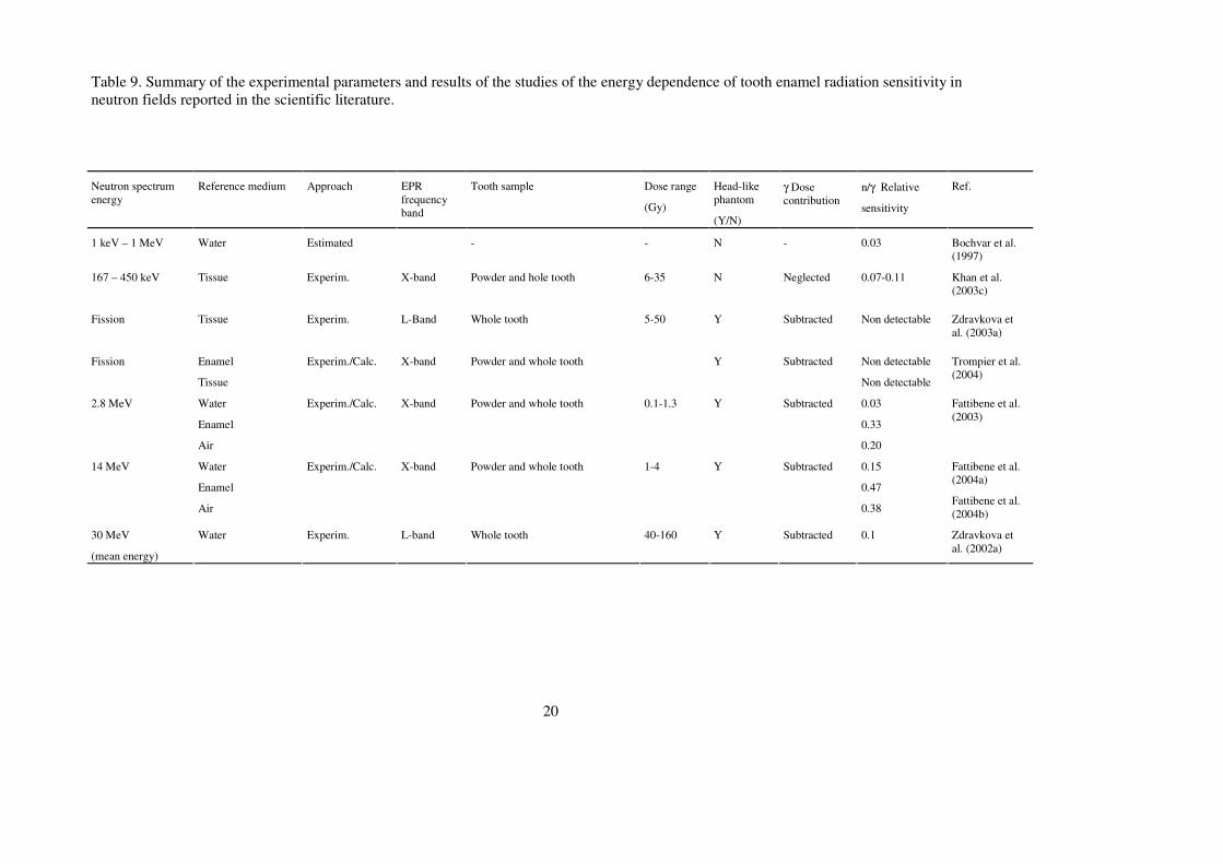
20

Table 9. Summary of the experimental parameters and results of the studies of the energy dependence of tooth enamel radiation sensitivity in neutron fields reported in the scientific literature.

Neutron spectrum energy

Reference medium Approach EPR frequency band

Tooth sample Dose range

(Gy)

Head-like phantom

(Y/N)

γ Dose contribution

n/γ Relative

sensitivity

Ref.

1 keV – 1 MeV Water Estimated - - N - 0.03 Bochvar et al. (1997)

167 – 450 keV Tissue Experim.

X-band Powder and hole tooth 6-35 N Neglected 0.07-0.11 Khan et al. (2003c)

Fission Tissue Experim.

L-Band Whole tooth 5-50 Y Subtracted Non detectable Zdravkova et al. (2003a)

Fission Enamel

Tissue

Experim./Calc.

X-band Powder and whole tooth Y Subtracted Non detectable

Non detectable

Trompier et al. (2004)

2.8 MeV Water

Enamel

Air

Experim./Calc. X-band Powder and whole tooth 0.1-1.3 Y Subtracted 0.03

0.33

0.20

Fattibene et al. (2003)

14 MeV Water

Enamel

Air

Experim./Calc. X-band Powder and whole tooth 1-4 Y Subtracted 0.15

0.47

0.38

Fattibene et al. (2004a)

Fattibene et al. (2004b)

30 MeV

(mean energy)

Water Experim.

L-band Whole tooth 40-160 Y Subtracted 0.1 Zdravkova et al. (2002a)

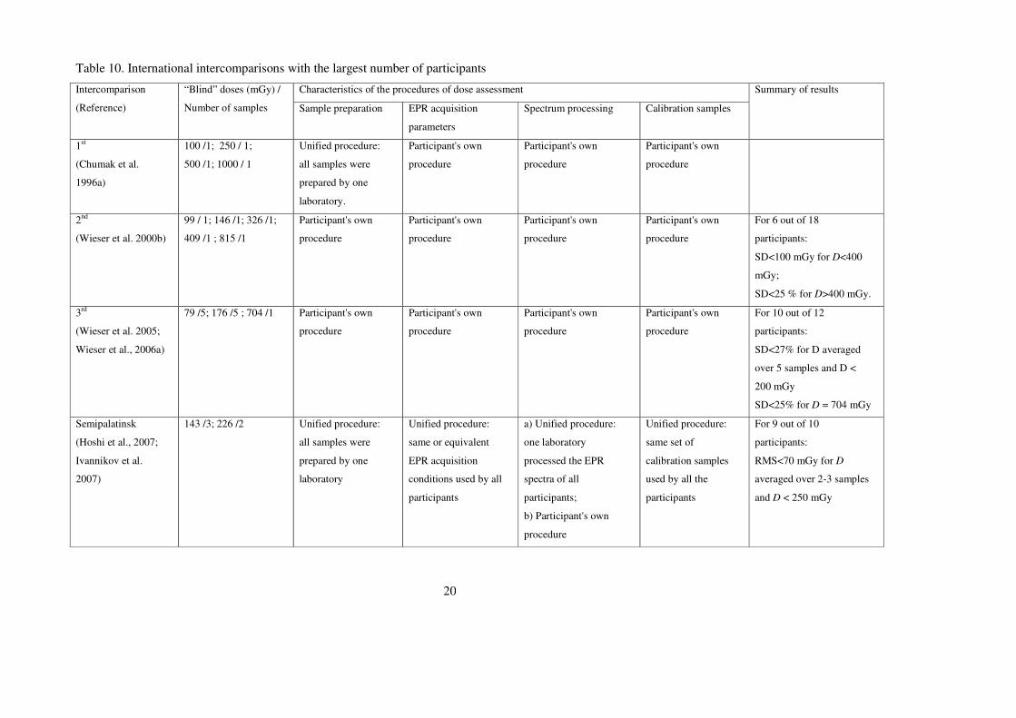
20

Table 10. International intercomparisons with the largest number of participants

Characteristics of the procedures of dose assessment Intercomparison

(Reference)

“Blind” doses (mGy) /

Number of samples Sample preparation EPR acquisition

parameters

Spectrum processing Calibration samples

Summary of results

1st

(Chumak et al.

1996a)

100 /1; 250 / 1;

500 /1; 1000 / 1

Unified procedure:

all samples were

prepared by one

laboratory.

Participant's own

procedure

Participant's own

procedure

Participant's own

procedure

2nd

(Wieser et al. 2000b)

99 / 1; 146 /1; 326 /1;

409 /1 ; 815 /1

Participant's own

procedure

Participant's own

procedure

Participant's own

procedure

Participant's own

procedure

For 6 out of 18

participants:

SD<100 mGy for D<400

mGy;

SD<25 % for D>400 mGy.

3rd

(Wieser et al. 2005;

Wieser et al., 2006a)

79 /5; 176 /5 ; 704 /1 Participant's own

procedure

Participant's own

procedure

Participant's own

procedure

Participant's own

procedure

For 10 out of 12

participants:

SD<27% for D averaged

over 5 samples and D <

200 mGy

SD<25% for D = 704 mGy

Semipalatinsk

(Hoshi et al., 2007;

Ivannikov et al.

2007)

143 /3; 226 /2 Unified procedure:

all samples were

prepared by one

laboratory

Unified procedure:

same or equivalent

EPR acquisition

conditions used by all

participants

a) Unified procedure:

one laboratory

processed the EPR

spectra of all

participants;

b) Participant's own

procedure

Unified procedure:

same set of

calibration samples

used by all the

participants

For 9 out of 10

participants:

RMS<70 mGy for D

averaged over 2-3 samples

and D < 250 mGy

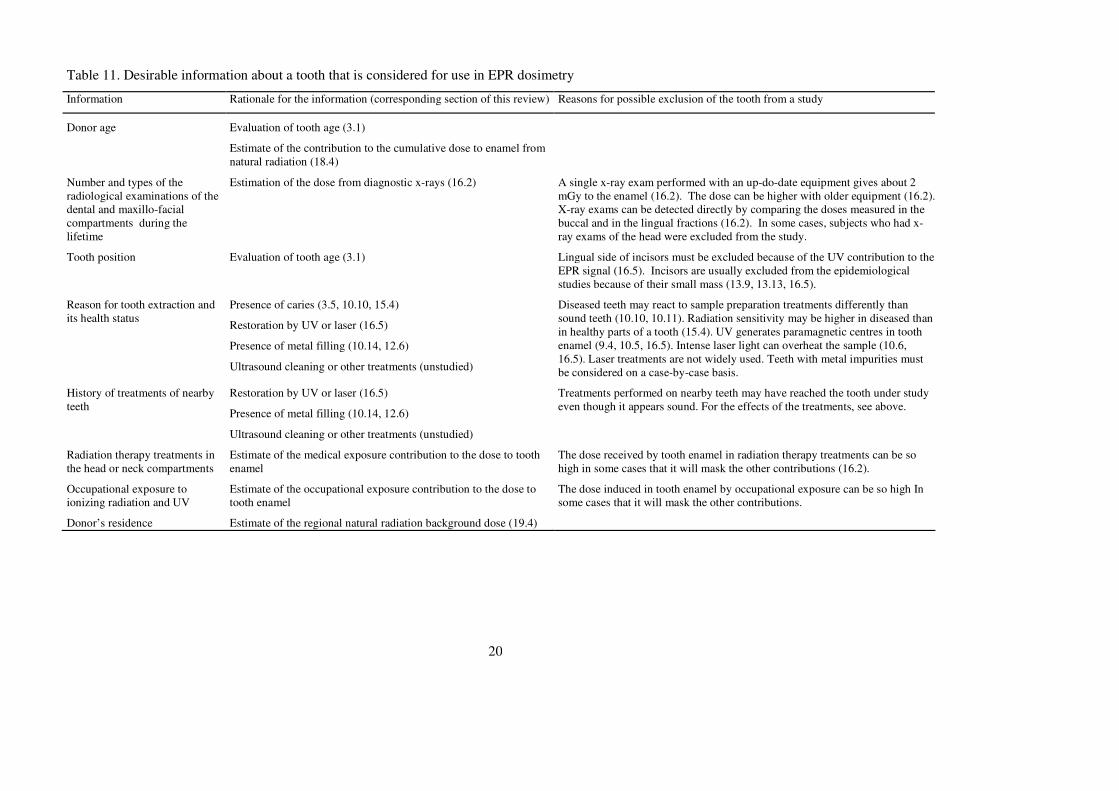
20

Table 11. Desirable information about a tooth that is considered for use in EPR dosimetry

Information Rationale for the information (corresponding section of this review) Reasons for possible exclusion of the tooth from a study

Donor age Evaluation of tooth age (3.1)

Estimate of the contribution to the cumulative dose to enamel from natural radiation (18.4)

Number and types of the radiological examinations of the dental and maxillo-facial compartments during the lifetime

Estimation of the dose from diagnostic x-rays (16.2)

A single x-ray exam performed with an up-do-date equipment gives about 2 mGy to the enamel (16.2). The dose can be higher with older equipment (16.2). X-ray exams can be detected directly by comparing the doses measured in the buccal and in the lingual fractions (16.2). In some cases, subjects who had x-ray exams of the head were excluded from the study.

Tooth position Evaluation of tooth age (3.1)

Lingual side of incisors must be excluded because of the UV contribution to the EPR signal (16.5). Incisors are usually excluded from the epidemiological studies because of their small mass (13.9, 13.13, 16.5).

Reason for tooth extraction and its health status

Presence of caries (3.5, 10.10, 15.4)

Restoration by UV or laser (16.5)

Presence of metal filling (10.14, 12.6)

Ultrasound cleaning or other treatments (unstudied)

Diseased teeth may react to sample preparation treatments differently than sound teeth (10.10, 10.11). Radiation sensitivity may be higher in diseased than in healthy parts of a tooth (15.4). UV generates paramagnetic centres in tooth enamel (9.4, 10.5, 16.5). Intense laser light can overheat the sample (10.6, 16.5). Laser treatments are not widely used. Teeth with metal impurities must be considered on a case-by-case basis.

History of treatments of nearby teeth

Restoration by UV or laser (16.5)

Presence of metal filling (10.14, 12.6)

Ultrasound cleaning or other treatments (unstudied)

Treatments performed on nearby teeth may have reached the tooth under study even though it appears sound. For the effects of the treatments, see above.

Radiation therapy treatments in the head or neck compartments

Estimate of the medical exposure contribution to the dose to tooth enamel

The dose received by tooth enamel in radiation therapy treatments can be so high in some cases that it will mask the other contributions (16.2).

Occupational exposure to ionizing radiation and UV

Estimate of the occupational exposure contribution to the dose to tooth enamel

The dose induced in tooth enamel by occupational exposure can be so high In some cases that it will mask the other contributions.

Donor’s residence Estimate of the regional natural radiation background dose (19.4)

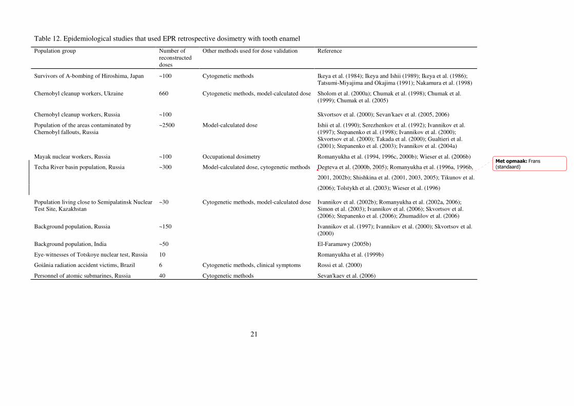
21

Table 12. Epidemiological studies that used EPR retrospective dosimetry with tooth enamel

Population group Number of reconstructed doses

Other methods used for dose validation Reference

Survivors of A-bombing of Hiroshima, Japan ~100 Cytogenetic methods Ikeya et al. (1984); Ikeya and Ishii (1989); Ikeya et al. (1986); Tatsumi-Miyajima and Okajima (1991); Nakamura et al. (1998)

Chernobyl cleanup workers, Ukraine 660

Cytogenetic methods, model-calculated dose Sholom et al. (2000a); Chumak et al. (1998); Chumak et al. (1999); Chumak et al. (2005)

Chernobyl cleanup workers, Russia ~100 Skvortsov et al. (2000); Sevan'kaev et al. (2005, 2006)

Population of the areas contaminated by Chernobyl fallouts, Russia

~2500 Model-calculated dose Ishii et al. (1990); Serezhenkov et al. (1992); Ivannikov et al. (1997); Stepanenko et al. (1998); Ivannikov et al. (2000); Skvortsov et al. (2000); Takada et al. (2000); Gualtieri et al. (2001); Stepanenko et al. (2003); Ivannikov et al. (2004a)

Mayak nuclear workers, Russia ~100 Occupational dosimetry Romanyukha et al. (1994, 1996c, 2000b); Wieser et al. (2006b)

Techa River basin population, Russia ~300 Model-calculated dose, cytogenetic methods Degteva et al. (2000b, 2005); Romanyukha et al. (1996a, 1996b,

2001, 2002b); Shishkina et al. (2001, 2003, 2005); Tikunov et al.

(2006); Tolstykh et al. (2003); Wieser et al. (1996)

Population living close to Semipalatinsk Nuclear Test Site, Kazakhstan

~30 Cytogenetic methods, model-calculated dose Ivannikov et al. (2002b); Romanyukha et al. (2002a, 2006); Simon et al. (2003); Ivannikov et al. (2006); Skvortsov et al. (2006); Stepanenko et al. (2006); Zhumadilov et al. (2006)

Background population, Russia ~150 Ivannikov et al. (1997); Ivannikov et al. (2000); Skvortsov et al. (2000)

Background population, India ~50 El-Faramawy (2005b)

Eye-witnesses of Totskoye nuclear test, Russia 10 Romanyukha et al. (1999b)

Goiânia radiation accident victims, Brazil 6 Cytogenetic methods, clinical symptoms Rossi et al. (2000)

Personnel of atomic submarines, Russia 40 Cytogenetic methods Sevan'kaev et al. (2006)

Met opmaak: Frans(standaard)

Pagina 35: [1] Met opmaak fcallens 29-9-2010 16:53:00

Engels (Groot-Brittannië), Spelling en grammatica controleren


Engels (Groot-Brittannië)















1

References

Abragam, A., Bleaney, B., 1970. Electron Paramagnetic Resonance of Transition Ions. Clarendon Press, Oxford, 911 pp.

Aldrich, J.E., Pass, B., 1986. Dental enamel as an in vivo radiation dosimeter: Separation of the diagnostic X-ray dose from the dose due to natural sources. Radiat. Prot. Dosim. 17, 175-179.

Aldrich, J.E., Pass, B., 1988. Determining radiation exposure from nuclear accidents and atomic tests using dental enamel. Health Phys. 54 (4), 469-471.

Aldrich, J.E., Pass, B., Mailer, C., 1992. Changes in the paramagnetic centres in irradiated and heated enamel studied using electron paramagnetic resonance. Int. J. Radiat. Biol. 61 (3), 433-437.

Amira, S., Vanhaelewyn, G., Callens, F., 2001. X- and Q-band EPR of carbonate derived radicals in calcium apatites synthesized at high temperatures and heated tooth enamel. Phys. Chem. Chem. Phys. 3 (9), 1724-1728.

Anderson, C., 1982. Manual for the Examination of the Bone. CRC Press, Inc., Boca Raton, Florida. 116 pp.

Anspaugh, L.R., Degteva, M.O., Vasilenko, E.K., 2002. Mayak Production Association: Introduction. Radiat. Environ. Biophys. 41, 19–22.

Anspaugh, L.R., Shishkina, E.A., Shved, V.A., Degteva, M.O., Tolstykh, E.I., Napier, B.A., 2003. Comments on paper by Hayes, Haskell and Kenner, Health Phys. 85(5), 622-624.

Aoba, T., Yagi, T., 1982. Crystallographic and structural alterations in the mineral phase of human enamel with carious attack. J. Oral Pathol. 11, 201-209.

Aoba, T., Doi, Y., Yagi, T., Okazaki, M., Takahashi, J., Motiwaki, Y., 1982. Electron spin resonance study of sound and carious enamel. Calcif. Tissue Int. 34, S88-S92.

Aragno, D., Fattibene, P., Onori, S., 2000. Dental radiography: Tooth enamel EPR dose assessment from Rando phantom measurements. Phys. Med. Biol. 45, 2671-2683.

Aragno, D., Fattibene, P., Onori, S., 2001. Mechanically induced EPR signals in tooth enamel. Appl. Radiat. Isot. 55, 375-382.

Atherton, N.M., 1993. Principles of Electron Spin Resonance, Ellis Horwood, Chichester, 585 pp.

Atkins, P.W., Keen, N., Symons, M.C.R., 1962. Oxides and oxyions of the non-metals. Part II. CO2

- and NO2. J. Chem. Soc. 3, 2873-2880.

Atkins, P.W., Symons, M.C.R., 1967. The Structure of Inorganic Radicals. Elsevier, Amsterdam.

Attix, F.H., 1986. Introduction to Radiological Physics and Radiation Dosimetry. Wiley, 607 pp.

Bachmann, C.H., Ellis, E.H., 1965. Fluorescence of bone. Nature 206, 1328-1331.

2

Bachmann, L., Diebolder, R., Hibst, R., Zezell, D.M., 2003. Infrared absorption bands of enamel and dentine tissues from human and bovine teeth. Appl. Spectr. Rev. 38, 1-14.

Bachmann, L., Baffa, O., Gomes, A.S.L., Zezell , D.M., 2004. Chemical origin of the native ESR signals in thermally treated enamel and dentin. Physica B 349, 119–123.

Bacquet, G., Dugas, J., Escribe, C., Youdri, L., Belin, C., 1975. ESR of CO33--Li+

centre in irradiated synthetic single crystal calcite. J. Phys. 36, 427-429.

Bacquet, G., Truong, V.Q., Vignoles, M., Trombe, J.C., Bonel, G., 1981. ESR of CO2-

in x-irradiated tooth enamel and A-type carbonated apatite. Calcif. Tissue Int. 33, 105-109.

Balonov, M., Alexakhin, R., Bouville, A., Liljinzin, J., 2006. Report from the Techa River dosimetry review workshop held on 8–10 December 2003 at the State Research Centre Institute of Biophysics, Moscow, Russia. Health Phys. 90 (2), 97-113.

Baran, N.P., Maksimenko, V.M., Teslenko, V.V., 1998. On the nature of the EPR background signal on tooth enamel. Preprint of the Obninsk conference/private communication.

Baranov, A.E., Guskova, A.K., Nadejina, N.M., Nugis, V.Yu., 1995. Chernobyl experience: Biological indicators of exposure to ionizing radiation. Stem Cells. 13, Suppl 1, 69-77.

Bartoll, J., Stosser, R., Nofz, M., 2000. Generation and conversion of electronic defects in calcium carbonates by UV/Vis light. Appl. Radiat. Isot. 52, 1099-1105.

Becker, R.O., Marino, A.A., 1966. Electron paramagnetic resonance spectra of bone and its major components. Nature 210, 583-588.

Bennett, B., Repacholi, M., Carr, Z. (Eds.), 2006. Health Effects of the Chernobyl Accident and Special Health Care Programmes. Report of the UN Chernobyl Forum Expert Group "Health". World Health Organization, Geneva. ISBN 9241594179.

Bhat, M., 2005. EPR tooth dosimetry as a tool for validation of retrospective doses: An end-user perspective. Appl. Radiat. Isot. 62 (2), 155-161.

BIPM, 1993. BIPM, IEC, IFCC, ISO, IUPAC, IUPAP, OIML, Guide to the Expression of Uncertainty in Measurement, 1st ed., 1993, ISBN 92-67-10188-9. Bureau International des Poids et Mesures, Paris.

Blank, A., Levanon, H., 2000. Filling factor of a paramagnetic sample in a rectangular cavity: Theory and application. Spectrochim. Acta A, 56, 363-371.

Bochvar, I.A., Kleshchenko, E.D., Kushnereva, K.K., Levochkin, F.K., 1997. Sensitivity of human tooth enamel to α-radiation and neutrons. Atom. Energy 83 (5), 845-847.

Bos, A.J.J. (Ed.), 2008. Proceedings of the 15th Solid State Dosimetry (SSD15). Radiat. Meas. 43 (2-6), 131-131.

Bouville, A., Chumak, V.V., Inskip, P.D., Kryuchkov, V., Luckyanov, N., 2006. The Chernobyl accident: Estimation of radiation doses received by the Baltic and Ukrainian cleanup workers. Radiat. Res. 166 (1), 158-167.

3

Boyde, A., Fortelius, M., Lester, K.S., Martin, L.B., 1988. Basis of the structure and development of mammalian enamel as seen by scanning electron microscopy. Sc. Microsc. 2 (3), 1479-1490.

Brady, J.M., Aarestad, N.O., Swartz, H.M., 1968. In vivo dosimetry by electron spin resonance spectroscopy. Health Phys. 15 (1), 43-47.

Bres, E.F., Cherns, D., Vincent, R., Morniroli, J.P., 1993. Space-group determination of human tooth-enamel crystals. Acta Cryst. B49, 56-62.

Brik, A.B., Brik, V.B., 1998. Mechanisms of diffusion in biominerals and bone demineralization at space flights. Mineralog. J. (Ukraine) 20 (5), 46-61.

Brik, A., Radchuk, V., Scherbina, O., Matyash, M., Gaver, O., 1996. Metamorphic modifications and EPR dosimetry in tooth enamel. Appl. Radiat. lsot. 47 (11-12), 1317-1319.

Brik, A.B., Scherbina, O., Haskell, E. H., Sobotovich, E.V., Kalinichenko, A.M., 1997. Heating related changes in the characteristics of paramagnetic centers in tooth enamel using EPR techniques. Mineralog. J. (Ukraine) 19 (4), 3-12.

Brik, A.B., Haskell, E.H., Scherbina, O.I., Brik, V.B., Atamanenko, O.N., 1998. Alignment of CO2

- radicals of tooth enamel with heating. Mineralog. J. (Ukraine) 20 (4), 26-36.

Brik, A., Baraboy, V., Atamanenko, O., Shevchenko, Yu., Brik, V., 2000a. Metabolism in tooth enamel and reliability of retrospective dosimetry. Appl. Radiat. Isot. 52, 1305-1310.

Brik, A., Haskell, E., Brik, V., Scherbina, O., Atamanenko, O., 2000b. Anisotropy effects of EPR signals and mechanisms of mass transfer in tooth enamel and bones. Appl. Radiat. Isot. 52, 1077-1083.

Brik, A.B., Rosenfeld, L.G., Haskell, E.H., Kenner, G.H., Brik, V.B. 2000c. Formation mechanisms and localization places of CO2

- radicals in tooth enamel. Mineralog. J. (Ukraine) 22 (5/6), 57-67.

Brik, A., Kenner, G., Atamanenko, O., Scherbina, O., Kalinichenko, A., Bagnmut, N. 2001a. Formation mechanisms and dynamic characteristics of free radicals of biominerals as deduced from EPR spectroscopy. Mineralog. J. (Ukraine) 23 (4), 44-55.

Brik, A.B., Ulyanchich, N.V., Kenner, G.H., Brik, V.B., Rice, E.E., Kalinichenko, A.M., Bagmut, N.N., 2001b. EPR of the impurity crystal phases in biominerals and their synthetic analogues. Mineralog. J. (Ukraine) 23 (1), 23-37.

Bube, R.H., Photoelectronic Properties of Solids. 1992. Cambridge University Press, Cambridge.

Calderin, L., Stott, M.J., Rubio, A., 2003. Electronic and crystallographic structure of apatites. Phys. Rev. B 67, 134106 (7 p.).

Callens, F., Verbeeck, R., Martens, L., Matthys, P., Boesman, E., 1985. Electron spin resonance absorption of centres with an orthorhombic g-tensor in polycrystalline substances. Phys. Stat. Sol. A 94, 267-274.

4

Callens, F.J., Verbeeck, R.M.H., Matthys, P.F.A., Martens, L.C., Boesman, E.R., 1987. The contribution of CO3

3- and CO2- to the ESR spectrum near g = 2 of powdered human

tooth enamel. Calcif. Tissue Int. 41, 124-129.

Callens, F., Matthys, P., Boesman, E. 1988. ESR of an O3- centre in KCl. J. Phys. C:

Solid State Phys. 21, 3159-3164.

Callens, F., Matthys, P., Boesman, E., 1989a. Paramagnetic resonance spectrum of CO2-

trapped in KCl. J. Phys. Chem. Solids 50 (4), 377-381.

Callens, F.J., Verbeeck, R.M.H., Naessens, D.E., Matthys, P.F.A., Boesman, E.R., 1989b. Effect of carbonate content on the ESR spectrum near g=2 of carbonated calcium apatites synthesized from aqueous media. Calcif. Tissue Int. 44, 114-124.

Callens, F.J., Verbeeck, R.M.H., Naessens, D.E., Matthys, P.F.A., Boesman, E.R., 1991. The effect of carbonate content and drying temperature on the ESR-spectrum near g=2 of carbonated calcium apatites synthesized from aqueous media. Calcif. Tissue 48, 249-259.

Callens, F., Debuyst, R., Dejehet, F., Idrissi, I., Moens, P., 1995a. Location and motion of isotropic paramagnetic centers in monohydrocalcite. Jpn. J. Appl. Phys. 33, 4044-4050.

Callens, F., Moens, P., Verbeeck, R. 1995b. An EPR study of intact and powdered human tooth enamel dried at 400 °C. Calcif. Tissue Int. 56, 543-548.

Callens, F., Vanhaelewyn, G., Matthys, P., Boesman, E. 1998. EPR of carbonate derived radicals: Applications in dosimetry, dating and detection of irradiated food. Appl. Magn. Reson. 14, 235-254.

Callens, F., Vanhaelewyn, G., Matthys, P., 2002. Some recent multi-frequency electron paramagnetic resonance results on systems relevant for dosimetry and dating. Spectrochim. Acta Part A 58, 1321–1328.

Cardis, E., Krjuchkov, V.P., Anspaugh, L., Bouville, A., Chumak, V.V., Drozdovich, V., Gavrilin, Yu, Golovanov, I., Hubert, P., Illychev S.,, Ivanov, V.K., Kesminiene, A., Kurtinaitis, J., Maceika, E., Malakhova, I.V., Mirhaidarov, A.K., Pitkevitch, V.A., Stengrevics, A., Tekkel, M., Tenet, V., Tsykalo, A., 2003. Reconstruction of Doses for Chernobyl Liquidators. Final Performance Report. Unit of Radiation and Cancer International Agency for Research on Cancer. Lyon, France. Grant No: R01CCR015763 – US CDC 20 March 2003.

Cass, J., Kent, R.S., Marshall, S.A., Zager, S.A., 1974. Electron spin resonance absorption spectrum of HCO3

2- molecule-ions in irradiated single-crystal calcite. J. Magn. Reson. 14, 170-181.

CEC (Commission of the European Communities), 1985. The relative tissue-kerma sensitivity of thermoluminescence materials to neutrons. EUR 10105 (Luxembourg: Directorate-General Science, Research and Development).

CEN, 1996. Detection of irradiated food containing bone - Method by ESR spectroscopy. European Committee for Standardisation, EN 1786:1996. http://ec.europa.eu/food/food/biosafety/irradiation.

5

CEN, 2000. Detection of irradiated food containing cellulose by ESR spectroscopy. European Committee for Standardisation, EN 1787:2000. http://ec.europa.eu/food/food/biosafety/irradiation.

CEN, 2001. Detection of irradiated food containing crystalline sugar by ESR spectroscopy. European Committee for Standardisation, EN 13708:2001. http://ec.europa.eu/food/food/biosafety/irradiation.

Cevc, P., Schara, M., Ravnik, C., 1972. Electron paramagnetic resonance study of irradiated tooth enamel. Radiat. Res. 51, 581-589.

Cevc, P., Schara, M., Ravnik, C., Skaleric, U., 1976. Study of the arrangement of

crystallites in γ-irradiated human enamel by electron paramagnetic resonance. J. Dent. Res. 55(4), 691-695.

Cevc, G., Cevc, P., Schara, M., Skaleric, U., 1980. The caries resistance of human teeth is determined by the spatial arrangement of hydroxyapatite microcrystals in the enamel. Nature 286, 425-426.

Chadwick, D., Cardew, G. (Eds.), 1997. Dental Enamel. CIBA Foundation Symposium No. 205. Wiley, Chichester. ISBN 0-471-96872-2.

Chandra, H., Symons, M.C.R., Griffiths, D.R., 1988. Stable perinaphthenyl radicals in flints. Nature 332, 526-527.

Chantry, G.W., Whiffen, D.H., 1962. Electronic absorption spectra of CO2- trapped in

gamma-irradiated crystalline sodium formate. Mol. Phys. 5 (2), 189-194.

Chantry, G.W., Horsfield, A., Morton, J.R., Whiffen, D.H., 1962. The structure, electron resonance and optical spectra of trapped CO3

- and NO3. Mol. Phys. 5, 589-598.

Chow, L.C., Brown, W.E., 1973. Phosphoric acid conditioning of teeth for pit and

fissure sealants. J. Dent. Res. 52, 1158.

Chumak V, Bailiff I, Baran N, Bugai A, Dubovsky S, Fedosov I, Finin V, Haskell E, Hayes R, Ivannikov A, Kenner G, Kirillov V, Khamidova L, Kolesnik S, Liidja G, Likhtarev I, Lippmaa E, Maksimenko V, Meijer A, Minenko V, Pasalskaya L, Past J, Puskar J, Radchuk V, Wieser A, 1996a. The First International Iintercomparison of EPR-Dosimetry with Teeth: First results. Appl Radiat Isot., 47(11-12), 1281-1286.

Chumak, V., Pavlenko, Ju., Sholom, S., 1996b. An approach to the assessment of overall uncertainty of determination of dose using ESR technique. Appl. Radiat. Isot. 47, 1287-1292.

Chumak, V., Likhtarev, I.A., Sholom, S.S., Pasalskaya, L.F., Pavalenko, Y.V., 1997. Retrospective reconstruction of radiation doses of Chernobyl liquidators by electron paramagnetic resonance. Contract Report 97-2. Armed Forces Radiobiology Research Institute, Bethesda (USA).

Chumak, V., Likhtarev, I., Sholom, S., Meckbach, R., Krjuchkov, V., 1998. Chernobyl experience in field of retrospective dosimetry: Reconstruction of doses to the population and liquidators involved in the accident. Radiat. Prot. Dos. 77, 91-95.

6

Chumak, V.V., Sholom, S.V., Pasalskaya, L.F., 1999. Application of high precision EPR dosimetry with teeth for reconstruction of doses to Chernobyl populations. Radiat. Prot. Dosim. 84, 515-520.

Chumak, V.V., Sholom, S.V., Bakhanova, E.V., Pasalskaya, L.F., Musijachenko, A.V., 2005. High precision EPR dosimetry as a reference tool for validation of other techniques. Appl. Radiat. Isot. 62 (2),141-146.

Chumak, V., Ciesielski, B., Sholom, S., Schultka, K., 2006. Lessons of the 3rd International Intercomparison on EPR Dosimetry with Teeth: Similarities and differences of two successful techniques. Radiat. Prot. Dosim. 120 (1–4) 197–201.

Ciesielski, B., Schultka, K., Wolakiewicz, G., 2006. The effect of heating on background and radiation-induced EPR signals in tooth enamel. Spectrochim. Acta Part A 63, 870–874.

Cole, T., Silver, A.H., 1963. Production of hydrogen atoms in teeth by x-irradiation. Nature 200, 700-701.

Convissar, R.A., Goldstein, E.E., 2003. An overview of lasers in dentistry. Gen. Dent. 51 (5), 436-440.

Currie, L.A., 1997. Detection: International update, and some emerging di-lemmas involving calibration, the blank, and multiple detection decisions. Chemom. Intell. Lab. Syst., 37, 151-181.

Currie, L.A., 2004. Detection and quantification limits: Basic concepts, international harmonization, and outstanding ("low-level") issues. Appl. Radiat. Isot. 61 (2-3), 145-149.

D'Errico, F., McKeever, S.W.S. (Eds.), 2006. Proceedings of the 14th International Conference on Solid State Dosimetry (SSD 2004). Radiat. Prot. Dosim. 120 (1-4), 1-6.

De Oliveira, L.M., De Jesus, E.F., Rossi, A.M., Lopes, R.T., Rodrigues, L.N., Barbosa, R.A., 1999. Energy dependence of EPR signal in synthetic and biological hydroxyapatite irradiated with photons. Radiat. Prot. Dosim. 84 (1-4), 511-514.

Degteva, M.O., Kozheurov, V.P., Vorobiova, M.I., 1994. General approach to dose reconstruction in the population exposed as a result of the release of radioactive wastes into the Techa river. Sci. Total. Environ. 14, 49–61.

Degteva, M.O., Kozheurov, V.P., Burmistrov, D.S., Vorobyova, M.I., Valchuk, V.V., Bougrov, N.G., Shishkina, H.A., 1996. An approach to dose reconstruction for the Urals population. Health Phys. 71, 71–76.

Degteva, M.O., Kozheurov, V.P., Tolstykh, E.I., Vorobiova, M.I., Anspaugh, L.R., Napier, B.A., Kovtun, A.N., 2000a. The Techa River dosimetry system: Methods for the reconstruction of internal dose. Health Phys. 79, 24 –35.

Degteva, M.O., Vorobiova, M.I., Kozheurov, V.P., Tolstykh, E.I., Anspaugh, L.R., Napier, B.A., 2000b. Dose reconstruction system for the exposed population living along the Techa River. Health Phys. 78, 542–554.

Degteva, M.O., Shagina, N.B., Tolstykh, E.I., Vorobiova, M.I., Napier, B.A., Anspaugh, L.R., 2002. Studies on the Techa river populations: Dosimetry. Radiat. Environ. Biophys. 41, 41–44.

7

Degteva, M.O., Anspaugh, L.R., Akleyev, A.V., Jacob, P., Ivanov, D.V., Wieser, A., Vorobiova, M.I., Shishkina, E.A., Shved, V.A., Vozilova, A., Bayankin, S.N., Napier, B.A., 2005. Electron paramagnetic resonance and fluorescence in situ hybridization-based investigations of individual doses for persons living at Metlino in the upper reaches of the Techa river. Health Phys. 88 (2), 139-153.

Degteva, M.O., Vorobiova, M.I., Tolstykh, E.I., Shagina, N.B., Shishkina, E.A., Anspaugh, L.R., Napier, B.A., Bougrov, N.G., Shved, V.A., Tokareva, E.E., 2006. Development of an improved dose reconstruction system for the Techa River population affected by the operation of the Mayak Production Association. Radiat. Res. 166 (1), 255-70.

Desrosiers, M.F., 1990. Assessing radiation dose to food. Nature, 345 (6275), 485.

Desrosiers, M.F., 1993. EPR bone dosimetry - A new approach to spectral deconvolution problems. Appl. Radiat. Isot., 44 (1-2), 81-83.

Desrosiers, M.F., Simic, M.G., Eichmiller, F.C., Johnston, A.D., Bowen, R.L., 1989. Mechanically-induced generation of radicals in tooth enamel. Appl. Radiat. Isot. 40 (10-12), 1195-1197.

Desrosiers, M.F., Skinner, A.F., McLaughlin, W.L., Eaton, G.R. (Eds.), 1993. Proceedings of the 3th International Symposium on ESR Dosimetry and Applications. Appl. Radiat. Isot. 44(1-2), 1-472.

Desrosiers, M.F., Skinner, A.F., Regulla, D.F., Nagy, V., McLaughlin, W.L., Eaton, G.R., Eaton, S.S. (Eds.). 1996. Proceedings of the 4th International Symposium on ESR Dosimetry and Applications. Appl. Radiat. Isot. 47(11-12), 1151-1688.

Desrosiers, M.F., Nagy, V.Y., Romanyukha, A.A., 1999. Comment on article by Haskell, Hayes, and Kenner. Health Phys., 77 (4), 470-471.

Desrosiers, M.F., Regulla, D.F., Skinner, A.F., Skovortsov, V., Fill, U.A., Stepanenko, V. (Eds.), 2000. Proceedings of the International Conference on Biodosimetry and 5th International Symposium on ESR Dosimetry and Applications. Appl. Radiat. Isot. 52 (5), 1019-1392.

Desrosiers, M., Schauer, D.A., 2001. Electron paramagnetic resonance (EPR) biodosimetry. Nucl. Instr. Meth. Phys. Res. B 184 (1-2), 219-228.

Deutsch, D., Alayoff, A., 1987. Changes in amino acid composition and protein distribution during development of human deciduous enamel. Growth, 51, 342-354.

DeWald, J.P., 1997. The use of extracted teeth for in vitro bonding studies: A review of infection control considerations. Dent. Mater. 13 (2), 74-81.

Doi, Y., Aoba, T., Okazaki, M., Takahashi, J., Moriwaki Y., 1979. Analysis of paramagnetic centers in x-ray-irradiated enamel, bone, and carbonate-containing hydroxyapatite by electron spin resonance spectroscopy. Calcif. Tissue Int. 28, 107-112.

Doi, Y., Aoba, T., Moriwaki Y., Okazaki, M., Takahashi J., 1980. Orientations of carbonate ions in human tooth enamel studied with use of the CO3

3- radical ions as probes. J. Dent. Res. 59 (9), 1473-1477.

8

Doi, Y., Aoba, T., Okazaki, M., Takahashi J., Moriwaki Y., 1981a. 13C enriched carbonate apatites studied by ESR: Comparison with human tooth enamel apatites. Calcif. Tissue Int. 33, 81-82.

Doi, Y., Aoba, T., Okazaki, M., Takahashi, J., Moriwaki, Y., 1981b. Organic bound chromium in enamel, dentin and bone studied by electron spin resonance. J. Dent. Res., 60 (6), 1053-1056.

Draper, N.R., Smith, H., 1998. Applied Regression Analysis. (3rd ed.). Wiley, New York. 706 pp.

Driessens, F.C.M., Verbeeck, R.M.H., 1990. Biominerals. CRC Press, Boca Raton, 428 pp. ISBN 0-8493-5280-0.

Dubovskii, S.V., Kirillov, V.A., 2000. The individual form of the background signal in EPR dosimetry of tooth enamel. J. Appl. Spectrosc. 67 (5), 878-882.

Dubovsky, S., Kirillov, V., 2001. Reconstruction of individual absorbed doses by tooth enamel on the base of non-linear simulation of their EPR-spectra. Appl. Radiat. Isot. 54 (5), 833-837.

Eaton, S.S., Eaton, G.R., 1992. Quality assurance in EPR. Bull. Magn. Reson. 13, 83-89.

Egersdorfer, S., Wieser, A., Müller, A. 1996. Tooth enamel as a detector mMaterial for retrospective EPR dosimetry. Appl. Radiat. Isot. 47 (11-12), 1299-1303.

El-Faramawy, N.A., 2005a. Comparison of gamma- and UV-light-induced EPR spectra of enamel from deciduous molar teeth. Appl. Radiat. Isot. 62 (2), 191-195.

El-Faramawy, N.A. 2005b. Estimation of radiation levels by EPR measurement of tooth enamel in Indian populations. Appl. Radiat. Isot. 62, 207–211.

El-Faramawy, N., Wieser, A., 2006. The use of deciduous molars in EPR dose reconstruction. Radiat. Environ. Biophys. 44, 273–277.

El-Faramawy, N.A., Rühm, W., 2007. Additional criteria for EPR dosimetry using tooth enamel. Radiat. Res. 167, 244–250.

Elliott, J.C. 1969. Recent progress in the chemistry, crystal chemistry and structure of the apatites. Calcif. Tissue Res. 3, 293-307.

Elliott, J.C., 1994. Structure and chemistry of the apatites and other calcium orthophosphates. Elsevier, Amsterdam, 387 pp. ISBN 0-444-81582-1.

Elliott, J.C., Mackie, P.E., Young, R.A., 1973. Monoclinic hydroxyapatite. Science 180, 1055-1057.

Elliott, J.C., Holcomb, D.W., Young, R.W., 1985. Infrared determination of the degree of substitution of hydroxyl by carbonate ions in human dental enamel. Calcif. Tissue. Int. 37, 372-375.

Fattibene, P., Aragno, D., Onori, S. 1998. Effectiveness of chemical etching for background electron paramagnetic resonance signal reduction in tooth enamel. Health Physics 75 (5), 500-505.

Fattibene, P., Aragno, D., Onori, S., Pressello, M.C., 2000. Thermal induced EPR signals in tooth enamel. Radiat. Meas. 32, 793-798.

9

Fattibene, P., Angelone, M., Pillon, M., De Coste, V., 2003. Tooth enamel dosimetric response to 2.8 MeV neutrons. Nucl. Instrum. Meth. B 201, 480-490.

Fattibene, P., Angelone, M., De Coste, V., Pillon, M., 2004a. Dosimetric response of tooth enamel to 14 MeV neutrons. Radiat. Env. Bioph. 43(2) 85 – 90.

Fattibene, P., Angelone, M., Pillon, M., De Coste, V., 2004b. In phantom dosimetric response of tooth enamel to neutrons. Radiat Prot Dosim 110, 559-563.

Fattibene, P., Carosi, A., De Coste V., Sacchetti, A., Nucara, A., Postorino, P., Dore, P., 2005. A comparative EPR, infrared and Raman study of natural and deproteinated tooth enamel and dentin. Phys. Med. Biol. 50 (6), 1095-1108.

Fattibene, P., Carosi, A., De Coste, V., Onori, S., 2006. EPR properties of intact and deproteinated dentin. Radiat. Prot. Dosim. 120 (1-4), 216-220.

Fawcett, D.W., Jensh, R.P., 2002. Bloom and Fawcett’s Concise Histology. (2nd ed.). Arnold (New York), 360 pp. ISBN 034080677X.

Fincham, A.G., Simmer, J.P., 1997. Amelogenin proteins of developing dental enamel. In: Chadwick, D., Cardew, G. (Eds.), Dental Enamel, CIBA Foundation Symposium No. 205, Wiley, pp. 118-130. ISBN 0-471-96872-2

Fisher, B.V., Morgan, R.E., Phillips, G.O., Wardale, H.W., 1971. Radiation damage in calcium phosphates and collagen: An interpretation of ESR spectra. Radiat. Res. 46, 229-235.

Frisch, M. J., Trucks, G. W., Schlegel, H. B., Scuseria, G. E., Robb, M. A., Cheeseman, J. R., Montgomery, J. A., Jr., Vreven, T., Kudin, K.N., Burant, J. C., Millam, J. M., Iyengar, S. S., Tomasi, J., Barone, V.,Mennucci, B., Cossi, M., Scalmani, G., Rega, N., Petersson, G. A.,Nakatsuji, H., Hada, M., Ehara, M., Toyota, K., Fukuda, R., Hasegawa, J., Ishida, M., Nakajima, T., Honda, Y., Kitao, O., Nakai, H., Klene, M., Li, X., Knox, J. E., Hratchian, H. P., Cross, J. B., Adamo, C., Jaramillo, J., Gomperts, R., Stratmann, R. E., Yazyev, O., Austin, A. J., Cammi, R., Pomelli, C., Ochterski, J. W., Ayala, P. Y., Morokuma, K., Voth, G. A.,Salvador, P., Dannenberg, J. J., Zakrzewski, V. G., Dapprich, S., Daniels, A. D., Strain, M. C., Farkas, O., Malick, D. K., Rabuck, A. D., Raghavachari, K., Foresman, J. B., Ortiz, J. V., Cui, Q., Baboul, A. G., Clifford, S., Cioslowski, J., Stefanov, B. B., Liu, G., Liashenko, A., Piskorz, P., Komaromi, I., Martin, R. L., Fox, D. J., Keith, T., Al-Laham, M. A., Peng, C. Y., Nanayakkara, A., Challacombe, M., Gill, P. M. W., Johnson, B., Chen, W., Wong, M. W., Gonzalez, C., Pople, J. A., 2003, Gaussian 03, Revision B.3, Gaussian, Inc., Pittsburgh, PA.

Galtsev, V.E., 1996. Radiation induced paramagnetic centers in human tooth enamel as studied by ENDOR. Appl. Radiat. Isot. 47 (11/12), 1365-1368.

Galtsev, V.E., Galtseva, E.V., Grinberg, O.Y., Lebedev, Y.S., 1994. Human tooth EPR dosimetry with enhanced sensitivity. J. Radioanal. Nucl. Chem. Letters 186 (1), 35-45.

Galtsev, V.E., Galtseva, E.V., Lebedev, YA.S., 1996. Optimal registration conditions for tooth EPR dosimetry at low accumulated dose. Appl. Radiat. Isot. 47 (11/12), 1311-1315.

Geoffroy, M., Tochon-Danguy, H.J., 1985. Long-lived radicals in irradiated apatites of biological interest: An e.s.r. study of apatite samples treated with 13CO2. Int. J. Radiat. Biol. 48, 621-633.

10

Gerson, F., Huber, W., 2003. Electron spin resonance spectroscopy of organic radicals. Wiley-VCH Weinheim. 464 pp. ISBN 3527302751.

Godfrey-Smith, D.I., Pass, B., 1997. A new method of retrospective radiation dosimetry: Optical stimulated luminescence in dental enamel. Health Phys. 72 (5), 744-749.

Goksu, H.Y., Semiochkina, N., Shiskina, E.A., Wieser, A. El-Faramawy, N.A., Degteva, M.O., Jacob, P. Ivanov, D.V., 2002. Thin layer alpha-Al2O3: C beta dosemeters for the assessment of current dose rate in teeth due to Sr-90 intake, and comparison with electron paramagnetic resonance dosimetry. Radiat. Prot. Dosim. 101 (1-4), 507-513.

Goldman, M., Della Rosa, R.J., 1967. Studies on the dynamics of strontium metabolism under condition of continual ingestion to maturity. Strontium metabolism. In: Lenihan, J.M.A. (Ed.), Proceedings of the International Symposium on Strontium Metabolism. Academic, London, pp. 181–194. LCCN 67-24318.

Goldman, M., Pool, R., Momeni, M. H., Wilson, F., Williams, Chrisp, C., Rosenblatt, L. S., Bustad L. K., 1972. Quantitation of 90Sr toxicity in dogs. In: Proceedings of the Second International Conference on Strontium Metabolism (Glasgow and Strotian, 16-19 August 1972), National Technical Information Service, Springfield (VA), pp. 17-30. OCLC 14435442.

Gordy, W., Aard, W.B., Shields, H., 1955. Microwave spectroscopy of biological substances. In: Paramagnetic resonance in x-irradiated amino acids and proteins. Proc. Natl. Acad. Sci. USA, 41, 983-996.

Griffith, R.V., 1998. Retrospective dosimetry needs from an IAEA perspective. Radiat. Prot. Dosim. 77, 3-9.

Grün, R., 1994. The kinetics of TL peaks and its effect on the dose versus temperature plot. Rad. Meas. 23 (1), 175-194.

Grün, R., 1996. Errors in dose assessment introduced by the use of the "linear part" of a saturating dose response curve. Radiat. Meas. 26 (2), 297-302.

Grün. R., 2006a. Direct dating of human fossils. Yearbook Phys. Anthropol. 49, 2-48.

Grün, R., 2006b. A simple method for the rapid assessment of the qualitative ESR response of fossil samples to laboratory irradiation. Radiat. Meas. 41, 682-689.

Grün, R., Rhodes, E.J., 1991. On the selection of dose points for ESR/TL dose response curves. Ancient TL 9, 40-46.

Grün, R., Rhodes, E.J., 1992. Simulations of saturating exponential ESR/TL dose response curves - weighting of intensity values by inverse variance. Ancient TL 10 (3), 50-56.

Grün, R., Brumby, S., 1994. The assessment of errors in the past radiation doses extrapolated from ESR/TL dose response data. Radiat. Meas. 23, 307-315.

Grün, R., Ward, K., 2002. A long-term fading study for ESR intensity measurement and dose evaluation on fossil tooth enamel. Radiat. Meas. 35, 269 – 274.

Grün, R., Kohno, H., Tani, A., Yamanaka, C., Ikeya, M., Huang, H.P., 1997. Pulsed ESR measurements on fossil teeth. Rad. Meas. 27 (2), 425-431.

11

Grün, R., Joannes-Boyau, R., Stringer, C., 2008. Two types of CO2- radicals threaten the

fundamentals of ESR dating of tooth enamel. Quat. Geo. 3 (1-2), 150-172.

Gualtieri, G., Sgattoni, R., Frascaria, M., Giannoni, M., 1999. Use of electronic spin resonance in the study of dental enamel caries. Preliminary results. Minerva Stomatol. 48 (6), Suppl. 1, 35-41.

Gualtieri, G., Colacicchi, S., Sgattoni, R., Giannoni, M., 2001. The Chernobyl accident: EPR dosimetry on dental enamel of children. Appl. Radiat. Isot. 55, 71–79.

Gusev, B.I., Abylkassimova, Z.N., Apsalikov, K.N., 1997. The Semipalatinsk nuclear test site: a first assessment of the radiological situation and the test-related radiation doses in the surrounding territories. Radiat. Environ. Biophys. 36, 201–204.

Halliday, D., Resnick, R., Walker, J., 2005. Fundamentals of Physics, (7th ed.), Wiley, Hoboken (NJ), 1248 pp.

Halliwell, B., Gutteridge, J., 2007. Free Radicals in Biology and Medicine. Oxford University Press, Oxford, UK, 351 pp.

Hardwick, J.L., 1949. Enamel caries: a chemico-physical hypothesis. Phase one - chemical. Br. Dent. J. 87, 137-142.

Haskell, E.H., Kenner, G.H., Hayes, R.B., 1995. Electron paramagnetic resonance dosimetry of dentine following removal of organic material. Health Phys. 68 (4), 579-584.

Haskell, E.H., Hayes, R.B., Kenner, G.H., 1997a. Improved accuracy of EPR dosimetry using a constant rotation goniometer. Radiat. Meas. 27, 325-329.

Haskell, E.H., Hayes, R.B., Kenner, G.H., Sholom, S.V., Chumak, V.I., 1997b. Electron paramagnetic resonance techniques and space biodosimetry. Radiat. Res. 148, S51-S59.

Hayes, R. H., Haskell, E. H., Romanyukha, A. A., Kenner, G. H., 1998. A technique for increasing reproducibility in EPR dosimetry of tooth enamel. Meas. Sci. Technol. 9, 1994-2006.

Haskell, E. D., Hayes, R. B., Kenner, G. H., 1999a. An EPR dosimetry method for rapid scanning of children following a radiation accident using deciduous teeth. Health Phys. 76, 137-144.

Haskell, E. H., Hayes, R. B., Kenner, G. H., Wieser, A., Aragno, D., Fattibene, P., Onori, S., 1999b. Achievable precision and accuracy in EPR dosimetry of tooth enamel. Radiat. Prot. Dosim. 84, 527-535.

Haskell, E.H., Hayes, R.B., Romanyukha, A.A., Barrus, J.K., Kenner, G.H., 1999c. Automated spectral manipulation and data analysis for EPR dosimetry of teeth. Radiat. Prot. Dosim. 84 (1-4), 521-526.

Hayes, R., 1999. Difficulties with using spectral deconvolution in low-level EPR radiation dosimetry. In: Global ’99, Nuclear Technology, Bridging the Millennia, Proc. of the 5th Int. Conference on Future Nuclear Systems (Jackson Hole, WY, Aug 29 – Sep 3, 1999), American Nuclear Society, La Grange Park, IL, 1999. (A computer optical disk). OCLC 42517684.

Hayes, R., 2003. Diagnostic x ray dose profiles in molar teeth using Monte Carlo simulation. Radiat. Prot. Dosim. 104 (2), 153-158.

12

Hayes, R.B., Haskell, E.H., Kenner, G.H., 1997. A mathematical approach to optimal selection of dose values in the additive dose method of EPR dosimetry. Radiat. Meas. 27 (2), 315-323.

Hayes, R.B., Haskell, E.H., Romanyukha, A.A., Kenner, G.H. 1998a. Technique for increasing reproducibility in EPR dosimetry of tooth enamel. Meas. Sci. Technol. 9, 1994-2006.

Hayes, R. B., Kenner, G. H., Haskell, E. H., 1998b. EPR dosimetry of Pacific walrus (odobenus rosmarus divergens) teeth. Radiat. Prot. Dosim. 77 (1/2), 55–63.

Hayes, R.B., Haskell, E.H., Barrus, J.K., Kenner, G.H., Romanyukha, A.A., 2000a. Accurate EPR radiosensitivity calibration using small sample masses. Nucl. Instrum. Meth. A 441, 535-550.

Hayes, R.B., Haskell, E.H., Kenner, G.H., Barrus, J.K., 2000b. A virtually nondestructive EPR technique accounting for diagnostic X-rays. Radiat. Meas. 32 (5-6), 559-566.

Hayes, R.B., Haskell, E.H., Kenner, G.H., 2002. An EPR model for separating internal Sr-90 doses from external gamma-ray doses in teeth. Health Phys. 83 (1), 75-82.

Holcomb, D.W., Young, R.A., 1980. Thermal decomposition of human tooth enamel. Calcif. Tissue Int. 31, 189-201.

Horowitz, Y.S., Oster, L. (Eds.), 2002. Proceedings of the 13th International Conference on Solid State Dosimetry (SSD 2001), Part II. Radiat. Prot. Dosim. 101 (1-4), 1-612.

Hoshi, M., Toyoda, S., Ivannikov, A., Zhumadilov, K., Fukumura, A., Apsalikov, K., Zhumadilov, Zh. S., Bayankin, S., Chumak, V., Ciesielski, B., De Coste, V., Endo, S., Fattibene, P., Ivanov, D., Mitchell, C. A., Onori, S., Penkowski, M., Pivovarov, S. P., Romanyukha, A., Rukhin, A. B., Schultka, K., Seredavina, T. A., Sholom, S., Skvortsov, V., Stepanenko, V., Tanaka, K., Trompier, F., Wieser, A., Wolakiewicz, G., 2007. Interlaboratory comparison of tooth enamel dosimetry on Semipalatinsk region: Part 1, general view. Radiat. Meas., 42, 1005-1014.

Houben, J.L., 1971. Free radicals produced by ionizing radiation in bone and its constituents. Int. J. Radiat. Biol. 20 (4), 373-389.

Hua, J.P., Callens, F., Cardon, F., De Meyer, H., Vandenbroucke, D., 2000a. Shallow electron traps induced by [Ru(CN)6]

4- in AgCl microcrystals: A computer simulation study of transient microwave photoconductivity. J. Phys. D: Appl. Phys. 33, 564-573.

Hua, J.P., Callens, F., Cardon, F., Vandenbroucke, D., 2000b. Determination of capture cross sections and trap depths of dominant centers in agcl microcrystals doped with [Ru(CN)6]

4- complexes. J. Phys.D: Appl. Phys. 33, 574-583.

Hubbell, J.H., 1982. Photon mass attenuation and energy-absorption coefficients from 1 keV to 20 MeV. Int. J. Appl. Radiat. Isot. 33, 1269-1290.

Hubbell, J.H., Seltzer, S.M., 1995. Tables of x-ray mass attenuation coefficients and mass energy-absorption coefficients 1 keV to 20 MeV for elements Z = 1 to 92 and 48. Additional substances of dosimetric interest. Report NISTIR 5632, National Institute of Standards and Technology, Gaithersburg, MD.

13

IAEA, 1986. Biological Dosimetry: Chromosomal Aberration Analysis for Dose Assessment. Technical Report Series No. 260, International Atomic Energy Agency, Vienna.

IAEA, 2002. Use of the Electron Paramagnetic Resonance Dosimetry with Tooth Enamel for Retrospective Dose Assessment. IAEA-TECDOC-1331, International Atomic Energy Agency, Vienna, Austria, 57 pp.

IARC, 2000. Monographs on the Evaluation of Carcinogenic Risks to Humans. Ionizing radiation, Part 1: X- and Gamma- Radiation, and Neutrons. Vol. 75. International Agency for Research on Cancer. World Health Organization, Geneva.

ICRP, 1991. ICRP Publication 60: 1990 Recommendations of the International Commission on Radiological Protection, Ann. ICRP 21 (1-3), 1-201.

ICRP, 2003a. ICRP Publication 89: Basic Anatomical and Physiological Data for Use in Radiological Protection. International Commission on Radiological Protection. Ann. ICRP 32(3-4), 1-277.

ICRP, 2003b. ICRP Publication 91: A Framework for Assessing the Impact of Ionizing Radiation of Non-Human Species. Ann. ICRP 33, 201-266.

ICRP, 2005. ICRP Publication 96: Protecting People against Radiation Exposure in the Event of a Radiological Attack. Ann. ICRP 35(1), 1-110.

ICRP, 2007. ICRP Publication 103: The 2007 Recommendations of the International Commission on Radiological Protection, Ann. ICRP 37(2-4), 1-332.

ICRU, 1977. Neutron Dosimetry for Biology and Medicine. ICRU Report 26. International Commission on Radiation Units and Measurements, Washington. 128 pp. ISBN 0-913394-20-3.

ICRU, 1989. Tissue Substitutes in Radiation Dosimetry and Measurement, ICRU Report 44. International Commission on Radiation Units and Measurements, Bethesda, MD. 189 pp. ISBN 0-913394-38-6.

ICRU, 1993. Quantities and Units in Radiation Protection Dosimetry. ICRU Report 51.

International Commission on Radiation Units and Measurements, Bethesda, MD. 19 pp. ISBN 0-913394-50-5.

ICRU, 1998. Fundamental Quantities and Units for Ionizing Radiation, ICRU Report 60. International Commission on Radiation Units and Measurements, Bethesda, MD. 23 pp. ISBN 0-913394-59-9.

ICRU, 2002. Retrospective Assessment of Exposures to Ionising Radiations. ICRU Report 68. J. ICRU 2 (2), 144 pp.

Ignatiev, E.A., Lyubashevskii, N.M., Shishkina, E.A., Romanyukha, A.A., 1999. EPR dose reconstruction for bone-seeking Sr-90. Appl. Radiat. Isot. 51 (2), 151-159.

Ignatiev, E.A., Romanyukha, A.A., Koshta, A.A., Wieser, A., 1996. Selective saturation method for EPR dosimetry with tooth enamel. Appl. Radiat. Isot. 47 (3), 333-337.

Ikeya, M., 1993. New Applications of Electron Spin Resonance: Dating, Dosimetry and Microscopy. World Scientific, Singapore. 500 pp. ISBN 9810212003.

14

Ikeya, M., Ishii, H., 1989. Atomic bomb and accident dosimetry with ESR natural rocks and human tooth in vivo spectrometer. Appl. Radiat. Isot. 40 (10-12), 1021-1027.

Ikeya, M., Miyajima, J., Okajima, S., 1984. ESR dosimetry for atomic bomb survivors using shell buttons and tooth enamel. Jpn. J. Appl. Phys. 23, L697-L699.

Ikeya, M., Miki, T., Kai, A., Hoshi, M., 1986. ESR dosimetry of A-bomb radiation using tooth enamel and granite rocks. Radiat. Prot. Dosim. 17, 181-184.

Ikeya, M., Sumitomo, H., Yamanaka, C., Lloyd, D.C., Edwards, A.A., 1996. ESR dosimetry of a deceased radiation worker. Appl. Radiat. Isot. 47 (11-12), 1341-1344.

Ishchenko, S., Vorona, I., Okulov, S., 1999. ENDOR study of irradiated tooth enamel. Semicond. Phys. Quant. Electron. 2 (1), 84-92.

Ishchenko, S.S., Vorona, I.P., Okulov, S.M., Baran, N.P., 2002. 13C hyperfine interactions of CO2

- irradiated tooth enamel as studied by EPR. Appl. Radiat. Isot. 56, 815-819.

Ishii, H., Ikeya, M., 1990. An electron spin-resonance system for in vivo human tooth dosimetry. Jpn. J. Appl. Phys. Part 1. 29, 871-875.

Ishii, H., Ikeya, M., Okano, M., 1990. ESR dosimetry of teeth of residents close to Chernobyl reactor accident. J. Nucl. Sci. Technol. 27 (12), 1153-1155.

ISO, 1984. Dentistry: Designation System for Teeth and Areas of the Oral Cavity. International Organization for Standardization, ISO 3950:1984, ISO, Geneva.

ISO, 1995. Guide to the Expression of Uncertainty in Measurement. ISO/TAG4/WG3. Corrected and Reprinted Edition, 1995. International Organization for Standardization, Geneva. 101 pp. ISBN 9267101889.

ISO, 1996. X and Gamma Reference Radiation for Calibrating Dosemeters and Doserate Meters and for Determining Their Response as a Function of Photon Energy -- Part 1: Radiation Characteristics and Production Methods. International Organization

for Standardization, Geneva, ISO 4037-1. OCLC 39636158.

ISO, 2004. Standard Practice for Use of the Alanine/EPR Dosimetry System. International Organisation of Standards, ISO/ASTM DIS 51607:2004, International Organization for Standardization, Geneva and American Society for Testing and Materials, West Conshohocken (PA).

ISO, 2005. Determination of the detection limit and decision threshold for ionizing

radiation measurements. Part 7: Fundamentals and general applications. International

Organisation of Standards, Geneva. ISO 11929-7:2005.

IUPAC, 1995. Nomenclature in Evaluation of Analytical Methods Including Detection and Quantification Capabilities. IUPAC Recommendations 1995. International Union of Pure and Applied Chemistry. 25 pp.

Ivannikov A.I., Skvortsov, V.G., Stepanenko, V.F., Tikunov, D.D., Fedosov, I.M., Romanyukha, A.A., Wieser, A., 1997. Widescale EPR tooth dosimetry. Results and problems. Radiat. Prot. Dosim. 71, 175-80.

15

Ivannikov, A.I., Skvortsov, V.G., Stepanenko, V.F., Tsyb, A.F., Khamidova, L.G. , Tikunov, D.D., 2000. Tooth enamel EPR dosimetry: Sources of errors and their correction. Appl. Radiat. Isot. 52, 1291-1296.

Ivannikov, A.I, Skvortsov, V.G., Stepanenko, V.F., Tikunov, D.D., Takada, J., Hoshi, M., 2001a. EPR tooth enamel dosimetry: optimization of the automated spectra deconvolution routine. Health Phys. 81 (2), 124-137.

Ivannikov, A.I., Tikunov, D.D., Skvortsov, Stepanenko, V.F., Khomichyonok, V.V., Khamidova, L.G., Skripnik, D.D., Bozadjiev, L.,L., Hoshi, M., 2001b. Elimination of the background signal in tooth enamel samples for EPR-dosimetry by means of physical-chemical treatment. Appl. Radiat. Isot. 55 (5), 701-705.

Ivannikov, A.I., Trompier, F., Gaillard-Lecanu, E., Skvortsov, V.G., Stepanenko, V.F., 2002a. Optimisation of recording conditions for the electron paramagnetic resonance signal used in dental enamel dosimetry. Radiat. Prot. Dosim. 101 (1-4), 531-538.

Ivannikov, A.I., Zhumadilov, Z.H., Gusev, B.I., Miyazawa, C.H., Jiao, L., Skvortsov, V.G., Stepanenko, V.F., Takada, J., Hoshi, M., 2002b. Individual dose reconstruction among residents living in the vicinity of the Semipalatinsk nuclear test site using EPR spectroscopy of tooth enamel. Health Phys. 83 (2), 183-196; and Erratum in Health Phys. 86 (6), 633 (2004).

Ivannikov, A.I., Gaillard-Lecanu, E., Trompier, F., Stepanenko, V.F.; Skvortsov, V.G.; Borysheva, N.B.; Tikunov, D.D., Petin, D.V., 2004a. Dose reconstruction by EPR spectroscopy of tooth enamel: Application to the population of Zaborie village exposed to high radioactive contamination after the Chernobyl accident. Health Phys. 86 (2), 121-134.

Ivannikov, A.I., Tikunov, D.D., Borysheva, N.B., Trompier, F., Skvortsov, V.G., Stepanenko, V.F., Hoshi, M., 2004b. Calibration of EPR signal dose response of tooth enamel to photons: Experiment and Monte Carlo simulation. Radiat. Prot. Dosim. 108, 303-315.

Ivannikov, A., Zhumadilov, K., Tieliewuhan, E., Jiao, L., Zharlyganova, D., Apsalikov, K.N., Berekenova, G., Zhumadilov, Z., Toyoda, S., Miyazawa, C., Skvortsov, V., Stepanenko, V., Endo, S., Tanaka, K., Hoshi, M., 2006. Results of EPR dosimetry for population in the vicinity of the most contaminating radioactive fallout trace after the first nuclear test in the Semipalatinsk test site. J. Radiat. Res. (Tokyo). 47, Suppl. A, A39-A46.

Ivannikov, A., Toyoda, S., Hoshi, M., Zhumadilov, K., Fukumura, A., Apsalikov, K., Zhumadilov, Zh., Bayankin, S., Chumak, V., Ciesielski, B., De Coste, V., Endo, S., Fattibene, P., Ivanov, D., Mitchell, C., Nalapko, M., Onori, S., Penkowski, M., Pivovarov, S., Romanyukha, A., Rukhin, A.B., Schultka, K., Seredavina, T., Sholom, S., Skvortsov, V., Stepanenko, V., Tanaka, K., Trompier, F., Wieser, A., Wolakiewicz, G., 2007. Interlaboratory comparison on tooth enamel dosimetry on Semipalatinsk region: Part 2, effects of spectra processing. Radiat. Meas., 42, 1015-1020.

Iwasaki, M., Miyazawa, C., Uesawa, T. and Niva, K., 1993. Effect of sample grain size on the CO3

3- signal intensity in ESR dosimetry of human tooth enamel. Radioisot. 42, 470–473.

16

Iwasaki, M., Miyazawa, C., Uesawa, T., Itoh, I., Niwa, K., 1995. Differences in the radiation sensitivity of enamel in an individual and among the individuals in dental ESR dosimetry. Radioisot. 44, 785-788.

Iwasaki, M., Miyazawa, C., Chida, T., Takahashi, F., Onai, Y., 2002. Dental ESR dosimetry of a medical physicist who received occupational radiation exposure for almost 40 y. Health Phys. 83 (4), 534-538.

Iwasaki, A., Grinberg, O., Walczak, T., Swartz, H.M., 2005a. In vivo measurements of EPR signals in whole human teeth. Appl Radiat Isot. 62 (2), 187-190.

Iwasaki, A., Walczak, T., Grinberg, O., Swartz, H.M., 2005b. Differentiation of the observed low frequency (1200MHz) EPR signals in whole human teeth. Appl. Radiat. Isot. 62 (2), 133-139.

Jacob, P., Goksu, Y., Taranenko, V., Meckbach, R., Bougrov, N.G., Degteva, M.O., Vorobiova, M.I., 2003. On an evaluation of external dose values in the Techa River Dosimetry System (TRDS) 2000. Radiat. Environ. Biophys. 42, 169 –174.

JCCRER, 1995. Joint Coordination Committee for Radiation Effects Research (JCCRER) Projects in the Russian Health Studies Program. http://www.hss.energy.gov/healthsafety/ihs/ihp/jccrer.html

Jiao, L., Takada, J., Endo, S., Tanaka, K., Zhang, W., Ivannikov, A., Hoshi, M., 2007. Effects of sunlight exposure on the human tooth enamel ESR spectra used for dose reconstruction. J. Radiat. Res. (Tokyo) 48 (1), 21-29.

Johns, H.E., Cunningham, J.R., 1983. The Physics of Radiology. (4th ed.). Charles C. Thomas, Springfield, IL. 796 pp..

Jonas, M., 1995. Spectral deconvolution of the ESR dating signal in fossil tooth enamel. Quatern. Sci. Rev. 14 (4), 431-438.

Jonas, M., 1997. Concepts and methods of ESR dating. Radiat. Meas. 27 (5/6), 943-973.

Jonas, M., Marseglia, E., 1997. A computational model for the simulation of radiation-induced trap-filling in multicrystalline insulators. Rad. Meas. 27 (2), 351-357.

Kellerer, A.M., 2002. The Southern Urals radiation studies. A reappraisal of the current status. Editorial. Radiat. Environ. Biophys. 41, 307–316.

Kenner, G.H., Haskell, E.H., Hayes, R.B., Baig, A., Higuchi, W.I. 1998. EPR properties of synthetic apatites, deorganified dentine and enamel. Calcif. Tissue Int. 62, 443-446.

Kenner, G.H., Brik, A.B., Liu, G., Haskell, E.H., Knight, J.A., Vajda, E.G., Miller, S.C., Jee, W.S.S., Barrus, J.K., 2005. Variation of long-lived free radicals responsible for the EPR native signal of aged or diseased human females and ovariectomized adult rats. Radiat. Meas. 39 (3), 255-262.

Khan R.F.H., Boreham D.R., Rink W.J., 2003a. Quantification of low dose signal in EPR tooth dosimetry - a novel approach. Radiat. Prot. Dosim. 103 (4), 359-362.

Khan, R.F.H., Rink, W.J., Boreham, D.R., 2003b. Biophysical dose measurement using electron paramagnetic resonances in rodent teeth. Appl. Radiat. Isot. 59, 189–196.

17

Khan, R.F.H., Rink, W.J., Boreham, D.R., 2003c. Dosimetric response evaluation of tooth enamel for the accelerator based neutron radiation. Radiat. Meas. 37 (4-5), 355-363.

Khan, R.F.H., Pekar, J., Rink, W.J., Boreham, D.R., 2005. Retrospective radiation dosimetry using electron paramagnetic resonance in canine dental enamel. Appl. Radiat. Isot. 62, 173–179.

Kirillov, V., Dubovsky, S., Tolstik, S., 2002. Artefacts of electron paramagnetic resonance dosimetry caused by a mechanical effect on samples of tooth enamel. Radiat. Prot. Dosim. 102 (1), 41-48.

Kirste, B., 1994. Computational techniques. In: Poole, C.P., Farah, M.A. (Eds.) Handbook of Electron Spin Resonance. AIP Press, Woodbury, NY, 660 pp.

Kittel, C. 1996. Introduction to Solid State Physics. Wiley, New York, 673 pp.

Kleinerman, R.A., Romanyukha, A.A., Schauer, D.A., Tucker, J.D., 2006. Retrospective assessment of radiation exposure using biological dosimetry: Chromosome painting, electron paramagnetic resonance and the glycophorin a mutation assay. Radiat. Res. 166 (1, Pt 2), 287-302.

Knoll, G.F., 1979. Radiation Detection and Measurement. Wiley, New York, 816 pp. ISBN 0-471-49545-X.

Koshta, A.A., Wieser, A., Ignatiev, E.A., Bayankin, S., Romanyukha, A.A., Degteva, M.O., 2000. New computer procedure for routine EPR-dosimetry on tooth enamel. Description and verification. Appl. Radiat. Isot. 52, 1287–1290.

Kudynski, R., Kudynska, J., Buckmaster, H.A., 1994. The decay constant for irradiated human hair using EPR spectroscopy. Appl. Radiat. Isot. 45(6), 645-650.

Kuhar, M., Cevc, P., Schara, M., Funduk, M., 1997. Enhanced permeability of acid-etched or ground dental enamel. J. Prot. Dent. 77 (6), 578-582.

Kuhar, M., Cevc, P., Schara, M., Funduk, N., 1999. In vitro permeability and scanning electron microscopy study of acid-etched and ground enamel surfaces protected with dental adhesive coating. J. Oral Rehabil. 26 (9), 722-730.

Le Geros, R.Z., 1981. Apatites in biological systems. Prog. Crystal Growth Charact. 4, 1-5.

Liidja, G., Past, J., Puskar, J., Lippmaa, E., 1996. Paramagnetic resonance in tooth enamel created by ultra-violet light. Appl. Radiat. Isot. 47, 785-788.

Liidja, G., Wieser, A., 2002. Electron paramagnetic resonance of human tooth enamel at high gamma ray doses. Radiat. Prot. Dos. 101 (1-4), 503-506.

Lund, A., Shiotani M., (Eds.), 2003. EPR of Free Radicals in Solids: Trends in Methods and Applications (Progress in Theoretical Chemistry and Physics). Wiley, New York, 644 pp.

Lunsford, J.H., Jayne, J.P., 1966. Study of CO radicals on magnesium oxide with electron paramagnetic resonance techniques. J. Chem. Phys. 44 (4), 1492-1496.

Marino, A.A., Becker, R.O., 1967. Evidence for direct physical bonding between the collagen fibres and apatite crystals in bone. Nature 213, 697-698.

18

Marsh, R.E., Prestwich, W.V., Rink, W.J., Brennan, B.J., 2002. Monte Carlo determinations of the beta dose rate to tooth enamel. Radiat. Meas. 35 (6), 609-616.

Marshall, S.A., McMillan, J.A., 1968. Electron spin resonance absorption spectrum of Y3+-stabilized CO3

3- molecule-ion in single-crystal calcite. J. Chem. Phys. 48 (11), 5131-5137.

Marshall, S.A., Reinberg, A.R., Serway, R.A., Hodges, J.A., 1964. Electron spin resonance absorption spectrum of CO2

- molecule-ions in single crystal calcite. Mol. Phys. 8, 225-231.

Martens, L.C., Verbeeck, R.M.H., Callens, F.J., Matthys, P.F.A., Driessens, F.C.M., Dermaut, L.R., 1986. The microcrystal alignment in human tooth enamel from carious and non-carious teeth in relation to caries susceptibility. J. Biol. Buccale, 14, 65-68.

Martin, L.B., Boyde, A., Grine, F.E., 1988. Enamel structure in primates: A review of scanning electron microscope studies. Scanning Microsc., 2 (3), 1503-1526.

Mathias, A. (Ed.), 2006. Alanine dosimetry for clinical applications. Physikalisch-Technische Bundesanstalt. PTB-DOS-51. ISBN 3-86509-526-7.

Mazur, M., Valko, M., Morris, H., 2000. Analysis of the radial and longitudinal effect in a double TE104 and a single TE102 rectangular cavity. J. Magn. Reson. 142, 37-56.

McKeever, S. (Ed.), 2000. Proceedings of the 9th International Conference on Luminescence and Electron-Spin Resonance Dating (LED99). Radiat. Meas. 32 (5-6), 385-880.

McMillan, J.A., Marshall, S.A., 1968. Motional effects in the electron spin resonance absorption spectrum of CO2

- molecule-ions in single-crystal calcite. J. Chem. Phys. 48 (1), 467-471.

Meguro, K., Ikeya, M., 1993. Stabilization of superoxide and CO3- radicals through

crystallization of CaCO3. Jpn. J. Appl. Phys. 32, 3540-3543.

Mengeot, M., Harvill, M.L., Gilliam, O.R., 1973. Hydrothermal growth of calcium hydroxyapatite single crystals. J. Cryst. Growth 19, 199-203.

Mengeot, M., Bartram, R.H., Gilliam, O.R., 1974. Paramagnetic holelike defect in irradiated calcium hydroxyapatite single crystals. Phys. Rev. B 11 (11), 4110-4123.

Meriaudeau, P., Vedrine, J.C., Taarit, Y.B., Naccache, C., 1975. Electron paramagnetic resonance studies of CO2

- radicals adsorbed on MgO. J. Chem. Soc. Faraday Trans. II 71, 736-748.

Mineyeva, R.M., Bershov, L.V., Speranskiy A.V., 1993. Electron paramagnetic resonance of Sc3+-stabilized CO3

3- molecule-ion in natural calcite. Phys. Chem. Minerals 20, 136-140.

Mironova-Ulmane, N., Pavlenko, A., Zvagule, T., Karner, T., Bruvere, R., Volrate, A., 2001. Retrospective dosimetry for Latvian workers at Chernobyl. Radiat. Prot. Dosim. 96(1-3), 237-240.

Miyake, M., Liu, K.J., Walczak, T., Swartz, H.M., 2000. In vivo EPR dosimetry of accidental exposures to radiation: Experimental results indicating the feasibility of practical use in human subjects. Appl. Radiat. Isot. 52 (5), 1031–1038.

19

Moens, P., Callens, F., Matthys, P., Maes, F., Verbeeck, R., Naessens, D., 1991. Adsorption of carbonate-derived molecules on the surface of carbonate-containing apatites. J. Chem. Soc. Faraday Trans. 87 (19), 3137-3147.

Moens, P.D.W., Callens, F.J., Verbeeck, R.M.H., Naessens, D.E., 1993a. An EPR spectrum decomposition study of precipitated carbonated apatites (NCAp) dried at 25 °C – Adsorption of molecules from the atmosphere on the apatite powders. Appl. Radiat. Isot. 44 (1-2), 279-285.

Moens, P., De Volder, P., Hoogewijs, R., Callens, F., Verbeeck, R., 1993b. Maximum-likelihood common-factor analysis as a powerful tool in decomposing multicomponent EPR powder spectra. J. Magn. Reson. A 101, 1-15.

Moens, P.D.W., Verbeeck, R.M.H., De Volder, P.J., Callens, F.J., De Maeyer, E.A.P., 1993c. Spectrum decomposition through maximum likelihood common factor analysis of the EPR spectra of Na+ containing carbonated apatites dried at 400 °C. Calcif. Tissue Int. 53, 416-423.

Moens, P.D.W., Callens, F.J., Matthys, P.F.A., Boesman, E.R., Verbeeck, R.M.H., 1994a. EPR study of carbonate derived and ozonide radicals in carbonated apatites synthesized from aqueous solutions. Appl. Magn. Reson. 6, 121-144.

Moens, P.D., Callens, F.J., Matthys, P.F., Verbeeck, R.M., 1994b. 31P and 1H powder endor and molecular orbital study of a CO3

3- ion in x-irradiated carbonate containing hydroxyapatites. J. Chem. Soc. Faraday Trans. 90 (18), 2653-2662.

Moens, P.D., Van Doorslaer S.E., Callens, F.J., Maes, F.R., Matthys, P.F., D’heer, J.M. 1994c. EPR Study of NaCl:CO2

- and NaCl:SO2-. J. Chem. Soc. Faraday Trans. 90 (21),

3261-3265.

Moens, P.D.W., Callens, F.J., Boesman, E.R., Verbeeck, R.M.H., 1995. 1H and 31P ENDOR of the isotropic CO2

- signal at g = 2.0007 in the EPR spectra of precipitated carbonated apatites. Appl. Magn. Reson. 9, 103-113.

Moens, P., Callens, F., Van Doorslaer, S., Matthys, P., 1996. ENDOR study of an O- ion in x-ray-irradiated carbonated hydroxyapatite powders. Phys. Rev. B 53 (9), 5190-5197.

Mombourquette, M.J., Weil J.A., 1992. Simulation of magnetic resonance powder spectra. J. Magn. Reson. 99 (1), 37-44.

Murata, T., Kai, A., Miki, T., 1993. Hydration effects on CO2- radicals in calcium

carbonates and hydroxyapatite. Appl. Radiat. Isot. 44, 305-309.

Murata, T., Shiraishi, K., Ebina, Y., Miki, T., 1996. An ESR study of defects in irradiated hydroxyapatite. Appl. Radiat. Isot. 47 (11/12), 1527-1531.

Nagy, V., 2000. Accuracy considerations in EPR dosimetry. Appl. Radiat. Isot. 52 (5), 1039-1050.

Nagy, V.Y., Placek, J., 1992. Improvement of analytical accuracy of EPR spectrometry by taking into account variation in the shapes of samples. Fresenius J. Anal. Chem. 343, 863-872.

20

Nakamura, N., Miyazawa, C., 1997. Alkaline denaturation of dentin - A simple way to isolate human tooth enamel for electron spin resonance dosimetry. J. Radiat. Res. 38 (3), 173-177.

Nakamura, N., Miyazawa, C., Akiyama, M., Sawada, S., Awa, A.A., 1998a. A close correlation between electron spin resonance (ESR) dosimetry from tooth enamel and cytogenetic dosimetry from lymphocytes of Hiroshima atomic-bomb survivors. Int. J. Radiat. Biol. 73, 619-627.

Nakamura, N., Miyazawa, C., Sawada, S., Akiyama, M., Awa, A.A., 1998b. A close correlation between electron spin resonance (ESR) dosimetry from tooth enamel and cytogenetic dosimetry from lymphocytes of Hiroshima atomic-bomb survivors. Int. J. Radiat. Biol. 73 (6), 619-627.

Nelson, W.H., 2005. Dose-response relationships for radicals trapped in irradiated solids. Radiat. Res. 163, 673-680.

Neter, J., Wasserman, W., Kutner, M.H., 1990. Applied Linear Statistical Models: Regression, Analysis of Variance, and Experimental Designs (3rd ed.). Irwin, Homewood, IL, 1181 pp.

NIEHS-NIH, 2006. Spectra simulating program POWFIT. Available from NIEHS-NIH free of charge, < http://tools.niehs.nih.gov/stdb/esdb.cfm>.

Nilsson, J., Lund, E., Lund, A., 2001. The effects of UV-irradiation on the ESR-dosimetry of tooth enamel. Appl. Radiat. Isot. 54, 131-139.

NRC, 1995. Radiation Dose Reconstruction for Epidemiologic Uses, Committee on an Assessment of CDC Radiation Studies, National Research Council, The National Academies Press, Washington, D.C. Available from http://www.nap.edu/books.

Onori, S., Aragno,. D., Fattibene, P., Petetti, E., Pressello, M.C., 2000. ISS protocol for EPR tooth dosimetry. Radiat. Meas. 32 (5-6), 787-792 (Erratum: Radiat. Meas. 33 (3), 389-389).

Ostrowski, K., Dziedzic-Goclawska, A., Stachowich, W., 1980. Stable radiation-induced paramagnetic entities in tissue mineral and their use in calcified tissue research. In: Pryar. W. (Ed.), Free Radicals in Biology, Vol. 4, Academic, New York, pp. 321-344.

Ovenall, D.W., Whiffen, D.H., 1961. Electron spin resonance and structure of the CO2-

radical ion. Mol. Phys. 4, 135-144.

Pass B., 1997. Collective radiation biodosimetry for dose reconstruction of acute accidental exposures: a review. Environ. Health Perspect., 105 (Suppl 6), 1397-1402.

Pass, B., Aldrich, J.E., 1985. Dental enamel as an in vivo dosimeter. Med. Phys. 12 (3), 305-307.

Pass, B., Aldrich, J. E., 1990. Enamel biopsy and tooth restoration for measurements of radiation exposure from nuclear accidents using ESR. J. Dent. Res. 69, 345.

Pass, B., Shames, A.I., 2000. Signal processing for radiation dosimetry using EPR in dental enamel: Comparison of three methods. Radiat Meas 32 (3), 163-167.

Pass, B., Aldrich, J.E., Scallion, P.L., 1990. An analysis of paramagnetic centers in irradiated dentin using electron spin resonance. Calcif. Tissue Int. 46, 166-168.

21

Pass, B., Baranov, A. E., Kleshchenko, E. D., Aldrich, J. E., Scallion, P., Gale, R.P., 1997. Collective bio-dosimetry as a dosimetric ‘Gold-standard’: A study of three radiation accidents. Health Phys. 72, 389–395.

Pass, B., Wood, R.E., Liu, F.F., McLean, M., Aldrich, J.E., 1998. High radiation doses from radiotherapy measured by electron spin resonance in dental enamel. Radiat. Prot. Dosim. 76 (4), 239-247.

Peckauskas, R.A., Pullman, I., 1978a. Radiogenic free radicals as molecular probes in bone. Calcif. Tissue Res. 25, 37-43.

Peckauskas, R.A., Pullman, I. 1978b. Radiation induced free radicals as molecular probes in synthetic apatites. Calcif. Tiss. Res. 25, 191-195.

Petelin, M., Skaleric, U., Cevc, P., Schara, M., 1999. The permeability of human cementum in vitro measured by electron paramagnetic resonance. Arch. Oral Biol., 44 (3), 259-267.

Pilbrow, J.R., 1990. Transition ion electron paramagnetic resonance. Clarendon Press, Oxford, 717 pp. ISBN 0198552149.

Pilbrow, J.R. 1996. ESR fundamentals. Appl. Radiat. Isot. 47 (11/12), 1465-1470.

Pilbrow, J.R., 1997, Subtleties in electron paramagnetic resonance spectroscopy – implications for dating and dosimetry. Radiat. Meas. 27 (2), 413-417.

Polyakov, V., Haskell, E., Kenner, G., Huett, G., Hayes, R., 1995. Effect of mechanically induced background signal on EPR dosimetry of tooth enamel. Radiat. Meas. 24 (3), 249-254.

Poole, C.P. 1996. Electron Spin Resonance: A Comprehensive Treatise on Experimental Techniques (2nd ed.), Dover, Mineola, NY, 780 pp. ISBN 0486694445.

Priest, N.D., Van De Vyver, F.L., 1990. Trace metals and fluoride in bones and teeth. CRC Press, Boca Raton, FL, 390 pp. ISBN 0849361907.

Proceedings of the Tenth International Congress of the International Radiation Protection Association. May 14–19, 2000, Hiroshima, Japan, P-3a-212. (A computer optical disk). OCLC 45442120.

Punchard, N.A., Kelly, F.J. (Eds.), 1996. Free radicals. A practical approach. Oxford University Press. Oxford. ISBN 0-19-963559-5, 310 pp.

Rae, A.D., 1969. Relationship between the experimental Hamiltonian and the point symmetry of a paramagnetic species in a crystal. J. Chem. Phys. 50 (6), 2672-2655.

Regulla, D.F., 2005. ESR spectrometry: a future-oriented tool for dosimetry and dating. Appl Radiat Isot., 62(2), 117-127.

Regulla, D.F., Scharmann, A., McLaughlin, W.L., Skinner, A.F., Desrosiers, M.F. (Eds.), 1989. Proceedings of the 2nd International Symposium on ESR Dosimetry and Applications. Appl. Radiat. Isot. 40(10-12), 829-1246.

Renz, H., Schaffer, V., Duschner, H., Radlanski, R.J., 1997. Incremental lines in root cementum of human teeth: An approach to their ultrastructural nature by microscopy. Adv. Dent. Res. 11 (4), 472-477.

22

Rey, C., Trombe, J.-C., Dugas, J., 1976. Etude par R.P.E. de l’ion O2- dans quelques

apatites oxygénées. C.R. Acad. Sc. Paris 283C, 277-279.

Riley, P.A., 1997. Melanin. Int. J. Biochem. Cell. Biol. 29 (11), 1235-1239.

Rinard, G.A., Quine, R.W. , Harbridge, J.R. , Song, R., Eaton, G.R., Eaton, S.S., 1999. Frequency dependence of EPR signal-to-noise, J. Magn. Reson. 140, 218–227.

Rist, G.H., Hyde, J.S., 1970. Ligand ENDOR of metal complexes in powders. J. Chem. Phys. 52, 4633-4643.

Romanov, S.A., Vasilenko, E.K., Khokhryakov, V.F., Jacob, P., 2002. Studies on the Mayak nuclear workers: Dosimetry. Radiat. Environ. Biophys. 41, 23–28.

Romanyukha, A.A., Regulla, D.F., 1996. Aspects of retrospective dosimetry. Appl. Radiat. Isot. 47 (11/12), 1293-1297.

Romanuykha, A.A., Regulla, D., Vasilenko, E., Wieser, A., 1994. South Ural nuclear workers – comparison of individual doses from retrospective EPR dosimetry an operational personal monitoring. Appl. Radiat. Isot. 45 (12), 1195-1199.

Romanyukha, A.A., Degteva, M.O., Kozheurov, V.P., Wieser, A., Ignatiev, E.A., Vorobiova, M.I., Jacob, P., 1996a. Pilot study of the population of the Ural Region by EPR tooth dosimetry. Radiat. Environ. Biophys. 35, 305-310.

Romanyukha, A.A., Ignatiev, E.A., Degteva, M.O., Kozheurov, V.P., Wieser, A., Jacob, P., 1996b. Radiation Doses from Ural Region. Nature 381, 199-200.

Romanyukha, A.A., Regulla, D., Vasilenko, E.K., Wieser, A., Drozhko, E.G., Lyzlov, A.F., Koshurnikova, N. A., Shilnikova, N. S., Panfilov, A. P., 1996c. Verification of occupational doses at the first nuclear plant in the former Soviet Union. Appl. Radiat. Isot., 47, 1277-1280.

Romanyukha, A.A., Wieser, A., Regulla, D., 1996d. EPR dosimetry with different biological and synthetic carbonated materials. Radiat. Prot. Dosim. 65 (1-4), 389-392.

Romanyukha, A.A., Hayes, R.B., Haskell, E.H., Kenner, G.H., 1999a. Geographic variations in the EPR spectrum of tooth enamel. Radiat. Prot. Dosim. 84 (1-4), 445-449.

Romanyukha, A.A., Ignatiev, E.A., Ivanov, D.V., Vasilyev, A.G., 1999b. The distance effect on individual exposures evaluated from the Soviet nuclear bomb test at Totskoye test site in 1954. Radiat. Prot. Dosim. 86, 53-58.

Romanyukha, A.A., Desrosiers, M.F., Regulla, D.F., 2000a. Current issues on EPR dose reconstruction in tooth enamel. Appl. Radiat. Isot. 52, 1265-1273.

Romanyukha, A.A., Ignatiev, E.A., Vasilenko, E.K., Drozhko, E.G., Wieser, A., Jacob, P., Kerim-Markus, I.B., Kleschenko, E. D., Nakamura, N., Miyazawa, C., 2000b. EPR dose reconstruction for Russian nuclear workers. Health Phys. 78, 15–20.

Romanyukha, A.A., Nagy, V., Sleptchonok, O., Desrosiers, M.F., Jiang, J., Heis, A. 2000c. Individual biodosimetry at the natural radiation background level. Health Phys, 80 (1), 71-73.

Romanyukha, A. A., Seltzer, S. M., Desrosiers, M., Ignatiev, E. A., Ivanov, D. V., Bayankin, S., Degteva, M. O., Eichmiller, F. C., Wieser, A., Jacob, P., 2001.

23

Correction factors in the EPR dose reconstruction for Techa Riverside residents. Health Physics, 81 (5), 554-566.

Romanyukha, A.A., Desrosiers, M. F., Slepchonok, O. F., Land, C., Luckyanov, N., Gusev, B. I., 2002a. EPR dose reconstruction of two Kazakh villages near the semipalatinsk nuclear test site. Appl. Magn. Reson. 22, 347-356.

Romanyukha, A.A., Mitch, M.G., Lin, Z.C., Nagy, V. and Coursey, B. M., 2002b. Mapping the distribution of Sr-90 in teeth with a photostimulable phosphor imaging detector. Radiat. Res. 157 (3), 341-349.

Romanyukha, A.A., Schauer, D.A., Thomas, J.A., Regulla, D.F. 2005. Parameters affecting EPR dose reconstruction in teeth. Appl. Radiat. Isot. 62, 147-154.

Romanyukha, A.A., Schauer, D.A., Malikov, Y.K., 2006. Analysis of current assessments and perspectives of ESR tooth dosimetry for radiation dose reconstruction of the population residing near the Semipalatinsk nuclear test site. J. Radiat. Res. (Tokyo) 47, Suppl. A, A55-A60.

Romanyukha, A.A., Mitchell, C.A., Schauer, D.A., Romanyukha, L., Swartz, H.M., 2007. Q-band EPR biodosimetry in tooth enamel microsamples: Feasibility test and comparison with X-band. Health Phys. 93 (6), 631-635.

Rossi, A.M., Wafcheck, C.C., de Jesus, E.F., Pelegrini, F., 2000. Electron spin resonance dosimetry of teeth of Goiania radiation accident victims. Appl. Radiat. Isot. 52, 1297-1303.

Roufosse, A., Stapelbroek, M., Bartram, R.H., Gilliam, O.R., 1974. Oxygen-associated holelike centers in calcium chlorapatite. Phys. Rev. B 9 (3), 855-862.

Roufosse, A., Richelle, L.J., Gilliam, O.R., 1976. Electron spin resonance of organic free radicals in dental enamel and other calcified tissues. Arch. Oral. Biol. 21, 227-232.

Sadlo, J., Callens, F., Michalik, J., Stachowicz, W., Matthys, P., Boesman, E., 1998a. Electron-nuclear double resonance of human tooth enamel heated at 400 °C. Calcif. Tissue Int. 63 (5), 409-415.

Sadlo, J., Matthys, P., Vanhaelewyn, G., Callens, F., Michalik, J., Stachowicz, W., 1998b. EPR and ENDOR of radiation-induced CO3

3- radicals in human tooth enamel heated at 400°C. J. Chem. Soc., Faraday Trans. 94, 3275-3278.

Salikhov, I., Hirata, H., Walczak, T., Swartz, H.M., 2003. An improved external loop resonator for in vivo L-band EPR spectroscopy. J. Magn. Reson. 64 (1), 54-59.

Santos, A.B., Rossi, A.M., Baffa, O., 2005. Study of dental enamel and synthetic hydroxyapatite irradiated by EPR at K-band. Appl. Radiat. Isot. 62, 213-217.

Sasaki, T., Goldberg, M., Takuma, S., Garant, P.R., 1990. Cell Biology of Tooth Enamel Formation: Functional Electron Microscopic Monographs, Karger, Basel, 204 pp. ISBN 3805550456.

Sato, K. 1979. Study of an asymmetric ESR signal in x-irradiated human tooth enamel. Calcif. Tissue Int. 29, 95-99.

Schauer, D.A., Seltzer, S.M., Links, J.M., 1993. Exposure-to-absorbed-dose conversion for human adult cortical bone. Appl. Radiat. Isot. 44 (3), 485-489.

24

Schauer, D.A., Desrosiers, M.F., Le, F.G., Seltzer, S.M., Links, J.M., 1994. EPR dosimetry of cortical bone and tooth enamel irradiated with X-rays and gamma-rays - study of energy-dependence. Radiat. Res. 138 (1), 1-8.

Schlick, S., Silver, B.L., Luz, Z., 1971. ESR of 17O-labeled CO2- radical trapped in a

single crystal of sodium formate. J. Chem. Phys. 54 (3), 867-871.

Schonland, D.S., 1965. Molecular Symmetry: An Introduction to Group Theory and Its Uses in Chemistry, Van Nostrand, London, 298 pp. LCCN 65-20161.

Schramm, D.U., Rossi, A.M., 1999. EPR and ENDOR studies on CO- radicals in γ-irradiated synthetic hydroxyapatites. Phys. Chem. Chem. Phys. 1, 2007-2012.

Schramm, D.U., Rossi, A.M., 2000. EPR and ENDOR studies on CO2- radicals in γ-

irradiated B-type carbonated apatites. Phys. Chem. Chem. Phys. 2000 (2), 1339-1343.

Schramm, D.U., Terra, J., Rossi, A.M., Ellis, D.E., 2001. Configuration of CO2- radicals

in in γ-irradiated A-type carbonated apatites: Theory and experimental EPR and ENDOR studies. Phys. Rev. B 63, 024107 (14 pp.).

Schweiger, A., Jeschke, G., 2001. Principles of Pulse Electron Paramagnetic Resonance. Oxford University Press, Oxford, 578 pp. ISBN 0198506341.

Seltzer, S.M., Romanyukha, A.A., Nagy, V., 2001. Monte Carlo calculations of the dose distribution in teeth due to internal exposure from Sr-90: Application to EPR tooth dosimetry. Radiat. Prot. Dosim. 93 (3), 245-260.

Serezhenkov, V., Domracheva, E., Klevezal, G., Kulikov, S., Kuznetsov, S., Mordvintcev, P., Sukhovskaya, L., Schklovsky-Kordi, N.E., Vanin, A.F. 1992. Radiation dosimetry for residents of the Chernobyl region: A Comparison of cytogenetic and electron spin resonance methods. Radiat. Prot. Dosim., 42 (1), 33-36.

Serezhenkov, V.A., Moroz, I.A., Klevezal, G.A., Vanin, A.F., 1996. Estimation of accumulated dose of radiation by the method of ESR-spectrometry of dental enamel of mammals. Appl. Radiat. Isot. 47 (11/12), 1321-1328.

Serway, R.A., Marshall, S.A., 1967a. Electron spin resonance spectra of CO3- and CO3

3- molecule-ions in irradiated single-crystal calcite. J. Chem. Phys. 46 (5), 1949-1952.

Serway, R.A., Marshall, S.A. 1967b. Electron spin resonance absorption spectrum of orthorhombic CO3

- molecule-ions in irradiated single crystal calcite. J. Chem. Phys. 47, 868-869.

Sevan'kaev A.V., Lloyd D.C., Edwards A.A., Khvostunov I.K., Mikhailova G.F., Golub E.V., Shepel N.N., Nadejina N.M., Galstian I.A., Nugis V.Y., Barrios L., Caballin M.R., Barquinero J.F., 2005. A cytogenetic follow-up of some highly irradiated victims of the Chernobyl accident. Radiat. Prot. Dosim. 113 (2), 152-161.

Sevan'kaev, A., Khvostunov, I., Lloyd, D., Voisin, P., Golub, E., Nadejina, N., Nugis, V., Sidorov, O., Skvortsov, V., 2006. The suitability of FISH chromosome painting and ESR-spectroscopy of tooth enamel assays for retrospective dose reconstruction. J. Radiat. Res. (Tokyo). 47, Suppl. A, A75-A80.

Shaw, W.J., Campbell, A.A., Paine, M.L., Snead, M.L., 2004. The COOH terminus of the amelogenin, LRAP, is oriented next to the hydroxyapatite surface. J. Biol. Chem. 279 (39), 40263-40266.

25

Shimano, T., Iwasaki, M., Miyazawa, C., Miki, T., Kai, A., Ikeya, M., 1989. Human tooth dosimetry for gamma-rays and dental x-rays using ESR. Appl. Radiat. Isot. 40 (10-12), 1035-1038.

Shiraishi, K., Iwasaki, M., Miyazawa, C.,Yonehara, H., Matsumoto, M., 2002. Dose estimation by ESR on tooth enamel from two workers exposed to radiation due to the JCO accident. Radiat. Res. 43, 331–335.

Shishkina, E.A., Lyubashevskii, N.M., Tolstykh, E.I., Ignatiev, E.A., Betenekova, T.A., Nikiforov, S.V., 2001a. A mathematical model for calculation of Sr-90 absorbed dose in dental tissues: Elaboration and comparison to EPR measurements. Appl. Radiat. Isot. 55 (3), 363-374.

Shishkina, E.A., Shved, V.A., Degteva, M.O., Tolstykh, E.I., Ivanov, D.V., Bayankin, S.N., Anspaugh, L.R., Napier, B.A., Wieser, A., Jacob, P., 2001b. Description of the computer database “tooth” and discussion of requirements for EPR measurements to support a validation study of external doses calculated by use of the Techa River Dosimetry System–2000. Urals Research Center for Radiation Medicine and University of Utah; Chelyabinsk and Salt Lake City. Final Report for Milestone 2, Project 1.1. Office of Health Studies, U.S. Dept. of Energy. 60 pp.

Shishkina, E.A., Shved, V.A., Tolstykh, E.I., Degteva, M.O., Anspaugh, L.R., Nagy, V., Mitch, M., 2002. Investigation of the tooth as a complex dosimeter: Formation of dose in tooth enamel. Report for Milestone 2, Project 1.1. Office of Health Studies, U.S. Dept. of Energy. 59 pp.

Shishkina, E.A. , Shved, V.A. , Degteva, M.O. , Tolstykh, E.I. , Ivanov, D.V., Bayankin, S.N., Wieser, A., Göksu, H.Y., El-Faramawy, N.A. , Semiochkina, N., Jacob, P. , Anspaugh, L.R., Napier, B.A., 2003. Issues in the validation of external dose: Background and internal dose components of cumulative dose estimated using the electron paramagnetic resonance (EPR) method. Final Report for Milestone 7, Part 1. US-Russian Joint Coordinating Committee on Radiation Effects Research. Project 1.1., 67 pp.

Shishkina, E.A., Goksu, H.Y., El-Faramawy, N.A., Semiochkina, N., 2005. Assessment of 90Sr concentration in dental tissue using thin-layer beta-particle detectors and verification with numerical calculations. Radiat. Res. 163(4), 462-467.

Sholom, S.V., Chumak, V.V., 2003. Decomposition of spectra in EPR dosimetry using the matrix method. Radiat. Meas. 37 (4-5), 365-370.

Sholom, S.V., Chumak, V.V., 2005. Variability of parameters in retrospective EPR dosimetry with teeth for Ukrainian population. Appl. Radiat. Isot. 62 (2), 201-206.

Sholom, S., Chumak, V. and Pavlenko, J., 1997. The doses from diagnostic x-ray procedures in the EPR-spectroscopy technique with tooth enamel. In: Proc. IRPA Regional Symposium on Radiation Protection in Neighboring Countries of Central Europe, 8–12 September 1997, Prague. pp. 571–574. OCLC 441626082.

Sholom, S.V., Haskell, E.H., Hayes, R.B., Chumak, V.V., Kenner, G.H., 1998a. Influence of crushing and additive irradiation procedure on EPR dosimetry of tooth enamel. Radiat. Meas. 29 (1), 105-111.

26

Sholom, S.V., Haskell, E.H., Hayes, R.B., Chumak, V.V.,Kenner, G.H., 1998b. Properties of light induced EPR signals in enamel and their possible interference with gamma-induced signals. Radiat. Meas. 29, 113-118.

Sholom S.V., Chumak V.V., Pasalskaja L.F., 2000a. Some aspects of EPR dosimetry of liquidators. Appl. Radiat. Isot. 52 (5), 1283-1286.

Sholom, S.V., Haskell, E.H., Hayes, R.B., Chumak, V.V., Kenner, G.H., 2000b. EPR-dosimetry with carious teeth. Radiat. Meas. 32, 799-803.

Sholom, S., Chumak, V., Desrosiers, M., Bouville, A., 2006. A transferability study of the EPR-tooth-dosimetry technique. Radiat. Prot. Dosim. 120 (1–4), 210–215.

Shved, V.A., Shishkina, E.A., 2000. Assessment of tooth tissues dose rate coefficients from incorporated Strontium-90 in EPR dose reconstruction for the Techa riverside population. In: Proceedings of the Tenth International Congress of the International Radiation Protection Association. May 14–19, Hiroshima, Japan, P-3a-212.

Simon, S.L., Baverstock, K.F., Lindholm, C., 2003. A summary of evidence on radiation exposures received near to the Semipalatinsk nuclear weapons test site in Kazakhstan. Health Phys. 84 (6), 718-725.

Simon, S.L., Beck, H.L., Gordeev, K., Bouville, A., Anspaugh, L.R., Land, C.E., Luckyanov, N., Shinkarev, S., 2006a. External dose estimates for Dolon village: Application of the U.S./Russian joint methodology. J. Radiat. Res. (Tokyo). 47, Suppl. A, A143-A147.

Simon, S.L., Kleinerman, R.A., Ron, E., Bouville, A., 2006b. Uses of dosimetry in radiation epidemiology. Radiat. Res. 166(1), 125-127 (and the rest of the issue).

Skaleric, U., Ravnik, C., Cevc, P., Schara, M., 1982. Microcrystal arrangement in human deciduous dental enamel studied by electron paramagnetic resonance. Caries Res. 16, 47-50.

Skinner, A.R., Blackwell, B.A., Chasteen, N.D., Shao, J., Min, S.S., 2000. Improvements in dating tooth enamel by ESR. Appl. Radiat. Isot. 52(5), 1337-1344.

Skinner, A.R., Dennis Chasteen, N., Shao J.L., Blackwell, B.A.B., 2001. Q-band studies of the ESR signal in tooth enamel. Quat. Sci. Rev. 20 (5-9), 1027-1030.

Skinner, A., Fill, U., Baffa, O., Eaton, S. (Eds.), 2005. Proceedings of the 6th International Symposium on ESR Dosimetry and Applications. Appl. Radiat. Isot. 62 (2), 115-382.

Skinner, A., Blakely, W.F., (Eds.), 2007. Proceedings of the 7th International Symposium on ESR Dosimetry and Applications and the 2nd International Conference on Biodosimetry. Radiat.Meas. 42 (6-7), 945-1264.

Skvortzov, V. G., Ivannikov, A. I., Eichhoff, U., 1995. Assessment of individual accumulated irradiation doses using EPR spectroscopy of tooth enamel. J. Mol. Struct. 347, 321-330.

Skvortsov, V.G., Ivannikov, A.I., Stepanenko, V.F., Tsyb, A.F., Khamidova, L.G., Kondrashov, A.E., Tikunov, D.D., 2000. Application of EPR retrospective dosimetry for large-scale accidental situation. Appl. Radiat. Isot. 52, 1275-1282.

27

Skvortsov, V., Ivannikov, A., Tikunov, D., Stepanenko, V., Borysheva, N., Orlenko, S., Nalapko, M., Hoshi, M., 2006. Considerations regarding the implementation of EPR dosimetry for the population in the vicinity of Semipalatinsk nuclear test site based on experience from other radiation accidents. J. Radiat. Res. (Tokyo). 47, Suppl. A, A61-A69.

Sleptchonok, O.F., Nagy, V., Desrosiers, M.F., 2000. Advancements in accuracy of the alanine dosimetry system. Part 1. The effects of environmental humidity. Radiat. Phys. Chem. 57 (2), 115-133.

Sobel, A.E., 1962. Dietary phosphate and caries susceptibility. Dent. Prog. 2, 48-52.

SOUL, 2005. Southern Urals Radiation Risk Research. EURATOM, http://www.gsf.de/soul

Spaeth, J.-M., Niklas, J.R., Bartram, R.H., 1992. Structural Analysis of Point Defects in Solids, Springer, Berlin. 367 pp.

Spaeth, J.-M., Overhof, H., 2003. Point defects in Semiconductors and Insulators, Springer, Berlin. 490 pp.

Stepanenko, V., Skvortsov, V., Tsyb, A., Ivannikov, A., Kondrashov, A., Tikunov, D., Iaskova, E., Shakhtarin, V., Petin, D., Parshkov, E., Chernichenko, L., Snykov, V., Orlov, M., Gavrihn, Yu., Khrousch, V., Shinkarev, S., 1998. Thyroid and whole-body dose reconstruction in Russia following the Chernobyl accident: Review of progress and results. Radiat. Prot. Dosim 77, 101-106.

Stepanenko, V.F., Orlov, M.Y., Petin, D.V., Tikunov, D.D., Borysheva, N.B., Ivannikov, A.I., Skvortsov, V.G., Yas'kova, E.K., Kolyzhenkov, T.V., Kryukova, I.G., Moskovko, L.I., Tsyb, A.F., Proshin, A.B., Rivkind, N.B., 2003. Retrospective individual dosimetry at a populated point with a high degree of radioactive contamination. Atom. Energ. 95 (1), 503-509.

Stepanenko, V.F., Hoshi, M., Bailiff, I.K., Ivannikov, A.I., Toyoda, S., Yamamoto, M., Simon, S.L., Matsuo, M., Kawano, N., Zhumadilov, Z., Sasaki, M.S., Rosenson, R.I., Apsalikov, K.N., 2006. Around Semipalatinsk nuclear test site: Progress of dose estimations relevant to the consequences of nuclear tests (A summary of 3rd Dosimetry Workshop on the Semipalatinsk nuclear test site area, RIRBM, Hiroshima University, Hiroshima, 9-11 March, 2005). J. Radiat. Res. (Tokyo). 47, Suppl. A. A1-A13 (and the rest of the issue).

Stone, A.J. 1963. Gauge invariance of the g tensor. Proc. Roy. Soc. A 271, 424-434.

Stott, G.G., Sis, R.F., Levy, B.M., 1982. Cemental annulation as an age criterion in forensic dentistry. J. Dent. Res. 61, 814-817.

Straume, T., Anspaugh, L.R., Haskell, E.H., Lucas, J.N., Marchetti, A.A., Likhtarev, I.A., Chumak, V.V., Romanyukha, A.A., Khrouch, V.T., Gavrilin, Yu.I., Minenko, V.F., 1997. Emerging technological bases for retrospective dosimetry. Stem Cells. 15, Supplement 2, 183-193.

Suga, S., Watabe, N. (Eds), 1992. Hard Tissue Mineralization and Demineralization. Springer, Tokyo. 197 pp. ISBN 4431700927.

Swartz, H.M., Bolton, J.R., Borg, D.C. (Eds.), 1972. Biological applications of electron spin resonance. Wiley, New York, 569 pp. ISBN 0-471-83870-5.

28

Swartz, H.M., Iwasaki, A., Walczak, T., Demidenko, E., Salikhov, I.,, Lesniewski, P., Starewicz, P., Schauer, D., Romanyukha, A., 2005. Measurements of clinically significant doses of ionizing radiation using non-invasive in vivo EPR spectroscopy of teeth in situ. Appl. Radiat. Isot. 62 (2), 293-299.

Swartz, H.M., Iwasaki, A., Walczak, T., Demidenko, E., Salikhov, I., Khan, N., Lesniewski, P., Thomas, J., Romanyukha, A., Schauer, D., Starewicz, P., 2006. In vivo EPR dosimetry to quantify exposures to clinically significant doses of ionising radiation. Radiat. Prot. Dosim. 120 (1-4),163-170.

Takada, J., Hoshi, M., Endo, S., Stepanenko, V.F., Kondrashov, A.E., Petin, D., Skvortsov, V., Ivannikov, A., Tikounov, D., Gavrilin, Y., Snykov, V.P., 2000. Dosimetry studies in Zaborie village. Appl. Radiat. Isot. 52 (5), 1165-1169.

Takahashi, F., Yamaguchi, Y., Iwasaki, M., Miyazawa, C., Hamada, T., 2001. Relations between tooth enamel dose and organ doses for electron spin resonance dosimetry against external photon exposure. Radiat. Prot. Dosim. 95 (2), 101-108.

Takahashi, F., Yamaguchi, Y., Iwasaki, M., Miyazawa, C., Hamada, T., Funabiki, J., Saito, K., 2002. Conversion from tooth enamel dose to organ doses for electron spin resonance dosimetry. J. Nucl. Sci. Technol. 39 (9), 964-971.

Takahashi, F., Yamaguchi, Y., Iwasaki, M., Miyazawa, C., Hamada, T., Funabiki, J., Saito, K., 2003. Analyses of absorbed dose to tooth enamel against external photon exposure. Radiat. Prot. Dosim. 103 (2), 125-130.

Takano, Y., 1995. Enamel mineralization and the role of ameloblasts in calcium transport. Connect. Tissue Res., 33 (1-3), 127-137.

Tanaka, K., Endo, S., Ivannikov, A., Toyoda, S., Tieliewuhan, E., Zhumadilov, K., Miyazawa, C., Suga, S., Kitagawa K., Hoshi M., 2006. Study on influence of X-ray baggage scan on ESR dosimetry for SNTS using human tooth enamel. J. Radiat. Res. (Tokyo) 47, Suppl. A, A81-A83.

Tani, T. 1995. Photographic Sensitivity, Oxford University Press, Oxford, Ch. 4.

Tatsumi, J., 1986. Dose estimation of radiation-exposed people by ESR. Filmbadge News (Tokyo) 125, 1-10 (in Japanese).

Tatsumi-Miyajima, J., 1987. ESR dosimetry for atomic bomb survivors and radiologic technologists. Nucl. Instrum. Meth. A257, 417-422.

Tatsumi-Miyajima, J., Okajima, S., 1991. Physical dosimetry at Nagasaki - Europium-152 of stone embankment and electron spin resonance of teeth from atomic bomb survivors. J. Radiat. Res. (Tokyo), Suppl., 83-98.

Termine, J.D., Posner, A.S., 1967. Amorphous/crystalline interrelationships in bone mineral. Calcif. Tissue Res. 1, 8-23.

Termine, J.D., Pullman, I., Posner, A.S., 1967. Electron spin resonance study of irradiated bone and its constituents Arch. Biochem. Biophys. 122, 318-330.

Termine, J.D., Eanes, E.D., Greenfield, D.J., Nylen, M.U., Harper, R.A., 1973. Hydrazine deproteinated bone mineral. Physical and chemical properties. Calcif. Tissue Res. 12, 73-90.

29

Thomson, G.H., 1951. The Factorial Analysis of Human Ability (5th ed.). University of London Press, London. 383 pp. OCLC 15613681.

Thorne, M.C., 2003. Background radiation: Natural and man-made. J. Radiol. Prot. 23, 29–42.

Tieliewuhan, E., Ivannikov, A., Zhumadilov, K., Nalapko, M., Tikunov,D., Skvortsov, V., Stepanenko, V., Toyoda, S., Tanaka, K., Endo, S, Hoshi, M., 2006. Spectra processing at tooth enamel dosimetry: Analytical description of EPR spectrum at different microwave power. Radiat. Meas. 41, 410–417.

Tikunov, D., Trompier, F., Ivannikov, A., Clairand, I., Herve, M.L., Khailov, A., Skvortsov, V., 2005. Relative sensitivity of tooth enamel to fission neutrons: Effect of secondary protons. Radiat. Meas. (5), 509-514.

Tikunov, D.D., Ivannikov, A.I., Shishkina, E.A., Petin, D.V., Borysheva, N.B., Orlenko, S., Nalapko, M., Shved, V.A. , Skvortsov, V.G. , Stepanenko, V.F., 2006. Complex experimental research on internal tooth dosimetry for the Techa River region: A model for 90Sr accumulation in human teeth formed by time of intakes. Radiat. Meas. 41, 565 – 576.

Tochon-Danguy, H.J., Very, J.M., Geoffroy, M., Baud, C.A. 1978. Paramagnetic and crystallographic effects of low-temperature ashing on human bone and tooth enamel. Calcif. Tiss. Res. 25, 99-104.

Tolstykh, E. I., Degteva, M. O., Kozheurov, V. P., Shishkina, E. A., Romanyukha, A. A., Wieser, A., Jacob, P., 2000. Strontium metabolism in teeth, and enamel dose assessment: Analysis of the Techa River data. Radiat. Environ. Biophys. 39, 161–171.

Tolstykh, E.I., Shishkina, E.A., Degteva, M.O., Ivanov, D.A., Shved, V.A., Bayankin, S.N., Anspaugh, L.R., Napier, B.A., Wieser, A., Jacob.,P., 2003. Age dependencies of Sr-90 incorporation in dental tissues: Comparative analysis and interpretation of different kinds of measurements obtained for residents on the Techa River. Health Phys. 85 (4), 409-419.

Toyoda, S., Sumitomo, H., Ikeya, M., Ishii, H., 1994. Separation of CO2- signal from a

spectrum of irradiated tooth enamel in ESR dosimetry. In: Uchiyama, M.; Kurotaki, K., Kobayashi, S. (Eds.). Assessment of the Health and Environmental Impact from Radiation Doses due to Released Radionuclides: Proceedings of the International Workshop at Chiba, Jan. 18-20, 1994, National Institute of Radiological Sciences, Chiba, NIRS-M-102. LCCN 95-232635.

Toyoda S, Tanizawa H, Romanyukha AA, Miyazawa C, Hoshi M, Ueda Y, Nitta Y, 2003. Gamma-ray dose response of ESR signals in tooth enamel of cows and mice in comparison with human teeth. Radiat. Meas. 37 (4-5), 341-346.

Toyoda, S., Imata, H., Romanyukha, A.A., Hoshi, M., 2006. Towards high sensititivity ESR dosimetry of mammal teeth: The effct of chemical treatment. J. Radiat. Res. 47, A71-A74.

Trompier, F., Fattibene, P., Tikunov, D., Bartolotta, A., Carosi, A., Doca, M.C., 2004. EPR dosimetry in a mixed neutron and gamma radiation field. Radiat. Prot. Dosim. 110, 437-442.

30

Trompier, F., Tikunov, D. D., Ivannikov, A., Clairand, I. 2006. ESR investigation of joint use of dentin and tooth enamel to estimate photon and neutron dose components of a mixed field. Radiat. Prot. Dosim.120 (1–4), 191–196.

Ulanovsky, A., Wieser, A., Zankl, M., Jacob, P., 2005. Photon dose conversion coefficients for human teeth in standard irradiation geometries. Health Phys, 89 (6), 645–659.

UNSCEAR, United Nations Scientific Committee on the Effects of Atomic Radiation, 2000a. Sources and Effects of Ionizing Radiation. Report of the United Nations Scientific Committee on the Effects of Atomic Radiation to the General Assembly. UNSCEAR 2000 Report. Vol. 1. p. 17.

UNSCEAR, United Nations Scientific Committee on the Effects of Atomic Radiation, 2000b. Sources and effects of ionizing radiation. Vol. 1. Annex B. Exposures from natural radiation sources. UNSCEAR 2000 Report. Vol. 1. p. 74

Van Doorslaer, S., Moens, P., Callens, F., Matthys, P., Verbeeck, R. 1996. 31P and 1H powder ENDOR study of ozonide radicals in carbonated apatites synthesized from aqueous solutions. Appl. Magn. Reson. 10, 87-102.

Van Willigen, H., Roufosse, A.H., Glimcher, M.J. 1980. Proton and phosphorous ENDOR on paramagnetic centers in x-irradiated, oriented human tooth enamel. Calcif. Tissue Int. 31, 70-70.

Vanhaelewyn, G., Callens, F., Grün, R., 2000a. EPR spectrum deconvolution and dose assessment of fossil tooth enamel using maximum likelihood common factor analysis. Appl. Radiat. Isot. 52, 1317-1326.

Vanhaelewyn, G.C.A.M., Morent, R.A., Callens, F.J., Matthys P.F.A.E., 2000b. X- and Q-band electron paramagnetic resonance of CO2

- in hydroxyapatite single crystals. Radiat. Res. 154 (4), 467-471.

Vanhaelewyn, G., Amira, S., Debuyst, R., Callens, F. Glorieux, Th., Leloupc, G., Thierens, H., 2001. A critical discussion of the 2nd Intercomparison on Electron Paramagnetic Resonance Dosimetry with Tooth Enamel. Radiat. Meas. 33, 417–426.

Vanhaelewyn, G., Goovaerts, E., Callens, F., 2002a. Multi-frequency EPR study of radiation-induced radicals in tooth enamel. Radiat. Eff. Defects S. 157 (6-12), 1127-1131.

Vanhaelewyn, G.C.A.M., Sadlo, J., Matthys P.F.A.E., Callens, F.J., 2002b. Comparative X- and Q-band EPR study of radiation-induced radicals in tooth enamel. Radiat. Res. 158 (5), 615-625.

Vanhavere, F., Loos, M., Callens, F., Debuyst, R., de Boer, E., Klaassen, A., 1997. A local intercomparison study of ESR dosimetry using tooth enamel. J. Radioanal. Nuclear Chem. 221 (1-2), 123-126.

Veronese, I., El-Faramawy, N., Giussani, A., Cantone, M.C., Shishkina, E.A., Goksu, H.Y., 2006. The use of alpha-Al2O3:C in Riso OSL single grains attachment system for assessing the spatial dose rate distribution due to incorporation of 90Sr in human teeth. Radiat. Prot. Dosim. 119 (1-4), 408-412.

Vorobiev, A.I., 1997. Acute radiation disease and biological dosimetry in 1993. Stem Cells. 15, Suppl. 2, 269-274.

31

Vorobiova, M.I., Degteva, M.O., Kozyrev, A.V., Anspaugh, L.R., Napier, B.A., 1999. External doses evaluated on the basis of the Techa River dosimetry system approach. US-Russian Joint Coordinating Committee on Radiation Effects Research Project 1.1. “Development of an Improved Dose Reconstruction System for the General Population Affected by the Operation of the Mayak Production Association”. Final Report for Milestone 6. Project 1.1. May 1999. 69 pp.

Vorona, I.P., Ishchenko, S.S., Baran, N.P., 2005. The effect of thermal treatment on radiation-induced EPR signals in tooth enamel. Rad. Meas. 39, 137-141.

Vorona, I.P., Ishchenko, S.S., Baran, N.P., Petrenko, T.L., Rudko, V.V., 2006. Evidence of annealing-induced transformation of CO2

- radicals in irradiated tooth enamel. Radiat. Meas. 41, 577-581.

Vorona, I.P., Baran, N.P., Ishchenko, S.S., Rudko, V.V., 2007. Separation of the contributions from gamma- and UV-radiation to the EPR spectra of tooth enamel plates. Appl. Radiat. Isot. 65 (5), 553-556.

Vugman, N.V., Rossi, A.M., Rigby, S.E., 1995. EPR dating CO2- sites in tooth enamel

apatites by ENDOR and triple resonance. Appl. Radiat. Isot., 46(5), 311-315.

Weil, J.A., Bolton, J.R., Wertz, J.E., 1994. Electron Paramagnetic Resonance: Elementary Theory and Practical Applications. Wiley, New York, 568 pp.

Weise, K., Hübel, K., Rose, E., Schläger, M., Schrammel, D., Täschner, M., Michel, R, 2006. Bayesian decision threshold, detection limit and confidence limits in ionising-radiation measurement. Radiat. Prot. Dosim. 121 (1), 52–63.

Wieser, A., El-Faramawy, N., 2002. Dose reconstruction with electron paramagnetic resonance spectroscopy of deciduous teeth. Radiat. Prot. Dosim. 101 (1–4), 545–548.

Wieser, A., Haskell, E., Kenner, G., Bruenger, F., 1994. EPR dosimetry of bone gains accuracy by isolation of calcified tissue. Appl. Radiat. Isot. 45(4), 525-526.

Wieser, A., Romanyukha, A., Degteva, M., Kozheurov, V., Petzoldt, G., 1996. Tooth enamel as a natural beta dosimeter for bone seeking radionuclides. Radiat. Prot. Dosim. 65, 413-416.

Wieser, A., Aragno, D., Baiankine, S., Bougrov, N.G., Burmistrov, D.S., Degteva, M.O., Fattibene, P., Glagolenko, Yu., Göksu, H.Y., Ignatiev, A., Jacob, P., Koshta, A., Kozheurov, V.P., Meckbach, R., Okladnikova, N., Onori, S., Pressello, C., Romanyukha, A.A., Sishkina, E.A., Snigiryova, G., Tolstykh, E.I., Vozilova, A., Vasilenko, E., Vorobiova, M.I., Vozilova, A., 2000a. Dose reconstruction for workers of Mayak and for the Techa river population. GSF-Report 19/00, GSF-National Research Center for Environment and Health, Neuherberg.

Wieser, A., Mehta, K., Amira, S., Aragno, D., Bercea, S., Brik, A., Bugai, A., Callens, F., Chumak, V., Ciesielski, B., Debuyst, R., Dubovsky, S., Duliu, O.G., Fattibene, P., Haskell, E.H., Hayes, R.B., Ignatiev, E.A., Ivannikov, A., Kirillov, V., Kleschenko, E., Nakamura, N., Nather, M., Nowak, J., Onori, S., Pass, B., Pivovarov, S., Romanyukha, A., Scherbina, O., Shames, A.I., Sholom, S., Skvortsov, V., Stepanenko, V., Tikounov, D.D., Toyoda, S., 2000b. The Second international ntercomparison on EPR tooth dosimetry. Radiat. Meas., 32 (5-6), 549-557.

32

Wieser, A., Onori, S., Aragno, D., Fattibene, P., Romanyukha, A., Ignatiev, E., Koshta, A., Skvortzov, V., Ivannikov, A., Stepanenko, V., Chumak, V., Sholom, S., Haskell, E., Hayes, R., Kenner, G., 2000c. Comparison of sample preparation and signal evaluation methods for EPR analysis of tooth enamel. Appl. Radiat. Isot., 52 (5), 1059-64.

Wieser, A., El-Faramawy, N., Meckbach, R. 2001. Dependencies of the radiation sensitivity of human tooth enamel in EPR dosimetry. Appl. Radiat. Isot. 54, 793-799.

Wieser, A., Aragno, D., El-Faramawy, N., Fattibene, P., Jacob, P., Meckbach. R., Onori S., Pressello, M.C., Ulanovsky, A., Zankl, M., 2002. Monte Carlo calculations and experimental verification of the photon energy response of tooth enamel in a head size plexiglas phantom. Radiat. Prot. Dosim. 101 (1-4), 549-552.

Wieser, A., Debuyst, R., Fattibene, P., Meghzifene, A., Onori, S., Bayankin, S.N., Blackwell, B., Brik, A., Bugay, A., Chumak, V., Ciesielski, B., Hoshi, M., Imata, H., Ivannikov, A., Ivanov, D., Junczewska, M., Miyazawa, C., Pass, B., Penkowski, M., Pivovarov, S., Romanyukha, A., Romanyukha, L., Schauer, D., Scherbina, O., Schultka, K., Shames, A., Sholom, S., Skinner, A., Skvortsov, V., Stepanenko, V., Tielewuhan, E., Toyoda, S., Trompier, F., 2005. The 3rd International Intercomparison on EPR Tooth Dosimetry: Part 1, general analysis. Appl. Radiat. Isot., 62 (2), 163-171.

Wieser, A., Debuyst, R., Fattibene, P., Meghzifene, A., Onori, S., Bayankin, S.N., Brik, A., Bugay, A., Chumak, V., Ciesielski, B., Hoshi, M., Imata, H., Ivannikov, A., Ivanov, D., Junczewska, M., Miyazawa, C., Penkowski, M., Pivovarov, S., Romanyukha, A., Romanyukha, L., Schauer, D., Scherbina, O., Schultka, K., Sholom, S., Skvortsov, V., Stepanenko, V., Thomas, J.A., Tielewuhan, E., Toyoda, S., Trompier, F., 2006a. The Third International Intercomparison on EPR Tooth Dosimetry: Part 2, final analysis. Radiat. Prot. Dosim., 120(1-4), 176-183.

Wieser, A., Vasilenko, E., Fattibene, P., Bayankin, S., El-Faramawy, N., Ivanov, D., Jacob, P., Knyazev, V., Onori, S., Pressello, M.C., Romanyukha, A., Smetanin, M., Ulanovsky, A., 2006b. Comparison of EPR occupational lifetime external dose assessments for Mayak nuclear workers and film badge dose data. Radiat. Environ. Biophys. 44 (4), 279-288.

Wieser, A., Fattibene, P., Shishkina, E.A., Ivanov, D.V., De Coste, V., Guttler, A., Onori, S., 2007. Assessment of performance parameters for EPR dosimetry with tooth enamel. Radiat. Meas. 43 (2-6), 731-736.

Wright, J.T., Hall, K., Yamauchi, M., 1997. The protein composition of normal and developmentally defective enamel. In: Chadwick, D., Cardew, G. (Eds.), Dental Enamel, CIBA Foundation Symposium No. 205. Wiley, Chichester, pp. 85-106. ISBN 0-471-96872-2.

Yamanaka, C., Ikeya, M., Hara, H., 1993. ESR cavities for in vivo dosimetry of tooth enamel. Appl. Radiat. Isot. 44, 77-80.

Yordanov, N. D., Mladenova, B., Petkov, P., 2002. Studies on the uncertainties in quantitative EPR estimations due to the construction of the cavities used. Anal. Chim. Acta 453, 155–162.

Zdravkova, M., Denis, J.-M., Gallez, B., Debuyst, R., 2002a. Sensitivity of whole human teeth to fast neutrons and gamma-rays estimated by L-band EPR spectroscopy. Radiat. Meas. 35, 603-608.

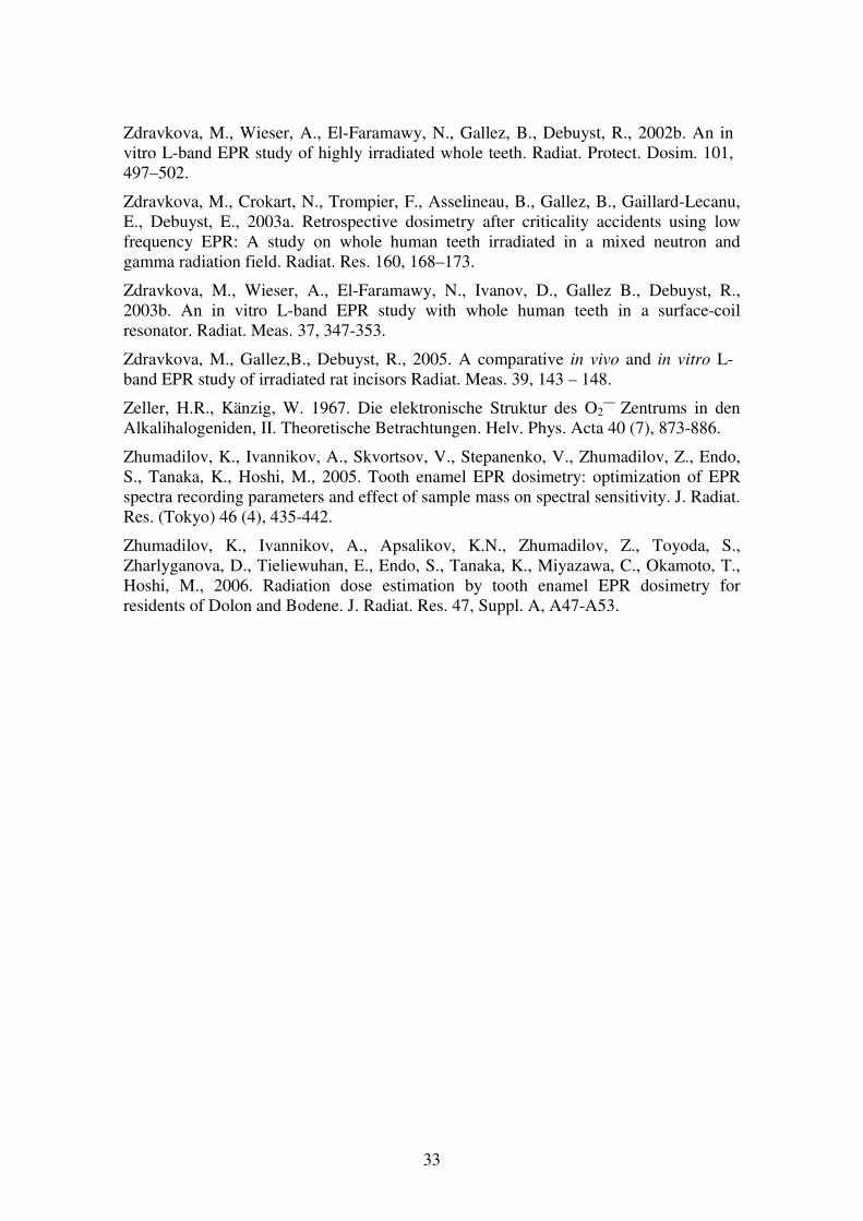
33

Zdravkova, M., Wieser, A., El-Faramawy, N., Gallez, B., Debuyst, R., 2002b. An in vitro L-band EPR study of highly irradiated whole teeth. Radiat. Protect. Dosim. 101, 497–502.

Zdravkova, M., Crokart, N., Trompier, F., Asselineau, B., Gallez, B., Gaillard-Lecanu, E., Debuyst, E., 2003a. Retrospective dosimetry after criticality accidents using low frequency EPR: A study on whole human teeth irradiated in a mixed neutron and gamma radiation field. Radiat. Res. 160, 168–173.

Zdravkova, M., Wieser, A., El-Faramawy, N., Ivanov, D., Gallez B., Debuyst, R., 2003b. An in vitro L-band EPR study with whole human teeth in a surface-coil resonator. Radiat. Meas. 37, 347-353.

Zdravkova, M., Gallez,B., Debuyst, R., 2005. A comparative in vivo and in vitro L-band EPR study of irradiated rat incisors Radiat. Meas. 39, 143 – 148.

Zeller, H.R., Känzig, W. 1967. Die elektronische Struktur des O2— Zentrums in den

Alkalihalogeniden, II. Theoretische Betrachtungen. Helv. Phys. Acta 40 (7), 873-886.

Zhumadilov, K., Ivannikov, A., Skvortsov, V., Stepanenko, V., Zhumadilov, Z., Endo, S., Tanaka, K., Hoshi, M., 2005. Tooth enamel EPR dosimetry: optimization of EPR spectra recording parameters and effect of sample mass on spectral sensitivity. J. Radiat. Res. (Tokyo) 46 (4), 435-442.

Zhumadilov, K., Ivannikov, A., Apsalikov, K.N., Zhumadilov, Z., Toyoda, S., Zharlyganova, D., Tieliewuhan, E., Endo, S., Tanaka, K., Miyazawa, C., Okamoto, T., Hoshi, M., 2006. Radiation dose estimation by tooth enamel EPR dosimetry for residents of Dolon and Bodene. J. Radiat. Res. 47, Suppl. A, A47-A53.

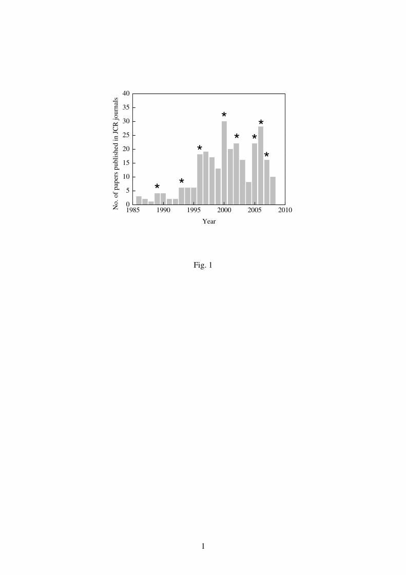
1

1985 1990 1995 2000 2005 20100

5

10

15

20

25

30

35

40

*

* *

***

*N

o.

of

pap

ers

pu

bli

shed

in J

CR

jo

urn

als

Year

*

Fig. 1

2

Fig. 2

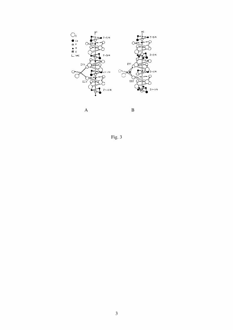
3

A B

Fig. 3

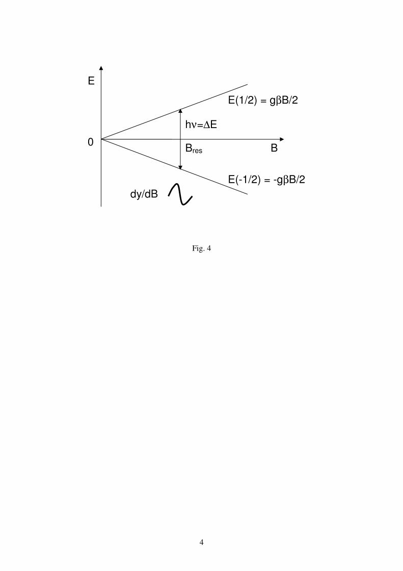
4

Fig. 4

E

0

dy/dBBE

Bres B

E(1/2) = gβB/2

E(-1/2) = -gβB/2

hν=∆E

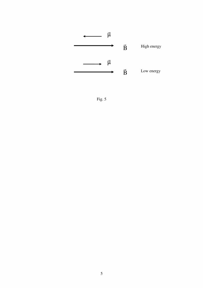
5

Fig. 5

B�

B�

µ�

µ�

High energy

Low energy

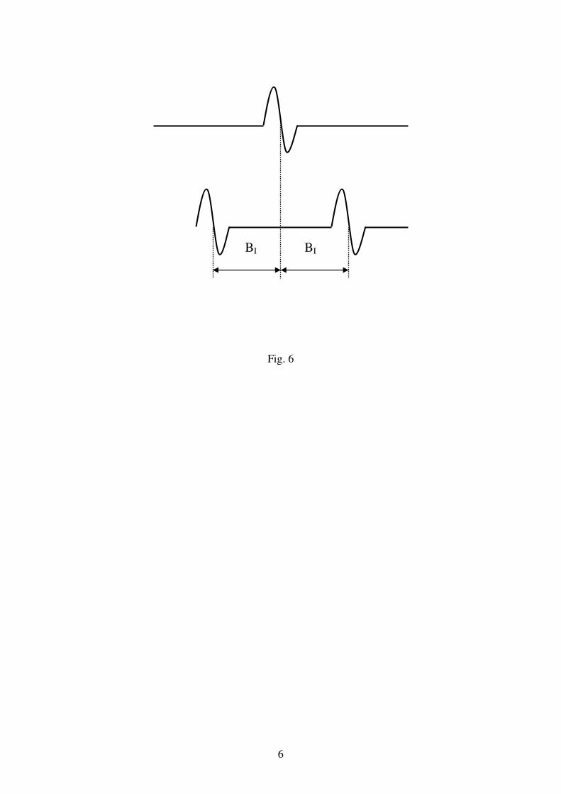
6

Fig. 6

BI BI

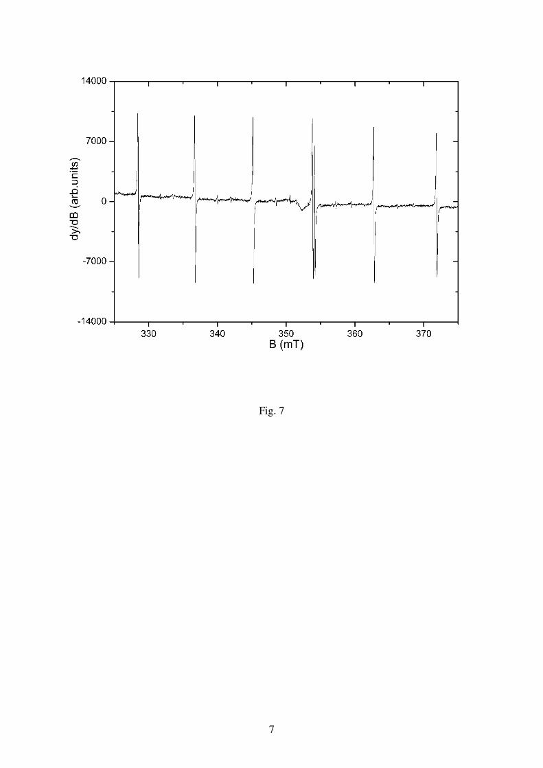
7

Fig. 7

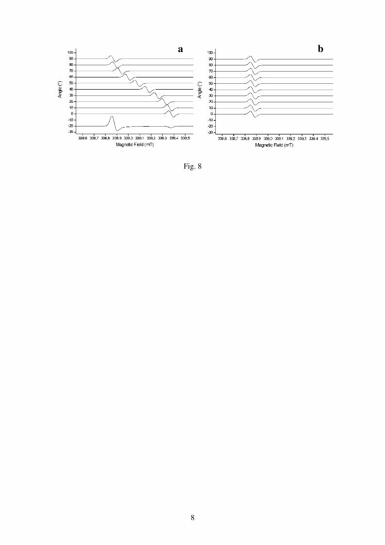
8

Fig. 8

a b

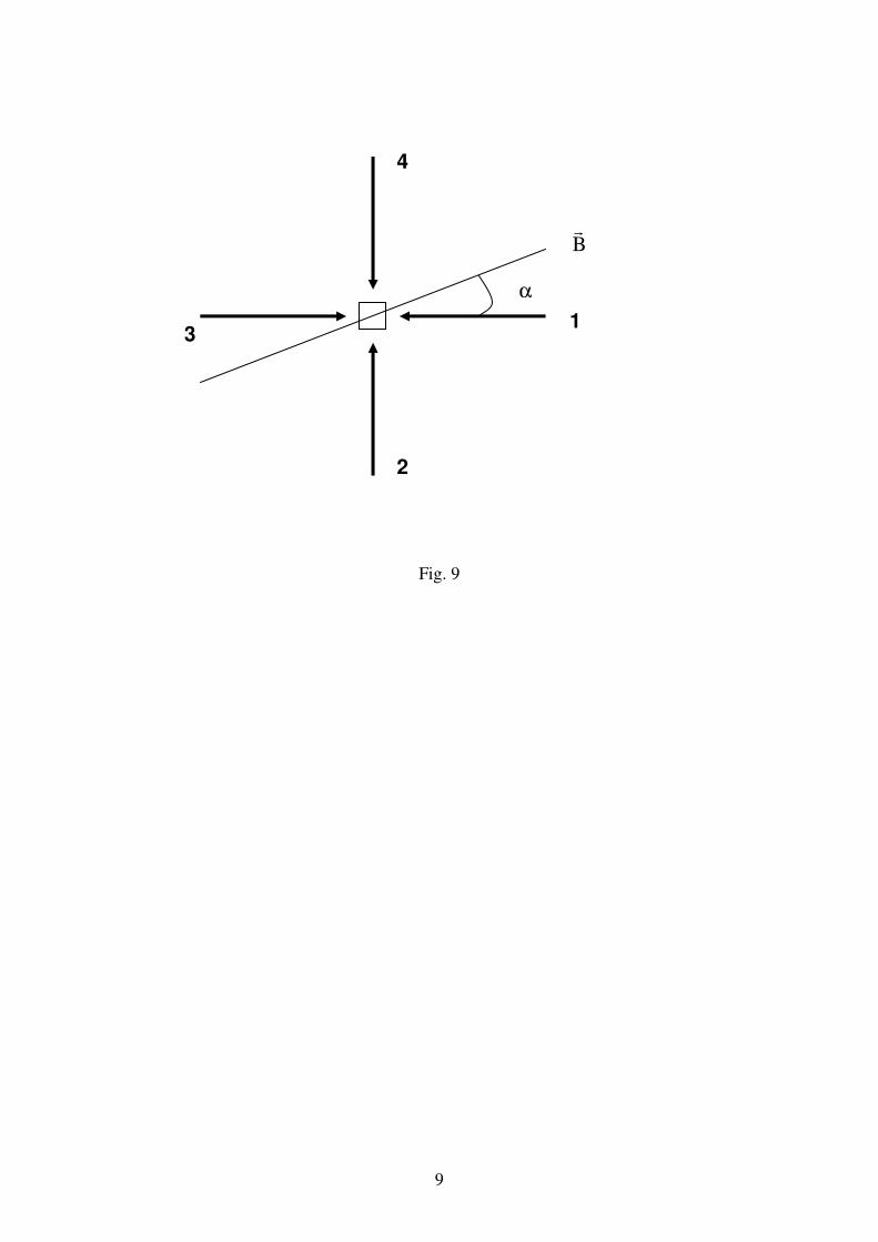
9

Fig. 9

1

2

3

4

B�

1 α

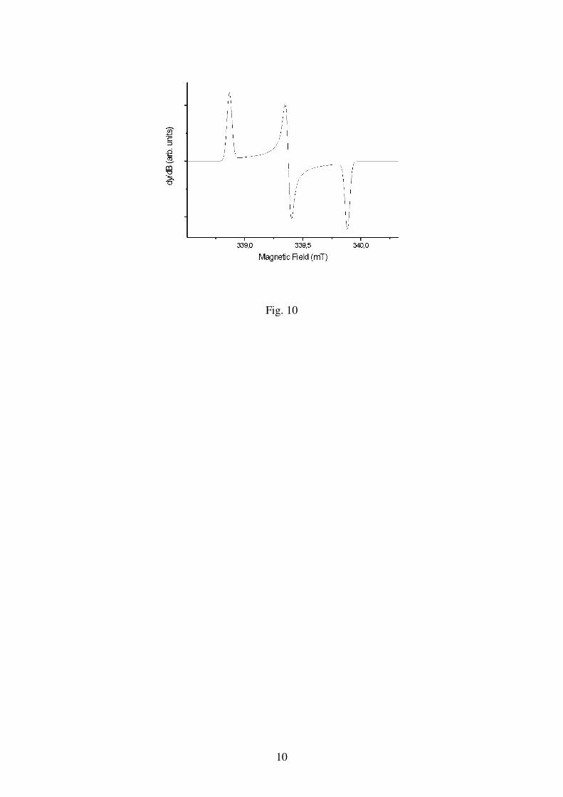
10

Fig. 10

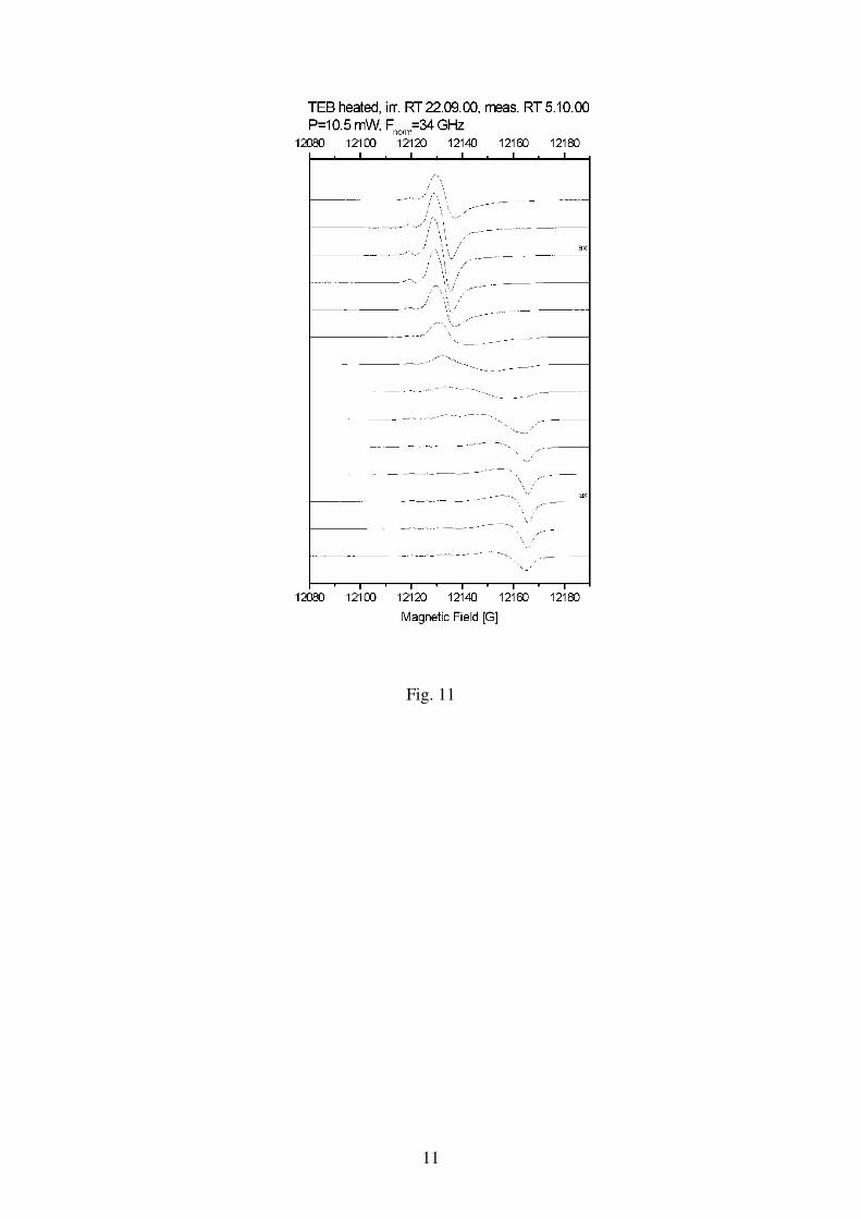
11

Fig. 11

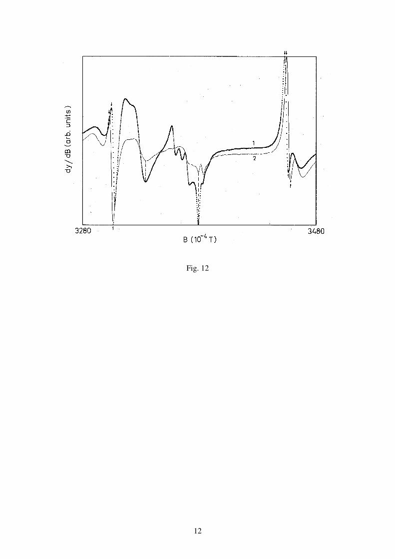
12

Fig. 12

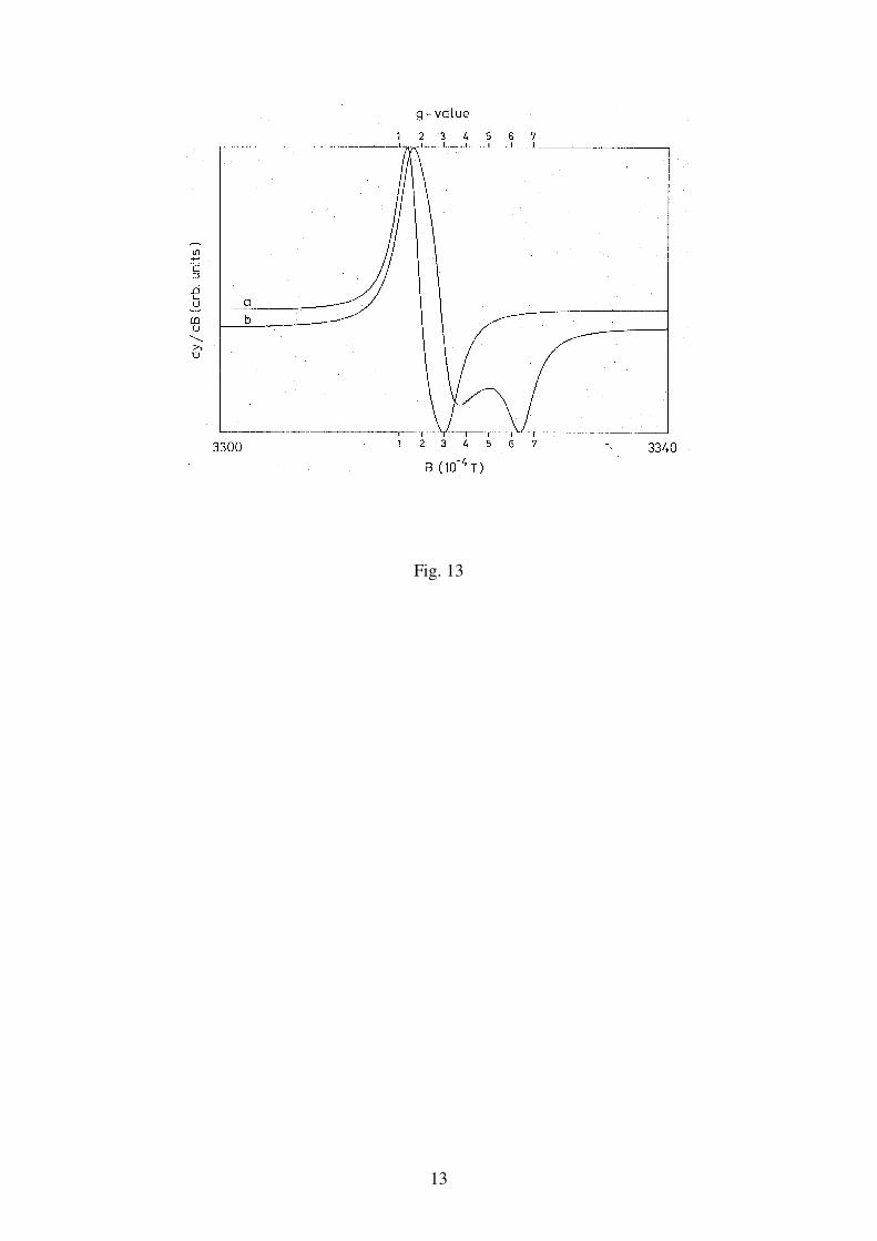
13

Fig. 13

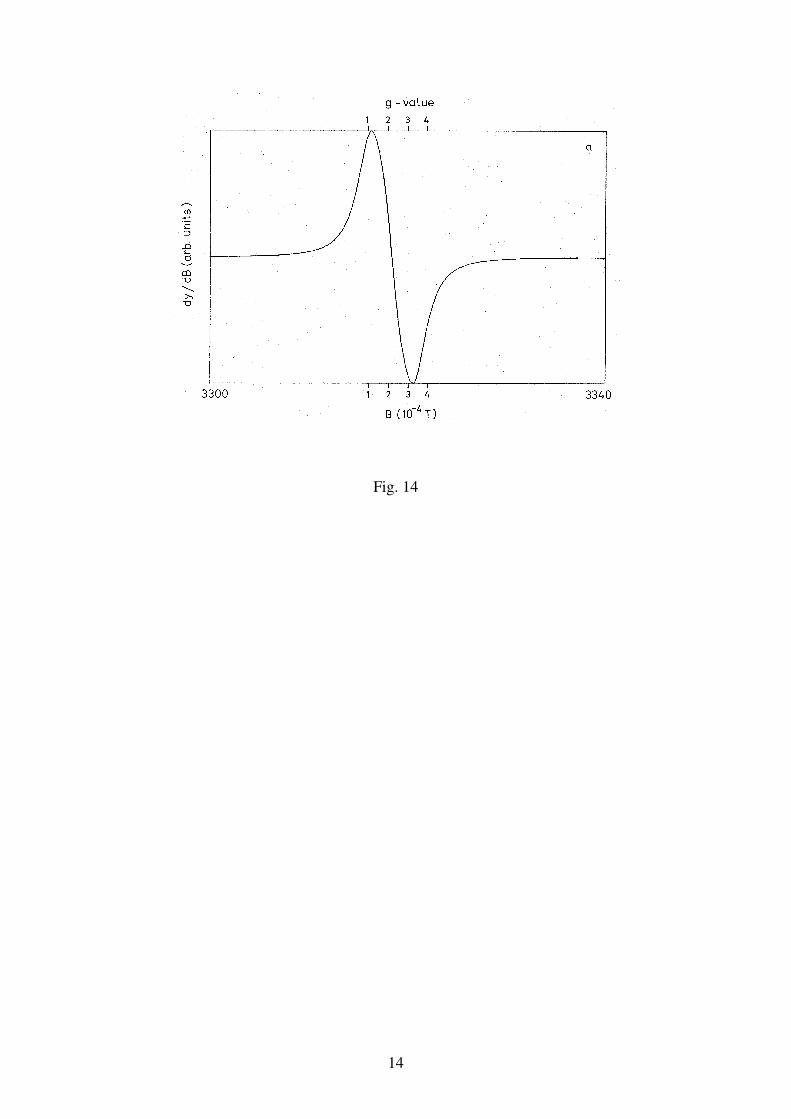
14

Fig. 14

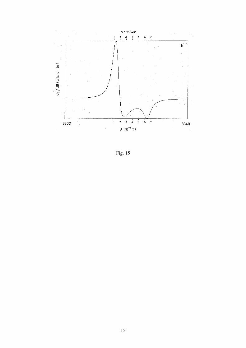
15

Fig. 15

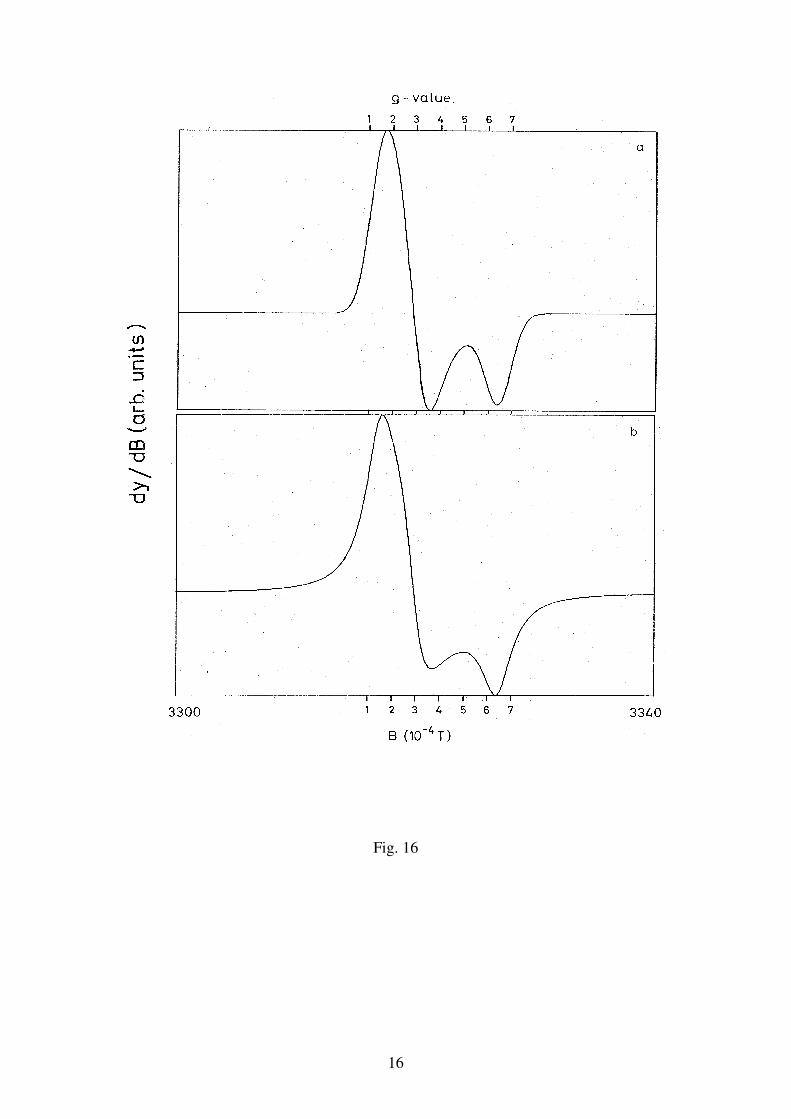
16

Fig. 16

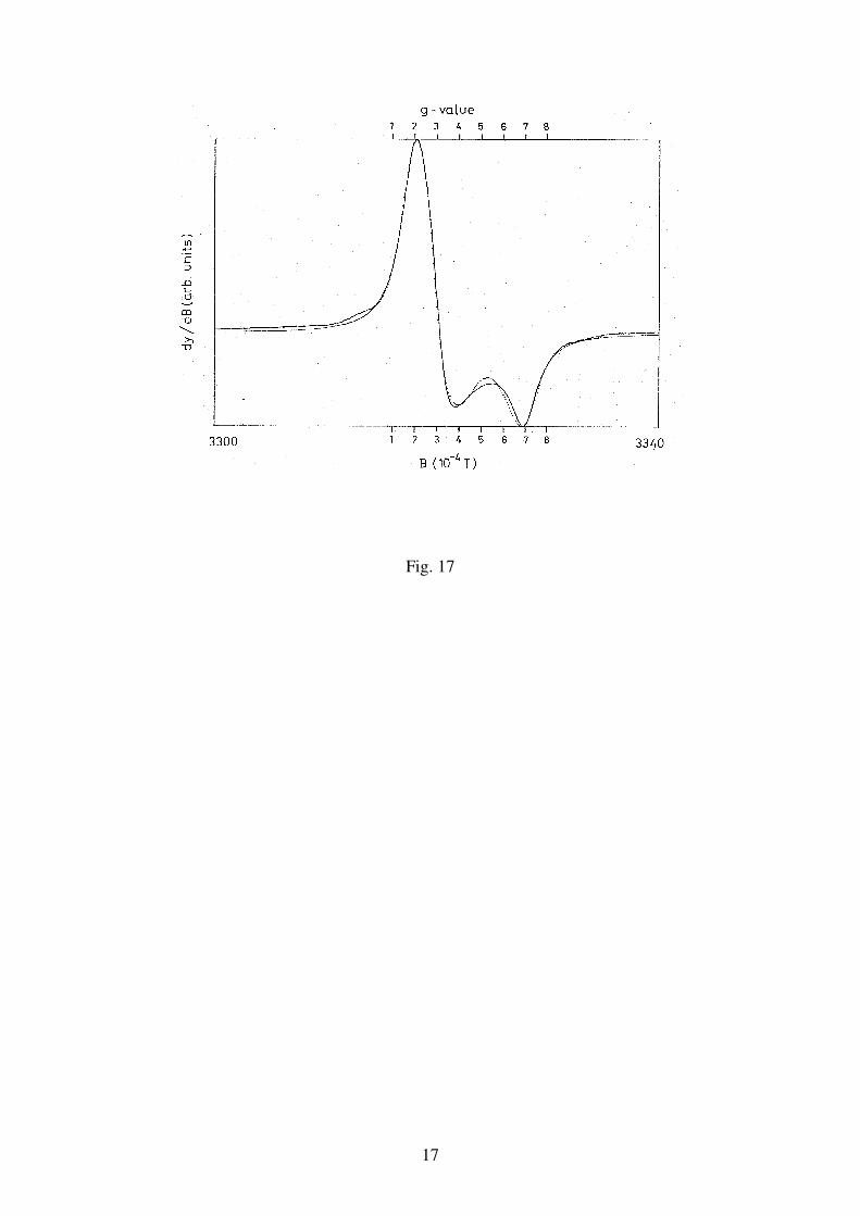
17

Fig. 17

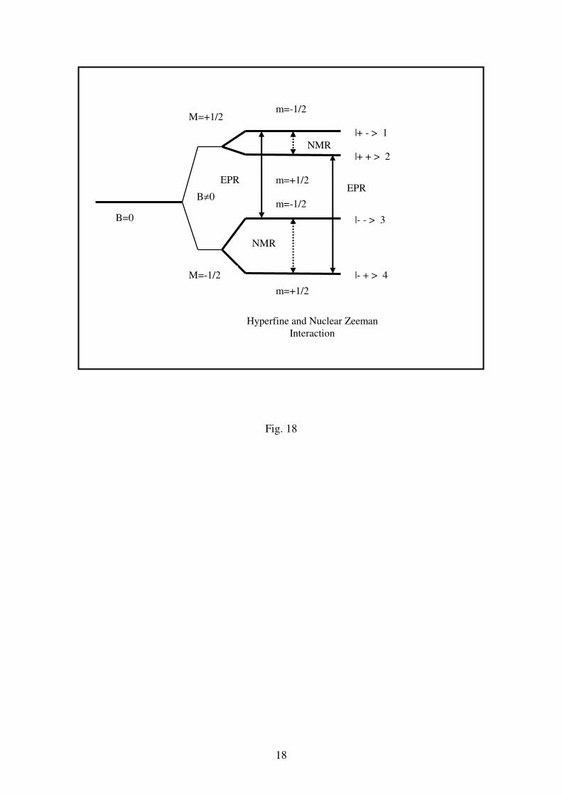
18

Fig. 18

B=0

B≠0

M=+1/2

M=-1/2

m=-1/2

m=+1/2

m=-1/2

m=+1/2

|- + > 4

|+ - > 1

|+ + > 2

|- - > 3

Hyperfine and Nuclear Zeeman Interaction

EPR

NMR

EPR

NMR

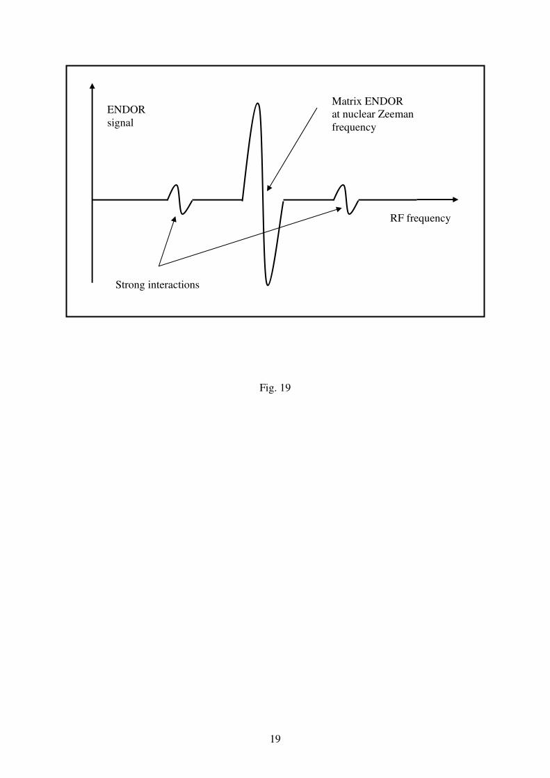
19

Fig. 19

ENDOR signal

RF frequency

Matrix ENDOR at nuclear Zeeman frequency

Strong interactions

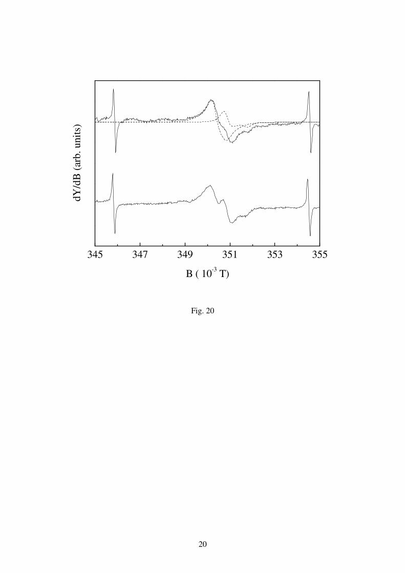
20

345 347 349 351 353 355

dY

/dB

(ar

b.

un

its)

B ( 10-3 T)

Fig. 20

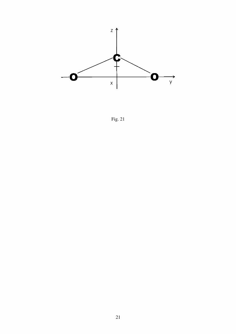
21

Fig. 21

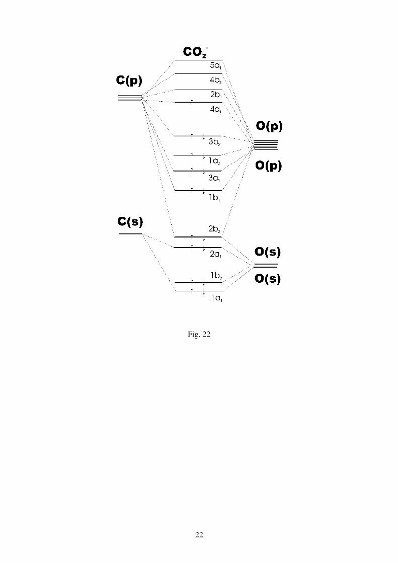
22

Fig. 22

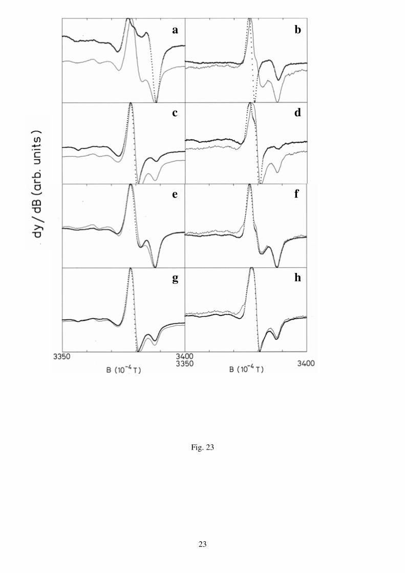
23

Fig. 23

a b

c d

e f

g h

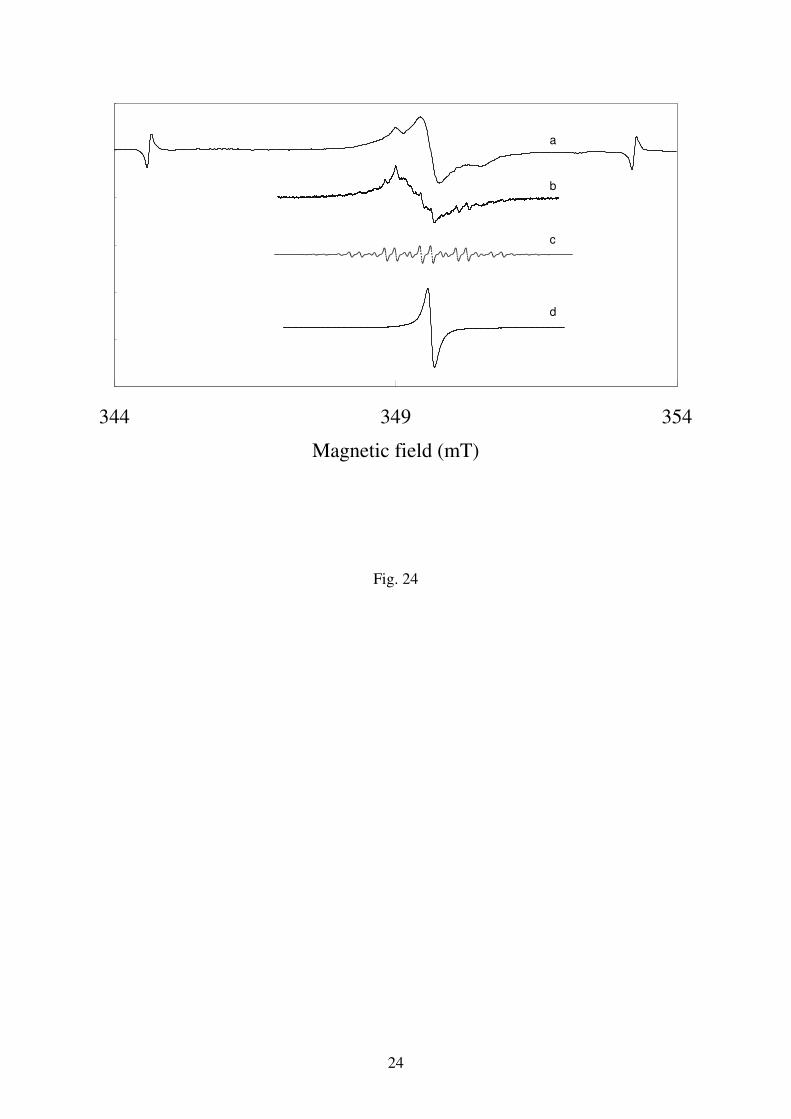
24

344 349 354

Magnetic field (mT)

a

b

c

d

Fig. 24

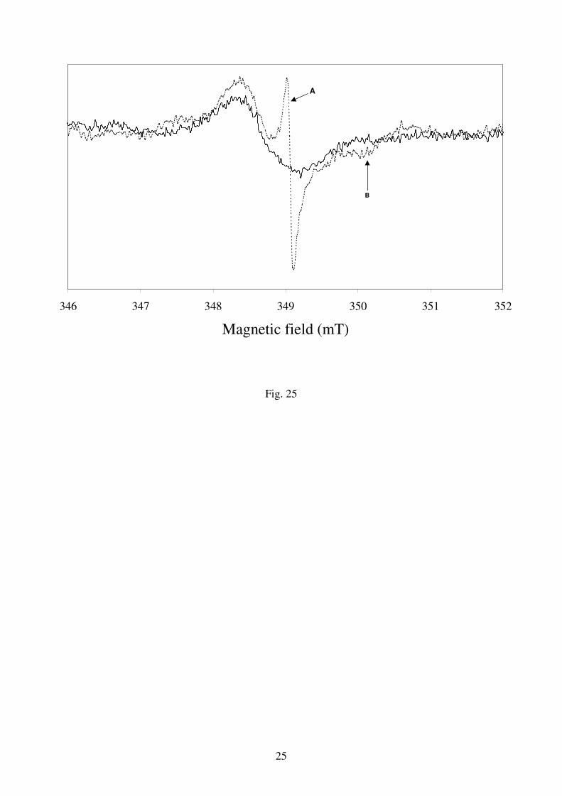
25

Fig. 25

346 347 348 349 350 351 352

Magnetic field (mT)

A

B

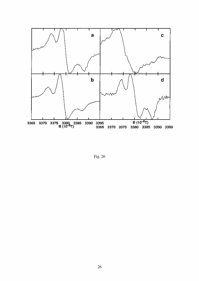
26

Fig. 26

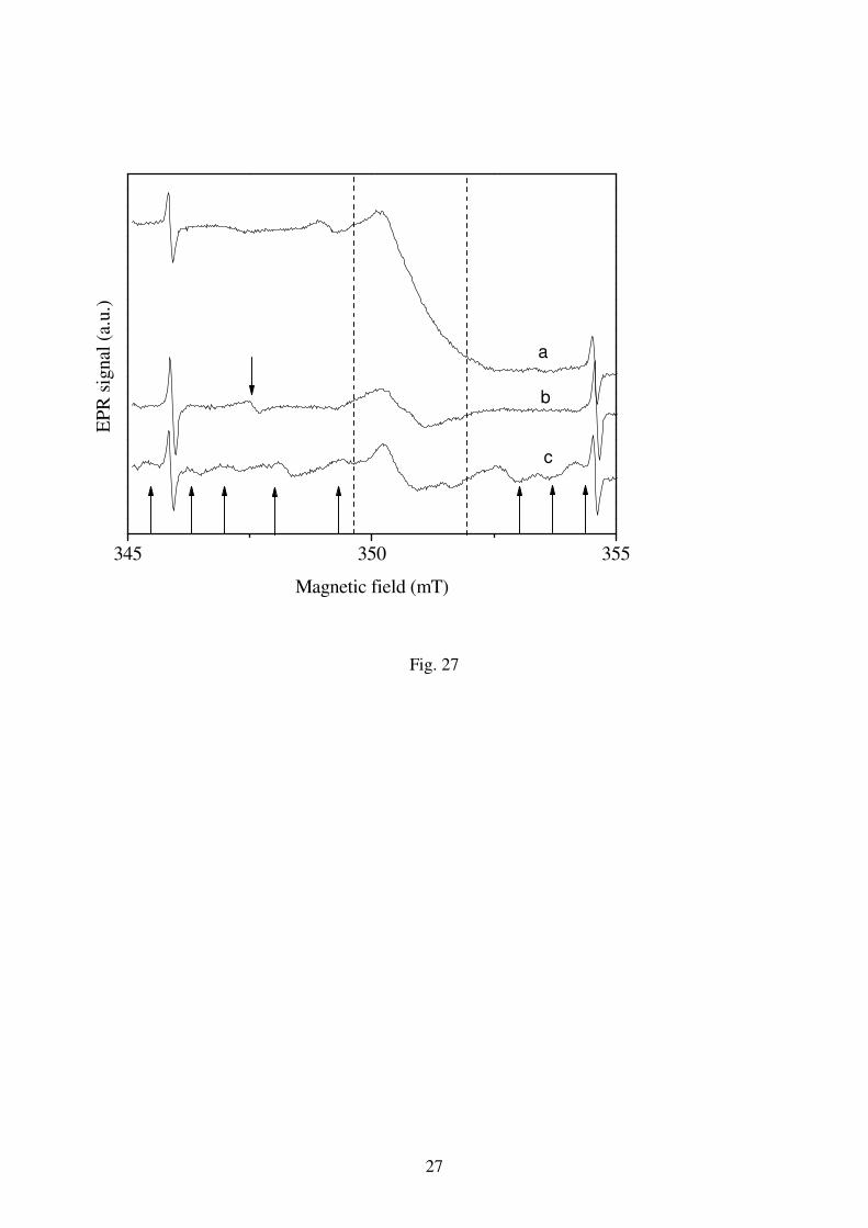
27

Fig. 27

345 350 355

EP

R s

ignal

(a.

u.)

Magnetic field (mT)

a

b

c

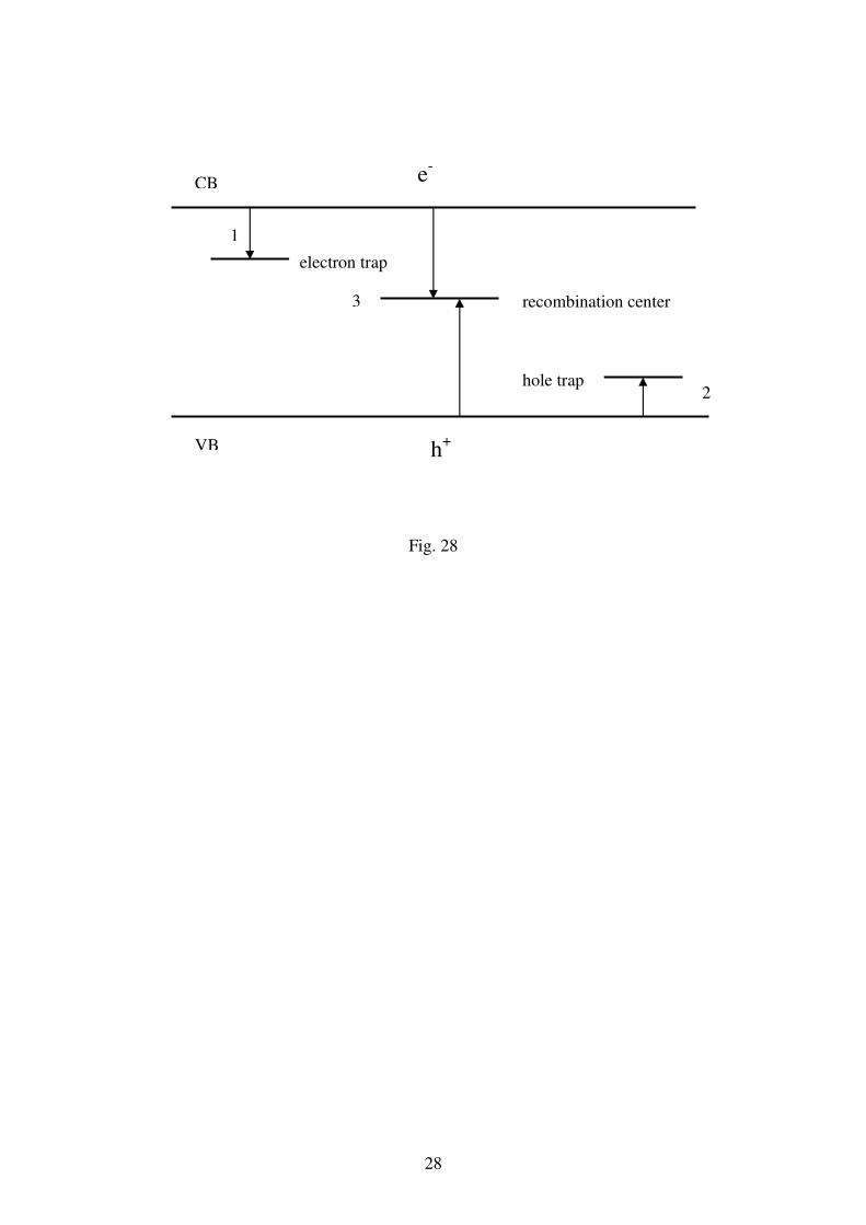
28

Fig. 28

CB

VB

e-

h+

electron trap

hole trap

recombination center

1

2

3

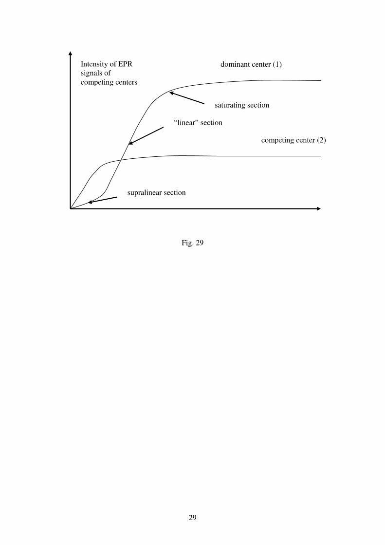
29

Fig. 29

Intensity of EPR signals of competing centers

dominant center (1)

competing center (2)

“linear” section

supralinear section

saturating section

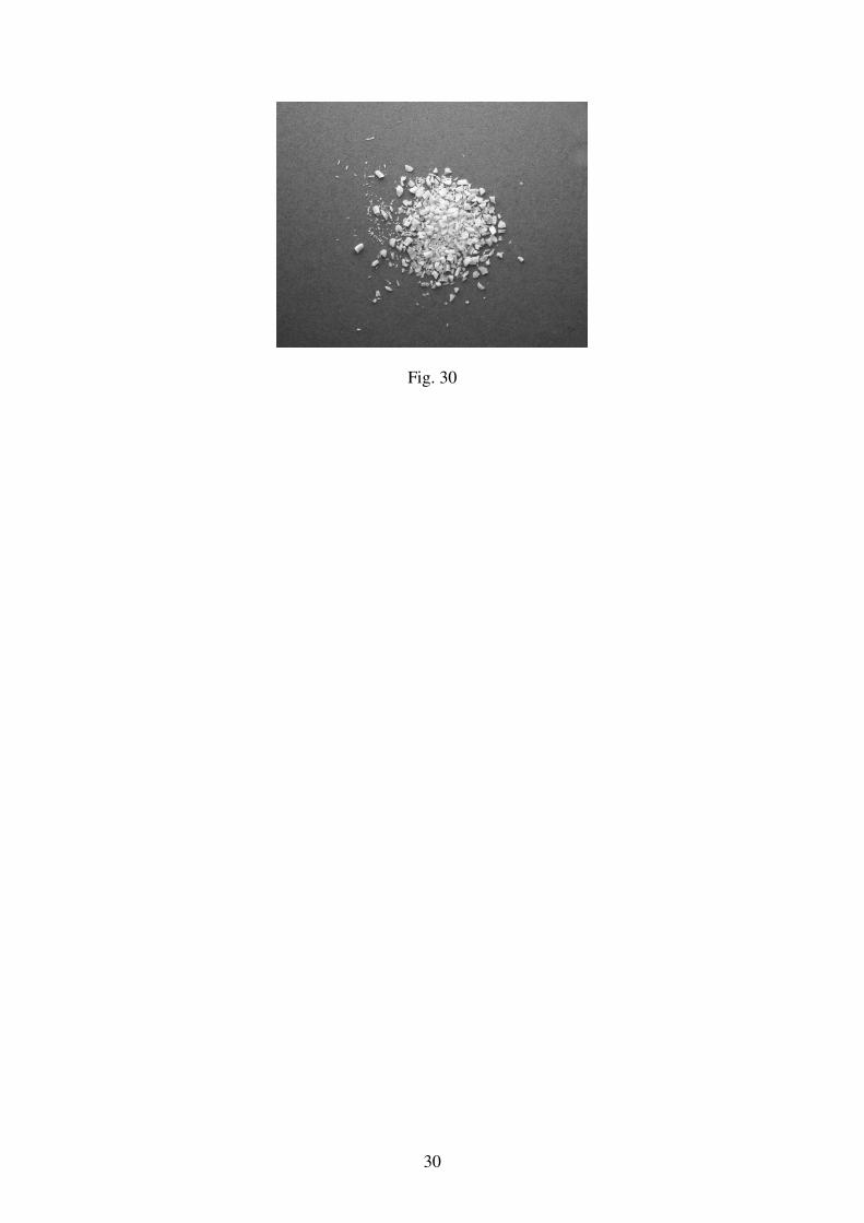
30

Fig. 30

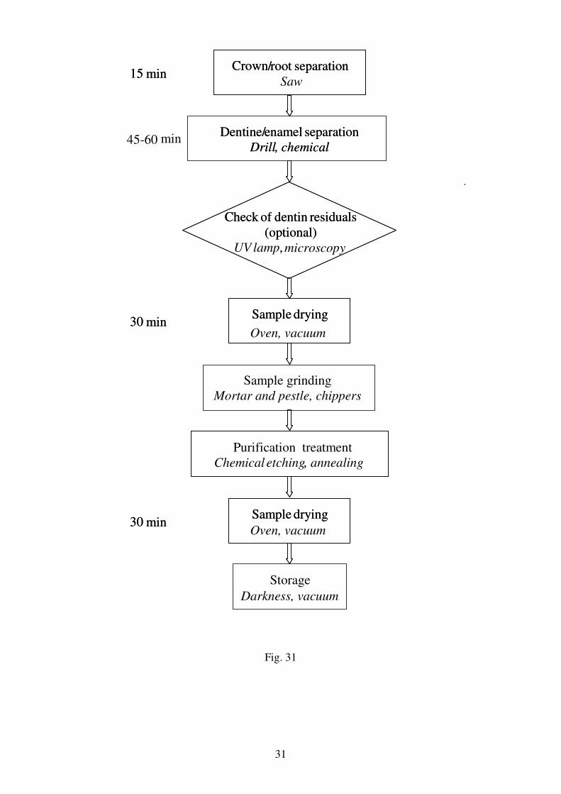
31

Fig. 31

15 min

30 min

30 min

Check of dentin residuals(optional)

UV lamp,

Crown/root separation

Dentine/enamel separationDrill , chemical

Sample drying

Purification treatmentChemical etching , annealing

Sample drying

Storage

15 min

min

30 min

30 min

Check of dentin residuals(optional)

, microscopy

Crown/root separationSaw

Dentine/enamel separationDrill , chemical

Sample drying

Oven, vacuum

Sample grinding Mortar and pestle, chippers

,

Sample drying

Darkness, vacuum

45-60

Oven, vacuum

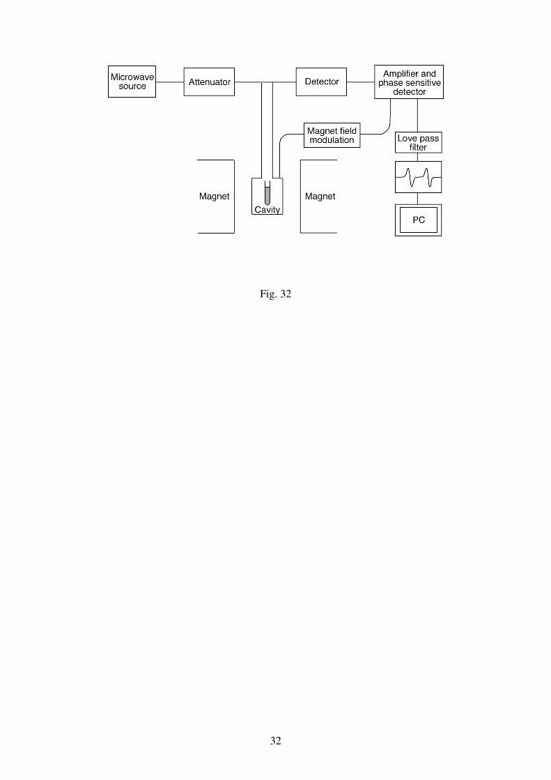
32

Fig. 32

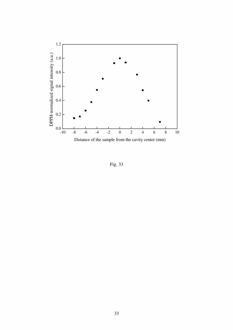
33

-10 -8 -6 -4 -2 0 2 4 6 8 100.0

0.2

0.4

0.6

0.8

1.0

1.2

DP

PH

-no

rmal

ized

sig

nal

in

ten

sity

(a.

u.)

Distance of the sample from the cavity center (mm)

Fig. 33

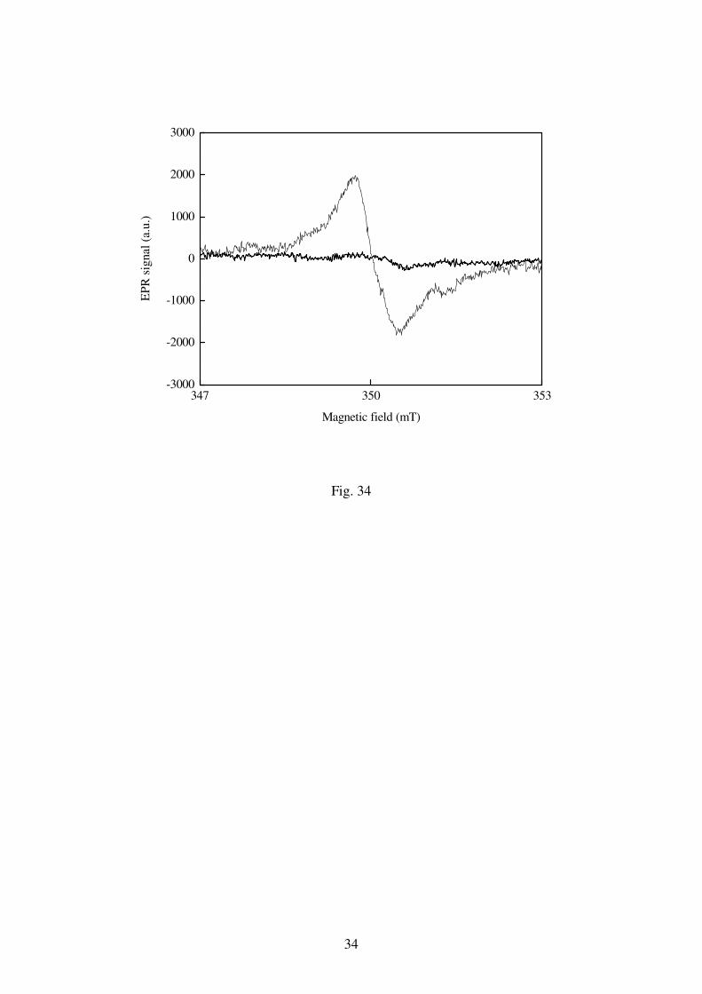
34

347 350 353-3000

-2000

-1000

0

1000

2000

3000

EP

R s

ignal

(a.

u.)

Magnetic field (mT)

Fig. 34

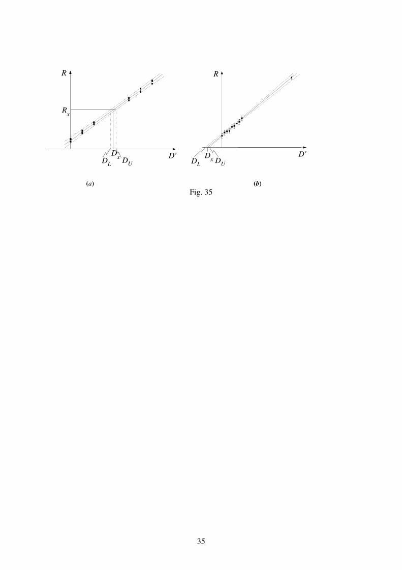
35

D'Dx

Rx

R

DUD

L

D'

R

D

xDL

DU

(a) (b)

Fig. 35

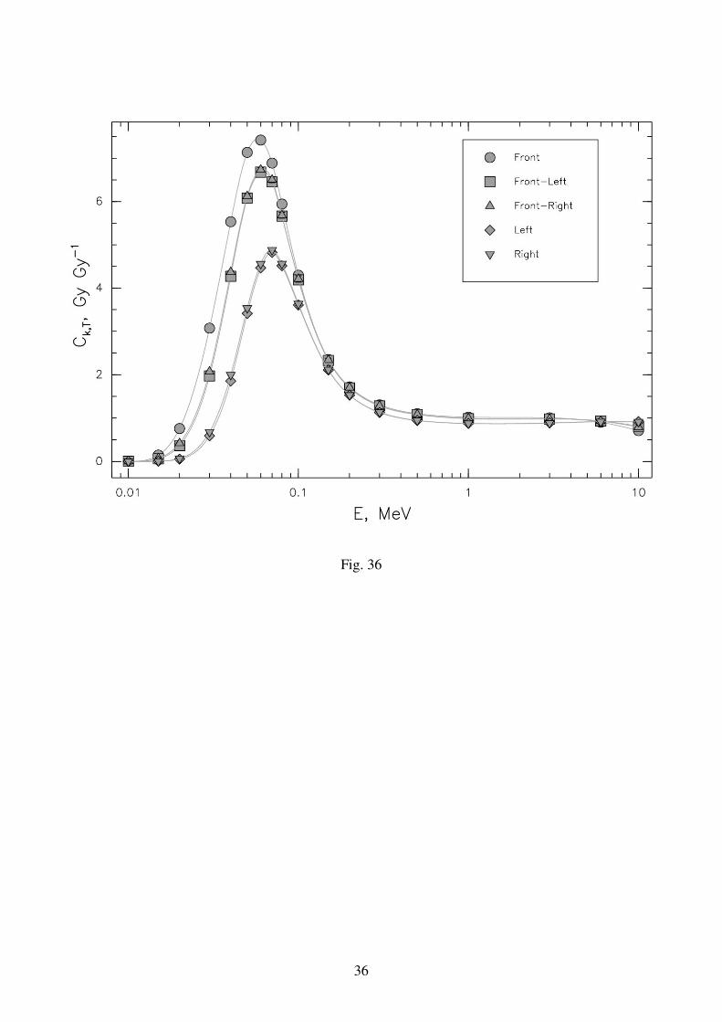
36

Fig. 36

Documents

EPR DOSIMETRY WITH TOOTH ENAMEL: A REVIEW