Available online at www.sciencedirect.com

er.com/locate/eneco

Energy Economics 30 (2008) 1933–1950

www.elsevi

Evaluating the power investment options withuncertainty in climate policy

Ming Yang a,⁎, William Blyth b, Richard Bradley a, Derek Bunn c,Charlie Clarke d, Tom Wilson d

a International Energy Agency, 9, rue de la Fédération, F-75739 Paris Cedex 15, Franceb Oxford Energy Associates, 28 Stile Road, Oxford OX3 8AQ, UKc London Business School, Regent's Park, London NW1 4SA, UK

d Electric Power Research Institute, 3420 Hillview Avenue, Palo Alto, California 94304, USA

Received 26 March 2007; received in revised form 21 June 2007; accepted 21 June 2007Available online 4 July 2007

Abstract

This paper uses a real options approach (ROA) for analysing the effects of government climate policyuncertainty on private investors’ decision-making in the power sector. It presents an analysis undertaken by theInternational Energy Agency (IEA) that implements ROA within a dynamic programming approach fortechnology investment choice. Case studies for gas, coal and nuclear power investment are undertaken with themodel. Illustrative results from the model indicate four broad conclusions: i) climate change policy risks canbecome large if there is only a short time between a future climate policy event such as post-2012 and the timewhen the investment decision is being made; ii) the way in which CO2 and fuel price variations feed through toelectricity price variations is an important determinant of the overall investment risk that companies will face; iii)investment risks vary according to the technology being considered, with nuclear power appearing to beparticularly exposed to fuel and CO2 price risks under various assumptions; and iv) the government will be ableto reduce investors' risks by implementing long-term (say 10 years) rather than short-term (say 5 years) climatechange policy frameworks. Contributions of this study include: (1) having created a step functionwith stochasticvolume of jump at a particular time to simulate carbon price shock under a particular climate policy event; (2)quantifying the implicit risk premium of carbon price uncertainty to investors in new capacity; (3) evaluatingcarbon price risk alongside energy price risk in investment decision-making; and (4) demonstrating ROA to be auseful tool to quantify the impacts of climate change policy uncertainty on power investment.© 2007 OECD/IEA. Published by Elsevier B.V. All rights reserved.

JEL classification: F53; C61; D78; E37; G18; O16; O38; Q48; Q52; Q54

Keywords: Real options; Investment; Uncertainty; Carbon shock; Climate policy

⁎ Corresponding author. Tel.: +33 1 40 57 67 33; fax: +33 1 40 57 67 39.

E-mail address: ming.yang@iea.org (M. Yang).

0140-9883/$ - see front matter © 2007 OECD/IEA. Published by Elsevier B.V. All rights reserved.doi:10.1016/j.eneco.2007.06.004

1934 M. Yang et al. / Energy Economics 30 (2008) 1933–1950

1. Introduction

Investment in the power sector has at least three crucial characteristics. Firstly, the investment ispartially or completely irreversible. Once invested, the asset may become stranded because ofvarious risks. Secondly, without hedging, the price risks, market evolution and policy interventionuncertainties can have a substantial effect on financial performance. Thirdly, without centralplanning, the timing of an investment is discretionary. Profit-seeking enterprises can invest in apower plant now if they think the return on the investment is high enough to match the risks, or theycan postpone the investment to acquire more information on some of those risks. In other words,investors have the option but not the obligation to invest in a project at a particular point in time.

Furthermore, because different technologies emit different amounts of greenhouse gases perunit of electricity generated, climate policy risk introduces a new factor into this investmentdecision. Whether climate change policies are introduced through a price mechanism (e.g., permittrading scheme or carbon tax) or through some other regulatory mechanism, the current andpotential future cost of emissions needs to be included in the investment analysis, even incountries where there is currently no cost for emitting greenhouse gases. One problem withincorporating these emission costs into financial appraisal is that the status of climate changepolicy in most countries is uncertain. Uncertainties range from general issues such as whether /when carbon constraints will be imposed to more specific issues the form of regulation, stringencyof emissions controls and levels of allocation of emission permits. Confounding this issue,volatile oil prices not only add their own uncertainties into the equation, but influence the relativecosts of carbon abatement opportunities.

The objective of this paper is to present the results of quantifying the cost of uncertainty in theprocess of climate policy evolution, through its effects on inducing greater optionality considerationsin the behaviour of investors. The paper provides some illustrative results for the choice between coaland gas (with and without carbon capture) as well as nuclear power plants.

2. Methodology

2.1. Real options approach

The term “real options approach” (ROA) can be traced to Myers (1977), who first identifiedthe analogy between investments in real assets and financial options. ROA is useful in projectappraisal when the project revenue streams resulting from the investment are uncertain, whenthere is the possibility of learning about future market conditions that could affect the project'sprofitability, and when there is the possibility to optimally choose the time to make theinvestment. A number of studies have been undertaken applying ROA to evaluate power projectinvestments. Laughton et al. (2003) applied this approach to assessing geological greenhouse gassequestration. They concluded that the use of a traditional deterministic discounted cash flow(DCF) can distort the valuation of projects, as it does not account for the complex effects of riskand uncertainty. Using ROA in an environment of uncertain CO2 price, Sekar (2005) evaluatedinvestments in three coal-fired power generation technologies: pulverized coal, standardIntegrated Coal Gasification Combined Cycle (IGCC) and IGCC with pre-investments to reducethe cost of future CCS retrofitting. Sekar developed cash flow models for each of the threetechnologies, with CO2 price as an uncertain variable. Rothwell (2006) used ROA techniques toevaluate risks to the development of new nuclear power plants. He modeled three uncertainties:price risk, output risk and cost risk. Using a Monte Carlo simulation, Rothwell derived various

1935M. Yang et al. / Energy Economics 30 (2008) 1933–1950

risk premiums, between $383/kW and $751/kW that would trigger investment in the UnitedStates' new nuclear power plants.

Laurikka (2006) presented a simulation model using ROA to quantify the value of IntegratedGasification Combined Cycle (IGCC) technology within an emissions trading scheme. The studydesigned and simulated three types of stochastic variable: the price of electricity, the price of fueland the price of emission allowances. Laurikka concluded, (1) a straightforward application of thetraditional project appraisal on a scenario of IGCC can bias results for current competitive energymarkets regulated by an emissions trading scheme; (2) the potential combination of severaluncertainties rendered the European Union Emission Trading Scheme (EU ETS) complex; and (3)when accounting for uncertainties, the IGCC technology is not competitive within the EU ETS.

Lin et al. (2007) used the ROA to examine how much and when greenhouse gas emissionsshould be reduced in a case study. On the basis of a detailed literature review on the ROA, theycreated a simple mathematical model for assessing environmental pollution prevention whenecological and economic uncertainty coexists, which may provide a reference or a foundation forgovernment decision making. They studied the optimum timing for adopting pollution preventionpolicies by expanding the continuous time model of decision making for the greenhouse effect,taking into account environmental and economic uncertainty. One of the interestingly specificquantifications of Lin et al. (2007) is that they presented a case study in which decision makersadopt a pollution prevention policy when the pollutants reach a particular threshold of 48 milliontons. This illustrates the nature of ROA in providing a framework for understanding decisiontriggers as environmental scenarios evolve.

Other recent applications of ROA in the energy sector include (1) Siddiqui et al. (2007), whoevaluated the United States' federal strategy for renewable energy research, development,demonstration, and development; (2) Marreco and Carpio (2006), who examined the flexibility ofthe Brazilian power system; and (3) Kuper et al. (2006), who evaluated the influence of uncertainoil prices on energy use.

The Electric Power Research Institute of the USA (EPRI, 1999) developed the GreenhouseGas Emission Reduction Analysis Model to evaluate the revenues, costs and expected after-taxgross margin accruing from investment in the technology of greenhouse gas reduction. The modelincorporates Monte Carlo simulation, and methods of the ROA to enable an evaluation of specificGHG reduction strategies that account for individual risks and uncertainties. The modelincorporates energy prices and CO2 prices with correlations. Developed in an MS Excelenvironment, the model is supported by a semi-commercial software program for calculating realoptions, which is also the basis for the work described in this paper.

2.2. Modelling climate policy uncertainty and investment risk

In the work reported in this paper, the ROA has been used to evaluate the risks associated withuncertainty in climate change policy with an ultimate view to making recommendations on howpolicy could be implemented to reduce investment risk. The approach provides a useful basis forpolicy analysis, as it effectively allows different risk factors to be considered individually or incombination, so that the effects of policy risk, as distinct from market risk, can be isolated. Thereal options we investigate here are related to the flexibility that companies have to optimally timetheir investment in the face of regulatory uncertainty — in other words to delay their investmentwith the prospect of gaining better information regarding the likely outcome of the policydecisions. The ability for investors to improve likely project outcomes by waiting for additionalinformation means that project returns for investments which go ahead immediately (i.e., thereby

1936 M. Yang et al. / Energy Economics 30 (2008) 1933–1950

absorbing the regulatory risk), need to be correspondingly higher in order to overcome this‘option value of waiting’. In this work, we therefore use the value of waiting as a measure of risk.Climate change policy uncertainty is represented in the investment decision by means of anuncertain carbon price. In reality, climate policy may take several forms, and does not necessarilyset a direct carbon price. Nevertheless, climate policies will impose costs on investors, and wemake the convenient modelling assumption that these can be represented in total as an equivalentcarbon price. Some elements of policy risk are missed out as a result of this simplification. Forexample, in an emissions trading scheme, there may be uncertainty not only concerning the priceof carbon, but also the level of free allocation of allowances. In this study, we did not take intoaccount the effects of free allocation on the investment decision — i.e. we effectively assumed100% auctioning of allowances. In principle, the approach outlined below could be extended toinclude the effects of free allocation as a subsidy to fossil-fuel generation technologies and tomodel the effects of allocation uncertainty as a source of risk for these plant going forward.

To capture energy market uncertainty, fuel prices are also taken to be stochastic, and variousassumptions are made about price variability and correlation between the different uncertainvariables. Fuel price uncertainty is included in the model in order to provide a comparison withcarbon price uncertainty. We do not however model the full range of investment risks. For exampletechnical risks such as capital cost uncertainty and demand / load factor uncertainty are not included.Again, in principle such sources of uncertainty could be incorporated into an extended ROA.

2.3. Modelling real options with dynamic programming

The approach we have taken is an optimisation of investment decision-making under uncertaintyusing dynamic programming, as described for example in Dixit and Pindyck (1994). The dynamicprogramming compares the expected outcome of investing in a project in the current year with analternative (‘continuation value’) which delays investment until the timing is optimal. The calculationof the continuation value requires solving the problem from the final year of the scenario, workingbackwards to the first year in order to deduce the optimal investment rule over the whole possibleinvestment horizon.

This can be described mathematically as follows. We consider a project with lifetime L which canbe irreversibly initiated in any year t (0b tbT) for a total capital outlay of K. The cash-flow in year twithout the investment isAt, and the annual cash-flow with the investment isBt. Since these values areuncertain, the project value will depend on the expectation E[.] of these values. The total net presentvalue Vt

inv of the project if investment goes ahead in year t is:

V invt ¼

XLn¼t

dðt; nÞE½Bn� !

� K ð1Þ

where d(t,n) denotes the discount factor applied at time t to cash flows occurring at time n. Thecontinuation valuewhich is the net present value of the project if one chooses not to invest in the projectat period t (but assuming optimal investment opportunity depending on future conditions) is given by:

V contt ¼ At þ dðt; t þ 1ÞE½V ⁎

ðtþ1Þ� ð2Þ

where V⁎ is the optimal net present value of the project cash flows from year t+1 until the end of theproject lifetime under the assumption of optimal investment behaviour. The assumption of optimalinvestment behaviour in future years requires the comparison of Vinv with Vcont in every future year.

1937M. Yang et al. / Energy Economics 30 (2008) 1933–1950

Since the continuation value always depends on the total expected value of the project in the followingyear, this procedure needs to be solved from the end of the project, working backwards. The finalpossible year for investing in the project is year T, at which it is assumed that the decision is a ‘now ornever’ investment choice. In year T, Vinv becomes the expected value of the project over its lifetime,and Vcont equals zero (since there is no further opportunity to invest beyond this date). Investment willtherefore go ahead in year T if VT

invN0.From the perspective of year T−1, the decision in year Twill depend on the random changes

in variables in the intervening year. Therefore the continuation value will be based onexpectations in year T−1 which we denote ET−1[.]. In year T−1, the continuation value becomesthe current year's income AT−1 plus the discounted value of the expected project value given theexpected outcome of the decision in year T, and the current state of information in year T−1.

V contT�1 ¼ AT�1 þ dðT � 1; TÞmaxfET�1½V inv

T �; 0g ð3ÞOnce the continuation value in year T−1 has been calculated, this provides a minimum value

which VT−1inv must exceed in order for investment to proceed in that year. This provides an optimal

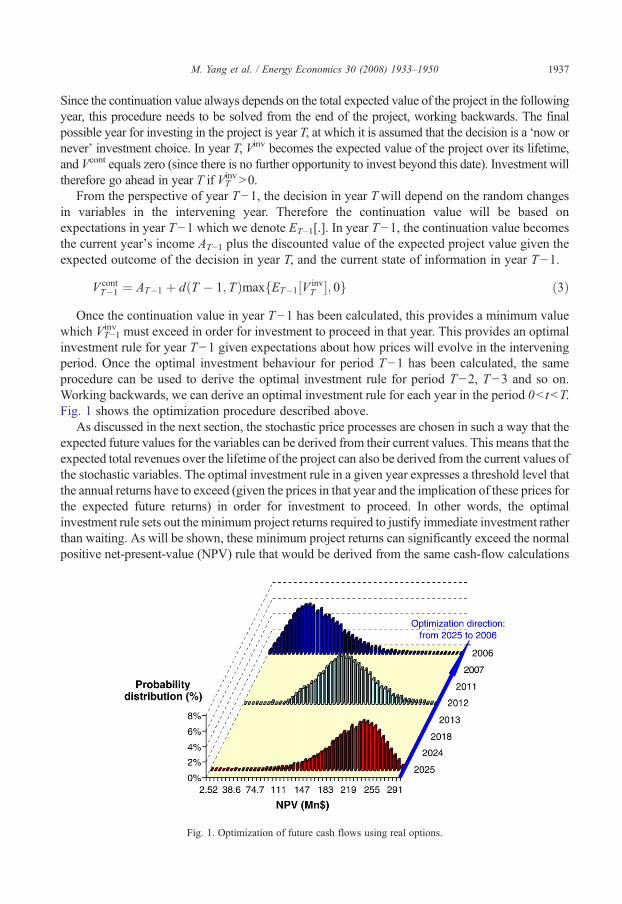
investment rule for year T−1 given expectations about how prices will evolve in the interveningperiod. Once the optimal investment behaviour for period T−1 has been calculated, the sameprocedure can be used to derive the optimal investment rule for period T−2, T−3 and so on.Working backwards, we can derive an optimal investment rule for each year in the period 0b tbT.Fig. 1 shows the optimization procedure described above.

As discussed in the next section, the stochastic price processes are chosen in such a way that theexpected future values for the variables can be derived from their current values. This means that theexpected total revenues over the lifetime of the project can also be derived from the current values ofthe stochastic variables. The optimal investment rule in a given year expresses a threshold level thatthe annual returns have to exceed (given the prices in that year and the implication of these prices forthe expected future returns) in order for investment to proceed. In other words, the optimalinvestment rule sets out the minimum project returns required to justify immediate investment ratherthan waiting. As will be shown, these minimum project returns can significantly exceed the normalpositive net-present-value (NPV) rule that would be derived from the same cash-flow calculations

Fig. 1. Optimization of future cash flows using real options.

1938 M. Yang et al. / Energy Economics 30 (2008) 1933–1950

under certainty. The degree to which the optimal investment rule exceeds the standard positive NPVrule is a measure of the option value of optimising investment timing. It can also be interpreted as ameasure of the risk premium that could be incorporated into investment decision-making as a resultof price uncertainty. This risk premium can further be expressed as $/kW at an additional cost ofconstruction for investors and/or as surcharges in cents/kWh for electricity end-users.

2.4. Overall model structure

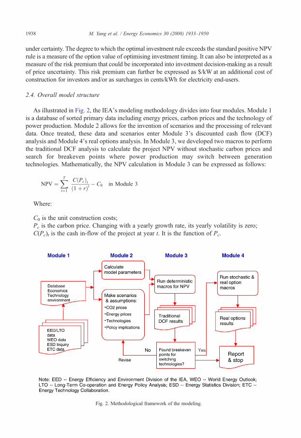
As illustrated in Fig. 2, the IEA's modeling methodology divides into four modules. Module 1is a database of sorted primary data including energy prices, carbon prices and the technology ofpower production. Module 2 allows for the invention of scenarios and the processing of relevantdata. Once treated, these data and scenarios enter Module 3's discounted cash flow (DCF)analysis and Module 4's real options analysis. In Module 3, we developed two macros to performthe traditional DCF analysis to calculate the project NPV without stochastic carbon prices andsearch for breakeven points where power production may switch between generationtechnologies. Mathematically, the NPV calculation in Module 3 can be expressed as follows:

NPV ¼XTt¼1

CðPcÞtð1þ rÞt � C0 in Module 3

Where:

C0 is the unit construction costs;Pc is the carbon price. Changing with a yearly growth rate, its yearly volatility is zero;C(Pc)t is the cash in-flow of the project at year t. It is the function of Pc.

Fig. 2. Methodological framework of the modeling.

1939M. Yang et al. / Energy Economics 30 (2008) 1933–1950

In the model, different electricity and carbon prices drive the module running the search. Oncethe critical points of technology switching appear, the correlating CO2 price and other data arerecorded for reporting and fed into the next module for ROA model running.

In Module 4, while setting the CO2 and energy prices to change randomly, we calculatethe stochastic NPVs for all candidate technologies in each of the planning years. Thefollowing formula is used in Module 4 to calculate the project stochastic NPV:

NPV ¼XTt¼1

CðStochastic Pc and PeÞtð1þ rÞt � C0 in Module 4

Where:

C0 is the unit construction costs;Pc and Pe are the carbon prices and energy prices. They change stochastically in the model;C(Stochastic Pc and Pe)t is the cash in-flow of the project at year t. It is the function of Pc andPe.

We then run the real options calculator, a commercial software programme of real optionsanalysis following the rule of optimization described in Eqs. (1)–(3) above to produce the optimalinvestment options for different technologies during different years. Finally, by comparing theresults from Modules 3 and 4, we estimate the risk premiums in the energy sector investments. Inthe following section, we describe in more details about our cash flow model for NPV calculationand risk premium calculation.

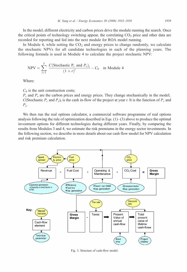
Fig. 3. Structure of cash-flow model.

1940 M. Yang et al. / Energy Economics 30 (2008) 1933–1950

The structure of the NPV cash flow model shown in Fig. 3 looks similar to that of a usualproject appraisal cash flow model. It derives the project net present value by calculating thefollowing cash flow elements: (1) revenue; (2) fuel cost; (3) operation and maintenance costs; (4)CO2 costs; (5) tax payment; and (6) investment capital. Fig. 3 also shows where the energy marketvariables and technical parameters are fed in the model to calculate the cash-flow elements.Energy market variables include energy prices and the costs of capital for various powergeneration technologies. The technical parameters include the plant lifetime (e.g. assumed to be25 years for a gas plant, 40 years for a coal plant), fuel consumption per unit of kWh generation,CO2 emissions per kWh of output, and capacity factor assumptions for the power plants.

The model measures the total revenues minus the total operating costs adjusted for tax and buildtime and discounted to give the total present value of cash-flows over the expected lifetime of theplant. For simplicity, this final output from the cash flow is referred to from here on as the grossmargin. If this gross margin is larger than the capital costs for the investment, the NPV would bepositive. However, this does not necessarily indicate that the project would go ahead. Rather, theinvestment will only go ahead if the expected value of the project exceeds the continuation value inany given year of the scenario. In general, the greater the level of uncertainty, the greater thecontinuation value, since the range of possible future values of the project will be greater, and so thepossibility to optimise the value of the project through delay will be greater.

There are three key characteristics in this model that make its results significantly different fromothers. First, energy price and CO2 price are evolved asMonte Carlo variables. Each of them can beset individually as a random variable, or both of them simultaneously, to capture the uncertaintiesresulted from the energy market and climate change policy. Second, we use a multi-stage dynamicROA to optimizing the investment decision. Third, we define a way to calculate carbon riskpremium in this study.We focus on these three characteristics below.More detailed descriptions ofthe framework and the model are available in a working paper by Yang and Blyth (2007).

2.5. Modelling stochastic energy and carbon prices

The input energy (including electricity, gas and coal) prices to the model are assumed to bestochastic. This means that in any given year of the run, expectations of the future value of thesevariables can change according to their current value which has some element of randomisation.Price uncertainties are modelled following the approach described by Dixit and Pindyck (1994p65). Fluctuating fuel prices are treated as a combination of short-run volatility, with a meanwhich itself is uncertain and can drift according to a random walk process. In most of our results,we ignore the short-term volatility element, and simply model fuel price primarily through a long-run random walk process. Changes dx in price x from one period to the next are assumed to followa geometric Brownian motion path over time:

dx ¼ axdt þ rxdz ð4Þwhere α is a drift parameter representing the expected growth rate in the price over time, σ is thevariance parameter presenting the standard deviation of the probability of future prices, and dz isthe increment of Wiener process, a factor to be selected at random from a normal distribution.

Gas prices are modelled with an annual standard deviation of ±7.75%, and coal prices with a±1.8% standard deviation. This gives a standard deviation from the expected mean after 15 yearsof ±30% for gas prices, and ±7% for coal prices, approximately in line with the IEA's high andlow price scenarios (IEA, 2004). The expected (mean) price levels are USD5.2/GJ (55 US centsper therm) for gas and USD 1.9/GJ for coal price throughout the modelling period. These standard

1941M. Yang et al. / Energy Economics 30 (2008) 1933–1950

deviations are low relative to normal measures of annual price volatility in most markets, butthese values and the geometric Brownian motion process are chosen to reflect longer-termuncertainty, not short-run volatility. The model was tested using an additional element of short-run volatility assuming a mean-reversion process for volatility where the mean was allowed tovary according to geometric Brownian motion. The results were not significantly different fromwhen the short-run volatility element was omitted, indicating that it is long-term price uncertaintyrather than short-term price volatility per se which adds an investment risk premium.

In this study, all uncertainty relating to climate change policy is expressed through the carbonprice. We can distinguish between three different types of price variation for carbon: short-termmean-reverting, long-term random-walk drift and policy-related price shocks.

We make the same simplifying assumption for CO2 as we make for fuel price, namely thatshort-term volatility, where prices fluctuate quite rapidly according to conditions in the market, ismean-reverting and does not significantly alter the investment decision. We therefore do notexplicitly include this type of variation in the price process for carbon.

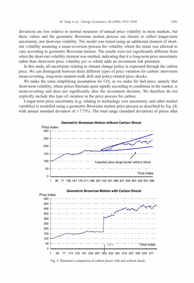
Longer-term price uncertainty (e.g. relating to technology cost uncertainty and other marketvariables) is modelled using a geometric Brownian motion price process as described by Eq. (4)with annual standard deviation of ±7.75%. The total range (standard deviation) of prices after

Fig. 4. Illustrative comparison of carbon prices with and without shock.

1942 M. Yang et al. / Energy Economics 30 (2008) 1933–1950

15 years would be ±30%. This is chosen to match the range of gas price uncertainty used in themodel. The expected mean carbon price is taken to be $25/tCO2 throughout the modelling period.

We have developed a special step function to simulate carbon price shock or climate changepolicy uncertainty in addition to its annual stochastic price variation. This represents an ‘informationevent’ or carbon price shock resulting from a policy announcement such as might arise at thebeginning of a new allocation period in an emissions trading scheme, or the announcement of a newregulatory intervention. The possible shock in carbon price due to such an event is assumed to occurin one particular year of the run τ. Prior to year τ, prices vary according to geometric Brownianmotion. The price in year τ has an additional randomised component representing the price shock.Prices in year τ+1 and beyond continue according to geometric Brownian motion starting fromthe new position after the shock. This means that the uncertainty associated with the price shock(representing policy uncertainty due to special event) is assumed to be resolved after year τ, so thatprices continue with some annual variability at the new level determined by the level of the priceshock. Our carbon price modelling was derived fromDixit and Pindyck (1994 p65) by adding a stepfunction ηx(2dy−1). See formula (5). We use xc to represent carbon price. Parameters α,σ dz are thesame as in Eq. (4). Parameter dy is a uniform random variable with a value between 0 and 1 designedto simulate the shock of carbon price at the particular event t=τ. The value of the step function is anadditional toWiener process of the carbon price variation at t=τ. The coefficientη defines the size ofthe price shock, and is typically set to a value of 1 in most runs. The term ηxc(2dy−1) thereforerepresents a price shock in the range ±100% (i.e., anywhere between a doubling of prices or acollapse of prices to near zero). The year in which the shock occurs can be varied — we compareresults where the shock occurs after 5 years versus a case where the shock occurs after 10 years.

dxc ¼axcdt þ rxcdzþ gxcð2dy� 1Þ; when t ¼ s

axcdt þ rxcdz; when t p s

8<: ð5Þ

Fig. 4 demonstrates the modelling effect of Eq. (5). It consists of two charts: Geometric BrownMotion without Carbon Shock and Geometric BrownMotion with Carbon Shock. The two curvesare identical if the step function (ηxt−1(2dy−1) is taken away. As indicated above, we assume theshock takes place at t=τ. The two lines starting at t=τ in the chart without shock form anexpected price range or area. However, if carbon price shock happens, the price range or area willlikely be completely changed. See the chart with carbon price shock.

The expected value of carbon in the model depends on the investment option being considered.The main aim of the modelling is to understand the effects of uncertainty, not whether a particularinvestment is cost-effective under any particular carbon price scenario. We therefore set carbonprices close to a level where the investment would be considered just financially viable under anormal NPV rule. We then introduce the stochastic price variations and run the model to find thenew optimal investment rule which can be compared with the NPV rule to provide an analysis ofthe effect of uncertainty on investment risk premiums.

Correlation between different stochastic variables can be introduced into the model byensuring that there is correlation in the selection of the randomisation elements dzi for the differentvariables i. The key correlation that needs to be considered is between gas prices and CO2 prices(since electricity prices in any case incorporate variability in these two inputs). It is plausible toassume that gas and CO2 prices will be partially correlated in an emissions trading schemebecause of the role of these prices in the dispatch decisions of power generators. When gas pricesare high, the generators will tend to prefer to dispatch coal-fired plant, thereby pushing up carbon

1943M. Yang et al. / Energy Economics 30 (2008) 1933–1950

prices. On the other hand, CO2 prices may respond to a whole range of other stimuli. In the runspresented here, we assume a moderate correlation coefficient of around 0.5.

Electricity prices are assumed to follow the short-run marginal costs (SRMC) of existing plantoperating at the margin of the electricity system. Three different assumptions are made about whattype of plant the SRMC is based on:

1. Coal-fired plants are always on the margin and entirely determine SRMC.2. Gas-fired plants are always on the margin and entirely determine SRMC.3. The marginal plant in the electricity system will be that which has the greatest SRMC, chosen

by the model (between a coal plant and a gas plant) depending on the outturn fuel and CO2 costsin any given year. In this case, it is assumed that there is a mix of existing coal and gas plants inthe system, so that 80% of the timemarginal demandwill bemet by the plant with higher SRMCfor that year, and 20% of the time marginal demand will be met by the plant with lower SRMCfor that year (i.e., during off-peak times). The merit order may change from one year to the nextduring the run depending on what happens to the stochastic CO2 and fuel prices.

In all three cases, the SRMC calculates fuel costs based on assumed plant efficiencies forexisting plant of 38% for a coal plant and 48% for a gas plant, fixed operating and maintenancecosts of $3.33/MWh for a coal plant and $1.5/MWh for a gas plant, and CO2 costs based onemissions factors of 94.6 tCO2/TJ input fuel for a coal plant and 56.1 tCO2/TJ input fuel for a gasplant. The final price of electricity comprises the SRMC element plus an additional spark spread1

of $5.5/MWh which is assumed to vary stochastically, according to geometric Brownian motionwith a 20% annual volatility, zero correlation with gas prices and moderate (37%) correlation withCO2 price variations. These assumptions about the price formation process for electricity arerelevant to competitive markets where electricity prices are determined by the cost of generation ofthemarginal plant in the system. In price-regulated markets, a firm's revenue will be determined bythe costs of generation of each individual plant in their fleet. This would lead to a different riskexposure.

2.6. Calculation of risk premiums

The risk premiums of climate policy uncertainty impact on power investment werecalculated under two scenarios. In the first scenario, we used the traditional project evaluationmethod, namely discounted cash flow without taking into account price uncertainty, ADB(2002). In this method, investment capital, project operation and maintenance costs, futurecarbon price, energy price and project revenue were all taken as non-stochastic, at theirexpected values, subject to deterministic rates of growth. With these certain values, wecalculated the project cash flow and discounted it to get the net present value (NPVcertain) of theproject. In the second scenario, we use the ROAwith carbon and energy prices set as uncertainvariables. The distribution of the project NPVuncertain including the option to optimise thetiming of the investment decision is derived by hundreds of thousands of Monte Carlosimulations. More details on the calculation of the NPV distribution and all other equations ofthe whole model can be found in Yang and Blyth (2007). By comparing the expected NPVs of

1 The spark spread is the nominal trading contribution of a gas-fired power plant from selling a unit of electricity,having bought the fuel required to produce (at 48% efficiency) this unit of electricity. All other power plant costs(operation and maintenance, capital and other financial costs) must be recovered from the spark spread.

1944 M. Yang et al. / Energy Economics 30 (2008) 1933–1950

the two scenarios, we derived the premium of carbon price, i.e., climate policy, uncertainty. Ina simplified mathematical equation, it can be expressed as follows:

RPðUSD=kWÞ ¼ ðNPVuncertain � NPVcertainÞðUSDÞCapacityðkWÞ ð6Þ

Where: RP (USD/kW) is the risk premium of the project investment, (NPVuncertain−NPVcertain) represents the additional revenue of the project in USD, which is required to triggerinvestment at year t, and the Capacity is the total additional capacity in kW due to the investment.

3. Scenarios, assumptions and technology data

To identify the relative importance of CO2 price uncertainty and fuel price uncertainty, themodel was run separately for three different scenarios: (1) keeping CO2 prices constant withstochastic fuel prices; (2) keeping fuel prices unchanged with CO2 prices changing randomly; and(3) with both CO2 and fuel prices varying stochastically. The model was also run with threedifferent assumptions about which type of plant would be on the margin of the system andtherefore setting electricity prices: (1) coal plants determine prices; (2) gas plants determineprices; and (3) the model determines the marginal plant (either coal or gas) depending on theprevailing fuel and CO2 prices in any year.

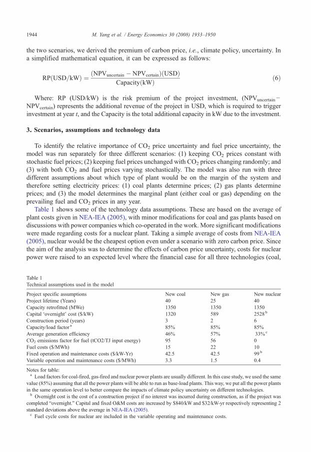
Table 1 shows some of the technology data assumptions. These are based on the average ofplant costs given in NEA-IEA (2005), with minor modifications for coal and gas plants based ondiscussions with power companies which co-operated in the work. More significant modificationswere made regarding costs for a nuclear plant. Taking a simple average of costs from NEA-IEA(2005), nuclear would be the cheapest option even under a scenario with zero carbon price. Sincethe aim of the analysis was to determine the effects of carbon price uncertainty, costs for nuclearpower were raised to an expected level where the financial case for all three technologies (coal,

Table 1Technical assumptions used in the model

Project specific assumptions New coal New gas New nuclearProject lifetime (Years) 40 25 40Capacity retrofitted (MWe) 1350 1350 1350Capital ‘overnight’ cost ($/kW) 1320 589 2528 b

Construction period (years) 3 2 6Capacity/load factor a 85% 85% 85%Average generation efficiency 46% 57% 33%c

CO2 emissions factor for fuel (tCO2/TJ input energy) 95 56 0Fuel costs ($/MWh) 15 22 10Fixed operation and maintenance costs ($/kW-Yr) 42.5 42.5 99 b

Variable operation and maintenance costs ($/MWh) 3.3 1.5 0.4

Notes for table:a Load factors for coal-fired, gas-fired and nuclear power plants are usually different. In this case study, we used the same

value (85%) assuming that all the power plants will be able to run as base-load plants. This way, we put all the power plantsin the same operation level to better compare the impacts of climate policy uncertainty on different technologies.b Overnight cost is the cost of a construction project if no interest was incurred during construction, as if the project was

completed “overnight.” Capital and fixed O&M costs are increased by $840/kW and $32/kW-yr respectively representing 2standard deviations above the average in NEA-IEA (2005).c Fuel cycle costs for nuclear are included in the variable operating and maintenance costs.

1945M. Yang et al. / Energy Economics 30 (2008) 1933–1950

gas and nuclear) were approximately equivalent under our fuel and CO2 price assumptions.Although this meant raising capital and operating costs for nuclear power by two standarddeviations relative to the mean in NEA-IEA (2005), these figures are still lower than other recentestimates used for policy analysis purposes (e.g. DTI, 2006).

The technology data includes assumptions about the build time for each technology. This istaken to be the delay between committing capital to the project and generating revenue. Capital isassumed to be spent at a constant rate over this period. The discount rate used throughout for thecash-flow for evaluating present values of future costs and revenues is 7%. Capital costs areassumed to be subject to an annual depreciation tax shield of 13.3% of capital costs against acorporation tax rate of 31%. Final cash-flows and risk premiums are evaluated post tax.

In this study, we did not explicitly consider technical risks. The capital and operating costs ofeach technology, as well as their performance characteristics (efficiency, load factor, etc.) wereassumed to be known with certainty. In principle however, the methodology described in thispaper could be extended to analyse the effects of these important additional sources of risk.

4. Results

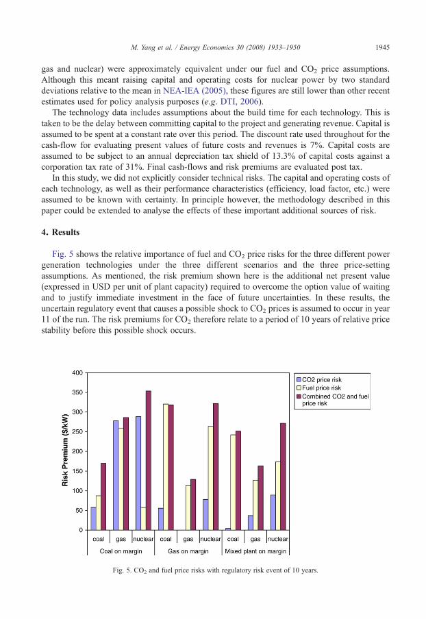
Fig. 5 shows the relative importance of fuel and CO2 price risks for the three different powergeneration technologies under the three different scenarios and the three price-settingassumptions. As mentioned, the risk premium shown here is the additional net present value(expressed in USD per unit of plant capacity) required to overcome the option value of waitingand to justify immediate investment in the face of future uncertainties. In these results, theuncertain regulatory event that causes a possible shock to CO2 prices is assumed to occur in year11 of the run. The risk premiums for CO2 therefore relate to a period of 10 years of relative pricestability before this possible shock occurs.

Fig. 5. CO2 and fuel price risks with regulatory risk event of 10 years.

1946 M. Yang et al. / Energy Economics 30 (2008) 1933–1950

4.1. CO2 price risk

In most of the cases shown in Fig. 5, CO2 price risk is not very significant. The exceptions arefor gas and nuclear plants when a coal plant is on the margin. If a coal plant is at the margin of themerit order (see the left-hand block of the results in Fig. 5), CO2 prices are assumed to be passedthrough to electricity prices at a rate determined by the high emission levels of a coal plant. Gas andnuclear power investments would in this case be strongly affected by changes in CO2 price. This isnot the case for a coal plant, since changes in CO2 price would affect both costs and revenues by asimilar amount, leaving overall profitability relatively insensitive to changes in CO2 price.

When a gas plant is on the margin (see the central block of results in Fig. 5), the rate of feed-through of CO2 prices to electricity prices is significantly lower because of the lower emissionlevels of a combined cycle gas turbine (CCGT) plant compared to a coal plant. Therefore the CO2

price risk for coal and nuclear plants is quite low.When the marginal plant is allowed to vary (i.e., “mixed plant on margin” results on the right of

Fig. 5), CO2 price risk is still quite low, as this case is actually closer to the 100% gas plant on themargin case than the 100% coal plant on the margin case under the assumptions made in the model.

4.2. Fuel price risk

Coal prices are assumed in the model to be relatively stable, so fuel price risk is mostly createdby uncertainty in gas price, and the possibility for this to feed through to the electricity price. Inthe case where a coal plant is always on the margin, the electricity price is unaffected by gas priceuncertainty, so the fuel price risk for coal and nuclear plants is low. The fuel price risk for a gasplant in this case is high because gas price fluctuations would affect the generation costs withoutany corresponding change in the revenues.

In the case where a gas plant is always on the margin however, the fuel price risks for a new gasplant are low because fluctuations in fuel prices would show up in corresponding fluctuations inthe revenue, leaving overall profitability relatively insensitive to fuel price changes. Coal andnuclear plants would be heavily exposed in this case to gas price fluctuations via the feed-throughof these fluctuations to the electricity price.

The fuel price risk is reduced slightly in the case with mixed plant on the margin because forsome fraction of the time a coal plant would be setting the electricity price, thereby reducing onaverage the expected level of price fluctuations.

4.3. Combined CO2 and fuel price uncertainty

The combined risk is not a simple addition of the fuel and CO2 price risks, since it has to takeaccount of the correlation between the two sets of prices. An interesting example is to compare gaspower and nuclear power investments under the “coal onmargin” case. The nuclear plant investmenthas high CO2 price risk but low fuel price risk, giving a combined risk premium only slightly greaterthan the CO2 price risk premium. The gas power investment has high CO2 risks and high fuel pricerisks, but the combined total is not much higher than the sum of the individual components. Thereason is that there is assumed to be some correlation between gas prices and CO2 prices. Therefore,when gas prices are lower than expected (favouring the investment in a gas plant), the CO2 priceswillalso tend to be lower than expected, offsetting some of the benefits of the low gas price.

In any case, it is interesting to note that in all three cases of different assumptions of themarginal plant, nuclear power investments appear to be amongst the most risky. The reason is that

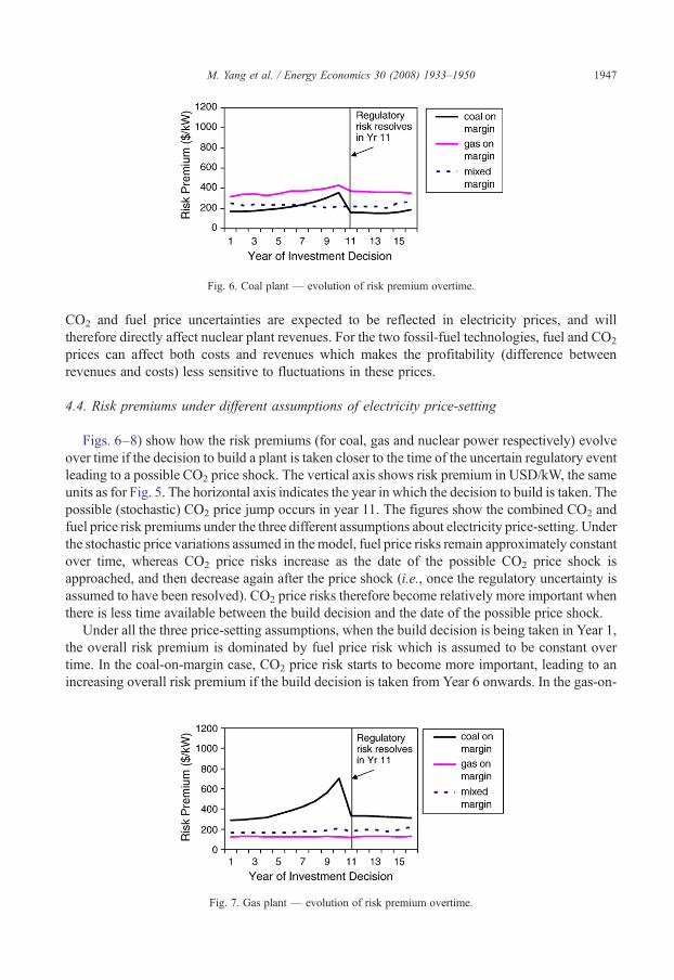
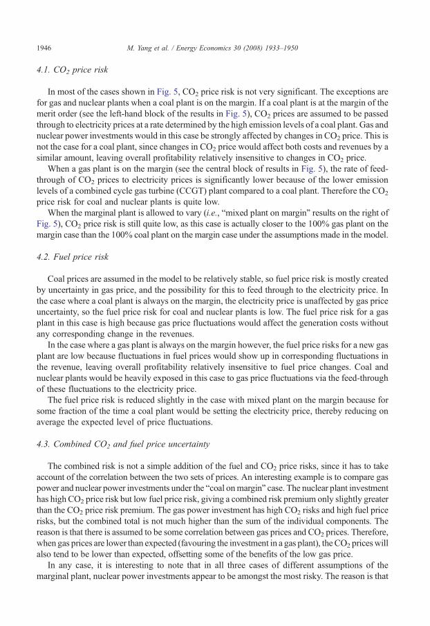
Fig. 6. Coal plant — evolution of risk premium overtime.

1947M. Yang et al. / Energy Economics 30 (2008) 1933–1950

CO2 and fuel price uncertainties are expected to be reflected in electricity prices, and willtherefore directly affect nuclear plant revenues. For the two fossil-fuel technologies, fuel and CO2

prices can affect both costs and revenues which makes the profitability (difference betweenrevenues and costs) less sensitive to fluctuations in these prices.

4.4. Risk premiums under different assumptions of electricity price-setting

Figs. 6–8) show how the risk premiums (for coal, gas and nuclear power respectively) evolveover time if the decision to build a plant is taken closer to the time of the uncertain regulatory eventleading to a possible CO2 price shock. The vertical axis shows risk premium in USD/kW, the sameunits as for Fig. 5. The horizontal axis indicates the year in which the decision to build is taken. Thepossible (stochastic) CO2 price jump occurs in year 11. The figures show the combined CO2 andfuel price risk premiums under the three different assumptions about electricity price-setting. Underthe stochastic price variations assumed in the model, fuel price risks remain approximately constantover time, whereas CO2 price risks increase as the date of the possible CO2 price shock isapproached, and then decrease again after the price shock (i.e., once the regulatory uncertainty isassumed to have been resolved). CO2 price risks therefore become relatively more important whenthere is less time available between the build decision and the date of the possible price shock.

Under all the three price-setting assumptions, when the build decision is being taken in Year 1,the overall risk premium is dominated by fuel price risk which is assumed to be constant overtime. In the coal-on-margin case, CO2 price risk starts to become more important, leading to anincreasing overall risk premium if the build decision is taken from Year 6 onwards. In the gas-on-

Fig. 7. Gas plant — evolution of risk premium overtime.

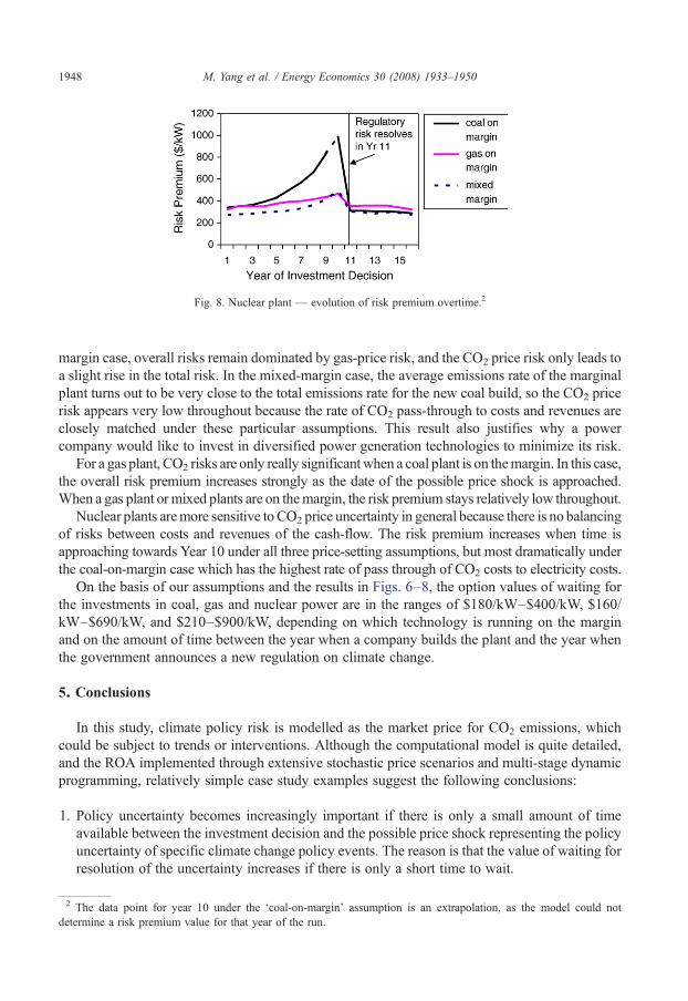
Fig. 8. Nuclear plant — evolution of risk premium overtime.2

1948 M. Yang et al. / Energy Economics 30 (2008) 1933–1950

margin case, overall risks remain dominated by gas-price risk, and the CO2 price risk only leads toa slight rise in the total risk. In the mixed-margin case, the average emissions rate of the marginalplant turns out to be very close to the total emissions rate for the new coal build, so the CO2 pricerisk appears very low throughout because the rate of CO2 pass-through to costs and revenues areclosely matched under these particular assumptions. This result also justifies why a powercompany would like to invest in diversified power generation technologies to minimize its risk.

For a gas plant, CO2 risks are only really significant when a coal plant is on themargin. In this case,the overall risk premium increases strongly as the date of the possible price shock is approached.When a gas plant or mixed plants are on themargin, the risk premium stays relatively low throughout.

Nuclear plants aremore sensitive to CO2 price uncertainty in general because there is no balancingof risks between costs and revenues of the cash-flow. The risk premium increases when time isapproaching towards Year 10 under all three price-setting assumptions, but most dramatically underthe coal-on-margin case which has the highest rate of pass through of CO2 costs to electricity costs.

On the basis of our assumptions and the results in Figs. 6–8, the option values of waiting forthe investments in coal, gas and nuclear power are in the ranges of $180/kW–$400/kW, $160/kW–$690/kW, and $210–$900/kW, depending on which technology is running on the marginand on the amount of time between the year when a company builds the plant and the year whenthe government announces a new regulation on climate change.

5. Conclusions

In this study, climate policy risk is modelled as the market price for CO2 emissions, whichcould be subject to trends or interventions. Although the computational model is quite detailed,and the ROA implemented through extensive stochastic price scenarios and multi-stage dynamicprogramming, relatively simple case study examples suggest the following conclusions:

1. Policy uncertainty becomes increasingly important if there is only a small amount of timeavailable between the investment decision and the possible price shock representing the policyuncertainty of specific climate change policy events. The reason is that the value of waiting forresolution of the uncertainty increases if there is only a short time to wait.

2 The data point for year 10 under the ‘coal-on-margin’ assumption is an extrapolation, as the model could notdetermine a risk premium value for that year of the run.

1949M. Yang et al. / Energy Economics 30 (2008) 1933–1950

2. The risk premium created by policy uncertainty depends on how the uncertainty feeds throughto electricity prices. CO2 price risks will generally be more important if electricity pricesfollow the generation costs of a coal plant, as these will pass through CO2 costs (and thereforecost uncertainties) at a higher rate.

3. Nuclear plants appear to be the most exposed to CO2 and fuel price risks of the threetechnologies investigated. For investments of a coal plant and a gas plant, variations in theprice of CO2 and fuel affect both costs and revenues, thus dampening the effect of thesevariations on profitability. Nuclear plants are nevertheless exposed to the full revenue risk,with no offsetting through the variability in costs.

These conclusions depend on a number of key assumptions. Firstly, the electricity priceformation process is crucial. This study is relevant to a situation where electricity prices are set ina competitive market, assuming that prices are determined by the cost of generation of themarginal plant in the system, and that all other power plants are price takers. In an alternativesituation where revenues are based on regulated prices, a firm may instead receive revenuesrelated to the actual costs that individual power plants incur. In this situation, the investment risksto the firm may be very much lower than those indicated in this paper, and a nuclear power plantin particular may face less commercial risk.

A second important assumption is that all policy risk is represented through the CO2 priceuncertainty. This is a convenient surrogate for analytical purposes. However, in emissions tradingmarkets where there is free allocation, there will be additional uncertainty relating to the level ofthis free allocation, which effectively acts as a transfer of assets between the issuer of allowances(i.e. government) and the generators. The rules over allocation to fossil-fuel generators cancertainly influence the choice of generation technology. In particular, free allocation to newentrants acts as a subsidy to fossil-fuel generators. Uncertainty in these rules can be an additionalsource of regulatory risk that has not been addressed in this paper, although the methodologydescribed could be extended to consider this source of risk.

Finally, the paper did not consider technical risks such as uncertain costs, performance or loadfactor. The purpose of the study was to investigate the magnitude and effects of regulatory risk,and the authors did not aim to provide a full risk analysis of different investment options.Nevertheless, the real options methodology described here could be extended to include theseimportant sources of risk, and this could be a fruitful area of further work.

The overall conclusion of this work is that the quantitative valuation of policy risk can add animportant dimension to the analysis of climate change policy because of the potentially significantincremental effect of risk on incentives for investment. Risk premiums calculated in theillustrative examples were in some cases a substantial proportion of the capital costs of theinvestment, and could be sufficient to tilt investment choice away from those suggested by simpledeterministic and expected NPV analyses.

Acknowledgements

The authors acknowledge the support for this work from the governments of Canada,Netherlands and the UK, as well as from Enel, E.ON-UK, EPRI and RWE-npower.Acknowledgement is due to the Prof. Richard Tol, the editor of Energy Economics, and twoanonymous reviewers for their time and valuable comments on the manuscript. For more detailedinformation on this ROA study, please see IEA (2007): “Climate Policy Uncertainty and InvestmentRisk” at http://www.iea.org/w/bookshop/add.aspx?id=305 or www.iea.org/books.

1950 M. Yang et al. / Energy Economics 30 (2008) 1933–1950

References

ADB (Asian Development Bank), 2002. Guidelines for the Financial Governance and Management of Investment ProjectsFinanced by the Asian Development Bank. Asian Development Bank, Manila, Philippines. January.

Dixit, A.K., Pindyck, R.S., 1994. Investment under Uncertainty. Princeton University Press, Princeton, USA. ISBN: 0-691-03410-9.

DTI (Department of Trade & Industry of the UK), 2006. The Energy Challenge. Energy Review, London. July.EPRI (Electric Power Research Institute), 1999. A Framework for Hedging the Risk of Greenhouse Gas Regulations. Palo

Alto, CA, USA: TR-113642.IEA (International Energy Agency), 2004. World Energy Outlook. Paris, France. ISBN: 92-64-10817-3.IEA (International Energy Agency), 2007. Climate Policy Uncertainty and Investment Risk. Paris France. ISBN: 978-92-

64-03014-5. April.Kuper, G.H., Soest, D.P., 2006. Does oil price uncertainty affect energy use? Energy Journal 27 (1), 55–78.Laughton, D., Hyndman, R., Weaver, A., Gillett, N., Webster, M., Allen, M., Koehler, J., 2003. A Real Options Analysis of

a GHG Sequestration Project. The paper is available from David Laughton at: david.laughton@ualberta.ca.Laurikka, H., 2006. Option value of gasification technology within an emissions trading scheme. Energy Policy 34 (18),

3916–3928. December.Lin, T.T., Ko, C.C., Yeh, H.N., 2007. Applying real options in investment decisions relating to environmental pollution.

Energy Policy 35, 2426–2432.Marreco, J.M., Carpio, L.G.T., 2006. Flexibility valuation in the Brazilian power system — a real options approach.

Energy Policy 34 (18), 3749–3756.Myers, S.C., 1977. The determinants of corporate borrowing. Journal of Financial Economics 5, 147–175.NEA-IEA (NEA: Nuclear Energy Agency of the OECD), 2005. Projected Costs of Generating Electricity. OECD, Paris.Rothwell, G.A., 2006. A real options approach to evaluating new nuclear power plants. The Energy Journal 27 (1), 37–53.Sekar, C., 2005. Carbon Dioxide Capture from Coal-Fired Power Plants: A Real Options Analysis. Massachusetts Institute

of Technology, Laboratory for Energy and the Environment, 77 Massachusetts Avenue, Cambridge, MA 02139-4307,USA.

Siddiqui, A.S., Marnay, C., Wiser, R.H., 2007. Real options valuation of US Federal Renewable Energy Research,development, demonstration, and development. Energy Policy 35 (1), 265–279 (January).

Yang, M., Blyth, W., 2007. Modeling investment risks and uncertainties with real options approach. International EnergyAgency Working Paper Series LTO/2007/WP 01, Paris.