Embed Size (px)
Citation preview
GEOMETRY TEACHER'S EDITION
Exploring Centers
HENRY KRANENDONK AND JEFFREY WITMER
DATA-DRIVEN MATHEMATICS
D A L E S E Y M 0 U R P U B L I C A T I 0 N S®
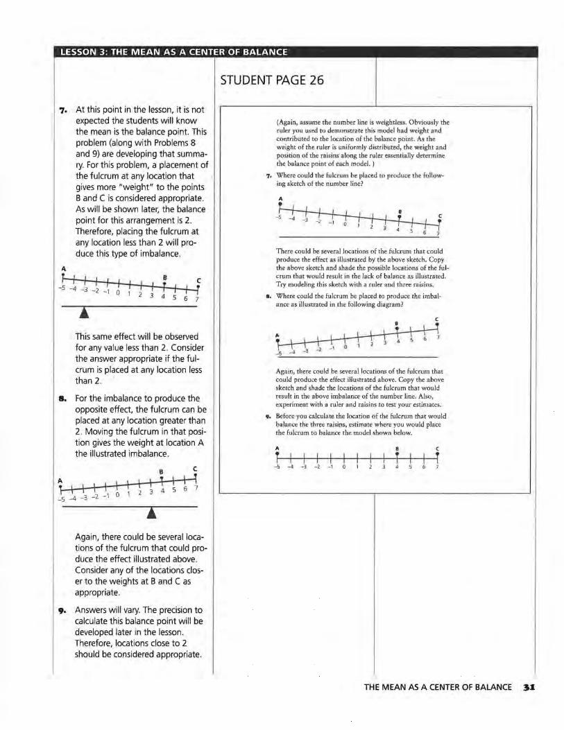
Exploring Centers
TEACHER'S EDITION
DATA-DRIVEN MATHEMATICS
Henry Kranendonk and Jeffrey Witmer
Dale Seymour Publications® Orangeburg, New York
This material was produced as a part of the American Statistical Association's Project "A Data-Driven Curriculum Strand for High School" with funding through the National Science Foundation, Grant #MDR-9054648. Any opinions, findings, conclusions, or recommendations expressed in this publication are those of the authors and do not necessarily reflect the views of the National Science Foundation.
This book is published by Dale Seymour Publications®, an imprint of Addison Wesley Longman, Inc.
Dale Seymour Publications 125 Greenbush Road South Orangeburg, NY 10962 Customer Service: 800-872-1100
Copyright© 1998 by Dale Seymour Publications®. All rights reserved. No part of this publication may be reproduced in any form or by any means without the prior written permission of the publisher.
Printed in the United States of America.
Order number DS21177
ISBN 1-57232-236-5
1 2 3 4 5 6 7 8 9 10-ML-02 01 00 99 98 97
This Book ls Printed On Recycled Paper
CALE SEYMOUR PUBLICATIONS®
Managing Editor: Cathy Anderson
Senior Math Editor: Carol Zacny
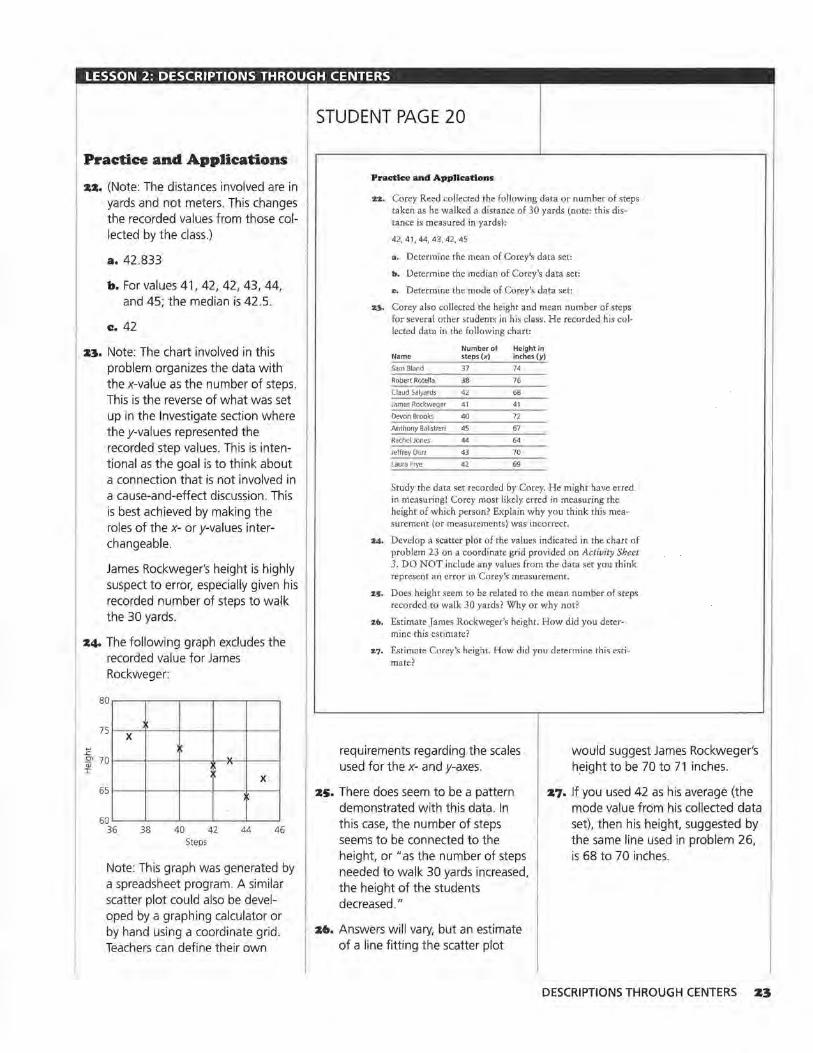
Consulting Editor: Maureen Laude
Production/Manufacturing Director: Janet Yearian
Senior Production Coordinator: Alan Noyes
Design Manager: Jeff Kelly
Text and Cover Design: Christy Butterfield
Cover Photograph: Stuart Hunter/Masterfile
Authors
Henry Kranendonk Rufus King High School Milwaukee, Wisconsin
.Jeffrey Witmer Oberlin College Oberlin, Ohio
Consultants
Jack Burrill Whitnall High School Greenfield, Wisconsin University of Wisconsin-Madison Madison, Wisconsin
Vince O'Connor Milwaukee Public Schools Milwaukee, Wisconsin
Emily Errthum Homestead High School Mequon, Wisconsin
Maria Mastromatteo Brown Middle School Ravenna, Ohio
Oata-Ori11en ll/lalllematlcs Leadership Team
Miriam Clifford Nicolet High School Glendale, Wisconsin
James M. Landwehr Bell Laboratories Lucent Technologies Murray Hill, New Jersey
Kenneth Sherrick Berlin High School Berlin, Connecticut
Gail F. Burrill Whitnall High School Greenfield, Wisconsin University of Wisconsin-Madison Madison, Wisconsin
Patrick Hopfensperger Homestead High School Mequon, Wisconsin
Richard Scheaffer University of Florida Gainesville, Florida
Acknowledgments
The authors thank the following people for their assistance during the preparation of this module:
The many teachers who reviewed drafts and participated in fields tests of the manuscripts
Sharon Hemet for working through the material with her students
Michelle Fitzgerald for working through the material with her students
Elizabeth Radtke for working through the material with her students
Ron Moreland and Peggy Layton for their advice and suggestions in the early stages of the writing
The many students from Washington High School and Rufus King High School who helped shape the ideas as they were being developed.
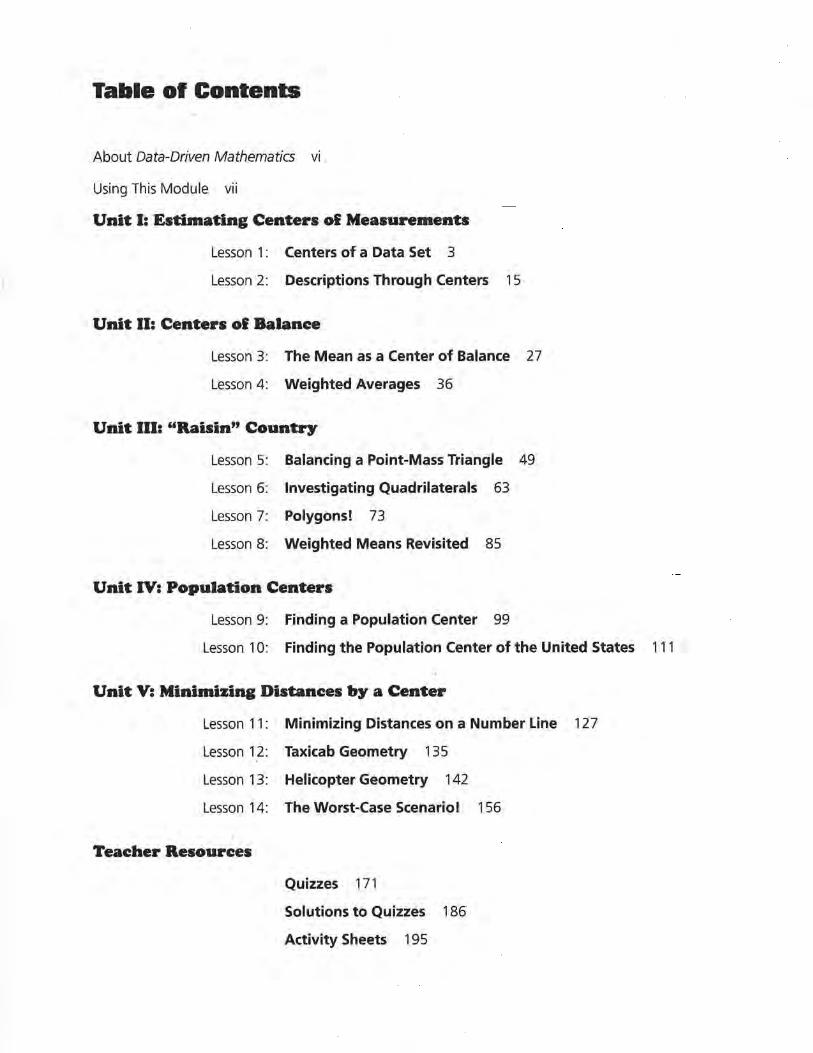
Table of Contents
About Data-Driven Mathematics vi
Using This Module vii
Unit I: Estimating Centers of Measurements
Lesson 1 : Centers of a Data Set 3
Lesson 2: Descriptions Through Centers 15
Unit II: Centers of Balance
Lesson 3: The Mean as a Center of Balance 27
Lesson 4: Weighted Averages 36
Unit Ill: "Raisin" Country
Lesson 5: Balancing a Point-Mass Triangle 49
Lesson 6: Investigating Quadrilaterals 63
Lesson 7: Polygons! 73
Lesson 8: Weighted Means Revisited 85
Unit IV: Population Centers
Lesson 9: Finding a Population Center 99
Lesson 10: Finding the Population Center of the United States 111
Unit V: Minimizing Distances by a Center
Lesson 11: Minimizing Distances on a Number Line 127
Lesson 12: Taxicab Geometry 135
Lesson 13: Helicopter Geometry 142
Lesson 14: The Worst-Case Scenario! 156
Teacher Resources
Quizzes 171
Solutions to Quizzes 186
Activity Sheets 195
About Oata-Oriven Malllematics
Historically, the purposes of secondary-school mathematics have been to provide students with opportunities to acquire the mathematical knowledge needed for daily life and effective citizenship, to prepare students for the workforce, and to prepare students for postsecondary education. In order to accomplish these purposes today, students must be able to analyze, interpret, and communicate information from data.
Data-Driven Mathematics is a series of modules meant to complement a mathematics curriculum in the process of reform. The modules offer materials that integrate data analysis with high-school mathematics courses. Using these materials will help teachers motivate, develop, and reinforce concepts taught in current texts. The materials incorporate the major concepts from data analysis to provide realistic situations for the development of mathematical knowledge and realistic opportunities for practice. The extensive use of real data provides opportunities for students to engage in meaningful mathematics. The use of real-world examples increases student motivation and provides opportunities to apply the mathematics taught in secondary school.
The project, funded by the National Science Foundation, included writing and field-testing the modules, and holding conferences for teachers to introduce them to the materials and to seek their input on the form and direction of the modules. The modules are the result of a collaboration between statisticians and teachers who have agreed on the statistical concepts most important for students to know and the relationship of these concepts to the secondary mathematics curriculum.
A diagram of the modules and possible relationships to the curriculum is on the back cover of each Teacher's Edition.
vi ABOUT DATA-DRIVEN MATHEMATICS
Using This Module
Exploring Centers is designed to integrate mathematical and statistical topics within a geometry class for high school students. The primary goal is to use measurements, shapes, distances, and principles of balance as a way to explore problems working with centers. Centers will initially strike students as merely a study of circles since their primary connection with this word is within that context. This module is designed to expand students' perspective of centers and to demonstrate that centers is a concept with a variety of interpretations and applications. Although the relationship to a circle is presented in the latter sections of this module, centers are also developed as numerical summaries of data, locations to balance weights, points or locations to equalize directed distances, locations to combine the impact of distance and weight, locations to minimize distances, or locations or points to minimize extremes. A center represents an attempt to be fair and to equalize the parameters important in special problems. For these reasons, a center is not an easy term to define. The use of the word becomes related to the specific problems investigated by the student. This module attempts to investigate several problems that are interesting and significant because of the connections to a center.
Why the Content Is Important
The mathematics incorporated in this module primarily involves using appropriate methods for summarizing data for generalizations and decision making. Several of the lessons require students to collect data; other lessons present data sets used by students to complete the problems. In all cases, the lessons guide students into organizing data, developing summaries (for example, the mean), and interpreting the results as directed by the larger questions or investigations. This process encourages students to investigate new types of problems and questions.
The mathematics used in the lessons is especially important because it enables students to understand the questions presented. Although many of the questions do not directly ask a mathematical question, students need to apply various mathematical topics to develop their solutions. The topics outlined in the Mathematical Content and Statistical Content become for students the tools in making decisions and explaining their solutions.
Mathematical Content
• Signed number operations
• Representation and interpretation of numbers on a number line
• Coordinate geometry applications: Plotting points on a coordinate grid Interpreting points from a coordinate system Constructing coordinate systems
USING THIS MODULE vii
• Mathematical formulas
• Calculation of distances on a number line or coordinate grid
Statistical Content
• Calculation and interpretation of summary statistics
• Symbolic expressions for statistical summaries
• Interpretation of means as related to weight and distance
• Interpretation of medians
• Relationship of summary statistics to the interpretation of an application
Teacher Resources
At the back of this Teacher's Edition are the following:
• Quizzes • Solution Key for quizzes
• Activity Sheets
viii USING THIS MODULE
Use oi Teacher Resources
These items are referenced in the Materials section at the beginning of each lesson.
LESSONS RESOURCE MATERIALS
Lesson 1 : Problem 1 Sa • Activity Sheet 1: Data Summary 1 (for scale drawing)
Lesson 2: Problem 16 • Activity Sheet 2: Data Summary 2 (for "walking" activity)
Problems 19 and 24 • Activity Sheet 3: xy-coordinate Grid 1 Unit I Quiz
Lesson 4 • Unit II Quiz
Lesson 5 • Activity Sheet 4: Triangle Options • Activity Sheet 7: xy-coordinate Grid 2
Lesson 6 • Activity Sheet 5: Quadrilateral Options • Activity Sheet 7: xy-coordinate Grid 2
Lesson 7 • Activity Sheet 6: Pentagon Model •Activity Sheet 7: xy-coordinate Grid 2
Lesson 8 • Activity Sheet 6: Pentagon Model
• Activity Sheet 7: xy-coordinate Grid 2 • Unit Ill Quiz
Lesson 10 • Activity Sheet 8: U.S. Map (without coordinates) "The Big Picture " Project- • Activity Sheet 9: U.S. Map (with coordinates and state capitals) Options 2 and 3 • Activity Sheet 1 O: Data for U.S. Center Project
(A-without coordinates) • Activity Sheet 11: Data for U.S. Center Project
(B-with coordinates) •Activity Sheet 12: Summary of U.S. Center of Population • Unit IV Quiz
Lesson 12 • Activity Sheet 13: 3 x 3 and 5 x 5 Grids for Stores
Lesson 13 • Activity Sheet 13: 3 x 3 and 5 x 5 Grids for Stores
Lesson 14 • Activity Sheet 13: 3 x 3 and 5 x 5 Grids for Stores • Unit V Quiz
USING THIS MODULE ix
Where to Use the Module in the Curriculum
This module is designed for use primarily within a geometry class or within a mathematics class incorporating the study of shapes and plane geometry topics. The lessons are developed to provide interest in statistical problems involving data sets collected and generated from geometric shapes and related topics in a geometric investigation.
This module includes five units. Each unit contains two to four lessons. The Pacing/Planning Guide indicates that several of the lessons ideally fit at the beginning of a typical geometry class, while other lessons should be used after preliminary work with geometric topics has been developed. This module can be used throughout an academic year in which larger investigations involving data and geometric inquiries would enhance the course.
Prerequisites
Students should have worked with signed number operations and general measurement problems before starting this module. Other sections require previous work with triangles, quadrilaterals, and other polygonal shapes. The detail of the prerequisite work with shapes is not extensive and should be covered in most 9th- or 10th-grade geometry classes. Some of the problems and investigations are quite involved and tedious. Group work is especially effective for those problems. As expected, however, completion of the tasks for these problems is dependent on students' willingness to work together in small groups.
Pacing/Planning Guide
The 14 lessons included in this module can be completed at various times in a geometry course or in a similar mathematics course. Most lessons are designed to be completed in 2 or 3 class sessions. The prerequisite skills described in the following table are general descriptions of the most important skills expected of students at the beginning of the unit. As indicated in the table, some of the lessons assume that identification and classification of geometric shapes have been previously learned by students. Also, some lessons assume familiarity with important characteristics of common shapes so that investigations and problems are more manageable. (For example, familiarity with the medians of a triangle or the diagonals of a parallelogram are important in Unit III. This is included in the Unit III summary.) Several skills not listed in this table are necessary in the lessons; however, they are developed as part of the objectives of the lessons and are not considered prerequisites.
x USING THIS MODULE
Pacing/Planning Guide
The table below provides a possible sequence and pacing of the units.
UNIT PREREQUISITE PACING TIMETABLE SKILLS (number of
class sessions)
Unit I: Estimating • Measuring distances with a ruler (2 lessons) Beginning of a Centers of • Operational skills with signed a total of 3 to geometry class Measurements numbers 4 sessions
Unit II: • Plotting and interpreting points on (2 lessons) Beginning of a Centers of a number line a total of geometry class Balance • Operational skills with signed numbers 4 sessions
Unit Ill: • Identification of angle and side (4 lessons) Middle of a geometry "Raisin" descriptions of triangles a total of 6 to class after prerequisite Country • Identification of the definition of 8 sessions skills have been
medians of a triangle developed through • Identification of polygons by the work with triangles,
number of sides and descriptions . quadrilaterals, and involving parallel lines, supplementary polygons angles, diagonals, and corresponding angles
• Plotting and interpreting points in a coordinate system
Unit IV: • Prerequisites similar to those of (2 lessons) Middle of a geometry Population Unit Ill a total of 4 to class Centers 6 sessions
(Lesson 10 Use right after Unit Ill involves a since several references project.) to examples and
illustrations in Lessons 5-8 are incorporated.
Unit V: Minimizing • Identification of terms related (4 lessons) Middle to end of a Distances by a to circles a total of 6 to geometry class; Center • Plotting and interpreting points 8 sessions recommended after
in a coordinate system general work with circles has been developed
USING THIS MODULE Jd
Technology
A graphing calculator similar to a TI-83 is needed for most of the lessons. Several of the lessons, particularly beginning with Unit III, would be well-supported with spreadsheet software. The calculator must have List capability. The linked cells of a spreadsheet offer a number of options in working with the data.
An overhead projector will be helpful. Overhead transparencies of particular data sets, graphs, or Activity Sheets can be useful during class discussion.
Grade Level/Course
This module is intended for a 9th- or 10th-grade geometry course or for a mathematics course involving investigations of geometric shapes. Although this module was designed to complement the geometry curriculum, it is also appropriate to use in a variety of courses designed to develop projects and work with data.
xii USING THIS MODULE
UNIT I
Estilnating Centers of
Measure1nents

LESSON 1
.Centers ol a Data Set Materials: tape measures and/or meter sticks, Activity Sheet 1 Technology: graphing calculator Pacing: 2 class sessions
Overview
Lesson 1 quickly introduces students to the data summaries of mean, median, and mode. This introduction assumes students are aware of these terms and might have previously worked with them. Mean, median, and mode are not introduced as centers but rather as possible data summaries that might qualify as a measure of center. This is an important point as the concept of a center is embedded in the nature of the particular problem.
This lesson develops an activity carried out by a geometry class at Rufus King High School and uses the data collected by the students. Each data set collected requires a summary in order to develop a scale drawing. The steps to implement this activity are outlined to help your students organize a similar investigation at your school site. This outline is provided in the student's lesson.
Teaching Notes
This lesson uses the familiar terms of mean, median, and mode to describe the collected data. Mean and median are the primary topics; however, a useful application of the mode is suggested. Emphasis of the mean and median is important since the primary applications of center in the lessons that follow are applications of these descriptions of centers.
This lesson does not conclude with a precise definition of center. This observation is intentional as the lesson is designed to encourage further investigations
in other lessons and modules of this series. A need for creating a center is based on the importance of communicating a summary of a collected set of data. This first lesson bases the importance of a center by using measurements and the variance of estimates resulting from this process.
Technology
As indicated, a scientific or graphing calculator is important to complete the numerous and often tedious calculations of the group activities. The type of calculator is not critical in this lesson; however, the List options of a calculator similar to a TI-82 or TI-83 could be applied to several problems. The format for using.the lists is suggested by the organization of the data sets in columns. This option, however, is not required and therefore is not highlighted in the lesson.
Follow-Up
A suggested follow-up for this lesson is outlined in the Further Practice section of this lesson. The field-test groups particularly enjoyed this extension and developed several small-group activities to highlight the local application of this lesson. This moved the lesson from the Rufus King High School model to the local school.
CENTERS OF A DATA SET ~
LESSON 1: CENTERS OF A DATA SET
STUDENT PAGE 3
4 LESSON 1
LESSON 1
Centers ol a Data Set
What is meant by a "center"?
How is a "center" calculated and interpreted?
The number representing your grade point average is a center, as well as the average number of students in a class or the average number of students arriving late to school. Would you consider the location of your locker as "centrally" located?
How would you determine this central location provided that was an important concern?
A lthough several examples of centers will be defined as these lessons are developed, examples based on the best
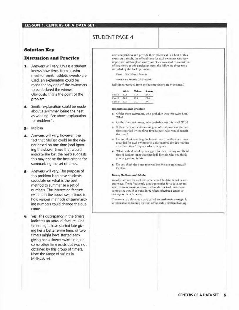
estimate of a set of data will start the discussion of centers. The importance of this type of center is demonstrated using the backup times collected at a swim meet. Whenever possible, an electronic clock is used to record a swimmer's official time. If, however, this clock does not function correctly, which can easily happen due to equipment problems or a poor "touch" by the swimmer, three backup timers are used. Surprisingly, it is rare to have the same times reported by the three backup timers. If three backup times are used, how do you think the official time is determined for a swimmer?
INVESTIGATE
Swim Meets
At a regional swim meet, Kristin, Melissa, and Shauna were involved in the same heat of the 50-yard freestyle. The top swimmers from each heat moved to the next level of competition. Their official times were used to both qualify them for the
Calculate the mean, median, and mode of
a data set.
Interpret a center as an estimation of a data set.
Visualize the accumulation of error
resulting from estimates of measured data.
LESSON 1: CENTERS OF A DATA SET
Solution Key
Discussion and Practice
1. Answers will vary. Unless a student knows how times from a swim meet (or similar athletic events) are used, an explanation could be made for any one of the swimmers to be declared the winner. Obviously, this is the point of the problem.
z. Similar explanation could be made about a swimmer losing the heat as winning. See above explanation for problem 1 .
:J. Melissa
4. Answers will vary, however, the fact that Melissa could be the win-ner based on one time (and ignor-ing the slower times that would indicate she lost the heat) suggests this may not be the best criteria for summarizing the set of times.
s. Answers will vary. The purpose of this problem is to have students speculate on what is the best method to summarize a set of numbers. The interesting feature evident in the above swim times is how various methods of summariz-ing numbers could change the out-come.
6. Yes. The discrepancy in the timers indicates an unusual feature. One timer might have started late giv-ing her a better swim time, or two timers might have started early giving her a slower swim time, or some other time exists but was not obtained by this group of timers. Note the range of values in Melissa's set.
STUDENT PAGE 4
next competition and provide their placement in a heat of this event. As a result, the official time for each swimmer was very important! Although an electronic clock was used to record the official times at this particular meet, the following times were recorded by the backup timers:
Event: Girls' SO-yard Freestyle
Swim Club Record: 27 ,0 seconds
(All times recorded from the backup timers are in seconds.)
Kristin Melissa Shauna
Timer 1 27,2 27 4 27 3
Timer 2 27.3 27 4 27 4
Timer 3 27~ 1 27.0 27. 1
Discussion and Practice
1. Of the three swimmers, who probably won this swim heat? Why?
z. Of the three swimmers, who probably lost this heat? Why?
3. If the criterion for determining an official time was the best time recorded by the three timekeepers, who would benefit the most?
4, Do you think selecting the fastest time from the three times recorded for each swimmer is a fair method for determining an official time? Explain why or why not.
5. What method would you suggest for determining an official time if backup times were needed? Explain why you think your suggestion i.s fair.,
c.. Do you think the times reported for Melissa are unusual? Explain.
Mean, Median, and Mode
An official time for each swimmer could be determined in several ways. Three frequently used summaries for a data set are referred to as mean, median, and mode. Each of these three summaries should be considered when selecting a center or description of a data set.
The mean of a data set is also called an arithmetic average. It is calculated by finding the sum of the data and then dividing
CENTERS OF A DATA SET S
LESSON 1: CENTERS OF A DATA SET
STUDENT PAGE 5
7, a. The mean represents a value that is between the high and low values recorded.
b. Generally yes; it fits between the extremes.
c. Although the mean represents a good middle value, it is also timeconsuming to determine under usual swim meet conditions. As a result of the problem of calculating and recording this value during a typical meet, this summary value is not used . When backup times are required, a quick and easy method is needed to report as the official time .
• LESSON 1
by the number of members in the set. It is the most common summary of a set of numbers.
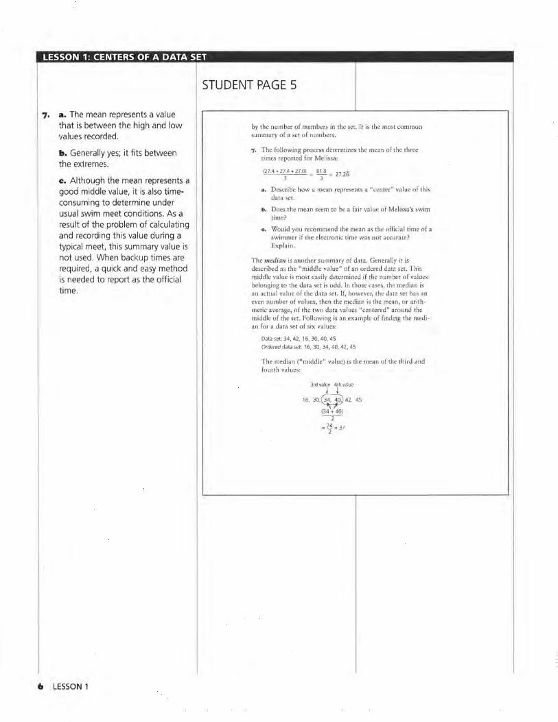
7. The following process determines the mean of the three times reported for Melissa:
(27.4 + 27.4 + 27.0) = ~ = 27 26 3 3 .
a. Describe how a mean represents a "center" value of this data set.
b. Does the mean seem to be a fair value of Melissa's swim time?
c. Would you recommend the mean as the official time of a swimmer if the electronic time was not accura te? Explain .
The median is another summary of data. Generally it is described as the "middle value" of an ordered data set. This middle value is most easily determined if the number of values belonging to the data set is odd. In those cases, the median is an actual value of the data set. If, however, the data set has an even number of values, then the median is the mean, or arithmetic average, of the two data values "centered" around the middle of the set. Following is an example of finding the median for a data set of six values:
Data set: 34, 42, 16, 30, 40, 45
Ordered data set: 16, 30, 34, 40, 42, 45
The median ("middle" value) is the mean of the third and fourth values:
3rd value 4th value
i i 16. 3o.C3c~o)42. 45
(34 + 40) - 2-
= zr = j/
LESSON 1: CENTERS OF A DATA SET
STUDENT PAGE 6
8. a. At least in this example, it is between the highest and lowest values recorded for Kristin.
b. Yes.
c. Shauna, like Kristin, has a good middle time with the criteria of the median. Melissa, however, does not have her times summarized by a "center" value using the median. This again highlights the usual feature of the collected times for Melissa.
9. a. Kristin's mean is 27.2 seconds, which is also the median.
b. This happens as 27 .2 seconds is in the middle of the other two times. Also, the other values have the same number of seconds above and below this middle value. Essentially 27 .2 is the average of the three times.
IO. Melissa; Melissa is the only swimmer who had two of her recorded times the same.
II. If a mode exists for a data set of three values, it is either the largest value or the smallest value of the set. (It cannot represent a middle value.)
IZ. If a mode exists for a data set of three, it is the same as the median.
I~. No. A data set of four or more will have a mode if two or more data values are equal. If two data values are equal out of four, then the mode could be the largest, the middle value, or the lowest value of the set. Although usual, the mode can also be described by more than one value. For example, the set {25, 25, 26, 26} is considered to have two modes, 25 and 26. This feature can be even more noticeable in data sets represented with more than 4 values. For this
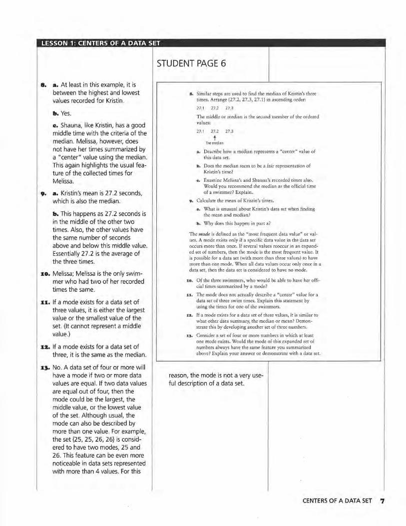
8. Similar steps are used to find the median of Kristin's three times. Arrange (27.2, 27.3, 27.1) in ascending order:
27.1 27.2 27.3
The middle or median is the second member of the ordered values:
27.1 27.2 27.3
t The median
a. Describe how a median represents a "center" value of this data set.
b. Does the median seem to be a fair representation of Kristin's time?
c. Examine Melissa's and Shauna's recorded times also. Would you recommend the median as the official time of a swimmer? Explain.
9, Calculate the mean of Kristin's times.
a. What is unusual about Kristin's data set when finding the mean and median?
b. Why does this happen in part a?
The mode is defined as the "most frequent data value" or values. A mode exists only if a specific data value in the data set occurs more than once. If several values reoccur in an expanded set of numbers, then the mode is the most frequent value. It is possible for a data set (with more than three values) to have more than one mode. When all data values occur only once in a data set, then the data set is considered to have no mode.
10. Of the three swimmers, who would be able to have her official times summarized by a mode?
11. The mode does not actually describe a "center" value for a data set of three swim times. Explain this statement by using the times for one of the swimmers.
1z. If a mode exists for a data set of three values, it is similar to what other data summary, the median or mean? Demonstrate this by developing another set of three numbers.
13. Consider a set of four or more numbers in which at least one mode exists. Would the mode of this expanded set of numbers always have the same feature you summarized above? Explain your answer or demonstrate with a data set.
reason, the· mode is not a very useful description of a data set.
CENTERS OF A DATA SET 7
14. a. Generally the median is a good middle value, although an exception was noted in Problem 12. The selection of the median is generally summarized for a set of three values as "throw out the high and the low"; this leaves a middle value for the official time. In a practical sense, the median is the easier summary to determine from a group of three timers. Frequently swim heats are run back to back, therefore, a quick and relatively accurate time is needed by the swim officials.
b. If there are three timers, then the median is very easy to determine (this again highlights the need for a quick and easy method to determine the swimmer's time). Expanding the number of timers will make this process more involved. If only two timers are used, then the official time is also the mean of the times recorded .
8 LESSON 1
STUDENT PAGE 7
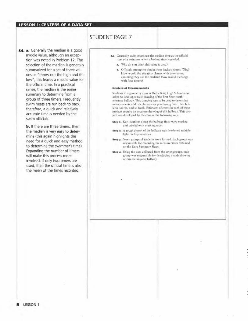
14. Generally swim meets use the median time as the official time of a swimmer when a backup time is needed.
a. Why do you think this value is used?
b. Officials attempt to obtain three backup timers. Why? How would the situation change with two timers, assuming they use the median? How would it change with four timers?
Centers of Measurements
Students in a geometry class at Rufus King High School were asked to develop a scale drawing of the first floor north entrance hallway. This.drawing was to be used to determine measurements and calculations for purchasing floor tiles, bulletin boards, and so forth. Estimates of costs for each of these projects require an accurate drawing of this hallway. This project was developed by the class in the following way:
Step 1. Key locations along the hallway floor were marked and labeled with maskmg rape.
Step 2. A rough sketch of the hallway was developed to highlight the key locations.
Step~. Seven groups of students were formed. Each group was responsible for recording the measurements obtained on· the Data Summary Sheet.
Step 4, Using the data collected from the seven groups, each group was responsible for developing a scale drawing of this rectangular hallway.
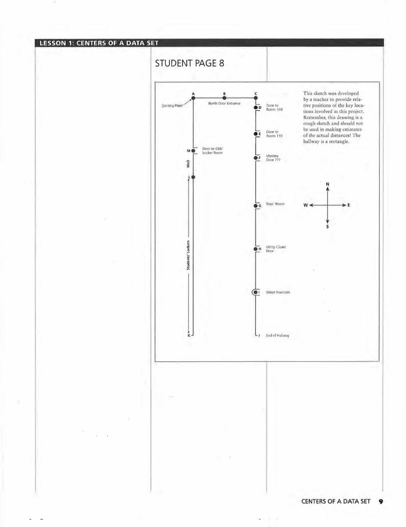
LESSON 1: CENTERS OF A DATA SET
STUDENT PAGE 8
A 0 c This sketch was developed -Starting Pomt/.
- l.. by a teacher to provide rela-North Door Entrance
Door to tive positions of the key loca-eo
[ Room 109 tions involved in thi.s project.
Remember, this drawing is a rough sketch and should not
Door to be used in making estimates .E Room 110 of the actual distances! The
[ hallway is a rectangle. - Door to Girls' Me Locker Room - .F Mystery
- Door 1??
~
LO
N
- Boys' Room w+• .G
l s
~ ~
Utility Closet ~ .H - Door
l!l c ~ ,, ~
-~ Water Fountain
K End of Hallway
CENTERS OF A DATA SET 9
LESSON 1: CENTERS OF A DATA SET
STUDENT PAGE 9
15. a. Errors in measuring, differences in measuring tools, slight differences in starting and ending points of the distances measured, or other answers could be summarized by students. Students might be asked this question again after they attempt the Further Practice section as the actual process of measuring distances helps them understand the potential for errors.
b. Completing the values for this table is rather tedious. This problem takes quite a bit of time. As a result, this problem is ideal for group work.
Data Summary lor the Measurement Experiment Rufus King Hllh School North Entrance Hallway (meters)
Group AB BC CD DE EF FG GH Group 1 1 78 1 77 0.65 8 34 1 87 5.02 2_10
Group 2 1 78 1 75 0.58 9 35 1 85 498 1 75
Group 3 1.77 1.75 0.59 920 188 4.95 2 25
Group 4 1 78 1 76 066 910 1 90 5,03 1 95
Group 5 1 75 1 80 0 67 9 OS 1 89 4.95 2 23
Group 6 1.68 1.76 0.63 9.10 1.88 4.80 2. 15
Group 7 1.78 1.76 0.66 8 91 1 87 5, 10 2 17
Mean
Median
Mode
Group HI IJ JK KL LM MA
Group 1 3 34 3 08 3 55 8.88 5 30 11 32
Group 2 3 96 3.50 3.65 9.52 5.00 10.91
Group 3 3 55 3.64 3.56 9. 14 5 62 12 12
Group 4 3. 12 2.68 3 72 8 78 5 45 11 52
Group S 3 OS 2 85 343 8 68 515 13 58
Group 6 3 22 2 98 3.31 8 94 5 23 9 12
Group 7 3.40 3 05 3.33 11.25 5.35 11 56
Mean
Median
Mode
:15. Using the class measurements, answer the following questions before developing a scale drawing.
a. Review the data sets. Each group was expected to measure the same distances. Why are the recorded measurements different?
b. Complete the data sheet by determining the means, medians, and modes for each of the distances labeled. Copy and complete this part of the data sheet.
c. You will be developing a scale drawing of this rectangular hallway. What do you anticipate to be the main problem in constructing an accurate sketch of this hallway?
:1c.. Consider the following four criteria in selecting the "best" center of the measurements reported by the groups.
•the mean of the values for any of the specified distances
• the median of the values
Data Summary Sheet for the Measurement Experiment c. The primary concern is to deter-Rufus King High School North Entrance Hallway (meters) mine what measure or what sum-
Group AB BC CD DE EF FG GH mary of the measures should be used to develop the scale drawing.
Mean 1.76 1.76 0.63 9.01 1.88 4.98 2.09
Median 1.78 1.76 0.65 9.10 1.88 4.98 2.15
Mode 1.78 1.76 0.66 9.10 1.87, 1.88 4.95 none
Group HI IJ JK KL LM MA
Mean 3.38 3.11 3.51 9.31 5.30 11.45
Median 3.34 3.05 3.55 8.94 5.30 11 .52
Mode none none none none none none
10 LESSON 1
LESSON 1: CENTERS OF A DATA SET
STUDENT PAGE 10
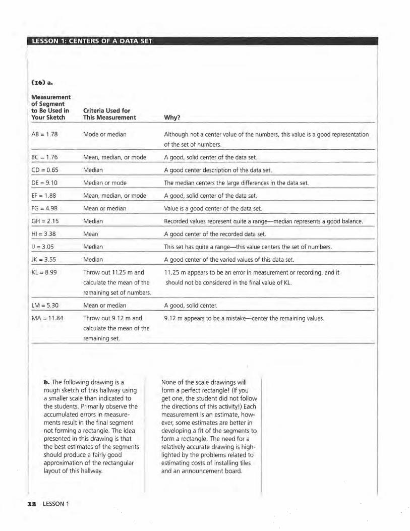
16. Students should be encouraged to select their own values and justify their selection. The following values are used to develop a scale drawing of the hallway and provides an example of the process described in this lesson. The measures used for each segment will vary from student to student (or from group to group).
•the mode of the values (if one exists)
•an "average" (mean or median) of a subset of the values
(The last criterion allows some measurements to be thrown out as obvious errors. The measurements remaining would then be averaged or "centered.")
11. Determine the measurements you will use to develOp the scaled sketch of the rectangular hallway. Explain what criterion you used to select this best estimate and why. Complete the following table which is also on Activity Sheet 1.
Measurement of Criteria used segment to be for this used in your sketch measurement Why?
AB=
BC=
CD=
DE=
Ef =
FG=
GH=
HI=
IJ =
JK =
KL=
LM=
MA=
b. Develop a scale drawing of this hallway based on the measurements selected in your table. Begin developing this scale drawing by placing the starting point A in the upper-left corner of a blank sheet of paper. (You might consider developing this sketch on legal size paper as this hallway is quite long.) Measure and mark each of the labels provided in the teacher's sketch of this hallway. Use a scale of 1 cm = 1 meter or a comparable scale.
CENTERS OF A DATA SET 11
LESSON 1: CENTERS OF A DATA SET
Measurement of Segment to Be Used in Your Sketch
AB= 1.78
BC= 1.76
CD= 0.65
DE= 9.10
EF = 1.88
FG = 4.98
GH = 2.15
HI= 3.38
IJ = 3.05
JK = 3.55
KL= 8.99
LM = 5.30
MA= 11.84
Criteria Used for This Measurement
Mode or median
Mean, median, or mode
Median
Median or mode
Mean, median, or mode
Mean or median
Median
Mean
Median
Median
Throw out 11.25 m and
calculate the mean of the
remaining set of numbers.
Mean or median
Throw out 9.12 m and
calculate the mean of the
remaining set.
b. The following drawing is a rough sketch of this hallway using a smaller scale than indicated to the students. Primarily observe the accumulated errors in measurements result in the final segment not forming a rectangle. The idea presented in this drawing is that the best estimates of the segments should produce a fairly good approximation of the rectangular layout of this hallway.
I2 LESSON 1
Why?
Although not a center value of the numbers, this value is a good representation
of the set of numbers.
A good, solid center of the data set.
A good center description of the data set.
The median centers the large differences in the data set.
A good, solid center of the data set.
Value is a good center of the data set.
Recorded values represent quite a range-median represents a good balance.
A good center of the recorded data set.
This set has quite a range-this value centers the set of numbers.
A good center of the varied values of this data set.
11.25 m appears to be an error in measurement or recording, and it
should not be considered in the final value of KL.
A good, solid center.
9.12 m appears to be a mistake-center the remaining values.
None of the scale drawings will form a perfect rectangle! (If you get one, the student did not follow the directions of this activity!) Each measurement is an estimate, however, some estimates are better in developing .a fit of the segments to form a rectangle . The need for a relatively accurate drawing is highlighted by the problems related to estimating costs of installing tiles and an announcement board.

LESSON 1: CENTERS OF A DATA SET
Note how segments do not meet to form the rectangle .
A/ c
K .__ __ __,
x7. The individual segments will not fit together to form the rectangle. Either the final segment is under or over the value needed to make a fit of the segments as a rectangle .
xs. Total measures of the widths and lengths should be equal. Comparing widths indicates AC = 3.54 m and JK = 3.55 m. Comparing lengths indicates CJ= 25.19 m and KA= 26.13 m. Differences are expected given the way the measurements were made.
x9. The larger segments show more variation and are probably more subject to error. For example, segments MA. KL, and DE are more difficult to estimate given the variations noted in the measurements.
STUDENT PAGE 11
I7, Your drawing represented the best measures of the distances given your criteria. As you compare your sketch to other members of the class, how does each sketch indicate the measures are not "perfect"?
I8. How could the fact that the hallway is rectangular help in developing an accurate sketch?
I9. Of the measurements recorded on the data sheet, what specific distances do you think are the most likely to be inaccurate. Explain why you think this.
zo. A group of students studying the collected data commented that the Rufus King students obviously used meter sticks (rulers) instead of a measuring tape. Would you agree? Explain your answer.
SUMMARY
Collected data frequently needs to be summarized by a center. Mean, median, or mode are summaries of a data set representing frs "center" or summary.
Practice and Applications
ZI. From your sketch, determine the following distances:
a. the distance (to the nearest meter) from the door of room 109 to the girls' locker room door.
b. the distance from the water fountain to point A.
c. the distance from the boys' room door to the girls' locker room door.
zz. If floor tiling will be installed at a cost of $16.75 per square meter, what is your estimate of the total cost of installing floor tiles for the entire hallway?
z:J, An announcement board for the athletic department will be installed from point A to a point 1 meter north of the girls' locker room door (or 1 meter north of point M). If your scale drawing is used to estimate the length of the board, what problem do you encounter with this last segment of the drawing?
z4. If the announcement board discussed in problem 23 costs $10. 70 per linear meter, what is the projected total cost of this project? (The announcement board has a standard height, therefore, your estimates do not need to involve that dimension of the board.)
zo. This conjecture is based on the more noticeable differences in the larger measurements, something more likely when placing meter sticks back to back. Students might be interested in testing out this idea. Mark a distance of at least 10 meters and have three or four groups measure the distance. Collect estimates from each group based on the use of a meter stick and a tape measure.
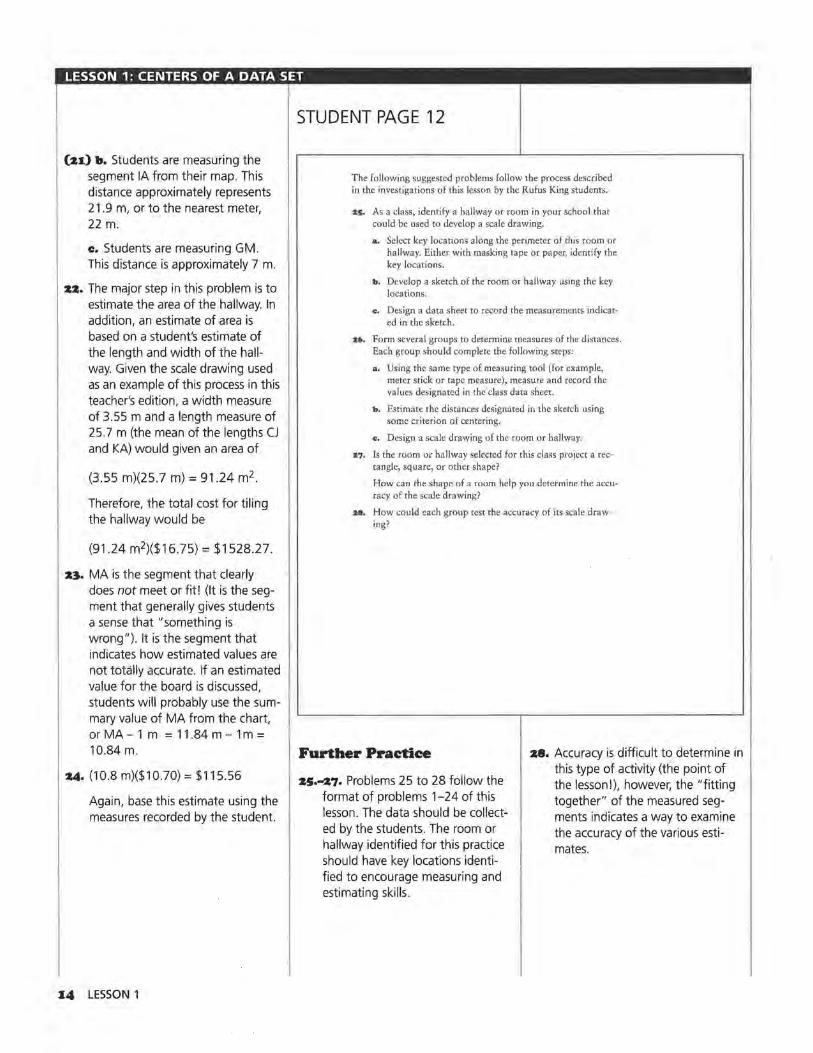
Practice and Applications
zx. The distances provided by the students should be based on their scaled drawing. The following distances are approximations based on the measurements used in problem 15:
a. Students are measuring the segment OM from their scaled drawing. This distance is 10.4 cm, therefore, representing 10.4 m. To the nearest meter, this is 10 m.
CENTERS OF A DATA SET J.3
LESSON 1: CENTERS OF A DATA SET
(21) b. Students are measuring the segment IA from their map. This distance approximately represents 21.9 m, or to the nearest meter, 22 m.
c. Students are measuring GM. This distance is approximately 7 m.
22. The major step in this problem is to estimate the area of the hallway. In addition, an estimate of area is based on a student's estimate of the length and width of the hallway. Given the scale drawing used as an example of this process in this teacher's edition, a width measure of 3.55 m and a length measure of 25.7 m (the mean of the lengths CJ and KA) would given an area of
(3.55 m)(25.7 m) = 91.24 m2 .
Therefore, the total cost for tiling the hallway would be
(91.24 m2)($16.75) = $1528.27.
2~. MA is the segment that clearly does not meet or fit! (It is the segment that generally gives students a sense that "something is wrong"). It is the segment that indicates how estimated values are not totally accurate. If an estimated value for the board is discussed, students will probably use the summary value of MA from the chart, or MA - 1 m = 11 .84 m - 1 m = 10.84 m.
24. (10.8 m)($10.70) = $115.56
Again, base this estimate using the measures recorded by the student.
14 LESSON 1
STUDENT PAGE 12
The following suggested problems follow the process described in the investigations of this lesson by the jlufus King students.
zs. As a class, identify a hallway or room in your school that could be used to develop a scale drawing.
a. Select key locations along the perimeter of this room or hallway. Either with masking tape or paper, identify the key locations.
b. Develop a sketch of the room or hallway using the key locations.
c. Design a data sheet to record the measurements indicated in the sketch.
zc.. Form several groups to determine measures of the distances. Each group should complete the following steps:
a. Using the same type of measuring tool (for example, meter stick or tape measure), measure and record the values designated in the class data sheet.
b. Estimate the distances designated in the sketch using some criterion of centering.
c. Design a scale drawing of the room or hallway.
z7. Is the room or hallway selected for this class project a rectangle, square, or other shape?
How can the shape of a room help you determine the accuracy of the scale drawing?
zs. How could each group test the accuracy of its scale drawing?
Further Practice
2s.-z7. Problems 25 to 28 follow the format of problems 1-24 of this lesson. The data should be collected by the students. The room or hallway identified for this practice should have key locations identified to encourage measuring and estimating skills.
28. Accuracy is difficult to determine in this type of activity (the point of the lesson!), however, the "fitting together" of the measured segments indicates a way to examine the accuracy of the various estimates.
LESSON 2
Descriptions Through Centers Materials: tape measure, Activity Sheets 2 and 3, Unit I Quiz
Technology: graphing calculator
Pacing: 1 to 2 class sessions
Overview
Lesson 2 continues the description of center as a summary of data and develops additional activities to get students involved in collecting data. This lesson works, however, on another dimension-namely the possible connection of two data sets. This connection could be expanded through a study of linear relations and a best-fitting line. These extensions are given a more thorough treatment in other modules of this series. This lesson primarily asks students to summarize the relationship suggested by collected data. This may seem a general treatment of scatter plots for students who have previously worked with them. The precision some students might expect is not developed in this lesson because the primary goal is to emphasize the importance of data summaries (i.e., centers) and not linear relations.
Teaching Notes
This lesson extends the type of applications requiring a summary of data described as a center. This lesson complements the first lesson by highlighting problems involved in communicating the results of a collection of data. This lesson was particularly important in demonstrating how different centers could be used to summarize data and produce varying conclusions about the data.
Preparation is recommended in determining a location for students to collect the data for walking the 50-m distance. Also, a tape measure used for recording students' heights should be set up before the lesson is attempted.
Technology
Several questions require tedious calculations. As indicated in Lesson 1, this process requires the use of a scientific or graphing calculator. At this point, the problems do not require the special features of a graphing calculator. The lesson concludes with a look at a scatter plot of data. The lesson directs the students producing this scatter plot to use the grids provided by the activity sheet. However, implementing this scatter plot using a graphing calculator could be developed. The format of producing the graphs is a teacher decision. (The use of scatter plots for the investigation of linear relations is presented thoroughly in other modules of this series. This lesson reviews these topics but does not give a formal presentation of linear regression topics.)
Follow·Up
This lesson suggests several follow-up activities within the lesson. These activities can be modified or developed depending on the students abilities in completing the stated objectives. The quiz for Unit I is designed to review the collection activities developed in the lessons and the process of summarizing the data using a center. The assessment, or quiz, in this particular unit is designed to follow a format similar to the problems presented in the lessons.
DESCRIPTIONS THROUGH CENTERS IS
LESSON 2: DESCRIPTIONS THROUGH CENTERS
Solution Key
Discussion and Practice
1. a. The coordination described in the problem maximizes the jumper's momentum and ability to put forces together for obtaining distance.
b. Jumper's height, physical development or conditioning, leg length, or similar answers of this type are appropriate.
I6 LESSON 2
STUDENT PAGE 13
LESSON 2
Descriptions Through Centers
Have you ever watched athletes competing in track and field events?
What kind of special preparation would be necessary for competing in an event such as the broad jump?
T rack and field events require athletes to coordinate running and jumping skills. Athletes participating in the high
or low hurdles spend considerable time counting the number of steps needed to reach a position to begin the jump over a hurdle . Incorrectly counting' the number of steps can throw off the coordination and the resulting time for the athlete to complete the event. Similarly, the broad jump event in track and field also requires athletes to coordinate running and jumping.
INVESTIGATE
Track and Field Events
Olympian Carl Lewis carefully prepared for several summer Olympics (and subsequent world records in the broad jump) by running a specific distance and counting his steps or strides before making the actual jump. How might Carl determine the number of steps to the jumping-off line?
Discussion and Practice
1. Consider the broad jump event in a track and field meet.
a, Why is it important to coordinate running and jumping with this event?
II. What are some factors that might affect the number of steps or strides of a particular broad jumper?
Calculate the mean, median, and mode of a
data set
Interpret a center as an estimation of a data set
Interpret a center as a description of an
individual's physical characteristics.
LESSON 2: DESCRIPTIONS THROUGH CENTERS
z. Answers will vary; possible answers include: measure length of one step and divide this length per step into 50 m; or, walk 50 m and count your number of steps.
~. a. 50 m I 0.85 m per step = 58.8 steps or approximately 59 steps.
b. A description based on one step suggests a high potential for error. One of the main points of this lesson is to sense how a summary of this type is better determined by an finding an average.
c:. One method would be to walk a distance of 50 m and count the number of steps .
4. Answers will vary on this problem. It may be necessary to set a different "standard" than 85 cm based on the results from volunteers.
a. This material was field tested with 9th and 10th graders. Using 85 cm as the standard, the taller students were clearly in one group. It might also be summarized by students that groups were determined by gender. However, at this age, males were generally taller in the field-test groups. Students 6 ft or taller were frequently in the group with steps measuring 85 cm or more.
b. Again, students shorter than 6 ft were in the group measuring 85 cm or less. Change the 85 cm to a value that more appropriately demonstrates the relationship to height given the students physical characteristics in your class.
STUDENT PAGE 14
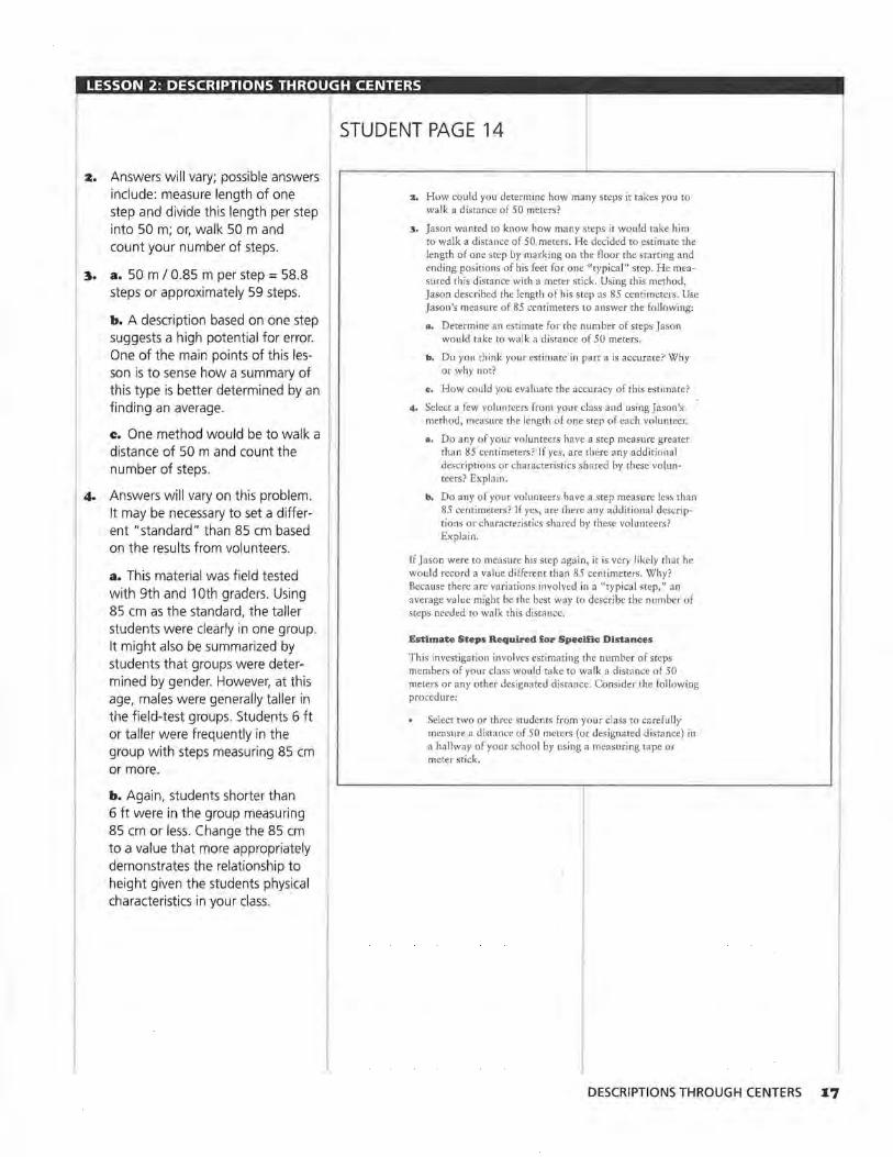
:&. How could you determine how many steps it takes you to walk a distance of 50 meters?
3, Jason wanted to know how many steps it would take him to walk a distance of 50 meters. He decided to estimate the length of one step by marking on the floor the starting and ending positions of his feet for one "typical" step. He measured this distance with a meter stick. Using this method, Jason described the length of his step as 85 centimeters. Use Jason's measure of 85 centimeters to answer the following:
a. Determine an estimate for the number of steps Jason would take to walk a distance of 50 meters.
b. Do you think your estimate in part a is accurate? Why or why not?
c. How could you evaluate the accuracy of this estimate?
4, Select a few volunteers from your class and using Jason's method, measure the Jength of one step of each volunteer.
a. Do any of your volunteers have a step measure greater than 85 centimeters? If yes, are there any additional descriptions or characteristics shared by these volunteers? Explain.
b. Do any of your volunteers have a step measure less than 85 centimeters? If yes, are there any additional descriptions or characteristics shared by these volunteers? Explain.
If Jason were to measure bis step again, it is very likely that he would record a value different than 85 centimeters. Why? Because there are variations involved in a "typical step," an average value might be the best way to describe the number of steps needed to walk this distance.
Estimate Steps Required £or Specific Distances
This investigation involves estimating the number of steps members of your class would take to walk a distance of 50 meters or any other designated distance. Consider the following procedure:
Select two or three students from your class to carefully measure a distance of 50 meters (or designated distance) in a hallway of your school by using a measuring tape or meter stick.
DESCRIPTIONS THROUGH CENTERS I7
LESSON 2: DESCRIPTIONS THROUGH CENTERS
5. Explanations will obviously vary, but it is unlikely the results will be the same for all five trials. The variable numbers can be explained by the problem with how to count the last step, the way a person walks (i.e., rigid and precision walking to a casual and uneven walking), mistakes in counting, uneven steps, etc.
6. Answers to the following problems depend on the collected data . By designing this problem around five trials, the likelihood for a mode is increased . Observing a mode, or a meaningful mode, however, is not important. Collecting this data and developing summaries is the main point of this part of the lesson.
a. Use the collected data.
b. Use the collected data .
e. Use the collected data .
d. Use the collected data .
7. Answers will again vary dependent on the collected data.
a. Use the collected data .
b. Use the collected data.
e. Use the collected data.
18 LESSON 2
STUDENT PAGE 15
Mark a convenient starting and ending point on the floor of the hallway with masking tape.
When given permission by your teacher, as many members of your class as possible should walk (do NOT run, jump, or skip for now) the measured distance of 50 meters (or designated distance) and count the number of steps it took each person to reach the end position.
If you walked this distance, record your count as the result for Trial 1. Repeat this procedure by walking this same distance for four additional trials. For each trial, record the approximate number of steps counted. (Do not worry about any fractional step needed to reach the end position. Use your best judgment to estimate whether or not to count the last step. Record all trials as whole numbers.)
Your Name Tria1
1 Trial
2 Trial
3 Trial
4 Trial
5
5, Did you expect to record the same number of steps for each of your trials? Why or why not?
6. Conduct a poll of the students in your class who walked the distance described.
a. How many students recorded the same number of steps for all five trials?
b. How many students recorded a different number for each of the five trials?
a. How many students had four trials the same?
d. How many students had two trials the same?
7, Determine the following summaries of the five trials you recorded.
a. the mean of the five trials
b. the median of the trials
c. the mode of the five trials (provided a mode value exists)
LESSON 2: DESCRIPTIONS THROUGH CENTERS
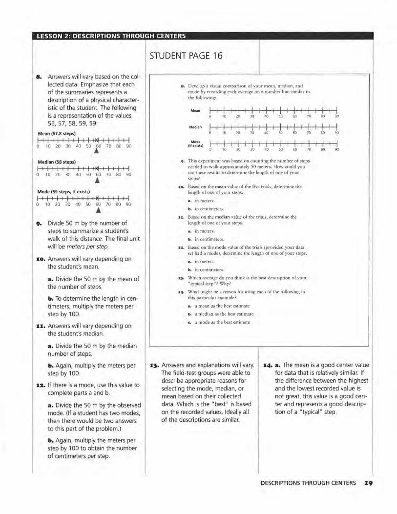
8. Answers will vary based on the col-lected data. Emphasize that each of the summaries represents a description of a physical character-istic of the student. The following is a representation of the values 56, 57, 58, 59, 59:
Mean (57 .8 steps)
I I I I I I I I I I I !><I I I I I I I 0 10 20 30 40 50 l.o 70 80 90
Median (58 steps)
I I I I I I I I I I I l ><I I I 1 I I I 0 10 20 30 40 50 60 70 80 90 • Mode (59 steps, if exists)
I I I I I I I I I I I I ~ I I I I I I 0 10 20 30 40 50 60 70 80 90 • 9. Divide 50 m by the number of
steps to summarize a student's walk of this distance. The final unit will be meters per step.
10. Answers will vary depending on the student's mean .
a. Divide the 50 m by the mean of the number of steps.
b. To determine the length in centimeters, multiply the meters per step by 100.
11. Answers will vary depending on the student's median .
a. Divide the 50 m by the median number of steps.
b. Again, multiply the meters per step by 100.
12. If there is a mode, use this value to complete parts a and b.
a. Divide the 50 m by the observed mode. (If a student has two modes, then there would be two answers to this part of the problem.)
b. Again, multiply the meters per step by 100 to obtain the number of centimeters per step.
STUDENT PAGE 16
8. Develop a visual comparison of your mean, median, and mode by recording each average on a number line similar to the following:
Mean I I I I I I 0 10 20 30 40 50 60 70
Median I I I I I I 10 20 30 40 50 60 70
Mode I I I I I (if exists) 10 20 30 40 50 60 70
9. This experiment was based on counting the numbe.r of steps needed to walk approximately 50 meters. How could you use these results to determine the length of one of your steps?
10. Based on the mean value of the five trials, determine the length of one of your steps.
a. in meters.
b. in centimeters .
11. Based on the median value of the trials, determine the length of one of your steps.
a. in meters.
b. in centimeters.
12. Based on the mode value of the trials (provided your data set had a mode), determine the length of one of your steps.
a. in meters.
b. in centimeters.
13. Which average do you think is the best description of your "typical step"? Why?
14. What might be a reason for using each of the following in this particular example?
a. a mean as the best estimate
b. a median as the best estimate
c. a mode as the best estimate
I 80 90
I I 80 90
I 80 90
1~. Answers and explanations will vary. The field-test groups were able to describe appropriate reasons for selecting the mode, median, or mean based on their collected data. Which is the "best" is based on the recorded values. Ideally all of the descriptions are similar.
14. a. The mean is a good center value for data that is relatively similar. If the difference between the highest and the lowest recorded value is not great, this value is a good center and represents a good description of a "typical" step .
DESCRIPTIONS THROUGH CENTERS J.9
LESSON 2: DESCRIPTIONS THROUGH CENTERS
b4) b. The median (especially for a data set of 5) is a good center value. It is particularly useful when the difference between the highest or lowest is great. The median cancels out the extremes whereas the mean builds these values into the center.
c. Modes are easy to spot as good descriptions when it is between the highest and lowest values. The mode is not as good a description when it is a representation of either the highest or lowest value. Also, it is possible a mode does not exist for a particular student.
is. Answers will depend on the collected data from the class. It is not always clear why a student is selecting the specific value of a median, mode, or mean, but variation with in the class provides a good comparison of students' physical characteristics.
16. Students should mark their recorded values from approximately 13 other students. This visual should suggest the connections discussed in the remaining problems in this lesson.
17. This problem again seems to suggest connecting steps with height, or possibly leg length or athletic development.
a. Results depend on the collected data.
b. In the field-test groups, this generally identified the taller students.
ZO LESSON 2
STUDENT PAGE 17
15. Select mean, median, or mode. Collect at least 13 averages of this type from studerits in your class. In other words, collect 13 means or 13 medians or 13 modes from the other students involved in this project. Do not mix the Lype of averages collected from the other members of your class! Copy and complete the following table:
Average selected in your sample: --------(Mean, median, or mode}
Name Number of Steps
u .. Visually represent the results of the 13 summaries you collected by plotting the value for each student on the num-ber lines provided on Activity Sheet 2. Include your summa-ry in this collection.
You I I I I I I 10 io JO 40 50 60
Student 1 I I I I I I 0 10 20 30 40 50 60
Student 2 I I I I I I I 0 10 20 30 40 50 60
• • • Student 13 I I I I I I I
0 10 20 30 40 50 60
17. Examine the data collected from your class.
a. Identify the two students in your data set who recorded the fewest number of steps.
b. Identify the. two students in your data set who recorded the greatest number of steps.
I I I 70 80 90
I I I 70 80 90
I I I 70 80 90
I I Jo I 70 80
LESSON 2: DESCRIPTIONS THROUGH CENTERS
b7) c. Height, leg length, forearm length, etc.
18. a. Months of birthdays, shoe size, and number of brothers and sisters showed no connections. Students generally did not suspect these characteristics but it provided a way to discuss connections. Number of sit-ups is a bit more complicated as it might be indirectly connected to other descriptions such as height, etc.
b. Height or forearm lengths were excellent selections to complete the rest of the problems. (However, some variation in developing these problems provides excellent discussions.) As a class, define the way a forearm, leg length, etc. is measured. For the field-test group, leg length was measured from the waist to the floor as a student stood straight.
c. Students complete the table for themselves and the 13 students selected from Problem 16.
STUDENT PAGE 18
c. As you consider the students identified in parts a and b, are there any descriptions or characteristics that distinguish the students who recorded the fewest number of steps from the students who recorded the greatest number of steps?
:i:s. Consider the following additional descriptions or character-istics of the students in your class.
Month of their birthdays (January= 1, February= 2, etc.)
Height (in inches or centimeters)
Length of their forearms (in inches or centimeters)
Shoe size
Number of brothers and sisters
Circumference of wrists (in inches or centimeters)
Number of sit-ups completed in 30 seconds
a. Which descriptions or characteristics in the list above do you think would not distinguish the students who recorded the fewest number of steps from the students who recorded the greatest number of steps?
b. Select one of the additional descriptions or characteristics you think might distinguish the two groups of students and explain why you selected this item.
c. Collect from the 13 students in your sample the value corresponding to the characteristic you selected in part b. Organize this additional piece of data in a chart similar to the one below.
Student Additional Description (x-value)
Number of Steps (y-value)
DESCRIPTIONS THROUGH CENTERS ZI
LESSON 2: DESCRIPTIONS THROUGH CENTERS
1:9. Plotting the resulting points is not to be interpreted as a thorough treatment of correlation or other topics of linear regression. Simply use the points as a way to highlight a pattern or possible relationship of the two values. In the field-test groups, the general pattern was summarized by the observation that "as the heights of students increased, the number of steps needed to walk 50 m decreased."
zo. Although the answers depend on the descriptions selected, generally the graphs involving heights or forearms were connected as summarized in problem 19. Several of the other items did not indicate a pattern from the scatter plot.
The general pattern of the points suggests the connection. In the case of height or forearm length, a general line could be used to describe the connection. Although this could be developed into discussions of correlation, a general linear relation is a sufficient response to a suggestion of the relationship of the points. Details of correlation are left for other modules within this series.
zi:. Running the distance will change the results noticeably! In addition, if a student ran this distance for several trials, differences in the outcomes will be more obvious than the results for walking. This problem is not based on actually collecting the data by running the distance, but basically on a student's guess or conjecture. As a result, answers will vary. If possible, a small sample of students selected to run this distance might enrich this discussion. Develop this extension with a data sheet examining
ZZ LESSON 2
STUDENT PAGE 19
19. Using the x- and y-values as indicated in the chart, plot the points representing your sample of students on a coordinate grid similar to the one below. You may use Activity Sheet 3.
:zo. Do the points you plotted in problem 19 indicate a relationship between the Additional Description and the number of steps? If so, describe the relationship.
:11. If you were allowed to run the 50-meter distance, how would the number of strides counted in this distance change?
SUMMARY
A value used to describe the length of a person's step or the number of steps needed for a person to walk a specific distance may best be described as a center of a data set. A mean, median, or mode can be used to identify the center.
When two variables are investigated, a coordinate grid may be used to visualize their relationship.
the number of steps involved in walking the distance and the number of steps involved in running the distance.
LESSON 2: DESCRIPTIONS THROUGH CENTERS
Practice and Applications
22. (Note: The distances involved are in yards and not meters. This changes the recorded values from those collected by the class.)
a. 42.833
b. For values 41, 42, 42, 43, 44, and 45; the median is 42.5.
c. 42
23. Note: The chart involved in this problem organizes the data with the x-value as the number of steps. This is the reverse of what was set up in the Investigate section where they-values represented the recorded step values. This is intentional as the goal is to think about a connection that is not involved in a cause-and-effect discussion. This is best achieved by making the roles of the x- or y-values interchangeable.
James Rockweger's height is highly suspect to error, especially given his recorded number of steps to walk the 30 yards.
24. The following graph excludes the recorded value for James Rockweger:
~
-<=
80
75 x
.£' 70 .,
QI
:r
65
60 36 38 40
Steps
:k x
f 42 44 46
Note: This graph was generated by a spreadsheet program. A similar scatter plot could also be developed by a graphing calculator or by hand using a coordinate grid. Teachers can define their own
STUDENT PAGE 20
Practice and Applications
zz. Corey Reed collected the following data or number of steps taken as he walked a distance of 30 yards (note: this distance is measured in yards):
42, 41, 44, 43, 42, 45
a. Determine the mean of Corey's data set:
b. Determine the median of Corey's data set:
c. Determine the mode of Corey's data set:
z~. Corey also collected the height and mean number of steps for several other students in his class. He recorded his collected data in the following chart:
Number of Height in Name steps(x) inches (y)
Sam Bland 37 74
Robert Rotella 38 76
Claud Salyards 42 68
James Rockweger 41 41
Devon Brooks 40 72
Anthony Balistreri 45 67
Rachel Jones 44 64
Jeffrey Durr 43 70
Laura Frye 42 69
Study the data set recorded by Corey. He might have erred in measuring! Corey most likely erred in measuring the height of which person? Explain why you think this measurement (or measurements) was incorrect.
Z4· Develop a scatter plot of the values indicated in the chart of problem 23 on a coordinate grid provided on Activity Sheet 3. DO NOT include any values from the data set you think represent an error in Corey's measurement.
zs. Does height seem to be related to the mean number of steps recorded to walk 30 yards? Why or why not?
zf>. Estimate James Rockweger's height. How did you determine this estimate?
z7. Estimate Corey's height. How did you determine this estimate?
requirements regarding the scales used for the x- and y-axes.
2s. There does seem to be a pattern demonstrated with this data. In this case, the number of steps seems to be connected to the height, or "as the number of steps needed to walk 30 yards increased, the height of the students decreased."
26. Answers will vary, but an estimate of a line fitting the scatter plot
would suggest James Rockweger's height to be 70 to 71 inches.
27. If you used 42 as his average (the mode value from his collected data set), then his height, suggested by the same line used in problem 26, is 68 to 70 inches.
DESCRIPTIONS THROUGH CENTERS Z3

UNIT II
Centers of Balance

LESSON 3
The Mean as a Center of Balance Materials: rulers and raisins
Technology: graphing calculator Pacing: 2 class sessions
Overview
This is the first of several lessons in which the mean is singled out as an especially important summary of a center. The first application of mean is directed at a location representing a center of balance. Balance is also expanded in other lessons of this module. The difficulty with this particular lesson is related to implementing the hands-on activities described and illustrated. Students are directed to place raisins along a centimeter ruler. Using the broad side of a pencil, students are asked to find a position along the ruler that balances the arrangement. The questions and problems related to the observations of the raisins and the ruler are not designed as precise experiments. Although raisins are described as "objects of approximately equal weight," the slight differences in the weights of raisins and in the rulers will contribute to different results from student to student. Even though precision is not emphasized, the process of developing a hands-on "feel" for a center of balance was highlighted as important by the field-test teachers.
Teaching Notes
This lesson is significant in setting up the work for lessons outlined later in this module. The role of a mean as a location along a number line providing balance is worked through several applications and examples throughout this module. Although students have worked with mean previously, this could be their first experience discovering the mean as outlined in this lesson. Closely related to this introduction of a balance point are the extensions of the mean to a weighted mean as presented in,Lesson 4. Although
possibly not obvious at this point in the module, this is an important lesson in setting the stage for the applications involved in population centers.
Organizing a hands-on component as outlined in the lesson is important and should be planned during the preparation of this lesson. (Logistics involved in providing the rulers and raisins to each student are important in estimating a time frame for this lesson.) This lesson can be introduced early in a geometry class since geometric references are minimal.
Follow· Up
Art, physics, and several other disciplines might also be incorporated in demonstrating to students a center of balance. Engineers involved in the design of aircraft, bowling pins, cars, bridges, and so on, are continually analyzing balance points. Information on the safety standards for cars, set up to rectify inappropriate centers of balance, are available and could be used to further the discussions presented in this lesson. These topics could be investigated by general searches on the Internet and/or consumer periodicals.
THE MEAN AS A CENTER OF BALANCE 27
LESSON 3 : THE MEAN AS A CENTER OF BALANCE
Z8 LESSON 3
STUDENT PAGE 23
LESSON 3
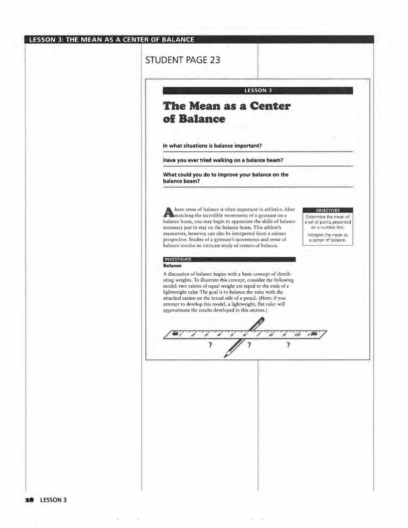
The Mean as a Center of Balance
In what situations is balance important?
Have you ever tried walking on a balance beam?
What could you do to improve your balance on the balance beam?
A keen sense of balance is often important in athletics. After watching the incredible movements of a gymnast on a
balance beam, you may begin to appreciate the skills of balance necessary just to stay on the balance beam. This athlete's maneuvers, however, can also be interpreted from a science perspective. Studies of a gymnast's movements and sense of balance involve an intricate study of centers of balance.
INVESTIGATE
Balance
A discussion of balance begins with a basic concept of distributing weights. To illustrate this concept, consider the following model: two raisins of equal weight are taped to the ends of a lightweight ruler. The goal is to balance the ruler with the attached raisins on the broad side of a pencil. (Note: if you attempt to develop this model, a lightweight, flat ruler will approximate the results developed in this section.)
?
Determine the mean of a set of points presented
on a number line.
Interpret the mean as a center of balance.
LESSON 3: THE MEAN AS A CENTER OF BALANCE
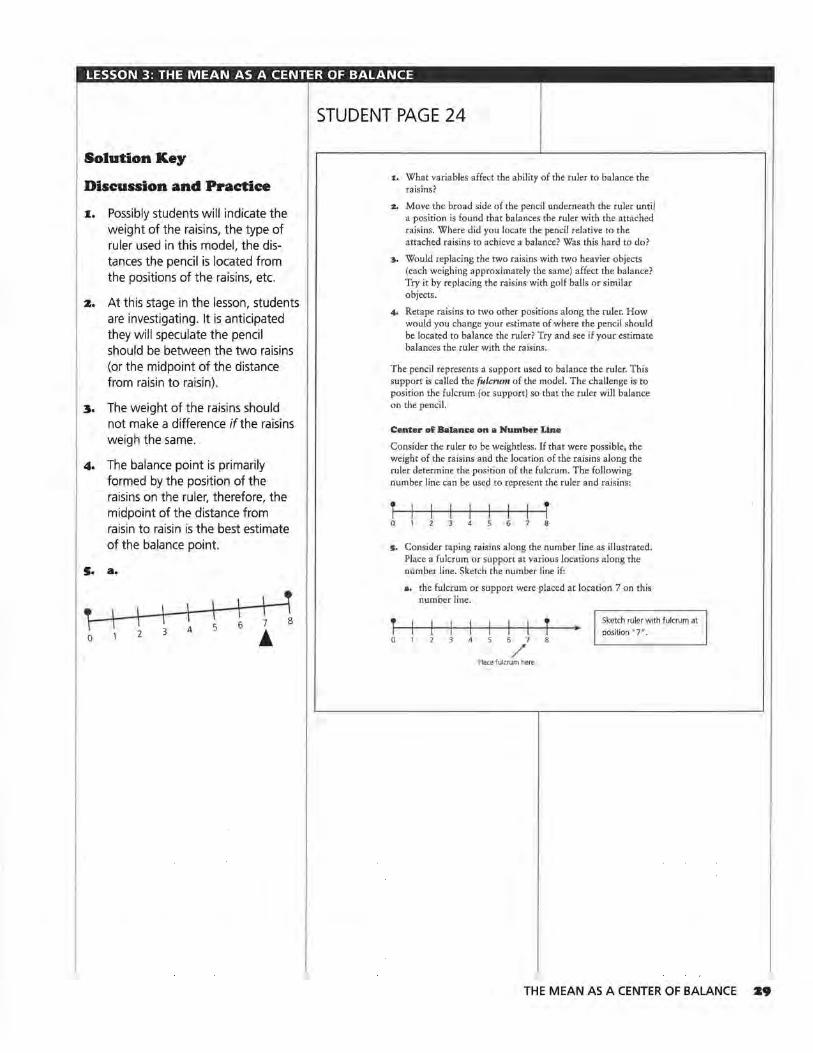
Solution Key
Discussion and Practice
1. Possibly students will indicate the weight of the raisins, the type of ruler used in this model, the distances the pencil is located from the positions of the raisins, etc.
z. At this stage in the lesson, students are investigating. It is anticipated they will speculate the pencil should be between the two raisins (or the midpoint of the distance from raisin to raisin).
3. The weight of the raisins should not make a difference if the raisins weigh the same.
4. The balance point is primarily formed by the position of the raisins on the ruler, therefore, the midpoint of the distance from raisin to raisin is the best estimate of the balance point.
s. a.
) ) ~ I I I
' I I 3
6 7 8
! I I 0 1
4 5 2
STUDENT PAGE 24
:1. What variables affect the ability of the ruler to balance the raisins?
2. Move the broad side of the pencil underneath the ruler until a position is found that balances the ruler with the attached raisins. Where did you locate the pencil relative to the attached raisins to achieve a balance? Was this hard to do?
~. Would replacing the two raisins with two heavier objects (each weighing approximately the same) affect the balance? Try it by replacing the raisins with golf balls or similar objects.
4. Retape raisins to two other positions along the ruler. How would you change your estimate of where the pencil should be located to balance the ruler? Try and see if your estimate balances the ruler with the raisins.
The pencil represents a support used to balance the ruler. This support is called the fulcrum of the model. The challenge is to position the fulcrum (or support) so that the ruler will balance on the pencil.
Center ol Balance on a Number Une
Consider the ruler to be weightless. If that were possible, the weight of the raisins and the location of the raisins along the ruler determine the position of the fulcrum. The following number line can be used to represent the ruler and raisins:
T T 0 4 6 8
5. Consider taping raisins along the number line as illustrated.
T 0
Place a fulcrum or support at various locations along the number line. Sketch the number line if:
a. the fulcrum or support were placed at location 7 on this number line.
I I I T I Sketch ruler with fulcrum at
position "7". 4 6 7 8
/ Place fulcrum here.
I
THE MEAN AS A CENTER OF BALANCE Z9
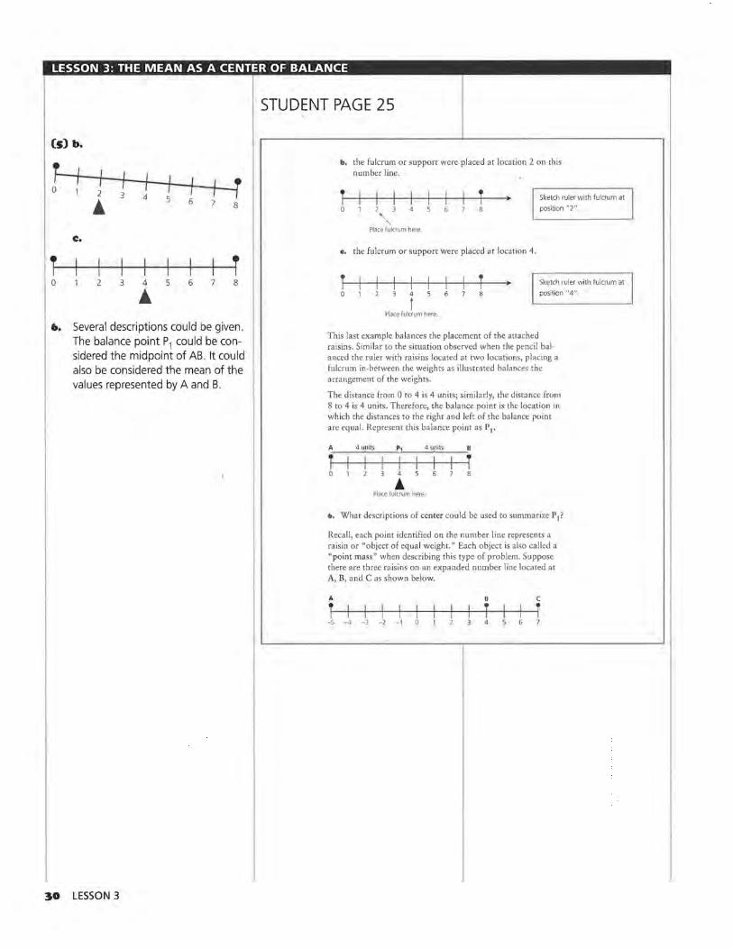
LESSON 3: THE MEAN AS A CENTER OF BALANCE
Csl b.
1- I I ( I ( ' 0 2 3 I l ----,
4 5 • 6 7 8
c.
T T 0 2 3 4 5 6 7 8 • 6. Several descriptions could be given.
The balance point P1 could be con-sidered the midpoint of AB. It could also be considered the mean of the values represented by A and B.
30 LESSON 3
STUDENT PAGE 25
b, the fulcrum or support were placed at location 2 on this number line.
T I I 0 2 3 4
"' Place fulcrum here,
T 6 8 I
Sketch ruler with fulcrum at I position "2"
e. the fulcrum or support were placed at location 4.
T 4
t Place fulcrum here.
T I
Sketch ruler with fulcrum at I position "4" .
This last example balances the placement of the attached raisins. Similar to the situation observed when the pencil balanced the ruler with raisins located at two locations, placing a fulcrum in-between the weights as illustrated balances the arrangement of the weights.
The distance from 0 to 4 is 4 units; similarly, the distance from 8 to 4 is 4 units. Therefore, the balance point is the location in which the distances to the right and left of the balance point are equal. Represent this balance point as Pt.
A 4unilt pl 4 ~nil>
T I T 0 4 8 • Place fulcrum here
to. What descriptions of center could be used to summarize P 1?
Recall, each point identified on the number line represents a raisin or "object of equal weight." Each object is also called a "point mass" when describing this type of problem. Suppose there are three raisins on an expanded number line located at A, B, and C as shown below.
A B c
T T I T -5 -4 -3 -2 - t 4 s
LESSON 3: THE MEAN AS A CENTER OF BALANCE
7. At this point in the lesson, it is not expected the students will know the mean is the balance point. This problem (along with Problems 8 and 9) are developing that summary. For this problem, a placement of the fulcrum at any location that gives more "weight" to the points B and C is considered appropriate. As will be shown later, the balance point for this arrangement is 2. Therefore, placing the fulcrum at any location less than 2 will produce this type of imbalance.
This same effect will be observed for any value less than 2. Consider the answer appropriate if the fulcrum is placed at any location less than 2.
8. For the imbalance to produce the opposite effect, the fulcrum can be placed at any location greater than 2. Moving the fulcrum in that position gives the weight at location A the illustrated imbalance.
Again, there could be several locations of the fulcrum that could produce the effect illustrated above. Consider any of the locations closer to the weights at B and C as appropriate.
9. Answers will vary. The precision to calculate this balance point will be developed later in the lesson. Therefore, locations close to 2 should be considered appropriate.
STUDENT PAGE 26
(Again, assume the number line is weightless. Obviously the ruler you used to demonstrate this model had weight and contributed to the location of the balance point. As the weight of the ruler is uniformly distributed, the weight and position of the raisins along the ruler essentially determine the balance point of each model. )
7. Where could the fulcrum be placed to produce the following sketch of the number line?
A
t- 1 I I I -s-~_11 I
-2 - I
I I 0
I I 2
I I 3
B
T 4
c
1--i 6 7
There could be several locations of the fulcrum that could produce the effect as illustrated by the above sketch. Copy the above sketch and shade the possible locations of the fulcrum that would result in the lack of balance as illustrated. Try modeling this sketch with a ruler and three raisins.
8. Where could the fulcrum be placed to produce the imbalance as illustrated in the following diagram?
c B !1--i I I ~ I A I I I \ G 7 t- I
I 5 I I I l 3 A
I -1 0 I -z - 5 -4 -3
Again, there could be several locations of the fulcrum that could produce the effect illustrated above. Copy the above sketch and shade the locations of the fulcrum that would result in the above imbalance of the number line. Also, experiment with a ruler and raisins to test your estimates.
9. Before you calculate the location of the fulcrum that would balance the three raisins, estimate where you would place the fulcrum to balance the model shown below.
A B c
T I I I I I T T -5 -4 -3 -2 -1 0 4
THE MEAN AS A CENTER OF BALANCE 31
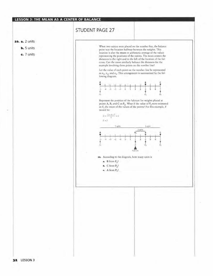
LESSON 3: THE MEAN AS A CENTER OF BALANCE
1.0. a. 2 units
b. 5 units
c:. 7 units
32 LESSON 3
STUDENT PAGE 27
When two raisins were placed on the number line, the balance point was the location halfway between the weights. This location is also the mean or arithmetic average of the values representing the positions of the raisins. The mean centers the distances to the right and to the left of the location of the fulcrum. Can the mean similarly balance the distances for the example involving three points on the number line?
Let the value of each point on the number line be represented as x 1, x 2, and x3' This arrangement is summarized by the following diagram.
A B c
T I t I 1 - 5 - 4 - 3 -2 - 1 4 6 7
t t t x, x, x,
Represent the position of the fulcrum for weights placed at points A, B, and C as P2. What if the value of P2 were estimated as x, the mean of the values of the points? For this example, x would be:
A
T - 5
t x,
x = - 5 + 4 + 7 = 2 3
7 units
I I I
- 4 - 3 -2 - 1
5 uni ts
~ P2 B
I t 2 4
t t x x, • fukrum
10. According to the diagram, how many units is
a. B from P2 ?
b . C from P2 ?
c . A from P2?
c
1 7
t x,
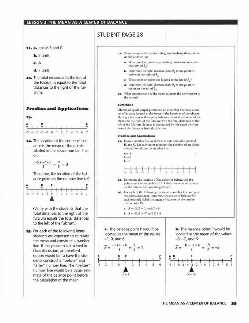
LESSON 3: THE MEAN AS A CENTER OF BALANCE
1.1.. a. points B and C
b. 7 units
c. A
d. 7 units
1.z. The total distances to the left of the fulcrum is equal to the total distances to the right of the fulcrum.
Practice and Applications
A B c T l r
-5 --4 -3 -2 -1 0 2 3 4 5 6 7
1.4. The location of the center of balance is the mean of the points labeled in the above number line, or:
-5 + -2 + 7 - _Q_ - 0 3 - 3 -
Therefore, the location of the balance point on the number line is 0:
A B P c T T I T
-5 --4 -3 -2 -1 0 234567 • (Verify with the students that the total distances to the right of the fulcrum equals the total distances to the left of the fulcrum.)
1.5. For each of the following items, students are expected to calculate the mean and construct a number line. If this problem is involved in class discussion, an excellent option would be to have the students construct a "before" and "after" number line. The "before" number line would be a visual estimate of the balance point before the calculation of the mean.
STUDENT PAGE 28
A
T -3
11. Examine again the previous diagram involving three points on the number line.
a. What point or points representing raisins are located to the right of P 2?
b. Determine the total distance from P2 to the point or points to the right of P2•
c. What point or points are located to the left of P 2?
d. Determine the total distance from P2 to the point or points to the left of P 2•
:az. What characteristic of the mean balances the distribution of the raisins?
SUMMARY
Objects of equal weight positioned on a number line have a center of balance located at the mean of the locations of the objects. Placing a fulcrum at this center balances the total distances of the objects to the right of the fulcrum with the total distances to the left of the fulcrum. Balance is maintained by this equal distribution of the distances from the fulcrum.
Practice and Applications
13. Draw a number line as shown. Locate and label points A, B, and C. Let each point represent the position of an object of equal weight on the number line.
A=-5
B =-2 (=7
-5 -4 -3 -2 -1 4
14. Determine the location of the center of balance for the points specified in problem 13. Label the center of balance on the number line you designed as P.
15. For each of the following, construct a number line and plot the points indicated. Determine the center of balance for each example (label the center of balance on the number line as point P).
a. A = -3, B = 0, and C = 6
b. A= -8, B = -7, and C = 6
a. The balance point P would be located as the mean of the values -3, 0, and 6:
b. The balance point P would be located as the mean of the values -8, -7, and 6:
-3 + 0 + 6 3 X= 3 =3=1
-8 +-7 + 6 -9 x = 3 = 3 =-3
B p c A B p c T I r T T I I I I I I I I I I l
-2 -1 0 1 2 3 4 5 6 -8 -7 -6 -5 --4 -3 -2 -1 0 1 2 3 4 5 6 • • X= 1 X=-3
THE MEAN AS A CENTER OF BALANCE 33
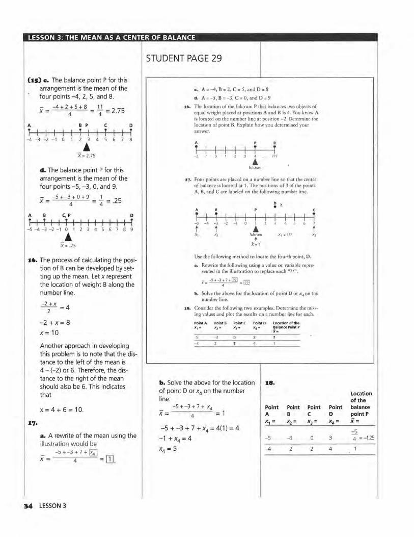
LESSON 3: THE MEAN AS A CENTER OF BALANCE
(J.S) c. The balance point P for this arrangement is the mean of the four points -4, 2, 5, and 8.
x = -4 + 2: 5 + 8 = ~ = 2.75
A B p c 0
T T I T T --4 -3 -2 -1 0 2 3 4 5 6 7 8
A
• X= 2.75
d. The balance point P for this arrangement is the mean of the four points -5, -3, 0, and 9.
- - 5 + -3 + 0 + 9 ..!_ 25 X= 4 =4=·
B C,P 0
T I T I T I I I I I I I I T -5 -4 -3 -2 -1 0 1 2 3 4 5 6 7 8 9 • X= .25
16. The process of calculating the position of B can be developed by set~ ting up the mean. Let x represent the location of weight B along the number line.
-2 +x = 4 2
-2 + x = 8
X=10
Another approach in developing this problem is to note that the distance to the left of the mean is 4 - (-2) or 6. Therefore, the distance to the right of the mean should also be 6. This indicates that
x = 4 + 6 = 10.
a. A rewrite of the mean using the illustration would be
-5+-3 + 7 + ~
x= 4 =OJ.
34 LESSON 3
STUDENT PAGE 29
c, A= -4, B = 2, C = 5, and D = 8
d. A= -5, B = -3, C = 0, and D = 9
16. The lo~ation of the fulcrum P that balances two objects of equal weight placed at positions A and B is 4. You know A is located on the number line at position -2. Determine the location of point B. Explain how you determined your answer.
A p B
t I f 1 -2 _,
4 '" • fulcrum
17. Four points are placed on a number line so that the center of balance is located at L The positions of 3 of the points A, B, and Care labeled on the following number line.
A e
1 I t I -5 -4 - J - 2 _, t t x, x,
p
I , • fulcrum
+ X=1
D
•
X4=?ll
c
1 7
t X3
Use the following method to locate the fourth point, D.
•· Rewrite the following using a value or variable represented in the illustration to replace each "??''.
ii'= -5 + -3 + 7 + ill] = "71 4 L'.D
b. Solve the above for the location of point Dor x4 on the number line.
18. Consider the following two examples. Determine the missing values and plot the results on a number line for each.
Point A Point B Point C PointD Location of the x, = X2= X3 = X4= Balance Point P X=
- 5 - 3 0 -4 1
b. Solve the above for the location 18. of point D or x4 on the number line.
~5 +-3 + 7 + x4 Point Point Point X= 4 = 1 A B c
x, = X2 = X3 = -5 + -3 + 7 + x4 = 4( 1) = 4
-1 +x4 = 4 - 5 -3 0
x4 = 5 --4 2 2
Location of the
Point balance D point P X4= x=
-5 3 4 = - 1.25
4
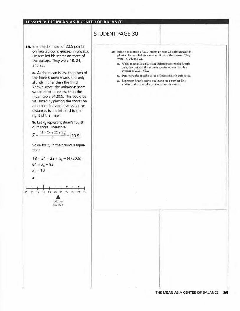
LESSON 3: THE MEAN AS A CENTER OF BALANCE
1.9. Brian had a mean of 20.5 points on four 25-point quizzes in physics. He recalled his scores on three of the quizzes. They were 18, 24,
15
and 22.
a. As the mean is less than two of the three known scores and only slightly higher than the third known score, the unknown score would need to be less than the mean score of 20.5. This could be visualized by placing the scores on a number line and discussing the distances to the left and to the right of the mean.
b. Let x4 represent Brian's fourth quiz score. Therefore:
- 18 + 24 + 22 + [;9 ~ X= 4 -=~
Solve for x4 in the previous equation:
18 + 24 + 22 + X4 = (4)(20.5)
64 + x4 = 82
x4 = 18
c.
• T I I T T
16 17 18 19 20 21 22 23 24
! fulcrum X= 20.5
25
STUDENT PAGE 30
19. Brian had a mean of 20.5 points on four 25-point quizzes in physics. He recalled his scores on three of the quizzes. They were 18, 24, and 22.
a. Without actually calculating Brian's score on the fourth quiz, determine if this score is greater or less than his average of 20.5. Why?
b. Determine the specific value of Brian's fourth quiz score.
"· Represent Brian's scores and mean on a number line similar to the examples presented in this lesson.
THE MEAN AS A CENTER OF BALANCE 35
LESSON 4
Weighted Averages Materials: Unit II Quiz
Technology: graphing calculator
Pacing: 2 class sessions
Overview
This lesson introduces some rather familiar problems involving weighted averages. The goal is to connect each example to a center of balance on a number line as introduced in Lesson 3. This provides a new look to some familiar problems. Some students will find this connection interesting; other students might find the presentation of average as a center of balance more difficult.
The interpretation of a weighted mean as a center is used in several of the lessons of this module. The variety of problems is intended to demonstrate the importance of a center. The representation of a balance point as derived from a weighted mean is quickly expanded to two-dimensional models in the latter lessons of this module.
Teaching Notes
This lesson was considered challenging by the fieldtest teachers. The difficulty noted by teachers was not in the type of problems but in the new organization of the information. This lesson is designed to assist in illustrating several examples involving the location of weights (or raisins) on a number line. Connecting the representation of test scores to the raisins used in Lesson 3 (or, similarly, the number of two-point baskets in basketball to the number of raisins) is intended to emphasize the mean as a center of balance.
:J6 LESSON 4
Technology
The use of the List options of many graphing calculators is growing in importance with this lesson. Although not necessary, it is possible to view the data presented in this lesson using the lists available on a graphing calculator. It is also possible to develop presentations of the problems through a spreadsheet application on a computer. Determining whether or not to consider these options should be based on the technology available and the timetable decided upon for this lesson. Each of these extensions would of
' course, add to the preparation and the pace of the lessons.
Follow· Up
The problems presented in this lesson could easily have been expanded. Quiz or test scores, sports data, weights on a balance, and so forth, are available and could be used as further investigations of the lesson. A simple data collection representing the number of hours students in a class watched television the previous day, or the number of brothers or sisters each student has, or the number of books read during a specific period of time, could be used to determine a class average by the methods described in this lesson.
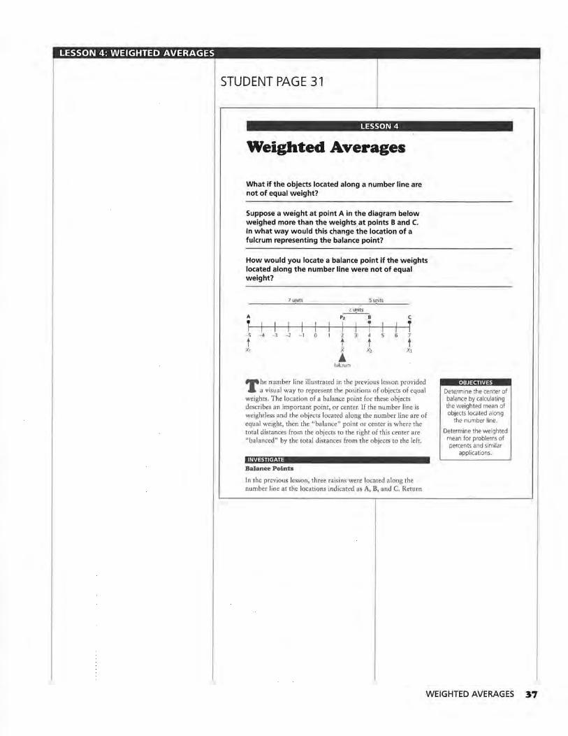
LESSON 4: WEIGHTED AVERAGES
STUDENT PAGE 31
LESSON 4
Weighted Averages
What if the objects located along a number line are not of equal weight?
Suppose a weight at point A in the diagram below weighed more than the weights at points B and C. In what way would this change the location of a fulcrum representing the balance point?
How would you locate a balance point if the weights located along the number line were not of equal weight?
7 ~nlu 5~1u
21..mils A p~ c
1 I I I t I I i -5 -4 -3 -2 -1 0 2 3 4 5 6 7
t t t t x, x x, x, • fulcrum
T he number line illustrated in the previous lesson provided a visual way to represent the positions of objects of equal
weights. The location of a balance point for these objects describes an important point, or center. If the number line is weightless and the objects located along the number line are of equal weight, then the "balance" point or center is where the total distances from the objects to the right of this center are "balanced" by the total distances from the objects to the left.
INVESTIGATE
Balance Points
In the previous lesson, three raisins were located along the number line at the locations indicated as A, B, and C. Return
Determine the center of balance by calculating the weighted mean of objects located along
the number line.
Determine the weighted mean for problems of percents and similar
applications.
WEIGHTED AVERAGES 37
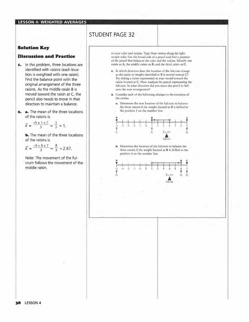
LESSON 4: WEIGHTED AVERAGES
Solution Key
Discussion and Praetiee
1. In this problem, three locations are identified with raisins (each location is weighted with one raisin). Find the balance point with the original arrangement of the three raisins. As the middle raisin B is moved toward the raisin at C, the pencil also needs to move in that direction to maintain a balance.
z. a. The mean of the three locations of the raisins is
X= -5 + 1 + 7
3 3
= 3=1.
b. The mean of the three locations of the raisins is
X= -5 + 6 + 7
3 8
= 3 ""2.67.
Note: The movement of the ful-. crum follows the movement of the middle raisin.
38 LESSON 4
STUDENT PAGE 32
to your ruler and raisins. Tape three raisins along the lightweight ruler. Use the broad side of a pencil and find a position of the pencil that balances the ruler and the raisins. Ident.ify one raisin as A, the middle raisin as B, and the third raisin as C.
J:, In which direction does the location of the fulcrum change as the raisin or weight identified at B is moved toward C? Try sliding a raisin represented in your model toward the raisin located at C. Now readjust the pencil representing the fulcrum. In what direction did you move the pencil to balance the new arrangement?
~. Consider each of the following changes to the locations of the raisins.
a, Determine the new location of the fulcrum to balance the three raisins if the weight located at B is shifted to the position 1 on the number line.
A e c
1 I r I t 1 -5 - 4 -3 - 2 -1 I 2 7
t t X= ???
t x, x, x, • fulcrum
b. Determine the location of the fulcrum to balance the three raisins if the weight located at B is shifted to the position 6 on the number line.
A B c
1 I t I I . t 1 -5 -4 -3 - 2 - I 4 s 6 7
t t t x, X =??? x, x, • fulcrum
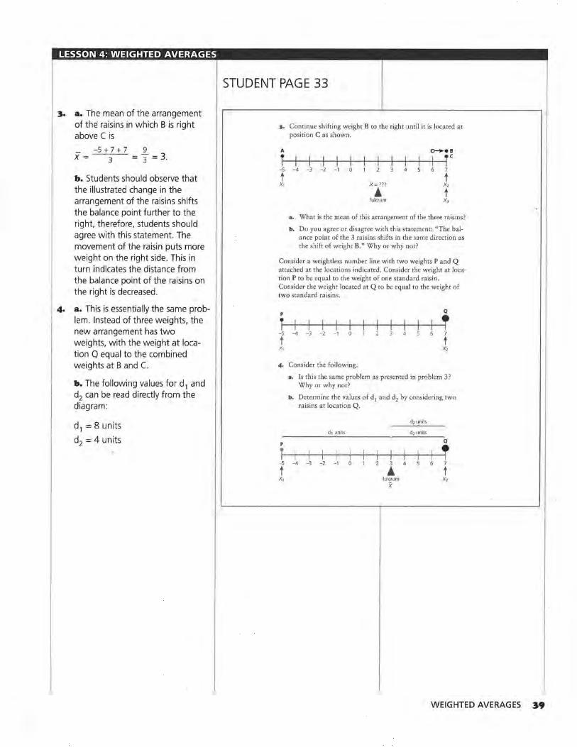
LESSON 4: WEIGHTED AVERAGES
~. a. The mean of the arrangement of the raisins in which B is right above C is
X= -5 + 7 + 7
3 9
= 3 = 3.
b. Students should observe that the illustrated change in the arrangement of the raisins shifts the balance point further to the right, therefore, students should agree with this statement. The movement of the raisin puts more weight on the right side. This in turn indicates the distance from the balance point of the raisins on the right is decreased.
4. a. This is essentially the same problem. Instead of three weights, the new arrangement has two weights, with the weight at location Q equal to the combined weights at B and C.
b. The following values for d1 and d2 can be read directly from the diagram:
d1 = 8 units
d2 = 4 units
STUDENT PAGE 33
3. Continue shifting weight B to the right until it is located at position C as shown.
A
T -5
t x,
o-+eB
I I I r -4 -3 -2 -1 7
t X= ??? x, • t fulcrum x,
a. What is the mean of this arrangement of the three raisins?
b. Do you agree or disagree with this statement: "The balance point of the 3 raisins shifts in the same direction as the shift of weight B." Why or why not?
Consider a weightless number line with two weights P and Q attached at the locations indicated. Consider the weight at location P to be equal to the weight of one standard raisin. Consider the weight located at Q to be equal to the weight of two standard raisins.
p
T -5
t x,
4.
p
T -5
t x,
Q
I I I T -4 -3 -2 -1 0 4 7
t x,
Consider the following.
a. Is this the same problem as presented in problem 3? Why or why not?
b. Determine the values of d1 and d2 by considering two raisins at location Q.
di units
d, units d2 units
Q
I T I -4 -3 -2 -1 3 4 7
A t fulcrum x,
x
WEIGHTED AVERAGES 39
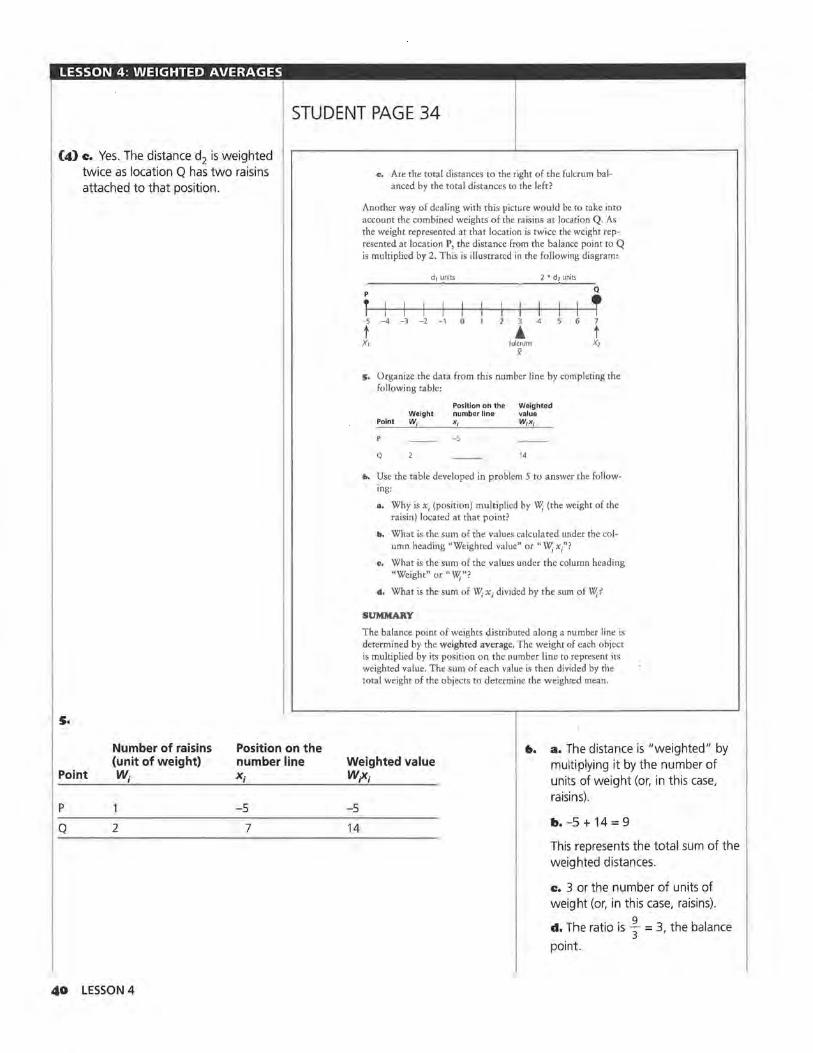
LESSON 4: WEIGHTED AVERAGES
STUDENT PAGE 34
(4) e. Yes. The distance d2 is weighted twice as location Q has two raisins attached to that position .
s.
Number of raisins Position on the (unit of weight) number line
Point W; X;
p -5
Q 2 7
40 LESSON 4
'" Are the total distances to the right of the fulcrum balanced by the total distances to the left?
Another way of dealing with this picture would be to take into account the combined weights of the raisins at location Q. As the weight represented at that location is twice the weight represented at location P, the distance from the balance point to Q is multiplied by 2. This is illustrated in the following diagram:
d1 units 2 • d2 units
p Q
1 I I I ~ - 5 -4 -3 -2 -1 0 3 5 6 7
t • t x, fulcrum x,
x
s. Organize the data from this number line by completing the following table:
Position on the Weighted Weight number line value
Point w. x1 W1x;
-5
Q 14
to. Use the table developed in problem 5 to answer the following:
a. Why is X; (position) multiplied by W; (the weight of the raisin) located at that point?
b. What is the sum of the values calculated under the column heading "Weighted value" or "W;x;''?
c. What is the sum of the values under the column heading "Weight" or "W;"?
d. What is the sum of W; X; divided by the sum of W;?
SUMMARY
The balance point of weights distributed along a number line is determined by the weighted average. The weight of each object is multiplied by its position on the number line to represent its weighted value. The sum of each value is then divided by the total weight of the objects to determine the weighted mean.
Weighted value 6. a. The distance is "weighted" by
multiplying it by the number of units of weight (or, in this case, raisins).
W;X;
-5
14 b. -5 + 14 = 9
This represents the total sum of the weighted distances.
e. 3 or the number of units of weight (or, in this case, raisins).
d. The ratio is f = 3, the balance
point.
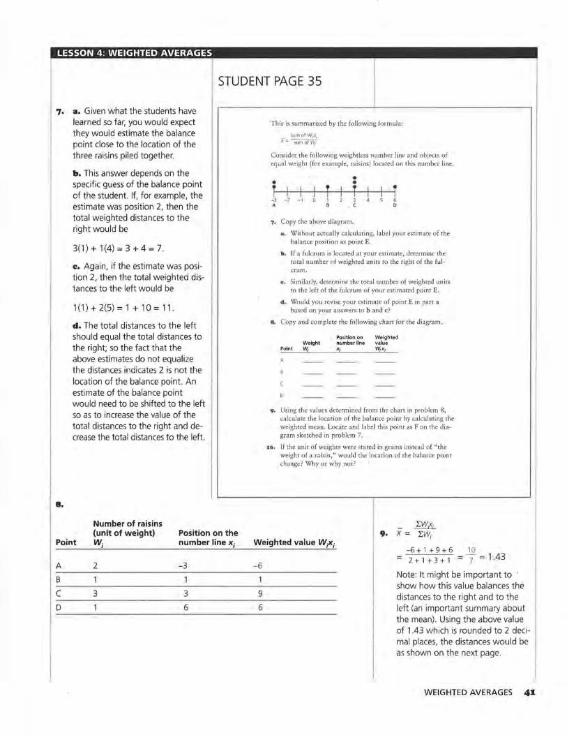
LESSON 4: WEIGHTED AVERAGES
STUDENT PAGE 35
7. a. Given what the students have learned so far, you would expect they would estimate the balance point close to the location of the three raisins piled together.
8.
b. This answer depends on the specific guess of the balance point of the student. If, for example, the estimate was position 2, then the total weighted distances to the right would be
3(1)+ 1(4)=3+4=7.
c. Again, if the estimate was position 2, then the total weighted distances to the left would be
1 (1) + 2(5) = 1 + 10 = 11 .
d. The total distances to the left should equal the total distances to the right; so the fact that the above estimates do not equalize the distances indicates 2 is not the location of the balance point. An estimate of the balance point would need to be shifted to the left so as to increase the value of the total distances to the right and decrease the total distances to the left.
Number of raisins (unit of weight) Position on the
Point W; number line X;
A 2 -3
B 1 1
c 3 3
D 6
This is summarized by the following formula:
sum of W,x,. X = sum of W;
Consider. the following weightless number line and objects of equal weight (for example, raisins) located on this number line.
• • • T I I T T T -3 - 2 -1 A
3 c
6 D
7. Copy the above diagram.
a. Without actually calculating, label your estimate of the balance position as point E.
b. If a fulcrum is located at your estimate, determine the total number of weighted units to the right of the fulcrum.
c. Similarly, determine the total number of weighted units to the left of the fulcrum of your estimated point E.
d. Would you revise your estimate of point E in part a based on your answers to b and c?
8. Copy and complete the following chart for the diagram.
Position on Weighted Weight number line value
Point w. x W;x1
A
c
D
9. Using the values determined from the chart in problem 8, calculate the location of the balance point by calculating the weighted mean. Locate and label this point as Fon the diagram sketched in problem 7.
:io. If the unit of weights were stated in grams instead of "the weight of a raisin," would the location of the balance point change? Why or why not?
Weighted value W;X;
:EWf; 9. X = :EW;
-6 + 1 +9+6 10
-6
9
6
= 2 + 1 + 3 + 1 = 7 "" 1 .43
Note: It might be important to show how this value balances the distances to the right and to the left (an important summary about the mean). Using the above value of 1.43 which is rounded to 2 decimal places, the distances would be as shown on the next page.
WEIGHTED AVERAGES 4I
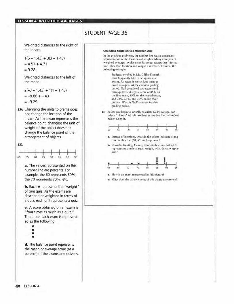
LESSON 4: WEIGHTED AVERAGES
Weighted distances to the right of the mean:
1 (6 - 1.43) + 3(3 - 1.43)
= 4.57 + 4.71
= 9.28.
Weighted distances to the left of the mean:
2(-3 - 1.43) + 1 (1 - 1 .43)
= -8.86 + -.43
=-9.29.
10. Changing the units to grams does not change the location of the mean. As the mean represents the balance point, changing the unit of weight of the object does not change the balance point of the arrangement of objects.
11.
60 65 70 75 80 85 90 95
a. The values represented on this number line are percents. For example, the 60 represents 60%, the 70 represents 70%, etc.
h. Each • represents the "weight" of one quiz. As the exams are de.scribed or weighted in terms of a quiz, each unit represents a quiz.
c. A score obtained on an exam is "four times as much as a quiz." Therefore, each exam is represented as the following :
• • • • d. The balance point represents the mean or average score (as a percent) of the exams and quizzes.
4Z LESSON 4
STUDENT PAGE 36
Changing Units on the Number Line
In the previous problems, the number line was a convenient representation of the locations of weights. Many examples of weighted averages involve a similar setup, except that information other than location and weight is involved. Consider the following example.
Students enrolled in Ms. Clifford's math class frequently take either quizzes or exams. An exam is worth four times as much as a quiz. At the end of a grading period, Gail completed two exams and three quizzes. She got a score of 85% on the first exam, 89% on the second exam, and 72%, 60%, and 76% on the three quizzes . What is Gail's average for this grading period?
11. Before you begin to actually calculate Gail's average, consider a "picture" of this problem. A number line is sketched below. Copy it.
60 65 70 75 80 85 90 95
a. Instead of locations, what do the values indicated along this number line (60, 65, etc.) represent?
b. Consider locating • along your number line. Instead of representing a unit of equal weight, what does a • represent?
• I • I• ' 60 65 70 75 80 85 9S
c. How is an exam represented in this picture?
d. What does the balance point of this diagram represent?
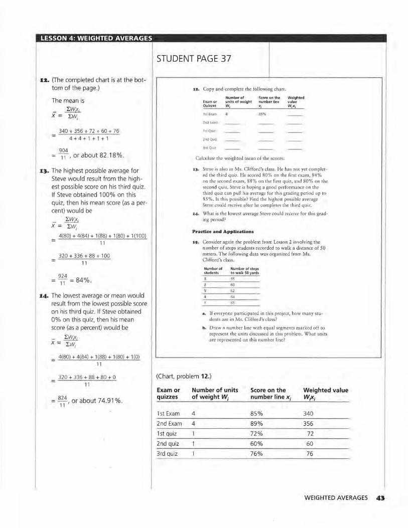
LESSON 4: WEIGHTED AVERAGES
12. (The completed chart is at the bottom of the page.)
The mean is
LW;X; X = LW;
340 + 356 + 72 + 60 + 76
4+4+1+1+1
904 =-1-1 ,orabout82.18%.
13. The highest possible average for Steve would result from the highest possible score on his third quiz. If Steve obtained 100% on this quiz, then his mean score (as a percent) would be
LW;X; X = LW;
4(80) + 4(84) + 1 (88) + 1 (80) + 1 ( 1 00)
11
320 + 336 + 88 + 100
11
924 = -1-1 = 84% .
14. The lowest average or mean would result from the lowest possible score on his third quiz. If Steve obtained 0% on this quiz, then his mean score (as a percent) would be
LW;X; X = LW;
= 4(80) + 4(84) + 1 (88) + 1 (80) + 1 (0)
11
320 + 336 + 88 + 80 + 0 = 11
= 824, or about 74.91 %.
11
STUDENT PAGE 37
x:z. Copy and complete the following chart.
Number of Score on the Weighted Exam or units of weight number line value Quizzes w. x,- W 1x1
1st Exam 85%
2nd Exam
1st Quiz
2nd Quiz
3rd Quiz
Calculate the weighted mean of the scores.
13. Steve is also in Ms. Clifford's class. He has not yet completed the third quiz. He scored 80% on the first exam, 84% on the second exam, 88% on the first quiz, and 80% on the second quiz. Steve is hoping a good performance on the third quiz can pull his average for this grading period up to 85%. ls this possible? Find the highest possible average Steve could receive after he completes the third quiz.
:14. What is the lowest average Steve could receive for this grading period?
Practice and Applications
:15, Consider again the problem from Lesson 2 involving the number of steps students recorded to walk a distance of 50 meters. The following data was organized from Ms. Cli fford's class.
Number of Number of steps students to walk 50 yards
55
60
s 62
4 64
. I 65
a. If everyone participated in this project, how many students are in Ms. Clifford's class?
b. Draw a number line with equal segments marked off to represent the units discussed in this problem. What units are represented on this number line?
(Chart, problem 12.)
Exam or Number of units Score on the Weighted value quizzes of weight W; number line X; W,x;
1st Exam 4 85% 340
2nd Exam 4 89% 356
1st quiz 72% 72
2rid quiz 60% 60
3rd quiz 76% 76
WEIGHTED AVERAGES 43
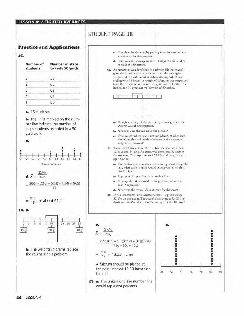
LESSON 4: WEIGHTED AVERAGES
Practice and Applications
15.
• • 1
Number of students
3
2
5
4
a. 1 5 students
Number of steps to walk 50 yards
55
60
62
64
65
b. The units marked on the number line indicate the number of steps students recorded in a 50-yard walk.
c.
• • • • • . • • T T T T
55 56 57 58 59 60 61 62 63 64 65
Number of steps
- l:W((; d. X = l:W;
- 3(55) + 2(60) + 5(62) + 4(64) + 1(65) - 15
916 = 15, or about 61.1
16. a.
0 3 6 9 12 15 1 21 24 27 30
otJ 12091 ~
b. The weights in grams replace the raisins in this problem.
44 LESSON 4
STUDENT PAGE 38
c.
c. Complete the drawing by placing •on the number line as indicated by this problem.
d. Determine the average number of steps this class rakes to walk the 50 meters.
:u.. An apparatus was developed in a physics lab that investigates the location of a balance point. A relatively lightweight rod was calibrated in inches, starting with 0 and ending with 30 inches. A weight of 15 grams was suspended from the 0 location of the rod, 20 grams at the location 15 inches, and 10 grams at the location of 30 inches.
, a, Complete a copy of this picture by showing where the
weights would be suspended.
b. What replaces the raisins in this picture?
c. If the weight of the rod is not considered, at what location along this rod would a balance of the suspended weights be obtained?
17; There are 26 students in Mr. Landwehr's Geometry class: 12 boys and 14 girls. An exam was completed by each of the students. The boys averaged 73.2 % and the girls averaged 80.5%.
a. If a number line were constructed to represent this problem, what scale or units would be represented on this number line?
b. Represent this problem on a number line.
c. If the symbol •was used in this problem, what does each • represent?
d. What was the overall class average for this exam?
18. In Ms. Mastromatteo's Geometry class, 12 girls average 82.1 % on this exam. The overall class average for 22 students was 84.4%. What was the average for the 10 boys?
b.
• = (15g)(Oin) + (20g)(15in) + (1 Og)(30in)
(15g + 20g + 10g)
• • • • 600 . h = 4s "' 13.33 inc es
A fulcrum should be placed at the point labeled 13.33 inches on the rod .
17. a. The units along the number line would represent percents.
70
• • • • • • • 72 74
• • • • • • • • • • • • • r 76 78 80 82
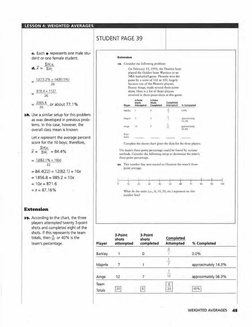
LESSON 4: WEIGHTED AVERAGES
c. Each • represents one male student or one female student.
~Wx.
d.x=~ I
=
=
12(73.2% + 14(80.5%)
26
878.4 + 1127
26
= 2005.4 , or about 77. 1 %
26
18. Use a similar setup for this problem as was developed in previous problems. In this case, however, the overall class mean is known.
Let x represent the average percent score for the 10 boys; therefore,
~W;X; X = ~W; = 84.4%
= 12(82.1 % + 1 O(x) 22
= 84.4(22) = 12(82.1) + 1 Ox
= 1856.8 = 985.2 + 1 Ox
= 1 Ox= 871.6
=X= 87 .16%
Extension
19. According to the chart, the three players attempted twenty 3-point shots and completed eight of the shots. If this represents the team totals, then 2~ or 40% is the
team's percentage.
STUDENT PAGE 39
Player
Barkley
Majerle
Ainge
Team
Totals
Extension
19. Consider the following problem:
On February 11, 1993, the Phoenix Suns played the Golden State Warriors in an NBA basketball game. Phoenix won the game by a score of 122 to 100, largely because one of the Phoenix players, Danny Ainge, made several three-point shots. Here is a list of those players involved in three-point shots at this game:
Player
Barkley
Majerle
Ainge
Team Totals
3-Polnt 3-Point Shots Shots Attempted Completed
12
Completed Attempted % Completed
0 0.0% 1
l approximately 7 14,3%
7 12 approximately
58,3%
Complete the above chart given the data for the three players.
The team's three-point percentage could be found by various methods. Consider th~ following setup to determine the team's three-point percentage.
20. This number line was started to illustrate the team's threepoint average.
I 0 10 20 30 40 50 60 70
What do the units (i.e., 0, 10, 20, etc.) represent on this number line?
3-Point 3-Point shots shots Com~leted
80 90
attempted completed Attempted % Completed
0
0 0.0%
100
7 7 approximately 14.3 %
7
12 7 12 approximately 58.3%
~ 0 I 280 I 14o%j
WEIGHTED AVERAGES 4S
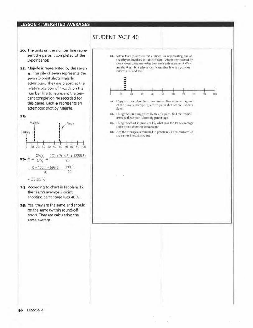
LESSON 4: WEIGHTED AVERAGES
::to. The un its on the number line represent the percent completed of the 3-point shots.
::&:l. Majerle is represented by the seven • . The pile of seven represents the seven 3-point shots Majerle attempted. They are placed at the relative position of 14.3 % on the number line to represent the percent completion he recorded for this game. Each • represents an attempted shot by Majerle.
::&::&.
Majerle i /Ainge i . Barkley • .
• . i • • . • • • • • T I • I I ·1 0 10 20 30 40 50 60 70 80 90 100
'LW;X; 1(0) + 7(14.3) + 12(58.3) ::&3. X = I:W = 20
I
0 + 100.1+699.6 799.7 = 20 20
""39.99%
::&4. According to chart in Problem 19, the team's average 3-point shooting percentage was 40%.
::ts. Yes, they are the same and should be the same (within round-off error) . They are calculating the same average.
46 LESSON 4
STUDENT PAGE 40
z1. Seven •are placed on this number line representing one of the players involved in this problem. Who is represented by these seven units and what does each unit represent? Why are the •symbols placed on the number line at a position between 10 and 20?
• • • • • I • I • 0 10 20 30 40 so 60 70 80
zz. Copy and complete the above number line representing each of the players attempting a three-point shot for the Phoenix Suns.
ZJ. Using the setup suggested by this diagram, find the team's average three-point shooting percentage.
z4, Using the chart in problem i9, what was the team's average three-point shooting percentage?
zs. Are the averages determined in problem 23 and problem 24 the same? Should they be?
I 90 100

UNIT Ill
''Raisin'' Country

LESSON 5
Balancing a Point-Mass Triangle Materials: heavy paper, raisins, tape, Activity Sheet 4, Activity Sheet 7
Technology: graphing calculator Pacing: 2 class sessions
Overview
The major theme of this section continues to demonstrate mean as a center of balance. This lesson moves the number line and the previous one-dimensional representations of a balance point to the twodimensional models. This lesson specifically focuses on a triangle and the location of a balance point represented by a triangle's vertices. The triangles presented on the blackline masters for this lesson are cut out of heavier paper; raisins are taped to the vertices of each triangle. This represents the point-mass triangles described in this lesson. Point-mass problems consider the weighted objects (or raisins) as the defining characteristic of the shape. The point at which each triangle model balances on the end of a pencil is described as the balance point of that triangle. This point is compared to a centroid, or the coordinate point represented by the mean of the coordinates of the vertices.
This lesson develops another method in locating a balance point (for a point-mass model) by a process described as "collapsing the raisins." This process is used to demonstrate several properties of a triangle and is used in several of the lessons involving other geometric shapes presented in the lessons following a student's work with triangles.
Teaching Notes
The topics in this lesson are reinforced by the hands-on development of the point-mass models.
The triangle models will most dramatically indicate the connections of the balance point to the centroid and the collapsed point. For triangles, this point is also connected to the intersection of the medians. As the geometric figures expand to quadrilaterals and other polygons, the connection of the hands-on locations to the calculated points are not as apparent. This lesson, therefore, sets up important topics for several of the lessons involved in the remaining portions of this module. The development of the models to highlight the special properties and characteristics of triangles is important. If, however, it is not possible for every student to construct the paper-and-raisin models, a few of these models constructed by the teacher will be sufficient for solving the problems presented.
It is suggested the models be stored in a envelope for each student until the completion of Lesson 8 since each new lesson expands on the previous models.
Technology
This lesson could be used to introduce the LIST options of a graphing calculator. Specific directions for work with a graphing calculator are provided in Lesson 7 as the number of vertices and the number of raisins are expanded. A simple introduction using the triangle models is encouraged if this type of calculator work is new to the students. If a computer lab environment is available, you may want to represent the data as outlined in the lesson by using a spreadsheet application. Using either a graphing calculator or a spreadsheet (or both) is an excellent method to begin working with several new topics of center.
BALANCING A POINT-MASS TRIANGLE 49
LESSON 5: BALANCING A POINT-MASS TRIANGLE
SO LESSON 5
STUDENT PAGE 43
LESSON 5
Balancing a Point-Mass Triangle
Do you think there is a balance point for three points located on a plane?
If a balance point exists, how can you find it? Is there a model similar to the ruler, raisins, and pencil?
When might it be important to know this balance point?
B alancing equal weights on a number line involves finding a point or center that evenly distributes the total distances of
each weight to the left and to the right of the balance point. Expand this idea to three noncollinear points. Consider objects of equal weight located at three points on a sheet of paper.
INVESTIGATE
Balancing the Triangle
Triangles represent one of the most basic geometric shapes you will study. More complex geometric shapes are frequently investigated by dividing them into triangles! Triangles are described and classified by their angle measures and the lengths of their sides.
A triangle in which each of its three angles has a measure less than 90 degrees is called an acute triangle.
A triangle in which each all three sides are of equal length is called an equilateral triangle.
, , Determine the balance point of a point-mass triangle by experimen-
tation.
Determine the centroid of a point-mass triangle
Construct the intersection of the medians of a
triangle.
Summarize the relationship of balance point,
centroid, and intersection of medians.
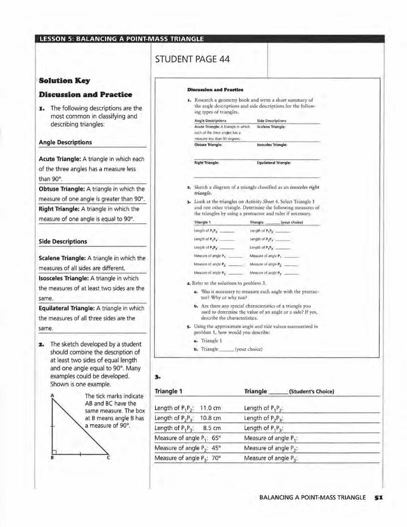
LESSON 5: BALANCING A POINT-MASS TRIANGLE
Solution Key
Discussion and Practice
1.. The following descriptions are the most common in classifying and describing triangles:
Angle Descriptions
Acute Triangle: A triangle in which each
of the three angles has a measure less
than go0•
Obtuse Triangle: A triangle in which the
measure of one angle is greater than go0•
Right Triangle: A triangle in which the
measure of one angle is equal to go0•
Side Descriptions
Scalene Triangle: A triangle in which the
measures of all sides are different.
Isosceles Triangle: A triangle in which
the measures of at least two sides are the
same.
Equilateral Triangle: A triangle in which
the measures of all three sides are the
same.
2. The sketch developed by a student should combine the description of at least two sides of equal length and one angle equal to 90°. Many examples could be developed. Shown is one example.
A
8
The tick marks indicate AB and BC have the same measure. The box at B means angle B has a measure of go0
•
c
STUDENT PAGE 44
Triangle 1
Dl•cu••lon and Practice
1. Research a geometry book and write a short summary of the angle descriptions and side descriptions for rhe following types of triangles.
Angle Descriptions Side Descriptions
Acute Triangle: A triangle in which Scalene Triangle:
each of the three angles has a measure less than 90 degrees
Obtuse ll'langle: Isosceles Triangle:
Right ll'langle: Equilateral Triangle:
a. Sketch a diagram of a triangle classified as an isosceles right triangle.
~ Look at the triangles on Activity Sheet 4. Select Triangle 1 and one other triangle. Determine the following measures of the triangles by using a protractor and ruler if necessary.
Trlangle 1
length of P1P2: __
Length of P2P3 : __
Length of P1P3: __
Triangle __ (your choice)
Length of P2P
3: __
length of P1P3: __
Measure of angle P1: __ Measure of angle P1:
Measure of angle P2: __ Measure of arigle P2: _ _
Measure of angle Pl: __ Measure of angle P3:
4, Refer to the solutions to problem 3.
a. Was it necessary to measure each angle with the protractor? Why or why not?
b. Are there any special characteristics of a triangle you used to determine the value of an angle or a side? If yes, describe the characteristics.
5. Using the approximate angle and side values summarized in problem l, how would you describe:
a. Triangle 1
b. Triangle __ (your choice)
Triangle ___ (Student's Choice)
Length of P,P2: 11 .0 cm
Length of P1P3: 8.5 cm
Measure of angle P 1: 65° Measure of angle P 1:
Measure of angle P2: 45° Measure of angle P2:
Measure of angle P3: 70° Measure of angle P3:
BALANCING A POINT-MASS TRIANGLE SI
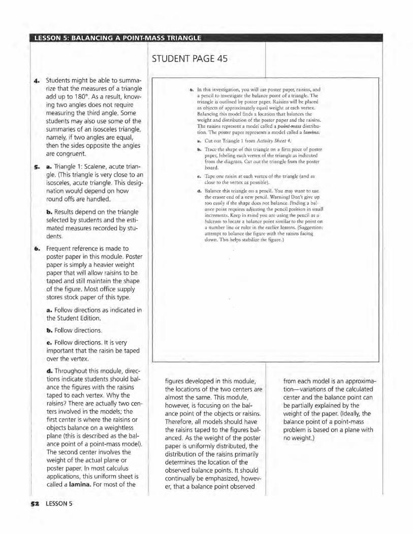
LESSON 5: BALANCING A POINT-MASS TRIANGLE
4. Students might be able to summa-rize that the measures of a triangle add up to 180°. As a result, know-ing two angles does not require measuring the third angle. Some students may also use some of the summaries of an isosceles triangle, namely, if two angles are equal, then the sides opposite the angles are congruent.
s. a. Triangle 1: Scalene, acute trian-gle. (This triangle is very close to an isosceles, acute triangle. This desig-nation would depend on how round offs are handled.
b. Results depend on the triangle selected by students and the esti-mated measures recorded by stu-dents.
6. Frequent reference is made to poster paper in this module. Poster paper is simply a heavier weight paper that will allow raisins to be taped and still maintain the shape of the figure. Most office supply stores stock paper of this type.
a. Follow directions as indicated in the Student Edition .
b. Follow directions.
c. Follow directions. It is very important that the raisin be taped over the vertex.
d. Throughout this module, di rec-tions indicate students should bal-ance the figures with the raisins taped to each vertex. Why the raisins? There are actually two cen-ters involved in the models; the first center is where the raisins or objects balance on a weightless plane (this is described as the bal-ance point of a point-mass model). The second center involves the weight of the actual plane or poster paper. In most calculus applications, this uniform sheet is called a lamina. For most of the
52 LESSON 5
STUDENT PAGE 45
t.. In this investigation, you will use poster paper, raisins, and a pencil to investigate the balance point of a triangle. The triangle is outlined by poster paper. Raisins will be placed as objects of approximately equal weight at each vertex. Balancing this model finds a location that balances the weight and distribution of the poster paper and the raisins. The raisins represent a model called a point-mass distribution. The poster pa per represents a model called a lamina.
a. Cut out Triangle 1 from Activity Sheet 4.
b. Trace the shape of this triangle on a firm piece of poster paper, labeling each vertex of the triangle as indicated from the diagram. Cut out the triangle from the poster board.
c. Tape one raisin at each vertex of the triangle (and as close to the vertex as possible).
d. Balance this triangle on a pencil. You may want to use the eraser end of a new pencil. Warning! Don't give up too easily if the shape does not balance. Finding a balance point requires adjusting the pencil position in small increments . Keep in mind you are using the pencil as a fulcrum to locate a balance point similar to the point on a number line or ruler in the earlier lessons. (Suggestion: attempt to bafance the figure with the raisins facing down. This helps stabilize the figure.)
figures developed in this module, the locations of the two centers are almost the same. This module, however, is focusing on the balance point of the objects or raisins. Therefore, all models should have the raisins taped to the figures balanced . As the weight of the poster paper is uniformly distributed, the distribution of the raisins primarily determines the location of the observed balance points. It should continually be emphasized, however, that a balance point observed
from each model is an approximation-variations of the calculated center and the balance point can be partially explained by the weight of the paper. (Ideally, the balance point of a point-mass problem is based on a plane with no weight.)
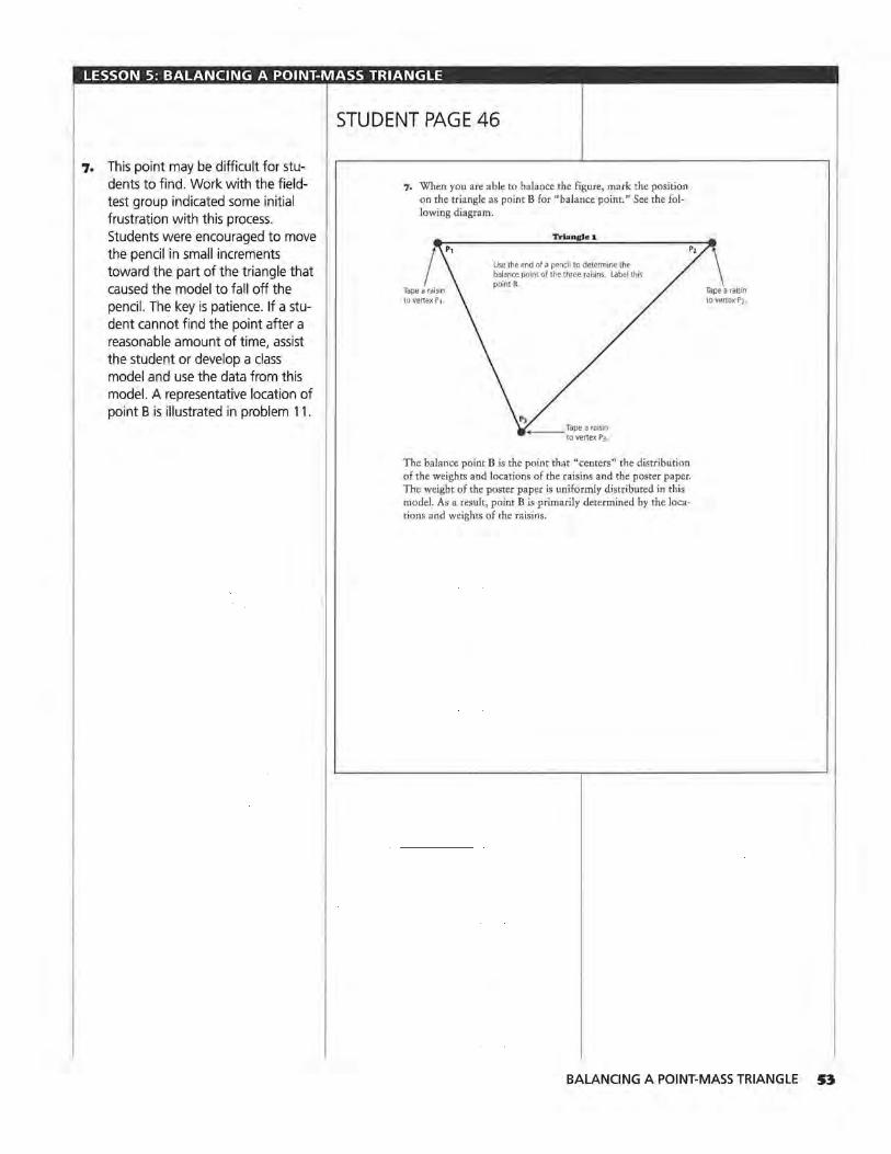
LESSON 5: BALANCING A POINT-MASS TRIANGLE
7. This point may be difficult for students to find. Work with the fieldtest group indicated some initial frustration with this process. Students were encouraged to move the pencil in small increments toward the part of the triangle that caused the model to fall off the pencil. The key is patience. If a student cannot find the point after a reasonable amount of time, assist the student or develop a class model and use the data from this model. A representative location of point B is illustrated in problem 11.
STUDENT PAGE 46
7. When you are able to balance the figure, mark the position on the triangle as point B for "balance point." See the following diagram.
Trlan11lc 1
Use the end of a pencil to determine the balance point of the three raisins Label this point B.
The balance point Bis the point that "centers" the distribution of the weights and locations of the raisins and the poster paper. The weight of the poster paper is uniformly distributed in this model. As a result, point B is primarily determined by the locations and weights of the raisins.
Tape a raisin to vertex P2.
BALANCING A POINT-MASS TRIANGLE 53
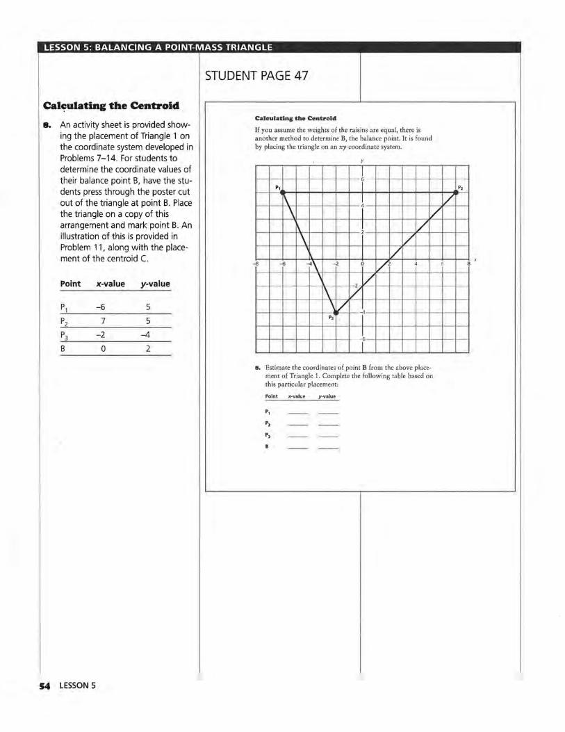
LESSON 5: BALANCING A POINT-MASS TRIANGLE
Calf?ulating the Centroid
8. An activity sheet is provided showing the placement of Triangle 1 on the coordinate system developed in Problems 7-14. For students to determine the coordinate values of their balance point B, have the students press through the poster cut out of the triangle at point B. Place the triangle on a copy of this arrangement and mark point B. An illustration of this is provided in Problem 11, along with the placement of the centroid C.
Point x-value y-value
P1 -6 5
Pz 7 5
P3 -2 -4
B 0 2
54 LESSON 5
STUDENT PAGE 47
Calculating the Centroid
If you assume the weights of the raisins are equal, there is another method to determine B, the balance point. It is found by placing the triangle on an xy-coordinate system.
y
I 6
P1 I \
t \ / \ I / \ I /
/ -8 -6 -4\ -2 0 / 2
' ~ \ t7 \V
-<I P3 I
I 6
I 11. Estimate the coordinates of point B from the above place
ment of Triangle 1. Complete the following table based on this particular placement:
Point x-value y-vatue
P2
I/
8
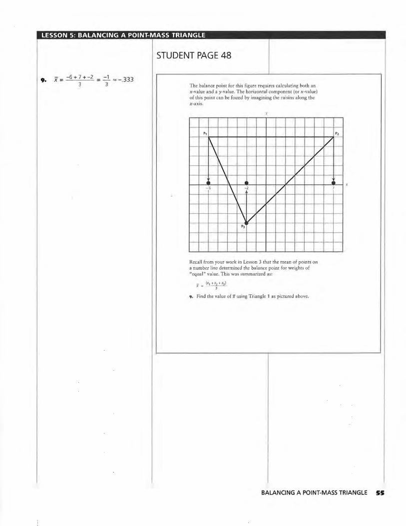
LESSON 5: BALANCING A POINT-MASS TRIANGLE
•• x = -6 + 7 + -2 = -=l ""-.333 3 3
STUDENT PAGE 48
The balance point for this figure requires calculating both an x-value and a y-value. The horizontal component (or x-value) of this point can be found by imagining the raisins along the x-axis.
y
P1
\ \ /
\ / \ / .. .. I/
-6 \ -2 i/ ' i/ \ i/
~
\V P3
Recall from your work in Lesson 3 that the mean of points on a number line determined the balance point for weights of "equal" value. This was summarized as:
X = (x,+xz+X3) 3
9. Find the value of x using Triangle 1 as pictured above.
P2
/
0
BALANCING A POINT-MASS TRIANGLE SS
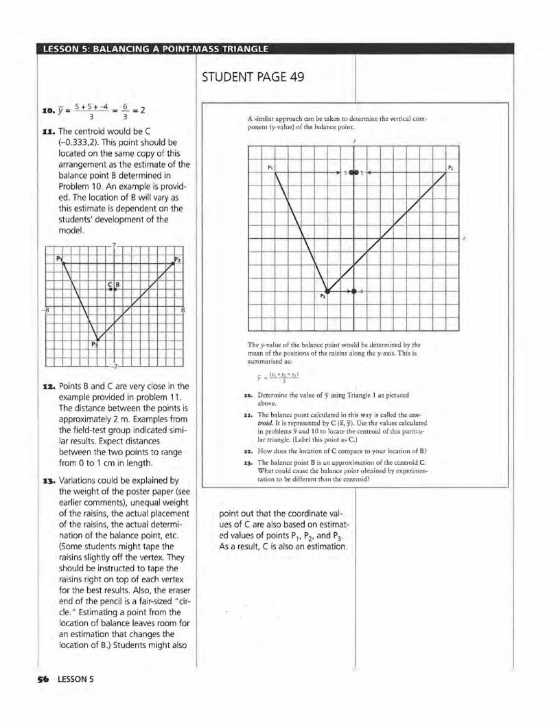
LESSON 5: BALANCING A POINT-MASS TRIANGLE
10. y = 5 + 5 + -4 = ~ = 2 3 3
11. The centroid would be C (--0.333,2). This point should be located on the same copy of this arrangement as the estimate of the balance point B determined in Problem 10. An example is provided. The location of B will vary as this estimate is dependent on the students' development of the model.
P1 Pz I\ v ' /
\ C B v \ - v
v -8 \ v
v \ v '/
p
7
1z. Points B and C are very close in the example provided in problem 11 . The distance between the points is approximately 2 m. Examples from the field-test group indicated similar results. Expect distances between the two points to range from 0 to 1 cm in length.
1~. Variations could be explained by the weight of the poster paper (see earlier comments), unequal weight of the raisins, the actual placement of the raisins, the actual determination of the balance point, etc. (Some students might tape the raisins slightly off the vertex. They should be instructed to tape the raisins right on top of each vertex for the best results. Also, the eraser end of the pencil is a fair-sized "circle." Estimating a point from the location of balance leaves room for an estimation that changes the location of B.) Students might also
S6 LESSON 5
STUDENT PAGE 49
A similar approach can be taken to determine the vertical component (y-value) of the balance point.
y
P1 SI •s
\ \
\ / \ /
\ / \ / ' / \ / \/
-4 P,
They-value of the balance point would be determined by the mean of the positions of the raisins along the y-axis. This is summarized as:
Y- - (y, +y,+y,)
- 3
10. Determine the value of y using Triangle 1 as pictured above.
/
u. The balance point calculated in this way is called the centroid. It is represented by C (x, y). Use the values calculated in problems 9 and 10 to locate the centroid of this particular triangle. (Label this point as C.)
n. How does the location of C compare to your location of B?
u. The balance point B is an approximation of the centroid C. What could cause the balance point obtained by experimentation to be different than the centroid?
point out that the coordinate values of C are also based on estimated values of points P1, P2, and P3.
As a result, C is also an estimation.
P2
/
x
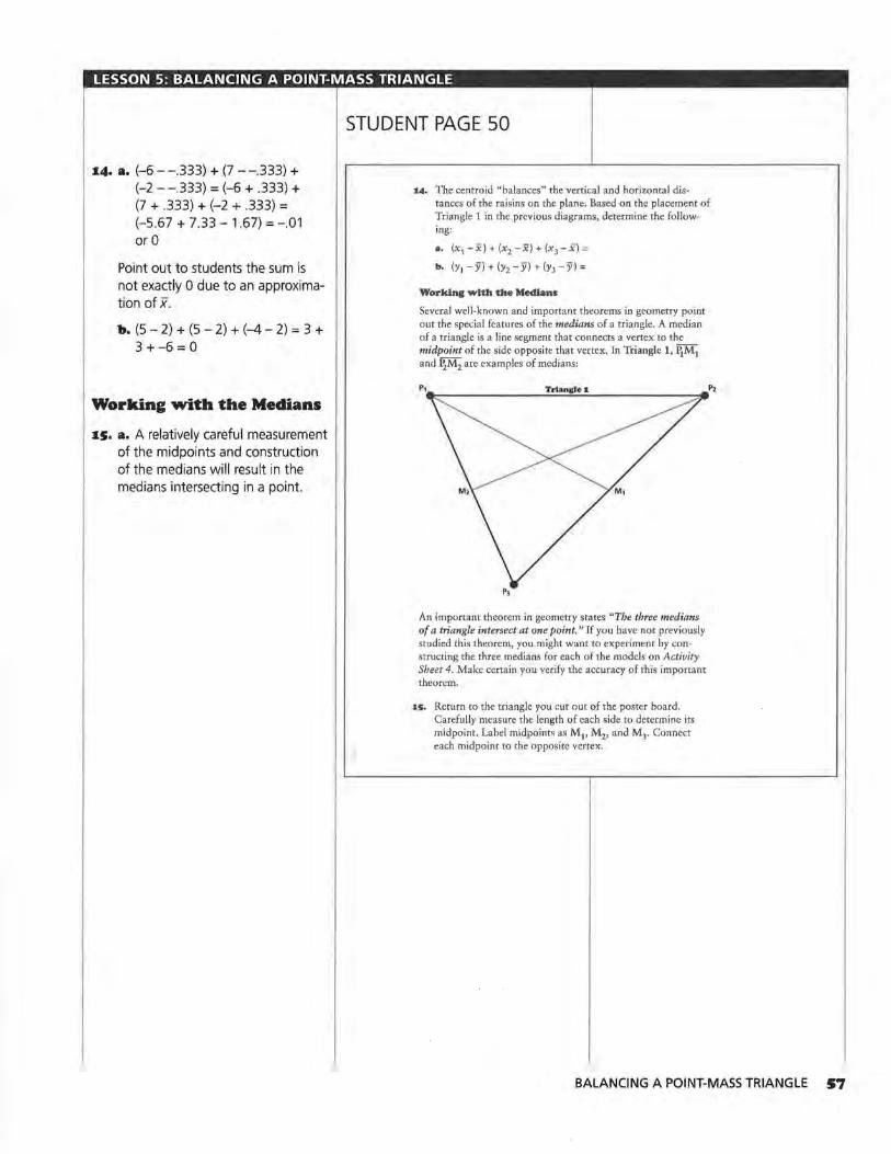
LESSON 5: BALANCING A POINT-MASS TRIANGLE
14. a. (-6 - -.333) + (7 - -.333) + (-2 - -.333) = (-6 + .333) + (7 + .333) + (-2 + .333) = (-5 .67 + 7.33 - 1.67) = - .01 or 0
Point out to students the sum is not exactly 0 due to an approximation of x. h. (5 - 2) + (5 - 2) + (-4 - 2) = 3 +
3+-6=0
Working with the Medians
15. a. A relatively careful measurement of the midpoints and construction of the medians will result in the medians intersecting in a point.
STUDENT PAGE 50
14, The centroid "balances" the vertical and horizontal distances of the raisins on the plane. Based on the placement of Triangle 1 in the previous diagrams, determine the following:
a. (xi - x) + (xz - x) + (x3 - x) =
b. (Y1 -Y) + (yz-Yl + (y3-Y) =
Working with the Medians
Several well-known and important theorems in geometry point out the special features of the medians of a triangle. A median of a triangle is a line segment that connects a vertex to the midpoint of the side opposite that vertex. In Triangle 1, P1M 1 and PzM2 are examples of medians:
An important theorem in geometry states "The three medians of a triangle intersect at one point." If you have not previously studied this theorem, you might want to experiment by constructing the three medians for each of the models on Activity Sheet 4. Make certain you verify the accuracy of this important theorem.
1s. Return to the triangle you cut out of the poster board. Carefully measure the length of each side to determine its midpoint. Label midpoints as Ml> M 2, and MJ" Connect each midpoint to the opposite vertex.
BALANCING A POINT-MASS TRIANGLE S7
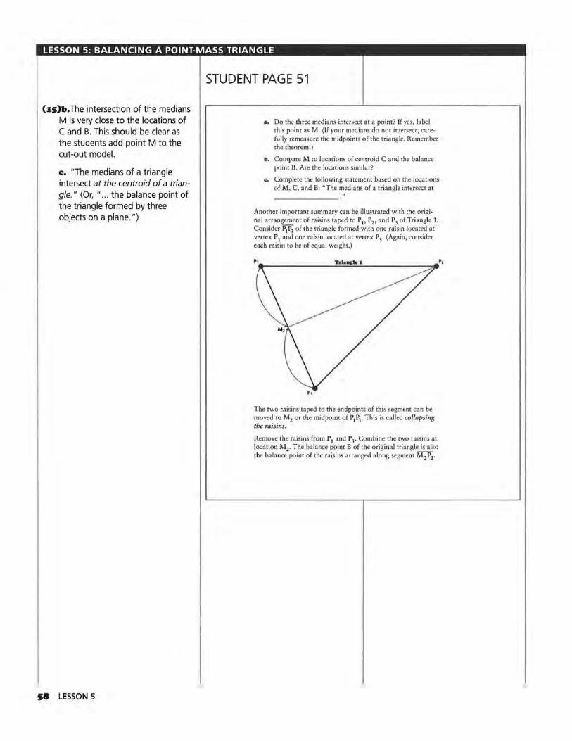
LESSON 5: BALANCING A POINT-MASS TRIANGLE
bs)b. The intersection of the medians M is very close to the locations of C and B. This should be clear as the students add point M to the cut-out model.
c. "The medians of a triangle intersect at the centroid of a triangle." (Or, " ... the balance point of the triangle formed by three objects on a plane.")
S8 LESSON 5
STUDENT PAGE 51
•· Do the three medians intersect at a point? If yes, label this point as M. (If your medians do not intersect, carefully remeasure the midpoints of the triangle. Remember the theorem!)
b. Compare M to locations of centroid C and the balance point B. Are the locations similar?
"' Complete the following statement based on the locations of M, C, and B: "The medians of a triangle intersect at
Another important summary can be illustrated with the original arrangement of raisins taped to P1, P2, and P3 of Triangle 1. Consider P1P3 of the triangle formed with one raisin located at vertex P 1 and one raisin located at vertex P 3' (Again, consider each raisin to be of equal weight.)
The two raisins taped to the endpoints of this segment can be moved to M2 or the midpoint of P1P3. This is called collapsing the raisins.
Remove the raisins from P1 and P3. Combine the two raisins at location M2. The balance point B of the original triangle is also the balance point of the raisins arranged along segment M 2 P2•
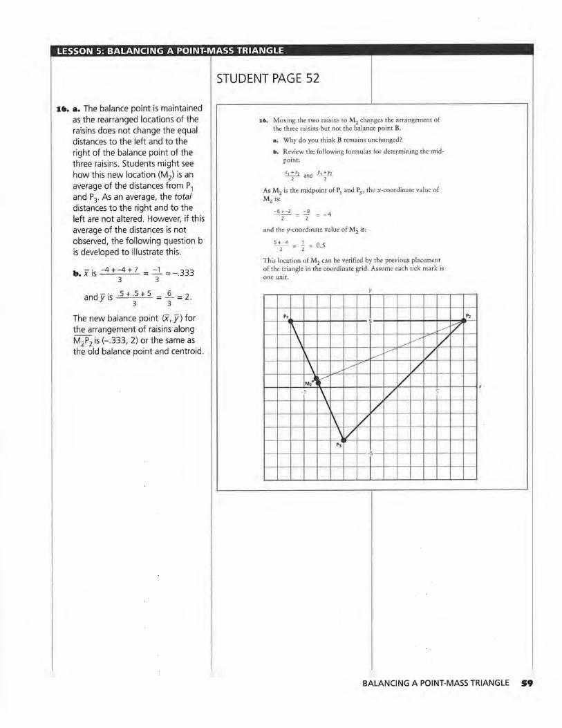
LESSON 5: BALANCING A POINT-MASS TRIANGLE
16. a. The balance point is maintained as the rearranged locations of the raisins does not change the equal distances to the left and to the right of the balance point of the three raisins. Students might see how this new location (M2) is an average of the distances from P1 and P3 . As an average, the total distances to the right and to the left are not altered. However, if this average of the distances is not observed, the following question b is developed to illustrate this.
b. x is --4 + - 4 + 7 = 2 "" -.333 3 3
and y is ·5 + ·5 + 5 = ~ = 2. 3 3
The new balance point (x, fl for the arrangement of raisins along M2P2 is (-.333, 2) or the same as the old balance point and centroid.
STUDENT PAGE 52
U•. Moving the two raisins to M2 changes the arrangement of the three raisins but not the balance point B.
a. Why do you think B remains unchanged?
b. Review the following formulas for determining the midpoint:
x, ;xz and Y1 ;ri As M 2 is the midpoint of P1 and P3 , the x-coordinate value of M 2 is:
-6+-2 = ~ = -4 2 2
and the y-coordinate value of M2 is:
5 +-4 = _1_ = 0.5 2 2
This location of M 2 can be verified by the previous placement of the triangle in the coordinate grid. Assume each tick mark is one unit.
y
P1 I ~
\ _V
\ ~ 7
/ __..-
:\. v v 7 \ _,,.v / 7
M,) r 7 -5 \ I/ 5
\ / \ / \ /
P3
I
P2
~
BALANCING A POINT-MASS TRIANGLE S9
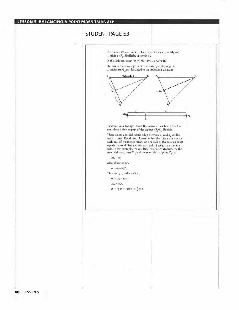
LESSON 5: BALANCING A POINT-MASS TRIANGLE
60 LESSON 5
STUDENT PAGE 53
Determine x based on the placement of 2 raisins at M 2 and 1 raisin at P2. Similarly, determine y.
Is this balance point ( x, f) the same as point B?
Return to the rearrangement of raisins by collapsing the 2 raisins to M 2 as illustrated in the following diagram:
Examine your triangle. Point B, discovered earlier in this lesson, should also be part of the segment P2M2. Explain.
There exists a special relationship between d1 and d2 as illustrated above. Recall from Lesson 4 that the total distances for each unit of weight (or raisin) on one side of the balance point equals the total distances for each unit of weight on the other side. In this example, the resulting balance contributed by the two raisins at point M2 and the one raisin at point P2 is:
2d, = ld,
Also observe that:
d1 + d2 = M2P2
Therefore, by substitution,
d1 + 2d1 = M2P2
3d1 = M2P2
d1 = t M2P2 and d2 = t M2P2
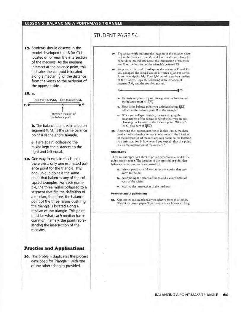
LESSON 5: BALANCING A POINT-MASS TRIANGLE
17. Students should observe in the model developed that B (or C) is located on or near the intersection of the medians. As the medians intersect at the balance point, this indicates the centroid is located along a median f of the distance from the vertex to the midpoint of the opposite side.
18. a.
Two-thirds of P1M1 One-third of P1M1
P,e---------ft'------M1
t Estimated location of the balance point
b. The balance point estimated on segment P1M 1 is the same balance point B of the entire triangle.
c:. Here again, collapsing the raisins kept the distances to the right and left equal.
19. One way to explain this is that there exists only one estimated balance point for the triangle. This one, unique point is the same point that balances any of the collapsed examples. For each example, the three raisins collapsed to a segment that fits the definition of a median, therefore, the balance point of the three raisins outlining the triangle is located along a median of the triangle. This point must be what each median has in common, namely, the point representing the intersection of the medians.
Practice and Applications
zo. This problem duplicates the process developed for Triangle 1 with one of the other triangles provided.
STUDENT PAGE 54
17. The above work indicates the location of the balance point is} of the distance from M2 and t of the distance from P2.
What does this indicate about the intersection of the medians M or the location of the triangle's centroid C?
18. Suppose that instead of collapsing the raisins at P1 and P2 you collapsed the raisins located at vertex P2 and at vertex P3 to the midpoint M 1. Then r;M;" would also be a median of the triangle. Copy the following representation of segment P1Mi and the attached raisins.
P1----------------.: M1
a. Estimate on your copy of this segment the location of the balance point of P1 Mi.
b. How is the balance point you estimated along P1Mi related to the balance point B of the triangle?
e. When you collapse raisins, you are changing the arrangement of the raisins or weights but you are not changing the location of the balance point. Why is B (or C) also part of Pi.Mi?
19. According the theorem mentioned in this lesson, the three medians of a triangle intersect in one point. If the location of the intersection of the medians was based on the location you estimated for B, how would you explain that this point is also the intersection of the medians?
SUMMARY
Three raisins taped to a sheet of poster paper form a model of a point-mass triangle. The location of the centroid or point that balances the raisins can be estimated by:
a. using a pencil as a fulcrum to locate a point that balances the model
b. determining the means of the x- and y-coordinates of each of the raisins
e. locating the intersection of the medians
Praetlee and Applleatlons
zo. Cut out the second triangle you selected from the Activity Sheet 4 on poster paper. Tape a raisin at each vertex. Using
BALANCING A POINT-MASS TRIANGLE ·~
LESSON 5: BALANCING A POINT-MASS TRIANGLE
STUDENT PAGE 55
21. Answers will vary dependent on students' arrangement of the cutout triangle on the coordinate grid . Emphasize that the placement of the triangle is not important. In other words, each student will have different coordinate values but the final location of the centroid within the triangle should be the same.
22. Results depend on the triangle selected and the estimates of the coordinate values for each vertex.
23. The location of C should be close to the student's estimate of the balance point B. This is similar to the process developed in Problems 14-19.
24. a. Students should conjecture that the points are the same.
b. Differences in the points are again related to varying weights in the raisins, estimating the center point from the pencil, specific placement of the taped raisins at the vertices, etc.
25. The medians should intersect in one point (or very close to one point). If they do not, students should repeat the process.
26. The following represent the results for Triangle 1. Obviously values are dependent on the triangle selected by a student, however, the final ratios should be close to 2.
P1M = 5.4 cm MM1 =2.7 cm P1M
MM1 ~~~~~~~~~~~~~~~
MM2 = 3.5 cm P2M --= MM2
~~~~~~~~~~~~~~~
MM3 = 2.7 cm P3M --= MM3
~~~~~~~~~~~~~~~
•z LESSON 5
2.0
1.9
1.9
a pencil, find the point that balances the triangle. Label this as point B on your triangle.
z1. Place your cut-out triangle on a coordinate system. Determine the x- and y-coordinates for each vertex and the balance point B. Copy and complete the following table for the triangle you selected:
Point x-value y-value
zz. Determine x and y for the vertices.
z3. Locate ( x, y) as point C on the cut-out form of your triangle. (This represents the centroid of the triangle.)
Z4. Consider the following:
a. If the point that balances the triangle with your pencil is the centroid for a point-mass triangle, what would you expect about the points B and C?
b. Why might the specific locations of points B and C not tum out as expected?
z5, Measure and mark the midpoints of each of the sides of your triangle. Label the midpoint of P2 P3 as Ml' P1P3 as M2, and l\P2 as M3. Connect each midpoint to the opposite vertex of the triangle. Do the medians you constructed intersect at one point? If yes, mark the point of intersection asM.
zc.. Using your triangle, measure the listed segments with a ruler and calculate the ratios:
P1M= MM1= ~: MM1
P2M = MM2 = P2M
MM2
•
P,M = MM3= P3M
MM3
.a
27. Summarize the ratios found in the table above.
27. A summary should be based on the
fact that the longer segment is
approximately f the length of the
entire segment; similarly, the short
er segment should be approximate
ly + the length of the entire
segment. The ratio formed by
these relationships is 2.
LESSON 6
Investigating Quadrilaterals Materials: heavy paper, raisins, tape, Activity Sheet 5,
Activity Sheet 7 Technology: graphing calculator or computer with spreadsheet
software
Pacing: 2 class sessions
Overview
This lesson expands the work with triangles to the next level. Students will work with similar models involving quadrilaterals. Similar to the activities of the previous lesson, students will determine the. balance point of a point-mass quadrilateral using a pencil as a fulcrum. They will then compare the location of this point to the location determined by the centroid and the collapsing process previously introduced. The collapsing process is used to highlight several of the special characteristics of the quadrilateral models.
Teaching Notes
The concerns and organization of this lesson are similar to those noted in Lesson 5. The models developed by the students bring together the balance point and the centroid as a location balancing distance and weight.
The placement of this lesson within a geometry class is important as some familiarity with quadrilaterals would be helpful. A few familiar geometric theorems are addressed in the lesson and supported with a discussion of center. Previous work with the theorems would decrease the time needed to complete this lesson. This lesson could be used, however, to highlight the theorems and topics used to further understand the special characteristics of a quadrilateral.
Technology
The use of the graphing calculator is suggested for this unit. In particular, the LIST options or the equivalent work with a spreadsheet application should be considered. Lesson 7 involves specific work with these topics; however, this lesson could be used to begin working with these applications.
INVESTIGATING QUADRILATERALS 63
LESSON 6: INVESTIGATING QUADRILATERALS
Solution Key
Discussion and Practice
1.
Measure of angle
P1 = 105°
64 LESSON 6
Length of side
STUDENT PAGE 56
LESSON 6
Investigating Quadrilaterals
Which do you think is more stable, a 3-legged stool or a 4-legged stool? Why?
Imagine a quadrilateral with a raisin taped to each of the vertices. Assume each raisin weighs the same. Do you think there is one point on the plane of the quadrilateral designating the location of a fulcrum that would balance the four raisins? Why or why not?
. : Determine the balance
point of objects forming a quadrilateral on a plane through experimentation
and coordinate geometry.
Identify special characteristics of a parallelogram by locating the balance point of a point-mass
model.
Describe concavity by the location of a balance point
Estimate the balance point of a point-mass model by collapsing
raisins.
A. n extension of the investigation involving triangles is to ~ttach additional objects of equal weight to the plane. How does a fourth object on the plane change the location of a balance point of the weighted objects?
INVESTIGATE
Parallelograms
Locating a fourth object on the plane outlines another familiar shape called a quadrilateral. A quadrilateral is defined as a four-sided, closed-plane figure. Squares, rectangles, parallelograms, and trapezoids are a few special subsets of the larger set of quadrilaterals.
A good starting point is to examine a parallelogram. Use Quadrilateral 1 from Activity Sheet 5 to investigate the following problems.
Discussion and Practice
1. Quadrilateral 1 is a parallelogram. Using a protractor and a ruler, find and record the measures of the sides and angles of Quadrilateral 1.
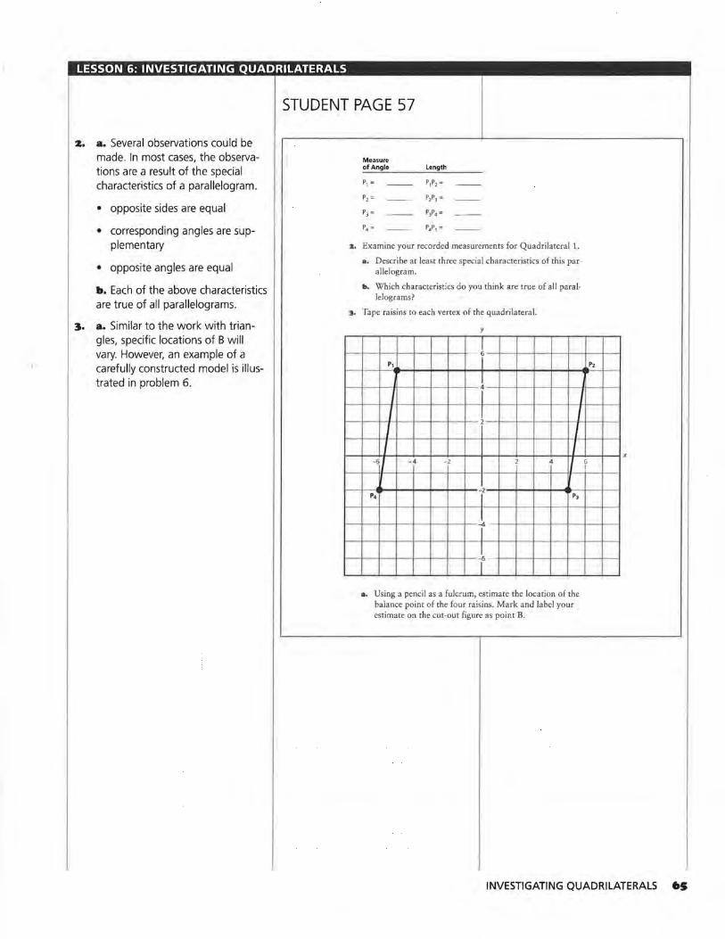
LESSON 6: INVESTIGATING QUADRILATERALS
z. a. Several observations could be made. In most cases, the observations are a result of the special characteristics of a parallelogram.
• opposite sides are equal
• corresponding angles are sup-plementary
• opposite angles are equal
b. Each of the above characteristics are true of all parallelograms.
:1. a. Similar to the work with triangles, specific locations of B will vary. However, an example of a carefully constructed model is illustrated in problem 6.
STUDENT PAGE 57
Measure of Angle Length
P, = P,P2 =
P, = P2PJ =
P3 = P,P, =
P4 = P.l1 =
z. Examine your recorded measurements for Quadrilateral 1.
a. Describe at least three special characteristics of this parallelogram.
b. Which characteristics do you think are true of all parallelograms?
~. Tape raisins to each vertex of the quadrilateral.
y
l~l--l--l--l'--1'--1---!-- 611 ---+--t--t---+--t--t--t--I P2 P1
1--+---<l--~t---+~-+--+~-1--- 1 ~+---+----<l----+--•~•1--+-~1 l--l-l---"'-1-1--1--l-l--l---t-i----+---+--<- H-' -t--1
1--<---<~--+--•~-+--+~+-- 2 ~+--1-~+---+----<~'----+~1 J
I I I I I
~ 1 - 4 -2
P4 P3 -,2-+-+--+--+--4.--il--t--1
1--1---<~--+--+~-+--~~+---~--<I--~·
l-t-->--t---+---+-t---~t--1---t---+-t---+---+-I
a. Using a pencil as a fulcrum, estimate the location of the balance point of the four raisins. Mark and label your estimate on the cut-out figure as point B.
INVESTIGATING QUADRILATERALS 65
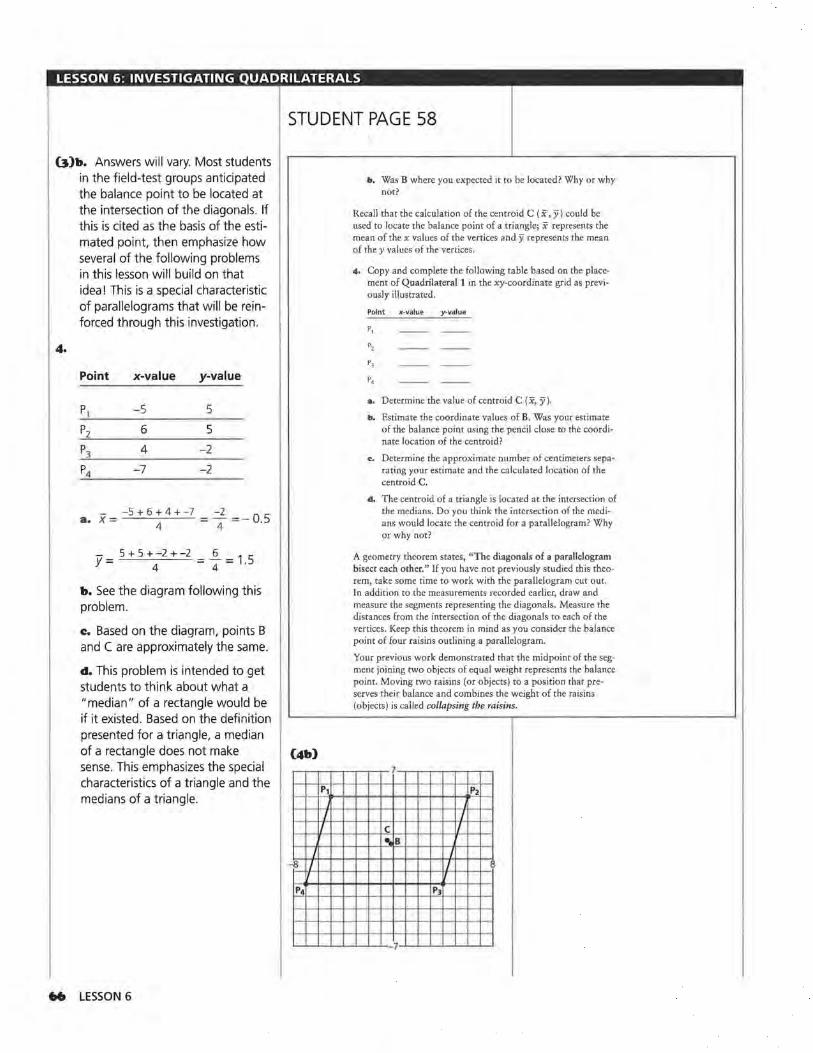
LESSON 6: INVESTIGATING QUADRILATERALS
U)b. Answers will vary. Most students in the field-test groups anticipated the balance point to be located at the intersection of the diagonals. If this is cited as the basis of the estimated point, then emphasize how several of the following problems in this lesson will build on that idea! This is a special characteristic of parallelograms that will be reinforced through this investigation.
Point x-value y-value
pl -5 5
P2 6 5
P3 4 -2
P4 -7 -2
- -5 + 6 + 4 + -7 -2 a. x =
4 = 4 = - 0.5
5 + 5 +-2 +-2 6 Y= 4 =4=1.5
b. See the diagram following this problem.
c. Based on the diagram, points B and C are approximately the same.
d. This problem is intended to get students to think about what a "median" of a rectangle would be if it existed . Based on the definition presented for a triangle, a median of a rectangle does not make sense. This emphasizes the special characteristics of a triangle and the medians of a triangle.
66 LESSON 6
STUDENT PAGE 58
(4b)
I I
I -8 I
b, Was B where you expected it to be located? Why or why not?
Recall that the calculation of the centroid C ( x, y) could be used to locate the balance point of a triangle; x represents the mean of the x values of the vertices and y represents the mean of they values of the vertices.
4. Copy and complete the following table based on the placement of Quadrilateral 1 in the xy-coordinate grid as previously illustrated.
Point K-value y-value
P,
r,
P,
a. Determine the value of centroid C (x, y).
b. Estimate the coordinate values of B. Was your estimate of the balance point using the pencil close to the coordinate location of the centroid?
'" Determine the approximate number of centimeters separating your estimate and the calculated location of the centroid C.
d, The centroid of a triangle is located at the intersection of the medians. Do you think the intersection of the medians would locate the centroid for a parallelogram? Why or why not?
A geometry theorem states, "The diagonals of a parallelogram bisect each other." If you have not previously studied this theorem, take some time to work with the parallelogram cut out. In addition to the measurements recorded earlier, draw and measure the segments representing the diagonals. Measure the distances from the intersection of the diagonals to each of the vertices. Keep this theorem in mind as you consider the balance point of four raisins outlining a parallelogram.
Your previous work demonstrated that the midpoint of the segment joining two objects of equal weight represents the balance point. Moving two raisins (or objects) to a position that preserves their balance and combines the weight of the raisins (objects) is called collapsing the raisins.
I c I
.. B I
I
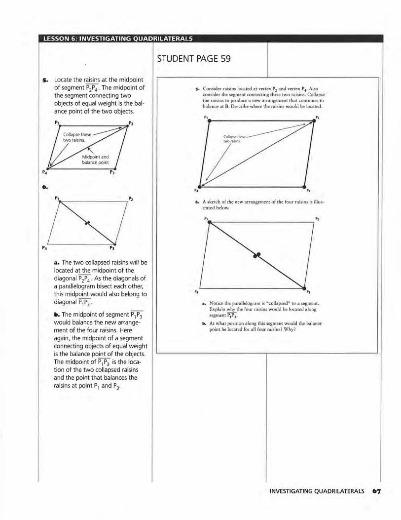
LESSON 6: INVESTIGATING QUADRILATERALS
s. Locate the raisins at the midpoint of segment P2P4 . The midpoint of the segment connecting two objects of equal weight is the balance point of the two objects.
P4
6.
P1
two raisins.
e P3
P1
a. The two collapsed raisins will be located at the midpoint of the diagonal P2P4 . As the diagonals of a parallelogram bisect each other, this midpoint would also belong to diagonal P1P3 .
b. The midpoint of segment P1P3 would balance the new arrangement of the four raisins. Here again, the midpoint of a segment connecting objects of equal weight is the balance point of the objects. The midpoint of P 1P3 is the location of the two collapsed raisins and the point that balances the raisins at point P1 and P3.
STUDENT PAGE 59
s. Consider raisins located at vertex P2 and vertex P4• Also consider the segment connecting these two raisins. Collapse the raisins to produce a new arrangement that continues to balance at B. Describe where the raisins would be located.
6. A sketch of the new arrangement of the four raisins is illustrated below.
a. Notice the parallelogram is "collapsed" to a segment. Explain why the four raisins would be located along segmentP~.
b. At what position along this segment would the balance point be located f~r all four raisins? Why?
INVESTIGATING QUADRILATERALS 67
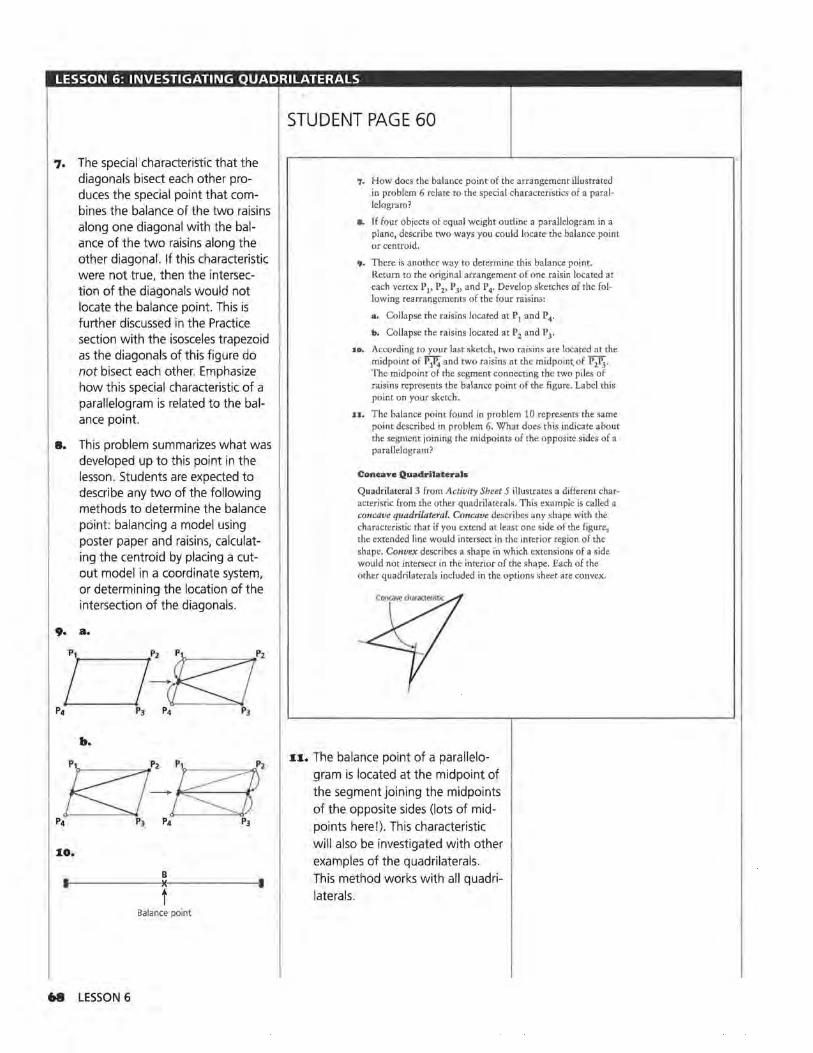
LESSON 6: INVESTIGATING QUADRILATERALS
7. The special characteristic that the diagonals bisect each other produces the special point that combines the balance of the two raisins along one diagonal with the balance of the two raisins along the other diagonal. If this characteristic were not true, then the intersection of the diagonals would not locate the balance point. This is further discussed in the Practice section with the isosceles trapezoid as the diagonals of this figure do not bisect each other. Emphasize how this special characteristic of a parallelogram is related to the balance point.
8. This problem summarizes what was developed up to this point in the lesson. Students are expected to describe any two of the following methods to determine the balance point: balancing a model using poster paper and raisins, calculating the centroid by placing a cutout model in a coordinate system, or determining the location of the intersection of the diagonals.
9. a.
b.
1.0.
I
68 LESSON 6
B )(
t Balance point
•
STUDENT PAGE 60
7. How does the balance point of the arrangement illustrated in problem 6 relate to the special characteristics of a parallelogram?
8. If four objects of equal weight outline a parallelogram in a plane, describe two ways you could locate the balance point or centroid.
9. There is another way to determine this balance point. Return to the original arrangement of one raisin located at each vertex P 1' P 2, P 3, and P 4• Develop sketches of the following rearrangements of the four raisins:
a. Collapse the raisins located at P 1 and P 4.
b. Collapse the raisins located at P z and P 3•
10. According to your last sketch, two raisins are located at the midpoint of PiP4 and two raisins at the midpoint.of P2P3•
The midpoint of the segment connecting the two piles of raisins represents the balance point of the figure. Label this point on your sketch.
:u. The balance point found in problem 10 represents the same point described in problem 6. What does this indicate about the segment joining the midpoints of the opposite sides of a parallelogram?
Concave Quadrilaterals
Quadrilateral 3 from Activity Sheet 5 illustrates a different characteristic from the other quadrilaterals. This example is called a concave quadrilateral. Concave describes any shape with the characteristic that if you extend at least one side of the figure, the extended line would intersect in the interior region of the shape. Convex describes a shape in which extensions of a side would not intersect in the interior of the shape. Each of the other quadrilaterals included in the options sheet are convex.
1.1.. The balance point of a parallelo
gram is located at the midpoint of
the segment joining the midpoints
of the opposite sides (lots of mid
points here!). This characteristic
will also be investigated with other
examples of the quadrilaterals.
This method works with all quadri
laterals.
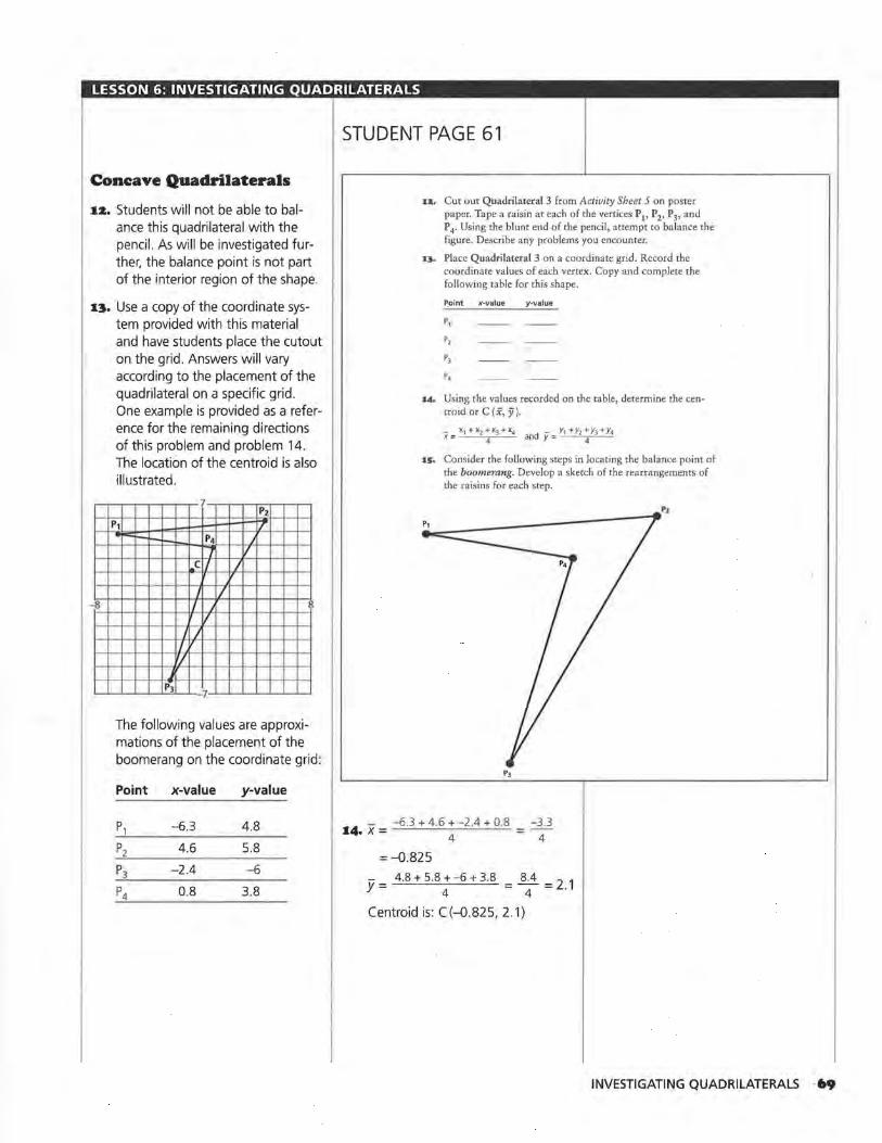
LESSON 6: INVESTIGATING QUADRILATERALS
Concave Quadrilaterals
1z. Students will not be able to balance this quadrilateral with the pencil. As will be investigated further, the balance point is not part of the interior region of the shape.
13. Use a copy of the coordinate system provided with this material and have students place the cutout on the grid. Answers will vary according to the placement of the quadrilateral on a specific grid. One example is provided as a reference for the remaining directions of this problem and problem 14. The location of the centroid is also illustrated.
7 P2
P1 I/ ·-r---- P4 J
J v c I I
If
' I I J
I I I
/ If
'I j
P3 7
The following values are approximations of the placement of the boomerang on the coordinate grid:
Point x-value y-value
P, -6.3 4.8
P2 4.6 5.8
P3 -2.4 -6
P4 0.8 3.8
STUDENT PAGE 61
u. Cut out Quadrilateral 3 from Activity Sheet 5 on poster paper. Tape a raisin at each of the vertices P1, P2, P3, and P 4• Using the blunt end of the pencil, attempt to balance the figure. Describe any problems you encounter.
u. Place Quadrilateral 3 on a coordinate grid. Record the coordinate values of each vertex. Copy. and complete the following table for this shape.
Ppint x-value y-value
P,
P2
P3
14. Using the values recorded on the table, determine the centroid or C (x, Y).
15. Consider the following steps in locating the balance point of the boomerang. Develop a sketch of the rearrangements of the raisins for each step.
14 - -6.3 + 4.6 + -2 .4 + 0.8 .x= 4 -3.3
4
=-0.825
y = 4.8 + 5 8 ;-6 + 3.8 = 8~4 = 2.1
Centroid is: C (-0.825, 2.1)
INVESTIGATING QUADRILATERALS ·69
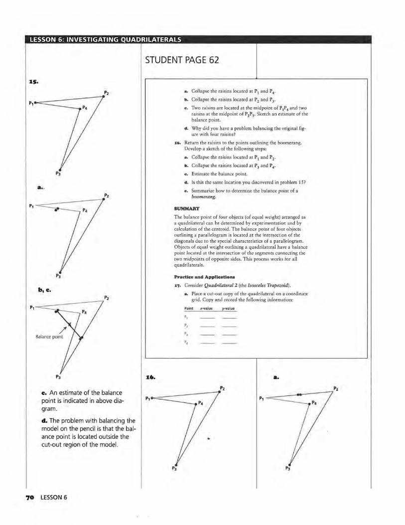
LESSON 6: INVESTIGATING QUADRILATERALS
a . .
b, c.
c. An estimate of the balance point is indicated in above diagram.
d, The problem with balancing the model on the pencil is that the balance point is located outside the cut-out region of the model.
70 LESSON 6
STUDENT PAGE 62
•••
a. Collapse the raisins located at P 1 and P 4.
b. Collapse the raisins located at P2 and Py
e. Two raisins are located at the midpoint of P1P4 and two raisins at the midpoint of P2P3• Sketch an estimate of the balance point.
d. Why did you have a problem balancing the original figure with four raisins?
:16. Return the raisins to the points outlining the boomerang. Develop a sketch of the following steps:
a. Collapse the raisins located at P1 and P2.
b. Collapse the raisins located at P 3 and P 4•
e. Estimate the balance point.
d. Is this the same location you discovered in problem 15?
e. Summarize how to determine the balance point of a boomerang.
SUMMARY
The balance point of four objects (of equal weight) arranged as a quadrilateral can be determined by experimentation and by calculation of the centroid. The balance point of four objects outlining a parallelogram is located at the intersection of the diagonals due to the special characteristics of a parallelogram. Objects of equal weight outlining a quadrilateral have a balance point located at the intersection of the segments connecting the two midpoints of opposite sides. This process works for all quadrilaterals.
Practice and Applications
:17. Consider Quadrilateral 2 (the Isosceles Trapezoid).
a. Place a cut-out copy of the quadrilateral on a coordinate grid. Copy and record the following information:
Point x-value y-value
P,
a.
..
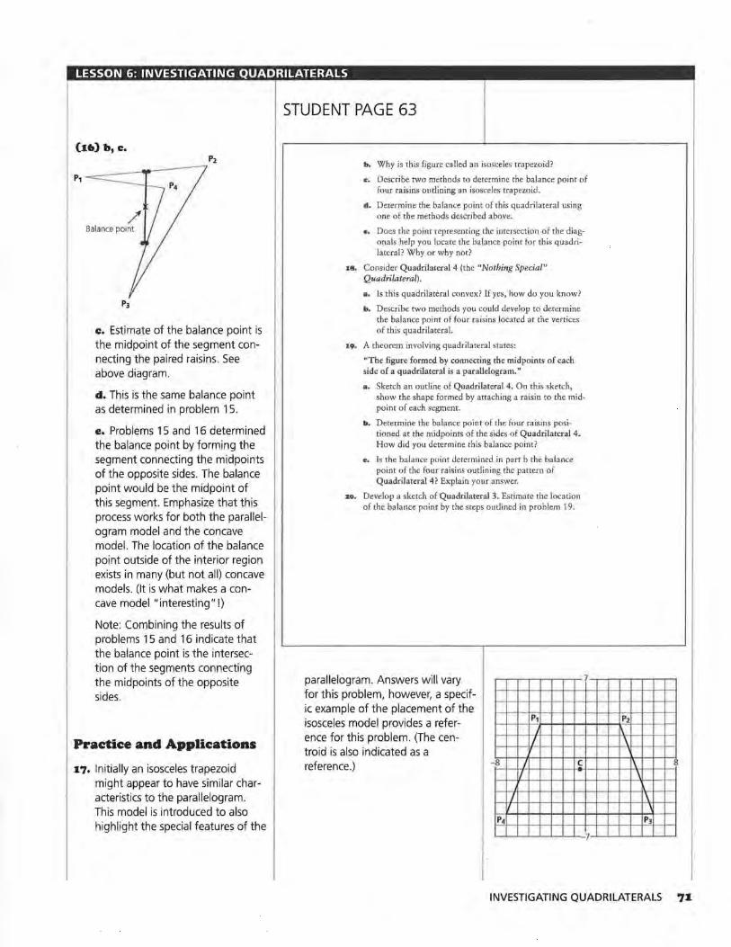
LESSON 6: INVESTIGATING QUADRILATERALS
(16) b, c.
c. Estimate of the balance point is the midpoint of the segment connecting the paired raisins. See above diagram.
d. This is the same balance point as determined in problem 15.
e. Problems 15 and 16 determined the balance point by forming the segment connecting the midpoints of the opposite sides. The balance point would be the midpoint of this segment. Emphasize that this process works for both the parallelogram model and the concave model. The location of the balance point outside of the interior region exists in many (but not all) concave models. (It is what makes a concave model "interesting"!)
Note: Combining the results of problems 15 and 16 indicate that the balance point is the intersection of the segments connecting the midpoints of the opposite sides.
Practice and Applications
17. Initially an isosceles trapezoid might appear to have similar characteristics to the parallelogram. This model is introduced to also highlight the special features of the
STUDENT PAGE 63
b, Why is this figure called an isosceles trapezoid?
c, Describe two methods to determine the balance point of four raisins outlining an isosceles trapezoid.
d, Determine the balance point of this quadrilateral using one of the methods described above.
e, Does the point representing the intersection of the diagonals help you locate the balance point for this quadrilateral? Why or why not?
18. Consider Quadrilateral 4 (the "Nothing Special" Quadrilateral).
a, Is this quadrilateral convex? If yes, how do you know?
b, Describe two methods you could develop tci determine the balance point of four raisins located at the vertices of this quadrilateral.
19. A theorem involving quadrilateral states:
"The figure formed by connecting the midpoints of each side of a quadrilateral is a parallelogram."
a. Sketch an outline of Quadrilateral 4. On this sketch, show the shape formed by attaching a raisin to the midpoint of each segment.
b, Determine the balance point of the four raisins positioned at the midpoints of the sides of Quadrilateral 4. How did you determine this balance point?
c. Is the balance point determined in part b the balance point of the four raisins outlining the pattern of Quadrilateral 4? Explain your answer.
zo. Develop a sketch of Quadrilateral 3. Estimate the location of the balance point by the steps outlined in problem 19.
parallelogram. Answers will vary 7
for this problem, however, a specif-ic example of the placement of the
P1 isosceles model provides a refer-ence for this problem. (The cen-
J
I troid is also indicated as a reference.) - 8 I c
I
I
P4
7
P2 \
\
\
' \
P3
INVESTIGATING QUADRILATERALS 7I
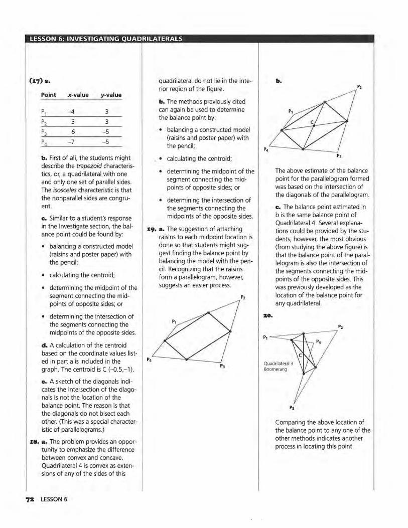
LESSON 6: INVESTIGATING QUADRILATERALS
(17) a.
Point x-value y-value
P1 -4 3
Pz 3 3
P3 6 -5
P4 -7 -5
b. First of all, the students might describe the trapezoid characteristics, or, a quadrilateral with one and only one set of parallel sides. The isosceles characteristic is that the nonparallel sides are congruent.
e. Similar to a student's response in the Investigate section, the balance point could be found by:
• balancing a constructed model (raisins and poster paper) with the pencil;
• calculating the centroid;
• determining the midpoint of the segment connecting the midpoints of opposite sides; or
• determining the intersection of the segments connecting the midpoints of the opposite sides.
d. A calculation of the centroid based on the coordinate values listed in part a is included in the graph. The centroid is C (-0.5,-1 ).
e. A sketch of the diagonals indicates the intersection of the diagonals is not the location of the balance point. The reason is that the diagonals do not bisect each other. (This was a special characteristic of parallelograms.)
18. a. The problem provides an opportunity to emphasize the difference between convex and concave. Quadrilateral 4 is convex as extensions of any of the sides of this
7Z LESSON 6
quadrilateral do not lie in the interior region of the figure.
b. The methods previously cited can again be used to determine the balance point by:
• balancing a constructed model (raisins and poster paper) with the pencil;
• calculating the centroid;
• determining the midpoint of the segment connecting the midpoints of opposite sides; or
• determining the intersection of the segments connecting the midpoints of the opposite sides.
19. a. The suggestion of attaching raisins to each midpoint location is done so that students might suggest finding the balance point by balancing the model with the pencil. Recognizing that the raisins form a parallelogram, however, suggests an easier process.
zo.
b.
The above estimate of the balance point for the parallelogram formed was based on the intersection of the diagonals of the parallelogram.
e. The balance point estimated in b is the same balance point of Quadrilateral 4. Several explanations could be provided by the students, however, the most obvious (from studying the above figure) is that the balance point of the parallelogram is also the intersection of the segments connecting the midpoints of the opposite sides. This was previously developed as the location of the balance point for any quadrilateral.
Quadrilateral 3 Boomerang
Comparing the above location of the balance point to any one of the other methods indicates another process in locating this point.
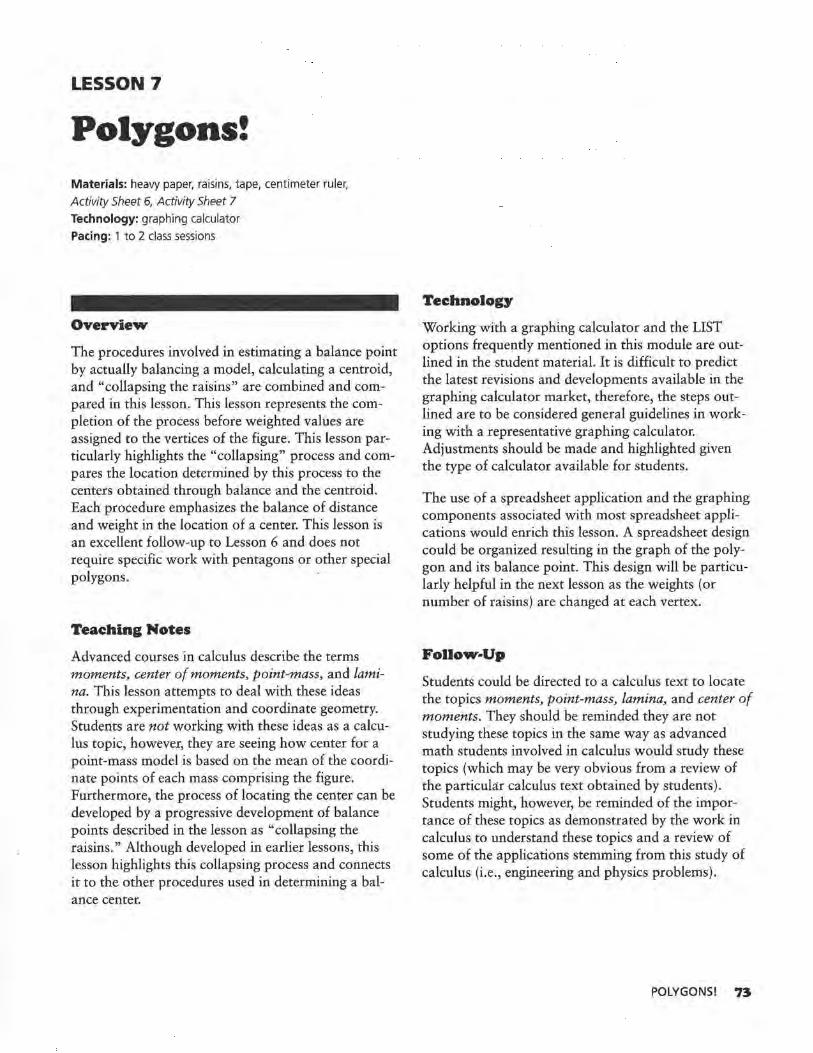
LESSON 7
Polygons! Materials: heavy paper, raisins, tape, centimeter ruler,
Activity Sheet 6, Activity Sheet 7 Technology: graphing calculator
Pacing: 1 to 2 class sessions
Overview
The procedures involved in estimating ~ balance p~int by actually balancing a model, calculatmg a centrmd, and "collapsing the raisins" are combined and compared in this lesson. This lesson represents the completion of the process before weighted values are assigned to the vertices of the figure. This lesson particularly highlights the "collapsing" process and compares the location determined by this process to ~he centers obtained through balance and the centrmd. Each procedure emphasizes the balance of distance and weight in the location of a center. This lesson is an excellent follow-up to Lesson 6 and does not require specific work with pentagons or other special polygons. -
Teaching Notes
Advanced courses in calculus describe the terms moments, center of moments, point-mass, and lamina. This lesson attempts to deal with these ideas through experimentation and coordinate geometry. Students are not working with these ideas as a calculus topic, however, they are seeing how center for a . point-mass model is based on the mean of the coordinate points of each mass comprising the figure. Furthermore, the process of locating the center can be developed by a progressive development of balance points described in the lesson as "collapsing the . raisins." Although developed in earlier lessons, this lesson highlights this collapsing process and connects it to the other procedures used in determining a balance center.
Technology
Working with a graphing calculator and the LIST options frequently mentioned in this module are ~utlined in the student material. It is difficult to predict the latest revisions and developments available in the graphing calculator market, therefore, the steps outlined are to be considered general guidelines in working with a representative graphing calculator. Adjustments should be made and highlighted given the type of calculator available for students.
The use of a spreadsheet application and the graphing components associated with most spreadsheet appl~cations would enrich this lesson. A spreadsheet design could be organized resulting in the graph of the polygon and its balance point. This design will be particularly helpful in the next lesson as the weights (or number of raisins) are changed at each vertex.
Follow-Up
Students could be directed to a calculus text to locate the topics moments, point-mass, lamina, and center of moments. They should be reminded they are not studying these topics in the same way as advanced math students involved in calculus would study these topics (which may be very obvious from a review of the particular calculus text obtained by students). Students might, however, be reminded of the importance of these topics as demonstrated by the work in calculus to understand these topics and a review of some of the applications stemming from this study of calculus (i.e., engineering and physics problems).
POLYGONS! 73
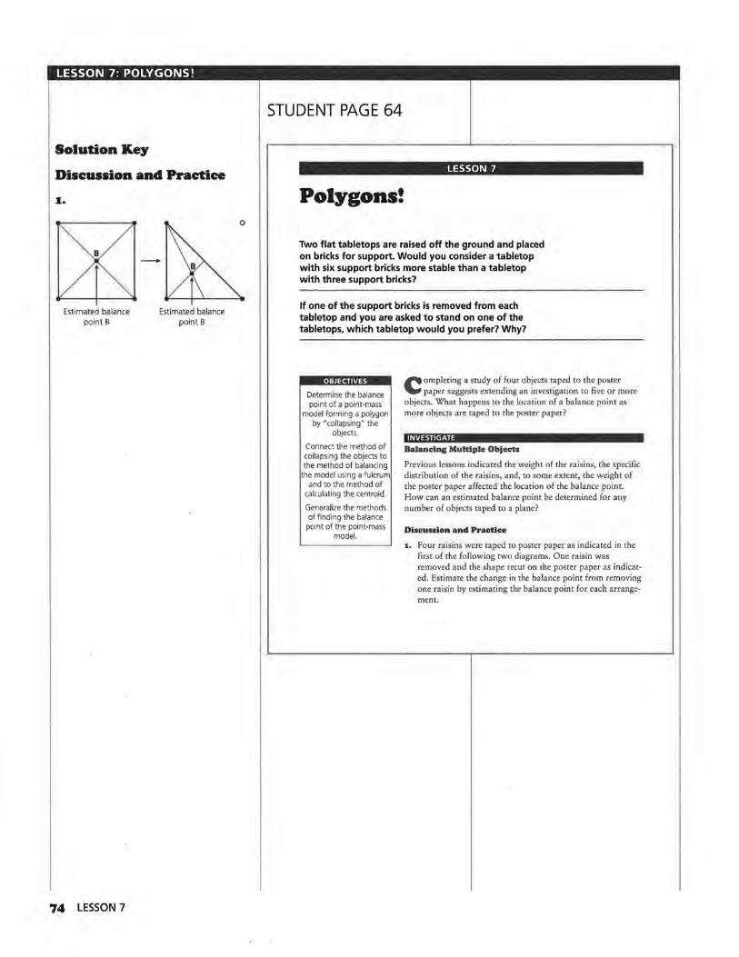
LESSON 7: POLYGONS!
Solution Key
Discussion and Practice
••
Estimated balance point B
74 LESSON 7
--Estimated balance
point B
0
STUDENT PAGE 64
LESSON 7
Polygons!
Two flat tabletops are raised off the ground and placed on bricks for support. Would you consider a tabletop with six support bricks more stable than a tabletop with three support bricks?
If one of the support bricks is removed from each tabletop and you are asked to stand on one of the tabletops, which tabletop would you prefer? Why?
, , Determine the balance point of a point-mass
model forming a polygon by "collapsing" the
objects.
Connect the method of collapsing the objects to the method of balancing the model using a fulcrum
and to the method of calculating the centroid.
Generalize the methods of finding the balance
point of the point-mass model.
C ompleting a study of four objects taped to the poster paper suggests extending an investigation to five or more
objects. What happens to the location of a balance point as more objects are taped to the poster paper?
INVESTIGATE
Balancing Multiple Objectll
Previous lessons indicated the weight of the raisins, the specific distribution of the raisins, and, to some extent, the weight of the poster paper affected the location of the balance point. How can an estimated balance point be determined for any number of objects taped to a plane?
DIRunlon and Practloe
:1. Four raisins were taped to poster paper as indicated in the first of the following two diagrams. One raisin was removed and the shape recut on the poster paper as indicated. Estimate the change in the balance point from removing one raisin by estimating the balance point for each arrangement.
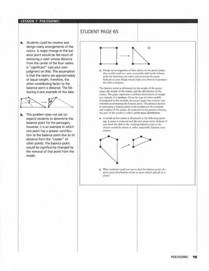
LESSON 7: POLYGONS!
:a. Students could be creative and design many arrangements of the raisins. A major change in the balance point would be the result of removing a raisin whose distance from the center of the four raisins is "significant" (use your own judgment on this). The assumption is that the raisins are approximately of equal weight, therefore, the other contributing factor to the balance point is distance. The following is one example of this idea:
3. This problem does not ask (or expect) students to determine the balance point for the pentagon, however, it is an example in which one point has a greater contribution to the balance point due to its distance from the "cluster" of other points. The balance point would be significantly changed by the removal of that point from the model.
STUDENT PAGE 65
:&. Design an arrangement of four raisins on the poster paper that would result in a more noticeable shift in the balance point by removing one raisin and recutting the paper. Indicate in your design which raisin you remove to produce the shift in balance.
The balance point is influenced by the weight of the poster paper, the weight of the raisins, and the distribution of the raisins. The paper represents a uniform distribution of weight (an example of a lamina). Given the type of raisin models investigated in this module, the poster paper has a minor contribution in estimating the balance point. The primary factors in estimating a balance point in the models are the locations and weights of the raisins. As indicated in the previous lessons,
· this part of the model is called a point-mass distribution.
:J., A model of five raisins is illustrated in the following drawing. A raisin is removed and the new shape recut. Indicate if you think the shift in the resulting balance point of the objects would be minor or rather noticeable. Explain your answer.
4, What methods could you use to find the balance point of a point-mass distribution of five or more objects placed on a plane?
POLYGONS! 75
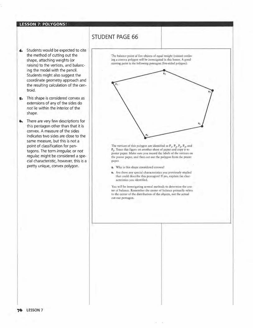
LESSON 7: POLYGONS!
4. Students would be expected to cite the method of cutting out the shape, attaching weights (or raisins) to the vertices, and balancing the model with the pencil. Students might also suggest the coordinate geometry approach and the resulting calculation of the centroid .
5. This shape is considered convex as extensions of any of the sides do not lie within the interior of the shape.
6. There are very few descriptions for this pentagon other than that it is convex. A measure of the sides indicates two sides are close to the same measure, but this is not a point of classification for pentagons. The term irregular, or not regular, might be considered a special characteristic, however, this is a pretty unique, convex polygon.
7• LESSON 7
STUDENT PAGE 66
The balance point of five objects of equal weight (raisins) outlining a convex polygon will be investigated in this lesson. A good starting point is the following pentagon (five-sided polygon):
The vertices of this polygon are identified as P 1, P 2, P 3, P 4, and P5. Trace this figure on another sheet of paper and copy it to poster paper. Make sure you record the labels of the vertices on the poster paper, and then cut out the polygon from the poster paper.
5. Why is this shape considered convex?
•· Are there any special characteristics you previously studied that could describe this pentagon? If yes, explain the characteristics you identified.
You will be investigating several methods to determine the center of balance. Remember the center of balance primarily refers to the center of the distribution of the objects, not the actual cut-out pentagon.
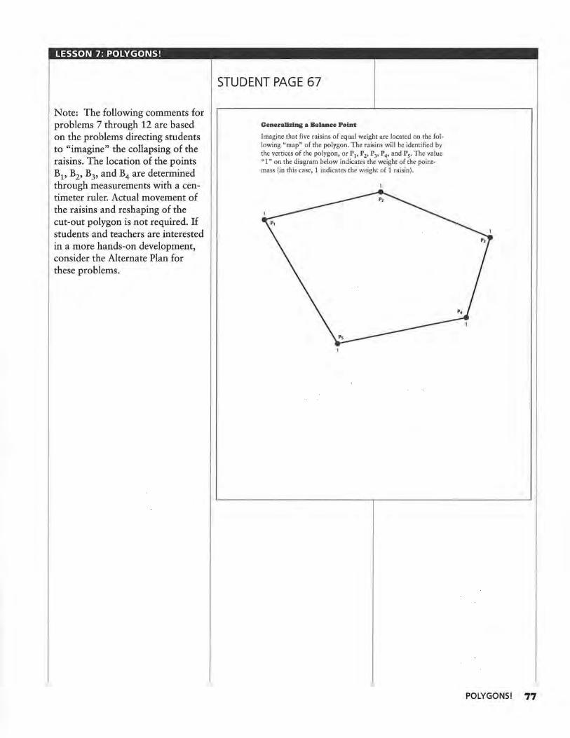
LESSON 7: POLYGONS!
Note: The following comments for problems 7 through 12 are based on the problems directing students to "imagine" the collapsing of the raisins. The location of the points B1, B2, B3, and B4 are determined through measurements with a centimeter ruler. Actual movement of the raisins and reshaping of the cut-out polygon is not required. If students and teachers are interested in a more hands-on development, consider the Alternate Plan for these problems.
STUDENT PAGE 67
Generalizing a Balance Point
Imagine that five raisins of equal weight are located on the following "map" of the polygon. The raisins will be identified by the vertices of the polygon, or P1, P2, P3, P4, and P5• The value "1" on the diagram below indicates the weight of the pointmass (in this case, 1 indicates the weight of 1 raisin).
POLYGONS! 77
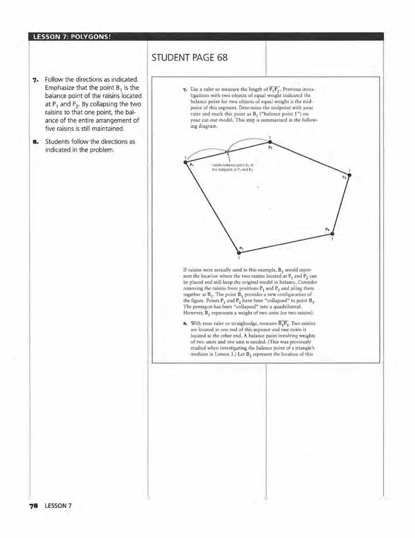
LESSON 7: POLYGONS!
7. Follow the directions as indicated. Emphasize that the point B1 is the balance point of the raisins located at P1 and P2. By collapsing the two raisins to that one point, the balance of the entire arrangement of five raisins is still maintained.
8. Students follow the directions as indicated in the problem.
78 LESSON 7
STUDENT PAGE 68
7, Use a ruler to measure the length of P 1P2 . Previous investigations with two objects of equal weight indicated the balance point for two objects of equal weight is the midpoint of this segment. Determine the midpoint with your ruler and mark this point as B1 ("balance point 1 ")on your cut-out model. This step is summarized in the foJJowing diagram.
Locate balance point 81 at the midpoint of P1 and P2
If raisins were actually used in this example, B 1 would represent the location where the two raisins located at P1 and P2 can be placed and still keep the original model in balance. Consider removing the raisins from positions P1 and P2 and piling them together at B1. The point B1 provides a new configuration of the figure . Points P1 and P2 have been "collapsed" to point B1.
The pentagon has been "collapsed" into a quadrilateral. However, B1 represents a weight of two units (or two raisins).
8. With your ruler or straightedge, measure B1P3. Two raisins are located at one end of this segment and one raisin is located at the other end. A balance point involving weights of two units and one umt is needed. (This was previously studied when investigating the balance point of a triangle's medians in Lesson 5.) Let B2 represent the location of this
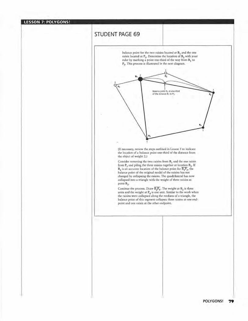
LESSON 7: POLYGONS!
STUDENT PAGE 69
balance point for the two raisins located at B1 and the one raisin located at P 3• Determine the location of B2 with your ruler by marking a point one-third of the way from B1 to P3. This process is illustrated in the next diagram.
e, 2
r Balance point 82 at one-third of the distance 81 to P3~
(If necessary, review the steps outlined in Lesson 5 to indicate the location of a balance point one-third of the distance from the object of weight 2.)
Consider removing the two raisins from B1 and the one raisin from P3 and piling the three raisins together at location B2• If B2 is an accurate location of the balance point for B1P3, the balance point of the original model of the raisins has not changed by collapsing the raisins. The quadrilateral has now collapsed into a triangle with the weight of three raisins at point B2.
Continue the process. Draw B2P 4 • The weight at B2 is three units and the weight at P 4 is one unit. Similar to the work when the raisins were collapsed along the medians of a triangle, the balance point of this segment collapses three raisins at one endpoint and one raisin at the other endpoint.
POLYGONS! 79
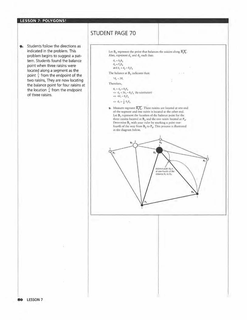
LESSON 7: POLYGONS!
9. Students follow the directions as indicated in the problem. This problem begins to suggest a pattern. Students found the balance point when three raisins were located along a segment as the point + from the endpoint of the two raisins, They are now locating the balance point for four raisins at the location ± from the endpoint of three raisins.
80 LESSON 7
STUDENT PAGE 70
Let B3 represent the point that balances the raisins along B2P4 •
Also, represent d1 and d2 such that:
d, = 0203
d2 = P4 B3
and d1 + d2 = B2P4
The balance at B3 indicates that:
1d, = 3d,
Therefore,
d1 +d2 =B2P4
=> d1 + 3d 1 = B2P4 (By substitution) => 4d 1 = B2P4
=> d1 = + B2P4
9, Measure segment B2P4 . Three raisins are located at one end of the segment and one raisin is located at the other end. Let B3 represent the location of the balance point for the three raisins located at B2 and the one raisin located at P4.
Determine B3 with your ruler by marking a point onefourth of the way from B2 to P 4. This process is illustrated in the diagram below.
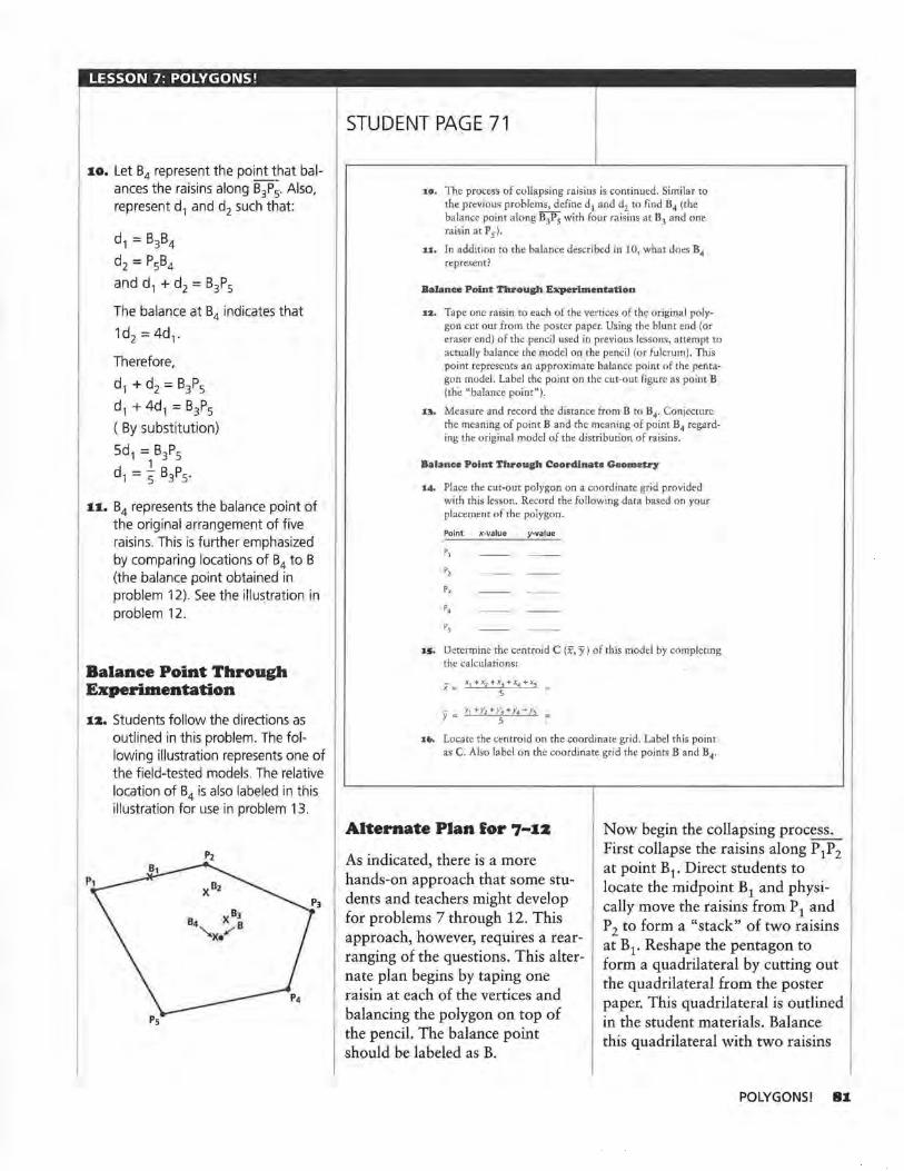
LESSON 7: POLYGONS!
10. Let B4 represent the point that balances the raisins along B3 P~. Also, represent d1 and d2 such that:
d1 = B3B4
d2 = P5B4 and d1 + d2 = B3P5
The balance at B4 indicates that
1d2=4d,.
Therefore,
d1 + d2 = B3P5
d1 + 4d1 = B3P5
( By substitution)
5d1 = Bls 1
d, = s B3P5.
11. B4 represents the balance point of the original arrangement of five raisins. This is further emphasized by comparing locations of B4 to B (the balance point obtained in problem 12). See the illustration in problem 12.
Balance Point Through Experimentation
12. Students follow the directions as outlined in this problem. The following illustration represents one of the field-tested models. The relative location of B4 is also labeled in this illustration for use in problem 13.
STUDENT PA~E 71
J:O. The process of collapsing raisins is continued. Similar to the previous problems, define d1 and d2 to find B4 (the balance point along B3P5 with four raisins at B3 and one raisin at P5 ).
u. In addition to the balance described in 10, what does B4 represent?
Balance Point Through EJKperimentation
:az. Tape one raisin to each of the vertices of the original polygon cut out from the poster paper. Using the blunt end (or eraser end) of the pencil used in previous lessons, attempt to actually balance the model on the pencil (or fulcrum). This point represents an approximate balance point of the pentagon model. Label the point on the cut-out figure as point B (the "balance point").
1:t. Measure and record the distance from B to B4. Conjecture the meaning of point B and the meaning of point B4 regarding the original model of the distribution of raisins.
Balance Point Through Coordinate Geometry
14. Place the cut-out polygon on a coordinate grid provided with this lesson. Record the following data based on your placement of the polygon.
Point x-value y-value
P,
15. Determine the centroid C (x, y) of this model by completing the calculations:
; = X1 + x2 + X3 + X4 + X5
5
y -= Y1 +Yi + Y~ + Y4 + Ys ~
1c.. Locate the centroid on the coordinate grid. Label this point as C. Also label on the coordinate grid the points Band B4•
Alternate Plan for 7-12
As indicated, there is a more hands-on approach that some students and teachers might develop for problems 7 through 12. This approach, however, requires a rearranging of the questions. This alternate plan begins by taping one raisin at each of the vertices and balancing the polygon on top of the pencil. The balance point should be labeled as B.
Now begin the collapsing process. First collapse the raisins along P 1P2 at point B1. Direct students to locate the midpoint B1 and physically move the raisins from P 1 and P2 to form a "stack" of two raisins at B1. Reshape the pentagon to form a quadrilateral by cutting out the quadrilateral from the poster paper. This quadrilateral is outlined in the student materials. Balance this quadrilateral with two raisins
POLYGONS! 8X
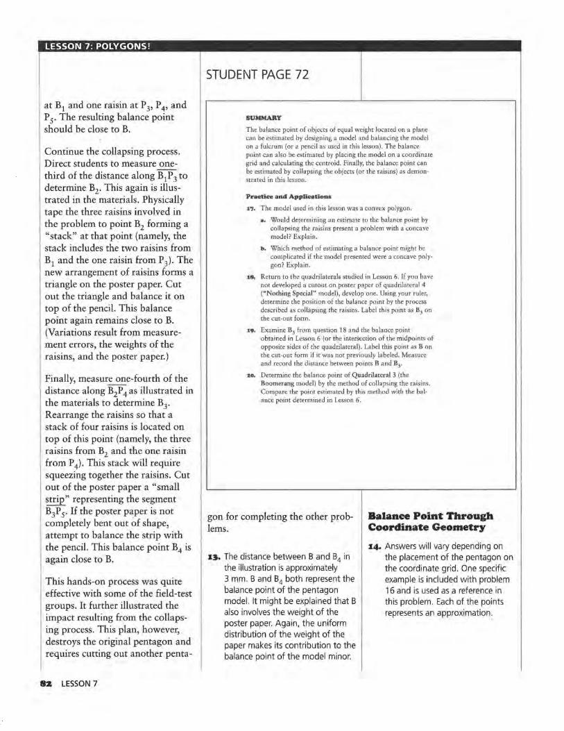
LESSON 7: POLYGONS!
at B1 and one raisin at P 3, P 4 , and P 5• The resulting balance point should be close to B.
Continue the collapsing process. Direct students to measure onethird of the distance along B1P3 to determine B2. This again is illustrated in the materials. Physically tape the three raisins involved in the problem to point B2 forming a "stack" at that point (namely, the stack includes the two raisins from B1 and the one raisin from P3 ). The new arrangement of raisins forms a triangle on the poster paper. Cut out the triangle and balance it on top of the pencil. This balance point again remains close to B. (Variations result from measurement errors, the weights of the raisins, and the poster paper.)
Finally, measure one-fourth of the distance along B2P 4 as illustrated in the materials to determine By Rearrange the raisins so that a stack of four raisins is located on top of this point (namely, the three raisins from B2 and the one raisin from P 4). This stack will require squeezing together the raisins. Cut out of the poster paper a "small strip" representing the segment B3P y If the poster paper is not completely bent out of shape, attempt to balance the strip with the pencil. This balance point B4 is again close to B.
This hands-on process was quite effective with some of the field-test groups. It further illustrated the impact resulting from the collapsing process. This plan, however, destroys the original pentagon and requires cutting out another penta-
8Z LESSON 7
STUDENT PAGE 72
SUMMARY
The balance point of objects of equal weight located on a plane can be estimated by designing a model and balancing the model on a fulcrum (or a pencil as used in this lesson). The balance point can also be estimated by placing the model on a coordinate grid and calculating the centroid. Finally, the balance point can be estimated by collapsing the objects (or the raisins) as demonstrated in this lesson.
Practice and Applications
n. The model used in this lesson was a convex polygon.
a. Would determining an estimate to the balance point by collapsing the raisins present a problem with a concave model? Explain.
b. Which method of estimating a balance point might be complicated if the model presented were a concave polygon? Explain.
18, Return to the quadrilaterals studied in Lesson 6. If you have not developed a cutout on poster paper of quadrilateral 4 ("Nothing Special" model), develop one. Using your ruler, determine the position of the balance point by the process described as collapsing the raisins. Label this point as B3 on the cut-out form .
19. Examine B3 from question 18 and the balance point obtained in Lesson 6 (or the intersection of the midpoints of opposite sides of the quadrilateral) . Label this point as Bon the cut-out form if it was not previously labeled. Measure and record the distance between points B and B3.
,.o. Determine the balance point of Quadrilateral 3 (the Boomerang model) by the method of collapsing the raisins. Compare the point estimated by this method with the balance point determined in Lesson 6.
gon for completing the other problems.
1::1. The distance between B and 84 in the illustration is approximately 3 mm. B and 84 both represent the balance point of the pentagon model. It might be explained that B also involves the weight of the poster paper. Again, the uniform distribution of the weight of the paper makes its contribution to the balance point of the model minor.
Balance Point Through Coordinate Geometry
1:4. Answers will vary depending on the placement of the pentagon on the coordinate grid. One specific example is included with problem 16 and is used as a reference in this problem. Each of the points represents an approximation:
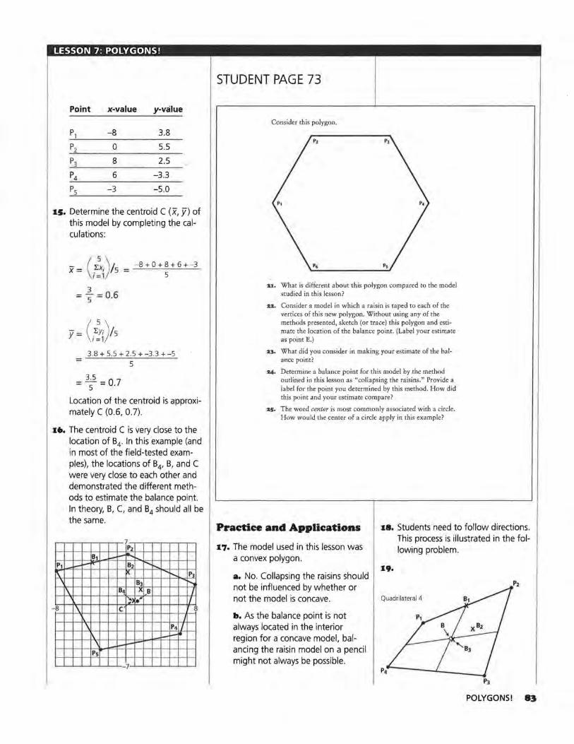
LESSON 7: POLYGONS!
Point x-value y-value
P, -8 3.8
Pz 0 5.5
P3 8 2.5
P4 6 -3.3
Ps -3 -5.0
15. Determine the centroid C (x, fl of this model by completing the calculations:
x= (/x;)/5 = I =1
3 = - = 06 5 .
y = (ir;)/5 1=1
-8 + 0 + 8 + 6 + -3 5
= 3.8 + 5.5 + 2.5 + -3.3 + -5
5
=3~5=0.7
Location of the centroid is approximately C (0.6, 0.7).
16. The centroid C is very close to the location of 84 . In this example (and in most of the field-tested examples), the locations of 84, 8, and C were very close to each other and demonstrated the different methods to estimate the balance point. In theory, 8, C, and 84 should all be the same.
7 P2
81 --P1 ........ -"" 82 I" ......
I\ x. ~"'-- P•
' 83 r---, I\ 114 l\ 8 I
'!') •" I I\ C'
J
\ P~ I '\ i--' --_ .......
Ps
7
STUDENT PAGE 73
Consider this polygon.
n. What is different about this polygon compared to the model studied in this lesson?
zz. Consider a model in which a raisin is taped to each of the vertices of this new polygon. Without using any of the methods presented, sketch (or trace) this polygon and estimate the location of the balance point. (Label your estimate as point E.)
zJ, What did you consider in making your estimate of the balance point?
Z4· Determine a balance point for this model by the method outlined in this lesson as "collapsing the raisins." Provide a label for the point you determined by this method. How did this point and your estimate compare?
zs, The word center is most commonly associated with a circle. How would the center of a circle apply in this example?
Practice and Applications 18. Students need to follow directions.
17. The model used in this lesson was a convex polygon.
a. No. Collapsing the raisins should not be influenced by whether or
19.
This process is illustrated in the following problem.
not the model is concave. Quadrilateral 4
h. As the balance point is not always located in the interior region for a concave model, balancing the raisin model on a pencil might not always be possible.
POLYGONS! 83
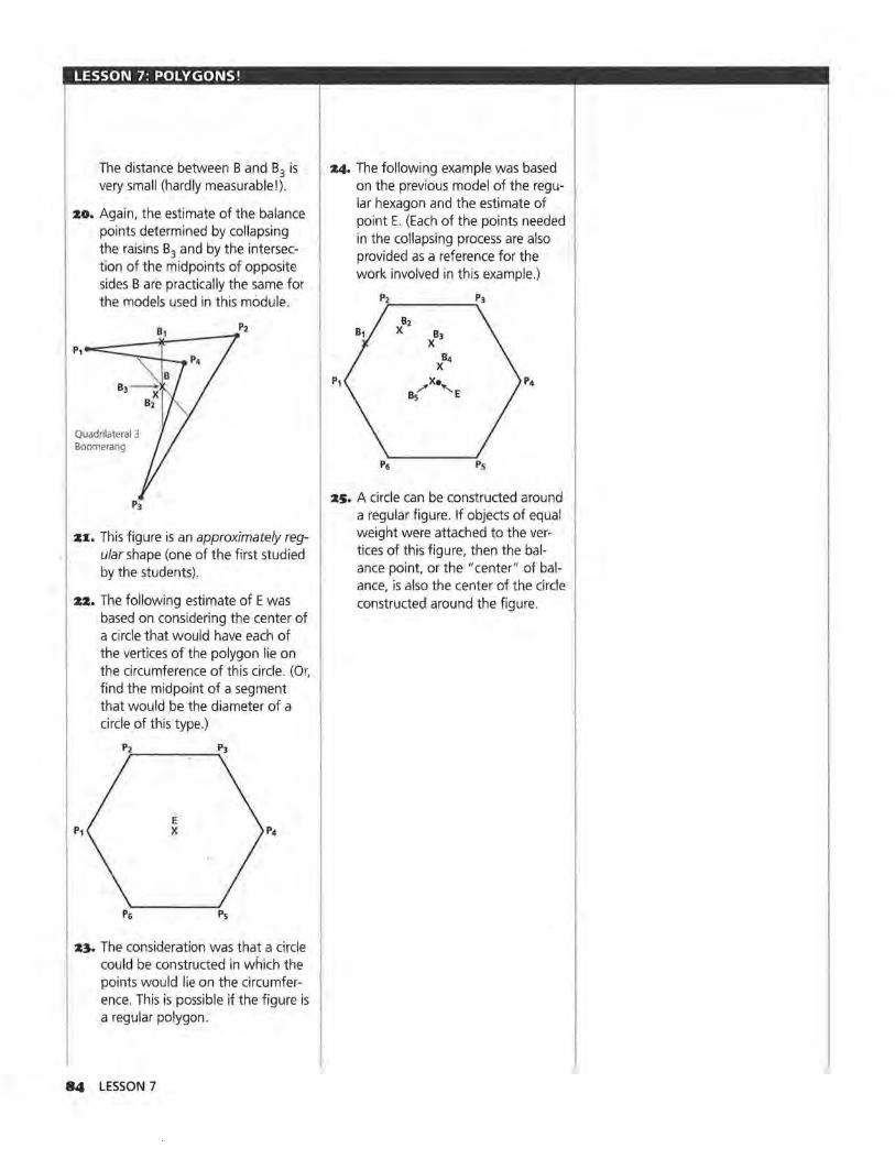
LESSON 7: POLYGONS!
The distance between B and B3 is very small (hardly measurable!).
zo. Again, the estimate of the balance points determined by collapsing the raisins 83 and by the intersection of the midpoints of opposite sides B are practically the same for the models used in this module.
Quadrilateral 3 Boomerang
:&1. This figure is an approximately regular shape (one of the first studied by the students).
:&:&. The following estimate of E was based on considering the center of a circle that would have each of the vertices of the polygon lie on the circumference of this circle. (Or, find the midpoint of a segment that would be the diameter of a circle of this type.)
P,_2 ____ _.,.Pl
E x
Ps
:&~. The consideration was that a circle could be constructed in which the points would lie on the circumference. This is possible if the figure is a regular polygon .
84 LESSON 7
z4. The following example was based on the previous model of the regular hexagon and the estimate of point E. (Each of the points needed in the collapsing process are also provided as a reference for the work involved in this example.)
82 x 83 x
84 x P1 ,..,,x., P4
85 E
:as. A circle can be constructed around a regular figure. If objects of equal weight were attached to the vertices of this figure, then the balance point, or the "center" of balance, is also the center of the circle constructed around the figure.
LESSON 8
Weighted Means Revisited Materials: heavy paper, raisins, tape, centimeter ruler,
Activity Sheet 6, Activity Sheet 7, Unit Ill Quiz
Technology: graphing calculator
Pacing: 1 to 2 class sessions
Overview
Taping more than one raisin to each of the vertices of the pentagon model will shift the balance point previously determined in Lesson 7. The weighted vertices shift the center in the direction of the heavier pile of raisins. This location can again be estimated by calculating the centroid as directed in the text. The means involved in these calculations, however, require the weighted values be included in the calculations. The specifics of this extension are tied back to the weighted means obtained in Lesson 4. This lesson essentially demonstrates how this is expanded to a two-dimen-sional model. . .
Teaching Notes
The raisins taped to the vertices of the pentagon again produce a workable model in estimating the balance point of this figure. The point obtained from balancing the figure on a pencil and the point derived from the weighted means will not be as close as in the previous models. Many factors could be used to explain this (i.e., the varying weights of the raisins or the "spread" of the weights obtained from piling raisins on top of each other at the vertices). Essentially, this lesson completes the models involved in taping raisins as an estimate of locating the balance point. The process was developed as a way to highlight the balance of weight and distance in the problems described to the students.
Technology
Working with a graphing calculator and the LIST options is required in this lesson. The data needed to determine the center are organized in the student material for easy entry into a graphing calculator (specifically the TI-82 or TI-83 models).
As indicated in Lesson 7, the use of a spreadsheet application and the graphing components associated with most spreadsheet applications would enrich this lesson. A spreadsheet design could be organized resulting in the graph of the polygon and its balance point. Varying the raisin count on the spreadsheet and observing the resulting change in the balance point is a powerful way to complete the discussion of this type of center! .
WEIGHTED MEANS REVISITED 85
LESSON 8: WEIGHTED MEANS REVISITED
86 LESSON 8
STUDENT PAGE 74
LESSON 8
Weighted Means Revisited
Examine again the pentagon cut out of the poster paper in Lesson 7. How do you think the balance point of the pentagon model would change if the weight placed at vertex P1 was doubled?
Tape a second raisin to the model at P1 and balance it with the pencil. Did it change as you predicted?
A more precise location of this balance point is needed to determine the effect of the increased weight at P1•
What makes the calculation of a centroid more difficult if unequal weights are located at the vertices?
Determine the center of balance by calculating
the weighted means of the x- and y-coordinates
of objects distributed on a plane
Interpret the balance point by weights and locations
Using a pencil to balance a pentagon with a raisin taped at each vertex was a relatively good model to estimate a cen
ter of balance of five weights. To what extent does changing the weight of the raisins or their locations on a plane alter the location of the balance point? What if the weight taped at one vertex of the pentagon model was doubled by taping a second raisin over the one already located there? How would this additional weight change the balance point? Similarly, what if a weight were completely removed from a vertex? How would this change the balance point? An earlier lesson taped several raisins at a specific location on a ruler. Increasing the weight at this point altered the location of the fulcrum to balance the new arrangement of raisins. Several questions were investigated related to that balance point. This lesson examines similar 4uesliuns using a two-dimensional model.
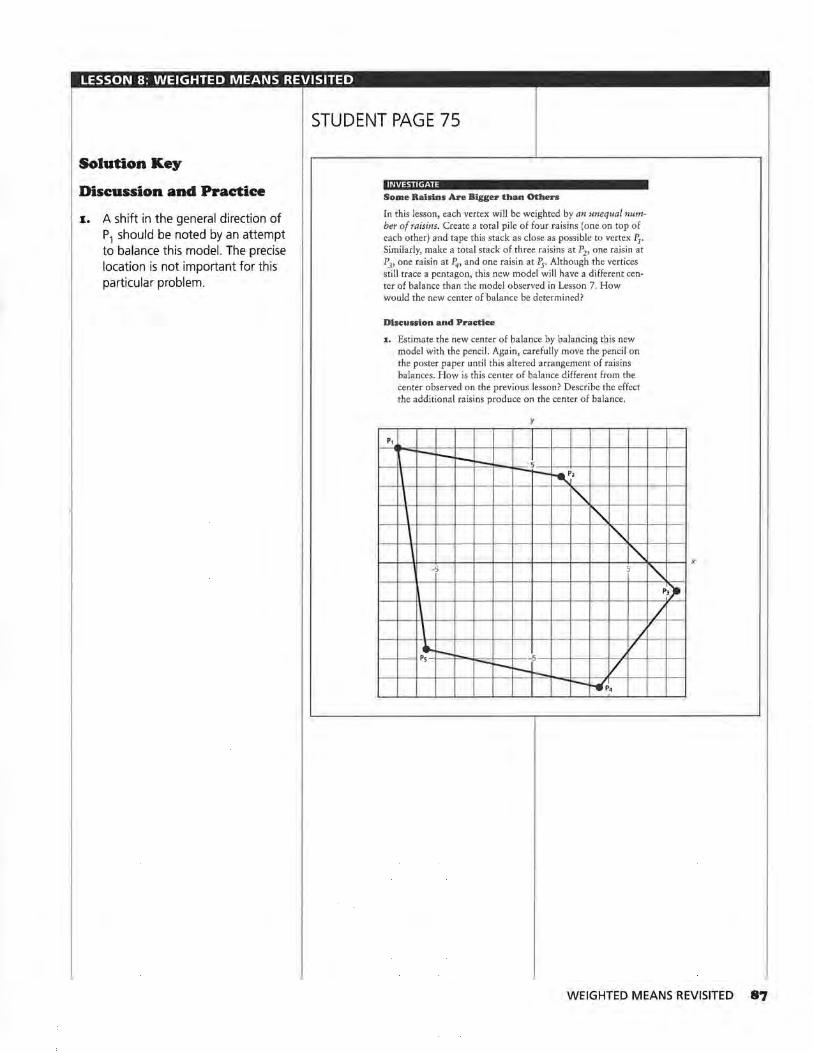
LESSON 8: WEIGHTED MEANS REVISITED
STUDENT PAGE 75
Solution Key
Discussion and Practice
i:. A shift in the general direction of P1 should be noted by an attempt to balance this model. The precise location is not important for this particular problem.
INVESTIGATE
Some Raisins Are Bigger than Others
In this lesson, each vertex will be weighted by an unequal number of raisins. Create a total pile of four raisins (one on top of each other) and tape this stack as close as possible to vertex IJ. Similarly, make a total stack of three raisins at P2 , one raisin at P3, one raisin at f4, and one raisin at P5. Although the vertices still trace a pentagon, this new model will have a different center of balance than the model observed in Lesson 7. How would the new center of balance be determined?
Discussion and Practice
1. Estimate the new center of balance by balancing this new model with the pencil. Again, carefully move the pencil on the poster paper until this altered arrangement of raisins balances. How is this center of balance different from the center observed on the previous lesson? Describe the effect the additional raisins produce on the center of balance.
y
P1
r--r-- I r---,_ 5 ~ -~' 1- \
" \ " \ " \ " -5 5
/ ... / - ~ - - Ps -s ~ -f--L_ /
r--r-"P,
" p~ / ,
WEIGHTED MEANS REVISITED 87
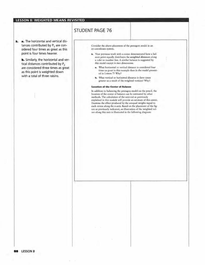
LESSON 8: WEIGHTED MEANS REVISITED
STUDENT PAGE 76
2. a. The horizontal and vertical distances contributed by P1 are considered four times as great as this point is four times heavier.
b. Similarly, the horizontal and vertical distances contributed by P2 are considered three times as great as this point is weighted down with a total of three raisins.
88 LESSON 8
Consider the above placement of the pentagon model in an xy-coordinate system.
z. Your previous work with a center demonstrated how a balance point equally distributes the weighted distances along a ruler or number line. A similar balance is suggested by this model except in two dimensions.
a. What horizontal or vertical distance is considered four times as great in this example than in the model presented in Lesson 7? Why?
b. What vertical or horizontal distance is three times greater as a result of the weighted vertices? Why?
Location of the Center of Balance
In addition to balancing the pentagon model on the pencil, the location of the center of balance can be estimated by other methods. The calculation of the centroid as previously explained in this module will provide an estimate of this center. Examine the effect produced by the unequal weights taped to each vertex along the x-axis. Based on the placement of the figure as previously indicated, an illustration of the weighted values along this axis is illustrated in the following diagram:
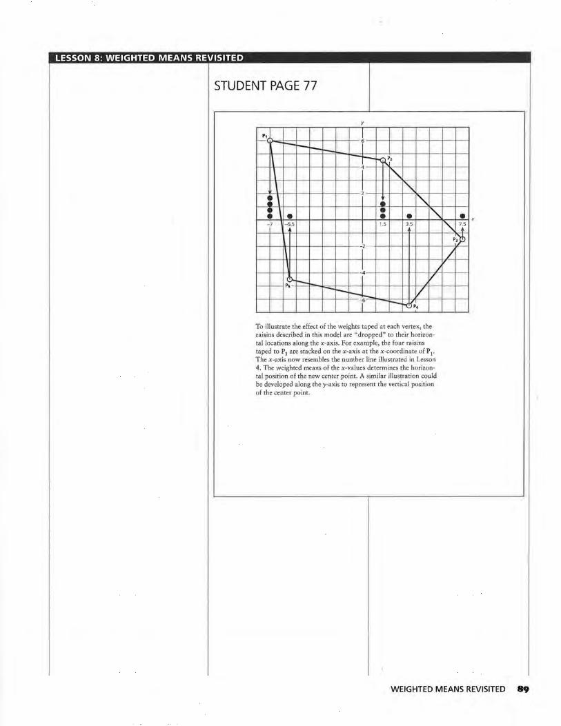
LESSON 8: WEIGHTED MEANS REVISITED
STUDENT PAGE 77
y
P1 I 6 r--r-r-- I ~
"'!('' I 4
"\... \ I \ "\... :• \
2
"' • ~. \ • "' • • • - 7 -5.5 1.5 3.5
- 2
I I /
-4 / I).. I Ps - ,
~ --L / 1 r--K!fP,
To illustrate the effect of the weights taped at each vertex, the raisins described in this model are "dropped" to their horizontal locations along the x-axis. For example, the four raisins taped to P1 are stacked on the x-axis at the x-coordinate of P1.
The x-axis now resembles the number line illustrated in Lesson 4. The weighted means of the x-values determines the horizontal position of the new center point. A similar illustration could be developed along the y-axis to represent the vertical position of the center point.
• ."\. 7.5 .. p~
/
WEIGHTED MEANS REVISITED 89
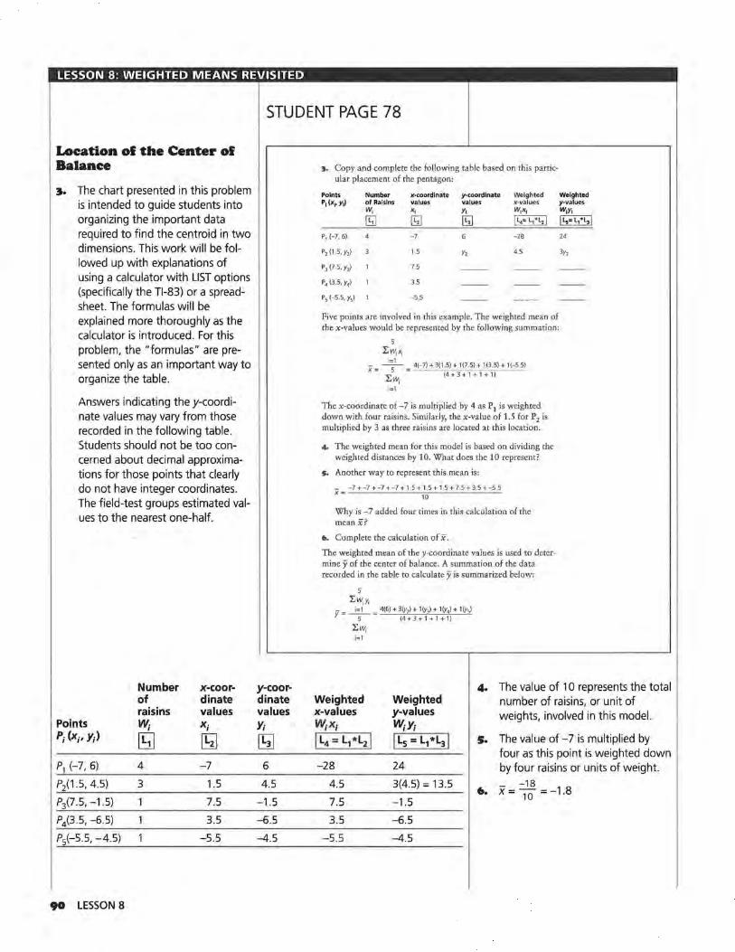
LESSON 8: WEIGHTED MEANS REVISITED
STUDENT PAGE 78
Location of the Center of Balance
:1. The chart presented in this problem is intended to guide students into organizing the important data required to find the centroid in two dimensions. This work will be followed up with explanations of using a calculator with LIST options (specifically the Tl-83) or a spreadsheet. The formulas will be explained more thoroughly as the calculator is introduced. For this problem, the "formulas" are presented only as an important way to organize the table.
Answers indicating the y-coordinate values may vary from those recorded in the following table. Students should not be too concerned about decimal approximations for those points that clearly do not have integer coordinates. The field-test groups estimated values to the nearest one-half.
Number x-coor-of dinate raisins values
Points W; X; P; (x;, Y;) [SJ ~ P1 (-7, 6) 4 -7
P2(1.5, 4.5) 3 1.5
Pp.5, -1.5) 7.5
P4(3.5, -6.5) 3.5
P5(-5.5, -4.5) -5.5
90 LESSON 8
y-coor-dinate values Y; [5J
6
4.5
-1.5
-6.5
-4.5
~. Copy and complete the following table based on this particular placement of the pentagon:
Points Number x-coordinate y-coordlnate Weighted P1(x1,y1) of Raisins values values x-values
w, x, y, W1X1
[SJ [Q [Q I L4= L, •i., I P1 (-7, 6) 4 -7 -28
P2 (1 5, y2) 1 5 Y2 4.5
P3 (7 5, y3) 75
P4 (3 5, y4) 3.5
P5 (-5 .5,y5) 1 -5 5
Five points are involved in this example. The weighted mean of the x-values would be represented by the following summation:
5
~Wixi i=l
x = 5 I:w, i=l
4(-7) + 3(1.5) + 1(7.5) + 1(3.5) + 1(-5.5)
(4+3+1+1+1)
The x-coordinate of -7 is multiplied by 4 as P 1 is weighted down with four raisins. Similarly, the x-value of 1.5 for P2 is multiplied by 3 as three raisins are located at this location.
4, The weighted mean for this model is based on dividing the weighted distances by 10. What does the 10 represent?
5, Another way to represent this mean is:
- -7 +-7+-7+-7+1 ,5+1 .5 + 1,5+7 5+3 5+-5 5 X= 10
Why is -7 added four times in this calculation of the meanx?
6. Complete the calculation of x. The weighted mean of the y-coordinate values is used to determine y of the center of balance. A summation of the data recorded in the table to calculate y is summarized below:
5
LW;Y; v = __J=.1__ = 4(6) + 3(V,) + l(V,)+ l(V,) + l(y,)
5 (4+3+1+1+1)
I:w, i=l
Weighted y-values w,y, I Ls= L,•L3 I 24
3y,
4. The value of 10 represents the total Weighted Weighted number of raisins, or unit of x-values y-values weights, involved in this model. W;X; W;Y; I ~4 = L,•L2 J JL5 =L1*L3 J s. The value of -7 is multiplied by
four as this point is weighted down -28 24 by four raisins or units of weight.
4.5 3(4.5) = 13.5 - -18 6. X= W =-1.8
7.5 -1.5
3.5 -6.5
-5.5 -4.5
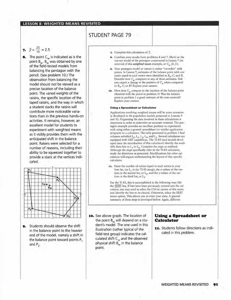
LESSON 8: WEIGHTED MEANS REVISITED
.;_ 25 7. y = 10 = 2.5
8. The point Cw is indicated as is the point Bw. Bw was obtained by one of the field-tested models from balancing the pentagon with the pencil. (See problem 10.) The observation from balancing the model should not be viewed as a precise location of the balance point. The varied weights of the raisins, the specific location of the taped raisins, and the way in which a student stacks the raisins will contribute more noticeable variations than in the previous hands-on activities. It remains, however, an excellent model for students to experiment with weighted means as it visibly provides them with the anticipated shift in the balance point. Raisins were selected for a number of reasons, including their ability to be squeezed together to provide a stack at the vertices indicated.
7 P1
-r--,__ ,_ I--. i-..
P2' Cw•~ ' Bw ' "' 8 ' P311t
I/ /
Ps'- ,__ ~
r-. -~
v .-- l<i P4 - 7
9. Students should observe the shift in the balance point to the heavier end of the model, namely a shift in the balance point toward points P1 and P2.
STUDENT PAGE 79
7, Complete this calculation of y. 8. Combine your results from problems 6 and 7. Mark on the
cut-out model of the pentagon constructed in Lesson 7 the centroid of this weighted mean example, or Cw (x, y).
9, Your pentagon model or cutout is rather "crowded" with points. In Lesson 7, estimates of the balance point with one raisin taped to each vertex were identified as B4, C, and B. Describe how Cw compares to any of these estimates. Did you expect a change in the position of Cw when compared to B4, C, or B? Explain your answer.
10. How does Cw compare to the location of the balance point obtained with the pencil in problem 1? Was the balance point in problem 1 a good estimate of the new centroid? Explain your answer.
Using a Spreadsheet or Calculator
Applications involving weighted means will be more extensively developed in the population models presented in Lessons 9 and 10. Organizing the data involved in these calculations is important in order to determine an accurate centroid. The pentagon example provides an excellent problem to experiment with using either a general spreadsheet (or similar application program) or a calculator. The table presented in problem 3 had columns subtitled L1, L2, L3, L4, and LS' Several calculators are equipped with LIST capabilities. The TI-83 (and models developed since the introduction of this calculator) identify the available data lists as L1 to L6. Complete the steps as outlined. · Although the steps specifically refer to the TI-83 calculator, study the directions as presented. Modifications for other calculators will require understanding the layout of that specific calculator.
11. Enter the number of raisins taped to each vertex in your first list, (or L1 in the TI-83 setup), the x-values of the vertices in the second list, or L2, and the y-values of the vertices in the third list, or L3'
For the TI-83, this is accomplished in the following way: Hit the ISTATI key. If lists have been previously entered into the calculator, you may need to select the ClrList option of this menu and identify the lists to be cleared. Otherwise, select the EDIT menu option. This allows you to enter your data. A general summary of these steps is developed below. Again, different
a. See above graph. The location of the point Bw will depend on a student's model. The one used in this illustration (rather typical of the field-test group) indicates the calculated shift Cw and the observed physical shift Bw in the balance point.
Using a Spreadsheet or Calculator
11. Students follow directions as indicated in this problem.
WEIGHTED MEANS REVISITED 91
LESSON 8: WEIGHTED MEANS REVISITED
STUDENT PAGE 80
IZ. Again, students follow directions as indicated in this problem. The values observed in the lists should be similar to what students recorded in Problem 3. Developing formulas through this process is very important as it demonstrates the calculator's ability to make many calculations needed in this problem. This becomes very important as students move to the next section and the greater number of data items and calculations.
92 LESSON 8
calculators will require a modified process in developing lists of the data.
If you need to clear the data from the lists, then ..
~ Clrlist I ENTER I
Clrlist Li,Li,L3,L\,Ls,L6 IENTERI
~ EDIT enter data as indicated in the appropriate list columns
If it is not necessary to clear the lists, then , •.
~EDIT enter data as indicated in the appropriate list columns
(Note: to back up, start over, or re-enter the data, you might need to return to the beginning of this process. To start again, hit~ IMODEI. The~ key indicates the command written on top of the raised IMODEI key will be executed or entered. In this case,~ IMODEI indicates the [QUIT] instruction will be executed. This instruction clears the screen and allows you to return to the ISTATI options, or, to re-enter the EDIT option of LISTS.
:iz. If the data is correctly entered in lists Lp L2, and L3, you are now ready to "program" the weighted values into your fourth and fifth lists, L4 and Ls- This can be done in different ways. One of the options available for the TI-83 involves the following:
With the lists visible in your window, use the arrow keys, If] and I!], to move the cursor to the top of L4 . If successful at this point in the process, L4 will be highlighted. The bottom of the screen should display:
L4 =
Using~ 1, and so forth, enter the following formula for L4:
L, *L, I ENTER I
This formula multiplies the number of raisins and the x-coordinate values for each point. Specific values should now be displayed in the L4 list.
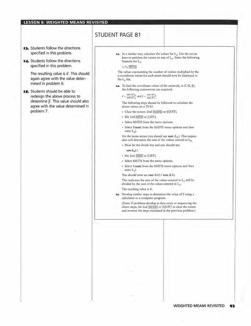
LESSON 8: WEIGHTED MEANS REVISITED
STUDENT PAGE 81
•~· Students follow the directions specified in this problem.
•4· Students follow the directions specified in this problem.
The resulting value is x. This should again agree with the value determined in problem 6.
•S· Students should be able to redesign the above process to determine j/. This value should also agree with the value determined in problem 7.
1:t. In a similar way, calculate the values for Ly Use the arrow keys to position the cursor on top of Ly Enter the following formula for Ls:
L1 •L3 IENTERI
The values representing the number of raisins multiplied by the y-coordinate values for each point should now be displayed in the Ls list.
14. To find the coordinate values of the centroid, or C (x, ji), the following summations are required:
X = sum of L4 and _ = sum of L5 sum of L1 Y sum of L1
The following steps should be followed to calculate the above values on a TI-83.
Clear the screen: 2nd IMODEI or [QUIT].
Hit 2nd ISTATI or [LIST].
Select MATH from the menu options.
Select S:sum( from the MATH menu options and then enter L4).
On the home screen you should see sum (L4 ). This expression will determine the sum of the values entered in L4 •
Now hit the divide key and you should see:
sum (L4 ) / ,
Hit 2nd ISTATI or [LIST].
Select MATH from the menu options.
Select S:sum( from the MATH menu options and then enter L1).
You should now see sum (L4) I sum (Ll) .
This indicates the sum of the values entered in L4 will be divided by the sum of the values entered in L1.
The resulting value is x. 15. Develop similar steps to determine the value of y using a
calculator or a computer program.
(Note: if problems develop in data entry or sequencing the above steps, hit 2nd !MODEi or [QUIT) to dear the screen and re-enter the steps explained in the previous problem.)
WEIGHTED MEANS REVISITED 93
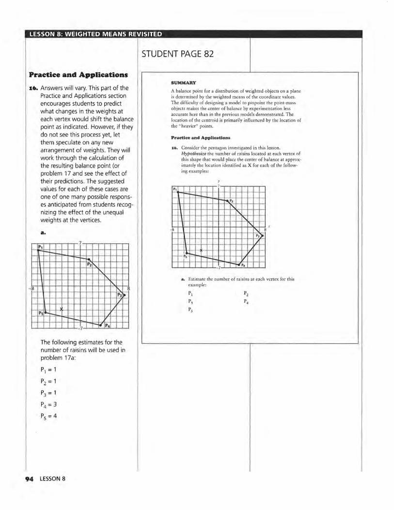
LESSON 8: WEIGHTED MEANS REVISITED
Practice and Applications
16. Answers will vary. This part of the Practice and Applications section encourages students to predict what changes in the weights at each vertex would shift the balance point as indicated. However, if they do not see this process yet, let them speculate on any new arrangement of weights. They will work through the calculation of the resulting balance point (or problem 17 and see the effect of their predictions. The suggested values for each of these cases are one of one many possible responses anticipated from students recognizing the effect of the unequal weights at the vertices.
--8
a.
7 P1 ,.._ ,__ ....__
,_ t-- r-.
P2f'.
" I-I-I-
I'. I'.
" P31)t
I/ I
P5 .._ ...._ -- '/
- 7 -I" P4
The following estimates for the number of raisins will be used in problem 17a:
P1 = 1
P2 = 1
P3 = 1
P4 = 3
P5 = 4
94 LESSON 8
STUDENT PAGE 82
SUMMARY
A balance point for a distribution of weighted objects on a plane is determined by the weighted means of the coordinate values. The difficulty of designing a model to pinpoint the point-mass objects makes the center of balance by experimentation less accurate here than in the previous models demonstrated. The location of the centroid is primarily influenced by the location of the "heavier" points.
Practice and Applications
1&. Consider the pentagon investigated in this lesson.
Pt
Hypothesize the number of raisins located at each vertex of this shape that would place the center of balance at approximately the location identified as X for each of the following examples:
y
--"--
'" I '"' , 1'- x
. ," 8
I
\ , .__ - ~~-t.._-'1'-1-..:±--t--l--t-i-t-t-Tl-v-t--t--I
I 1""-t-.. /
a. Estimate the number of raisins at each vertex for this example:
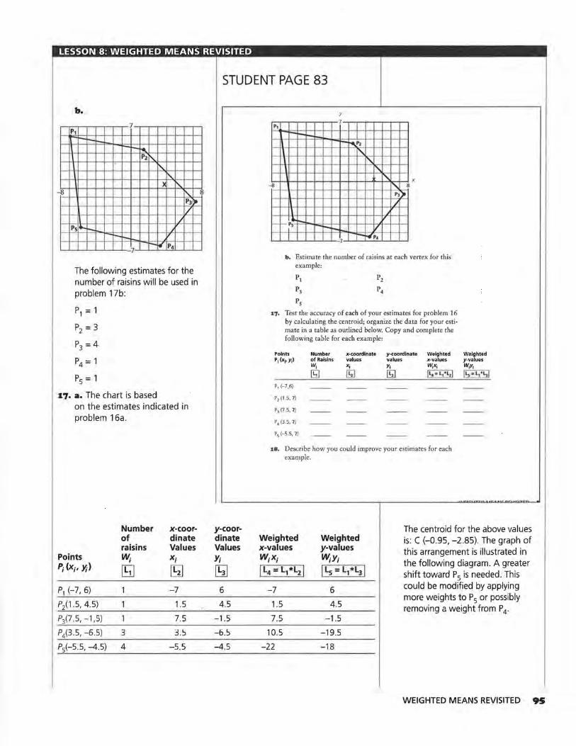
LESSON 8: WEIGHTED MEANS REVISITED
STUDENT PAGE 83
b.
7 P1
r---- -~ P21'\. .
I'\.
' ) ' I'\. P3 ~
I/ /
Ps .._ ,_ j -- , r- !If" P4
7
The following estimates for the number of raisins will be used in problem 17b:
P1 = 1
P2 = 3
P3 = 4
P4 = 1
P5 = 1
17. a. The chart is based on the estimates indicated in problem 16a.
Number x-coor-of dinate raisins Values
Points W; X; P; (X;, )1) [SJ [5]
P1 (-7, 6) -7
P2(1 .5, 4.5) 1.5
Pp.5, -1,5) 7.5
P4(3.5, -6.5) 3 3.S
P5(-5.5, -4.5) 4 -5.5
y-coor-dinate Values Y; [5J
6
4.5
-1.5
-6.S
-4.5
y
,_ __ 1--1++-t--+--l-+-t-t--t--t-l'\.,,,.,. __ l--t-t-+---t
' I'\ x
-s- 1--+-1--+--1-1-1-1.-1--1--+-+-1-1-'-,,_,3 PJ")
\ r--P~.-F-"'!--.....C--f-l-f--t--1-+VY!-~-l--t-I ... ~~
b, Estimate the number of raisins at each vertex for this example:
pl
P3
Ps
'-7· Test the accuracy of each of your estimates for problem 16 by calculating the centroid; organize the data for your estimate in a table as outlined below. Copy and complete the following table for each example:
P1 (-7,6)
P2 (1 5, 7)
P3 (7 5, 7)
P.<3.5, 7)
P5 (-5,5, 7)
Number of Raisins w, [SJ
x-coordinate values x, I!!]
y-coordinate values Y1
[Q
Weighted x-values W1X1
IL .. • L,·L1]
J.8. Describe how you could improve your estimates for each example.
Weighted y-values w,y, Ii..# Li ' li l
The centroid for the above values Weighted Weighted is: C (-0.95, -2.85). The graph of x-values y-values this arrangement is illustrated in W;X; W;Y; [ L4 = L1•L2 j I Ls= L, *~ I
the following diagram. A greater shift toward P5 is needed. This
-7 6 could be modified by applying
1.5 4.5 more weights to P5 or possibly removing a weight from P4 .
7.5 -1 .5
10.5 -19.5
-22 -18
WEIGHTED MEANS REVISITED 95
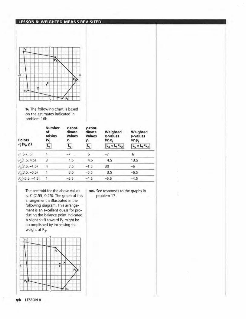
LESSON 8: WEIGHTED MEANS REVISITED
7 P1
r---- - r--~ P21'\_
:"\.
' I'\. I'\. 8
P3 • c I/
' I Ps.._ ...... J -- /
r-- i.r P4 7
b. The following chart is based on the estimates indicated in problem 16b.
Number x-coor-of dinate raisins Values
Points W; X; P; (x;,Y;) [5] ~ P1 (-7, 6) 1 -7
P2(1.5, 4.5) 3 1.5
Pp.5, -1,5) 4 7.5
P4(3.5, -6.5) 3.5
?5(- 5.5, -4.5) -5.5
The centroid for the above values is: C (2.55, 0.25). The graph of this arrangement is illustrated in the following diagram. This arrangement is an excellent guess for producing the balance point indicated. A slight shift toward P3 might be accomplished by increasing the weight at P3 .
7 P1
- ... -..._ ..._ --"' ,_ - P2'-~
\.. . )( ' 8 c I'\. P3 )t I/
I Ps..._ ...... /
:--- /
7 -19' P4
96 LESSON 8
y-coor-dinate Weighted Weighted Values x-values y-values Y; W;X; W;Y;
[5J I L4 = L,*L2 [ JL5 =L1*L3 J
6 -7 6
4.5 4.5 13.5
-1.5 30 -6
-6.5 3.5 -6.5
-4.5 -5.5 -4.5
i:s. See responses to the graphs in problem 17.
UNIT IV
Population Centers

LESSON 9
Finding a Population Center Materials: No additional materials are required for this lesson.
Technology: graphing calculator Pacing: 2 to 3 class sessions
Overview
Lesson 9 moves the center determined by a centroid to a population center. The models developed with raisins and poster paper (heavier paper) are now representing people and locations on a map. Although the students have studied a center of balance by investigating shapes, the significance of this center is probably still unclear. This lesson involves a map of six communities in southeastern Wisconsin. Each community represented is compared to a vertex in the polygon model of Lesson 8. The population of the communities is similarly compared to the number of raisins taped to each vertex of the polygon model. If a physical model of this map was constructed based on the previous lesson, then a student would create a stack of raisins representing the population of each community on a cut out map of the region. Obviously stacks of raisins representing populations is no longer workable, therefore, the connection of a balance point to a centroid is used to estimate a population center.
The importance of the population center in Lesson 9 is. built around the idea of "fairness." By balancing distance and population, a population center represents a location that is fair to the people represented in the region. In a social context, the population center is a way to balance the issues of distance and the number of people.
Teaching Notes
Both this lesson and Lesson 10 are different in style and content from the previous lessons in this module. This is intentional as the focus of the lessons is to bridge the development of the geometric models into specific applications. Although there are several other ~pplications that could have been developed, connectmg a center of balance to a population center is a way to connect balance in a social context. (The physical science connections were hopefully implied through the earlier lessons of this module.) A range of questions are developed in the text, however, the field test teachers particularly commented about the interesting discussions and questions related to this topic that were not anticipated.
Technology
This lesson is dependent on use of a calculator or a computer. Without these tools, students will be frustrated. This lesson can be handled by a calculator with LIST options as outlined in the previous lessons. The charts used to support the organization of data needed to complete this lesson follow the model of a TI-83 graphing calculator. Specifically, the six lists needed to calculate the population center are labeled accordingly. Modifying this for other types of calculators or to a computer spreadsheet should not be difficult given the data represented in each list. Exploring
FINDING A POPULATION CENTER 99
se¥eral of the "What if ... ?" questions related to the nature of this lesson would certainly be enhanced by a spreadsheet application or by a calculator with linked list options (for example, a TI-83 or similar product).
Follow-Up
The problems suggested in this lesson are studied in colleges and universities as part of several disciplines. Most notably, several urban centers (similar to Milwaukee, mentioned in the map displayed in this lesson) have universities involved in the study of urban planning. Contact a large university and determine if it has a degree program or a department involved in the estimation of population studies and planning. The opportunity for this type of contact can be investigated by organized searches through the Internet.
IOO LESSON 9
LESSON 9: FINDING A POPULATION CENTER
STUDENT PAGE 87
LESSON 9
Finding a Population Center
Suppose there are people, instead of raisins, located at the vertices of a very large pentagon. Would your method change for finding the center of balance?
Why might this center of balance, or population center, be important?
What type of questions does the location of a population center answer?
T he balance point models developed in the previous lessons assumed the weight of each raisin (or object) was equal. If
several raisins were located at each vertex, then a weighted mean was calculated. This equalizes the effect of each raisin on the balance of the objects.
A population center has a similar interpretation. Instead of balancing the weight of objects related to distance, however, a population center balances the "number of people" related to distance. A population center gives "equal status" to each person based on his or her location on a plane. It represents the location where the number of people and their respective distances are balanced. This lesson and Lesson 10 attempt to develop and explain the significance of a population center.
INVEST IGATE
Population Centers
A population center is the "balance point" of a distribution of people. Population statistics are extensively studied and analyzed at the local, national, and global level. The United States Constitution directs that an actual count of the citizens of this
Interpret a population center as a measure of
balance.
Set up and calculate a population center.
Interpret a population center as an average of location and population
Describe the appropriate-ness of applying a
population center to a real-world problem .
FINDING A POPULATION CENTER IOI
LESSON 9: FINDING A POPULATION CENTER
STUDENT PAGE 88
XOZ LESSON 9
country must be made every 10 years. The Bureau of the Census is the designated agency to carry out a U.S. census at the start of each decade. Each completed census provides volumes of data to interested citizens and political groups.
Di11CUSslon and Practlae
Pretend you are an important political person back in the 1980s. You are appointed by the Governor of Wisconsin to head a committee to determine the location of an important job service agency in that state. You and your committee are responsible for helping the people residing in the communities of Milwaukee, Waukesha, Port Washington, Belgium, Beloit, and Racine. A map of this area of Wisconsin is provided below. Also included in this sketch are the 1980 population statistics that the committee will use in making a decision. The recommendations of your committee are expected to service the people of this area for at least the next 20 years. A review of your decision will be made in 1990 and again in 2000. You have an
Population based on 1980 Census
Beloit 35,207 •
• Waukesha 50,365
Source: 1980 U.S. Department of Commerce, Bureau of the Census
• Belgium 892
LESSON 9: FINDING A POPULATION CENTER
Solution Key
Discussion and Practice
1. Answers will obviously vary at this point. Most students in the fieldtest group indicated they would locate the agency between Waukesha and Milwaukee. Their explanations included locating the agency closest to most of the people represented in the map, finding a "central" geographical location, and balancing the extreme locations of Belgium and Racine.
z. a. Most of the people in the region would be traveling to an extreme southwest location.
b. More of the people represented in the map would be traveling to an extreme location to the north. Also, Belgium has the smallest number of people; locating the agency in Belgium would require most of the people to travel.
c. Most of the people in the map would be traveling to an extreme southeast location.
(Note: An additional challenging question would be to ask if locating the agency in Milwaukee would be fair. Students sense it represents a good location for most of the people, however, they also feel uncomfortable placing the agency in any of the specific cities. It represents a good discussion question for setting up the rest of this lesson.)
STUDENT PAGE 89
interest in running for governor at some future date and feel this appointment is an opportunity to demonstrate your leadership skills.
:t. Describe at least three factors you and your committee should consider in making a determination concerning the location of the job service agency.
2. Representatives of the six communities identified as the primary recipients of this service might recommend that the agency be located in their respective communities.
a. Explain why a decision to locate the agency in Beloit might be "unfair."
b. Explain why a decision to locate the agency in Belgium might be considered "unfair."
c. Explain why a decision to locate the agency in Racine might be considered "unfair."
~. If the advisory group attempts to base their decision on fairness to the people located in these communities, what factors d.o you think are most critical to consider?
Locating a Population Center
The general location of each community is identified on the following map by a point. The collection of the communities (or points) resembles the model of a polygon. Replacing the number of raisins at each vertex with the number of people counted at each community allows you 'to begin thinking about a balance point. As the population of each community is not equal, calculating a balance point or population center would be similar to the model developed in Lesson 8 for weighted means.
~. "Fairness" is a very difficult concept to define; this question could spark an interesting debate. Issues of fairness are very complex and involve many factors not mentioned in problems of this type. Given the data, however, students will probably highlight that fairness seems to be related to distance and the number of people involved in the represented region .
FINDING A POPULATION CENTER 103
LESSON 9: FINDING A POPULATION CENTER
STUDENT PAGE 90
Locating a Population Center
4. The following values approximate the locations.
x-coordinate y-coordinate Community value value
Belgium 5.3 6.2
Port Washington 4.8 4.5
Waukesha 2.3 1.7
Milwaukee 5.0 1.7
Beloit -1.5 -2.1
Racine 6.3 -1.5
I04 LESSON 9
Consider calculating a population center by placing a coordinate grid over the map below:
... eels1!n
I I 6
I I ~9i I Population based on 1980 Census Port Washington /
! 8,612. (
~ '-''\ v,., •• ~. ~ ~6.,236
2
l.J ~==~ Waukesha 50,365 -
\ LI
__ j, -3
I I l\. -2 2 4 -Racine 85,725
(_ Beloit 35,207 ·- -2 u I
Source: 1980 US Department of Commerce, Bureau of the Census
4, Based on this particular coordinate grid, determine approximate x and y values for each of the communities.
x-coordlnate y-coordinate Community value value
Belgium
Port Wash
Waukesha
Milwaukee
Beloit
Racine
I ---
--·
LESSON 9: FINDING A POPULATION CENTER
STUDENT PAGE 91
s. The values for the last two columns, P;x; and P;Y;, have been rounded to the nearest integer values. (See table at the bottom of this page.)
6 6. a. LP; represents the sum of the
Cs)
i =1 populations of the six cities represented in this region,
5 LW; represents the sum of the i =1 raisins from each vertex of the pentagon. In effect, we are equating "population" to the "number of raisins."
6 It. LP;<; represents the sum of
i =1 the products of each population times its location. (Or in this case, it represents the sum of the products of each city's population times its x-coordinate.)
5 LW;<; represents the sum of the i =1 products of the number of raisins at each vertex times the corresponding x-coordinate in the pentagon model.
Popu- x-lation coordinate
Community P; value (x;}
Belgium 892 5.3
Port Washington 8,612 4.8
Waukesha 50,365 2.3
Milwaukee 636,236 5.0
Beloit 35,207 -1.5
Racine 85,725 6.3
y-coordinate value (y;}
6.2
4.5
1.7
1.7
-2.1
-1.5
s. A population center organizes the population and coordinate values of the communities in the same way the weights and coordinate values of the raisins were organized in Lesson 8. Copy and complete the following chart to determine the population center. (Note: use of a calculator or spreadsheet is encouraged but not required.)
Population x-coordinate y-coordinate Community p, value (x.) value (y1) P;X;
Belgium 892
Port Wash 8,612
Waukesha 50,365
Milwaukee 636,236
Beloit 35,207
Racine 85,725
lo. The population center is described by the following weighted means:
6 6
LPixi LP;Yi
x = J=1_ and y = J=1_ 6 6
~>, LP, . i=1 i=1
6 5
L~ · L~ a. What does i=l represent? (Compare this to i=l in the
pentagon model developed in the previous lesson.) 6 5
LPix1 Lwixi b. What does i=l represent? (Compare this to i=l in
the pentagon model.)
7. Complete the calculations to determine the population center, or P (:X, y), for the map provided.
s. Does the location suggested by problem 7 seem to be a "fair" location for the job service agency? Why or why not?
Will the design or placement of a specific coordinate grid change the location of the population center?
7. P (.X, fl is approximately P (4.7, 1.2).
f';X; P; Y; 8. In most discussions, the students indicated the above location is fair.
4,728 5,530 This location seems to balance the distance and population values for
41,338 38,754 the region represented by this
115,840 85,621 map.
3,181,180 1,081,601
-52,811 -73,935
540,068 -128,588
FINDING A POPULATION CENTER ~OS
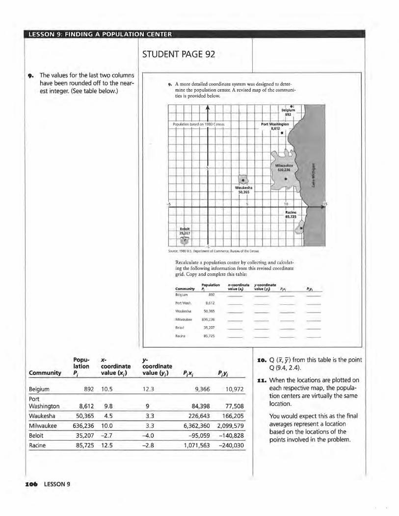
LESSON 9: FINDING A POPULATION CENTER
9. The values for the last two columns have been rounded off to the nearest integer. (See table below.)
Popu- x-lation coordinate
Community P; value (x';)
Belgium 892 10.5
Port Washington 8,612 9.8
Waukesha 50,365 4.5
Milwaukee 636,236 10.0
Beloit 35,207 -2.7
Racine 85,725 12.5
~06 LESSON 9
STUDENT PAGE 92
y-
9, A more detailed coordinate system was designed to determine the population center. A revised map of the communities is provided below.
+ 1 •1 -!} Belgium 892 I I
Population based on 1980 Census Port Washington(' 8,612
• l:.
-I'.\. __ /
5 Ml""~u~eo 6~6;J:36 . ) \ •
Waukesha :'.:_/'1V'"r\ J 50,365
I - 1
5 110 "-... kaclne ~ 85.725 -
~'
BE olt 35 207 -~
~ 5
Source: 1980 U.S Department of Commerce, Bureau of the Census
Recalculate a population center by collecting and calculating the following information from this revised coordinate grid. Copy and complete this table:
Population x-coordinate y-coordinate Community P1 value (x1) value (y1) Plxi
Belgium 892
Port Wash. 8,612
Waukesha 50,365
Milwaukee 636,236
Beloit 35,207
Racine 85,725
l · -,
t J
J'1s -
IO. Q (x, fl from this table is the point coordinate Q (9.4, 2.4). value (y;) P;X; P;Y;
••· When the locations are plotted on 12.3 9,366 10,972 each respective map, the popula-
tion centers are virtually the same
9 84,398 77,508 location.
3.3 226,643 166,205 You would expect this as the final
3.3 6,362,360 2,099,579 averages represent a location
-4.0 -95,059 -140,828 based on the locations of the points involved in the problem.
-2.8 1,071,563 -240,030
LESSON 9: FINDING A POPULATION CENTER
12. This problem returns to the issue of "fairness." If the primary factors used in evaluating fairness are location and the number of people, then the population center identified by this process attempts to consider both factors in a fair way.
1~. The data for Belgium was omitted from this table. A typical reaction to this is that it is not fair. An "unfair" judgment, however, is based on criteria other than population and location as the remaining problems attempt to point out. Remind students, however, "fairness" is a very complex and an open-ended standard; it is a goal that cannot realistically be defined by this type of problem. This problem is intended to point out the complexity of this concept.
14. As either grid is okay to use in this problem, the following data was collected from the second grid. (Recall values are rounded to the nearest integer in the last two columns.)
Popu- x-lation coordinate
Community P; value (x;)
Port Washington 8,612 9.8
Waukesha 50,365 4.5
Milwaukee 636,236 10.0
Beloit 35,207 -2.7
Racine 85,725 12.5
STUDENT PAGE 93
y-
10. Determine the population center Q (x, ji), from this table.
11. Compare the locations of the two population centers derived from each example, P and Q. Would you expect the centers to be similar? Why or why not?
iz. If the population center were to be suggested as the location of the agency, do you think each community would consider this recommendation "fair"? In what way does the population center approach seem to address some of the concerns of fairness?
The "Belgium Problem"
An incomplete table of the populations of the communities involved in this decision was developed. Consider the following incomplete table:
Population x-coordinate y-coordinate Community P; value (x1) value (y;l P1x1
Port Wash. 8,612
Waukesha 50,365
Milwaukee 636,236
Beloit 35,207
Racine 85,725
13. What data were omitted from this table? Is this fair?
14. Determine a population center for the five communities listed in this incomplete table. Use either the first or the second grid to complete the x- and y-coordinate values for each community.
15. Compare the population center derived from this incomplete table with the center derived when all six communities were considered. How does the incomplete data table change the recommendation of the advisory group?
16. Describe what you think is meant by the title of this investigation "The Belgium Problem."
17. Consider the omission of the city of Milwaukee data from the table listing the six communities. Would this omission change the location of the center of the population? Estimate where the center of population would be located if the city of Milwaukee were not considered in the population distribution.
coordinate 15. Comparing the population center
with the Belgium data to the population center without Belgium does not make any difference. Belgium's very small population (when compared to the other cities in this problem) contributes little to the population center.
value CY;) P;X; P;Y;
9 84,398 77,508
3.3 226,643 166,205
3.3 6,362,360 2,099,579
-4.0 -95,059 -140,828
-2.8 1,071,563 -240,030
The population center P (x, fl based on the data from the five cities is P (9.4, 2.4).
16. Essentially the "Belgium Problem" refers to the minor contribution Belgium plays in the location of the population center of this region. This is a good time to summarize exactly what is critical in the calculation of a
FINDING A POPULATION CENTER ~07
LESSON 9: FINDING A POPULATION CENTER
population center, namely, location and number of people. If the number of people of a city is minor compared to the other cities, then the only way this city influences a population center is through a location very far from the other cities. As this is not the case, Belgium has little influence in the calculation of the population center.
x7. Omitting Milwaukee from the data is far more critical than Belgium . As the number of people is greater than any of the other cities, Milwaukee has the greatest pull in determining the population center of this region. If Milwaukee was dropped from the chart, then the location of the population center for the five remaining cities would be P (7.2, -0.7) using the second coordinate grid illustrated in this lesson . As you study this location on the map, notice how the population center shifts in the direction of the next largest city. Notice also how the locations of the other large cities (i.e .. Waukesha and Beloit) have a "pull" on this new population center.
(Note: Another challenging question is to speculate on the role of Belgium in the problem if Milwaukee were excluded. Has Belgium increased its contribution to the location of the population center? Have students speculate on that question and how they would test it out. It is anticipated students would examine the population center vvith and vvithout Belgium to answer that question . Belgium, however, still does not influence the population center.)
Practice and Applications
I.8. Using the second grid and the 1990 Census of the six communities, the following data would be recorded for this region:
108 LESSON 9
STUDENT PAGE 94
SUMMARY
The population center represents a location balancing the number of people and their respective locations. Each person is considered "equal" in the calculation of this center. Similar to the previous study of a balance point, the location of the population center is influenced by a region's specific populations and their respective locations.
Practice and Applications
I8. Evaluating your 1980 decision is important! The 1990 Census of the six communities studied in this lesson is provided in the following table. Copy the table below. Use one of the two coordinate grids to help you complete this table.
Population x-coordinate y-coordlnate Community P, value (x1) value (y1) P1X1
Belgium 1,405
Port Wash. 9.338
Waukesha 56.958
Milwaukee 628,088
Beloit 35,573
Racine 84,298
I9. Before calculating the revised population center using the 1990 population figures, estimate the location of the 1990 population center as a coordinate point on the grid.
Explain what factors you ~onsidered in making your estimate.
zo. Based on the 1990 population figures, determine the population center P (x, y).
21. Describe how the population center changed from 1980 to 1990.
If the location of the job service agency were based on the 1980 populations, would the six communities be similarly served by the agency in 1990? Explain your answer. Was your 1980 decision a good one?
zz. Consider the following investigations. For each item, explain whether or not a population center would be
Popu- x- y-lation coordinate coordinate
Community P; Value (x;) Value (y;) P;X;
Belgium 1,405 10.5 12.3 14,753
Port Washington 9,338 9.8 9.0 91,512
Waukesha 56,958 4.5 3.3 256,311
Milwaukee 628,088 10.0 3.3 6,280,880
Beloit 35,573 -2 .7 -4.0 -96,047
Racine 84,298 12.5 -2.8 1,053,725
P1Y1
17,282
84,042
187,961
2,072,690
-142,292
-236,034
LESSON 9: FINDING A POPULATION CENTER
19. This will be a difficult problem for the students! The major gains in population are Belgium (which previously did not influence the population center), Port Washington (also a small population city), and Waukesha. Population losses are noted in Milwaukee and Racine. Beloit shows a very small increase. As the location for each city remains the same, the conjecture of a new population center will probably describe a shift to the west or northwest.
zo. Based on the 1990 population figures, the population center P (x, y) is P (9.3, 2.4). This is a very slight shift to the west from the previous center.
z1. The results indicate little change in the center during the decade. The slight change to the west is probably explained by the increase in the population of Waukesha and the population declines of Milwaukee and Racine. Interestingly, this observation remains a very important factor in planning future service agencies for this area of Wisconsin.
Services for the six communities are well-serviced by the 1980 location as there is little change in the overall population center.
zz. a. Probably not a good example of using a regional population center. The congregation of the church, temple, or synagogue would possibly consider a population center of the people belonging to its organization, but this is probably very difficult to determine. Zoning, availability of land, and potential future growth are probably more important factors. Students might research this by contacting a governmental planning agency.
STUDENT PAGE 95
considered. In addition, indicate what other factors might be involved in each decision.
a. Location of a church or temple or synagogue for a large congregation.
b. Location of a school for a growing school district.
'" Location of a shopping mall for a suburban community.
d. Location of an airport to service three large cities.
e. Location of a large recreational facility (for example, a stadium for a major league baseball or football team).
f, Location of public housing units for the elderly.
z:t. Using a map of your state or geographic area, determine the population center for the three or four largest communities of interest to you or your class.
Z4· Locate Gurnee, Illinois, on a map of Illinois and Wisconsin. This small community is the location of a very large recreational park, Six-Flags Great America®. Why would a very small community be selected as the location for one of the largest amusement parks in the United States?
zs. Consider the previous map of the six communities involved in the investigations of this lesson. Someone hypothesized that it was possible for the center of population of the communities to be located in Lake Michigan! Could there be a population distribution of these six communities that would place the center of population in Lake Michigan? Explain your answer.
Before you complete this module, it is very important to more thoroughly understand a population center. For example, a population center is not the location that minimizes distances to a specific point for each of the people in the model. Although frequently close to this point, finding a location that minimizes distances represents another type of center. Stay tuned. Investigations in Lessons 11 to 13 will help you understand other types of centers.
b. Schools need to be located close to the students and to the future growth of a city. This represents a very difficult decision to make. (Many cities have made very poor choices by not considering factors of population growth or decline, locations of residents with children, income levels.) This is primarily a discussion problem that could be answered by considering a population center. In actuality, the issue is clearly more complicated than simply a population center.
c. A population center could be considered in this decision, however, other factors such as availability to freeways or airports, income levels, hotel facilities, future growth of city, availability of land for expansion, and other attractions are very important. Students could research the site selection of the Mall of America in Minneapolis to gain insight into a decision of this type. (A very fascinating and complex set of concerns were considered.)
FINDING A POPULATION CENTER I09
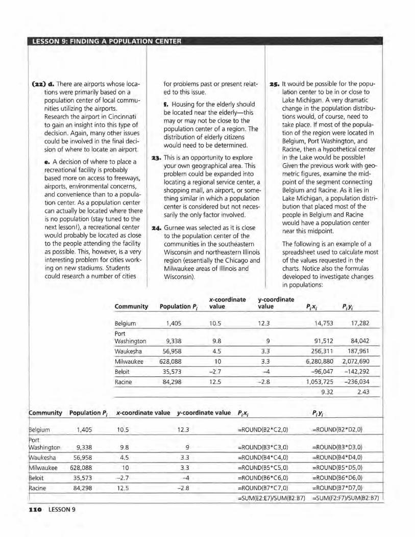
LESSON 9: FINDING A POPULATION CENTER
(22) d. There are airports whose loca- for problems past or present relat- 25. It would be possible for the popu-tions were primarily based on a ed to this issue. lation center to be in or close to population center of local com mu-
f. Housing for the elderly should Lake Michigan. A very dramatic
nities utilizing the ai rports. be located near the elderly-this
change in the population distribu-Research the airport in Cincinnati tions would, of course, need to to gain an insight into this type of
may or may not be close to the take place. If most of the popula-
decision. Again, many other issues population center of a region . The
tion of the region were located in could be involved in the final deci-
distribution of elderly citizens Belgium, Port Washington, and
sion of where to locate an airport. would need to be determined.
Racine, then a hypothetical center
e. A decision of where to place a 23. This is an opportunity to explore in the Lake would be possible!
your own geographical area. This Given the previous work with geo-recreational facility is probably
problem could be expanded into metric figures, examine the mid-based more on access to freeways,
locating a regional service center, a point of the segment connecting airports, environmental concerns,
shopping mall, an airport, or some- Belgium and Racine. As it lies in and convenience than to a popula-
thing similar in which a population Lake Michigan, a population distri-tion center. As a population center
center is considered but not neces- bution that placed most of the can actually be located where there
sarily the only factor involved. people in Belgium and Racine is no population (stay tuned to the
would have a population center next lesson!), a recreational center 24. Gurnee was selected as it is close near this midpoint. would probably be located as close to the population center of the to the people attending the facility communities in the southeastern The following is an example of a as possible. This, however, is a very Wisconsin and northeastern Illinois spreadsheet used to calculate most interesting problem for cities work- region (essentially the Chicago and of the values requested in the ing on new stadiums. Students Milwaukee areas of Illinois and charts . Notice also the formulas could research a number of cities Wisconsin) . developed to investigate changes
in populations:
x-coordinate y-coordinate Community Population P; value value P;X; P;Y;
Belgium 1,405 10.5 12.3 14,753 17,282
Port Washington 9,338 9.8 9 91,512 84,042
Waukesha 56,958 4.5 3.3 256,311 187,961
Milwaukee 628,088 10 3.3 6,280,880 2,072,690
Beloit 35,573 -2 .7 -4 -96,047 -142,292
Racine 84,298 12.5 - 2.8 1,053,725 -236,034
9.32 2.43
~ommunity Population P; x-coordinate value y-coordinate value P;X; P;Y;
3elg ium 1,405 10.5 12.3 =ROUND(B2*C2,0) =ROUND(B2 * D2,0)
)ort Nashington 9,338 9.8 9 =ROUND(B3 * C3,0) =ROUND(B3*D3,0)
Naukesha 56,958 4.5 3.3 =ROUND(B4*C4,0) =ROUND(B4 *D4,0)
\i1ilwaukee 628,088 10 3.3 =ROUND(B5*C5,0) =ROUND(B5* D5,0)
3eloit 35,573 -2 .7 -4 =ROUND(B6*C6,0) =ROUND(B6*D6,0)
Racine 84,298 12.5 -2 .8 =ROUND(B7*C7,0) =ROUND(B7*D7,0)
=SUM(E2:E7)/SUM(B2:B7) =SUM(F2:F7)/SUM(B2:B7)
IIO LESSON 9
LESSON 10
Finding the Population Center of the United States Materials: Activity Sheets 8-12, Unit IV Quiz
Technology: graphing calculator
Pacing: The number of class sessions will vary depending upon
the format selected for completing this project.
Overview
This lesson opens up the study of a population center to the larger goal of estimating the population center of the United States using the 1990 Census data. The importance of this location as studied by previous locations of the United States' mean population center are sited in the text. This lesson involves a similar process to the work presented in Lesson 9, however, it expands significantly the organization and impact of the process. This is an excellent miniproject to conclude the group of lessons that started with Lesson 3.
Teaching Notes
There are several ways to complete the project discussed in the text. Essentially, the following options should be considered.
Option I One of the teachers in the field-test group organized small groups of three to four students to complete the "The Big Picture." Students were provided atlases to determine the location of state capitals. Each group developed their own coordinate system on the unmarked U.S. map (one of two maps provided with the masters), located the 48 state capitals, and completed the data sheet organized for the "The Big
Picture." (See Activity Sheets 8 and 12.) By developing this lesson through small groups, this project took three days to complete. (A considerable amount of time was related to the geography connections of locating capitals and learning information about the states!) This teacher was very satisfied with the results from the groups.
Optionz A coordinate map of the 48 connected states is provided as Activity Sheet 9. In addition, approximate locations of each state capital are provided. This map can be presented to students. Estimating the population center involves recording the x- and y-coordinates for each state's capital and completing the population charts as outlined for this project. This option saves considerable time in locating the capitals. It also provides a check on the accuracy of students' estimates of the xy-coordinates. This work could also be developed through small groups.
Option :5 A partially completed data recording sheet is provided as Activity Sheet 10. This sheet includes the coordinate values for each state's capital as illustrated by the coordinate map described in Option 2. Students are still expected to complete the chart as outlined in the text. Although some tedious calculations still remain,
FINDING THE POPULATION CENTER OF THE UNITED STATES III
use of the activity sheets will decrease the time needed to complete this version of the project. (Essentially the connections to geography topics are less developed with this option.)
The significance of the population center is important regardless of which option is selected. Compare the students' estimates of the population center to the results reported by the Bureau of the Census. (Again, Activity Sheet 12 is provided to indicate the 1990 population center and some background information on this location. Interesting information about Crawford County, Missouri, can also be located on the Internet!). This is an interesting lesson to develop and an interesting lesson for discussion. Developing this project with a U.S. history or geography class was viewed by one of the field-test teachers as an especially exciting extension for both classes.
Technology
If the development of a center involves all of the states, then a spreadsheet application may be required. (The memory of a graphing calculator might be too small to handle this volume of data. Check the specifications of your calculators!)
Follow-Up
A historical study of the locations of several state capitals can be related to estimating a city best representing a state's mean population center. A research of the capitals (through the Internet and through general geography and history reference books) would probably indicate the significance of this type of center in history.
IIZ LESSON 10
LESSON 10: FINDING THE POPULATION CENTER OF THE UNITED STATES
Solution Key
Discussion and Praetiee
1.. This shift to the west can be explained by the expansion of the country in that direction. A lot of history can be seen in the shifts of the population centers. Land purchases and westward migration are the most obvious explanations for this shift.
STUDENT PAGE 96
LESSON 10
Finding the Population Center ol the United States
Do you think you could compute the population center of the entire United States?
Would you expect the population center of the U.S. in the year 1775 to be the same as the population center of the U.S. in the year 1850? Why or why not?
. : Calculate a population center based on coordinate points and census
populations.
Hypothesize population changes and the effects
on the population center.
T he population center for the six communities in southeastern Wisconsin was a manageable extension of the polygon
models. Expand on this idea even more by imagining that you are in outer space looking down at the entire United States. Instead of viewing a small section of one state, you are now looking at an entire country! Where do you think the population center for the United States is currently located?
INVESTIGATE
Westward, Ho!
The U.S. Bureau of the Census determines the population center of the United States from the census data collected at the beginning of each decade. The map on the next page plots the population centers for each decade from 1790 to 1980, as determined by the Bureau of the Census. Consider how the population center of the United States has shifted over the years.
Discussion and Practice
1. The population centers have consistently moved westward. Explain this westward shift in the population center.
FINDING THE POPULATION CENTER OF THE UNITED STATES II~
LESSON 10: FINDING THE POPULATION CENTER OF THE UNITED STATES
2. The migration to the south is due to many factors, including climate, aging of the population (the migration of older people to warmer climates), labor conditions, and the influx of citizens from Mexico into the southwestern regions of the country.
~. Most predictions are based on continued shifts to the west and south for the same reasons mentioned in problem 2.
4, a. Westward movement due to the expanding access to this area of the country. (The Oregon Trail and other access routes were opening up this area of the country.)
b. The expansion and inclusion of the western states. (Actual states were admitted to the country during this time.)
c. Labor and climate issues that resulted in numbers of people moving to the west and south at the expense of the "rust" belt regions.
d. The shift noted here is partially due to the inclusion of Alaska and Hawaii into the calculation of the population center.
II4 LESSON 10
STUDENT PAGE 97
:t. Jn addition to a westward shift, the population centers have also indicated a trend to the south, especially since 1910. What are your ideas on the gradual shift to the somh an<f west?
~. Your goal in this lesson is to approximate the center of population for 1990. The location of this center as determined by the 1990 Census will be shared with you at the conclusion of this lesson . Based on the centers presented in the above map, where do you think the 1990 population center was located? Why did you select this location?
Source: The Statistical Abstract of the United Stares, 1991
4, Some decades indicate a greater shift of the country's population center than other decades. Investigate what historical events highlight the following decades that might explain the greater shifts in the population noted on the map:
a. 1870-1880
b. 1900-1910
"· 1970-1980
d. 1950-1960
s. As previously explained in Lesson 9, the population center is a measure that "equalizes" people based on their relative locations on the map of the United States. The population
'counts that were used in determining the population center were based on the results from the Bureau of the Census for
LESSON 10: FINDING THE POPULATION CENTER OF THE UNITED STATES
5. a. The Census Bureau has particular difficulty in counting all the people in large urban areas. There is some serious discussion that figures from the Census need to be adjusted. This was determined from sampling studies that investigated the low number of people counted in these areas. It is particularly interesting to point out to students that the Census numbers are very important in determining representation in Congress and the distribution of federal money.
b. Early census counts did not take into account slaves, Native Americans, and probably poor populations. It is impossible to determine exactly how many people were involved in this "under count."
c. As indicated in b, slaves, Native Americans, and the poor were not represented at that time. Questions exist as to whether or not women were adequately counted during some of this time.
6. Thomas Jefferson was the first president inaugurated in Washington DC in 1801. At that time, Washington was close to the estimated population center of the country (see the map from the Census Bureau). Shortly after Jefferson became president, however, our country purchased the Louisiana Territory. This purchase dramatically changed the population center and the future distribution of the population of our country for years to come.
7. a. Alaska and Hawaii are not connected to the rest of the states of the country. The 48 states are frequently called the 48 connected states. The distance of Hawaii from the mainland is particularly impressive-thousands of miles!
STUDENT PAGE 98
each decade. Based on your understanding of the census, consider the following questions.
11, Do you think the Bureau of the Census is currently accurate in counting almost everyone in the country? Why or why not?
b. Do you think the Bureau of the Census was accurate in counting most of the people in the early decades of this map? Why or why not?
c. Describe people the Bureau of the Census might not have counted in the decades of 1790 to 1850.
•· Washington DC was a "planned city." The location of Washington DC was based on an honest attempt to identify a fair location for all the people in the country. Do you think the location of Washington DC was based on the population center of the country? Why or why not? (Research this question!)
How 11 the Population Center Determined?
'The population center of a country is found by calculating a point that " balances" the country's population. The magnitude of the numbers of people and the distances involved prevent you from developing an exact location of this center, however, the process presented in Lesson 9 could be used to determine an estimate of the population center. The process involved in estimating the 1990 population center will require a map of the 48 states, a list of the 1990 populations for each state, and an atlas or similar resource to locate state capitals.
Before a process is outlined to develop this project, a few questions need to be discussed specifically concerning Alaska and Hawaii.
7, Consider the populations of Alaska and Hawaii .
11. Why are Alaska and Hawaii interesting variations to the rest of the country?
b. Are there any other locations in the United States that might similarly complicate a representation of the population center for all of the citizens?
c. If yes, identify the locations and why they pose a problem.
b.-c. There are small islands and other locations scattered around the world that are considered part of the United States. They are not part, however, of any state. (They are considered territories or trust areas.) Washington DC is also an interesting concern-it is not a state and is not factored into the process outlined in this lesson. Students could easily add it to the process.
FINDING THE POPULATION CENTER OF THE UNITED STATES IIS
LESSON 10: FINDING THE POPULATION CENTER OF THE UNITED STATES
8. The Belgium Problem points out how a small commun ity con-tributed little to the location of a population center. However, Belgium was small and located close to the other communities. Alaska and Hawaii are small but located far from the rest of the population points. The distances involved contribute to the popula-tion center.
9. a. Two problems are presented by Alaska. First of all, it is a very large state by area. Estimating a popula-tion center for Alaska is its own problem. If Alaska's state capital is used as an estimate of its center, then the large distances from the 48 connected states would suggest that a slight shift of the population center to the northwest would be needed to include Alaska.
b. Hawaii is a tremendous distance to the west (and south) of the 48 connected states. A slight shift to the west and south of the popula-tion center for the 48 states might be considered valid to include Hawaii. Again, however, the shift is very slight as the population value is small.
c. Combining the two recommen-dations would suggest a very slight shift to the west. As the population values are small for the two states, this shift is minor. (Note: The intent is not to make this problem unruly, however, the problem presented by 11.l -. ... L-. .......... ,.J 11 ...... . .... : : ,. i,...,....,,l,.J L.-..,.. ......... MIO:>l\.a 01 IU I 1avva11 .=> 1 IVUIU UC Cl
least discussed. Actual work with a map that included the two states provided little insight in the prob-lem as the coordinate values for the other 48 states were difficult to determine accurately.) Emphasize that the goal is to develop an esti-mate of the population center. The data and tools for a very accurate location of the population center
II• LESSON 10
STUDENT PAGE 99
8. Lesson 9 discussed the "Belgium problem." Essentially this problem indicated that the magnitude of the population of the larger communities was so much greater than Belgium's population that Belgium had little impact on the population center. The population sheet listing the 1990 population for each state indicates Alaska and Hawaii are small population states. However, they represent a different concern than simply a small population. In what way do Alaska and Hawaii require a different consideration than other states with small populations?
9, In order for Al.aska and Hawaii to be included in the activities outlined in this lesson, an accurate map including Alaska and Hawaii is needed. This type of map is very difficult to develop.
a. Examine a globe and locate Alaska. If you were given the population center of the 48 connected states, how would the addition of Alaska affect that center?
b. Examine your globe again and locate Hawaii. If you were given the population center of the 48 connected states, how would the addition of Hawaii affect that center?
c. The activities outlined in this lesson will conclude with an estimate of the population center for the 48 connected states. How would you suggest that center be adjusted to account for inclusion of Alaska and Hawaii?
The model in Lesson 9 formed a collection of points corresponding to the locations of the communities on the map. In addition, each point was weighted according to the population of the community. What will the points represent in the U.S. model? What locations will be used? What population statistics will be used?
The Big Picture
There are several methods that could be used to estimate the center for the 48 connected states. The first activity outlined is called "The Big Picture" method. It involves a lot of work and detailed investigations! This method is most manageable if developed with a spreadsheet. The following steps outline this method:
Step 11 Study a map of the United States and construct a coordinate system on the map. You may use Activity Sheet 8
are more complex than presented in this lesson.
LESSON 10: FINDING THE POPULATION CENTER OF THE UNITED STATES
The coordinate values for each state were determined by approximating the general location of the state capitals based on the coordinate system superimposed on the U.S. map. Although an important part of this activity involves finding the locations on the map and recording the coordinate values, it might be possible to provide this data sheet with the accompanying map if the timetable for this lesson needs to be cut.
See table on the next two pages. The partially completed table is also shown on Activity Sheet 11.
STUDENT PAGE 100
to help you. The specific placement of the origin and the x- and y-axes of this system is not important.
Step ::u Design accurate units on both your x- and y-axes. These units will be used to estimate the coordinates of the population centers for each state.
Step :t• Estimate a population center for each state by identifying the location of the state's capital. Many states modeled the federal government in planning a city as their capital based on an estimate of the population center of the state at the time statehood was granted. Clearly some state capitals are not good estimates of a population center, however, the effect on the coordinate values will not significantly change the estimation of the population center.
Step 4• Use the 1990 State Population Chart on Activity Sheet 10 to help you complete the calculations for the weighted values of each state.
Although not all locations or people are represented by this process, the number of points located on a map indicate a major representation of the country's population. Complete the data requested in the chart on Activity Sheet 10, by using the coordinate values obtained from your map. (A spreadsheet is ideal for this method, although some graphing calculators such as the TI-83 are able to handle this large data collection.)
FINDING THE POPULATION CENTER OF THE UNITED STATES II7
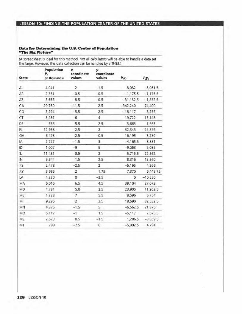
LESSON 10: FINDING THE POPULATION CENTER OF THE UNITED STATES
Data for Determining the U.S. Center of Population "The Big Picture"
(A spreadsheet is ideal for this method. Not all calculators will be able to handle a data set this large. However, this data collection can be handled by a Tl-83.)
Population x- y-P; coordinate coordinate
State (in thousands) values values P;X; P~;
AL 4,041 2 -1.5 8,082 -6,061.5
AR 2,351 -0.5 -0.5 -1,175.5 -1, 175.5
AZ 3,665 -8.5 -0.5 -31,152.5 -1,832.5
CA 29,760 -11.5 2.5 -342,240 74,400
co 3,294 -5.5 2.5 -18, 117 8,235
CT 3,287 6 4 19,722 13,148
DE 666 5.5 2.5 3,663 1,665
FL 12,938 2.5 -2 32,345 -25,876
GA 6,478 2.5 -0.5 16, 195 -3,239
IA 2,777 -1.5 3 -4, 165.5 8,331
ID 1,007 -9 5 -9,063 5,035
IL 11,431 0.5 2 5,715.5 22,862
IN 5,544 1.5 2.5 8,316 13,860
KS 2,478 -2.5 2 -6, 195 4,956
KY 3,685 2 1.75 7,370 6,448.75
LA 4,220 0 -2.5 0 -10,550
MA 6,016 6.5 4.5 39,104 27,072
MD 4,781 5.0 2.5 23,905 11,952.5
ME 1,228 7 5.5 8,596 6,754
Ml 9,295 2 3.5 18,590 32,532.5
MN 4,375 -1.5 5 -6,562.5 21,875
MO 5, 117 -1 1.5 -5,117 7,675.5
MS 2,573 0.5 -1.5 1,286.5 -3,859.5
MT 799 -7.5 6 -5,992.5 4,794
J.J.8 LESSON 10
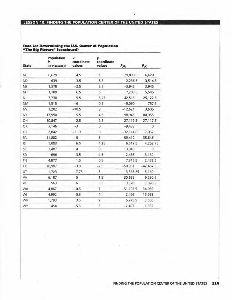
LESSON 10: FINDING THE POPULATION CENTER OF THE UNITED STATES
Data for Determini1111 the U.S. Center of Population "The Bi& Picture" (continued)
Population x- y-P; coordinate coordinate
State (in thousands) values values P;X; P;Y;
NC 6,629 4.5 29,830.5 6,629
ND 639 -3.5 5.5 -2,236.5 3,514.5
NE 1,578 -2.5 2.5 -3,945 3,945
NH 1, 109 6.5 5 7,208.5 5,545
NJ 7,730 5.5 3.25 42,515 25, 122.5
NM 1,515 -6 0.5 -9,090 757 .5
NV 1,202 -10.5 3 -12,621 3,606
NY 17,990 5.5 4.5 98,945 80,955
OH 10,847 2.5 2.5 27,117.5 27,117.5
OK 3,146 -3 0 -9,438 0
OR 2,842 -11.3 6 -32, 114.6 17,052
PA 11,882 5 3 59,410 35,646
RI 1,003 6.5 4.25 6,519.5 4,262.75
SC 3,487 4 0 13,948 0
SD 696 -3.5 4.5 -2,436 3, 132
TN 4,877 1.5 0.5 7,315.5 2,438.5
TX 16,987 -3 .0 -2.5 -50,961 -42,467.5
UT 1,723 -7.75 3 -13,353.25 5, 169
VA 6,187 5 1.5 30,935 9,280.5
VT 563 6 5.5 3,378 3,096.5
WA 4,867 -10.5 7 -51, 103.5 34,069
WI 4,992 0.5 4 2,496 19,968
WV 1,793 3.5 2 6,275.5 3,586
WY 454 -5.5 3 -2,497 1,362
FINDING THE POPULATION CENTER OF THE UNITED STATES 119
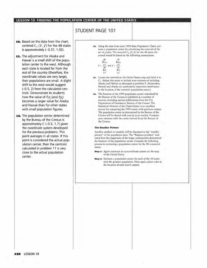
LESSON 10: FINDING THE POPULATION CENTER OF THE UNITED STATES
:10. Based on the data from the chart, centroid C1 (x, fl for the 48 states is approximately (-0.37, 1.92).
n. The adjustment for Alaska and Hawaii is a small shift of the population center to the west. Although each state is located far from the rest of the country (therefore, the coordinate values are very large), their populations are small. A slight shift to the west would suggest (-0.5, 2) from the calculated centroid. Demonstrate to students how the value of P;X; (and f}y;) becomes a larger value for Alaska and Hawaii than for other states with small population figures.
:i:a. The population center determined by the Bureau of the Census is approximately C (-0.5, 1.7) given the coordinate system developed for the previous problems. This point averages in all states. If this point is considered the actual population center, then the centroid calculated in problem 11 is very close to the actual population center.
~zo LESSON 10
STUDENT PAGE 101
10. Using the data from your 1990 State Population Chart, estimate a population center by calculating the centroid of the se.t of points. The. ce.ntroicl \.1 (f, )i) for the. 48 stare..• cliscussed would be based on the following summations:
48 48
LP1 xi l:.Pix1
x = _.!=_!__ and y = _.!=_l_ 48 48
!:P, !:P, i=l i=l
u. Locate the centroid on the United States map and label it as C1. Adjust this point to include your estimate of including Alaska and Hawaii as discussed in problem 9. (Remember, Hawaii and Alaska are particularly important small states in the location of the country's population center.)
u. The location of the 1990 population center calculated by the Bureau of the Census is published in a number of sources, including special publications from the U.S. Department of Commerce, Bureau of the Census. The Statistical Abstract of the United States is an excellent source for comparing the 1990 center with previous centers. The population center as determined by the Bureau of the Census will be shared with you by your teacher. Compare your estimate with the center derived from the Bureau of the Census.
The Smaller Picture
Another method to consider will be discussed as the "smaller picture" of the population data. The "Belgium problem" indicated how the magnitude of the larger communities determined the location of the population center. Consider the following process in estimating a population center for the 48 connected states:
Step :11 Again construct an xy-coordinate system on the map of the United States.
Step :i: Estimate a population center for each of the 10 states with the greatest population. Here again, place a dot at the location of each state's capital.
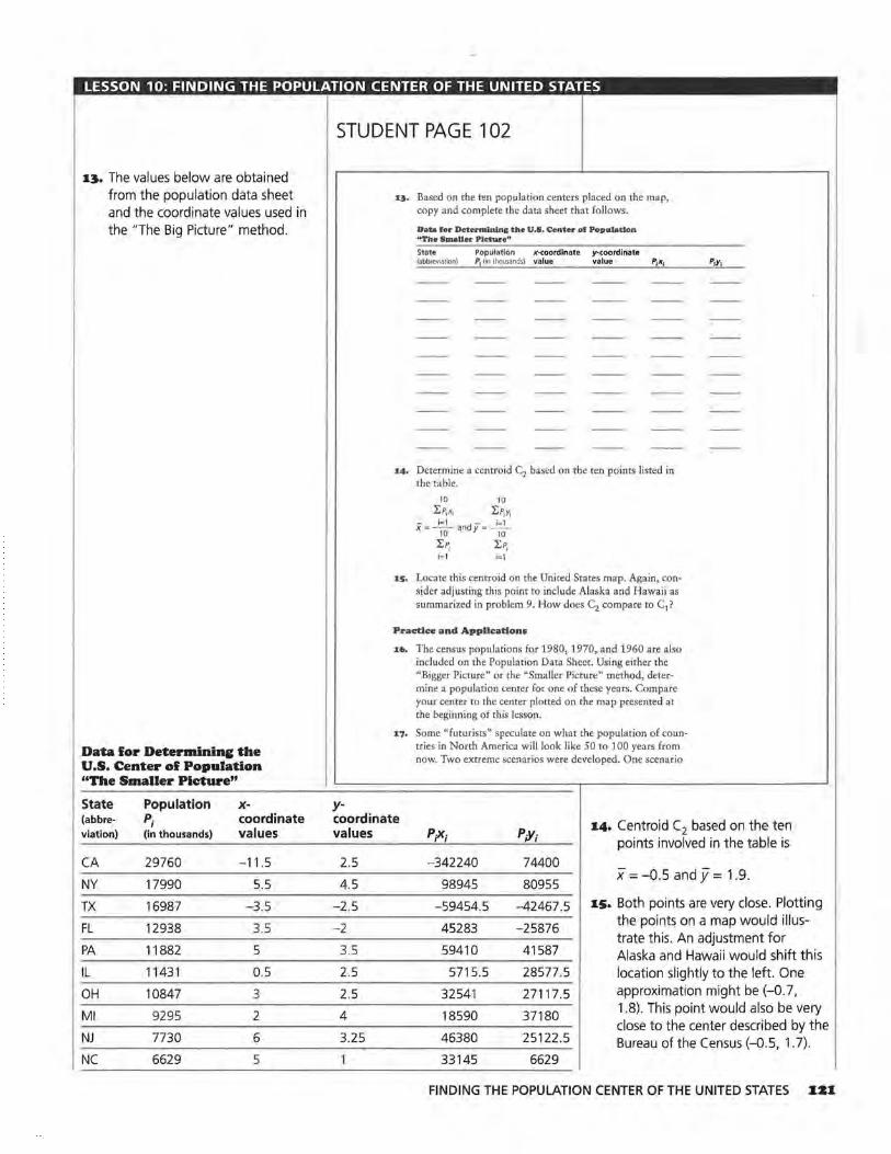
LESSON 10: FINDING THE POPULATION CENTER OF THE UNITED STATES
1::1. The values below are obtained from the population data sheet and the coordinate values used in the "The Big Picture" method.
Data for Determinine the U.S. Center of Population "The Smaller Picture"
State Population x-(abbre- P; coordinate viation) (in thousands) values
CA 29760 -11 .5
NY 17990 5.5
TX 16987 -3.5
FL 12938 3.5
PA 11882 5
IL 11431 0.5
OH 10847 3
Ml 9295 2
NJ 7730 6
NC 6629 5
STUDENT PAGE 102
y-
1~. Based on the ten population centers placed on the map, copy and complete the data sheet that follows.
Data lor Dete.rmintne the U.S. Center ol Populadon "The Smaller Picture"
State Population x-coordlnate y-coordinate (abbreviation) P1 (in thousands) value value Pjxi P1yi
14. Determine a centroid C2 based on the ten points listed in the table.
10 10
L~xi LPiY;
x = .J.=.1._ andy = .J.=.1._ 10 10
LP; LP, i=l i=l
15. Locate this centroid on the United States map. Again, consider adj us ting this point to include Alaska and Hawaii as summarized in problem 9. How does C2 compare to C1?
Practice and Applications
16. The census populations for 1980, 1970, and 1960 are also included on the Population Data Sheet. Using either the "Bigger Picture" or the "Smaller Picture" method, determine a population center for one of these years. Compare your center to the center plotted on the map presented at the beginning of this lesson.
17. Some "futurists" speculate on what the population of countries in North America will look like 50 to 100 years from now. Two extreme scenarios were developed. One scenario
coordinate 1:4. Centroid C2 based on the ten values P;X; P;Y; points involved in the table is
2.5 - 342240 74400
4.5 98945 80955 x = -0.5 and y = 1.9.
-2.5 -59454.5 -42467.5 i:s. Both points are very close. Plotting
-2
3.5
45283 -25876 the points on a map would illus-trate this. An adjustment for
59410 41587 Alaska and Hawaii would shift this 2.5 5715.5 28577.5 location slightly to the left. One
2.5 32541 27117.5 approximation might be (-0.7,
4
3.25
18590 37180 1.8). This point would also be very close to the center described by the
46380 25122.5 Bureau of the Census (-0.5, 1. 7). 1 33145 6629
FINDING THE POPULATION CENTER OF THE UNITED STATES 1Z1
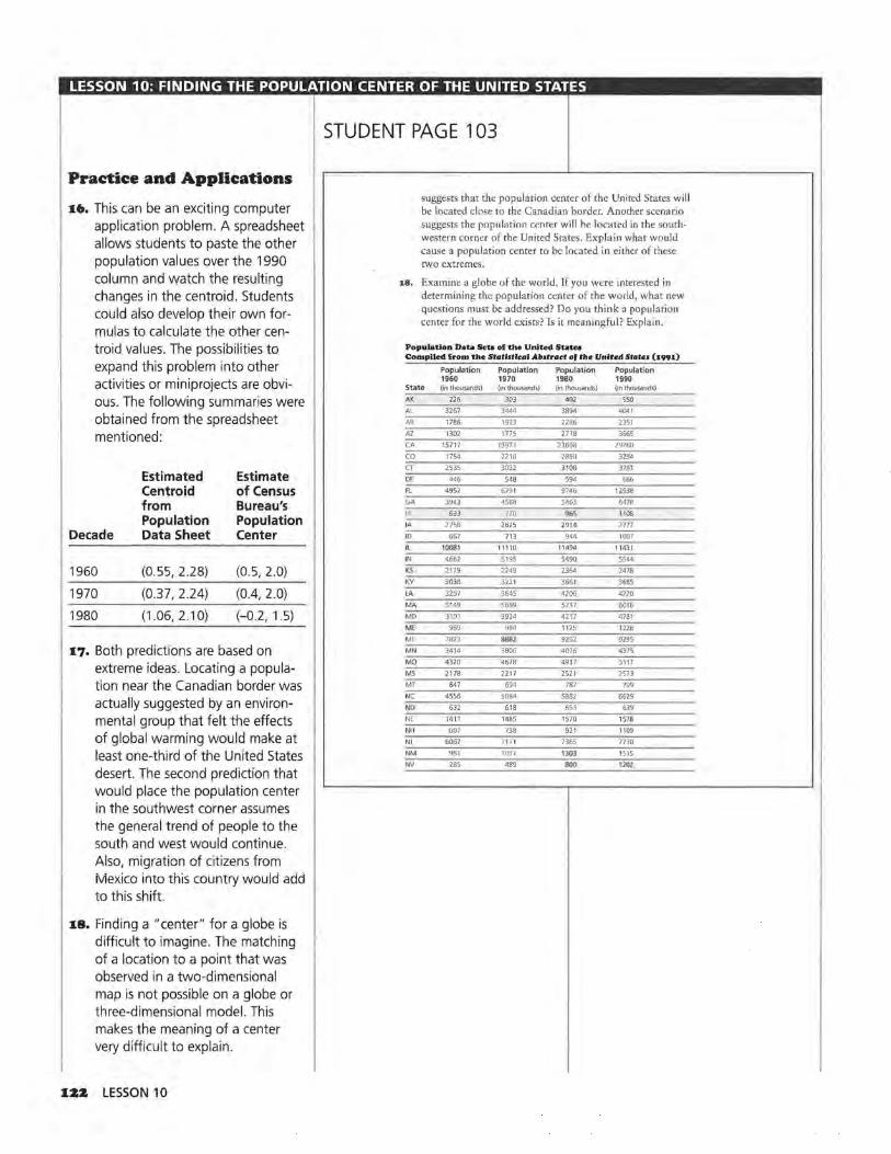
LESSON 10: FINDING THE POPULATION CENTER OF THE UNITED STATES
Practice and Applications
16. This can be an exciting computer application problem . A spreadsheet allows students to paste the other population values over the 1990 column and watch the resulting changes in the centroid. Students could also develop their own formulas to calculate the other centroid values. The possibilities to expand this problem into other activities or miniprojects are obvious. The following summaries were obtained from the spreadsheet mentioned:
Estimated Estimate Centroid of Census from Bureau's Population Population
Decade Data Sheet Center
1960 (0.55, 2.28) (0.5, 2.0)
1970 (0.37, 2.24) (0.4, 2.0)
1980 (1.06, 2.10) (-0.2, 1.5)
17. Both predictions are based on extreme ideas. Locating a population near the Canadian border was actually suggested by an environmental group that felt the effects of global warming would make at least one-third of the United States desert. The second prediction that would place the population center in the southwest corner assumes the general trend of people to the south and west would continue. Also, migration of citizens from Mexico into this country wouid add to this shift.
18. Finding a "center" for a globe is difficult to imagine. The matching of a location to a point that was observed in a two-dimensional map is not possible on a globe or three-dimensional model. This makes the meaning of a center very difficult to explain .
J.22 LESSON 10
STUDENT PAGE 103
suggests that the population center of the United States will be located close to the Canadian border. Another scenario suggests the population cwter will be located in the south-western corner of the United States. Explain what would cause a population center to be located in either of these two extremes.
18. Examine a globe of the world. If you were interested in determining the population center of the world, what new questions must be addressed? Do you think a population center for the world exists? Is it meaningful? Explain.
Population Data Seta ol the United State• Compiled from the Statbtfeal Ab.straet of the United State.s (1"1)
Population Population Population Population 1960 1970 1980 1990
State (in thousands) (in thousands) (in thousands) (in thousands)
AK 226 303 402 550
Al 3267 3444 3894 4041
AR 1786 1923 2286 2351
AZ 1302 1775 2718 3665
CA 15717 19971 23668 29760
co 1754 22 10 2890 3294
CT 2535 3032 3108 3287
DE 446 548 594 666
FL 4952 6791 9746 12938
GA 3943 4588 5463 6478
HI 633 770 965 1108
IA 2758 2825 2914 2777
ID 667 713 944 1007
IL 10081 11110 1149• 11431
IN 4662 5195 5490 5544
~ 2179 2249 2364 2478
KY 3038 322l 3661 3685
LA 3257 3645 4206. 4220
MA 5149 5689 5737 6016
MD 3101 3924 4217 4781
M( 969 994 1125 1228
Ml 7823 888i 9262 9295
MN 3414 3806 4076 4375
MO 4320 4678 4917 5117
MS 2178 2217 2521 2573
MT 647 694 787 799
NC 4556 5084 5882 6629
NP 632 618 653 639
NE 1411 1485 1570 1578
NII G07 738 921 1109
NJ 6067 7171 7365 7730
NM 951 1017 IJOJ 1515
NV 285 489 BOO 1202
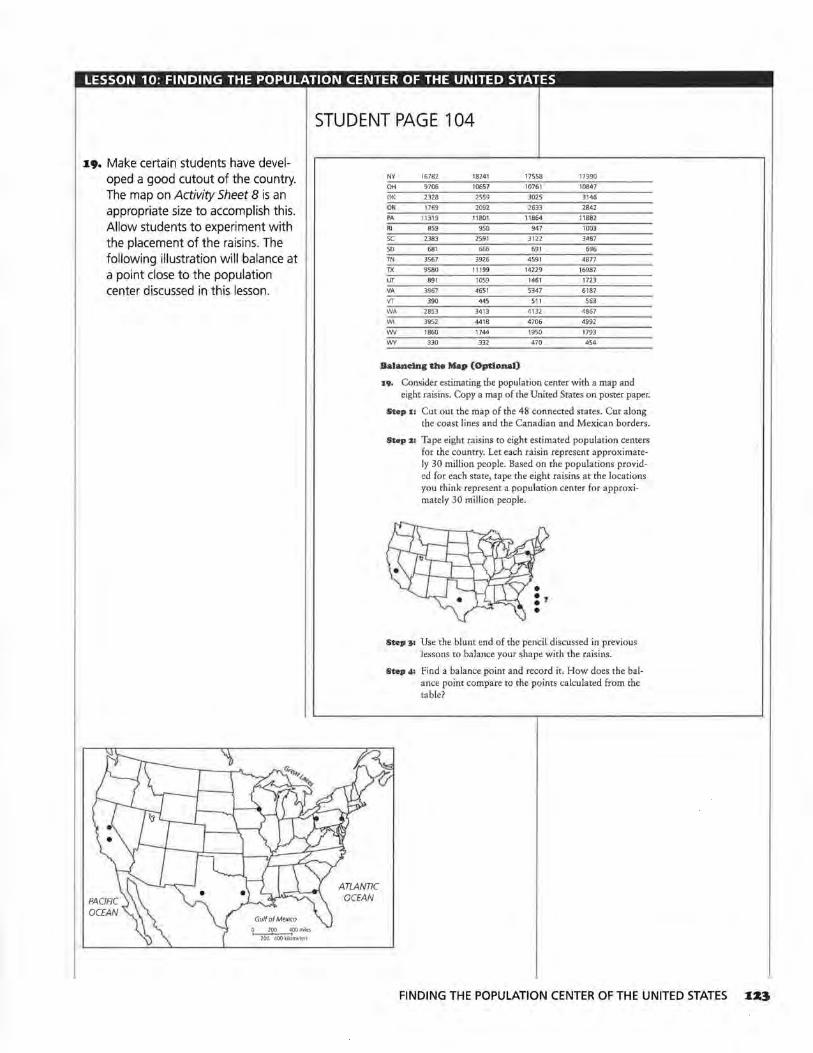
LESSON 10: FINDING THE POPULATION CENTER OF THE UNITED STATES
••· Make certain students have developed a good cutout of the country. The map on Activity Sheet 8 is an appropriate size to accomplish this. Allow students to experiment with the placement of the ra isins. The following illustration will balance at a point close to the population center discussed in this lesson.
O 200 400miles .............-. 200 400 ki lometers
STUDENT PAGE 104
ATLANTIC OCEAN
NY 16782 18241 17558 17990
OH 9706 10657 10761 10847
OK 2318 2559 3025 3146
OR 1769 2092 2633 1842
PA 11319 11801 11864 11881
RI 859 950 947 1003
SC 1383 2591 3122 3487
so 681 666 691 696
TN 3567 3926 4591 4877
TX 9580 111 99 14229 16987
UT 891 1059 1461 1723
VA 3967 4651 5347 6187
VT 390 445 511 563
WA 2853 3413 4132 4867
WI 3952 4418 4706 4992
WV 1860 1744 1950 1793
WY 330 332 470 454
Balancing the Map (Optional)
•9· Consider estimating the population center with a map and eight raisins. Copy a map of the United States on poster paper.
Step u Cut out the map of the 48 connected states. Cut along the coast lines and the Canadian and Mexican borders.
Step :111 Tape eight raisins to eight estimated population centers for the country. Let each raisin represent approximately 30 million people. Based on the populations provided for each state, tape the eight raisins at the locations you think represent a population center for approximately 30 million people.
Step J1 Use the blunt end of the pencil discussed in previous lessons to balance your shape with the raisins.
Step 41 Find a balance point and record it. How does the balance point compare to the points calculated from the table?
FINDING THE POPULATION CENTER OF THE UNITED STATES IZ3

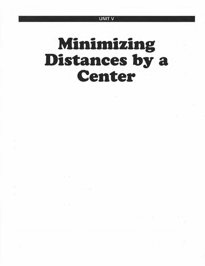
UNIT V
Mini1nizing Distances by a
Center

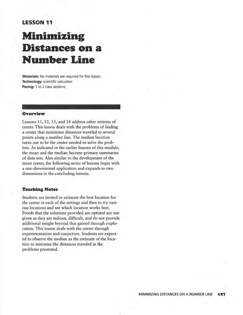
LESSON 11
Mini1nizing Distances on a Nu1nber Line Materials: No materials are required for this lesson. Technology: scientific calculator
Pacing: 1 to 2 class sessions
Overview
Lessons 11, 12, 13, and 14 address other notions of center. This lesson deals with the problems of finding a center that minimizes distances traveled to several points along a number line. The median location turns out to be the center needed to solve the problem. As indicated in the earlier lessons of this module, the mean and the median become primary summaries of data sets. Also similar to the development of the mean center, the following series of lessons begin with a one-dimensional application and expands to two dimensions in the concluding lessons.
Teaching Notes
Students are invited to estimate the best location for the center in each of the settings and then to try various locations and see which location works best. Proofs that the solutions provided are optimal are not given as they are tedious, difficult, and do not provide additional insight beyond that gained through exploration. This lesson deals with the center through experimentation and conjecture. Students are expected to observe the median as the estimate of the location to minimize the distances traveled in the problems presented.
MINIMIZING DISTANCES ON A NUMBER LINE IZ7
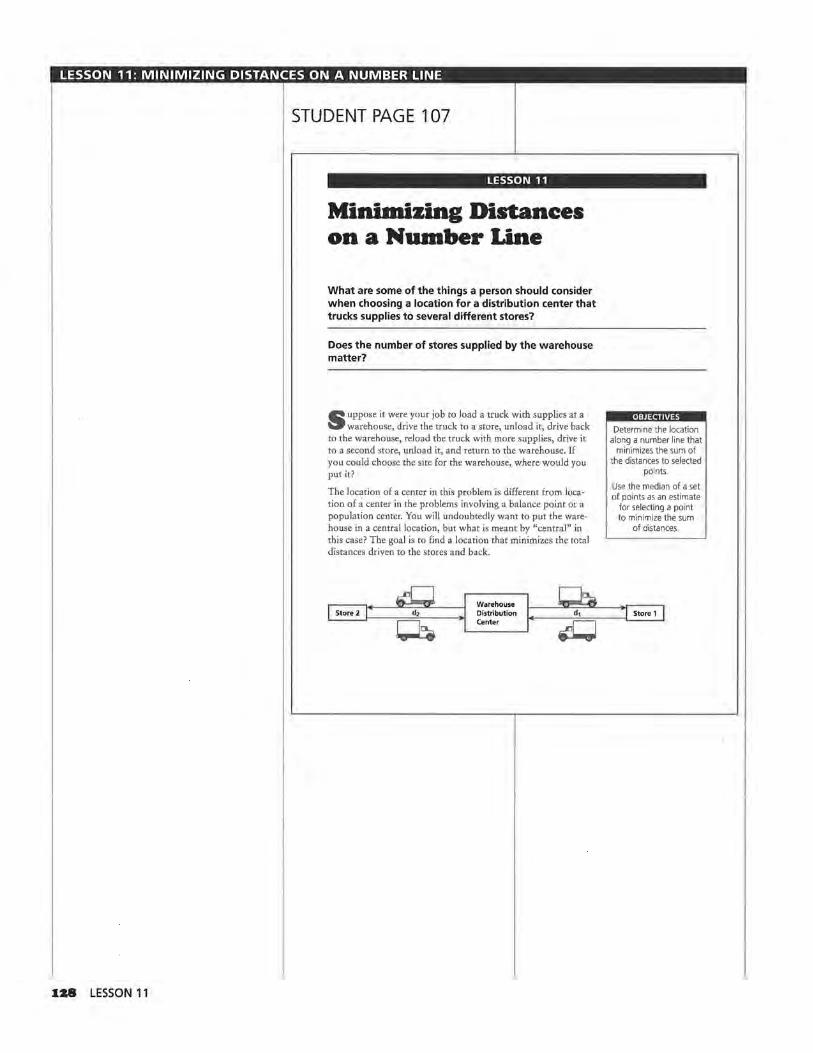
LESSON 11: MINIMIZING DISTANCES ON A NUMBER LINE
J.Z8 LESSON 11
STUDENT PAGE 107
LESSON 11
Minimizing Distances on a Number Line
What are some of the things a person should consider when choosing a location for a distribution center that trucks supplies to several different stores?
Does the number of stores supplied by the warehouse matter?
S up pose it were your job to load a truck with supplies at a warehouse, drive the truck to a store, unload it, drive back
to the warehouse, reload the truck with more supplies, drive it to a second store, unload it, and return to the warehouse. If you could choose the site for the warehouse, where would you put it?
The location of a center in this problem is different from location of~ center in the problems involving a balance point or a population center. You will undoubtedly want to put the warehouse in a central location, but what is meant by "central" in this case? The goal is to find a location that minimizes the total distances driven to the stores and back.
Warehouse Distribution Center
. : Determine the location
along a number line that minimizes the sum of
the distances to selected points
Use the median of a set of points as an estimate
for selecting a point to minimize the sum
of distances.
Store 1
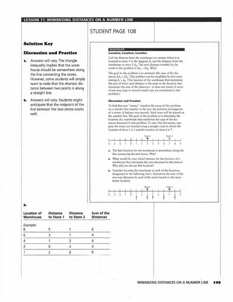
LESSON 11: MINIMIZING DISTANCES ON A NUMBER LINE
Solution Key
Discussion and Practice
1.. Answers will vary. The triangle inequality implies that the warehouse should be somewhere along the line connecting the stores. However, some students will simply want to note that the shortest distance between two points is along a straight line.
z. Answers will vary. Students might anticipate that the midpoint of the line between the two stores works well.
~.
Location of Distance Distance Warehouse to Store 1 to Store 2
Example: 8 5
6 3
4 3
3 0 4
2 6
STUDENT PAGE 108
INVESTIGATE
Location, Location, Location
Call the distance from the warehouse (no matter where it is located) to store 1 in the diagram d 1 and the distance from the warehouse to store 2 d2. The total distance traveled by the truck in this problem is 2d1 + 2d2. Why?
The goal in this problem is to minimize this sum of the distances 2d1 + 2d2• This problem can be simplified by first minimizing d1 + d2. (The location of the warehouse that minimizes the sum of twice each distance is the same as the location that minimizes the sum of the distances-it does not matter if several one-way trips or several round trips are considered in this problem.)
Discussion and Practice
To find this new "center," visualize the setup of this problem on a number line (similar to the way the previous investigation of a center of balance was started). Each store will be placed on the number line. The goal of the problem is to determine the location of a warehouse that minimizes the sum of the distances discussed in this problem. To start this discussion, suppose the stores are located along a straight road in which the location of store 1 is 3 and the location of store 2 is 7.
Store I Store 2
T T - 4 -3 -2 - 1 0
1. The best location for the warehouse is somewhere along the line connecting the two stores. Why?
2. What would be your initial estimate for the location of a warehouse that minimizes the sum discussed in this lesson? Why did you choose that location?
:t. Consider locating the warehouse at each of the locations designated in the following chart. Determine the sum of the one-way distances to each of the stores based on the warehouse location:
Store 1 Store 2
I I T I I T I -4 -3 -2 -1 0 1 3 4 6 7 8
t t t t t
Sum of the Distances
6
4
4
4
8
MINIMIZING DISTANCES ON A NUMBER LINE IZ9
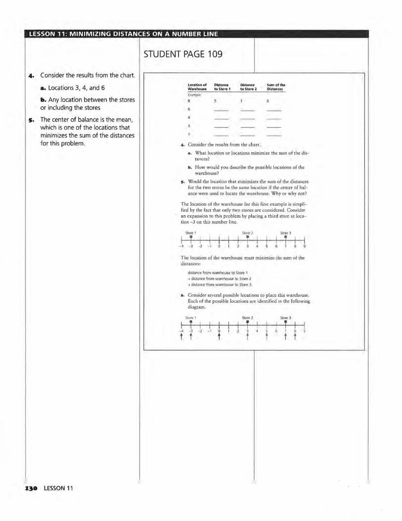
LESSON 11: MINIMIZING DISTANCES ON A NUMBER LINE
4. Consider the results from the chart.
a. Locations 3, 4, and 6
b. Any location between the stores or including the stores
5. The center of balance is the mean, which is one of the locations that minimizes the sum of the distances for this problem.
~~O LESSON 11
STUDENT PAGE 109
location of Distance Warehouse to Store 1
Example:
8
6
s
Distance to Store 2
4, Consider the results from the chart.
Sum of the Distances
a. What location or locations minimize the sum of the distances?
II. How would you describe the possible locations of the warehouse?
5. Would the location that minimizes the sum of the distances for the two stores be the same location if the center of balance were used to locate the warehouse. Why or why not?
The location of the warehouse for this first example is simplified by the fact that only two stores are considered. Consider an expansion to this problem by placing a third store at location -3 on this number line.
Store 1 Store 2 Store 3
T I T T -4 -3 -2 -1
The location of the warehouse must minimize the sum of the distances:
distance from warehouse ta Store 1
+ distance from warehouse to Store 2
+ distance from warehouse to Store 3.
6. Consider several possible locations to place this warehouse. Each of the possible locations are identified in the following diagram.
Store 1 Store 2 Store 3
I T I T I T I -4 -3 -2 _, 0 3 4 5 7 8
t t t t t t t
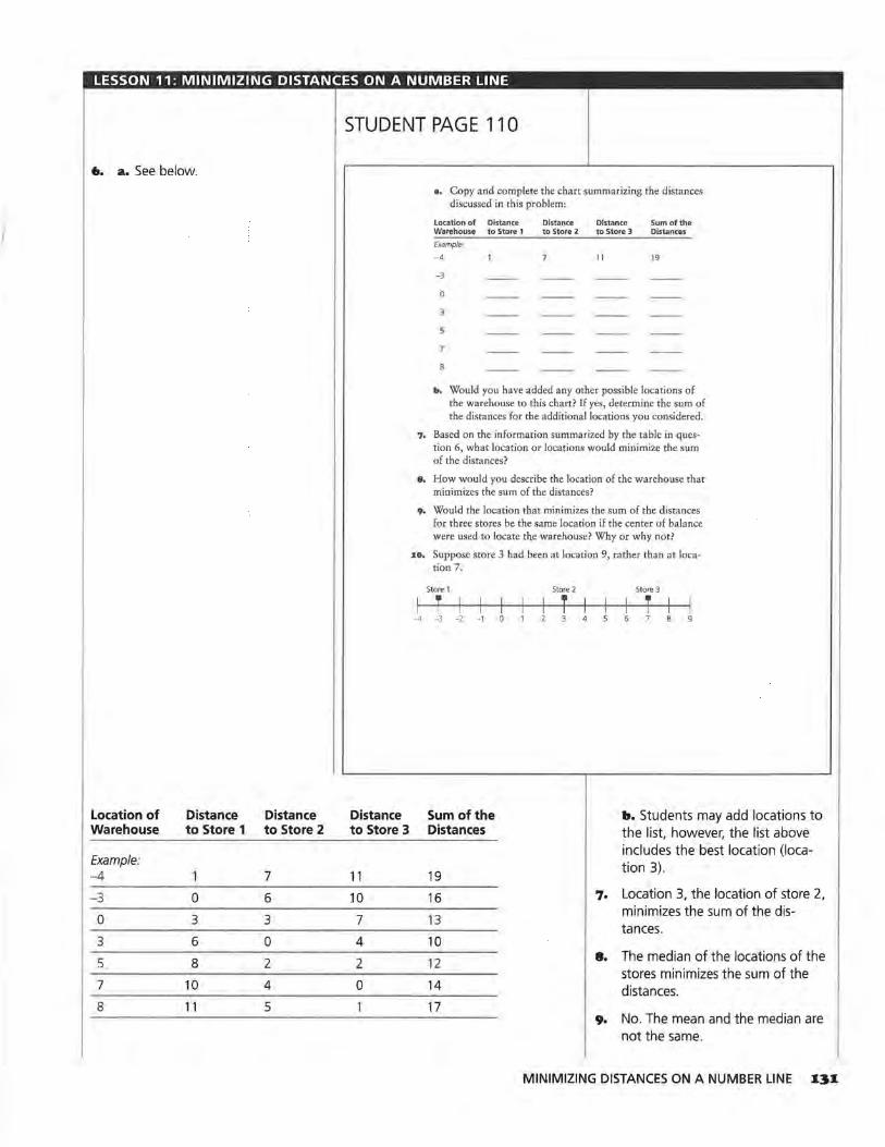
LESSON 11: MINIMIZING DISTANCES ON A NUMBER LINE
6. a. See below.
Location of Distance Distance Warehouse to Store 1 to Store 2
Example: -4 7
-3 0 6
0 3 3
3 6 0
5 8 2
7 10 4
8 11 5
STUDENT PAGE 110
Distance to Store 3
11
JO
7
4
2
0
a. Copy and complete the chart summarizing the distances discussed in this problem:
location of Distance Distance Distance Sum of the Warehouse to Store 1 to Store 2 to Store 3 Distances Example,
-4 I 11 19
-3
b. Would you have added any other possible locations of the warehouse to this chart? If yes, determine the sum of the distances for the additional locations you considered.
7. Based on the information summarized by the table in question 6, what location or locations would minimize the sum of the distances?
8. How would you describe the location of the warehouse that minimizes the sum of the distances?
9, Would the location that minimizes the sum of the distances for three stores be the same location if the center of balance were used to locate the warehouse? Why or why not?
10. Suppose store 3 had been at location 9, rather than at location 7.
Store 1 Store 2 Store 3
T T I T -4 -3 -2 - 1 3 4
Sum of the b. Students may add locations to Distances the list, however, the list above
includes the best location (loca-
19 tion 3).
16 7. Location 3, the location of store 2,
13 minimizes the sum of the dis-tances.
10
12 8. The median of the locations of the stores minimizes the sum of the
14 distances. 17
9. No. The mean and the median are not the same.
MINIMIZING DISTANCES ON A NUMBER LINE 131
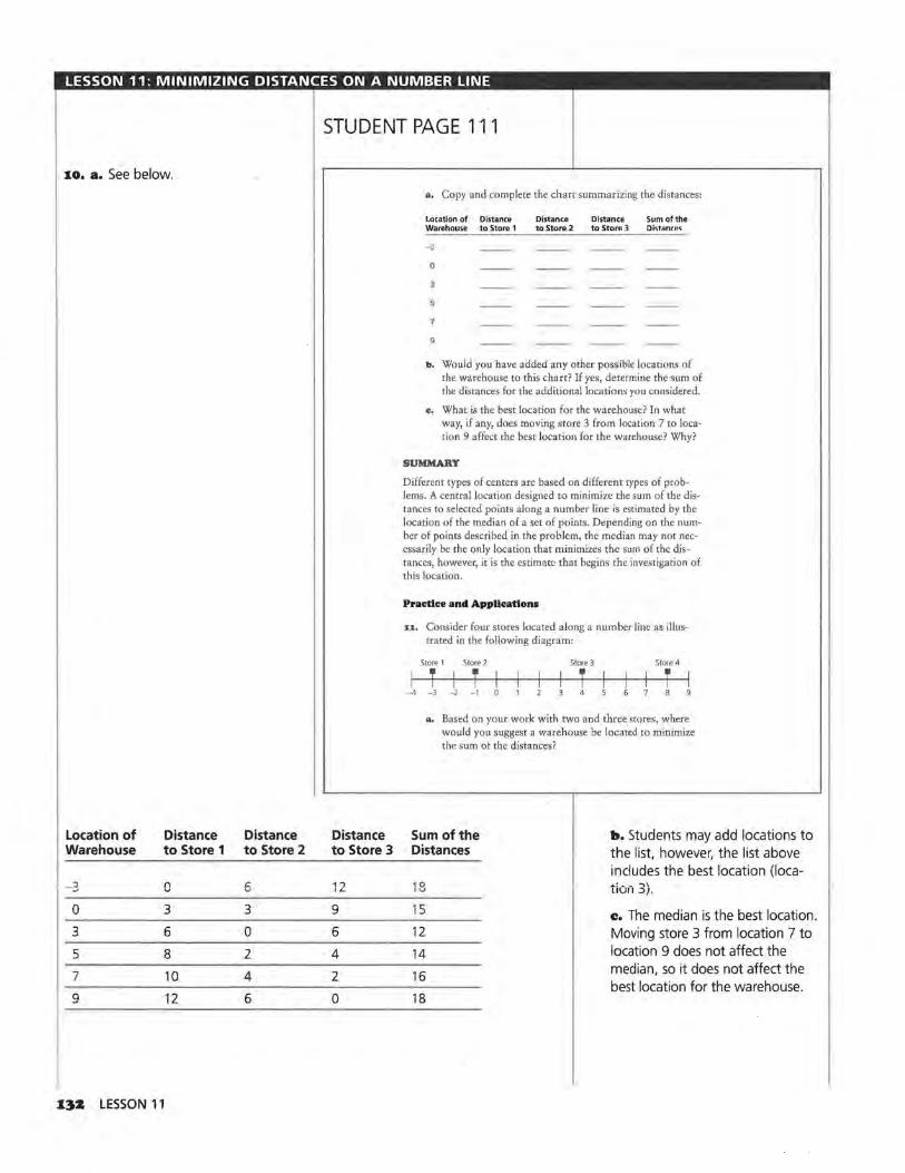
LESSON 11: MINIMIZING DISTANCES ON A NUMBER LINE
xo. a. See below.
Location of Distance Distance Warehouse to Store 1 to Store 2
-3 0 6
0 3 3
3 6 0
5 8 2
7 10 4
9 12 6
x~z LESSON 11
STUDENT PAGE 111
Distance to Store 3
12
9
6
4
2
0
a. Copy and complete the chart summarizing the distances:
Location of Distance Warehouse to Store 1
-3
0
Distance Distance Sum of the to Store 2 to Ston1 3 Di"itanrP.c;
b. Would you have added any other possible locations of the warehouse to this chart? If yes, determine the sum of the distances for the additional locations you considered.
c. What is the best location for the warehouse? In what way, if any, does moving store 3 from location 7 to location 9 affect the best location for the warehouse? Why?
SUMMARY
Different types of centers are based on different types of problems. A central location designed to minimize the sum of the distances to selected points along a number line is estimated by the location of the median of a set of points. Depending on the number of points described in the problem, the median may not necessarily be the only location that minimizes the sum of the distances, however, it is the estimate that begins the investigation of this location.
Practice and Applications
:u. Consider four stores located along a number line as illustrated in the following diagram:
Store 1 Store 2 Store 3 Store 4
T I T T T -4 -3 -2 -1
a. Based on your work with two and three stores, where would you suggest a warehouse be located to minimize the sum of the distances?
Sum of the b. Students may add locations to Distances the list, however, the list above
includes the best location (loca-10 . : _ - ""'\\ IU LtUll :::>) .
15 c. The median is the best location. 12 Moving store 3 from location 7 to
14 location 9 does not affect the
16 median, so it does not affect the best location for the warehouse.
18
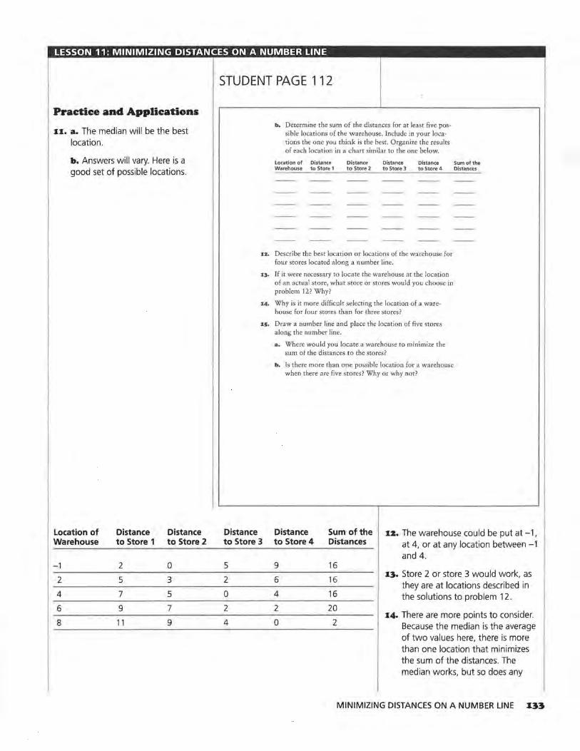
LESSON 11 : MINIMIZING DISTANCES ON A NUMBER LINE
Practice and Applications
1.1.. a. The median will be the best location.
b. Answers will vary. Here is a good set of possible locations.
Location of Distance Distance Warehouse to Store 1 to Store 2
-1 2 0
2 5 3
4 7 5
6 9 7
8 11 9
STUDENT PAGE 112
Distance
b. Determine the sum of the distances for at least five possible locations of the warehouse. Include in your locations the one you think is the best. Organize the results of each location in a chart similar to the one below.
Location of Distance Distance Distance Distance Sum of the Warehouse to Store 1 to Store 2 to Store 3 to Store 4 Distances
1z. Describe the best location or locations of the warehouse for four stores located along a number line.
1.1. If it were necessary to locate the warehouse at the location of an actual store, what store or stores would you choose in problem 12? Why?
14. Why is it more difficult selecting the location of a warehouse for four stores than for three stores?
1s. Draw a number line and place the location of five stores along the number line.
a. Where would you locate a warehouse to minimize the sum of the distances to the stores?
b. Is there more than one possible location for a warehouse when there are five stores? Why or why not?
Distance Sum of the 1.z. The warehouse could be put at -1, to Store 3 to Store 4 Distances at 4, or at any location between -1
and 4. 5 9 16
2 6 16 1.~. Store 2 or store 3 would work, as
they are at locations described in 0 4 16 the solutions to problem 12. 2 2 20
1.4. There are more points to consider. 4 0 2 Because the median is the average
of two values here, there is more than one location that minimizes the sum of the distances. The median works, but so does any
MINIMIZING DISTANCES ON A NUMBER LINE 133
LESSON 11 : MINIMIZING DISTANCES ON A NUMBER LINE
location between the two stores used to calculate the median.
f s. a. Answers will vary. In each case,
however, the median will be the · best location for the warehouse.
b. No. Since 5 is an odd number, the median is the same as the location of one of the stores and provides the unique solution.
I34 LESSON 11
LESSON 12
Taxicab Geo1netry Materials: Activity Sheet 13 Technology: scientific calculator Pacing: 1 to 2 class sessions
Overview
This lesson expands the description of the problem started in Lesson 11 to a two-dimensional appli<::a-
. tion. The problems posed to the student require a minimization of the distances traveled to several locations on a grid. The distances are measured in units representing only up/down or left/right units (i.e., taxicab units). Locations are conjectured and then tested. From the work in Lesson 11, students are expected to estimate the requested centers by using the median values of the locations. This median center must be determined using both the x- and y-locations of the warehouses discussed in the problems. The median location provides the desired minimization of traveled distances and suggests to the students a generalization of this investigation.
Teaching Notes
Charts are carefully organized to encourage students to investigate a location and record the resulting distances. The organization of the charts was designed to guide the students into expanding the conclusions derived from the previous lesson. The lesson ends with students seeing a weighted value to one of the warehouse locations. The weighted value represents a location of a warehouse that is traveled to more than once. The difference between the interpretation of a weighted location in this lesson is contrasted to the weighted value of a location in the mean center applications.
TAXICAB GEOMETRY 1:JS
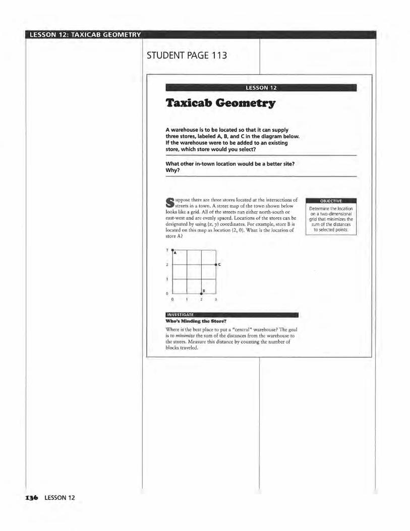
LESSON 12: TAXICAB GEOMETRY
136 LESSON 12
STUDENT PAGE 113
LESSON 12
Taxieab Geometry
A warehouse is to be located so that it can supply three stores, labeled A, B, and C in the diagram below. If the warehouse were to be added to an existing store, which store would you select?
What other in-town location would be a better site? Why?
S uppose there are three stores located at the intersections of streets in a town. A street map of the town shown below
looks like a grid. All of the streets run either north-south or east-west and are evenly spaced. Locations of the stores can be designated by using (x, y) coordinates. For example, store B is located on this map as location (2, 0). What is the location of store A?
A
8
0
INVESTIGATE
Who's Minding the Store?
Where is the best place to put a "central" warehouse? The goal is to minimize the sum of the distances from the warehouse to the stores. Measure this distance by counting the number of blocks traveled.
Determine the location on a two-dimensional
grid that minimizes the sum of the distances to selected points
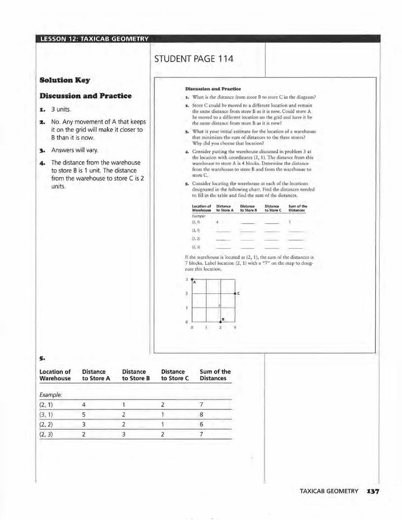
LESSON 12: TAXICAB GEOMETRY
Solution Key
Discussion and Practice
x. 3 units.
z. No. Any movement of A that keeps it on the grid will make it closer to B than it is now.
3. Answers will vary.
4. The distance from the warehouse to store B is 1 unit. The distance from the warehouse to store C is 2 units.
s.
Location of Distance Distance Warehouse to Store A to Store B
Example:
(2, 1) 4
(3, 1) 5 2
(2, 2) 3 2
(2, 3) 2 3
STUDENT PAGE 114
Distance
Discussion and Praetiee
1. What is the distance from store B to store C in the diagram?
z. Store C could be moved to a different location and remain the same distance from store B as it is now. Could store A be moved to a different location on the grid and have it be the same distance from store B as it is now?
~. What is your initial estimate for the location of a warehouse that minimizes the sum of distances to the three stores? Why did you choose that location?
4, Consider putting the warehouse discussed in problem 3 at the location with coordinates (2, 1 ). The distance from this warehouse to store A is 4 blocks. Determine the distance from the warehouse to store B and from the warehouse to store C.
5, Consider locating the warehouse at each of the locations designated in the following chart. Find the distances needed to fill in the table and find the sum of the distances.
Location of Distance Distance Distance Sum of the Warehouse to Store A to Store B to Store C Distances
Example:
(2, 1) 4
(3, 1)
(2, 2)
(2, 3)
If the warehouse is located at (2, 1 ), the sum of the distances is 7 blocks. Label location (2, 1) with a "7" on the map to designate this location.
3 A
2 ------+----+--- c
7
0 0
Sum of the to Store C Distances
2 7
8
6
2 7
TAXICAB GEOMETRY I37
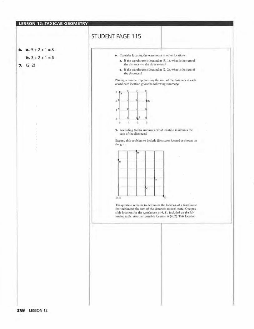
LESSON 12: TAXICAB GEOMETRY
•· a.5+2+1=8
b.3+2+1=6
7. (2, 2)
138 LESSON 12
STUDENT PAGE 115
"· Consider locating the warehouse at other locations.
a. If the warehouse is located at (3, 1), what is the sum of the distances to the three stores?
b. If the warehouse is located at (2, 2), what is the sum of the distances?
Placing a number representing the sum of the distances at each coordinate location gives the following summary:
8 A
2 ! 5 7 c
1 9 ~ ____l_____J
g a e s
0 2 3
7. According to this summary, what location minimizes the sum of the distances?
Expand this problem to include five stores located as shown on the grid.
A
D
c
(0, O)
The question remains to determine the location of a warehouse that minimizes the sum of the distances to each store. One possible location for the warehouse is (4, 1), included on the following table. Another possible location is ( 4, 2). This location
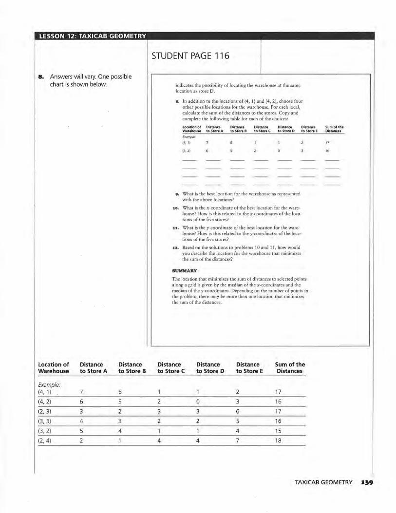
LESSON 12: TAXICAB GEOMETRY
8. Answers will vary. One possible chart is shown below.
Location of Distance Distance Warehouse to Store A to Store B
Example: (4, 1) 7 6
(4, 2) 6 5
(2, 3) 3 2
(3, 3) 4 3
(3, 2) 5 4
(2, 4) 2
STUDENT PAGE 116
indicates the possibility of locating the warehouse at the same location as store D.
8. In addition to the locations of (4, 1) and (4, 2), choose four other possible locations for the warehouse. For each local, calculate the sum of the distances to the stores. Copy and complete the following table for each of the choices:
Location of Distance Distance Distance Distance Warehouse to Store A to Store B to Store C to Store D
Example:
(4, 1) 6
(4, 2) 6 ~
9. What is the best location for the warehouse as represented with the above locations?
Distance to Store E
:10. What is the x-coordinate of the best location for the warehouse? How is this related to the x-coordinates of the locations of the five stores?
u. What is they-coordinate of the best location for the warehouse? How is this related to they-coordinates of the locations of the five stores?
u. Based on the solutions to problems 10 and 11, how would you describe the location for the warehouse that minimizes the sum of the distances?
SUMMARY
The location that minimizes the sum of distances to selected points along a grid is given by the median of the x-coordinates and the median of they-coordinates. Depending on the number of points in the problem, there may be more than one location that minimizes the sum of the distances.
Distance Distance Distance Sum of the to Store C to Store D to Store E Distances
1 1 2 17
2 0 3 16
3 3 6 17
2 2 5 16
1 1 4 15
4 4 7 18
Sum of the Distances
17
16
TAXICAB GEOMETRY
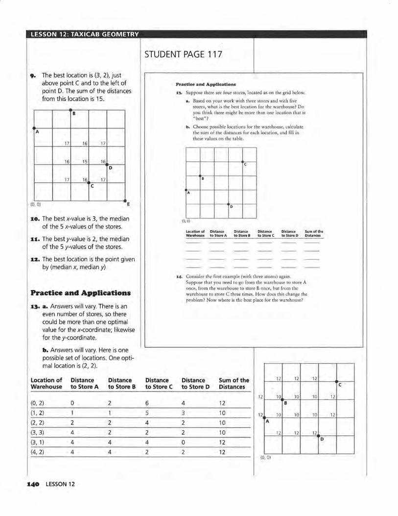
LESSON 12: TAXICAB GEOMETRY
9. The best location is (3, 2), just above point C and to the left of point D. The sum of the distances from this location is 15.
B
A
17 16 17
16 15 16 D
17 16 17 c
(0, 0) E
IO. The best x-value is 3, the median of the 5 x-values of the stores.
u. The best y-value is 2, the median of the 5 y-values of the stores.
I:&. The best location is the point given by (median x, median y)
Practice and Applications
I~. a. Answers will vary. There is an even number of stores, so there could be more than one optimal value for the x-coordinate; likewise for they-coordinate.
b. Answers will vary. Here is one possible set of locations. One optimal location is (2, 2).
Location of Warehouse
(O, 2)
(1, 2)
(2, 2)
(3, 3)
(3 , 1)
(4, 2)
Distance to Store A
0
1
2
4
4
4
1.40 LESSON 12
Distance to Store B
2
1
2
2
4
4
STUDENT PAGE 117
Distance to Store C
6
5
4
2
4
2
Practice and Applications
:13. Suppose there are four stores, located as on the grid below.
a. Based on your work with three stores and with five stores, what is the best location for the warehouse? Do you think there might be more than one location that is "best"?
b. Choose possible locations for the warehouse, calculate the sum of the distances for each location, and fill in these values on the table.
c
A
D
(0,0)
Location of Distance Distance Distance Distance Sum of the Warehouse to Store A to Store B to Store C to Store D Distances
14, Consider the first example (with three stores) again. Suppose that you need to go from the warehouse to store A once, from the warehouse to store B once, but from the warehouse to store C three times. How does this change the problem? Now where is the best place for the warehouse?
Distance Sum of the 12 12
to Store D Distances
12 10 10 4 12 B
3 10 12 10 10
2 10 A
2 10 12 12
0 12
2 12 (0, 0)
12
10
10
12 D
c
12
12
LESSON 12: TAXICAB GEOMETRY
1.4. We can think of this as a problem with five points, where the location of C is the location of three of the five points. The best location for the warehouse is at (median of x, median of y). The median of the five x-coordinates is the x-coordinate of point C, which is 3, and the median of the five y-coordinates is they-coordinate of point C, which is 2. Thus, (3, 2) is the solution. This is like having 5 stores. The best location is (median x, median y), which is (3, 2), the location of store C.
TAXICAB GEOMETRY I4I
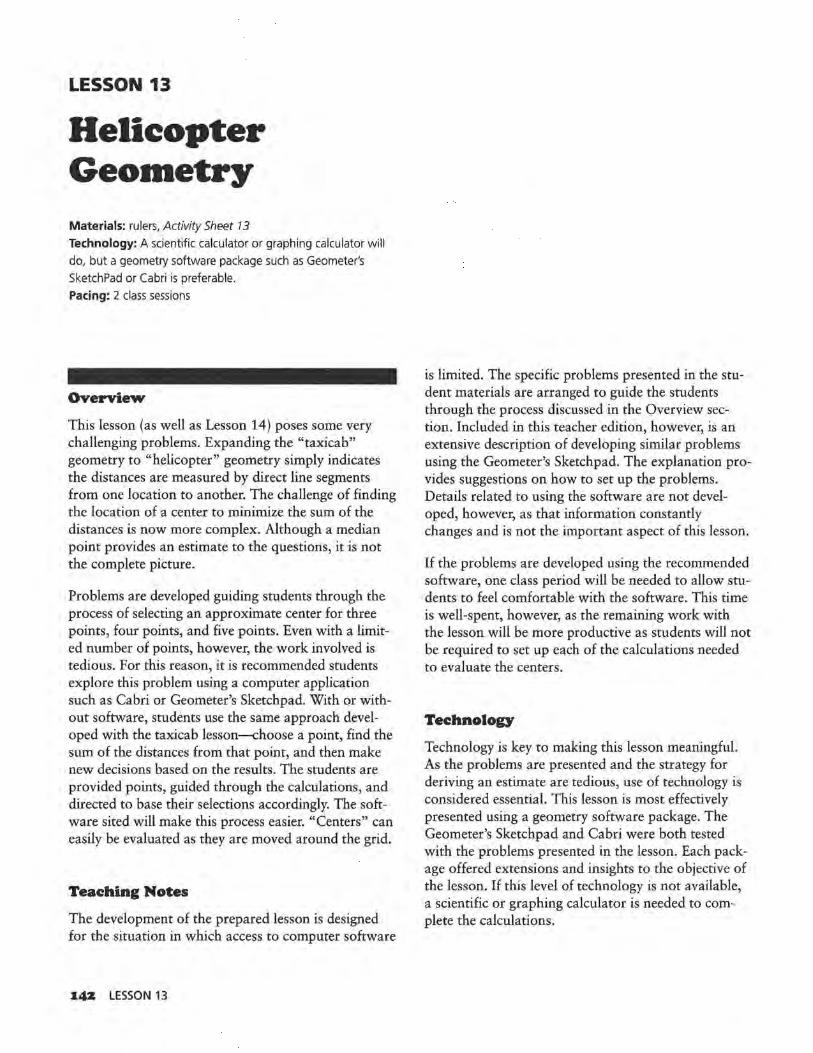
LESSON 13
Helicopter Geo1netry Materials: rulers, Activity Sheet 13
Technology: A scientific calculator or graphing calculator will
do, but a geometry software package such as Geometer's SketchPad or Cabri is preferable.
Pacing: 2 class sessions
Overview
This lesson (as well as Lesson 14) poses some very challenging problems. Expanding the "taxicab" geometry to "helicopter" geometry simply indicates the distances are measured by direct line segments from one location to another. The challenge of finding the location of a center to minimize the sum of the distances is now more complex. Although a median point provides an estimate to the questions, it is not the complete picture.
Problems are developed guiding students through the process of selecting an approximate center for three points, four points, and five points. Even with a limited number of points, however, the work involved is tedious. For this reason, it is recommended students explore this problem using a computer application such as Cabri or Geometer's Sketchpad. With or without software, students use the same approach developed with the taxicab lesson-choose a point, find the sum of the distances from that point, and then make new decisions based on the results. The students are provided points, guided through the calculations, and directed to base their selections accordingly. The software sited will make this process easier. "Centers" can easily be evaluated as they are moved around the grid.
Teaching Notes
The development of the prepared lesson is designed for the situation in which access to computer software
14Z LESSON 13
is limited. The specific problems presented in the student materials are arranged to guide the students through the process discussed in the Overview section. Included in this teacher edition, however, is an extensive description of developing similar problems using the Geometer's Sketchpad. The explanation provides suggestions on how to set up the problems. Details related to using the software are not developed, however, as that information constantly changes and is not the important aspect of this lesson.
If the problems are developed using the recommended software, one class period will be needed to allow students to feel comfortable with the software. This time is well-spent, however, as the remaining work with the lesson will be more productive as students will not be required to set up each of the calculations needed to evaluate the centers.
Technology
Technology is key to making this lesson meaningful. As the problems are presented and the strategy for deriving an estimate are tedious, use of technology is considered essential. This lesson is most effectively presented using a geometry software package. The Geometer's Sketchpad and Cabri were both tested with the problems presented in the lesson. Each package offered extensions and insights to the objective of the lesson. If this level of technology is not available, a scientific or graphing calculator is needed to complete the calculations.
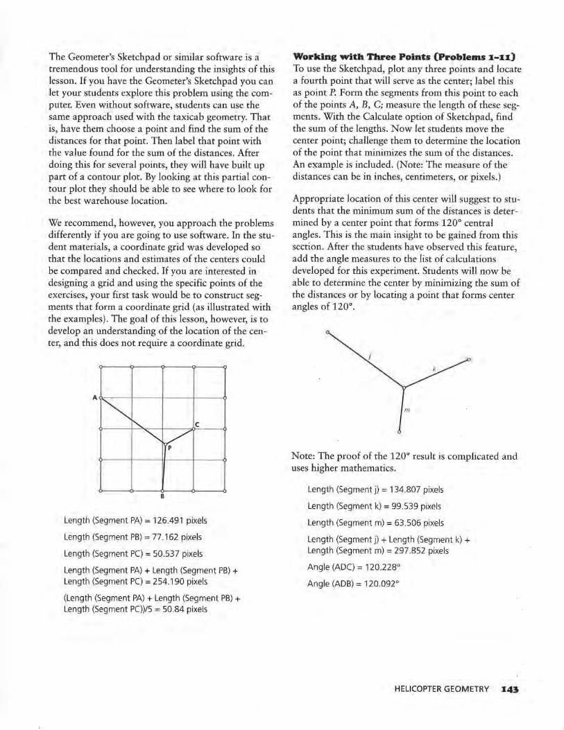
The Geometer's Sketchpad or similar software is a tremendous tool for understanding the insights of this lesson. If you have the Geometer's Sketchpad you can let your students explore this problem using the computer. Even without software, students can use the same approach used with the taxicab geometry. That is, have them choose a point and find the sum of the distances for that point. Then label that point with the value found for the sum of the distances. After doing this for several points, they will have built up part of a contour plot. By looking at this partial contour plot they should be able to see where to look for the best warehouse location.
We recommend, however, you approach the problems differently if you are going to use software. In the student materials, a coordinate grid was developed so that the locations and estimates of the centers could be compared and checked. If you are interested in designing a grid and using the specific points of the exercises, your first task would be to construct segments that form a coordinate grid (as illustrated with the examples). The goal of this lesson, however, is to develop an understanding of the location of the center, and this does not require a coordinate grid.
A
~ "-... c
~ < B
Length (Segment PA) = 126.491 pixels
Length (Segment PB) = 77 .162 pixels
Length (Segment PC) = 50.537 pixels
Length (Segment PA) + Length (Segment PB) + Length (Segment PC) = 254.190 pixels
(Length (Segment PA) + Length (Segment PB) + Length (Segment PC))/5 = 50.84 pixels
Working with Three Points (Problems I-II) To use the Sketchpad, plot any three points and locate a fourth point that will serve as the center; label this as point P. Form the segments from this point to each of the points A, B, C; measure the length of these segments. With the Calculate option of Sketchpad, find the sum of the lengths. Now let students move the center point; challenge them to determine the location of the point that minimizes the sum of the distances. An example is included. (Note: The measure of the distances can be in inches, centimeters, or pixels.)
Appropriate location of this center will suggest to students that the minimum sum of the distances is determined by a center point that forms 120° central angles. This is the main insight to be gained from this section. After the students have observed this feature, add the angle measures to the list of calculations developed for this experiment. Students will now be able to determine the center by minimizing the sum of the distances or by locating a point that forms center angles of 120°.
I
m
Note: The proof of the 120° result is complicated and uses higher mathematics.
Length (Segment j) = 134.807 pixels
Length (Segment k) = 99.539 pixels
Length (Segment m) = 63.506 pixels
Length (Segment j) + Length (Segment k) + Length (Segment m) = 297.852 pixels
Angle (ADC) = 120.228°
Angle (ADB) = 120.092°
HELICOPTER GEOMETRY I43
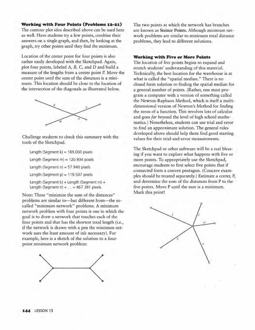
Working with Four Points (Problems IZ-ZI) The contour plot idea described above can be used here as well. Have students try a few points, combine their answers on a single graph, and then, by looking at the graph, try other points until they find the minimum.
Location of the center point for four points is also rather easily developed with the Sketchpad. Again, plot four points, labeled A, B, C, and D and build a measure of the lengths from a center point P. Move the center point until the sum of the distances is a minimum. This location should be close to the location of the intersection of the diagonals as illustrated below.
· Challenge students to check this summary with the tools of the Sketchpad.
Length (Segment k) = 169.000 pixels
Length (Segment m) = 120.934 pixels
Length (Segment n) = 57 .940 pixels
Length (Segment p) = 119.507 pixels
Length (Segment k) + Length (Segment m) + Length (Segment n) + .. . = 467 .381 pixels
Note: These "minimize the sum of the distances" problems are similar to-but different from-the socalled "minimum network" problems. A minimum network problem with four points is one in which the goal is to draw a network that touches each of the four points and that has the shortest total length (i.e., if the network is drawn with a pen the minimum network uses the least amount of ink necessary). For example, here is a sketch of the solution to a fourpoint minimum network problem:
144 LESSON 13
The two points at which the network has branches are known as Steiner Points. Although minimum network problems are similar to minimum total distance problems, they lead to different solutions.
Working with Five or More Points The location of five points begins to expand and stretch students' understanding of this material. Technically, the best location for the warehouse is at what is called the "spatial median." There is no closed form solution to finding the spatial median for a general number of points. (Rather, one must program a computer with a version of something called the Newton-Raphson Method, which is itself a multidimensional version of Newton's Method for finding the zeros of a function. This involves lots of calculus and goes far beyond the level of high school mathematics.) Nonetheless, students can use trial and error to find an approximate solution. The general rules developed above should help them find good starting values for their trial-and-error measurements.
The Sketchpad or other software will be a real blessing if you want to explore what happens with five or more points. To appropriately use the Sketchpad, encourage students to first select five points that if connected form a convex pentagon. (Concave examples should be treated separately.) Estimate a center, P, and determine the sum of the distances from P to the five points. Move P until the sum is a minimum. Mark this point!
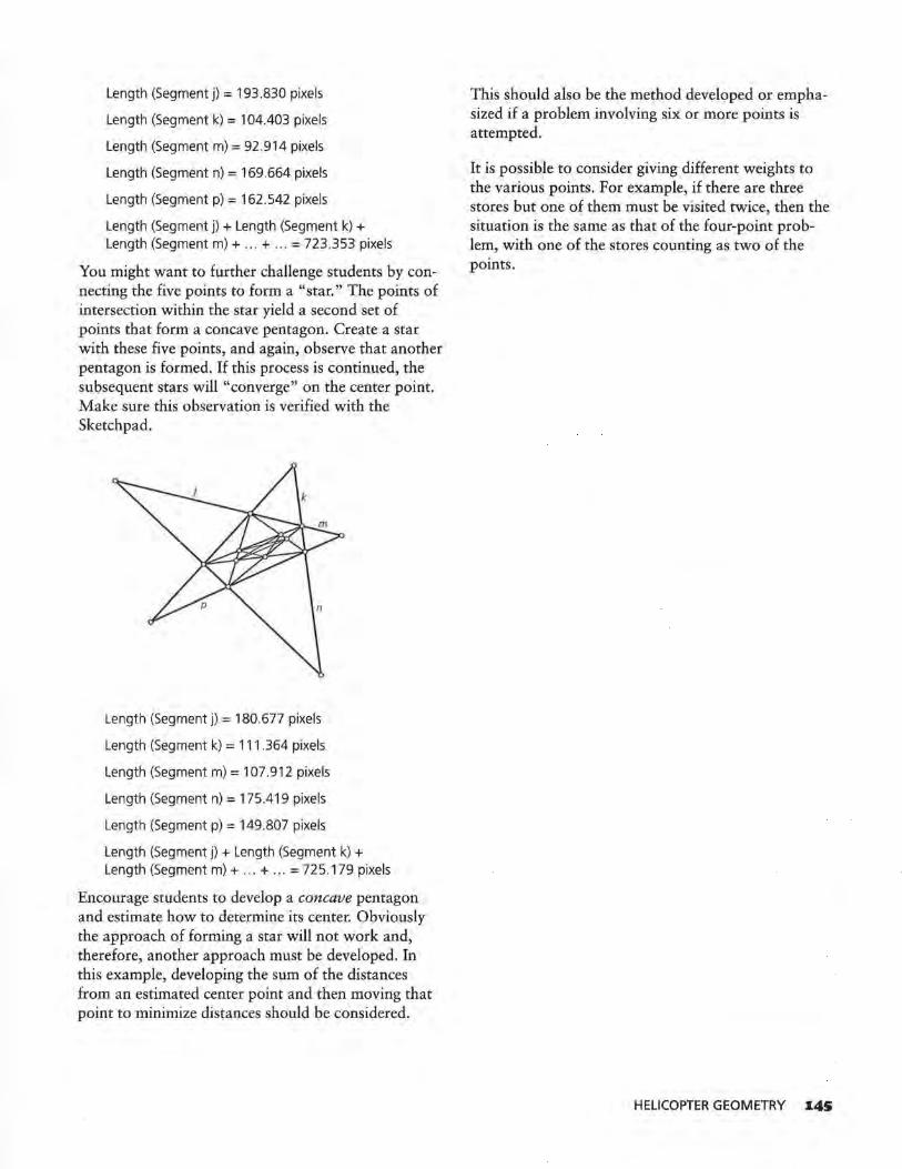
Length (Segment j) = 193 .830 pixels
Length (Segment k) = 104.403 pixels
Length (Segment m) = 92 .914 pixels
Length (Segment n) = 169.664 pixels
Length (Segment p) = 162.542 pixels
Length (Segment j) +Length (Segment k) + Length (Segment m) + ... + ... = 723.353 pixels
You might want to further challenge students by connecting the five points to form a "star." The points of intersection within the star yield a second set of points that form a concave pentagon. Create a star with these five points, and again, observe that another pentagon is formed. If this process is continued, the subsequent stars will "converge" on the center point. Make sure this observation is verified with the Sketchpad.
Length (Segment j) = 180.677 pixels
Length (Segment k) = 111.364 pixels
Length (Segment m) = 107.912 pixels
Length (Segment n) = 175.419 pixels
Length (Segment p) = 149.807 pixels
Length (Segment j) + Length (Segment k) + Length (Segment m) + ... + ... = 725.179 pixels
Encourage students to develop a concave pentagon and estimate how to determine its center. Obviously the approach of forming a star will not work and, therefore, another approach must be developed. In this example, developing the sum of the distances from an estimated center point and then moving that point to minimize distances should be considered.
This should also be the method developed or emphasized if a problem involving six or more points is attempted.
It is possible to consider giving different weights to the various points. For example, if there are three stores but one of them must be visited twice, then the situation is the same as that of the four-point problem, with one of the stores counting as two of the points.
HELICOPTER GEOMETRY X4S
LESSON 13: HELICOPTER GEOMETRY
STUDENT PAGE 118
146 LESSON 13
LESSON 13
Helicopter Geometry
What would be the advantages of using a helicopter instead of a truck to transport supplies from a distribution center to area stores?
What would the disadvantages be?
Determine the location on the plane that
minimizes the sum of distances to selected
points.
I n Lesson 12, the best location for a warehouse that served a group of stores was found under the condition that travel
was restricted along gridlines. The "center" turned out to involve the medians of the x- and y-coordinates of the stores. Suppose there is no restriction that travel must be along gridlines. Instead, supppse that you have a helicopter and can travel on a direct line to each point. It turns out that this makes the solution-the best location for the warehouse-harder to find!
INVESTIGATE
Consider three stores given by the points on the map shown below. The goal of the next set of problems is to find the best location for the wareh·ouse, given that you can fly directly from the warehouse to each point. In other, words, the warehouse does not have to be at the intersection of streets any more! Use the gridlines as a kind of graph paper to help keep track of locations on the map.
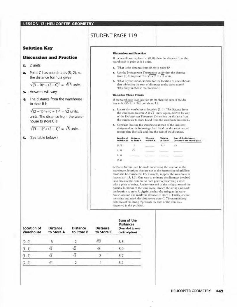
LESSON 13: HELICOPTER GEOMETRY
STUDENT PAGE 119
Solution Key
Discussion and Practice
x. 2 units
2. Point C has coordinates (3, 2), so the distance formula gives
'1 (3 - 0) 2 + (2 - 0)2 = -fi3 units.
~. Answers will vary.
4. The distance from the warehouse to store Bis
'1(2 -1)2+ (0-1)2 = "'12 units.
units. The distance from the warehouse to store C is
'1(3 - 1) 2 + (2 -1) 2 = ;/5 units.
s. (See table below.)
Location of Distance Distance Warehouse to Store A to Store B
(O, O) 3 2
(1 , 1) -rs -./2
(1, 2) -./2 -rs (2 , 2) -rs 2
Distance to Store C
-113
-rs 2
Dl4cu1don and Practtce
If the warehouse is placed at (0, 0), then the distance from the warehouse to point A is 3 units.
1. What is the distance from (0, 0) to point B?
z. Use the Pythagorean Theorem to verify that the distance from (0, 0) to point C is .,/3 2+2 2 = f13 units.
;t. What is your initial estimate for the location of a warehouse that minimizes the sum of distances to the three stores? Why did you choose that location?
Consider Three Points
If the warehouse is at location (0, 0), then the sum of the distances is .,/3 2+ 22 = f13, or about 3.6.
4. Locate the warehouse at location (1, 1 ). The distance from the warehouse to store A is {5 units (again, derived by way of the Pythagorea·n Theorem). Determine the distance from the warehouse to store B and from the warehouse to store C.
s. Consider locating the warehouse at each of the locations designated in the following chart. Find the distances needed to complete the table and find the sum of the distances.
location of Distance Distance Distance Sum of the Distances Warehouse to Store A to Store B to Store C (rounded to one declmal place)
(0. O) 8 6
(1. I) -./5 (1, 2)
(2, 2)
Before a decision can be made concerning the location of the warehouse, locations that are not at the intersection of grid lines must also be considered. For example, suppose the warehouse is located at (1.5, 1.5). One way to estimate the distances involved is to measure the distance to each point representing a store with a piece of string. Anchor one end of the string at one of the possible locations of the warehouse; stretch the string and mark the location to store A. Again, anchor the string at the warehouse location and mark the distance to store B. Finally, anchor the string and mark the distance to store C. The accumulated distances of the string represents the sum of the distances requested in this problem.
Sum of the Distances (Rounded to one
decimal place)
8.6
5.9
5.7
5.2
HELICOPTER GEOMETRY I47
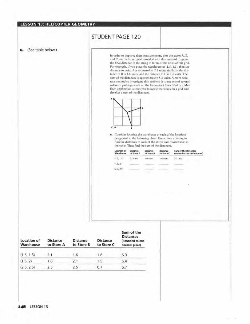
LESSON 13: HELICOPTER GEOMETRY
STUDENT PAGE 120
6. (See table below.)
Location of Distance Distance Warehouse to Store A to Store B
(1.5, 1.5) 2.1 1.6
(1.5, 2) 1.8 2.1
(2.5, 2.5) 2.5 2.5
~48 LESSON 13
In order to improve these measurements, plot the stores A, B, and C, on the larger grid provided with this material. Express the final distance of the string in terms of the units of this grid. For example, if you place the warehouse at (1.5, 1.5), then the distance to point A is estimated at 2.1 units; similarly, the distance to B is 1.6 units, and the distance to C is 1.6 units. The sum of the distances is approximately 5.3 units. A more accurate method to investigate this problem is to use one of several sofrware packages such as The Geometer's SketchPad or Cabri. Each application allows you to locate the stores on a grid and develop a sum of the distances.
c
\ (O,O)
&. Consider locating the warehouse at each of the locations designated in the following chart. Use a piece of string to find the distances to each of the stores and record those in the table. Then find the sum of the distances.
location of Distance Distance Distance Sum of the Distances Warehouse to Store A to Store B to StoreC (rounded to one decimal place)
(1 5, 1.5) 2 1 units 1.6 units 1 6 units 5 3 units
(1 5, 2) --- --- --- --(2 5, 2 5) --- --- --- --
Sum of the Distances
Distance (Rounded to one
to Store C decimal place)
1.6 5.3
1.5 5.4
0.7 5.7
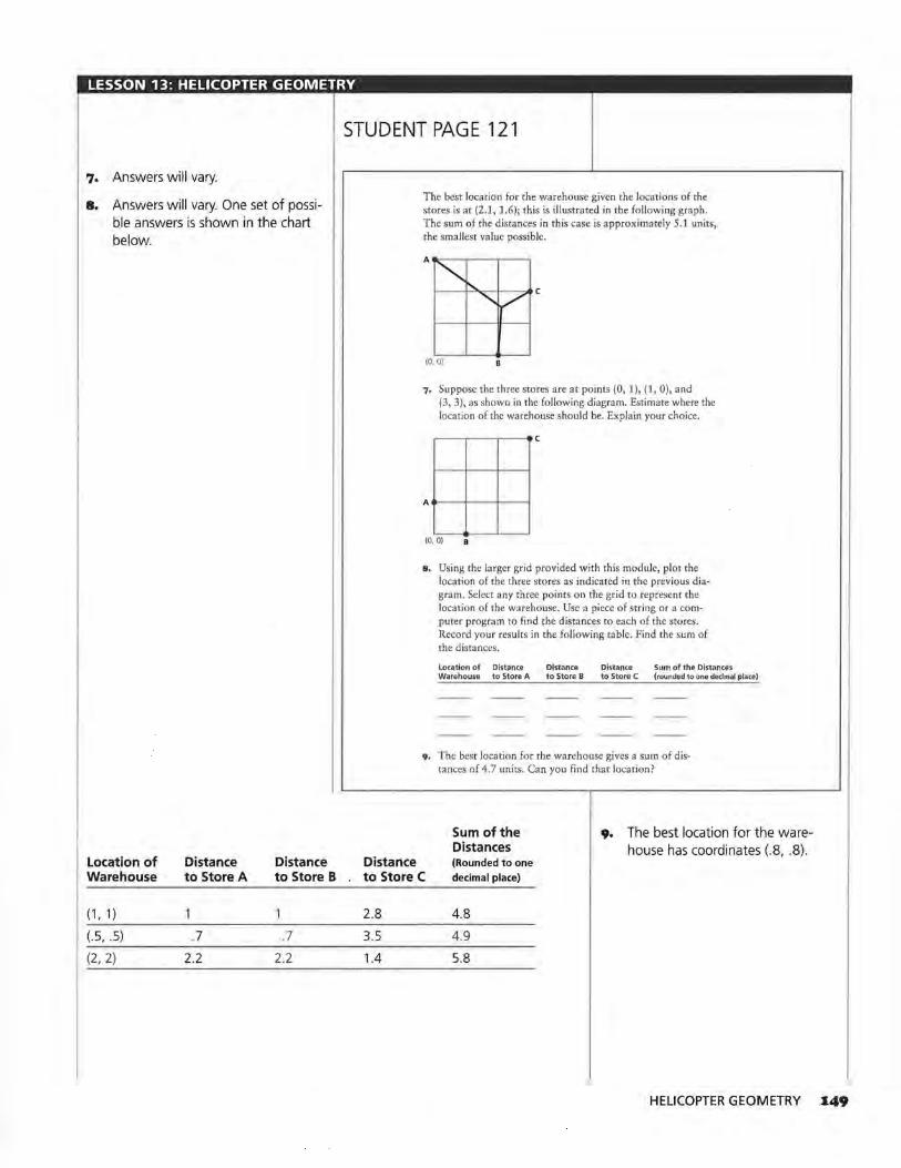
LESSON 13: HELICOPTER GEOMETRY
STUDENT PAGE 121
7. Answers will vary.
8. Answers will vary. One set of possible answers is shown in the chart below.
Location of Distance Distance Warehouse to Store A to Store B
(1, 1) 1
(. 5, .5) .7 .7 (2, 2) 2.2 2.2
Distance
The best location for the warehouse given the locations of the stores is at (2.1, 1.6); this is illustrated in the following graph. The sum of the. distances in this case is approximately 5.1 units, the smallest value possible.
(0, O)
7. Suppose the three stores are at points (0, 1), (1, 0), and (3, 3 ), as shown in the following diagram. Estimate where the location of the warehouse should be. Explain your choice .
.----.----,.-- - (
A - --t---t----t
(0, 0) B
8. Using the larger grid provided with this module, plot the location of the three stores as indicated in the previous diagram. Select any three points on the grid to represent the location of the warehouse. Use a piece of string or a computer program to find the distances to each of the stores. Record your results in the following table. Find the sum of the distances.
Location of Distance Distance Distance Sum of the Distances Warehouse to Store A to Store B to Store C (rounded to one declmal place)
9, The best location for the warehouse gives a sum of distances of 4.7 units. Can you find that location?
Sum of the 9. The best location for the ware-Distances house has coordinates (.8, .8). (Rounded to one
to Store C decimal place)
2.8 4.8
3.5 4.9
1.4 5.8
HELICOPTER GEOMETRY 149
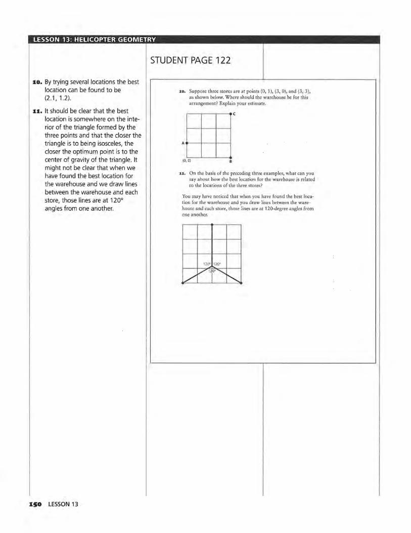
LESSON 13: HELICOPTER GEOMETRY
STUDENT PAGE 122
10. By trying several locations the best location can be found to be (2 .1, 1.2).
u. It should be clear that the best location is somewhere on the interior of the triangle formed by the three points and that the closer the triangle is to being isosceles, the closer the optimum point is to the center of gravity of the triangle. It might not be clear that when we have found the best location for the warehouse and we draw lines between the warehouse and each store, those lines are at 120° angles from one another.
150 LESSON 13
10. Suppose three stores are at points (0, 1), (3, 0), and (3, 3), as shown below. Where should the warehouse be for this arrangement? Explain your estimate.
-------c
A _ _ _.__ _ __,_ _ __.
(0, 0)
11. On the basis of the preceding three examples, what can you say about how the best location for the warehouse is related to the locations of the three stores?
You may have noticed that when you have found the best location for the warehouse and you draw lines between the warehouse and each store, those lines are at 120-degree angles from one another.
120° 120°
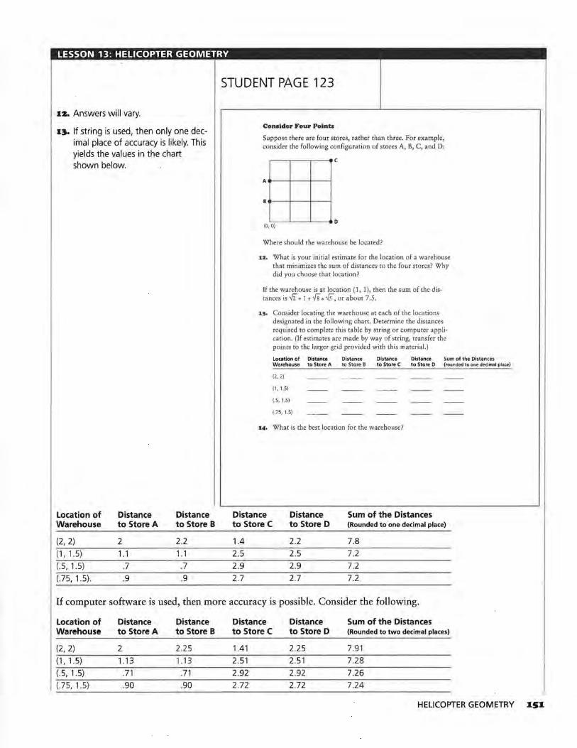
LESSON 13: HELICOPTER GEOMETRY
STUDENT PAGE 123
1z. Answers will vary.
1~. If string is used, then only one decimal place of accuracy is likely. This yields the values in the chart shown below.
Location of Distance Distance Warehouse to Store A to Store B
(2, 2) 2 2.2 (1, 1.5) 1.1 1.1 (.5, 1.5) .7 .7 (.75, 1.5). .9 .9
Consider Four Pobtts
Suppose there are four stores, rather than three. For example, consider the following configuration of stores A, B, C, and D:
....----.---~-- c
A- --+---+--t
8 - --+---+--!
(0.~0:-) -~-~-- D
Where should the warehouse be located?
12. What is your initial estimate for the location of a warehouse that minimizes the sum of distances to the four stores? Why did you choose that location?
If the warehouse is at location (1, 1), then the sum of the distances is {i + 1 + Ys + ../5, or about 7.5.
o. Consider locating the warehouse at each of the locations designated in the following chart. Determine the distances required to complete this table by string or computer application. (If estimates are made by way of string, transfer the points to the larger grid provided with this material.)
Location of Distance Distance Distance Distance Sum of the Distances Warehouse to Store A to Store 8 to Store C to Store D (rounded to one declmal place)
(2, 2)
(1, 1 5)
( 5, 1 5)
(.75, 1.5)
14. What is the best location for the warehouse?
Distance Distance Sum of the Distances to Store C to Store D (Rounded to one decimal place)
1.4 2.2 7.8
2.5 2.5 7.2
2.9 2.9 7.2 2.7 2.7 7.2
If computer software is used, then more accuracy is possible. Consider the following.
Location of Distance Distance Distance Distance Sum of the Distances Warehouse to Store A to Store B to Store C to Store D (Rounded to two decimal places)
(2, 2) 2 2.25 1.41 2.25 7.91
(1, 1.5) 1.13 1.13 2.51 2.51 7.28 (.5, 1.5) .71 .71 2.92 2.92 7.26 (.75, 1.5) .90 .90 2.72 2.72 7.24
HELICOPTER GEOMETRY ISI
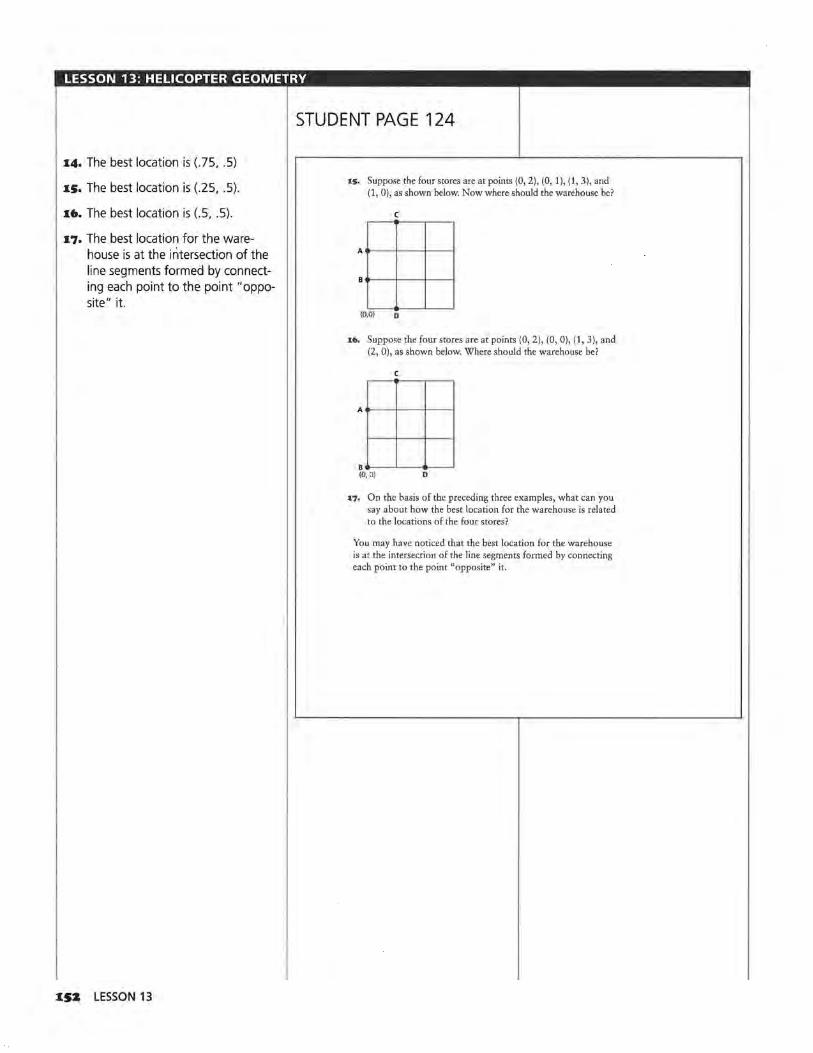
LESSON 13: HELICOPTER GEOMETRY
STUDENT PAGE 124
:14. The best location is (.75, .5)
1.5. The best location is (.25, .5).
a. The best location is (.5, .5).
17. The best location for the warehouse is at the intersection of the line segments formed by connecting each point to the point "opposite" it.
ISZ LESSON 13
IS. Suppose the four stores are at points (0, 2), (0, 1), (1, 3), and (1, 0), as shown below. Now where should the warehouse be?
c
A - --+----+----<
(0.0) D
I6. Suppose the four stores are at points (0, 2), (0, 0), (1, 3), and (2, 0), as shown below. Where should the warehouse be?
c
A - --1---1---t
s --~---~ (0,0) D
I7. On the basis of the preceding three examples, what can you say about how the best location for the warehouse is related to the locations of the four stores?
You may have noticed that the best location for the warehouse is at the intersection of the line segments formed by connecting each point to the point "opposite" it.
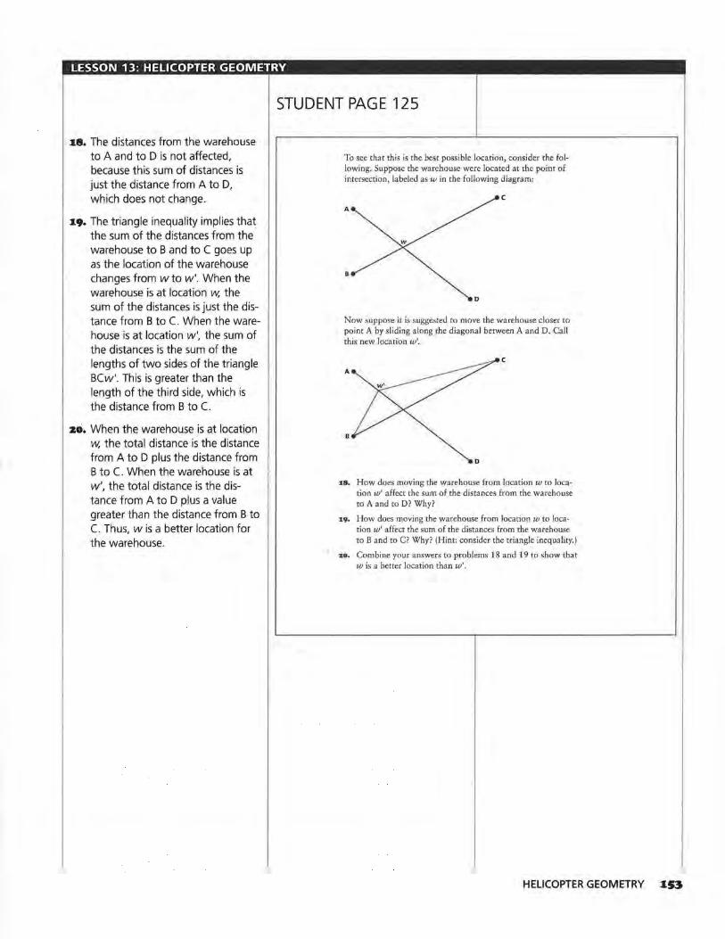
LESSON 13: HELICOPTER GEOMETRY
STUDENT PAGE 125
i:s. The distances from the warehouse to A and to D is not affected, because this sum of distances is just the distance from A to D, which does not change.
1:9. The triangle inequality implies that the sum of the distances from the warehouse to B and to C goes up as the location of the warehouse changes from w to w'. When the warehouse is at location w, the sum of the distances is just the distance from B to C. When the warehouse is at location w', the sum of the distances is the sum of the lengths of two sides of the triangle BCw'. This is greater than the length of the third side, which is the distance from B to C.
zo. When the warehouse is at location w, the total distance is the distance from A to D plus the distance from B to C. When the warehouse is at w', the total distance is the distance from A to D plus a value greater than the distance from B to C. Thus, w is a better location for the warehouse.
To see that this is the best possible location, consider the following. Suppose the warehouse were located at the point of intersection, labeled as w in the following diagram:
c A
B
D
Now suppose it is suggested to move the warehouse closer to point A by sliding along the diagonal between A and D. Call this new location w'.
c A
8
D
18, How does moving the warehouse from location w to location w' affect the sum of the distances from the warehouse to A and to D? Why?
19. How does moving the warehouse from location w to location w' affect the sum of the distances from the warehouse to Band to C? Why? (Hint: consider the triangle inequality.)
zo. Combine your answers to problems 18 and 19 to show that w is a better location than w'.
HELICOPTER GEOMETRY IS3
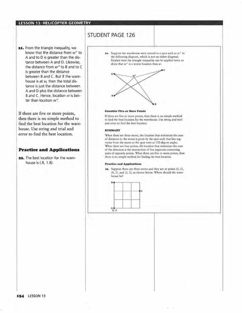
LESSON 13: HELICOPTER GEOMETRY
STUDENT PAGE 126
z1. From the triangle inequality, we know that the distance from w" to A and to D is greater than the distance between A and D. Likewise, the distance from w" to B and to C is greater than the distance between B and C. But if the warehouse is at w, then the total distance is just the distance between A and D plus the distance between B and C. Hence, location w is better than location w''.
If there are five or more points, then there is no simple method to find the best location for the warehouse. Use string and trial and error to find the best location.
Practice and Applications
zz. The best location for the warehouse is (.8, 1.8).
IS4 LESSON 13
2:1. Suppose the warehouse were moved to a spot such as w" in the following diagram, which is not on either diagonal. Explain how the triangle inequality can be applied twice to show that w" is a worse location than w.
c A
Consider Five or More Points
If there are five or more points, then there is no simple method to find the best location for the warehouse. Use string and trial and error to find the best location.
SUMMARY
When there 'are three stores, the location that minimizes the sum of distances to the stores is given by the spot such that line segments from the stores to the spot meet at 120-degree angles. When there are four points, the location that minimizes the sum of the distances is the intersection of line segments connecting pairs of opposite points. When there are five or more points, then there is no simple method for finding the best location.
Practice and Applications
22. Suppose there are three stores and they are at points (0, 0), (0, 3), and (3, 2), as shown below. Where should the warehouse be?
B - -.....---,..--,
--!--·>----- c
A--~-~-~
(0, O)
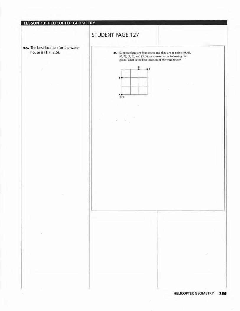
LESSON 13: HELICOPTER GEOMETRY
STUDENT PAGE 127
z~. The best location for the warehouse is (1.7, 2.5). ZJ,. Suppose there are four stores and they are at points (0, 0),
(0, 2), (2, 3), and (3, 3), as shown on the following diagram. What is the best location of the warehouse?
c ~-----o
B - --1-- +-----i
... ---'-----'----' (0, 0)
HELICOPTER GEOMETRY ISS
LESSON 14
The Worst-Case Scenario! Materials: rulers, Activity Sheet 13, Unit V Quiz
Technology: A scientific calculator or graphing calculator will
do, but a geometry software package such as Geometer's
SketchPad or Cabri is preferable.
Pacing: 2 class sessions
Overview
The Worst-Case Scenario! is an interesting concept that will challenge some students. The problems are designed so that students are presented scattered points on a grid. What center point would minimize the distance needed to travel to the farthest location in this scatter? In other words, where would a center be located to minimize the worst-case scenario? The lesson develops this idea with the students using a "shrinking and sliding" process. Place a constructed circle over the entire scatter of points. As the student shrinks this circle down, it will eventually touch one of the points of the scatter. When this happens, slide the circle so that all of the points are again within the smaller circle. Then start shrinking the circle down again. Repeat this process until it is no longer possible to move the circle without placing points outside the circle. The center of this circle is the estimate of the worst-case scenario. Visualizing this process is again best developed using one of the geometry software packages previously mentioned.
Teaching Notes
The development of the prepared lesson is again designed for the situation in which access to computer software is limited. The specific problems presented in the student materials are arranged to guide the students through the process. Included in this teacher's edition, however, is a demonstration of the "shrinkand-slide" process using the Geometer's Sketchpad.
IS6 LESSON 14
The explanation provides suggestions on how to set up the problems. Specific details related to using the software are not developed for similar reasons mentioned in the opening comments of Lesson 13.
Follow-Up
Several applications of "minimizing the worst case" could be presented to students. One discussion that could be particularly relevant is a discussion of insurance rates. The goal of developing insurance rates is to provide for the "worst case" (i.e., car completely wrecked, house completely destroyed). It is also, however, the goal to determine this coverage for a minimum cost to the consumer. Balancing these needs is another example of determining a special type of center! Topics illustrating this concept are found in several business applications.
Technology
As with Lesson 13, the Geometer's Sketchpad or similar software is helpful when exploring the ideas presented in this lesson. The first part of the lesson (problems 1-9) deals with points on a number line and makes no use of software. However, the second part of the lesson (Problems 10-14) concerns points on the plane. Here software is very useful.
For example, you can use the Geometer's Sketchpad to carry out the "shrink-and-slide" method presented in problem 14 as follows. In the diagram below we have placed eight points on the plane using the
Sketchpad. We wish to find the center point that minimizes the distance to the farthest point. The first step is to choose the circle tool, put the center of the circle at a sensible guess for the solution, and expand the circle until it completely surrounds the eight points. Note that this will add two points to the sketch: the center of the circle and a "handle" that allows you to later shrink the circle.
0
0
0 center
0
Now grab the handle (use the pointing tool) and shrink the circle until it touches one of the eight points. In the diagram below, the circle touches the point at the lower left part of the sketch.
0
0
0
0 center
0
Now grab the circle by its edge, rather than by the handle, and slide it until there is white space between the circle and each point.
0
0
0
0
Shrink the circle, as before, until it touches a point. Then slide it; then shrink it; then slide it, etc. Eventually no more sliding or shrinking is possible. When this happens you are finished. The solution to the .Problem is the center of the circle.
0
0
0 center
0
0
The process of finding the center of a circle by the "shrinking-and-sliding" process approximates the center of a well-known circle involved in geometric constructions. Most scatters of points finally shrink on the three points farthest out. The triangle formed by these three points and the resulting circumscribed circle would locate the point (i.e., circle's center) that minimizes the distances to the farthest points. This circle has a constructed center as the intersection of the perpendicular bisectors. The connection between our shrink-and-slide circle and this circle is exciting; however, this connection is only for acute or right triangles. For obtuse triangles, the shrink-and-slide circle is different.
The following graph shows the construction of the circumscribed circle for the example with eight points presented above:
THE WORST-CASE SCENARIO! IS7
The center of the perpendicular bisectors is labeled above. This is also the center of the smallest circle in our shrink-and-slide process. In this case, the center is the point that minimizes the farthest distance problem.
Obtuse Triangles It may be that the three points toward the "edge" of the scattering of points form an obtuse triangle, as in the diagram that follows. The center for a circumscribed circle of the three points labeled as A, B, and C is center 1. This is not the center that minimizes the distances to the farthest points. Center2 is the center of the circle resulting from our shrink-and-slide discussion. Note its relationship to the points and to the circumscribed circle.
A
IS8 LESSON 14
LESSON 14: THE WORST-CASE SCENARIO!
STUDENT PAGE 128
LESSON 14
The Worst-Case Scenario!
Jacksonville, Florida, is a "port of entry," a U.S. town that receives cars imported from other countries. Would you expect the price of a new car in Jacksonville to be the same as the price of the same model car in Minneapolis?
You have agreed to buy a new car, but the dealer currently does not have the car in the color you want. How does the dealer find and get the car you want?
• :
Calculate the value that minimizes the greatest
distance.
R econsider the warehouse problem presented in Lesson 11. Suppose that instead of stocking every store at the end of
the week, a different delivery problem is presented. In this new situation, stores call the warehouse when a sale has been made; it is the company's goal to deliver that product from the central warehouse to the store as soon as possible. For example, car dealerships cannot stock every model in every color combination. Once a customer has selected a car with specific features and in a certain color, someone from the central storage warehouse must drive the customer's selection to the dealership. If this is your job, you hope the dealership is close to the "central" warehouse. On some unlucky days, you will be required to travel to the dealership that is farthest from the central warehouse. Thus, the car company considers locating the central warehouse so that the distance to the farthest dealership is minimized.
INVESTIGATE
New Car Delivery
This problem and its solution are different from the problem and solution presented in Lesson 11. In Lesson 11, the goal
THE WORST-CASE SCENARIO! 159
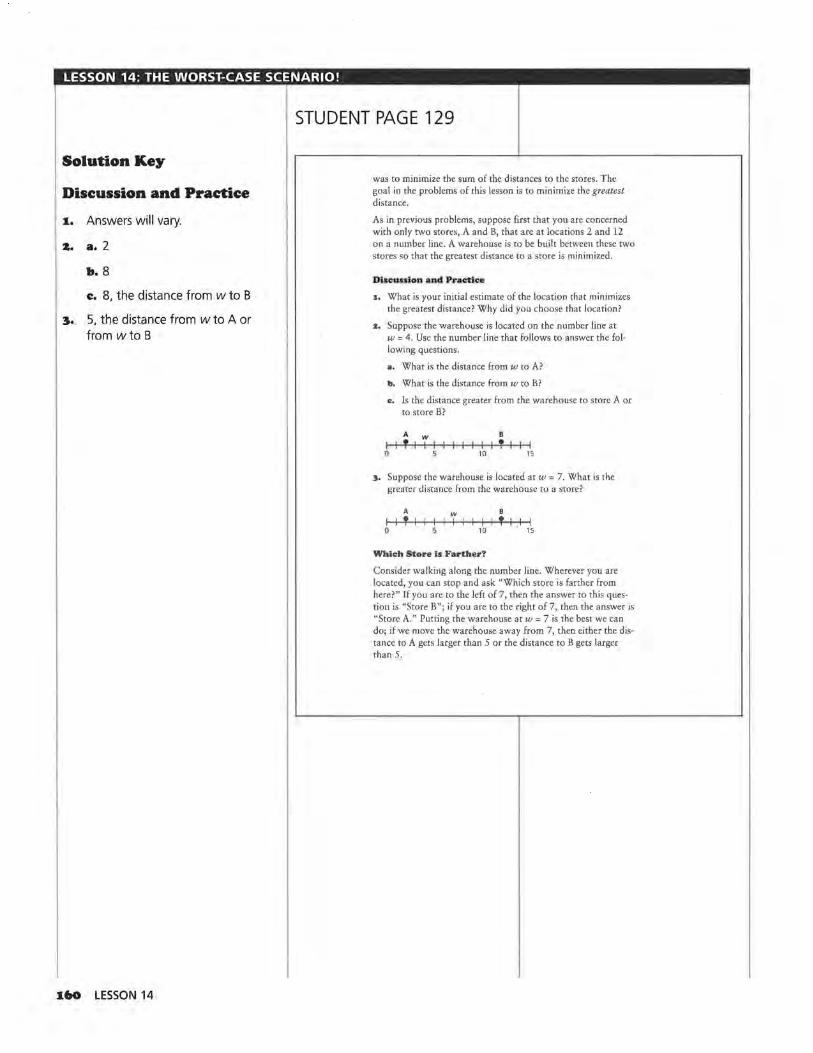
LESSON 14: THE WORST-CASE SCENARIO!
STUDENT PAGE 129
Solution Key
Discussion and Practice
1. Answers will vary.
z. a. 2
"· 8 c. 8, the distance from w to B
~. 5, the distance from w to A or from wto B
1fl0 LESSON 14
was to minimize the sum of the distances to the stores. The goal in the problems of this lesson is to minimize the greatest distance.
As in previous problems, suppose first that you are concerned with only two stores, A and B, that are at locations 2 and 12 on a number line. A warehouse is to be built between these two stores so that the greatest distance to a store is minimized.
Dbcu.ulon and Practice
1. What is your initial estimate of the location that minimizes the greatest distance? Why did you choose that location?
:a. Suppose the warehouse is located on the number line at w = 4. Use the number line that follows to answer the following questions.
a. What is the distance from w to A?
b. What is the distance from w to B?
e, Is the distance greater from the warehouse to store A or to store B?
A
I I T w B I 1 I I l I I l T I I I
0 5 10 15
~. Suppose the warehouse is located at w = 7. What is the greater distance from the warehouse to a store?
A
I I T I I w e
I I I I I I T I .1 I 0 10 15
Which Store is Farther?
Consider walking along the number line. Wherever you are located, you can stop and ask "Which store is farth er from here?" If you are to the left of 7, then the answer to this question is "Store B"; if you are to the right of 7, then the answer is "Store A." Putting the warehouse at w = 7 is the best we can do; if we move the warehouse away from 7, then either the distance to A gets larger than 5 or the distance to B gets larger than 5.
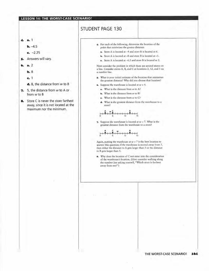
LESSON 14: THE WORST-CASE SCENARIO!
STUDENT PAGE 130
4. a. 1
b. -4.5
c. -2.25
s. Answers will vary.
6. a. 2
b.8
c. 1
d. 8, the distance from w to B
7. 5, the distance from w to A or from wto B
8. Store C is never the store farthest away, since it is not located at the maximum nor the minimum.
4, For each of the following, determine the location of the point that minimizes the greater distance:
a. Store A is located at -4 and store Bis located at 6.
b. Store A is located at-8 and store Bis located at -1.
c. Store A is located at -6.5 and store B is located at 2.
Now consider the problem in which there are several stores on a line. Consider stores A, B, and Cat locations 2, 12, and 5 on a number line.
5, What is your initial estimate of the location that minimizes the greatest distance? Why did you choose that location?
f>, Suppose the warehouse is located at w = 4.
a. What is the distance from w to A?
b. What is the distance from w to B?
c. What is the distance from w to C?
d. What is the greatest distance from the warehouse to a store?
A w C B
I T I T I I I I I I T I I I 0 5 10 15
7. Suppose the warehouse is located at w = 7. What is the greatest distance from the warehouse to a store?
A C w B
I T I I T I I I I I I T I I I 0 , 10 15
Again, putting the warehouse at w = 7 is the best location to answer this question; if the warehouse is moved away from 7, then either the distance to A gets larger than 5 or the distance to B gets larger than 5.
8. Why does the location of C not enter into the consideration of the warehouse's location. (Hint: consider walking along the number line asking yourself, "Which store is farthest away from me?")
THE WORST-CASE SCENARIO!
LESSON 14: THE WORST-CASE SCENARIO!
STUDENT PAGE 131
9. a. 1.5
b. Store D must be at location 9. The midrange is 4, since that is the location of the dealership, and the minimum is -1. Thus, the maximum must be 9, since (-1 + 9)/2 = 4.
I6Z LESSON 14
What happens if there are n stores on a number line? Consider stores P 1, P 2, ••• , P" on a number line.
r r r
As you walk along this number line, there are only two possible answers to your favorite question, "Which store is farthest from me?" Sometimes store P1 is the most distant store and sometimes store P n is the most distant store. If you start to the left of P 1 and walk toward the right, then P" is the most distant store for the first part of the walk. Eventually P 1 becomes the most distant point. Where does this switch happen?
The midrange is defined to be:
Minimum value + Maximum value 2
This is another type of center and is the solution to the problem for points located on a number line.
9. Use the midrange to determine the location on a number line of the points requested in the following statements:
a. Determine the location of point w that minimizes the greatest distance from point w to any one of the following stores: store A at -5, store Bat -2, store Cat 3, and store D at 8.
b. The location of the central distribution warehouse for four car dealerships (namely A, B, C, and D) is at the location of 4 on a number line. Store A is located at -1, store B at 2 , and store C at 5. Determine the location of store D. Explain how you determined your solution to this statement.
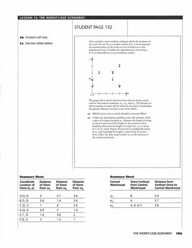
LESSON 14: THE WORST-CASE SCENARIO!
STUDENT PAGE 132
10. Answers will vary.
11. See two tables below.
Summary Sheet
Coordinate Distance Distance Distance Location of of Store of Store of Store Store (x, y) from w1 from w2 from w3
A(O, 5) 3 5.7 3.6
B (5, O) 5.4 1.4 3.6
c (0, 1) 1 4 3.6
D(4, 4) 4.5 3 1.4
E (1, 3) 1.4 3.6 2
F (3, 2) 3 1.4
Now consider a more realistic setting in which the locations of the stores do not fit on a simple number line. A more appropriate representation of the stores is a set of points on a twodimensional map. Consider the representation of six stores, A-F, as illustrated on an xy-coordinate system:
A 5
w, ··U ·
c ~
(0,0)
E
• W3 • F
•
I
D
•
w, •
8 5
The graph above shows three locations that are being considered for the central warehouse: w 1, w2, and w3• The decision of which location to select will be based on the goal of minimizing the greatest distance traveled to any of the stores.
:10. Which location do you think should be selected? Why?
u. Collect the information needed to make this decision. Hold a piece of string at location w1• Measure the length of string to store A and record this length on the summary sheet. Similarly, determine the length of string from w 1 to stores B, C, D, E, and F. Repeat this process by holding the string at w2 and recording the length to each of the six stores. Also, collect the data using location w3 as the location of the central warehouse.
Summary Sheet
Central Store Farthest Warehouse from Central
Warehouse
W1 B
W2 A
W3 A, B, or C
Distance from Farthest Store to Central Warehouse
5.4
5.7
3.6
THE WORST-CASE SCENARIO! I63
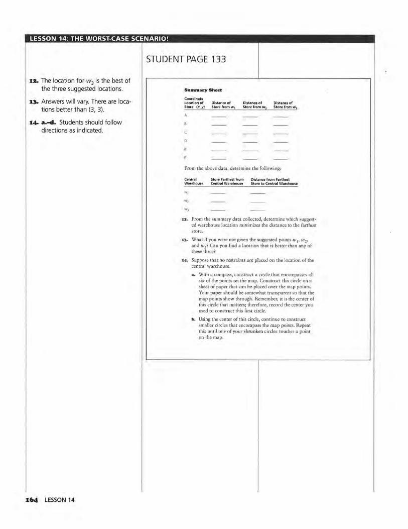
LESSON 14: THE WORST-CASE SCENARIO!
STUDENT PAGE 133
u. The location for w3 is the best of the three suggested locations.
i::i. Answers will vary. There are locations better than (3, 3).
1:4. a.-d. Students should follow directions as indicated.
I64 LESSON 14
Summary Sheet
Coordinate location of Distance of Distance of Distance of Store (x, y) Store from w1 Store from w2 Store from w3
A
c
D
From the above data, determine the following:
Central Store Farthest from Distance from Farthest Warehouse Central Warehouse Store to Central Warehouse
w,
w,
1z. From the summary data collected, determine which suggested warehouse location minimizes the distance to the farthest store.
13. What if you were not given the suggested points w1, w2,
and w3? Can you find a location that is better than any of these three?
14. Suppose that no restraints are placed on the location of the central warehouse.
a. With a compass, construct a circle that encompasses all six of the points on the map. Construct this circle on a sheet of paper that can be placed over the map points. Your paper should be somewhat transparent so that the map points show through. Remember, it is the center of this circle that matters; therefore, record the center you used to construct this first circle.
b. Using the center of this circle, continue to construct smaller circles that encompass the map points. Repeat this until one of your shrunken circles touches a point on the map.
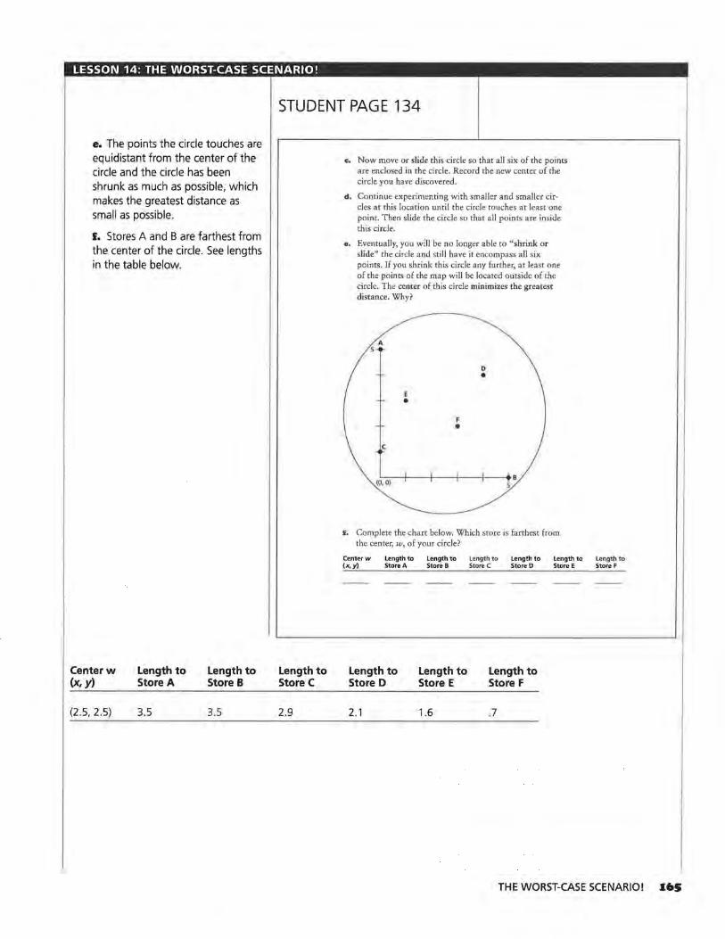
LESSON 14: THE WORST-CASE SCENARIO!
STUDENT PAGE 134
e. The points the circle touches are equidistant from the center of the circle and the circle has been shrunk as much as possible, which makes the greatest distance as small as possible.
f. Stores A and B are farthest from the center of the circle. See lengths in the table below.
Centerw {x, y)
(2.5, 2.5)
Length to Store A
3.5
length to Store B
3.5
Length to Store C
2.9
c. Now move or slide this circle so that all six of the points are enclosed in the circle. Record the new center of the circle you have discovered.
d. Continue experimenting with smaller and smaller circles at this location until the circle touches at least one point. Then slide the circle so that all points are inside this circle.
e. Eventually, you wlll be no longer able to "shrink or slide" the circle and still have it encompass all six points. If you shrink this circle any further, at least one of the points of the map will be located outside of the circle. The center of this circle minimizes the greatest distance. Why?
f. Complete the chart below. Which store is farthest from the center, w, of your circle?
Center w Length to Length to Length to Length to Length to Length tO (x, y) Store A Store B Store C Store D Store E Store F
length to Store D
2.1
Length to Store E
1.6
Length to Store F
.7
THE WORST-CASE SCENARIO! I65
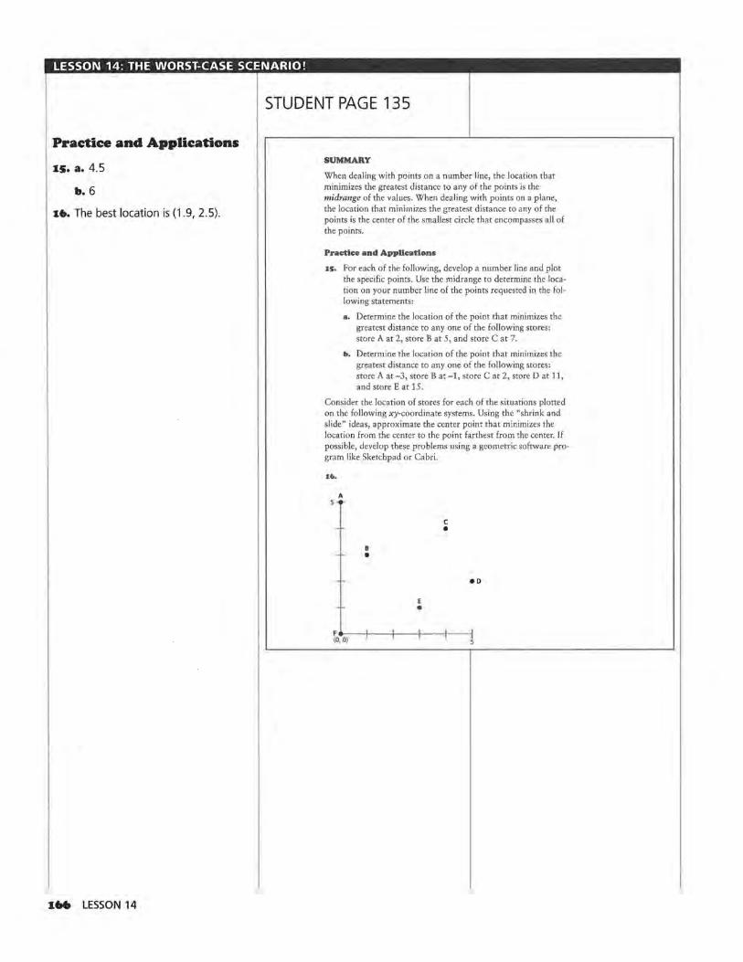
LESSON 14: THE WORST-CASE SCENARIO!
STUDENT PAGE 135
Practice and Applications
15. a. 4.5
b. 6
1•. The best location is (1 .9, 2.5) .
~66 LESSON 14
SUMMARY
When dealing with points on a number line, the location that minimizes the greatest distance to any of the points is the midrange of the values. When dealing with points on a plane, the location that minimizes the greatest distance to any of the points is the center of the smallest circle that encompasses all of the points.
Practice and Applications
15. For each of the following, develop a number line and plot the specific points. Use the midrange to determine the location on your number line of the points requested in the following statements:
a. Determine the location of the point that minimizes the greatest distance to any one of the following stores: store A at 2, store Bat 5, and store Cat 7.
b. Determine the location of the point that minimizes the greatest distance to any one of the following stores: store A at -3, store B at -1, store C at 2, store D at 11, and store Eat 15.
Consider the location of stores for each of the situations plotted on the following xy-coordinate systems. Using the "shrink and slide" ideas, approximate the center point that minimizes the location from the center to the point farthest from the center. If possible, develop these problems using a geometric software program like Sketchpad or Cabri.
u ..
A s
e -- . E
•
c •
aD
F e-~--t-' ~--t-'~--t-' ~-i--'~-t' (0,0) t t t I S
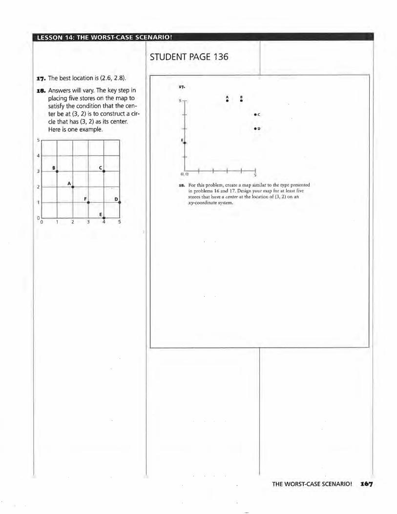
LESSON 14: THE WORST-CASE SCENARIO!
STUDENT PAGE 136
1.7. The best location is (2.6, 2.8).
1.8. Answers will vary. The key step in placing five stores on the map to satisfy the condition that the center be at (3, 2) is to construct a circle that has (3, 2) as its center. Here is one example.
5
4
3
2
0 0
B
A
2
c
F D
E
3 4 5
5-
--
I
(0, O) I I I
A
•
'
B
•
' I
ec
eo
' 5
18. For this problem, create a map similar to the type presented in problems 16 and 17. Design your map for at least five stores that have a center at the location of (3, 2) on an xy-coordinate system,
THE WORST-CASE SCENARIO! 1•7


Teacher Resources

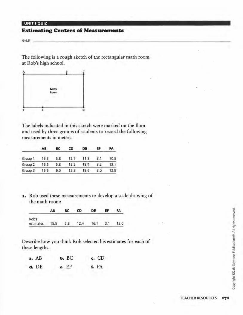
UNIT I QUIZ
Estimating Centers ol Measurements
NAME
The following is a rough sketch of the rectangular math room at Rob's high school.
A
F E
Math Room
B c
D
The labels indicated in this sketch were marked on the floor and used by three groups of students to record the following measurements in meters.
AB BC CD DE EF FA
Group 1 15.3 5.8 12.7 11.3 3.1 10.8
Group 2 15.5 5.8 12.2 18.4 3.2 13.1
Group 3 15.6 6.0 12.3 18.6 3.0 12.9
I. Rob used these measurements to develop a scale drawing of the math room:
AB BC CD DE EF FA
Rob's estimates 15.5 5.8 12.4 16.1 3.1 13.0
Describe how you think Rob selected his estimates for each of these lengths.
a. AB
d. DE
b. BC
e. EF
c. CD
I. FA
TEACHER RESOURCES I7I
:J 0 E >, QJ Vl
QJ -;u 0 @ ..,, L Ol ·~ Q_ 0 u
z. What properties of a rectangle could be used to evaluate the accuracy of Rob's estimates?
3. How do you know a scale drawing of the math room using Rob's estimates will be inaccurate?
4. Develop a scale drawing of the math room using Rob's estimates and the scale 1 cm= 1 meter.
s. Identify one of Rob's estimates you think is an inaccurate estimate of the data set.
a. Describe why you selected this measurement.
b. What value would you use for this measurement? Why?
•· Re-examine the measurements recorded by the three groups. Select an estimate for each of the labeled distances. Copy and complete the following chart indicating your estimates.
Your estimates
AB BC CD DE EF FA
7. Develop a scale drawing of the math room using your estimates and the scale of 1 cm= 1 meter.
8. Do you think your drawing is a more accurate representation of the math room than Rob's drawing? Why or why not?
17Z UNIT I QUIZ
<.(
~ c 0 ·.;:::;
-~ JS :J
CL
:; 0 E >, (])
VI (])
<ii 0 @ ..., ..c
°' -~ 0 u
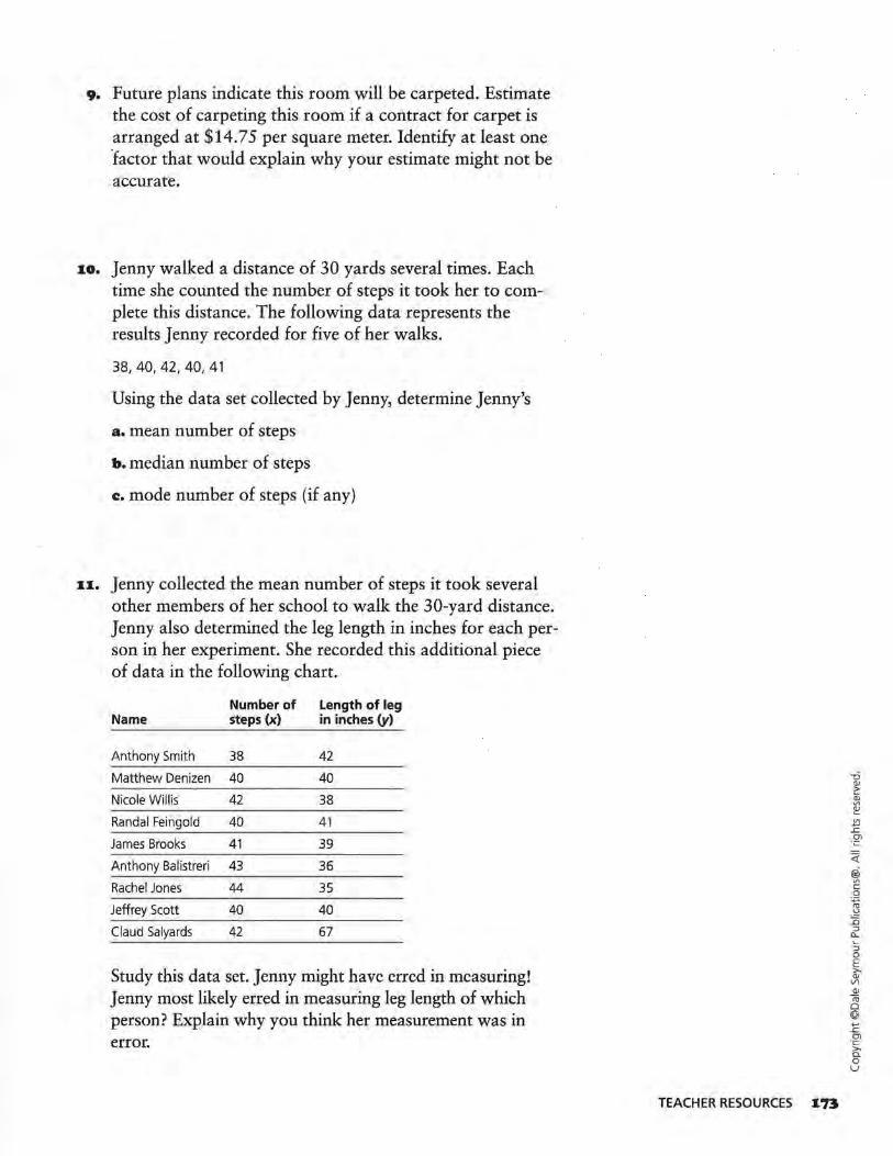
9. Future plans indicate this room will be carpeted. Estimate the cost of carpeting this room if a contract for carpet is arranged at $14.75 per square meter. Identify at least one factor that would explain why your estimate might not be accurate.
10. Jenny walked a distance of 30 yards several times. Each time she counted the number of steps it took her to complete this distance. The following data represents the results Jenny recorded for five of her walks.
38,40,42,40,41
Using the data set collected by Jenny, determine Jenny's
a. mean number of steps
b. median number of steps
c. mode number of steps (if any)
11. Jenny collected the mean number of steps it took several other members of her school to walk the 30-yard distance. Jenny also determined the leg length in inches for each person in her experiment. She recorded this additional piece of data in the following chart.
Number of Length of leg Name steps (x) in inches (y)
Anthony Smith 38 42
Matthew Denizen 40 40
Nicole Willis 42 38
Randal Feingold 40 41
James Brooks 41 39
Anthony Balistreri 43 36
Rachel Jones 44 35
Jeffrey Scott 40 40
Claud Salyards 42 67
Study this data set. Jenny might have erred in measuring! Jenny most likely erred in measuring leg length of which person? Explain why you think her measurement was in error.
TEACHER RESOURCES 173
<!: @ "' c 0
·.;::;
-~ ::0 ::J
CL
::J 0 E >Cl)
V1 Cl)
Iii 0 @ ..., L Ol
·~ 0 u
1.2. Develop a scatter plot of the data given in problem 11. Use a coordinate grid similar to the one below. Do not include any values from the data set you think represent an error in Jenny's measurement.
· ~
-
1.3. Do you think you could estimate a person's leg length based on the number of steps it took this person to walk 30 yards? Why or why not?
J.4. Estimate Jenny's leg length. How did you determine your estimate?
J.74 UNIT I QUIZ
<(
@) Vl c 0
·.;::; re
.!:! ::0 :J 0..
:J 0 E it'
V1 QI
ro Cl @ .... ..c 01
-~ 0 u
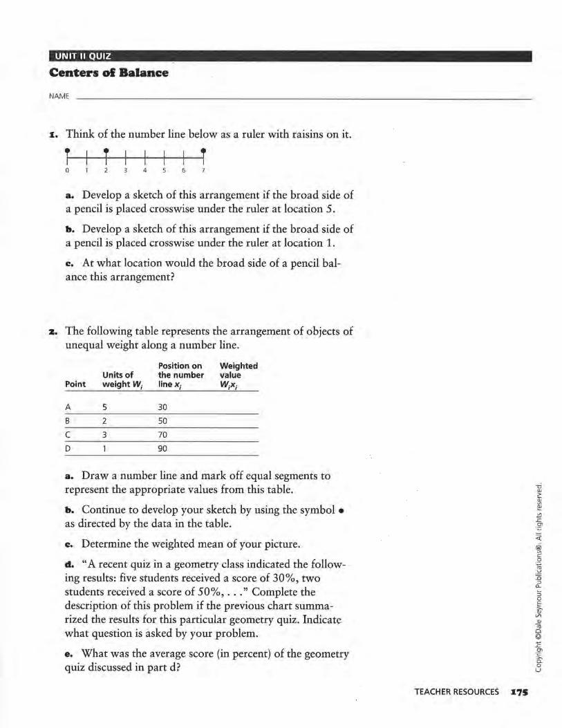
UNIT II QUIZ
Centers ol Balance
NAME
I. Think of the number line below as a ruler with raisins on it.
T T I I I I T 0 2 3 4 5 6 7
a. Develop a sketch of this arrangement if the broad side of a pencil is placed crosswise under the ruler at location 5.
b. Develop a sketch of this arrangement if the broad side of a pencil is placed crosswise under the ruler at location 1.
c. At what location would the broad side of a pencil balance this arrangement?
z. The following table represents the arrangement of objects of unequal weight along a number line.
Position on Weighted Units of the number value
Point weight W; linex; W;X;
A 5 30
B 2 50
c 3 70
D 90
a. Draw a number line and mark off equal segments to represent the appropriate values from this table.
b. Continue to develop your sketch by using the symbol • as directed by the data in the table.
c. Determine the weighted mean of your picture.
d. "A recent quiz in a geometry class indicated the following results: five students received a score of 30%, two students received a score of 50%, ... " Complete the description of this problem if the previous chart summarized the results for this particular geometry quiz. Indicate what question is asked by your problem.
e. What was the average score (in percent) of the geometry quiz discussed in part d?
TEACHER RESOURCES I7S
<(
@i Vl c 0
·.;:::; ro .~ 15 ::J
CL
::; 0 E >QJ VI
QJ cu 0 @ ..., ..c Ol ·~ 0.. 0 u
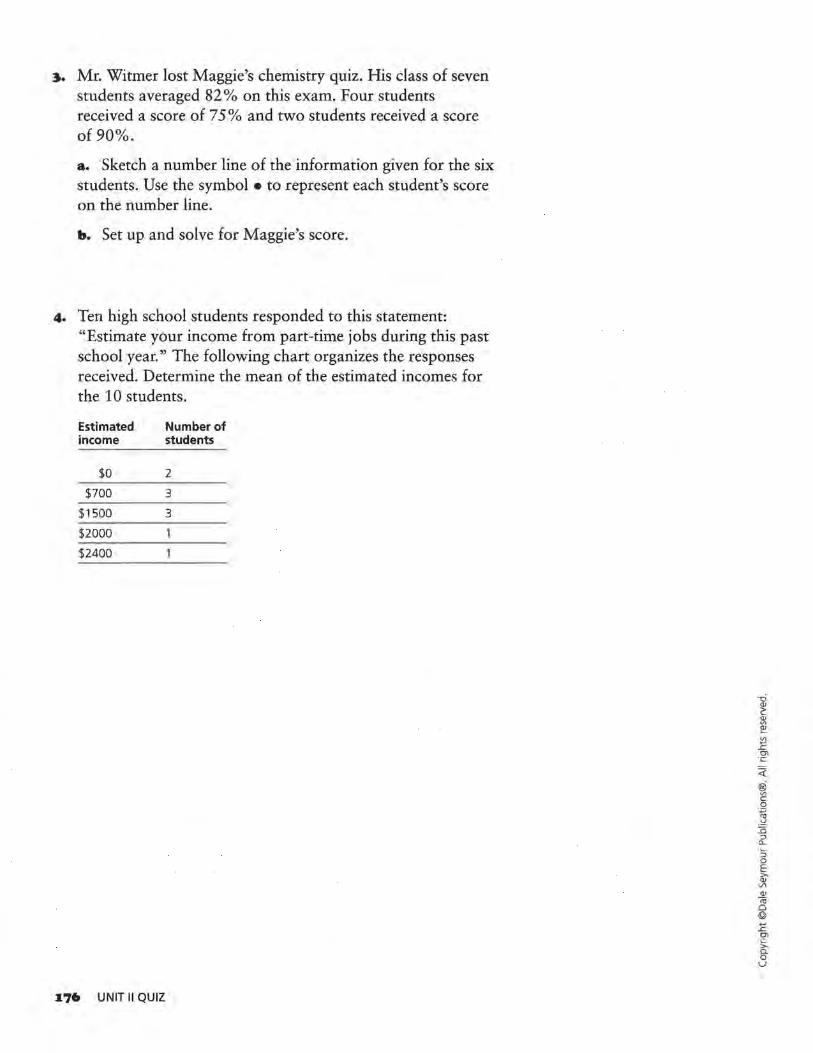
3. Mr. Witmer lost Maggie's chemistry quiz. His class of seven students averaged 82 % on this exam. Four students received a score of 75% and two students received a score of 90%.
a. Sketch a number line of the information given for the six students. Use the symbol • to represent each student's score on the number line.
b. Set up and solve for Maggie's score.
4. Ten high school students responded to this statement: "Estimate your income from part-time jobs during this past school year." The following chart organizes the responses received. Determine the mean of the estimated incomes for the 10 students.
Estimated Number of income students
$0 2
$700 3
$1500 3
$2000
$2400
176 UNIT II QUIZ
<(
® Vl c 0 ·.;:::;
-~ :0 ::l
CL
:; 0 E >OJ VI
OJ ro 0 @ +-' .£ Ol -~ a.. 0 u
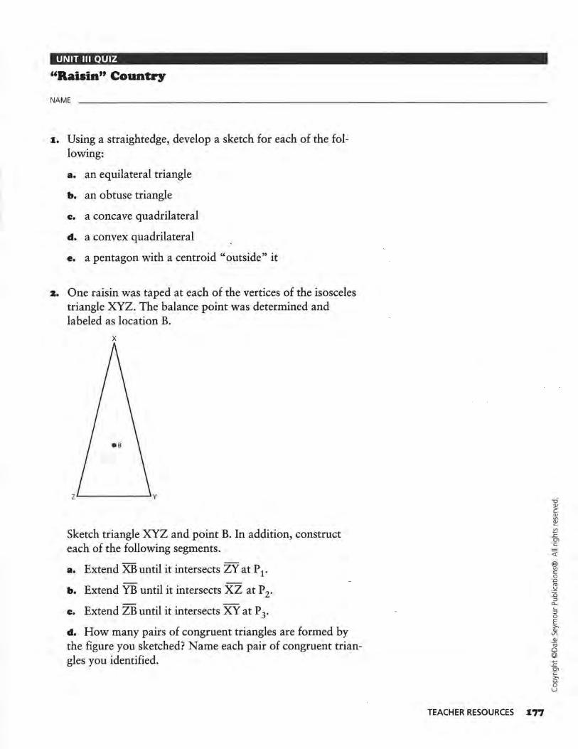
UNIT Ill QUIZ
"Raisin" Country
NAME
1. Using a straightedge, develop a sketch for each of the following:
a. an equilateral triangle
b. an obtuse triangle
c. a concave quadrilateral
d. a convex quadrilateral
e. a pentagon with a centroid "outside" it
z. One raisin was taped at each of the vertices of the isosceles triangle XYZ. The balance point was determined and labeled as location B.
x
Sketch triangle XYZ and point B. In addition, construct each of the following segments.
a. Extend XB until it intersects ZY at P 1.
b. Extend YB until it intersects XZ at P 2.
c. Extend ZB until it intersects XY at P 3•
d. How many pairs of congruent triangles are formed by the figure you sketched? Name each pair of congruent triangles you identified.
TEACHER RESOURCES 177
~
® Vl c 0 ·.;:::;
"' .!:! J5
" Cl..
::; 0 E ~
Vl QJ
Iii Cl @ .... ..c Ol
-~ 0 u
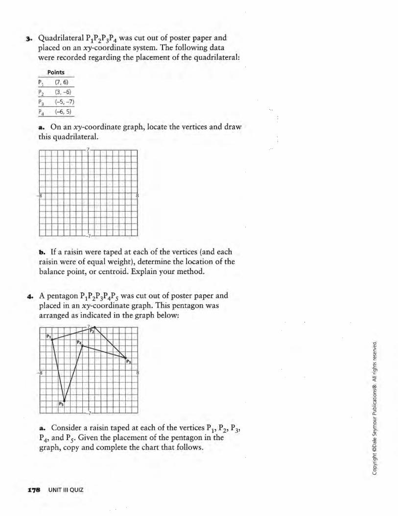
~. Quadrilateral P1P2P3P4 was cut out of poster paper and placed on an xy-coordinate system. The following data were recorded regarding the placement of the quadrilateral:
Points
P, (7, 6)
P2 (3, -6)
P3 (-5, -7)
P4 (-6, 5)
a. On an xy-coordinate graph, locate the vertices and draw this quadrilateral.
7
8
7 -
b. If a raisin were taped at each of the vertices (and each raisin were of equal weight), determine the location of the balance point, or centroid. Explain your method.
4. A pentagon P 1P2P 3P 4P 5 was cut out of poster paper and placed in an xy-coordinate graph. This pentagon was arranged as indicated in the graph below:
7 _ i- l', J,
P1 i.....- ...-- I'\ P4 I'\
\ I"'- ...... I'\ \ I ,_ ,_r..... I p,
' -8 I
\ ,_ ~ I-
_,_ I
Ps
7
a. Consider a raisin taped at each of the vertices P 1, P 2, P 3,
P 4, and P 5. Given the placement of the pentagon in the graph, copy and complete the chart that follows.
178 UNIT Ill QUIZ
<(
@i Vl c 0 ·.;:;
.~ JS ::l
Cl...
:; 0 E >Q) VI Q)
ro 0 @ ..., ..c 0\
-~ 0 u
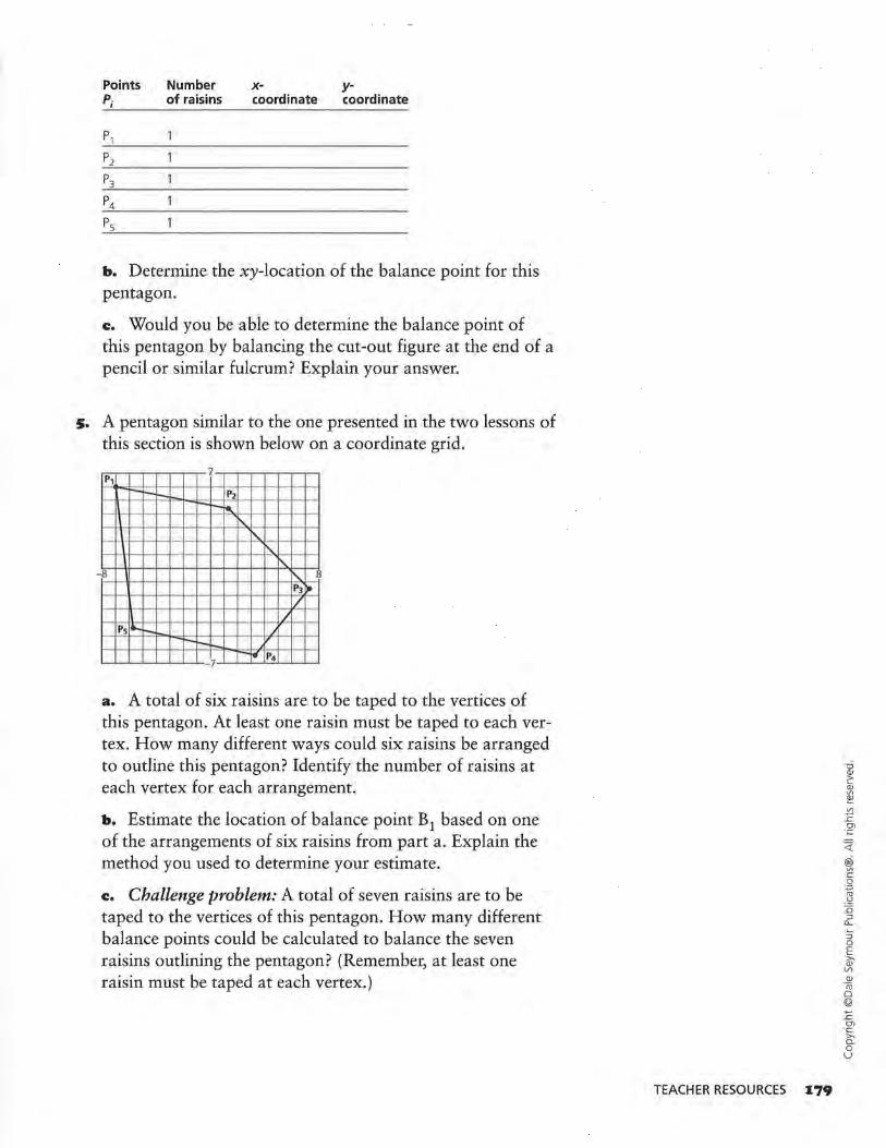
Points Number x- y-P; of raisins coordinate coordinate
b. Determine the xy-location of the balance point for this pentagon.
c. Would you be able to determine the balance point of this pentagon by balancing the cut-out figure at the end of a pencil or similar fulcrum? Explain your answer.
s. A pentagon similar to the one presented in the two lessons of this section is shown below on a coordinate grid.
P1 7 --...... P2
r-r----. ~
~
' -
' -8 r'\.. I P3 )J
I/ I /
Ps *"-r- / ,.__ r-~ l<J P4
7
a. A total of six raisins are to be taped to the vertices of this pentagon. At least one raisin must be taped to each vertex. How many different ways could six raisins be arranged to outline this pentagon? Identify the number of raisins at each vertex for each arrangement.
b. Estimate the location of balance point B1 based on one of the arrangements of six raisins from part a. Explain the method you used to determine your estimate.
c. Challenge problem: A total of seven raisins are to be taped to the vertices of this pentagon. How many different balance points could be calculated to balance the seven raisins outlining the pentagon? (Remember, at least one raisin must be taped at each vertex.)
TEACHER RESOURCES I79
..., ~ CJ)
·~ 0 u
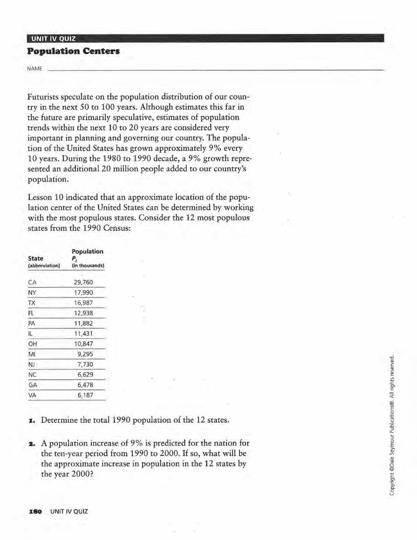
UNIT IV QUIZ
Population Centers
NAME
Futurists speculate on the population distribution of our country in the next 50 to 100 years. Although estimates this far in the future are primarily speculative, estimates of population trends within the next 10 to 20 years are considered very important in planning and governing our country. The population of the United States has grown approximately 9% every 10 years. During the 1980 to 1990 decade, a 9% growth represented an additional 20 million people added to our country's population.
Lesson 10 indicated that an approximate location of the population center of the United States can be determined by working with the most populous states. Consider the 12 most populous states from the 1990 Census:
Population State P; (abbreviation) (in thousands)
CA 29,760
NY 17,990
TX 16,987
FL 12,938
PA 11,882
IL 11,431
OH 10,847
Ml 9,295
NJ 7,730
NC 6,629
GA 6,478
VA 6, 187
I. Determine the total 1990 population of the 12 states.
2. A population increase of 9% is predicted for the nation for the ten-year period from 1990 to 2000. If so, what will be the approximate increase in population in the 12 states by the year 2000?
I80 UNIT IV QUIZ
~
:J 0 E 1U' Vl Q)
(ii 0 @ +-' _c CJ)
-~ c.. 0 u
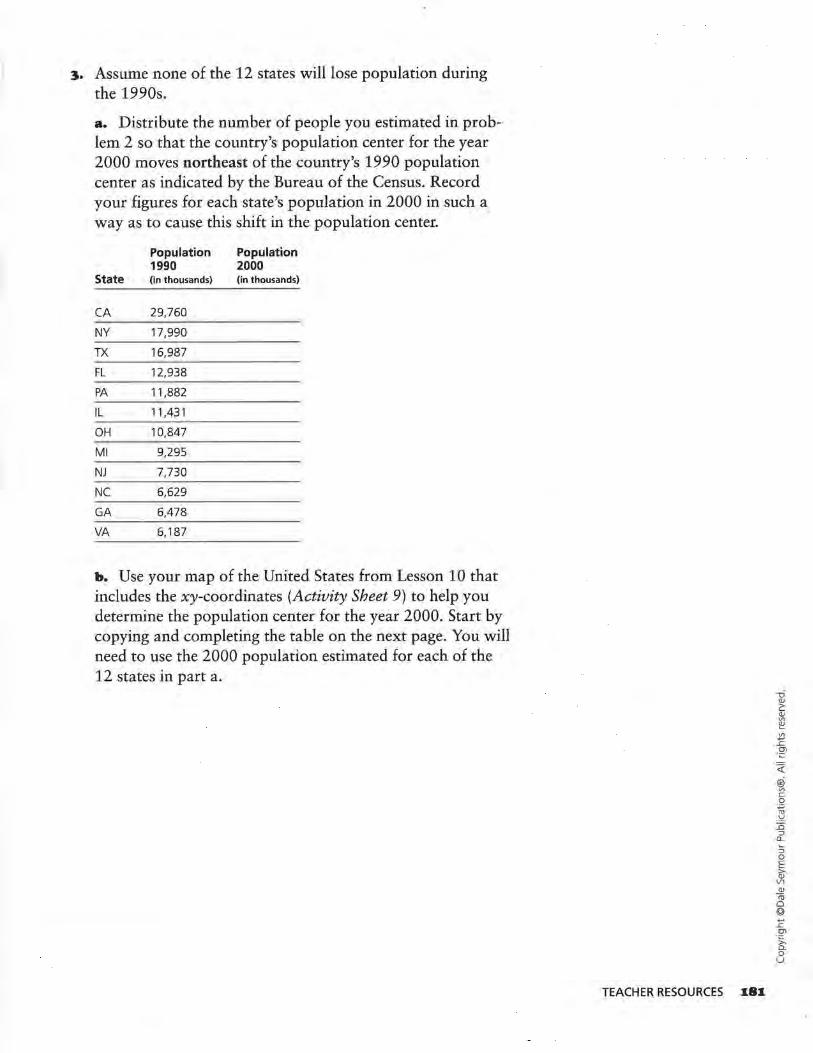
3. Assume none of the 12 states will lose population during the 1990s.
a. Distribute the number of people you estimated in problem 2 so that the country's population center for the year 2000 moves northeast of the country's 1990 population center as indicated by the Bureau of the Census. Record your figures for each state's population in 2000 in such a way as to cause this shift in the population center.
Population Population 1990 2000
State (in thousands) (in thousands)
CA 29,760
NY 17,990
TX 16,987
FL 12,938
PA 11,882
IL 11,431
OH 10,847
Ml 9,295
NJ 7,730
NC 6,629
GA 6,478
VA 6, 187
b. Use your map of the United States from Lesson 10 that includes the xy-coordinates (Activity Sheet 9) to help you determine the population center for the year 2000. Start by copying and completing the table on the next page. You will need to use the 2000 population estimated for each of the 12 states in part a.
TEACHER RESOURCES I8I
<i' @ V\ c 0 ·.;:; ru
·'=' :0 :J
0...
:J 0 E it Vl
<lJ <ti 0 @ +-' ..c
°' -~ 0 u
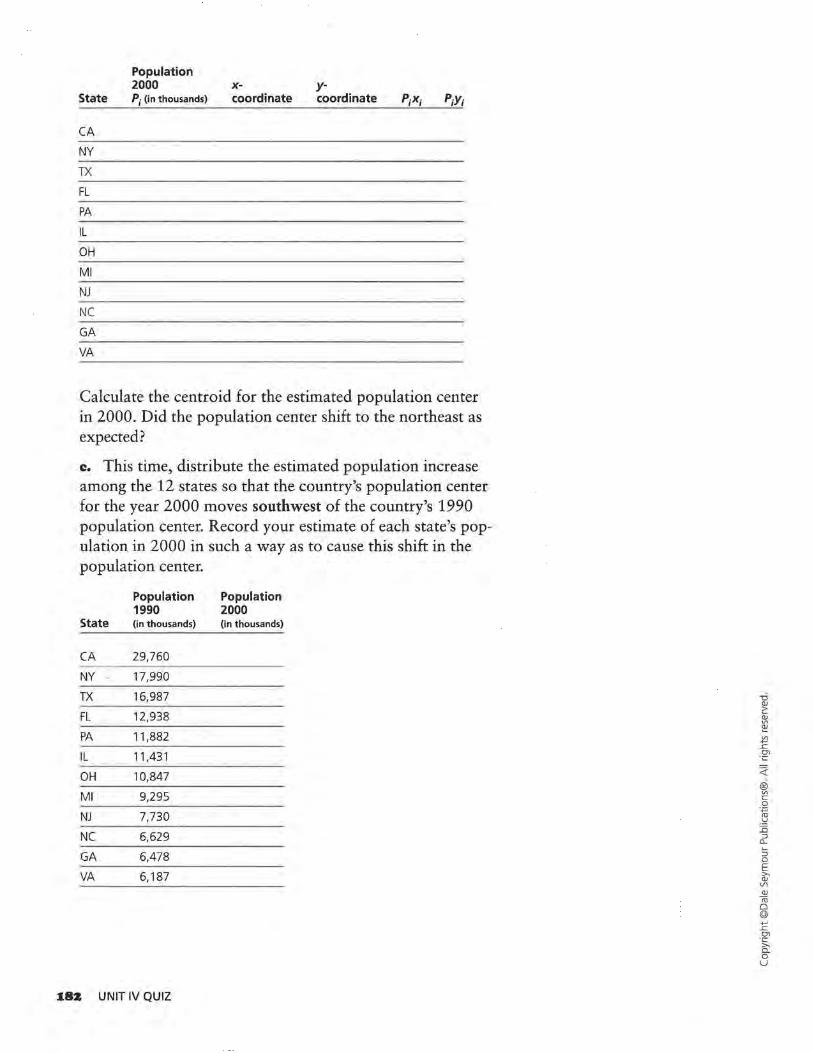
Population 2000 x- y-
State P; (in thousands) coordinate coordinate
CA NY TX FL PA IL OH
Ml
NJ NC GA VA
Calculate the centroid for the estimated population center in 2000. Did the population center shift to the northeast as expected?
c. This time, distribute the estimated population increase among the 12 states so that the country's population center for the year 2000 moves ~outhwest of the country's 1990 population center. Record your estimate of each state's population in 2000 in such a way as to cause this shift in the population center.
Population Population 1990 2000
State (in thousands) (in thousands)
CA 29,760
NY 17,990
TX 16,987
FL 12,938
PA 11,882
IL 11,431
OH 10,847
Ml 9,295
NJ 7,730
NC 6,629
GA 6,478
VA 6, 187
182 UNIT IV QUIZ
-ci "' 2: "' Vl
~ ti _c CJ)
·.:::
<i:'. @i Vl c 0
·.;::; ro -~ ::0 :::J a_
~ 0 E >-"' V)
"' -;;; 0 @ ..., _c CJ)
·~ D.. 0 u
d. Copy and complete the following table to help you determine your estimate for a population shift to the southwest.
Population 2000 x- y-
State P; (in thousands) coordinate coordinate
CA
NY TX FL PA
IL
OH
Ml
NJ
NC
GA VA
Calculate the centroid for your estimated population center in 2000. Did the population center shift to the southwest?
4. Consider your results from problem 3.
a. What conditions might cause a population shift to the northeast?
b. What conditions might cause a population shift to the southwest?
TEACHER RESOURCES X83
UNIT V QUIZ
Minimizing Distances by a Center
NAME
J:. Copy the grid below and consider the four points A, B, C, and D. Locate the center that minimizes the sum of the distances by using helicopter geometry. Label this center as C1.
c
B
D
z. Copy the grid below and consider the three points A, B, and C.
A - ---+---!--- B
(O,O)
a. Locate the center that minimizes the sum of the distances using taxicab geometry. Label this center as C1.
b. Locate the center that minimizes the sum of the distances using helicopter geometry. Label this center as C2•
c. Locate the center that minimizes the greatest distance to any of the points. Label this center as C3"
J:84 UNIT V QUIZ
<(
~ c 0 ·.;:::; re -~ ::i5 ::J
CL
:; 0 E >, Q) VI Q)
ro 0 © +"' ..c O"l -~ D.. 0 u
3. Consider taping a raisin to each of the points A, B, and C in the diagram from problem 2. Determine the center of gravity of the three raisins. Label this point as C4 .
4. Copy the grid below and consider the three points A, B, and C.
c
B
a. Locate the center that minimizes the greatest distance to any of the points. Label this center as C1.
b. Add a fourth point, D, to the diagram such that the center that minimizes the greatest distance to any of the points does not change.
c. Add a fifth point, E, to the diagram such that the center that minimizes the greatest distance to any of the points does change.
TEACHER RESOURCES I8S
<(
@ Vl c 0 ·.;:::;
"' .!.! J5 :::J
0... ~
:::J 0 E (U' Vl QJ
'° 0 @ +"' ..c O"l -~ Cl. 0 u
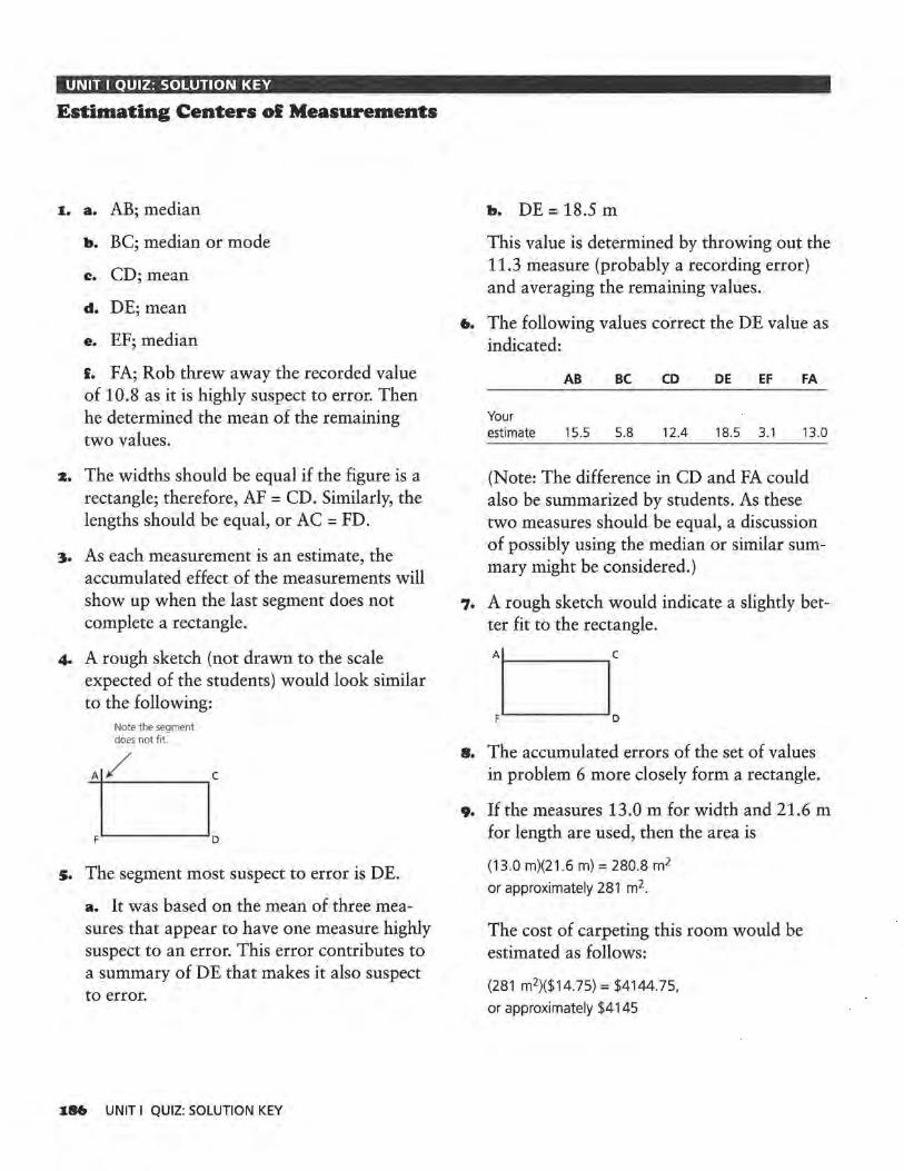
UNIT I QUIZ: SOLUTION KEV
Estimating Centers ol Measurements
I. a. AB; median
b. BC; median or mode
c. CD; mean
d. DE; mean
e. EF; median
f. FA; Rob threw away the recorded value of 10.8 as it is highly suspect to error. Then he determined the mean of the remaining two values.
z. The widths should be equal if the figure is a rectangle; therefore, AF= CD. Similarly, the lengths should be equal, or AC= FD.
3. As each measurement is an estimate, the accumulated effect of the measurements will show up when the last segment does not complete a rectangle.
4. A rough sketch (not drawn to the scale expected of the students) would look similar to the following:
Note the segment does not fit.
~Ai--/ ___ ~C
F D
s. The segment most suspect to error is DE.
a. It was based on the mean of three measures that appear to have one measure highly suspect to an error. This error contributes to a summary of DE that makes it also suspect to error.
I86 UNIT I QUIZ: SOLUTION KEY
b. DE= 18.5 m
This value is determined by throwing out the 11.3 measure (probably a recording error) and averaging the remaining values.
6. The following values correct the DE value as indicated:
AB BC CD DE EF FA
Your estimate 15.5 5.8 12.4 18.5 3.1 13.0
(Note: The difference in CD and FA could also be summarized by students. As these two measures should be equal, a discussion of possibly using the median or similar summary might be considered.)
7. A rough sketch would indicate a slightly better fit to the rectangle.
8. The accumulated errors of the set of values in problem 6 more closely form a rectangle.
9. If the measures 13.0 m for width and 21.6 m for length are used, then the area is
(13.0 m)(21.6 m) = 280.8 m2
or approximately 281 m2.
The cost of carpeting this room would be estimated as follows:
(281 m2)($14.75) = $4144.75,
or approximately $4145
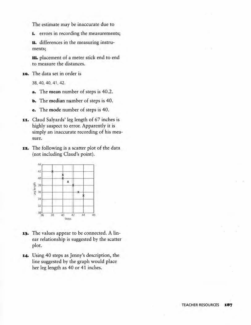
The estimate may be inaccurate due to
i. errors in recording the measurements;
ii. differences in the measuring instruments;
iii. placement of a meter stick end to end . to measure the distances.
10. The data set in order is
38, 40, 40, 41, 42.
a. The mean number of steps is 40.2.
b. The median nvi.mber of steps is 40.
c. The mode number of steps is 40.
11. Claud Salyards' leg length of 67 inches is highly suspect to error. Apparently it is simply an inaccurate recording of his measure.
1z. The following is a scatter plot of the data (not including Claud's point).
44
42
40
-"' x
bi 38 c
.l!I. ~ 36
34
32
38 40 42 44 46 Steps
13. The values appear to be connected. A linear relationship is suggested by the scatter plot.
14. Using 40 steps as Jenny's description, the line suggested by the graph would place her leg length as 40 or 41 inches.
TEACHER RESOURCES 187
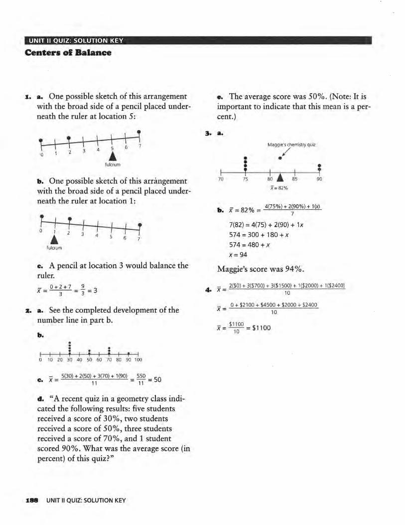
UNIT II QUIZ: SOLUTION KEY
Centers of Balance
1. a. One possible sketch of this arrangement with the broad side of a pencil placed underneath the ruler at location 5:
i I ) -1 ' ) I \ ( 5 6 7
3 4 0 1 2
~ fulcrum
b. One possible sketch of this arrangement with the broad side of a pencil placed underneath the ruler at location 1:
~ I t I ,! I
' I 0 1 2 I I l
~ 3 4 5 6 7
fulcrum
c. A pencil at location 3 would balance the ruler.
x=o+~+7=~=3
z. a. See the completed development of the number line in part b.
b. • • • •
I I • • • I ' I ' I ' I ' I 0 10 20 30 40 so 60 70 80 90 100
X- = 5(30) + 2(50) + 3(70) + 1(90) = 550 = 50
c. 11 11
d. "A recent quiz in a geometry class indicated the following results: five students received a score of 30%, two students received a score of 50%, three students received a score of 70%, and 1 student scored 90%. What was the average score (in percent) of this quiz?"
188 UNIT II QUIZ: SOLUTION KEY
e. The average score was 50%. (Note: It is important to indicate that this mean is a percent.)
3. a.
Maggie's chemistry quiz
/ • • • • • ~ I- I r
70 75 80 ~ 85 90
x=82%
b. X = 82 % = 4(75%) + 2~90%) + 1(x)
7(82) = 4(75) + 2(90) + 1x
574 = 300 + 180 + x 574 = 480 + x X= 94
Maggie's score was 94 % .
- 2($0) + 3($700) + 3($1500) + 1 ($2000) + 1 ($2400) 4. x = 10
0 + $2100 + $4500 + $2000 + $2400 x = ----'-------'-----'-------'---
x = $1100 = $1100 10
10
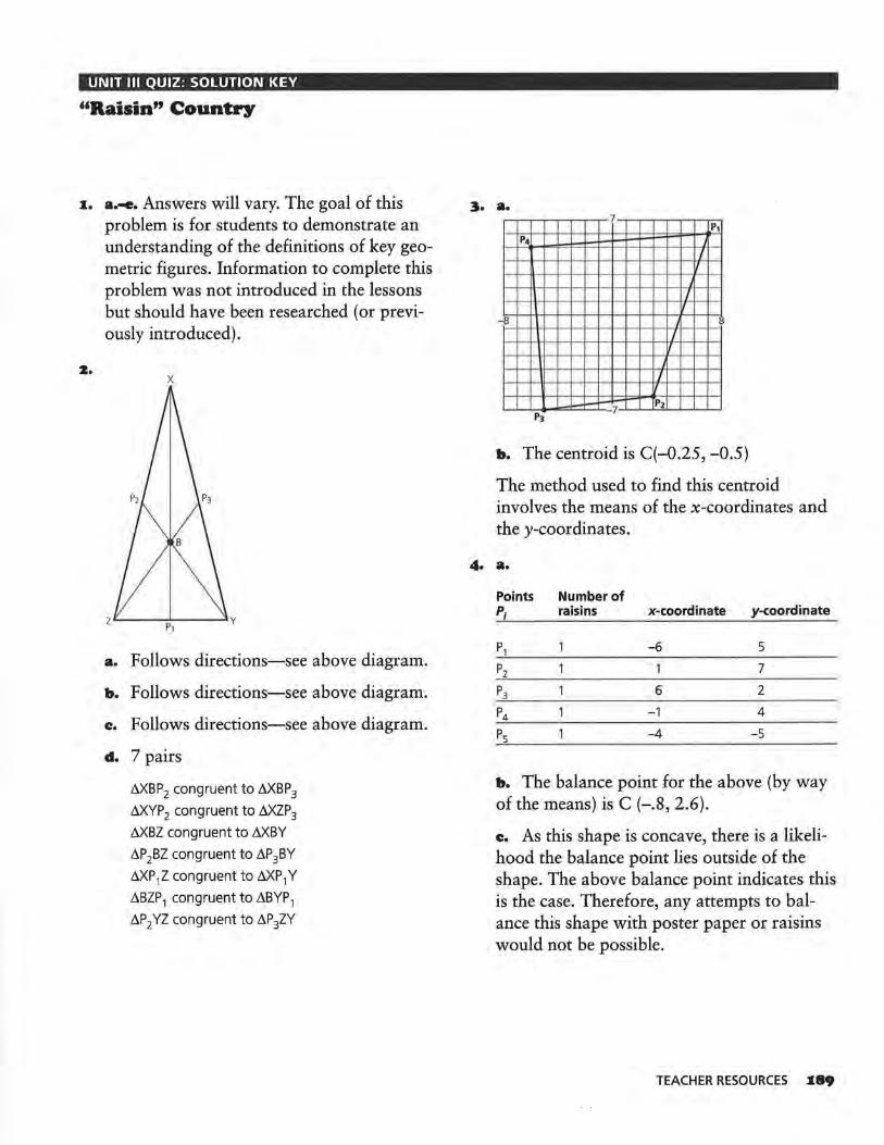
UNIT Ill QUIZ: SOLUTION KEY
"Raisin" Country
I. a.~. Answers will vary. The goal of this problem is for students to demonstrate an understanding of the definitions of key geometric figures. Information to complete this problem was not introduced in the lessons but should have been researched (or previously introduced).
2. x
a. Follows directions-see above diagram.
b. Follows directions-see above diagram.
c. Follows directions-see above diagram.
d. 7 pairs
LiXBP2 congruent to LiXBP3
LiXYP2 congruent to ~P3 LiXBZ congruent to LiXBY
~P2BZ congruent to ~P3BY LiXP1Z congruent to LiXP1 Y
~BZP 1 congruent to ~BYP 1 ~P2 YZ congruent to ~P3ZY
3. a.
4.
7 P1
P4
I
' I
-8 l
I I
I I
7 Pi
b. The centroid is C(-0.25, -0.5)
The method used to find this centroid involves the means of the x-coordinates and they-coordinates.
a.
Points Number of P; raisins x-coordinate y-coordinate
P, -6 5
Pz . 1 7
P3 6 2
P4 -1 4
Ps -4 -5
b. The balance point for the above (by way of the means) is C (-.8, 2.6).
c. As this shape is concave, there is a likelihood the balance point lies outside of the shape. The above balance point indicates this is the case. Therefore, any attempts to balance this shape with poster paper or raisins would not be possible.
TEACHER RESOURCES I89
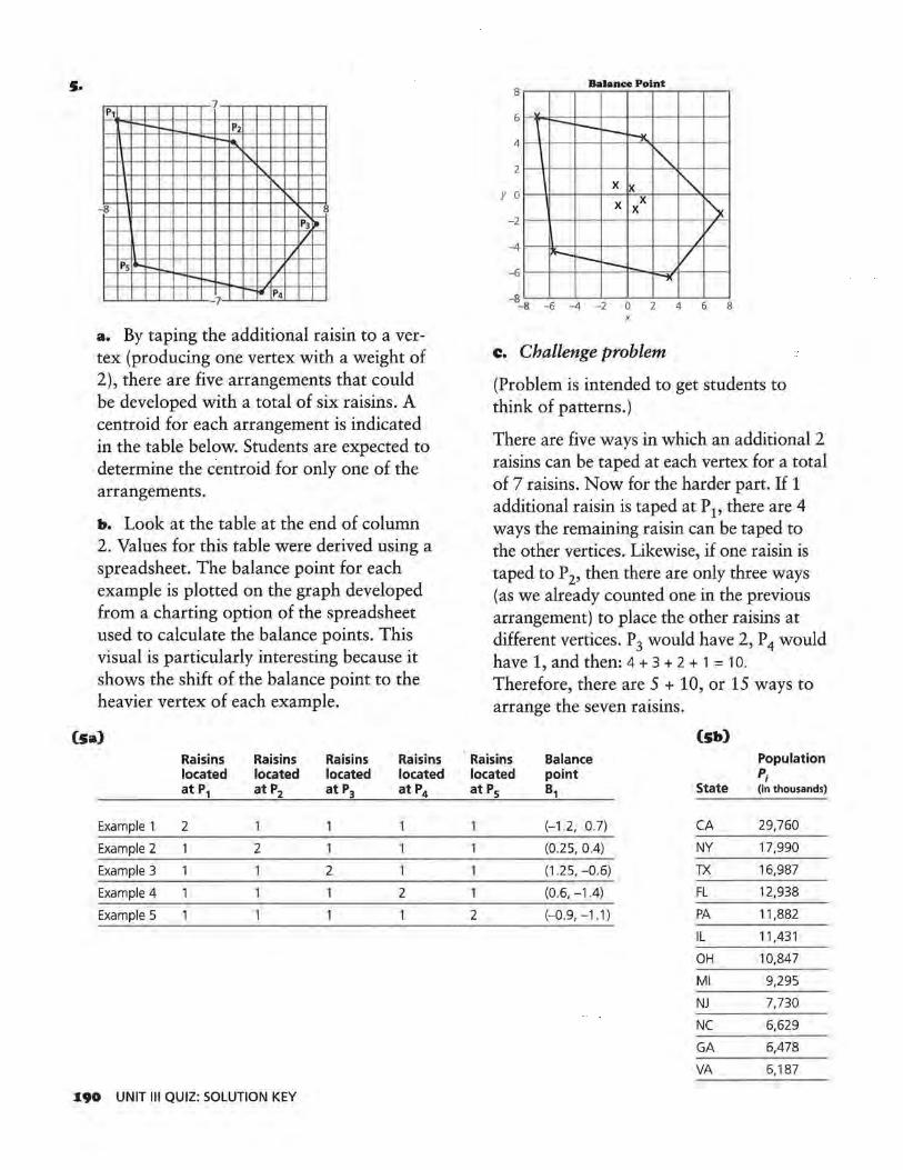
s. P1
7
r-- ..._,_ P2 -"-i.. I !'-
1 ' ' " -8 " P3~ - I/ II .I
Ps i.._ "- J ...... t-. ... ,v IW P4
7
a. By taping the additional raisin to avertex (producing one vertex with a weight of 2), there are five arrangements that could be developed with a total of six raisins. A centroid for each arrangement is indicated in the table below. Students are expected to determine the centroid for only one of the arrangements.
b. Look at the table at the end of column 2. Values for this table were derived using a spreadsheet. The balance point for each
· example is plotted on the graph developed from a charting option of the spreadsheet used to calculate the balance points. This visual is particularly interesting because it shows the shift of the balance point to the heavier vertex of each example.
Csa) Raisins Raisins located located at P1 at P2
Example 1 2 1
Example 2 2
Example 3
Example 4
Example 5
J.90 UNIT Ill QUIZ: SOLUTION KEY
Raisins located at P3
2
1
Raisins located at P4
2
Balance Point 8
6 v ., r--r--t--t-K
\ ~ \ x x ~
x x x r\c .Iv
"'"-,__ v i--
4
2
y 0
-2
-4
-6 1--K
- s-8 -6 -4 -2 0 2 4 6 8 x
c. Challenge problem
(Problem is intended to get students to think of patterns.)
There are five ways in which an additional 2 raisins can be taped at each vertex for a total of 7 raisins. Now for the harder part. If 1 additional raisin is taped at P 1, there are 4 ways the remaining raisin can be taped to the other vertices. Likewise, if one raisin is taped to P 2, then there are only three ways (as we already counted one in the previous arrangement) to place the other raisins at different vertices. P 3 would have 2, P 4 would have 1, and then: 4 + 3 + 2 + 1 = 10.
Therefore, there are 5 + 10, or 15 ways to arrange the seven raisins.
(Sb)
Raisins located at P5
Balance point 81
Population P;
State (in thousands)
(-1.2, 0.7) CA 29,760
(0.25, 0.4) NY 17,990
(1.25, -0.6) TX 16,987
(0.6, -1.4) FL 12,938
2 (-0.9,-1.1) PA 11,882
IL 11,431
OH 10,847
Ml 9,295
NJ 7,730
NC 6,629
GA 6,478
VA 6,187
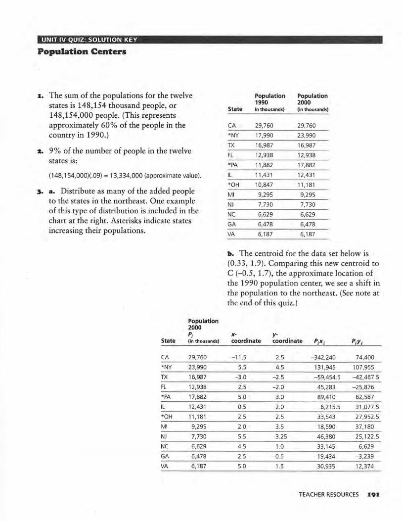
UNIT IV QUIZ: SOLUTION KEY
Population Centers
I. The sum of the populations for the twelve states is 148,154 thousand people, or 148,154,000 people. (This represents approximately 60% of the people in the country in 1990.)
2. 9% of the number of people in the twelve states is:
(148, 154,000)(.09) = 13,334,000 (approximate value).
3. a. Distribute as many of the added people to the states in the northeast. One example of this type of distribution is included in the chart at the right. Asterisks indicate states increasing their populations.
Population 2000 P;
State (in thousands)
CA 29,760
*NY 23,990
TX 16,987
FL 12,938
*PA 17,882
IL 12,431
*OH 11 , 181
Ml 9,295
NJ 7,730
NC 6,629
GA 6,478
VA 6, 187
Population Population 1990 2000
State In thousands) (in thousands)
CA 29,760 29,760
*NY 17,990 23,990
TX 16,987 16,987
FL 12,938 12,938
*PA 11 ,882 17,882
IL 11,431 12,431
*OH 10,847 11, 181
Ml 9,295 9,295
NJ 7,730 7,730
NC 6,629 6,629
GA 6,478 6,478
VA 6,187 6,187
b. The centroid for the data set below is (0.33, 1.9). Comparing this new centroid to C (-0.5, 1.7), the approximate location of the 1990 population center, we see a shift in the population to the northeast. (See note at the end of this quiz.)
x- y-coordinate coordinate P;X; P;Y;
-11.5 2.5 -342,240 74,400
5.5 4.5 131,945 107,955
-3.0 -2 .5 -59,454.5 -42,467.5
2.5 -2 .0 45,283 -25,876
5.0 3.0 89,410 62,587
0.5 2.0 6,215 .5 31,077.5
2.5 2.5 33,543 27,952 .5
2.0 3.5 18,590 37, 180
5.5 3.25 46,380 25, 122.5
4.5 1.0 33, 145 6,629
2.5 -0.5 19,434 -3,239
5.0 1.5 30,935 12,374
TEACHER RESOURCES I9I
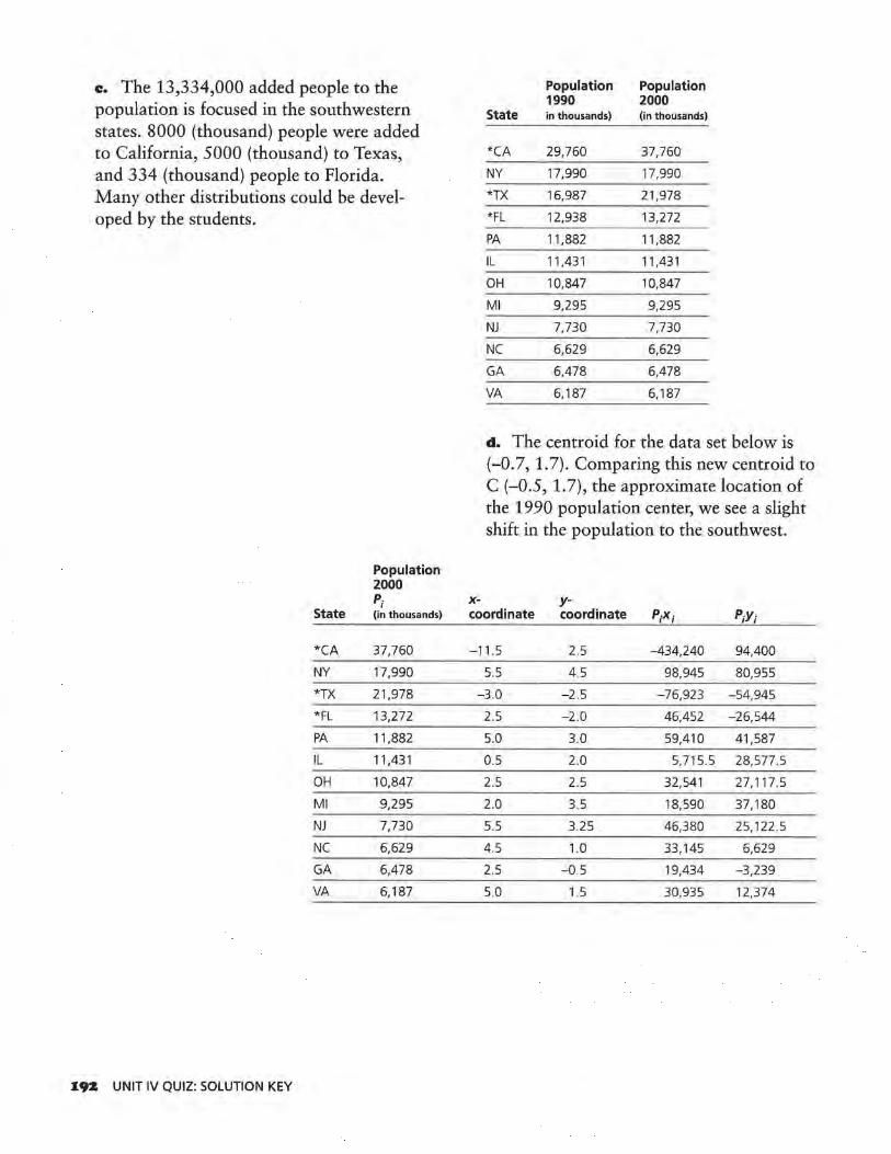
c. The 13,334,000 added people to the population is focused in the southwestern states. 8000 (thousand) people were added to California, 5000 (thousand) to Texas, and 334 (thousand) people to Florida. Many other distributions could be developed by the students.
Population 2000 P;
State (in thousands)
*CA 37,760
NY 17,990
*TX 21,978
*FL 13,272
PA 11,882
IL 11,431
OH 10,847
Ml 9,295
NJ 7,730
NC 6,629
GA 6,478
VA 6, 187
I9Z UNIT IV QUIZ: SOLUTION KEY
x-
Population Population 1990 2000
State in thousands) (in thousands)
*CA 29,760 37,760
NY 17,990 17,990
*TX 16,987 21,978
*FL 12,938 13,272
PA 11,882 11,882
IL 11,431 11,431
OH 10,847 10,847
Ml 9,295 9,295
NJ 7,730 7,730
NC 6,629 6,629
GA 6,478 6,478
VA 6, 187 6,187
d. The centroid for the data set below is (-0.7, 1.7). Comparing this new centroid to C (-0.5, 1.7), the approximate location of the 1990 population center, we see a slight shift in the population to the southwest.
y-coordinate coordinate P;X; P;Y;
-11.5 2.5 -434,240 94,400
5.5 4.5 98,945 80,955
-3.0 -2.5 -76,923 -54,945
2.5 -2.0 46,452 -26,544
5.0 3.0 59,410 41,587
0.5 2.0 5,715.5 28,577.5
2.5 2.5 32,541 27, 117.5
2.0 3.5 18,590 37,180
5.5 3.25 46,380 25,122.5
4.5 1.0 33,145 6,629
2.5 -0.5 19,434 -3,239
5.0 1.5 30,935 12,374
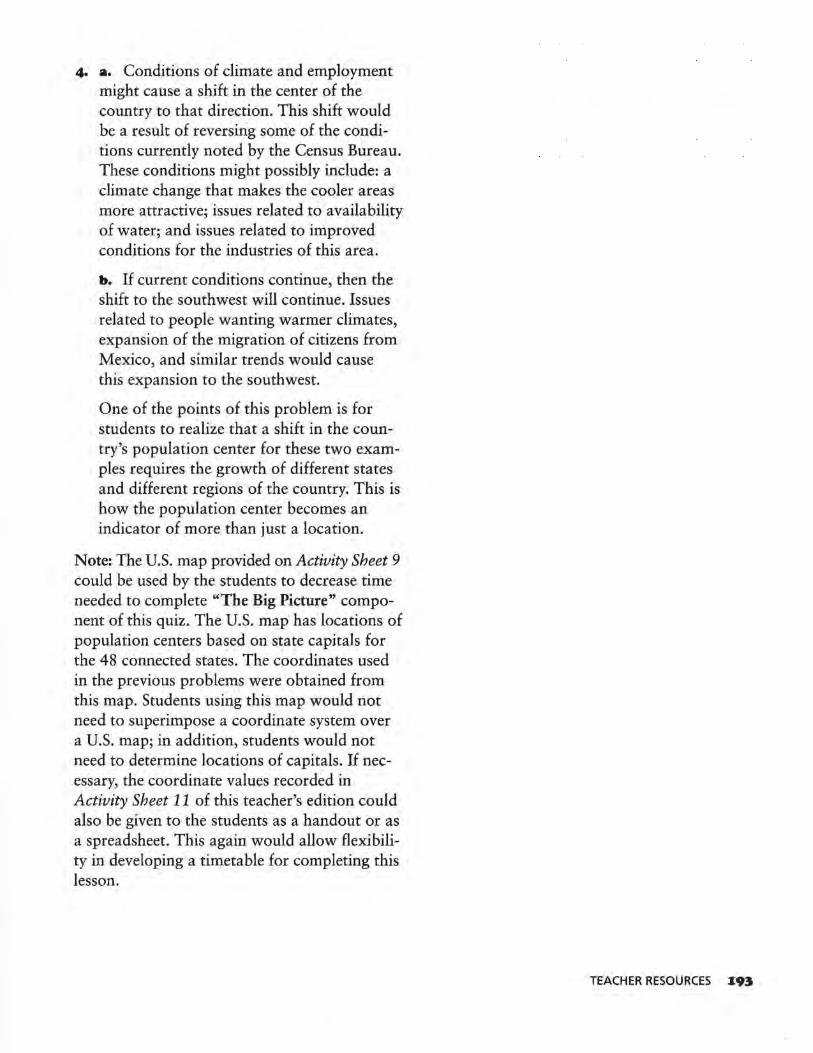
4. a. Conditions of climate and employment might cause a shift in the center of the country to that direction. This shift would be a result of reversing some of the conditions currently noted by the Census Bureau. These conditions might possibly include: a climate change that makes the cooler areas more attractive; issues related to availability of water; and issues related to improved conditions for the industries of this area.
b. If current conditions continue, then the shift to the southwest will continue. Issues related to people wanting warmer climates, expansion of the migration of citizens from Mexico, and similar trends would cause this expansion to the southwest.
One of the points of this problem is for students to realize that a shift in the country's population center for these two examples requires the growth of different states and different regions of the country. This is how the population center becomes an indicator of more than just a location.
Note: The U.S. map provided on Activity Sheet 9 could be used by the students to decrease time needed to complete "The Big Picture" component of this quiz. The U.S. map has locations of population centers based on state capitals for the 48 connected states. The coordinates used in the previous problems were obtained from this map. Students using this map would not need to superimpose a coordinate system over a U.S. map; in addition, students would not need to determine locations of capitals. If necessary, the coordinate values recorded in Activity Sheet 11 of this teacher's edition could also be given to the students as a handout or as a spreadsheet. This again would allow flexibility in developing a timetable for completing this lesson.
TEACHER RESOURCES I93
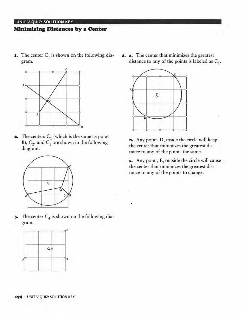
UNIT V QUIZ: SOLUTION KEY
Minimizing Distances by a Center
I. The center cl is shown on the following diagram.
c
z. The centers C1 (which is the same as point B), C2, and C3 are shown in the following diagram.
3. The center C4 is shown on the following diagram.
A B
I94 UNIT V QUIZ: SOLUTION KEY
4. a. The center that minimizes the greatest distance to any of the points is labeled as C1.
0
C1
b. Any point, D, inside the circle will keep the center that minimizes the greatest distance to any of the points the same.
c:. Any point, E, outside the circle will cause the center that minimizes the greatest distance to any of the points to change.
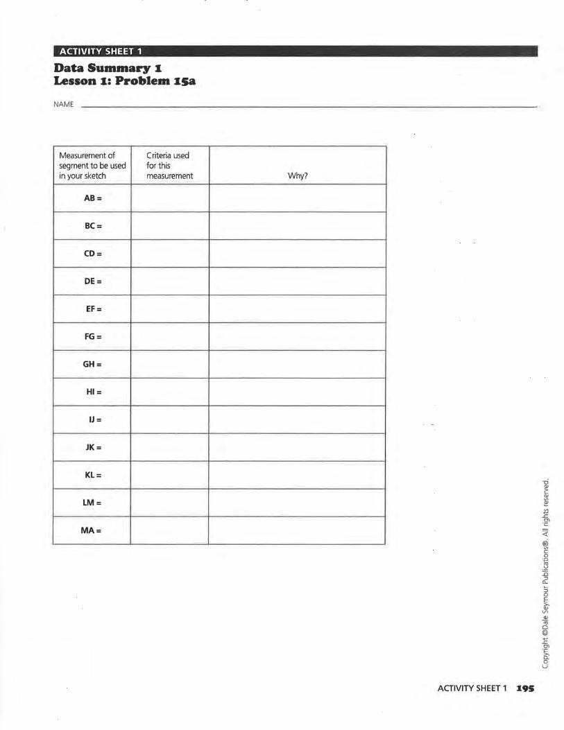
ACTIVITY SHEET 1
Data Summary • Lesson •: Problem •sa NAME
Measurement of Criteria used segment to be used for this in your sketch measurement
AB=
BC=
CD=
DE=
Ef=
FG=
GH=
HI=
IJ =
JK=
KL=
LM=
MA=
Why?
ACTIVITY SHEET 1 I9S
<(
@ V1 c 0
·.;:;
. ~ :0 :J
CL
OJ 0 E ~
V1 (lJ
(ij 0 @ +-' .<::: en
·~ 0. 0 u
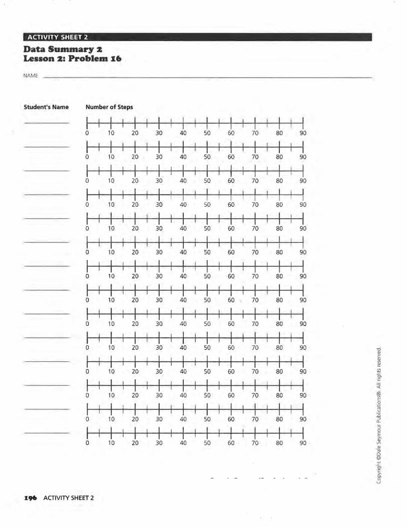
ACTIVITY SHEET 2
Data Summary z Lesson z: Problem I6
NAME------- - ---------------
Student's Name Number of Steps
I I I I I I I I I 0 10 20 30 40 50 60 70 80 90
I I I I I I I 0 10 20 30 40 50 60 70 80 90
I I I I I I I I I 0 10 20 30 40 50 60 70 80 90
I I I I I I I I 0 10 20 30 40 50 60 70 80 90
I I I I I I I I 0 10 20 30 40 50 60 70 80 90
I I I I I I I I I I 0 10 20 30 40 50 60 70 80 90
I I I I I I I I I I 0 10 20 30 40 50 60 70 80 90
I I I I I I I I I 0 10 20 30 40 50 60 ' 70 80 90
I I I I I I I I I 0 10 20 30 40 50 60 70 80 90
I I I I I I I I I 0 10 20 30 40 50 60 70 80 90
I I 0 10 20 30 40 50 60 70 80 90
I I I I 0 10 20 30 40 50 60 70 80 90
I I I I I 0 10 20 30 40 50 60 70 80 90
I I I I 0 10 20 30 40 50 60 70 80 90
I96 ACTIVITY SHEET 2
-ci <lJ c. <lJ VI
~ ~ .s::: 0\ ·c
<l: @i VI c 0
·.;:::; re
-~ ::c :::J
0...
::; 0 E ;., <lJ Vl <lJ m 0 © +-' .s::: -~ >. a. 0 u
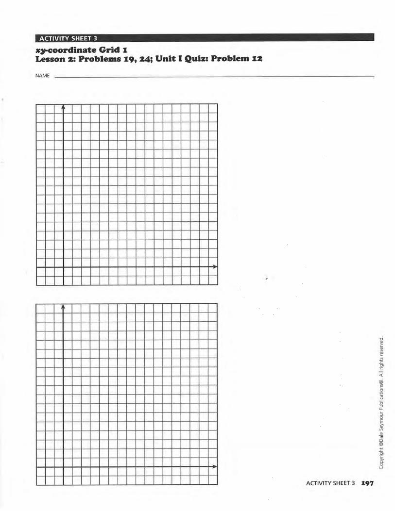
ACTIVITY SHEET 3
*~coordinate Grid 1 Lesson z: Problems 19, 24; Unit I Quiz: Problem 12
NAME
,,
'
--
,
ACTIVITY SHEET 3 197
<(
@i Vl c 0
·.;:::; ro
-'=' :n ::::l a_
::::l 0 E iLJ' Vl
<lJ -ru 0 @ +-' £ O"l ·~ o._ 0 u
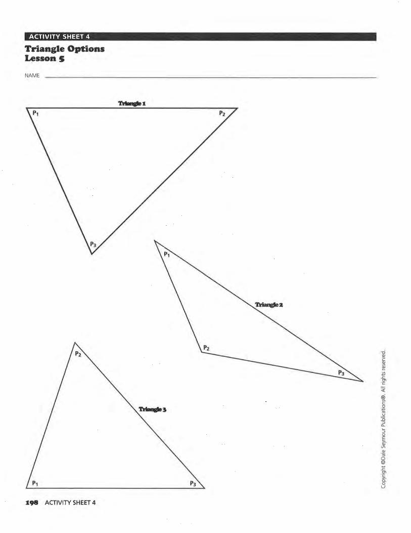
ACTIVITY SHEET 4
Triangle Options Lesson S
NAME
I98 ACTIVITY SHEET 4
<! ® V> c 0 ·.;::; l1l -~ 15 :J c... ~
:J 0 E iU' VI QJ
(ij 0 © ..., ..c
°' ·c >. 0. 0 u
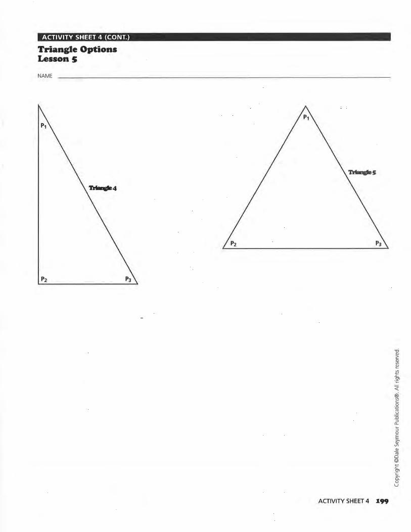
ACTIVITY SHEET 4 (CONT.)
Triangle Options Lesson S
NAME
ACTIVITY SHEET 4 I99
<i: @ V1 c 0 ·.;:::; ru -~ JS :J
0...
:J 0 E iii' VI Q)
(ij 0 @ +-' .r::: O'l
· ;:::: » a. 0 u
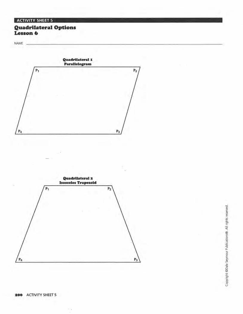
ACTIVITY SHEET 5
Quadrilateral Options Lesson 6
NAME
ZOO ACTIVITY SHEET 5
Quadrilateral J: ParalleloP"am
Quadrilateral z Isosceles Trapezoid
-d Cl.I 2: Cl.I V\
1!! .l!l ..c °' ·.:::
<(
@) V\ c 0
·~
"' -~ ::c :::J
a... ::; 0 E ~
VI (lJ
Iii 0 @ .... ..c °' ·~ 0.. 0 u
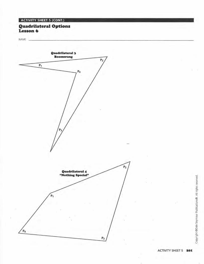
ACTIVITY SHEET 5 (CONT.)
Quadrilateral Options Lesson 6
NAME
Quadrilateral :J Boomerang
ACTIVITY SHEET 5 Z01
~ @ V\ c 0
·.;::; rn
.'=! ::0
:::> a..
:::> 0 E >. QJ VI QJ
-;;; 0 @ +' ..c Ol ·~ 0.. 0 u
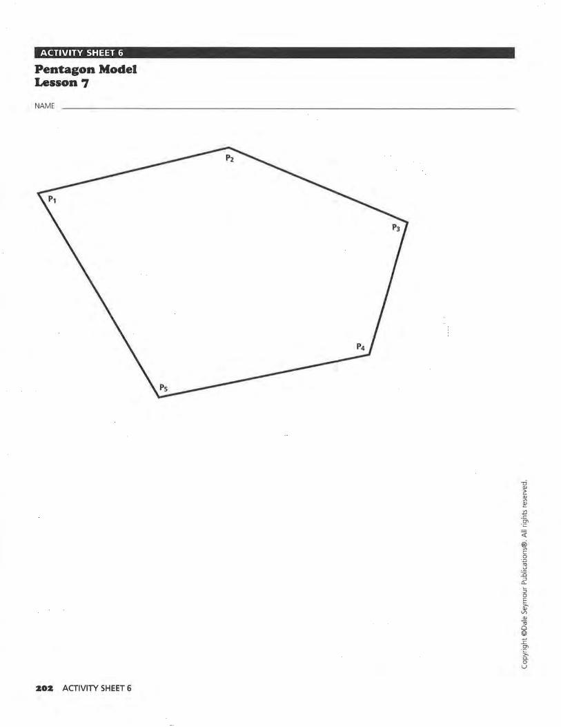
ACTIVITY SHEET 6
Pentagon Model Lesson 7
NAME
:&O:& ACTIVITY SHEET 6
<(
® Vl c 0
·.;::;
-~ :0
:::J CL
:::J 0 E >OJ
V>
OJ rn 0 © +-' ..c Ol -~ 0. 0 u
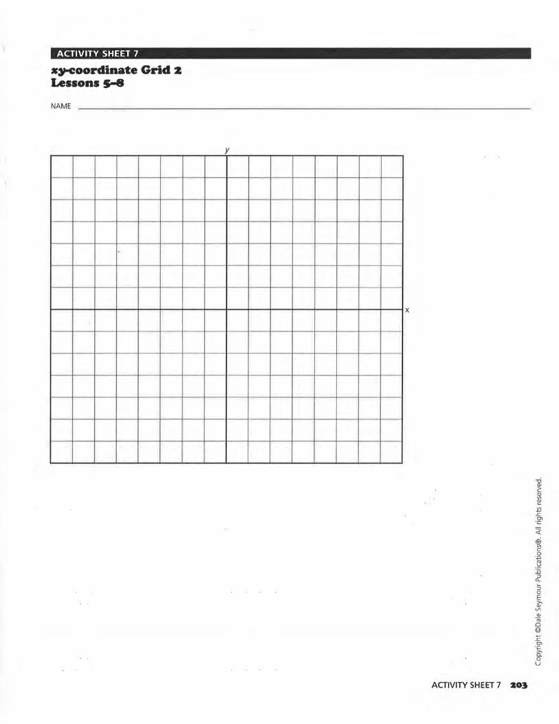
ACTIVITY SHEET 7
*~oorclinate Grid z Lessons 5-8
NAME
y
ACTIVITY SHEET 7 Z03
<i' ® Vl c 0
·.;:::;
"' -~ J5 :J "-~
:J 0 E 5J' Vl Q)
-ro 0 @ +-' _c Ol
· ;:::: » a. 0 u
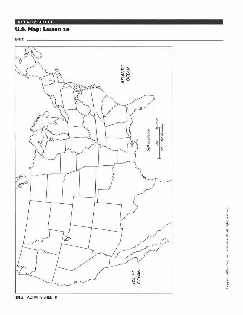
ACTIVITY SHEET 8
U.S. Map: Lesson 10
NAME
V>
..!!! .E 0 !:! 0 ;!l
-~ '<!" <11
E .2
1i'l :;;
~ 0 0 ..... 0 '<!"
0 0
~ N
0 0 \.'.) N
0
-0 CV 2: CV Vl
~ .l!l ..c 01 ·c
<(
@ Vl c 0 ·.;:::; <ll
.!d ::ci :::J
c... :; 0 E :>, CV
V> CV
u (ij
< 0
li:: ~ @
0 ..., ..c
~ u 01
0 ·~ o._ 0 u
Z04 ACTIVITY SHEET 8
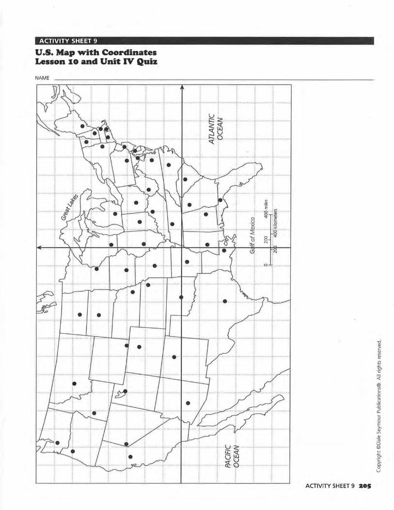
ACTIVITY SHEET 9
U.S. Map with Coordinates Lesson IO and Unit IV Quiz
NAME
... , ............ , ........................ , .................... .. l ............ \ ........... t .......... .
••••••••••••loo"'•
.. ~ .
.. ...... y ........ t·· ....... + ...................... , .. _.~ ~ ......... f ........ .. : : : ; ::s u :
. ....... ···~ ........... .
i .. ..... + ......... .. f"""''"'l'"""''''' ........... + .... ~ .. .p,_ .. -+·· ...... .. ...... '''!" ....... .
. . . ' • o • ~ ' ' ' • ' o + o o • o 'z o ' o o o o o ' o ' o :• o ' • o ' ' ' ' o o ' • o o o o ' ' ' o o o • ' I ' • o o o • '
l j .... ~ .. .. .... t ........ • ~---'-...--'L..--t----t
........ .............. ..
; ~ ~
L. ... ~ ... i ~ .... ~ ;a;
.§ : ~ . :><; ~ ··j· ........ ~ ......... ·io ........ . . '-!-.; 0 .~ : 0 0 : • ~ N
;_...--,..(f--t...._'T""' 1 •
. . . .. . ·:·.. .. . . . . . . :· . . . . . . . . . . . . . . ..... ~.. . . . . . . ·:. . ...... '.
: . : . ........ -~ .... ······-r····· ... , - ~·· .....
OUOl>oO•OO:OO I Oooooo70000000oo o :<o o oOO ooo
. . . '' •••••• "''''"'''''f''h•I •• •• ••;•••• ''''''":' ''' •••••• •• •••••• '''''' '''''"' '
,-;;:--7=1-.-._;_,_ .. ;...:.;.. .. .. ......... .. i ............ i ............ ! .......... .
..... ............... l ...... .. ........... ~ ............ : ............ ; ........... .
' . . . . . . . ···-r·········-·T···-·······r···········~-.
....... j ............ ; .
l :
.... 1..;;i .• ~ ........ i ............ ; ........ _., u:- : : N Qi : : ....., \<..) . .
.... ~·0 ·· ....... ; ............ 1 ........... .
ACTIVITY SHEET 9 20S
<!'. ® Vl c 0
·.;::;
.~ ::0 ::i
CL
::i 0 E >, Q) l/)
Q)
~ @ +-' £ Ol -~ 0. 0 u
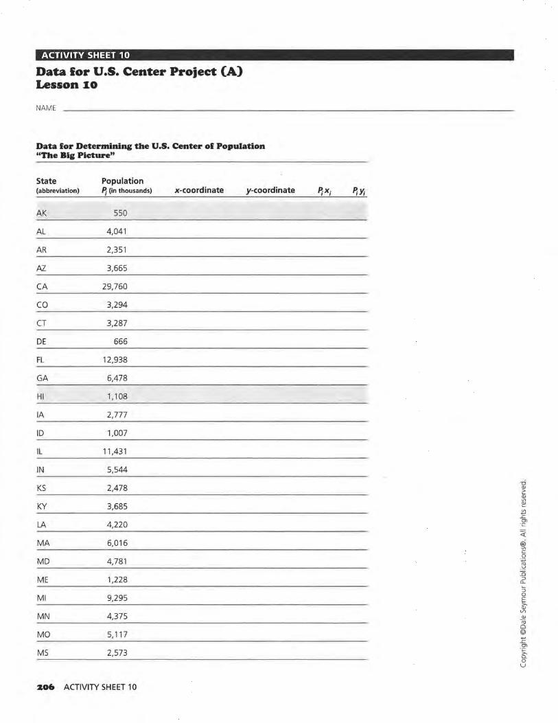
ACTIVITY SHEET 10
Data for U.S. Center Project (A) Lesson IO
NAME
Data for Determining the U.S. Center of Population "The Big Picture"
State Population (abbreviation) P; (in thousands) x-coordinate y-coordinate
AK 550
AL 4,041
AR 2,351
AZ 3,665
CA 29,760
co 3,294
CT 3,287
DE 666
FL 12,938
GA 6,478
HI 1, 108
IA 2,777
ID 1,007
IL 11,431
IN 5,544
KS 2,478
KY 3,685
LA 4,220
MA 6,016
MD 4,781
ME 1,228
Ml 9,295
MN 4,375
MO 5, 117
MS 2,573
Z06 ACTIVITY SHEET 10
P;x; P; Yi
<(
@5 Vl c 0 ·.;:; n; -~ :0 :J "-::; 0 E >, CIJ Vl
CIJ "iii 0 @ +-' ..c
°' ·.: >, o_ 0 u
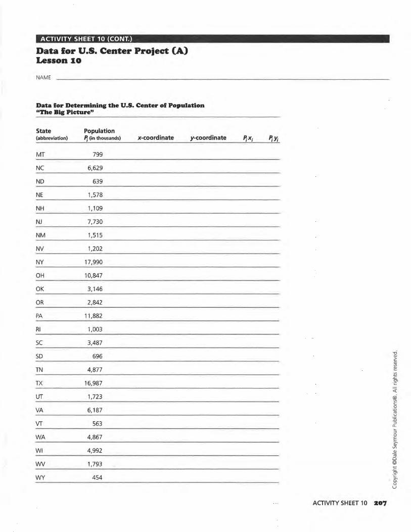
ACTIVITY SHEET 10 (CONT.)
Data for U.S. Center Project (A) Lesson 10
NAME
Data for Determining the U.S. Center of Population "The Big Picture"
State Population (abbreviation) P; (in thousands) x-coordinate y-coordinate
MT 799
NC 6,629
ND 639
NE 1,578
NH 1, 109
NJ 7,730
NM 1,515
NV 1,202
NY 17,990
OH 10,847
OK 3,146
OR 2,842
PA 11,882
RI 1,003
SC 3,487
SD 696
TN 4,877
TX 16,987
UT 1,723
VA 6, 187
VT 563
WA 4,867
WI 4,992
WV 1,793
WY 454
P;x; P; Y;
ACTIVITY SHEET 10 Z07
<i'. ® Vl c 0 -~
ro -~ ::0
:::J "-:::J 0 E ii? VI QI
~ 0 @ +-' _c 01 -~ Q_ 0 u
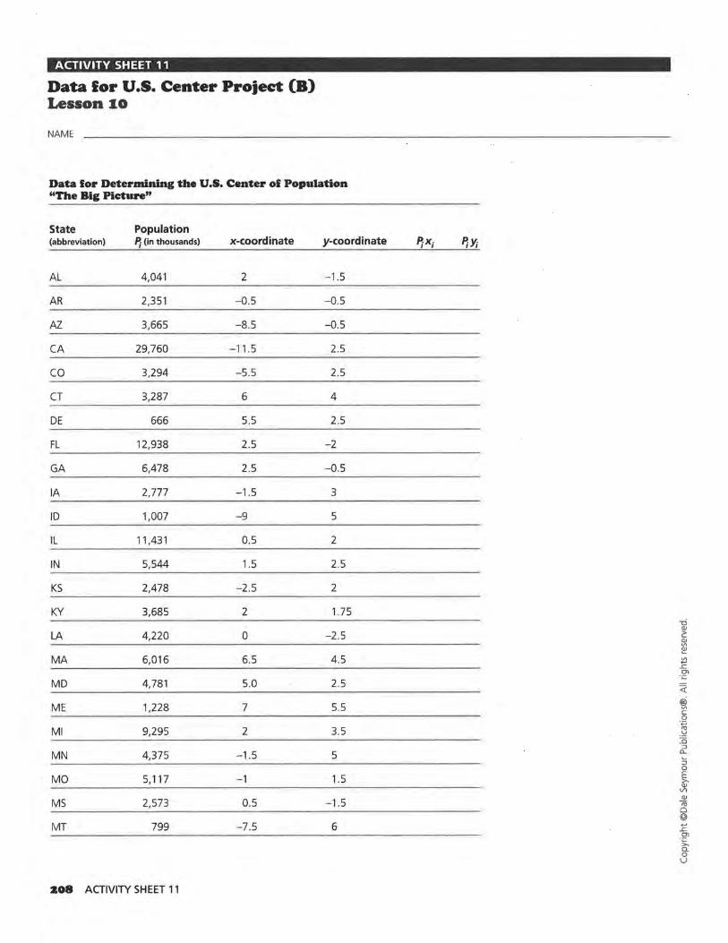
ACTIVITY SHEET 11
Data lor U.S. Center Project (B) Lesson •o
NAM E
Data for Determining the U.S. Center of Population "The Big Picture"
State Population (abbreviation) P; (in thousands) x-coordinate y-coordinate
AL 4,041 2 -1.5
AR 2,351 - 0.5 -0.5
AZ 3,665 -8.5 -0.5
CA 29,760 -1 1.5 2.5
co 3,294 -5.5 2.5
CT 3,287 6 4
DE 666 5.5 2.5
FL 12,938 2.5 -2
GA 6,478 2.5 -0.5
IA 2,777 -1 .5 3
ID 1,007 -9 5
IL 11,431 0.5 2
IN 5,544 1.5 2.5
KS 2,478 -2 .5 2
KY 3,685 2 1.75
LA 4,220 0 - 2.5
MA 6,016 6.5 4.5
MD 4,781 5.0 2.5
ME 1,228 7 5.5
Ml 9,295 2 3.5
MN 4,375 -1.5 5
MO 5, 117 -1 1.5
MS 2,573 0.5 -1 .5
MT 799 -7.5 6
Z08 ACTIVITY SHEET 11
P;x; P;Y;
-0 QJ
c QJ Vl e: ~ ..c Ol
·;:::
~
® Vl c 0 ·.;::;
"' .;e ::0 ::>
a._
::; 0 E >, QJ Vl QJ
Iii Cl @ ..... ..c Ol ·~
a. 0 u
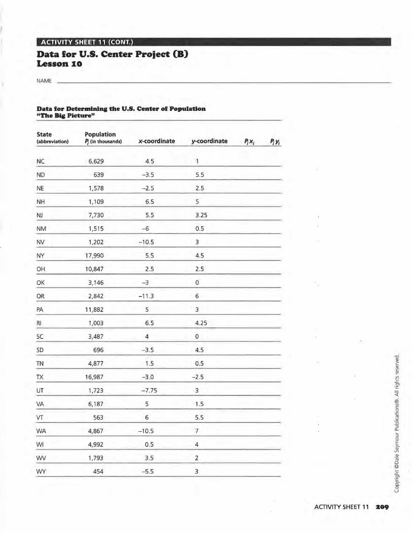
ACTIVITY SHEET 11 (CONT.)
Data lor U.S. Center Project (B) Lesson IO
NAME
Data for Determining the U.S. Center of Population "The Bia Picture"
State Population (abbreviation) P; (in thousands) x-coordinate y-coordinate
NC 6,629 4.5
ND 639 -3.5 5.5
NE 1,578 -2.5 2.5
NH 1, 109 6.5 5
NJ 7,730 5.5 3.25
NM 1,515 -6 0.5
NV 1,202 -10.5 3
NY 17,990 5.5 4.5
OH 10,847 2.5 2.5
OK 3, 146 -3 0
OR 2,842 -11.3 6
PA 11,882 5 3
RI 1,003 6.5 4 .25
SC 3,487 4 0
SD 696 -3.5 4.5
TN 4,877 1.5 0.5
TX 16,987 -3 .0 -2.5
UT 1,723 -7.75 3
VA 6,187 5 1.5
VT 563 6 5.5
WA 4,867 -10.5 7
WI 4,992 0.5 4
WV 1,793 3.5 2
WY 454 -5.5 3
P;x; P;Y;
-0 Cli c: Cli Vl
~ ~ ..c 0\
· ;::::
<(
® Vl c 0 ·.;:::; ro
.!=! ::0 :J "-:; 0 E >. Cli Vl Cli n; 0 © ..., ..c 0\
·;:::: >. c. 0 u
ACTIVITY SHEET 11 209
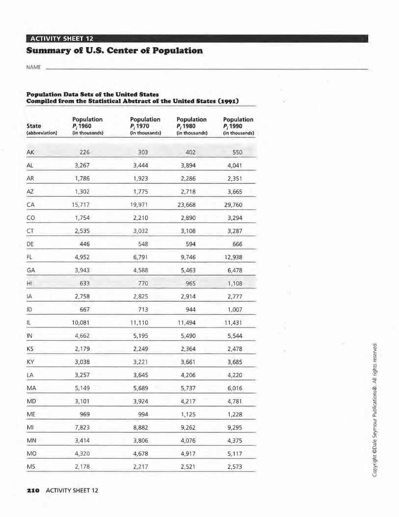
ACTIVITY SHEET 12
Summary ol U.S. Center ol Population
NAME
Population Data Sets of the United States Compiled from the Statistical Ahstraet of the United States (I991)
Population Population Population Population State P; 1960 P; 1970 P; 1980 P; 1990 (abbreviation) (in thousands) (in thousands) (in thousands) (in thousands)
AK 226 303 402 550
AL 3,267 3,444 3,894 4,041
AR 1,786 1,923 2,286 2,351
AZ 1,302 1,775 2,718 3,665
CA 15,717 19,971 23,668 29,760
co 1,754 2,210 2,890 3,294
CT 2,535 3,032 3,108 3,287
DE 446 548 594 666
FL 4,952 6,791 9,746 12,938
GA 3,943 4,588 5,463 6,478
HI 633 770 965 1, 108
IA 2,758 2,825 2,914 2,777
ID 667 713 944 1,007
IL 10,081 11,110 11,494 11,431
IN 4,662 5, 195 5,490 5,544 -0
KS 2, 179 2,249 2,364 2,478 <lJ ~ <lJ .,,
KY 3,038 3,221 3,661 3,685 e:! .,, +-' ..c
LA 3,257 3,645 4,206 4,220 0\
·c
<(
MA 5, 149 5,689 5,737 6,016 @i .,, c 0
MD 3,101 3,924 4,217 4,781 ·;:;
"' .~ ]5
ME 969 994 1, 125 1,228 :J 0...
:; Ml 7,823 8,882 9,262 9,295
0 E >-<lJ VI
MN 3,414 3,806 4,076 4,375 <lJ <ii 0
MO 4,320 4,678 4,917 5, 117 @ +-' ..c 0\
MS 2,178 2,217 2,521 2,573 ·c >-o_ 0 u
ZIO ACTIVITY SHEET 12
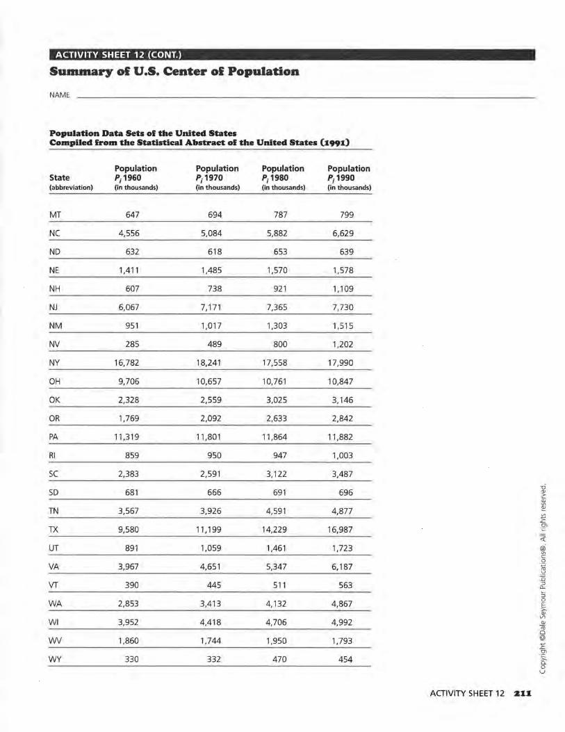
ACTIVITY SHEET 12 (CONT.)
Summary ol U.S. Center ol Population
NAME
Population Data Sets of the United States Compiled from the Statistical Abstract of the United States b99d
Population Population Population Population State P; 1960 P; 1970 P; 1980 P; 1990 (abbreviation) (in thousands) (in thousands) (in thousands) (in thousands)
MT 647 694 787 799
NC 4,556 5,084 5,882 6,629
ND 632 618 653 639
NE 1,411 1,485 1,570 1,578
NH 607 738 921 1, 109
NJ 6,067 7, 171 7,365 7,730
NM 951 1,017 1,303 1,515
NV 285 489 800 1,202
NY 16,782 18,241 17,558 17,990
OH 9,706 10,657 10,761 10,847
OK 2,328 2,559 3,025 3, 146
OR 1,769 2,092 2,633 2,842
PA 11,319 11,801 11,864 11,882
RI 859 950 947 1,003
SC 2,383 2,591 3, 122 3,487
-0 SD 681 666 691 696 QJ
2: QJ V\
TN 3,567 3,926 4,591 4,877 ~ ~ ..c
TX 9,580 11, 199 14,229 16,987 0\ -.::::
<{
UT 891 1,059 1,461 1,723 @i Vl c 0
VA 3,967 4,651 5,347 6,187 -_;::; rn -~ J5
VT 390 445 511 563 ::J CL
::; WA 2,853 3,413 4,132 4,867
0 E >-, QJ VI
WI 3,952 4,418 4,706 4,992 QJ
--ro 0
WV 1,860 1,744 1,950 1,793 @ +-' ..c 0\
WY 330 332 470 454 -.:::: >-, Q_
0 u
ACTIVITY SHEET 12 2II
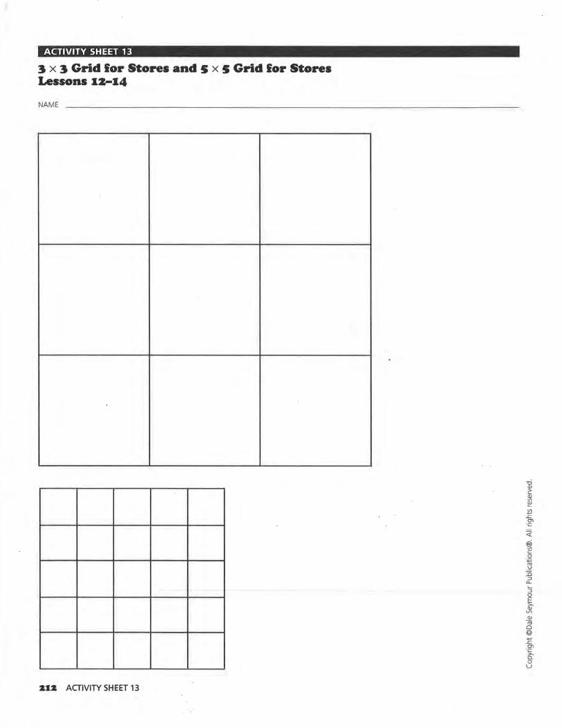
ACTIVITY SHEET 13
3 x 3 Grid lor Stores and s x s Grid lor Stores Lessons IZ-I4
NAME
ZIZ ACTIVITY SHEET 13
<(
@i Vl c 0 -.;::;
"' _!,,! J5 :J
C>-
:; 0 E >, QJ Vl QJ
-;;; 0 © +-' __c
°' -~ 0 u
9 781572 322363
ISBN 1-57232-236-5