This article was downloaded by: [University of California Davis]On: 02 August 2011, At: 11:27Publisher: Taylor & FrancisInforma Ltd Registered in England and Wales Registered Number: 1072954 Registered office: Mortimer House,37-41 Mortimer Street, London W1T 3JH, UK

Transactions of the American Fisheries SocietyPublication details, including instructions for authors and subscription information:http://www.tandfonline.com/loi/utaf20

Falling Behind: Delayed Growth Explains Life-HistoryVariation in Snake River Fall Chinook SalmonT. Alex Perkins a b & Henrïette I. Jager ba Center for Population Biology, University of California at Davis, One Shields Avenue, Davis,California, 95616, USAb Oak Ridge National Laboratory, Environmental Sciences Division, Post Office Box 2008, OakRidge, Tennessee, 37831-6038, USA

Available online: 02 Aug 2011

To cite this article: T. Alex Perkins & Henrïette I. Jager (2011): Falling Behind: Delayed Growth Explains Life-History Variationin Snake River Fall Chinook Salmon, Transactions of the American Fisheries Society, 140:4, 959-972

To link to this article: http://dx.doi.org/10.1080/00028487.2011.599257

PLEASE SCROLL DOWN FOR ARTICLE

Full terms and conditions of use: http://www.tandfonline.com/page/terms-and-conditions

This article may be used for research, teaching and private study purposes. Any substantial or systematicreproduction, re-distribution, re-selling, loan, sub-licensing, systematic supply or distribution in any form toanyone is expressly forbidden.

The publisher does not give any warranty express or implied or make any representation that the contentswill be complete or accurate or up to date. The accuracy of any instructions, formulae and drug doses shouldbe independently verified with primary sources. The publisher shall not be liable for any loss, actions, claims,proceedings, demand or costs or damages whatsoever or howsoever caused arising directly or indirectly inconnection with or arising out of the use of this material.

Transactions of the American Fisheries Society 140:959–972, 2011American Fisheries Society 2011ISSN: 0002-8487 print / 1548-8659 onlineDOI: 10.1080/00028487.2011.599257

ARTICLE

Falling Behind: Delayed Growth Explains Life-HistoryVariation in Snake River Fall Chinook Salmon

T. Alex Perkins*Center for Population Biology, University of California at Davis, One Shields Avenue, Davis,California 95616, USA; and Oak Ridge National Laboratory, Environmental Sciences Division,Post Office Box 2008, Oak Ridge, Tennessee 37831-6038, USA

Henrı̈ette I. JagerOak Ridge National Laboratory, Environmental Sciences Division, Post Office Box 2008, Oak Ridge,Tennessee 37831-6038, USA

AbstractFall Chinook salmon Oncorhynchus tshawytscha typically migrate to the ocean as subyearlings (age 0), but a

strategy whereby juveniles overwinter in freshwater and migrate to the ocean as yearlings (age 1) has emergedover the past few decades in Idaho’s Snake River population. The recent appearance of the yearling strategy hasconservation implications for this threatened population because of survival and reproductive differences betweenthe two life histories. Different proportions of juveniles adopt the yearling life history in different river reachesand years, and temperature differences are thought to play some role in accounting for this variation. The specificcircumstances under which juveniles pursue the yearling life history are poorly understood. We advance a hypothesisfor the mechanism by which juveniles adopt a life history, formalize it with a model, and present the results of fittingthis model to life history data. The model captures patterns of variation in proportions of yearling out-migrantsamong reaches and years, and it appears robust to uncertainty in a key unknown parameter. Results from fitting themodel to empirical yearling migrant proportions suggest that juveniles commit to a life history earlier in developmentthan the time at which smoltification typically begins. Specifically, juveniles that become yearling migrants do so soonafter emergence if they are too far behind a typical growth schedule given temperature and photoperiod cues at thattime. Our model also offers those interested in the management and conservation of Snake River fall Chinook salmon,a useful tool by which to account for life history variation in population viability analyses and decision making.

Pacific salmon Oncorhynchus spp. display stunning varietyin life history (Groot and Margolis 1991). Shaped by millenniaof change in an active geological setting, each species is par-titioned into distinct populations in time and space accordingto the time of year in which spawners migrate upriver and thestream in which they spawn (Waples et al. 2008a). Variety in lifehistories also exists within populations. Adults may spend 1–5years at sea or may not go to sea at all (Groot and Margolis 1991;Brannon et al. 2004), males may adopt alternative reproductivestrategies (Koseki and Fleming 2006, 2007), and juveniles may

*Corresponding author: taperkins@ucdavis.eduReceived July 16, 2010; accepted January 11, 2011

spend variable amounts of time rearing in oceans, estuaries, orrivers (Connor et al. 2005; Koski 2009).

An important life history dimorphism in the population offall Chinook salmon O. tshawytscha residing in the Snake Riverof Idaho and Oregon (Figure 1) is the amount of time juvenilesspend rearing in freshwater before migrating to the ocean. Indi-viduals of the subyearling life history type undergo preparationsfor entry into the ocean (smoltify) and out-migrate at age 0 thesummer after they hatch, whereas yearling migrants overwinterin freshwater, smolting and migrating to the ocean at age 1

959

Dow

nloa

ded

by [

Uni

vers

ity o

f C

alif

orni

a D

avis

] at

11:

27 0

2 A

ugus

t 201

1

960 PERKINS AND JAGER

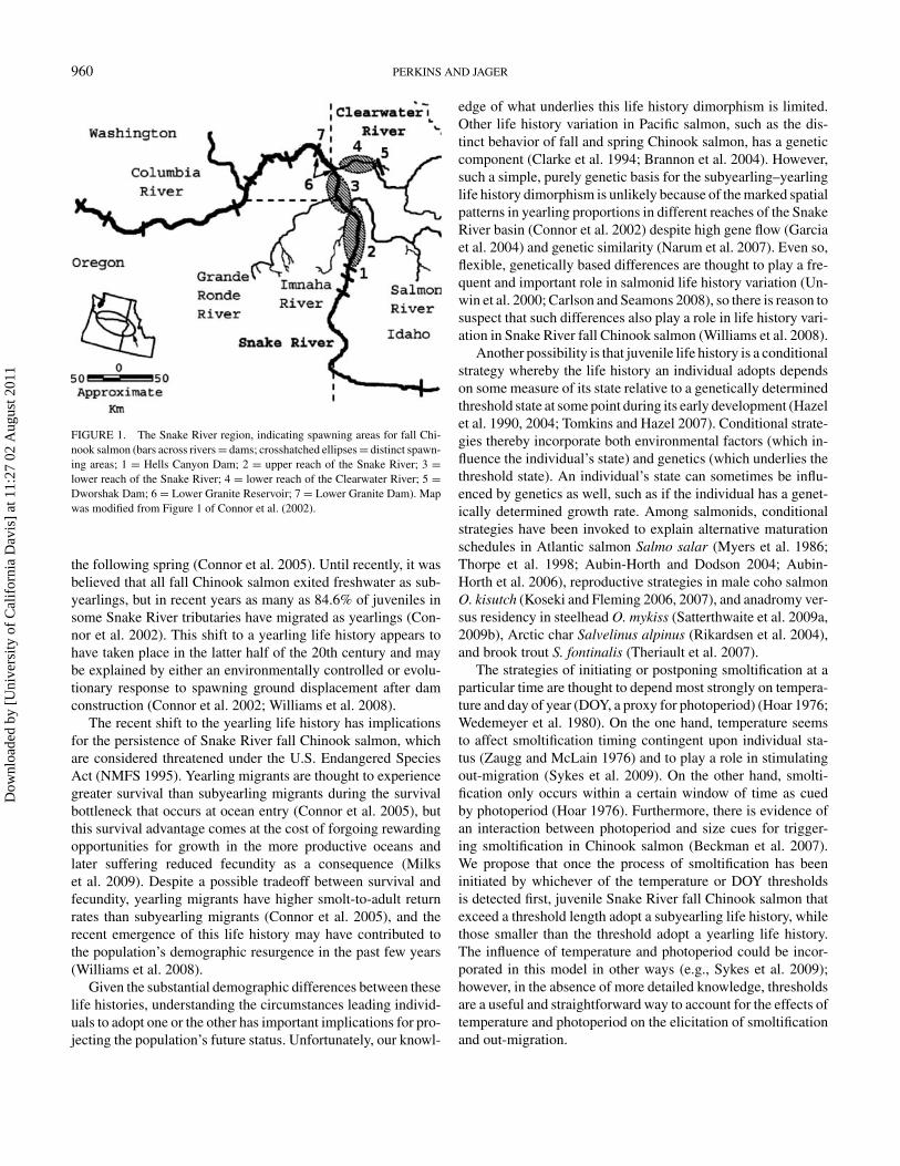
FIGURE 1. The Snake River region, indicating spawning areas for fall Chi-nook salmon (bars across rivers = dams; crosshatched ellipses = distinct spawn-ing areas; 1 = Hells Canyon Dam; 2 = upper reach of the Snake River; 3 =lower reach of the Snake River; 4 = lower reach of the Clearwater River; 5 =Dworshak Dam; 6 = Lower Granite Reservoir; 7 = Lower Granite Dam). Mapwas modified from Figure 1 of Connor et al. (2002).

the following spring (Connor et al. 2005). Until recently, it wasbelieved that all fall Chinook salmon exited freshwater as sub-yearlings, but in recent years as many as 84.6% of juveniles insome Snake River tributaries have migrated as yearlings (Con-nor et al. 2002). This shift to a yearling life history appears tohave taken place in the latter half of the 20th century and maybe explained by either an environmentally controlled or evolu-tionary response to spawning ground displacement after damconstruction (Connor et al. 2002; Williams et al. 2008).

The recent shift to the yearling life history has implicationsfor the persistence of Snake River fall Chinook salmon, whichare considered threatened under the U.S. Endangered SpeciesAct (NMFS 1995). Yearling migrants are thought to experiencegreater survival than subyearling migrants during the survivalbottleneck that occurs at ocean entry (Connor et al. 2005), butthis survival advantage comes at the cost of forgoing rewardingopportunities for growth in the more productive oceans andlater suffering reduced fecundity as a consequence (Milkset al. 2009). Despite a possible tradeoff between survival andfecundity, yearling migrants have higher smolt-to-adult returnrates than subyearling migrants (Connor et al. 2005), and therecent emergence of this life history may have contributed tothe population’s demographic resurgence in the past few years(Williams et al. 2008).

Given the substantial demographic differences between theselife histories, understanding the circumstances leading individ-uals to adopt one or the other has important implications for pro-jecting the population’s future status. Unfortunately, our knowl-

edge of what underlies this life history dimorphism is limited.Other life history variation in Pacific salmon, such as the dis-tinct behavior of fall and spring Chinook salmon, has a geneticcomponent (Clarke et al. 1994; Brannon et al. 2004). However,such a simple, purely genetic basis for the subyearling–yearlinglife history dimorphism is unlikely because of the marked spatialpatterns in yearling proportions in different reaches of the SnakeRiver basin (Connor et al. 2002) despite high gene flow (Garciaet al. 2004) and genetic similarity (Narum et al. 2007). Even so,flexible, genetically based differences are thought to play a fre-quent and important role in salmonid life history variation (Un-win et al. 2000; Carlson and Seamons 2008), so there is reason tosuspect that such differences also play a role in life history vari-ation in Snake River fall Chinook salmon (Williams et al. 2008).

Another possibility is that juvenile life history is a conditionalstrategy whereby the life history an individual adopts dependson some measure of its state relative to a genetically determinedthreshold state at some point during its early development (Hazelet al. 1990, 2004; Tomkins and Hazel 2007). Conditional strate-gies thereby incorporate both environmental factors (which in-fluence the individual’s state) and genetics (which underlies thethreshold state). An individual’s state can sometimes be influ-enced by genetics as well, such as if the individual has a genet-ically determined growth rate. Among salmonids, conditionalstrategies have been invoked to explain alternative maturationschedules in Atlantic salmon Salmo salar (Myers et al. 1986;Thorpe et al. 1998; Aubin-Horth and Dodson 2004; Aubin-Horth et al. 2006), reproductive strategies in male coho salmonO. kisutch (Koseki and Fleming 2006, 2007), and anadromy ver-sus residency in steelhead O. mykiss (Satterthwaite et al. 2009a,2009b), Arctic char Salvelinus alpinus (Rikardsen et al. 2004),and brook trout S. fontinalis (Theriault et al. 2007).

The strategies of initiating or postponing smoltification at aparticular time are thought to depend most strongly on tempera-ture and day of year (DOY, a proxy for photoperiod) (Hoar 1976;Wedemeyer et al. 1980). On the one hand, temperature seemsto affect smoltification timing contingent upon individual sta-tus (Zaugg and McLain 1976) and to play a role in stimulatingout-migration (Sykes et al. 2009). On the other hand, smolti-fication only occurs within a certain window of time as cuedby photoperiod (Hoar 1976). Furthermore, there is evidence ofan interaction between photoperiod and size cues for trigger-ing smoltification in Chinook salmon (Beckman et al. 2007).We propose that once the process of smoltification has beeninitiated by whichever of the temperature or DOY thresholdsis detected first, juvenile Snake River fall Chinook salmon thatexceed a threshold length adopt a subyearling life history, whilethose smaller than the threshold adopt a yearling life history.The influence of temperature and photoperiod could be incor-porated in this model in other ways (e.g., Sykes et al. 2009);however, in the absence of more detailed knowledge, thresholdsare a useful and straightforward way to account for the effects oftemperature and photoperiod on the elicitation of smoltificationand out-migration.

Dow

nloa

ded

by [

Uni

vers

ity o

f C

alif

orni

a D

avis

] at

11:

27 0

2 A

ugus

t 201

1

DELAYED GROWTH IN CHINOOK SALMON 961

In this paper, we postulate a model in which juvenile lifehistory of Snake River fall Chinook salmon is determined as aconditional strategy. We optimized this model to identify whichvalues of genetically determined length, temperature, and DOYthresholds lead to yearling migrant proportions that are mostconsistent with the empirical estimates reported by Connor et al.(2002). We also evaluated model performance and its sensitiv-ity to these three parameters as well as emergence timing andlength at emergence. Finally, we asked how different assump-tions about overwinter survival, which in turn lead to differentinterpretations of the data, influence the choice of thresholdvalues that are most consistent with empirical patterns.

METHODS

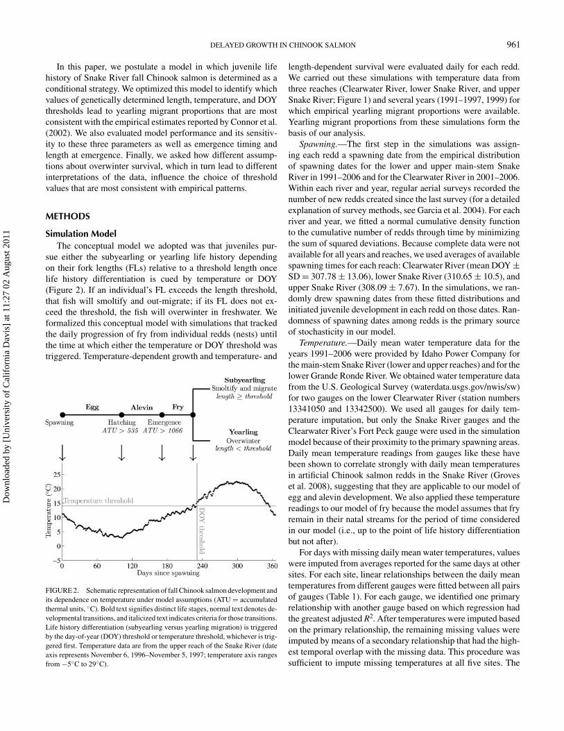
Simulation ModelThe conceptual model we adopted was that juveniles pur-

sue either the subyearling or yearling life history dependingon their fork lengths (FLs) relative to a threshold length oncelife history differentiation is cued by temperature or DOY(Figure 2). If an individual’s FL exceeds the length threshold,that fish will smoltify and out-migrate; if its FL does not ex-ceed the threshold, the fish will overwinter in freshwater. Weformalized this conceptual model with simulations that trackedthe daily progression of fry from individual redds (nests) untilthe time at which either the temperature or DOY threshold wastriggered. Temperature-dependent growth and temperature- and

FIGURE 2. Schematic representation of fall Chinook salmon development andits dependence on temperature under model assumptions (ATU = accumulatedthermal units, ◦C). Bold text signifies distinct life stages, normal text denotes de-velopmental transitions, and italicized text indicates criteria for those transitions.Life history differentiation (subyearling versus yearling migration) is triggeredby the day-of-year (DOY) threshold or temperature threshold, whichever is trig-gered first. Temperature data are from the upper reach of the Snake River (dateaxis represents November 6, 1996–November 5, 1997; temperature axis rangesfrom −5◦C to 29◦C).

length-dependent survival were evaluated daily for each redd.We carried out these simulations with temperature data fromthree reaches (Clearwater River, lower Snake River, and upperSnake River; Figure 1) and several years (1991–1997, 1999) forwhich empirical yearling migrant proportions were available.Yearling migrant proportions from these simulations form thebasis of our analysis.

Spawning.—The first step in the simulations was assign-ing each redd a spawning date from the empirical distributionof spawning dates for the lower and upper main-stem SnakeRiver in 1991–2006 and for the Clearwater River in 2001–2006.Within each river and year, regular aerial surveys recorded thenumber of new redds created since the last survey (for a detailedexplanation of survey methods, see Garcia et al. 2004). For eachriver and year, we fitted a normal cumulative density functionto the cumulative number of redds through time by minimizingthe sum of squared deviations. Because complete data were notavailable for all years and reaches, we used averages of availablespawning times for each reach: Clearwater River (mean DOY ±SD = 307.78 ± 13.06), lower Snake River (310.65 ± 10.5), andupper Snake River (308.09 ± 7.67). In the simulations, we ran-domly drew spawning dates from these fitted distributions andinitiated juvenile development in each redd on those dates. Ran-domness of spawning dates among redds is the primary sourceof stochasticity in our model.

Temperature.—Daily mean water temperature data for theyears 1991–2006 were provided by Idaho Power Company forthe main-stem Snake River (lower and upper reaches) and for thelower Grande Ronde River. We obtained water temperature datafrom the U.S. Geological Survey (waterdata.usgs.gov/nwis/sw)for two gauges on the lower Clearwater River (station numbers13341050 and 13342500). We used all gauges for daily tem-perature imputation, but only the Snake River gauges and theClearwater River’s Fort Peck gauge were used in the simulationmodel because of their proximity to the primary spawning areas.Daily mean temperature readings from gauges like these havebeen shown to correlate strongly with daily mean temperaturesin artificial Chinook salmon redds in the Snake River (Groveset al. 2008), suggesting that they are applicable to our model ofegg and alevin development. We also applied these temperaturereadings to our model of fry because the model assumes that fryremain in their natal streams for the period of time consideredin our model (i.e., up to the point of life history differentiationbut not after).

For days with missing daily mean water temperatures, valueswere imputed from averages reported for the same days at othersites. For each site, linear relationships between the daily meantemperatures from different gauges were fitted between all pairsof gauges (Table 1). For each gauge, we identified one primaryrelationship with another gauge based on which regression hadthe greatest adjusted R2. After temperatures were imputed basedon the primary relationship, the remaining missing values wereimputed by means of a secondary relationship that had the high-est temporal overlap with the missing data. This procedure wassufficient to impute missing temperatures at all five sites. The

Dow

nloa

ded

by [

Uni

vers

ity o

f C

alif

orni

a D

avis

] at

11:

27 0

2 A

ugus

t 201

1

962 PERKINS AND JAGER

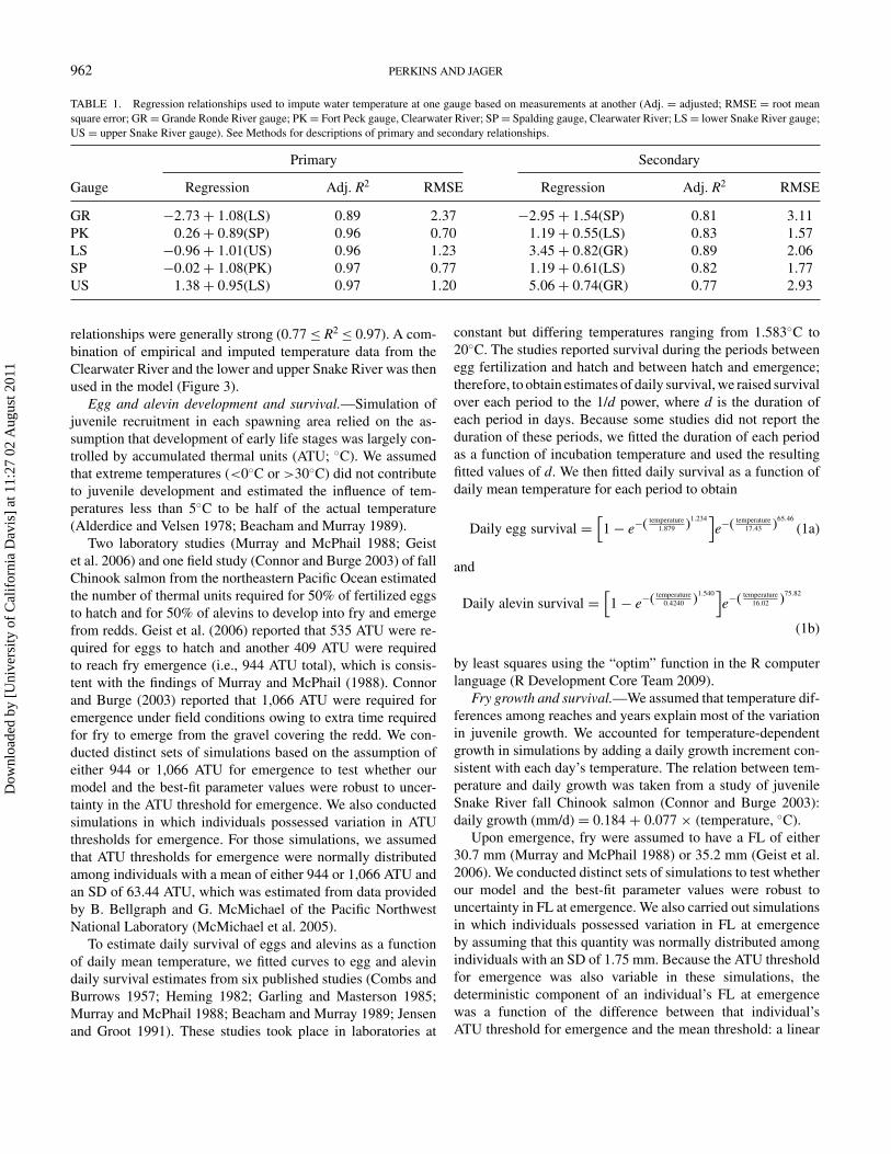
TABLE 1. Regression relationships used to impute water temperature at one gauge based on measurements at another (Adj. = adjusted; RMSE = root meansquare error; GR = Grande Ronde River gauge; PK = Fort Peck gauge, Clearwater River; SP = Spalding gauge, Clearwater River; LS = lower Snake River gauge;US = upper Snake River gauge). See Methods for descriptions of primary and secondary relationships.

Primary Secondary

Gauge Regression Adj. R2 RMSE Regression Adj. R2 RMSE

GR −2.73 + 1.08(LS) 0.89 2.37 −2.95 + 1.54(SP) 0.81 3.11PK 0.26 + 0.89(SP) 0.96 0.70 1.19 + 0.55(LS) 0.83 1.57LS −0.96 + 1.01(US) 0.96 1.23 3.45 + 0.82(GR) 0.89 2.06SP −0.02 + 1.08(PK) 0.97 0.77 1.19 + 0.61(LS) 0.82 1.77US 1.38 + 0.95(LS) 0.97 1.20 5.06 + 0.74(GR) 0.77 2.93

relationships were generally strong (0.77 ≤ R2 ≤ 0.97). A com-bination of empirical and imputed temperature data from theClearwater River and the lower and upper Snake River was thenused in the model (Figure 3).

Egg and alevin development and survival.—Simulation ofjuvenile recruitment in each spawning area relied on the as-sumption that development of early life stages was largely con-trolled by accumulated thermal units (ATU; ◦C). We assumedthat extreme temperatures (<0◦C or >30◦C) did not contributeto juvenile development and estimated the influence of tem-peratures less than 5◦C to be half of the actual temperature(Alderdice and Velsen 1978; Beacham and Murray 1989).

Two laboratory studies (Murray and McPhail 1988; Geistet al. 2006) and one field study (Connor and Burge 2003) of fallChinook salmon from the northeastern Pacific Ocean estimatedthe number of thermal units required for 50% of fertilized eggsto hatch and for 50% of alevins to develop into fry and emergefrom redds. Geist et al. (2006) reported that 535 ATU were re-quired for eggs to hatch and another 409 ATU were requiredto reach fry emergence (i.e., 944 ATU total), which is consis-tent with the findings of Murray and McPhail (1988). Connorand Burge (2003) reported that 1,066 ATU were required foremergence under field conditions owing to extra time requiredfor fry to emerge from the gravel covering the redd. We con-ducted distinct sets of simulations based on the assumption ofeither 944 or 1,066 ATU for emergence to test whether ourmodel and the best-fit parameter values were robust to uncer-tainty in the ATU threshold for emergence. We also conductedsimulations in which individuals possessed variation in ATUthresholds for emergence. For those simulations, we assumedthat ATU thresholds for emergence were normally distributedamong individuals with a mean of either 944 or 1,066 ATU andan SD of 63.44 ATU, which was estimated from data providedby B. Bellgraph and G. McMichael of the Pacific NorthwestNational Laboratory (McMichael et al. 2005).

To estimate daily survival of eggs and alevins as a functionof daily mean temperature, we fitted curves to egg and alevindaily survival estimates from six published studies (Combs andBurrows 1957; Heming 1982; Garling and Masterson 1985;Murray and McPhail 1988; Beacham and Murray 1989; Jensenand Groot 1991). These studies took place in laboratories at

constant but differing temperatures ranging from 1.583◦C to20◦C. The studies reported survival during the periods betweenegg fertilization and hatch and between hatch and emergence;therefore, to obtain estimates of daily survival, we raised survivalover each period to the 1/d power, where d is the duration ofeach period in days. Because some studies did not report theduration of these periods, we fitted the duration of each periodas a function of incubation temperature and used the resultingfitted values of d. We then fitted daily survival as a function ofdaily mean temperature for each period to obtain

Daily egg survival =[1 − e−( temperature

1.879 )1.234]e−( temperature

17.43 )65.46

(1a)

and

Daily alevin survival =[1 − e−( temperature

0.4240 )1.540]e−( temperature

16.02 )75.82

(1b)

by least squares using the “optim” function in the R computerlanguage (R Development Core Team 2009).

Fry growth and survival.—We assumed that temperature dif-ferences among reaches and years explain most of the variationin juvenile growth. We accounted for temperature-dependentgrowth in simulations by adding a daily growth increment con-sistent with each day’s temperature. The relation between tem-perature and daily growth was taken from a study of juvenileSnake River fall Chinook salmon (Connor and Burge 2003):daily growth (mm/d) = 0.184 + 0.077 × (temperature, ◦C).

Upon emergence, fry were assumed to have a FL of either30.7 mm (Murray and McPhail 1988) or 35.2 mm (Geist et al.2006). We conducted distinct sets of simulations to test whetherour model and the best-fit parameter values were robust touncertainty in FL at emergence. We also carried out simulationsin which individuals possessed variation in FL at emergenceby assuming that this quantity was normally distributed amongindividuals with an SD of 1.75 mm. Because the ATU thresholdfor emergence was also variable in these simulations, thedeterministic component of an individual’s FL at emergencewas a function of the difference between that individual’sATU threshold for emergence and the mean threshold: a linear

Dow

nloa

ded

by [

Uni

vers

ity o

f C

alif

orni

a D

avis

] at

11:

27 0

2 A

ugus

t 201

1

DELAYED GROWTH IN CHINOOK SALMON 963

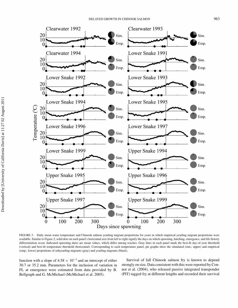
FIGURE 3. Daily mean water temperature and Chinook salmon yearling migrant proportions for years in which empirical yearling migrant proportions wereavailable. Similar to Figure 2, solid dots on each panel’s horizontal axis from left to right signify the days on which spawning, hatching, emergence, and life historydifferentiation occur. Indicated spawning dates are mean values, which differ among reaches. Gray lines in each panel mark the best-fit day-of-year threshold(vertical) and best-fit temperature threshold (horizontal). Corresponding to each temperature panel, pie graphs show the simulated (sim.; upper) and empirical(emp.; lower) proportions of subyearling migrants (gray) and yearling migrants (black).

function with a slope of 4.58 × 10−3 and an intercept of either30.7 or 35.2 mm. Parameters for the inclusion of variation inFL at emergence were estimated from data provided by B.Bellgraph and G. McMichael (McMichael et al. 2005).

Survival of fall Chinook salmon fry is known to dependstrongly on size. Data consistent with this were reported by Con-nor et al. (2004), who released passive integrated transponder(PIT) tagged fry at different lengths and recorded their survival

Dow

nloa

ded

by [

Uni

vers

ity o

f C

alif

orni

a D

avis

] at

11:

27 0

2 A

ugus

t 201

1

964 PERKINS AND JAGER

upon passage at Lower Granite Dam. To translate survival be-tween release and passage at the dam (encompassing a periodof several weeks) to an estimate of daily survival, we fitted datafrom Connor et al. (2004) to obtain the relationship

Daily fry survival = 0.99 − (0.99 − 0.96)e−( FL91.445 )100

, (2)

where FL is in millimeters. Fitted parameter values in equation(2) differed based on assumptions about the ATU threshold forfry emergence and FL at emergence, but fitted values were inagreement with the precision in equation (2) and R2 was 0.98or greater in all cases. Details of the procedure used to obtainthis formula are presented in the Appendix. Daily survival fromequation (2) was applied to simulated fry every day betweenemergence from the gravel and the date of life history differen-tiation. Connor et al. (2000) estimated a survival probability thatwas dependent on FL, the date of life history differentiation, andmean temperature on that day; this probability was then appliedto newly differentiated fry to account for mortality between de-parture from their natal stream and migration past lower GraniteDam. The numbers of surviving subyearlings and yearlings werethen used to calculate simulated yearling migrant proportions.

Threshold Parameter EstimationTo determine which combination of threshold parameter val-

ues produced simulated yearling migrant proportions that weremost consistent with observations, we searched for a best-fitparameter combination that minimized the sum of squared dif-ferences (i.e., sum of squares [SSQ]) between simulated (sim)and empirically estimated (emp) yearling migrant proportionssummed over all years t and all reaches x as follows:

SSQ(D,L, T ) =∑∀t,x

[sim(t, x; D,L, T ) − emp(t, x)]2, (3)

where D represents the DOY threshold, L is the FL thresh-old, and T is the temperature threshold. Quantitatively, an SSQvalue of 0 implies a perfect correspondence between simulatedand empirically estimated yearling migrant proportions; SSQequals 1.31 when all simulated juveniles migrate as subyear-lings, equals 12.61 when all simulated juveniles migrate as year-lings, and is between 0 and 12.61 when simulated juveniles area mixture of life histories. To search for the best-fit parametercombination, we conducted a global optimization by completeenumeration. Specifically, we considered every other integer ofD in the range of 121–273, L-values of 31–150 mm in incrementsof 2 mm, and T-values of 12–22◦C in increments of 0.5◦C.

Overwinter SurvivalConnor et al. (2002) defined the yearling migrant proportion

(p) as

p = y

s + y, (4)

where s and y are the number of subyearlings and yearlings fromthe same cohort that were recorded as passing Lower GraniteDam. More precisely, s is the number of PIT-tagged fish releasedin year t that pass Lower Granite Dam in year t, and y is thenumber of PIT-tagged fish released in year t that pass LowerGranite Dam in year t + 1.

To estimate the proportion of juveniles that initially adopt ayearling life history (p′), we first noted that the initial numberof subyearlings (s′) is equal to s and that the initial number ofyearlings (y′) is equal to y/u, where u is the survival of year-ling migrants between the time they commit to that life historystrategy and the time of passage at Lower Granite Dam (i.e.,overwinter survival). It follows that p′ is calculated as

p′ = y ′

s ′ + y ′ , (5)

which can be written in terms of the empirically estimated pro-portion p and unknown u as

p′ =(

1 − u + u

p

)−1

. (6)

The term u accounts for mortality risks posed over a periodof several months in potentially harsh environments. Becauseu-values less than 1 could mean that p′ and p are quite different,we explored how u affects p′ for empirically estimated values ofp. Moreover, because a primary goal of our investigation was toestimate values for the thresholds underlying the adoption of onelife history or the other, we determined the thresholds’ sensitiv-ities to u by exploring how relative differences in SSQ amongdifferent threshold parameter values changed with a range ofu-values (1.00, 0.75, 0.50, and 0.25).

RESULTSWe identified the following thresholds as those providing

the best match to empirically estimated life history proportionsunder the assumption of zero overwinter mortality: the best-fitDOY threshold (D*) was 167–211, the best-fit length thresh-old (L*) was 35–48 mm, and the best-fit temperature threshold(T*) was 14.0◦C (Table 2). Underlying this range of best-fitvalues is uncertainty in the ATU threshold for emergence, FLat emergence, and the existence of individual variation in thosequantities. Despite uncertainty in these parameters, some gen-eralities about the best-fit values are that (1) D* is so great asto make it inapplicable for most reaches and years; (2) when-ever D* triggers life history differentiation, it does so no morethan 10 d before a temperature threshold is triggered; (3) L*is only 5–13 mm greater than FL at emergence; and (4) T* isalways 14.0◦C. In all subsequent analyses, we focus on the setof best-fit thresholds (D* = 177, L* = 40 mm, and T* = 14◦C;fourth data column of Table 2) that corresponded to the most

Dow

nloa

ded

by [

Uni

vers

ity o

f C

alif

orni

a D

avis

] at

11:

27 0

2 A

ugus

t 201

1

DELAYED GROWTH IN CHINOOK SALMON 965

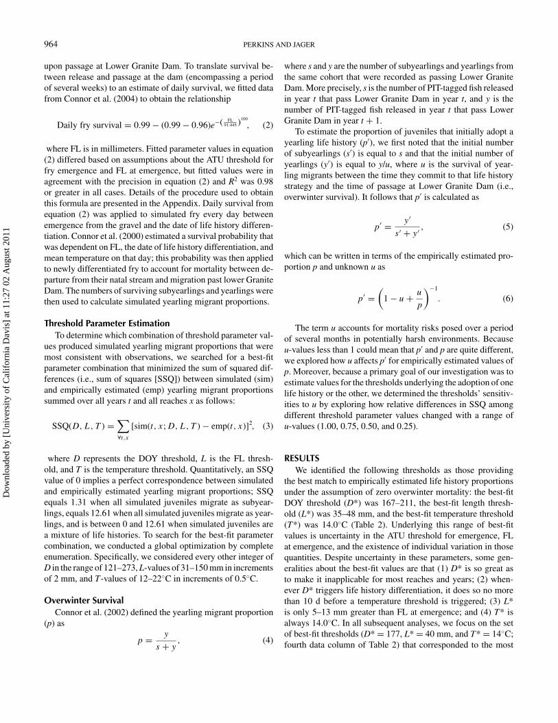
TABLE 2. Best-fit thresholds (D* = day-of-year [DOY] threshold; L* = fork length [FL] threshold, mm; T* = temperature threshold, ◦C) under differentassumptions about the accumulated thermal unit (ATU) threshold for Chinook salmon fry emergence, the FL at emergence, and the existence of individual variationin those parameters. Due to higher computational demands, a D* value of 253 was used in simulations with variation in emergence ATU and FL to constrain thebest-fit parameter search to a single DOY threshold that is never attained.

Variation in emergence ATU and FL?

No Yes

944 ATU 1,066 ATU 944 ATU 1,066 ATU

Threshold 30.7 mm 35.2 mm 30.7 mm 35.2 mm 30.7 mm 35.2 mm 30.7 mm 35.2 mm

D* 169 167 211 177L* 41 46 35 40 45 48 35 40T* 14 14 14 14 14 14 14 14

realistic scenario about the ATU threshold for emergence andFL at emergence under field conditions.

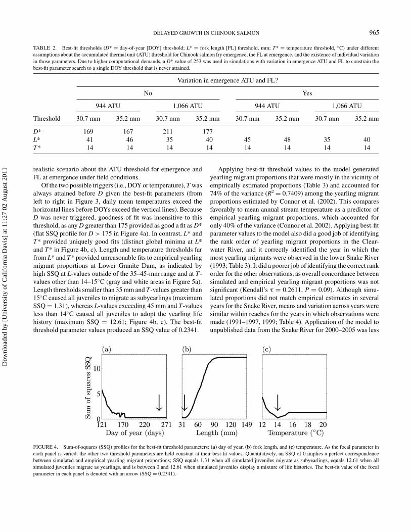
Of the two possible triggers (i.e., DOY or temperature), T wasalways attained before D given the best-fit parameters (fromleft to right in Figure 3, daily mean temperatures exceed thehorizontal lines before DOYs exceed the vertical lines). BecauseD was never triggered, goodness of fit was insensitive to thisthreshold, as any D greater than 175 provided as good a fit as D*(flat SSQ profile for D > 175 in Figure 4a). In contrast, L* andT* provided uniquely good fits (distinct global minima at L*and T* in Figure 4b, c). Length and temperature thresholds farfrom L* and T* provided unreasonable fits to empirical yearlingmigrant proportions at Lower Granite Dam, as indicated byhigh SSQ at L-values outside of the 35–45-mm range and at T-values other than 14–15◦C (gray and white areas in Figure 5a).Length thresholds smaller than 35 mm and T-values greater than15◦C caused all juveniles to migrate as subyearlings (maximumSSQ = 1.31), whereas L-values exceeding 45 mm and T-valuesless than 14◦C caused all juveniles to adopt the yearling lifehistory (maximum SSQ = 12.61; Figure 4b, c). The best-fitthreshold parameter values produced an SSQ value of 0.2341.

Applying best-fit threshold values to the model generatedyearling migrant proportions that were mostly in the vicinity ofempirically estimated proportions (Table 3) and accounted for74% of the variance (R2 = 0.7409) among the yearling migrantproportions estimated by Connor et al. (2002). This comparesfavorably to mean annual stream temperature as a predictor ofempirical yearling migrant proportions, which accounted foronly 40% of the variance (Connor et al. 2002). Applying best-fitparameter values to the model also did a good job of identifyingthe rank order of yearling migrant proportions in the Clear-water River, and it correctly identified the year in which themost yearling migrants were observed in the lower Snake River(1993; Table 3). It did a poorer job of identifying the correct rankorder for the other observations, as overall concordance betweensimulated and empirical yearling migrant proportions was notsignificant (Kendall’s τ = 0.2611, P = 0.09). Although simu-lated proportions did not match empirical estimates in severalyears for the Snake River, means and variation across years weresimilar within reaches for the years in which observations weremade (1991–1997, 1999; Table 4). Application of the model tounpublished data from the Snake River for 2000–2005 was less

FIGURE 4. Sum-of-squares (SSQ) profiles for the best-fit threshold parameters: (a) day of year, (b) fork length, and (c) temperature. As the focal parameter ineach panel is varied, the other two threshold parameters are held constant at their best-fit values. Quantitatively, an SSQ of 0 implies a perfect correspondencebetween simulated and empirical yearling migrant proportions; SSQ equals 1.31 when all simulated juveniles migrate as subyearlings, equals 12.61 when allsimulated juveniles migrate as yearlings, and is between 0 and 12.61 when simulated juveniles display a mixture of life histories. The best-fit value of the focalparameter in each panel is denoted with an arrow (SSQ = 0.2341).

Dow

nloa

ded

by [

Uni

vers

ity o

f C

alif

orni

a D

avis

] at

11:

27 0

2 A

ugus

t 201

1

966 PERKINS AND JAGER

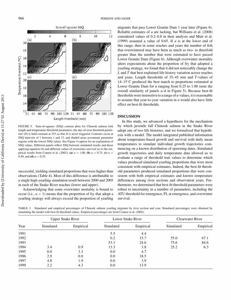
FIGURE 5. Sum-of-squares (SSQ) contour plots for Chinook salmon forklength and temperature threshold parameters; the day-of-year threshold param-eter (D) is held constant at 253 so that D is never triggered. Contours occur atSSQ intervals of 1 between 1 and 12, and shaded areas accentuate parameterregions with the lowest SSQ values. See Figure 4 caption for an explanation ofSSQ values. Different panels reflect SSQ between simulated results and thoseapplying equation (6) and different values of overwinter survival (u) to the em-pirical results from Connor et al. (2002): (a) u = 1.00, (b) u = 0.75, (c) u =0.50, and (d) u = 0.25.

successful, yielding simulated proportions that were higher thanobservations (Table 4). Most of this difference is attributable toa single high-yearling simulation result between 2000 and 2005in each of the Snake River reaches (lower and upper).

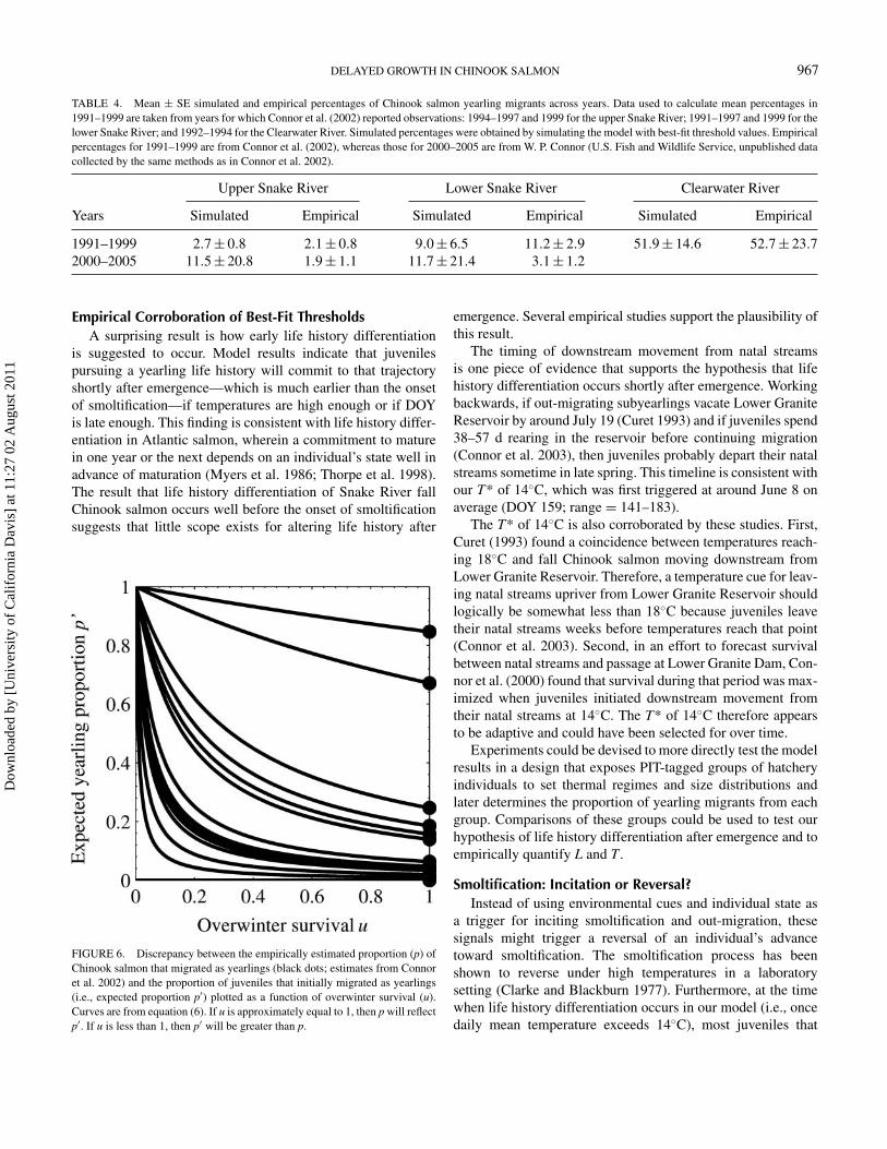
Acknowledging that some overwinter mortality is bound tooccur (i.e., u < 1) means that the proportion of fry that adopt ayearling strategy will always exceed the proportion of yearling

migrants that pass Lower Granite Dam 1 year later (Figure 6).Reliable estimates of u are lacking, but Williams et al. (2008)considered values of 0.2–0.8 in their analysis and Muir et al.(1999) assumed a value of 0.65. If u is at the lower end ofthis range, then in some reaches and years the number of fishthat overwintered may have been as much as two- to threefoldgreater than the number that were estimated to have passedLower Granite Dam (Figure 6). Although overwinter mortalityalters expectations about the proportion of fry that adopted ayearling strategy, we found that it did not noticeably change theL and T that best explained life history variation across reachesand years. Length thresholds of 35–45 mm and T-values of14–15◦C produced the best match to proportions estimated atLower Granite Dam for u ranging from 0.25 to 1.00 (note theoverall similarity of panels a–d in Figure 5). Because best-fitthresholds were insensitive to a range of u-values, it is reasonableto assume that year-to-year variation in u would also have littleeffect on best-fit thresholds.

DISCUSSIONIn this study, we advanced a hypothesis for the mechanism

by which juvenile fall Chinook salmon in the Snake Riveradopt one of two life histories, and we formalized that hypoth-esis with a model. The model integrated published informationabout temperature-based growth and survival with daily meantemperatures to simulate individual growth trajectories com-mencing on a known distribution of spawning dates. Simulatedgrowth trajectories and daily temperature data allowed us toevaluate a range of threshold trait values to determine whichvalues produced simulated yearling proportions that were mostconsistent with empirical estimates. Indeed, the best-fit thresh-old parameters produced simulated proportions that were con-sistent with both empirical estimates and known temperaturedifferences among river sections and observation years. Fur-thermore, we determined that best-fit threshold parameters wererobust to uncertainty in a number of parameters, including theATU threshold for emergence, FL at emergence, and overwintersurvival.

TABLE 3. Simulated and empirical percentages of Chinook salmon yearling migrants by river section and year. Simulated percentages were obtained bysimulating the model with best-fit threshold values. Empirical percentages are from Connor et al. (2002).

Upper Snake River Lower Snake River Clearwater River

Year Simulated Empirical Simulated Empirical Simulated Empirical

1991 5.5 4.41992 0.2 15.7 55.0 67.11993 53.1 24.6 75.6 84.61994 3.4 0.9 13.3 3.8 25.2 6.31995 0.0 3.3 0.0 4.71996 2.9 0.0 0.0 18.51997 4.8 1.9 0.0 3.91999 2.2 4.3 0.0 13.9

Dow

nloa

ded

by [

Uni

vers

ity o

f C

alif

orni

a D

avis

] at

11:

27 0

2 A

ugus

t 201

1

DELAYED GROWTH IN CHINOOK SALMON 967

TABLE 4. Mean ± SE simulated and empirical percentages of Chinook salmon yearling migrants across years. Data used to calculate mean percentages in1991–1999 are taken from years for which Connor et al. (2002) reported observations: 1994–1997 and 1999 for the upper Snake River; 1991–1997 and 1999 for thelower Snake River; and 1992–1994 for the Clearwater River. Simulated percentages were obtained by simulating the model with best-fit threshold values. Empiricalpercentages for 1991–1999 are from Connor et al. (2002), whereas those for 2000–2005 are from W. P. Connor (U.S. Fish and Wildlife Service, unpublished datacollected by the same methods as in Connor et al. 2002).

Upper Snake River Lower Snake River Clearwater River

Years Simulated Empirical Simulated Empirical Simulated Empirical

1991–1999 2.7 ± 0.8 2.1 ± 0.8 9.0 ± 6.5 11.2 ± 2.9 51.9 ± 14.6 52.7 ± 23.72000–2005 11.5 ± 20.8 1.9 ± 1.1 11.7 ± 21.4 3.1 ± 1.2

Empirical Corroboration of Best-Fit ThresholdsA surprising result is how early life history differentiation

is suggested to occur. Model results indicate that juvenilespursuing a yearling life history will commit to that trajectoryshortly after emergence—which is much earlier than the onsetof smoltification—if temperatures are high enough or if DOYis late enough. This finding is consistent with life history differ-entiation in Atlantic salmon, wherein a commitment to maturein one year or the next depends on an individual’s state well inadvance of maturation (Myers et al. 1986; Thorpe et al. 1998).The result that life history differentiation of Snake River fallChinook salmon occurs well before the onset of smoltificationsuggests that little scope exists for altering life history after

FIGURE 6. Discrepancy between the empirically estimated proportion (p) ofChinook salmon that migrated as yearlings (black dots; estimates from Connoret al. 2002) and the proportion of juveniles that initially migrated as yearlings(i.e., expected proportion p′) plotted as a function of overwinter survival (u).Curves are from equation (6). If u is approximately equal to 1, then p will reflectp′. If u is less than 1, then p′ will be greater than p.

emergence. Several empirical studies support the plausibility ofthis result.

The timing of downstream movement from natal streamsis one piece of evidence that supports the hypothesis that lifehistory differentiation occurs shortly after emergence. Workingbackwards, if out-migrating subyearlings vacate Lower GraniteReservoir by around July 19 (Curet 1993) and if juveniles spend38–57 d rearing in the reservoir before continuing migration(Connor et al. 2003), then juveniles probably depart their natalstreams sometime in late spring. This timeline is consistent withour T* of 14◦C, which was first triggered at around June 8 onaverage (DOY 159; range = 141–183).

The T* of 14◦C is also corroborated by these studies. First,Curet (1993) found a coincidence between temperatures reach-ing 18◦C and fall Chinook salmon moving downstream fromLower Granite Reservoir. Therefore, a temperature cue for leav-ing natal streams upriver from Lower Granite Reservoir shouldlogically be somewhat less than 18◦C because juveniles leavetheir natal streams weeks before temperatures reach that point(Connor et al. 2003). Second, in an effort to forecast survivalbetween natal streams and passage at Lower Granite Dam, Con-nor et al. (2000) found that survival during that period was max-imized when juveniles initiated downstream movement fromtheir natal streams at 14◦C. The T* of 14◦C therefore appearsto be adaptive and could have been selected for over time.

Experiments could be devised to more directly test the modelresults in a design that exposes PIT-tagged groups of hatcheryindividuals to set thermal regimes and size distributions andlater determines the proportion of yearling migrants from eachgroup. Comparisons of these groups could be used to test ourhypothesis of life history differentiation after emergence and toempirically quantify L and T .

Smoltification: Incitation or Reversal?Instead of using environmental cues and individual state as

a trigger for inciting smoltification and out-migration, thesesignals might trigger a reversal of an individual’s advancetoward smoltification. The smoltification process has beenshown to reverse under high temperatures in a laboratorysetting (Clarke and Blackburn 1977). Furthermore, at the timewhen life history differentiation occurs in our model (i.e., oncedaily mean temperature exceeds 14◦C), most juveniles that

Dow

nloa

ded

by [

Uni

vers

ity o

f C

alif

orni

a D

avis

] at

11:

27 0

2 A

ugus

t 201

1

968 PERKINS AND JAGER

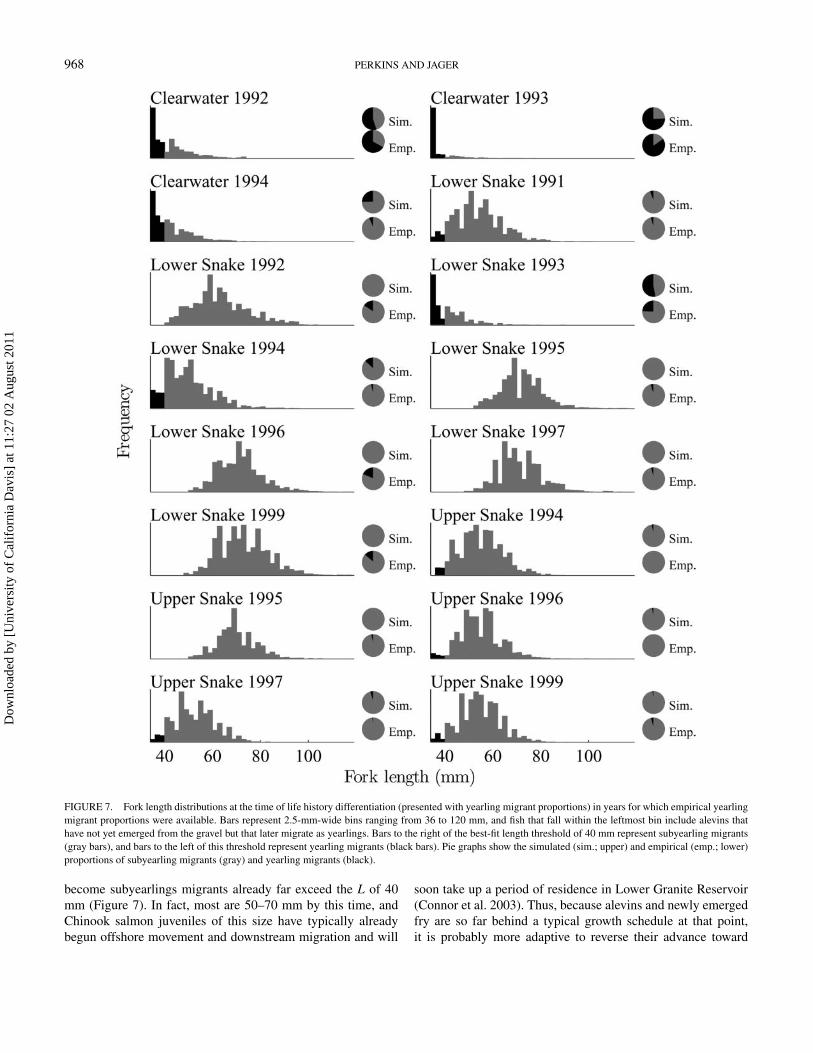
FIGURE 7. Fork length distributions at the time of life history differentiation (presented with yearling migrant proportions) in years for which empirical yearlingmigrant proportions were available. Bars represent 2.5-mm-wide bins ranging from 36 to 120 mm, and fish that fall within the leftmost bin include alevins thathave not yet emerged from the gravel but that later migrate as yearlings. Bars to the right of the best-fit length threshold of 40 mm represent subyearling migrants(gray bars), and bars to the left of this threshold represent yearling migrants (black bars). Pie graphs show the simulated (sim.; upper) and empirical (emp.; lower)proportions of subyearling migrants (gray) and yearling migrants (black).

become subyearlings migrants already far exceed the L of 40mm (Figure 7). In fact, most are 50–70 mm by this time, andChinook salmon juveniles of this size have typically alreadybegun offshore movement and downstream migration and will

soon take up a period of residence in Lower Granite Reservoir(Connor et al. 2003). Thus, because alevins and newly emergedfry are so far behind a typical growth schedule at that point,it is probably more adaptive to reverse their advance toward

Dow

nloa

ded

by [

Uni

vers

ity o

f C

alif

orni

a D

avis

] at

11:

27 0

2 A

ugus

t 201

1

DELAYED GROWTH IN CHINOOK SALMON 969

smoltification, overwinter in freshwater, and migrate as year-lings than to pursue the typical subyearling migration course.

The hypothesis that developing juveniles reverse course ifthey fall behind a typical growth schedule allows for the pos-sibility that there are multiple opportunities for such a reversalover a fish’s development. Additional opportunities for over-wintering beyond the 14◦C threshold could account for severalinstances where the model predicts fewer yearling migrants thanwere empirically estimated. Specifically, in the lower SnakeRiver during 1992, 1996, and 1999, the size distribution thatwas present when the T of 14◦C was first attained was quite farahead of where it should have been to produce the empiricallyestimated yearling migrant proportions (Figure 7). However, ifgrowth thereafter is slowed by cool temperatures or lack of food,some of those fish may fall behind the typical growth scheduleand may opt to overwinter once another temperature or DOYthreshold is reached, thus accounting for the individuals thatwere counted as yearling migrants. That these decisions couldbe made at any point during downstream migration is consis-tent with the hypothesis that some juveniles might decide tooverwinter later on at any number of reservoirs between LowerGranite Dam and the ocean (Connor et al. 2002; Buchanan et al.2009). Although it may be more realistic to say that individ-ual growth is assessed against multiple thresholds at multiplecheckpoints during development, our results support the hypoth-esis that life history differentiation occurs only once: soon afteremergence. Empirical yearling migrant proportions for reser-voirs downstream from Lower Granite Dam could help to deter-mine whether such a “wait-and-see” strategy occurs by similarmeans as the “decide-early” strategy we propose here, but datawith which to test that hypothesis are not currently available.

Demographic ImplicationsOne of the primary motivations for research on juvenile life

history of Snake River fall Chinook salmon is its relevance tothe recent resurgence and hopeful recovery of this population(Williams et al. 2008). Maximizing the utility of our model formanagers will therefore require integration of the model within apopulation viability analysis. Such an effort could shed light onthe effects of different degrees of life history variation on thispopulation’s extinction risk, telling us whether the increasedprevalence of yearling migrants will benefit the population andwhat the implications of management actions are that affect lifehistories via temperature change. Given that our model providesa reasonable description of yearling migrant proportions withina reach averaged over time (similarity between simulated andempirical mean ± SE in Table 4), it is suitable for applicationto population viability analysis, where accounting for long-termvariation supersedes year-to-year prediction.

An important consideration for the management of anyspecies over the next several decades is climate change. Someof the changes anticipated for the interior Pacific Northwestthat could affect spawning and rearing areas in the Snake Riverbasin include milder winters and overall higher surface air tem-

peratures, which are in turn likely to generate a rise in streamtemperatures (Crozier et al. 2008). Based on our results, climatechange might affect this population’s life history in either oftwo ways. On the one hand, milder winters would lead to earlieremergence, earlier exceedance of L, and thus fewer yearling mi-grants. On the other hand, yearling migrant percentages couldincrease if T is exceeded earlier in the spring. Complicatingmatters further, effects of climate change on other aspects oflife history could also alter juvenile life history. Perhaps mostimportantly, changes in spawning date, which tends to be ex-tremely labile and heritable (Carlson and Seamons 2008), couldincrease or decrease yearling migrant percentages or possiblyeven buffer life history changes promoted by milder winters andunseasonably high temperature extremes.

Another factor that may influence the future life historystrategies exhibited by this population is hydropower (Wapleset al. 2008b). Changes in temperature and flow regimes fromhydropower manipulation have exerted marked selection pres-sures on Chinook salmon in Oregon (Angilletta et al. 2008),make possible over-summer residence in Lower Granite Reser-voir due to summer flow augmentation (Connor et al. 2003;Smith et al. 2003), and could exert additional influence in thefuture if dams are ever removed or abandoned (Williams et al.2008). In fact, the population’s displacement from its historicalspawning grounds due to dam construction is believed to haveinstigated the shift towards more yearling migrants in the firstplace (Connor et al. 2002; Williams et al. 2008). Cooler tem-peratures and lower food availability may have also contributedto this abrupt life history shift (Connor et al. 2002; Williamset al. 2008). In future work, our model could be used to inves-tigate the role of temperature differences between historic andpresent-day reaches in accounting for more yearling migrantsin the latter. In its present condition, the model is capable of ad-dressing the extent to which phenotypic plasticity accounts forincreased prevalence of yearling migrants between historic andpresent-day reaches, but the model could be developed furtherto investigate the role of genetically based evolution in this lifehistory shift (e.g., by adding heritable variation in thresholds orgrowth rates).

ACKNOWLEDGMENTSThis research was conducted at the Oak Ridge National Lab-

oratory, which is managed by UT-Battelle, LLC, under Con-tract Number DE-AC05-00OR22725 with the U.S. Departmentof Energy (DOE). The publisher, by accepting the article forpublication, acknowledges that the U.S. Government retains anonexclusive, paid-up, irrevocable, worldwide license to pub-lish or reproduce the published form of this manuscript, or al-low others to do so, for U.S. Government purposes. H.I.J. wasfunded by Idaho Power Company under U.S. DOE ContractNumber NFE-06-00450. T.A.P. was funded by a ComputationalSciences Graduate Fellowship, which is managed by Krell Insti-tute under U.S. DOE Contract Number DE-FG02-97ER25308.

Dow

nloa

ded

by [

Uni

vers

ity o

f C

alif

orni

a D

avis

] at

11:

27 0

2 A

ugus

t 201

1

970 PERKINS AND JAGER

We appreciate comments on the manuscript from G. Cada (OakRidge National Laboratory), J. Chandler, P. Groves, R. Waples,and an anonymous reviewer. J. Chandler and P. Groves pro-vided spawning and temperature data on behalf of Idaho PowerCompany; B. Bellgraph and G. McMichael provided data onvariation in fry emergence timing and FL; and W. P. Connor(U.S. Fish and Wildlife Service) provided life history data for2000–2005. Thanks are extended to A. Lockhart for assistancewith temperature imputation.

REFERENCESAlderdice, D., and F. Velsen. 1978. Relation between temperature and incubation

time for eggs of Chinook salmon (Oncorhynchus tshawytscha). Journal of theFisheries Research Board of Canada 35:69–75.

Angilletta, M., E. Steel, K. Bartz, J. Kingsolver, M. Scheuerell, B. Beckman, andL. Crozier. 2008. Big dams and salmon evolution: changes in thermal regimesand their potential evolutionary consequences. Evolutionary Applications1:286–299.

Aubin-Horth, N., J. Bourque, G. Daigle, R. Hedger, and J. Dodson. 2006.Longitudinal gradients in threshold sizes for alternative male life historytactics in a population of Atlantic salmon Salmo salar. Canadian Journal ofFisheries and Aquatic Sciences 63:2067–2075.

Aubin-Horth, N., and J. Dodson. 2004. Influence of individual body size andvariable thresholds on the incidence of a sneaker male reproductive tactic inAtlantic salmon. Evolution 58:136–144.

Beacham, T., and C. Murray. 1989. Variation in developmental biology ofsockeye salmon (Oncorhynchus nerka) and Chinook salmon (O. tshawytscha)in British Columbia. Canadian Journal of Zoology 67:2081–2089.

Beckman, B., B. Gadberry, P. Parkins, K. Cooper, and K. Arkush. 2007. State-dependent life history plasticity in Sacramento River winter-run Chinooksalmon (Oncorhynchus tshawytscha): interactions among photoperiod andgrowth modulate smolting and early male maturation. Canadian Journal ofFisheries and Aquatic Sciences 64:256–271.

Bradford, M. 1995. Comparative review of Pacific salmon survival rates. Cana-dian Journal of Fisheries and Aquatic Sciences 52:1327–1338.

Brannon, E., M. Powell, T. Quinn, and A. Talbot. 2004. Population structureof Columbia River basin Chinook salmon and steelhead trout. Reviews inFisheries Science 12:99–232.

Buchanan, R., J. Skalski, and G. McMichael. 2009. Differentiating mor-tality from delayed migration in subyearling fall Chinook salmon (On-corhynchus tshawytscha). Canadian Journal of Fisheries and Aquatic Sci-ences 66:2243–2255.

Carlson, S., and T. Seamons. 2008. A review of quantitative genetic compo-nents of fitness in salmonids: implications for adaptation to future change.Evolutionary Applications 1:222–238.

Clarke, W., and J. Blackburn. 1977. A seawater challenge test to measure smolt-ing in juvenile salmon. Canada Fisheries and Marine Service Technical Report705:1–11.

Clarke, W., R. Withler, and J. Shelbourn. 1994. Inheritance of smolting phe-notypes in backcrosses of hybrid stream-type × ocean-type Chinook salmon(Oncorhynchus tshawytscha). Estuaries 17:13–25.

Combs, B., and R. Burrows. 1957. Threshold temperatures for the normal de-velopment of Chinook salmon eggs. Progressive Fish-Culturist 19:3–6.

Connor, W., and H. Burge. 2003. Growth of wild subyearling fall Chinooksalmon in the Snake River. North American Journal of Fisheries Management23:594–599.

Connor, W., H. Burge, R. Waitt, and T. Bjornn. 2002. Juvenile life history of wildfall Chinook salmon in the Snake and Clearwater Rivers. North AmericanJournal of Fisheries Management 22:703–712.

Connor, W., S. Smith, T. Andersen, S. Bradbury, D. Burum, E. Hockersmith, M.Schuck, G. Mendel, and R. Bugert. 2004. Postrelease performance of hatchery

yearling and subyearling fall Chinook salmon released into the Snake River.North American Journal of Fisheries Management 24:545–560.

Connor, W., J. Sneva, K. Tiffan, R. Steinhorst, and D. Ross. 2005. Two alternativejuvenile life history types for fall Chinook salmon in the Snake River basin.Transactions of the American Fisheries Society 134:291–304.

Connor, W., R. Steinhorst, and H. Burge. 2000. Forecasting survival and pas-sage of migratory juvenile salmonids. North American Journal of FisheriesManagement 20:651–660.

Connor, W. P., R. K. Steinhorst, and H. L. Burge. 2003. Migrational behaviorand seaward movement of wild subyearling fall Chinook salmon in the SnakeRiver. North American Journal of Fisheries Management 23:414–430.

Crozier, L., A. P. Hendry, P. W. Lawson, T. P. Quinn, N. J. Mantua, J. Battin,R. G. Shaw, and R. B. Huey. 2008. Potential responses to climate changein organisms with complex life histories: evolution and plasticity in Pacificsalmon. Evolutionary Applications 1:252–270.

Curet, T. 1993. Habitat use, food habits and the influence of predation onsubyearling Chinook salmon in Lower Granite and Little Goose reservoirs,Washington. Master’s thesis. University of Idaho, Moscow.

Garcia, A., S. Bradbury, B. Arnsberg, S. Rocklage, and P. A. Groves. 2004. FallChinook salmon spawning ground surveys in the Snake River basin upriver ofLower Granite Dam. Bonneville Power Administration, DOE/BP-00004700-3, Portland, Oregon.

Garling, D., and M. Masterson. 1985. Survival of Lake Michigan Chinooksalmon eggs and fry incubated at three temperatures. Progressive Fish-Culturist 47:63–66.

Geist, D. R., C. S. Abernethy, K. D. Hand, V. I. Cullinan, J. A. Chandler,and P. A. Groves. 2006. Survival, development, and growth of fall Chi-nook salmon embryos, alevins, and fry exposed to variable thermal and dis-solved oxygen regimes. Transactions of the American Fisheries Society 135:1462–1477.

Groot, G., and L. Margolis, editors. 1991. Pacific salmon life histories. UBCPress, Vancouver.

Groves, P., J. Chandler, and T. Richter. 2008. Comparison of temperature datacollected from artificial Chinook salmon redds and surface water in the SnakeRiver. North American Journal of Fisheries Management 28:766–780.

Hazel, W., R. Smock, and M. Johnson. 1990. A polygenic model for the evolutionand maintenance of conditional strategies. Proceedings of the Royal SocietyB 242:181–187.

Hazel, W., R. Smock, and C. Lively. 2004. The ecological genetics of conditionalstrategies. American Naturalist 163:888–900.

Heming, T. 1982. Effects of temperature on utilization of yolk by Chinooksalmon (Oncorhynchus tshawytscha) eggs and alevins. Canadian Journal ofFisheries and Aquatic Sciences 39:184–190.

Hoar, W. 1976. Smolt transformation: evolution, behavior, and physiology.Journal of the Fisheries Research Board of Canada 33:1233–1252.

Jensen, J., and E. Groot. 1991. The effect of moist air incubation conditions andtemperature on Chinook salmon egg survival. Pages 529–538 in J. Colt and R.J. White, editors. Fisheries bioengineering symposium. American FisheriesSociety, Symposium 10, Bethesda, Maryland.

Koseki, Y., and I. Fleming. 2006. Spatio-temporal dynamics of alternative malephenotypes in coho salmon populations in response to ocean environment.Journal of Animal Ecology 75:445–455.

Koseki, Y., and I. Fleming. 2007. Large-scale frequency dynamics of alterna-tive male phenotypes in natural populations of coho salmon (Oncorhynchuskisutch): patterns, processes, and implications. Canadian Journal of Fisheriesand Aquatic Sciences 64:743–753.

Koski, K. 2009. The fate of coho salmon nomads: the story of an estuarine-rearing strategy promoting resilience. Ecology and Society 14:4.

McMichael, G., C. Rakowski, B. James, and J. Lukas. 2005. Estimated fallChinook salmon survival to emergence in dewatered redds in a shallow sidechannel of the Columbia River. North American Journal of Fisheries Man-agement 25:876–884.

Milks, D., M. Varney, and M. Schuck. 2009. Lyons Ferry Hatchery evaluation,fall Chinook salmon, annual report 2006. Washington Department of Fishand Wildlife, Fish Program, Report FPA 09-04, Olympia.

Dow

nloa

ded

by [

Uni

vers

ity o

f C

alif

orni

a D

avis

] at

11:

27 0

2 A

ugus

t 201

1

DELAYED GROWTH IN CHINOOK SALMON 971

Muir, W., S. Smith, E. Hockersmith, M. Eppard, W. Connor, T. Andersen,and B. Arnsberg. 1999. Fall Chinook salmon survival and supplementationstudies in the Snake River and lower Snake River reservoirs, 1997. Annualreport (DOE/BP-10891-8) to Bonneville Power Administration, ContractsDE-AI79-93BP10891 and DE-AI79-91BP21708, Projects 93-029-00 and 91-029-00, Portland, Oregon.

Murray, C., and J. McPhail. 1988. Effect of incubation temperature on thedevelopment of five species of Pacific salmon (Oncorhynchus) embryos andalevins. Canadian Journal of Zoology 66:266–273.

Myers, R., J. Hutchings, and R. Gibson. 1986. Variation in male parr maturationwithin and among populations of Atlantic salmon, Salmo salar. CanadianJournal of Fisheries and Aquatic Sciences 43:1242–1248.

Narum, S., J. Stephenson, and M. Campbell. 2007. Genetic variation and struc-ture of Chinook salmon life history types in the Snake River. Transactions ofthe American Fisheries Society 136:1252–1262.

NMFS (National Marine Fisheries Service). 1995. Endangered and threat-ened species; status of Snake River spring/summer Chinook salmon andSnake River fall Chinook salmon, final rule. Federal Register 60:73(17 April1995):19341–19342.

R Development Core Team. 2009. R: a language and environment for statisticalcomputing. R Foundation for Statistical Computing, Vienna.

Rikardsen, A., J. Thorpe, and J. Dempson. 2004. Modelling the life-historyvariation of Arctic charr. Ecology of Freshwater Fish 13:305–311.

Satterthwaite, W. H., M. Beakes, E. Collins, D. Swank, J. Merz, R. Titus, S.Sogard, and M. Mangel. 2009a. State-dependent life history models in achanging (and regulated) environment: steelhead in the California centralvalley. Evolutionary Applications 3:221–243.

Satterthwaite, W. H., M. Beakes, E. Collins, D. Swank, J. Merz, R. Titus, S.Sogard, and M. Mangel. 2009b. Steelhead life history on California’s centralcoast: insights from a state-dependent model. Transactions of the AmericanFisheries Society 138:532–548.

Smith, S., W. Muir, E. Hockersmith, R. Zabel, R. Graves, C. Ross, W. Con-nor, and B. Arnsberg. 2003. Influence of river conditions on survival andtravel time of Snake River subyearling fall Chinook salmon. North AmericanJournal of Fisheries Management 23:939–961.

Sykes, G., C. Johnson, and J. Shrimpton. 2009. Temperature and flow effects onmigration timing of Chinook salmon smolts. Transactions of the AmericanFisheries Society 138:1252–1265.

Theriault, V., D. Garant, L. Bernatchez, and J. Dodson. 2007. Heritability oflife-history tactics and genetic correlation with body size in a natural popu-lation of brook charr (Salvelinus fontinalis). Journal of Evolutionary Biology20:2266–2277.

Thorpe, J., M. Mangel, N. Metcalfe, and F. Huntingford. 1998. Modelling theproximate basis of salmonid life-history variation, with application to Atlanticsalmon, Salmo salar L. Evolutionary Ecology 12:581–599.

Tomkins, J., and W. Hazel. 2007. The status of the conditional evolutionarilystable strategy. Trends in Ecology and Evolution 22:522–528.

Unwin, M., T. Quinn, M. Kinnison, and N. Boustead. 2000. Divergence injuvenile growth and life history in two recently colonized and partially isolatedChinook salmon populations. Journal of Fish Biology 57:943–960.

Waples, R., G. Pess, and T. Beechie. 2008a. Evolutionary history of Pacificsalmon in dynamic environments. Evolutionary Applications 1:189–206.

Waples, R., R. Zabel, M. Scheuerell, and B. Sanderson. 2008b. Evolutionaryresponses by native species to major anthropogenic changes to their ecosys-tems: Pacific salmon in the Columbia River hydropower system. MolecularEcology 17:84–96.

Wedemeyer, G., R. Saunders, and W. Clarke. 1980. Environmental factors af-fecting smoltification and early marine survival of anadromous salmonids.Marine Fisheries Review 42:1–14.

Williams, J., R. Zabel, R. Waples, J. Hutchings, and W. Connor. 2008. Potentialfor anthropogenic disturbances to influence evolutionary change in the lifehistory of a threatened salmonid. Evolutionary Applications 1:271–285.

Zaugg, W., and L. McLain. 1976. Influence of water temperature ongill sodium, potassium-stimulated ATPase activity in juvenile coho

salmon (Oncorhynchus kisutch). Comparative Biochemistry and Physiology54A:419–421.

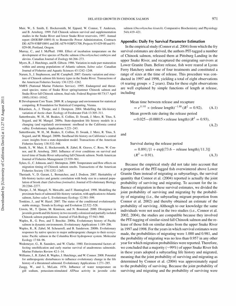
Appendix: Daily Fry Survival Parameter EstimationIn the empirical study (Connor et al. 2004) from which the fry

survival estimates are derived, the authors PIT-tagged a numberof Chinook salmon, released them at Pittsburg Landing in theupper Snake River, and recaptured the emigrating survivors atLower Granite Dam. Before release, fish were reared at LyonsFerry Hatchery under one of four treatments and constituted arange of sizes at the time of release. This procedure was con-ducted in 1997 and 1998, yielding a total of eight observations(4 rearing groups × 2 years). Data for these eight observationsare well explained by simple functions of length at release,including

Mean time between release and recapture

= e11.93 × (release length)−1.88 (R2 = 0.92), (A.1)

Mean growth rate during the release period

=0.025−(0.00015×release length) (R2 = 0.93),

(A.2)

and

Survival during the release period

= 0.891/{1 + exp[(73.6 − release length)/11.3]}(R2 = 0.91). (A.3)

Because the empirical study did not take into account thata proportion of the PIT-tagged fish overwintered above LowerGranite Dam instead of migrating as subyearlings, the survivalquantity that Connor et al. (2004) reported is actually the jointprobability of surviving and migrating. To account for the in-fluence of migration in these survival estimates, we divided thejoint probability of surviving and migrating by the probabil-ity of migrating (i.e., the subyearling migrant proportion fromConnor et al. 2002) and thereby obtained an estimate of theprobability of surviving. Although to our knowledge the sameindividuals were not used in the two studies (i.e., Connor et al.2002, 2004), the studies are compatible because they involvedthe PIT-tagging of similar-sized fall Chinook salmon and the re-lease of those fish on similar dates from the upper Snake Riverin 1997 and 1998. For the years in which survival estimates weremade, the probabilities of migrating were 1.000 and 0.981, andthe probability of migrating was no less than 0.957 in any otheryear for which migration probabilities were reported. Therefore,we concluded that a majority (∼99%) of upper Snake River fishin these years adopted a subyearling life history and migrated,meaning that the joint probability of surviving and migrating asdetermined by Connor et al. (2004) was approximately equalto the probability of surviving. Because the joint probability ofsurviving and migrating and the probability of surviving were

Dow

nloa

ded

by [

Uni

vers

ity o

f C

alif

orni

a D

avis

] at

11:

27 0

2 A

ugus

t 201

1

972 PERKINS AND JAGER

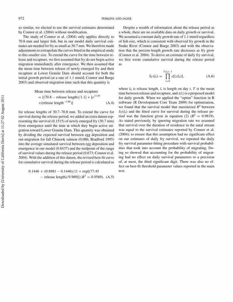
so similar, we elected to use the survival estimates determinedby Connor et al. (2004) without modification.

The study of Connor et al. (2004) only applies directly to70.8-mm and larger fish, but in our model daily survival esti-mates are needed for fry as small as 30.7 mm. We therefore madeadjustments to extrapolate the curves fitted in the empirical studyto this smaller size. To extend the curve for the time between re-lease and recapture, we first assumed that fry do not begin activemigration immediately after emergence. We then assumed thatthe mean time between release of newly emerged fry and theirrecapture at Lower Granite Dam should account for both theinitial growth period (at a rate of 1.1 mm/d; Connor and Burge2003) and observed migration time such that this quantity is

Mean time between release and recapture

= [(70.8 − release length)/1.1] + [e11.93

×(release length−1.88)] (A.4)

for release lengths of 30.7–70.8 mm. To extend the curve forsurvival during the release period, we added an extra datum rep-resenting the survival (0.1515) of newly emerged fry (30.7 mm)from emergence until the time at which they begin active mi-gration toward Lower Granite Dam. This quantity was obtainedby dividing the expected survival between egg deposition andout-migration for fall Chinook salmon (0.086; Bradford 1995)into the average simulated survival between egg deposition andemergence in our model (0.8437) and the midpoint of the rangeof survival values during the release period (0.673; Connor et al.2004). With the addition of this datum, the revised best-fit curvefor cumulative survival during the release period is calculated as

0.1446 + (0.8881 − 0.1446)/{1 + exp[(77.45

− release length)/9.969]} (R2 = 0.9569). (A.5)

Despite a wealth of information about the release period asa whole, there are no available data on daily growth or survival.We assumed a constant daily growth rate of 1.1 mm/d regardlessof fish size, which is consistent with observed fry growth in theSnake River (Connor and Burge 2003) and with the observa-tion that the percent-length growth rate decreases as fry grow(Connor et al. 2004). To derive an estimate of daily fry survival,we first wrote cumulative survival during the release periodas

ST (l0) =T (l0)−1∏

t=0

s[lt (l0)], (A.6)

where l0 is release length, lt is length on day t, T is the meantime between release and recapture, and s(lt) is a proposed modelfor daily growth. When we applied the “optim” function in Rsoftware (R Development Core Team 2009) for optimization,we found that the survival model that maximized R2 betweenST(l0) and the fitted curve for survival during the release pe-riod was the function given in equation (2) (R2 = 0.9819).As stated previously, by ignoring migration rate we assumedthat survival over the duration of residence in the natal streamwas equal to the survival estimates reported by Connor et al.(2004); to ensure that this assumption had no significant effecton our estimates of daily fry survival, we repeated the dailyfry survival parameter-fitting procedure with survival probabil-ities that took into account the probability of migrating. Do-ing so showed that accounting for the probability of migrat-ing had no effect on daily survival parameters to a precisionof, at most, the third significant digit. There was also no ef-fect on best-fit threshold parameter values reported in the maintext.

Dow

nloa

ded

by [

Uni

vers

ity o

f C

alif

orni

a D

avis

] at

11:

27 0

2 A

ugus

t 201

1