Earth Planets Space, 51, 1047–1058, 1999

Geoelectric structure beneath limestones of the Sao Francisco Basin, Brazil

J. M. Travassos1∗ and P. T. L. Menezes2

1CNPq-Observatorio Nacional, 20921-400 Rio de Janeiro, Brazil2FGEL/UERJ, 20559-900 Rio de Janeiro, Brazil

(Received November 30, 1998; Revised June 16, 1999; Accepted July 6, 1999)

A reconnaissance MT survey was conducted in the southern portion of the Sao Francisco Sedimentary Basin,Brazil, for mapping the subsurface structure. The objective was to provide a regional model and in helping to selectareas to be further surveyed with seismics. The data collected at seven EMAP-style spreads of 500 m, with anaverage spacing of 30 km. The field procedure allowed for the correction of statics and the production of 7 invertedmodels, smooth representations of the regional structure as seen below each site. A 2-D forward model tested andrefined the regional structure revealed by the inversions and yielded an earth composed of 4 main geologic units. A100 ohm.m limestone layer on the top of 20 ohm.m shales, followed by a 1000–200 ohm.m structured basement.Crustal resistivities do not change until reaching depths of more than 30 km. The model ends at a conductivehalf-space of 30 ohm.m. A suture zone between an orogenic belt and the Sao Francisco craton was modeled belowthe sedimentary section bringing its know limits 60 km to the east.

1. IntroductionElectromagnetic methods (EM) play a minor role in hy-

drocarbon exploration. They cannot yield a result with acomparable accuracy and spatial density as achieved by re-flection seismic. Yet they rank second to seismic methodsfor their resolution and depth of penetration. Moreover EMmethods are often well suited to exploration problems aris-ing due to high-velocity rocks (e.g., limestones, salt and vol-canics) or due to complex thrust and basin range geologicenvironments. In cases where high-velocity rocks are alsohighly resistive the contrast with the surrounding sedimentscan be more than one order of magnitude making those en-vironments good electrical targets.

EM methods can be used in a reconnaissance survey orin conjunction with seismics or other methods. The com-bined use of EM and seismic data can provide a differentinsight into exploration problems. In reconnaissance sur-veys EM methods can provide an inexpensive way of testinghypothesis before starting a seismic survey. Used in conjunc-tion with reflection seismics they may resolve ambiguities insome cases.

Among the EM techniques the magnetotelluric (MT)method has been widely used as an aid to petroleum explo-ration for several decades. The reliability of the MT methodhas improved due to advances in data acquisition (instru-mentation and field layout), data processing and 2-D/3-Dforward and inverse modeling codes. In terms of field layoutthe two most important advancements were the introductionof a remote reference (RR) to reduce the bias associated with

∗Formerly at Lamont-Doherty Observatory, Palisades, NY 10964,U.S.A.

Copy right c© The Society of Geomagnetism and Earth, Planetary and Space Sciences(SGEPSS); The Seismological Society of Japan; The Volcanological Society of Japan;The Geodetic Society of Japan; The Japanese Society for Planetary Sciences.

noisy magnetic field site (Gamble et al., 1979; Clarke et al.,1983) and the electromagnetic array profiling (EMAP) to re-move the ubiquitous static shift effects (Torres-Verdin andBostick, 1992a,b). Static effects are caused by the presenceof small-scale bodies in the near-surface. Static effects arenoticeable at periods where skin depths are much larger thanthe causative body. Those effects manifest themselves as ashift of apparent resistivity curves. Phase is not affected.

The most important element in impedance estimation wasthe introduction of the robust methods. The robust meth-ods can yield reliable impedance estimates in the presenceof a moderate number of violations of the assumptions ofGaussian distribution and in the presence of nonstationarynoise. Most of these methods are based on an iterativereweighted least squares scheme and may include data sub-stitution (Egbert and Booker, 1986; Chave et al., 1987; Chaveand Thomson, 1989, 1992; Larsen, 1989; Sutarno andVozoff, 1991; Larsen et al., 1996). In addition MT has highlydeveloped modeling capability that includes 3-D modeling(Dey and Morrison, 1979; Wannamaker et al., 1984, 1987;Wannamaker, 1991; Mackie et al., 1993).

The data shown in this work is part of a somewhat largerwork done for Petrobras, the Brazilian State Oil Company,on the Sao Francisco Basin, in a reconnaissance effort beforethe start of a seismic campaign. The interest on hydrocarbonexploration in the Proterozoic is recent in Brazil. It startedin the 70’s when gas was found in a water well. Three wellswere subsequently deployed based on a regional geologicmapping done in 1984–1986. The wells found gas (90%methane, 2% ethane and traces of propane) in a senile stageat 90 m depth (Braun et al., 1990). The source rocks have athickness of 500 m and the organic material is basically al-gae (Braun et al., 1990). The Sao Francisco Basin has aboutthe same age and geology as other oil producing basins else-

1047

1048 J. M. TRAVASSOS AND P. T. L. MENEZES: STRUCTURE BENEATH LIMESTONES

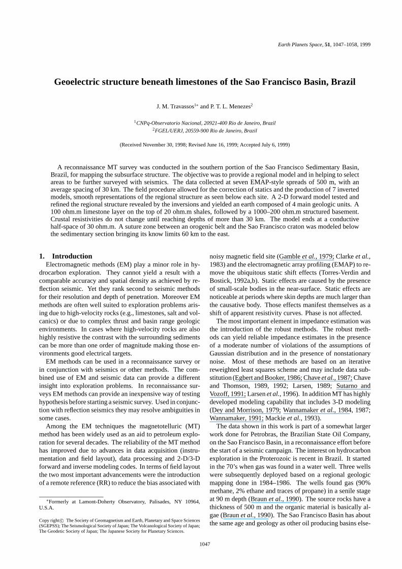
Fig. 1. Localization of the MT sites (5 to 11) superimposed on the Geological map of the survey area (CPRM, 1995). The black square in the inset showsthe localization of the mapped area in Brazil. J is the Joao Pinheiro fault and D is the Sao Domingos fault. L is a mapped magnetic lineament. Thegeological units traversed by the MT profile range from Quaternary clastic sediments (QP) and Mesosoic sandstones (Kmc) to the Proterozoic arkosesand limestones of the Bambui Group (PStm and PSb), stopping short of the quartzites of the Cabral Range.

where in the world, such as Irkutsk (Russia) and Officer andAmadeus (Australia) (Murray et al., 1980). A main differ-ence here is the absence of evaporite sequences in the SaoFrancisco Basin. The geophysical knowledge of the basin isscarce and scattered. A review of the work done in the areacan be found in the literature (Ussami, 1993). No other geo-physical data are available in the area covered in this work.But elsewhere in the basin there are some gravimetric data(Blitzkow et al., 1979; Lesquer et al., 1981; Assumpcao etal., 1984; Ussami, 1986; Ortu, 1990) and refraction seismics(Knize et al., 1984; Berrocal et al., 1989). Accordingly tothose last two works the Moho is estimated to be at 43 km. Aseismic tomography study done just over 300 km due southof the studied area has estimated the basement of the basin tolie at 2.8 km, below the Brasilia mobile belt (Marchioreto andAssumpcao, 1997). There are many isolated aeromagneticsurveys on the basin but no regional interpretation that con-solidates the information (Ussami, 1993). There is anotherMT survey about 150 km north of the survey area where theinterpretation was based entirely on 1D inversions (Porsaniand Fontes, 1993).

2. Survey Area2.1 Geology

The foreland Sao Francisco Basin is located in the north-eastern part of Brazil spanning over 216,000 km2. Its main

sedimentary group is the upper Proterozoic Bambui Group, asequence laid on a carbonate platform sculptured onto a com-plex basement (Braun, 1982). Basement rocks are mostlyArchean migmatites and granitoids of the Sao Francisco cra-ton and middle Proterozoic highly folded metassediments ofthe Arari (siltstones and quartzites) and Espinhaco(quartzites) supergroups. The Bambui Group covers mostof the Sao Francisco craton and is affected by the tectonic-magmatic events associated with the Brazilian orogeny (650–550 Ma). The Bambui Group is divided into the upper TresMarias formation (arkoses) and Paraopeba subgroup (car-bonates).

Figure 1 shows a geologic map of the survey region on a1:2,500,000 scale (CPRM, 1995). The profile traverses overQuaternary clastic sediments, late Proterozoic arkoses andlimestones of the Bambui Group, stopping short of the mid-dle Proterozoic quartzites of the Cabral Range. The BambuiGroup displays on its western limit a highly folded domainbounded by a subvertical reverse fault: the Sao Domingosfault (see Fig. 1). From that fault to the east the subsurfaceis flat-layered except for some confined domains which be-come more frequent to the east and southeast of Fig. 1. Thesefolds remain less intense than to the west. Fractures basicallygroup in two systems: NNW and NE. The western side ismore fractured and displays Appalachian-like folding belts.Those faults display high dip angles and a rectilinear signa-

J. M. TRAVASSOS AND P. T. L. MENEZES: STRUCTURE BENEATH LIMESTONES 1049

ture due to a compressive stress regime (Braun, 1982). Thisstress regime has actuated since the beginning of the Bambuideposition, due to stress on the craton as represented by theProterozoic heavily folded Brasilia mobile belt (Valeriano,1992). The present knowledge on the basin indicates thatthe deposition of the Bambui Group occurred on a forelandbasin with origin in the tectonic buildup that resulted dur-ing from the compressive stress regime represented by theBrasilia mobile belt (Proterozoic) on the Sao Francisco cra-ton (Archean) (Thomaz et al., 1998).2.2 Site location and layout

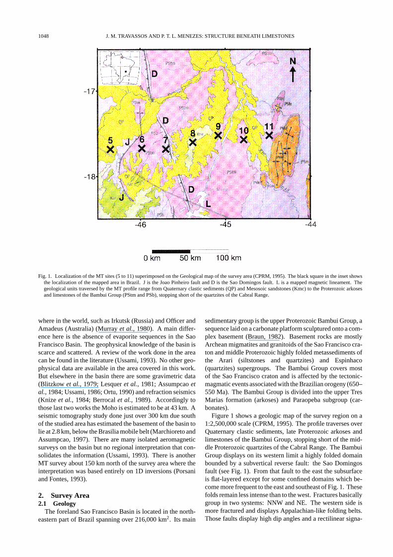
The data set of this work was collected along a 207 kmlong EW MT profile as seen in Fig. 1. The profile wasdesigned to be perpendicular to the known geological strike.The 7 remote referenced sites were obtained with equipmentmanufactured by EMI Inc. All sites were recorded broadbandcovering the range from 103 to 10−3 Hz. Sites were spaced 30km on average. A remote site was deployed at a distance of20–30 km away from any given site. Each site was laid out asa EMAP-like spread with 5 contiguous dipoles along profiledirection, namely the x-direction, and 1 perpendicular dipolealong the y-direction. All dipoles are 100 m long, renderinga 500 m long EMAP spread at each location. Each dipolealong the x-direction is numbered sequentially from west toeast as: 1, . . . , 5. The y-dipole is deployed somewhere alongthe spread. The magnetic field vertical component was notrecorded because all available channels were used to recordthe horizontal field components. Figure 2 shows the fieldlayout used for site 11: the y-dipole was deployed betweenx-dipoles 2 and 3. Assuming the electric field along the y-direction does not vary too much each setup is equivalent to5 contiguous remote reference sites. Each of the 5 subsites isobtained combining a particular x-dipole, from 1 to 5, withthe y-dipole. Note the whole profile is then equivalent to35 remote reference sites with uneven spacing. Infield dataprocessing (for single site only) allowed an efficient dataquality assessment. The production rate averaged 1.3 sites aday for a crew of 4–5 people.

3. Data ProcessingAt each site n, n = 5, . . . , 11, the coupling between the

local electromagnetic field components is given by[E (i,n)

x

E (n)y

]=

[Z (i,n)

xx Z (i,n)xy

Z (n)yx Z (n)

yy

]·[

H (n)x

H (n)y

](1)

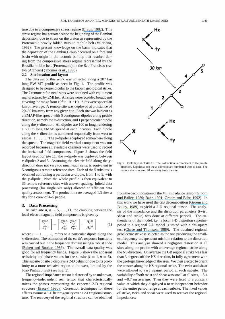
where i = 1, . . . , 5, refers to a particular dipole along thex-direction. The estimation of the earth’s response functionswas carried out in the frequency domain using a robust code(Egbert and Booker, 1986). The overall data quality wasgood for all frequency bands. Figure 3 shows the apparentresistivity and phase values for the subsite (i = 1, n = 6).This subsite of site 6 displays a 2-D behavior due to its prox-imity to a more resistive region to the west, limited by theJoao Pinheiro fault (see Fig. 1).

The regional impedance tensor is distorted by an unknown,frequency-independent real tensor that characteristicallymixes the phases representing the expected 2-D regionalstructure (Jiracek, 1990). Correction techniques for theseeffects assume a 3-D heterogeneity over a 2-D regional struc-ture. The recovery of the regional structure can be obtained

Fig. 2. Field layout of site 11. The x-direction is coincident to the profiledirection. Dipoles along the x-direction are numbered west to east. Theremote site is located 30 km away from the site.

from the decomposition of the MT impedance tensor (Groomand Bailey, 1989; Bahr, 1991; Groom and Bahr, 1992). Inthis work we have used the GB decomposition (Groom andBailey, 1989) to yield a 2-D regional tensor. The analy-sis of the impedance and the distortion parameters (twist,shear and strike) was done at different periods. The au-thenticity of the model, i.e., a local 3-D distortion superim-posed to a regional 2-D model is tested with a chi-squaretest (Chave and Thomson, 1989). The obtained regionalgeoelectric strike is selected as the one producing the small-est frequency-independent misfit in relation to the distortionmodel. This analysis showed a negligible distortion at allsites along the profile with an average regional strike alongthe NS direction. On average the GB regional strike was lessthan 3 degrees off the NS direction, in fully agreement withthe geologic knowledge of the area. We then elected to orientthe tensors along the NS regional strike. The twist and shearwere allowed to vary against period at each subsite. Thevariability of both twist and shear was small at all sites, −3.4and −0.7 on average. Then they were fixed to a constantvalue at which they displayed a near independent behaviorfor the entire period range at each subsite. The fixed valuesof strike, twist and shear were used to recover the regionalimpedances.

1050 J. M. TRAVASSOS AND P. T. L. MENEZES: STRUCTURE BENEATH LIMESTONES

Fig. 3. Apparent resistivity and phase at subsite (i = 1, n = 6) of site 6. TE estimates are shown as circles and the TM as squares. Error bars correspondto a 95% confidence interval.

4. 2-D Inversion and Static CorrectionThe following analysis is done on the recovered GB 2-D

regional impedances obtained as described in the last sec-tion. At this point the phases express the regional model butboth site gain and anisotropy may still affect the resistivityvalues. There are a number of ways to correct for the staticshift phenomenon whereas anisotropy can be solved throughmodeling. The static shift may be corrected if one has a suf-ficiently dense MT spatial coverage: the EMAP techniqueis designed to deal with such distortion (Torres-Verdin andBostick, 1992a,b). Sometimes even isolated sites can be usedas long as all sites resolve at least one regional feature (Jones,1988). In this case apparent resistivity curve shifting (Jones,1988) and/or an inversion effort with the gain factors freeat each site may be used (Chouteau et al., 1997). Simplecurve shifting assumes no intrinsic anisotropy. Other way

to correct for static shift effects is to resort to independentgeophysical data, e.g., electrical or electromagnetic field data(Pellerin and Hohmann, 1990; Chouteau et al., 1997).

None of those are applicable to the present data set. Sitesare spaced 30 km on average, too isolated to allow the cor-rection of static shift using the data from neighboring sites orthe estimation of a reference value for the apparent resistivitycurves. On the other hand there is no independent data either.EMAP spatial filtering (Torres-Verdin and Bostick, 1992b)cannot be used within the spreads as depths of interest arewell over their lateral dimension.

In this work we take advantage of the continuous fieldlayout of 5 subsites at each site to correct for static distortions.We assume that the E-polarization electric field (Ey) does notchange too much along a spread to allow the use of expression(1), i.e., the equivalence to 5 contiguous remote reference MT

J. M. TRAVASSOS AND P. T. L. MENEZES: STRUCTURE BENEATH LIMESTONES 1051

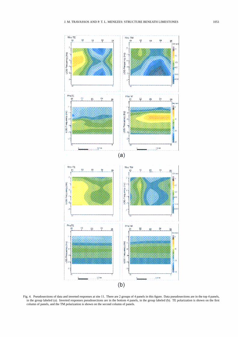
Fig. 4. Pseudosections of data and inverted responses at site 11. There are 2 groups of 4 panels in this figure. Data pseudosections are in the top 4 panels,in the group labeled (a). Inverted responses pseudosections are in the bottom 4 panels, in the group labeled (b). TE polarization is shown on the firstcolumn of panels, and the TM polarization is shown on the second column of panels.

1052 J. M. TRAVASSOS AND P. T. L. MENEZES: STRUCTURE BENEATH LIMESTONES

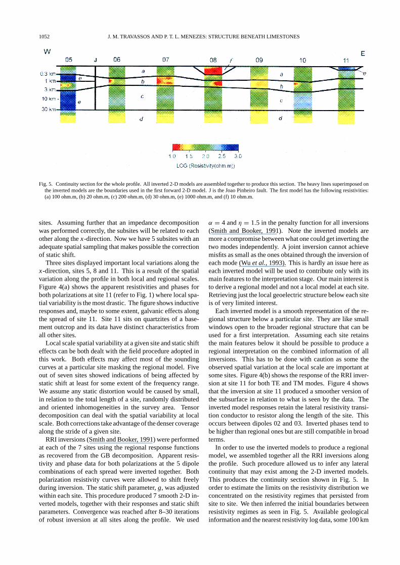
Fig. 5. Continuity section for the whole profile. All inverted 2-D models are assembled together to produce this section. The heavy lines superimposed onthe inverted models are the boundaries used in the first forward 2-D model. J is the Joao Pinheiro fault. The first model has the following resistivities:(a) 100 ohm.m, (b) 20 ohm.m, (c) 200 ohm.m, (d) 30 ohm.m, (e) 1000 ohm.m, and (f) 10 ohm.m.

sites. Assuming further that an impedance decompositionwas performed correctly, the subsites will be related to eachother along the x-direction. Now we have 5 subsites with anadequate spatial sampling that makes possible the correctionof static shift.

Three sites displayed important local variations along thex-direction, sites 5, 8 and 11. This is a result of the spatialvariation along the profile in both local and regional scales.Figure 4(a) shows the apparent resistivities and phases forboth polarizations at site 11 (refer to Fig. 1) where local spa-tial variability is the most drastic. The figure shows inductiveresponses and, maybe to some extent, galvanic effects alongthe spread of site 11. Site 11 sits on quartzites of a base-ment outcrop and its data have distinct characteristics fromall other sites.

Local scale spatial variability at a given site and static shifteffects can be both dealt with the field procedure adopted inthis work. Both effects may affect most of the soundingcurves at a particular site masking the regional model. Fiveout of seven sites showed indications of being affected bystatic shift at least for some extent of the frequency range.We assume any static distortion would be caused by small,in relation to the total length of a site, randomly distributedand oriented inhomogeneities in the survey area. Tensordecomposition can deal with the spatial variability at localscale. Both corrections take advantage of the denser coveragealong the stride of a given site.

RRI inversions (Smith and Booker, 1991) were performedat each of the 7 sites using the regional response functionsas recovered from the GB decomposition. Apparent resis-tivity and phase data for both polarizations at the 5 dipolecombinations of each spread were inverted together. Bothpolarization resistivity curves were allowed to shift freelyduring inversion. The static shift parameter, g, was adjustedwithin each site. This procedure produced 7 smooth 2-D in-verted models, together with their responses and static shiftparameters. Convergence was reached after 8–30 iterationsof robust inversion at all sites along the profile. We used

α = 4 and η = 1.5 in the penalty function for all inversions(Smith and Booker, 1991). Note the inverted models aremore a compromise between what one could get inverting thetwo modes independently. A joint inversion cannot achievemisfits as small as the ones obtained through the inversion ofeach mode (Wu et al., 1993). This is hardly an issue here aseach inverted model will be used to contribute only with itsmain features to the interpretation stage. Our main interest isto derive a regional model and not a local model at each site.Retrieving just the local geoelectric structure below each siteis of very limited interest.

Each inverted model is a smooth representation of the re-gional structure below a particular site. They are like smallwindows open to the broader regional structure that can beused for a first interpretation. Assuming each site retainsthe main features below it should be possible to produce aregional interpretation on the combined information of allinversions. This has to be done with caution as some theobserved spatial variation at the local scale are important atsome sites. Figure 4(b) shows the response of the RRI inver-sion at site 11 for both TE and TM modes. Figure 4 showsthat the inversion at site 11 produced a smoother version ofthe subsurface in relation to what is seen by the data. Theinverted model responses retain the lateral resistivity transi-tion conductor to resistor along the length of the site. Thisoccurs between dipoles 02 and 03. Inverted phases tend tobe higher than regional ones but are still compatible in broadterms.

In order to use the inverted models to produce a regionalmodel, we assembled together all the RRI inversions alongthe profile. Such procedure allowed us to infer any lateralcontinuity that may exist among the 2-D inverted models.This produces the continuity section shown in Fig. 5. Inorder to estimate the limits on the resistivity distribution weconcentrated on the resistivity regimes that persisted fromsite to site. We then inferred the initial boundaries betweenresistivity regimes as seen in Fig. 5. Available geologicalinformation and the nearest resistivity log data, some 100 km

J. M. TRAVASSOS AND P. T. L. MENEZES: STRUCTURE BENEATH LIMESTONES 1053

north of the profile were used to aid in this task. It is assumedhere that the boundaries inferred in the continuity section canreproduce the main regional, i.e., long wavelength, featuresalong the profile.

Based on the model shown in Fig. 5 the layered structure ofthe basin is composed of 4 main geoelectric units. A resistorunit of 100 ohm.m on the top of a conductor of 20 ohm.m. Aresistive zone of 1000–200 ohm.m follows those units. Thisresistive zone extends down to about 30 km where there isa transition to a conductor of 30 ohm.m. That transition isparticularly clear at sites 05 and 10. Three sites display amore involved structure: 05, 08 and 11. Site 05 sits on amore resistive region of 1000 ohm.m, probably associated tothe Brasilia Mobile Belt rocks. The limit between this highresistor and the more conductive rocks to the east is inferredas the Joao Pinheiro fault. The shallow conductor at site 08is probably associated to mapped sandstones. The shallowresistor at site 11 are quartzites that were locally mapped. Re-sistivity regimes and their boundaries show variations fromsite to site. Therefore the adopted values depend on how welook at the smooth transitions of the inverted models. Thisis as far as we can go with the first model shown in Fig. 5.

5. 2-D ModelingThe initial model shown in Fig. 5 can be regarded as a first

approximation to recover the regional structure based on the2-D inversions and on the limited independent geologicaland geophysical data available. The regional features of thatmodel can be further tested and eventually refined with 2-Dforward modeling. The modeling exercise was done usinga finite element algorithm (Wannamaker et al., 1987). Thevalidity and sensibility of our model can be assessed compar-ing model responses to the observed data. The objective ofthe modeling exercise was to produce a minimum structurethat is still able to explain the regional impedances. The for-ward model will necessarily incorporate both regional (longwavelength) and more localized features eventually neededto locally improve the fit of model responses to the data. Inparticular shorter wavelength features as the shallow conduc-tor at site 8 and the resistor below site 11 were tentativelyincluded in the initial forward model.

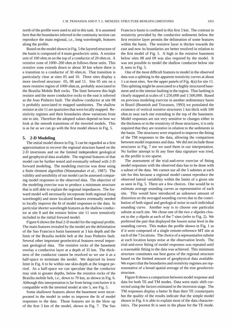
Figure 6 shows the final 2-D model for the regional profile.The main features revealed by the model are the delimitationof the Sao Francisco basin basement at 3 km depth and thelimit of the Brasilia mobile belt at the Joao Pinheiro fault.Several other important geoelectrical features reveal impor-tant geological data. The resistive rocks of the basementoverlay a conductive layer at a depth of 35 km. The thick-ness of the conductor cannot be resolved so we use it as ahalf-space to terminate the model. We depicted its lowerlimit in Fig. 6 to be within one skin-depth at the longest pe-riod. As a half-space we can speculate that the conductormay sink to greater depths, below the resistive rocks of theBrasilia mobile belt, i.e., down to 70 km, as shown in Fig. 6.Although this interpretation is far from being conclusive it iscompatible with the inverted model at site 5, see Fig. 5.

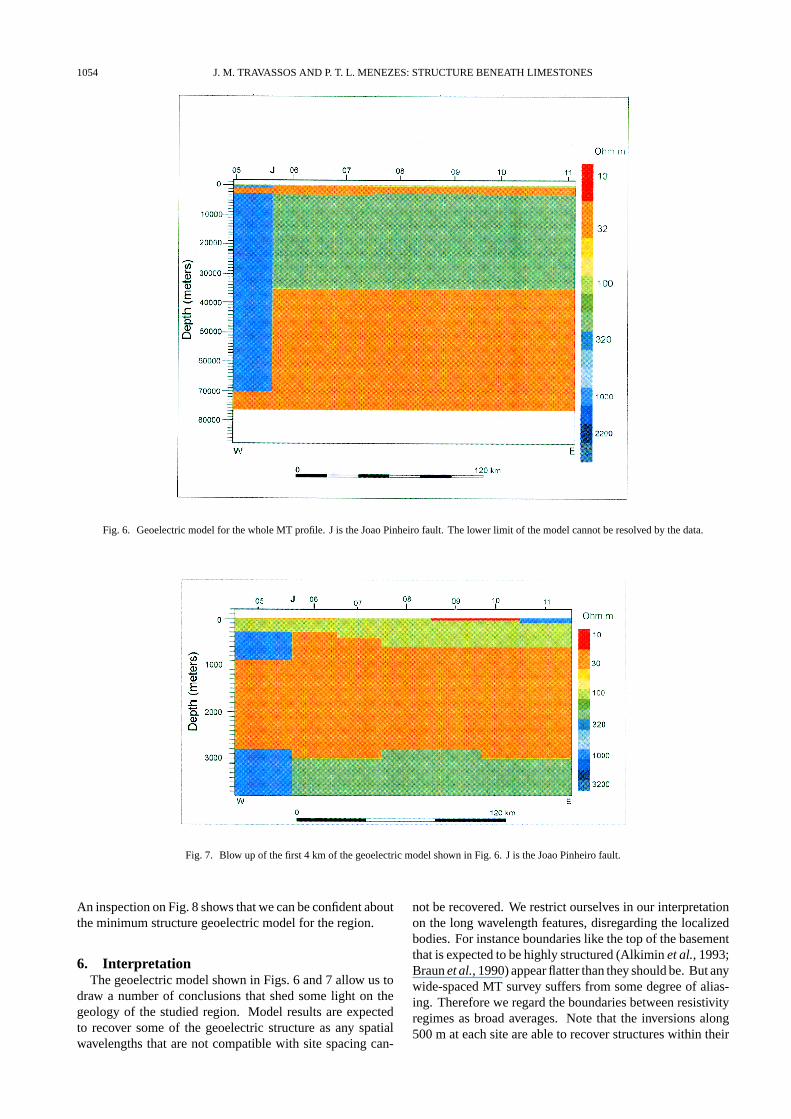
Some shallower features above the basement were incor-porated in the model in order to improve the fit of modelresponses to the data. Those features are in the blow upof the first 3 km of the model, shown in Fig. 7. The Sao

Francisco basin is confined in this first 3 km. The contrast inresistivity provided by the conductive sediments below thefirst resistive layer permits the delineation of some featureswithin the basin. The resistive layer is thicker towards theeast and now its boundaries are better resolved in relation tothe first model of Fig. 5. A high in the resistive basementbelow sites 08 and 09 was also required by the model. Itwas not possible to model the shallow conductor below site8, seen in Fig. 5.

One of the most difficult features to model in the observeddata was a splitting in the apparent resistivity curves at about1 s at most sites. See the upper panels of Fig. 4(a) for site 11.This splitting might be associated to a highly structured base-ment and to the intense faulting in the region. That faulting isclearly mapped at scales of 1:250,000 and 1:500,000. Basedon previous modeling exercise in another sedimentary basinin Brazil (Beamish and Travassos, 1993) we postulated theexistence of vertical resistive structures 1 km thick with 100ohm.m near each site extending to the top of the basement.Model responses are not very sensitive to changes either inthe thickness or in the resistivity of those structures, it is onlyrequired that they are resistive in relation to the sediments inthe basin. The structures were required to improve the fittingof the TM responses to the data, allowing the comparisonbetween model responses and data. We did not include thosestructures in Fig. 7 nor we used them in our interpretation.No further attempt to fit any finer data signature was tried,as the profile is too sparse.

The assessment of the trial-and-error exercise of fittingmodel responses with the observed data has to be done witha subset of the data. We cannot use all the 5 subsites at eachsite for this because a regional model cannot reproduce theobserved lateral variability within the limits of a given siteas seen in Fig. 5. There are a few choices. One would be toestimate average sounding curves as representative of eachsite. This would have introduced an unknown amount ofdistortion on the averaged sounding curves due to the contri-bution of both signal and geological noise in each individualsounding curve. Another way is to choose one particularsubsite at each site. We chose one of the two x-dipoles clos-est to the y-dipole at each of the 7 sites (refer to Fig. 2). Wepreferred the pair that displayed the lowest noise level in thesounding curves. This makes the profile shown in Fig. 1 asif it were composed of a single remote-reference MT site ateach of the 7 locations. The choice of a representative subsiteat each location keeps noise at the observation levels. Thetrial-and-error fitting of model responses was repeated untila reasonable fitting to the data was achieved. This minimumstructure constitutes our best guess of the regional structurebased on the limited amount of geophysical data available.We expect that the boundaries and resistivity regimes are rep-resentative of a broad spatial average of the true geoelectricstructure.

Figure 8 shows a comparison between model response anddata for both TE and TM modes. Data were static shift cor-rected using the factors estimated in the inversion stage. TheTM responses display a better fit than their TE counterpartsbut the quality of the results indicate that the simple modelshown in Fig. 6 is able to explain most of the data character-istics. The poorest fit is seen in the phase for the TE mode.

1054 J. M. TRAVASSOS AND P. T. L. MENEZES: STRUCTURE BENEATH LIMESTONES

Fig. 6. Geoelectric model for the whole MT profile. J is the Joao Pinheiro fault. The lower limit of the model cannot be resolved by the data.

Fig. 7. Blow up of the first 4 km of the geoelectric model shown in Fig. 6. J is the Joao Pinheiro fault.

An inspection on Fig. 8 shows that we can be confident aboutthe minimum structure geoelectric model for the region.

6. InterpretationThe geoelectric model shown in Figs. 6 and 7 allow us to

draw a number of conclusions that shed some light on thegeology of the studied region. Model results are expectedto recover some of the geoelectric structure as any spatialwavelengths that are not compatible with site spacing can-

not be recovered. We restrict ourselves in our interpretationon the long wavelength features, disregarding the localizedbodies. For instance boundaries like the top of the basementthat is expected to be highly structured (Alkimin et al., 1993;Braun et al., 1990) appear flatter than they should be. But anywide-spaced MT survey suffers from some degree of alias-ing. Therefore we regard the boundaries between resistivityregimes as broad averages. Note that the inversions along500 m at each site are able to recover structures within their

J. M. TRAVASSOS AND P. T. L. MENEZES: STRUCTURE BENEATH LIMESTONES 1055

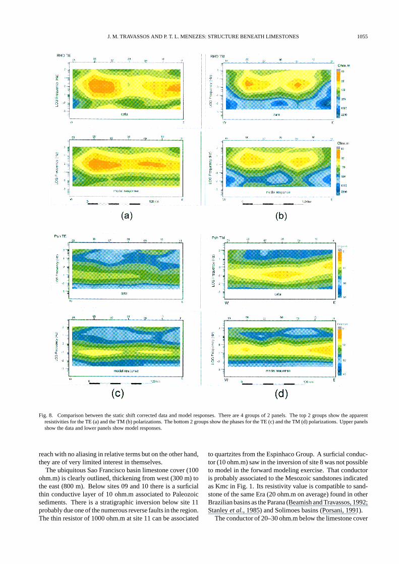
Fig. 8. Comparison between the static shift corrected data and model responses. There are 4 groups of 2 panels. The top 2 groups show the apparentresistivities for the TE (a) and the TM (b) polarizations. The bottom 2 groups show the phases for the TE (c) and the TM (d) polarizations. Upper panelsshow the data and lower panels show model responses.

reach with no aliasing in relative terms but on the other hand,they are of very limited interest in themselves.

The ubiquitous Sao Francisco basin limestone cover (100ohm.m) is clearly outlined, thickening from west (300 m) tothe east (800 m). Below sites 09 and 10 there is a surficialthin conductive layer of 10 ohm.m associated to Paleozoicsediments. There is a stratigraphic inversion below site 11probably due one of the numerous reverse faults in the region.The thin resistor of 1000 ohm.m at site 11 can be associated

to quartzites from the Espinhaco Group. A surficial conduc-tor (10 ohm.m) saw in the inversion of site 8 was not possibleto model in the forward modeling exercise. That conductoris probably associated to the Mesozoic sandstones indicatedas Kmc in Fig. 1. Its resistivity value is compatible to sand-stone of the same Era (20 ohm.m on average) found in otherBrazilian basins as the Parana (Beamish and Travassos, 1992;Stanley et al., 1985) and Solimoes basins (Porsani, 1991).

The conductor of 20–30 ohm.m below the limestone cover

1056 J. M. TRAVASSOS AND P. T. L. MENEZES: STRUCTURE BENEATH LIMESTONES

can be interpreted as the pelitic units of the basin. Thisconclusion is based on the data from a stratigraphic well 100km north of the profile. The well cuts a section of shalesand siltites of more than 1 km of thickness below 300 m oflimestones (Braun et al., 1990). Before this work the wholeBambui Group was estimated to reach up to 2 km in thicknessin the deepest portions of the basin (Braun et al., 1990). Herewe found the electrical basement at 2.8–3.0 km, 1 km deeperthan the previous estimates based on geological data. Ourestimate is in accordance with a recent seismic tomographystudy that estimated the basement of the basin to lie at 2.8 kmjust over 300 km due south of the studied area (Marchioretoand Assumpcao, 1997).

A high in the basement was modeled below sites 8 and9. It has possibly the same origin as another high 70 km tothe south identified from gravity data (Lesquer et al., 1981).That structure was later identified as the Sete Lagoas High(SLH) (D’Arrigo et al., 1995). A flexural model for thesouthern Sao Francisco craton (Ortu, 1990) showed that theSLH is a result of the load originated during the installationof the Brasilia mobile belt at the western limit of the craton.The high found below sites 8 and 9 probably results fromthat same mechanism. Under this mechanism the basementrocks would be pushed upwards due to the compressive stressregime. The intense faulting in the region is a result of thatsame mechanism.

The electrical basement is not uniform being more resistiveon its western end, 1000 ohm.m, than elsewhere where it hasresistivity of 200 ohm.m. The basement rocks extend togreater depths to about 35 km; less than 10 km short of theMoho at 43 km (Knize et al., 1984; Berrocal et al., 1989).At the resistive western end the resistive rocks extend downto 70 km, ending at the conductive half-space of 30 ohm.m.Model responses from those depths at the western end areright at the limit of our period range. But there is someindication that the conductor may sink below the resistiverocks, well beyond the known Moho. This is compatible tothe inversion of site 5 as it shows the conductor below theresistive rocks.

Another result of this work is the localization of the con-tact between two crustal blocks: the Brasilia mobile beltand the Sao Francisco craton. That contact is buried belowmetassediments of the Bambui Group at the Joao Pinheirofault, indicated with a J in Fig. 1. The Brasilia mobile beltoutcrops 60 km west of site 5 (Alkimin et al., 1993). Priorto this work that suture zone was thought to lie along the SaoDomingos fault (Thomaz Filho, personal communication,1998), indicated with a D in Fig. 1, as it is a limit betweenthe folded and unfolded (less affected by orogenesis) BambuiGroup.

Apart from the lateral resistivity contrast the modeled up-per crust is electrically homogeneous throughout with noevidence of crustal conductors in it. The contact betweenthe resistive upper crust and the lower crust/upper mantleconductor of 30 ohm.m lies at the limit of the period range;its thickness cannot be resolved within the frequency range.Notwithstanding this lack of resolution the data does requirethe presence of a strong conductor at lower crust depths.

Crustal conductors are very common throughout theearth’s crust (Haak and Hutton, 1986; Schwarz, 1990;

Brown, 1994; Haak et al., 1996). Their presence was mod-eled in other Brazilian regions as below the Parana basin(Stanley et al., 1985; Beamish and Travassos, 1992) andthe Solimoes Basin (Porsani, 1991). Otherwise crustal re-sistivities of 200–1000 ohm.m are compatible with the fig-ures found in other cratonic regions (Haak and Hutton, 1986;Hyndman and Shearer, 1989; Brown, 1994). Moreover con-ductors situated below a resistive and homogeneous upperand medium crust with resistivities compatible to ours havebeen reported extensively in the literature (Simpson, 1998)and are usually explained as a result of the presence of salinefluids, sulfide and graphite.

7. ConclusionsThis work presents the results from a reconnaissance MT

survey in the southern portion of the Sao Francisco sedimen-tary basin, Brazil. Data were collected along a profile 207km long, at seven 500 m long EMAP-style spreads. Thisapproach allowed for the correction of the static shift dis-tortion and produced 7 2-D independently inverted models.Each model is a 500 m across smooth representation of theregional structure as seen below each site. Those 2-D modelswere then assembled together in a section to infer any lateralcontinuity that may exist among them thus producing a firstregional model. It is assumed that the continuity section canapproximately reproduce the long wavelength features alongthe profile. Shorter wavelength regional features cannot beadequately reproduced due to site spacing.

We used the model inferred with the continuity sectionas a first model in a forward 2-D modeling exercise. Theobjective of the forward modeling was to test and refine thefirst model. The final 2-D outlined the great sedimentaryunits and the electrical basement of the Basin. The lowerlimit for the basin limestone cover (100 ohm.m) was clearlydelineated, thickening from west (300 m) to the east (800 m).A surficial thin conductive layer of 10 ohm.m associated toPaleozoic sediments was delineated below sites 09 and 10.A surficial conductor of 10 ohm.m at site 8 was associated tothe Mesozoic sandstones. The conductor of 20–30 ohm.mbelow the limestone cover was interpreted as the pelitic unitsof the basin.

The basement was found at 2.8–3 km and a high was delin-eated below sites 8 and 9. At the more resistive western endof the profile the resistive rocks extend down to 70 km. The 2-D model ends at a conductive half-space of 30 ohm.m. Thecrustal contact was interpreted as the suture zone betweentwo distinct crustal blocks: the lower Proterozoic rocks ofthe Brasilia mobile belt and the Archean rocks of the SaoFrancisco craton. The contact between these two tectonicunits occurs at the Joao Pinheiro Fault extending eastwardsthe previous knowledge by more than 60 km. Moreover theBrasilia mobile belt crustal block may extends well beyondthe previously known Moho in contrast to the craton to theeast ending just short of it.

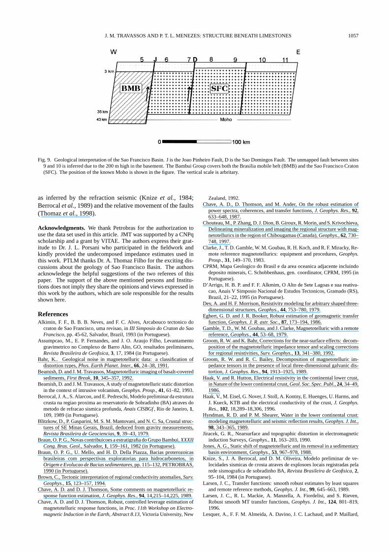
Figure 9 summarizes the geological interpretation basedon the 2-D model of Figs. 5, 6 and 7 as well as on a recentgeological model (Thomaz et al., 1998). The Joao Pinheirofault is the contact between the lower Proterozoic rocks ofthe Brasilia mobile belt and the Archean rocks of the SaoFrancisco craton. Figure 9 includes the position of the Moho

J. M. TRAVASSOS AND P. T. L. MENEZES: STRUCTURE BENEATH LIMESTONES 1057

Fig. 9. Geological interpretation of the Sao Francisco Basin. J is the Joao Pinheiro Fault, D is the Sao Domingos Fault. The unmapped fault between sites9 and 10 is inferred due to the 200 m high in the basement. The Bambui Group covers both the Brasilia mobile belt (BMB) and the Sao Francisco Craton(SFC). The position of the known Moho is shown in the figure. The vertical scale is arbritary.

as inferred by the refraction seismic (Knize et al., 1984;Berrocal et al., 1989) and the relative movement of the faults(Thomaz et al., 1998).

Acknowledgments. We thank Petrobras for the authorization touse the data set used in this article. JMT was supported by a CNPqscholarship and a grant by VITAE. The authors express their grat-itude to Dr. J. L. Porsani who participated in the fieldwork andkindly provided the undecomposed impedance estimates used inthis work. PTLM thanks Dr. A. Thomaz Filho for the exciting dis-cussions about the geology of Sao Francisco Basin. The authorsacknowledege the helpful suggestions of the two referees of thispaper. The support of the above mentioned persons and Institu-tions does not imply they share the opinions and views expressed inthis work by the authors, which are sole responsible for the resultsshown here.

ReferencesAlkimin, F. F., B. B. B. Neves, and F. C. Alves, Arcabouco tectonico do

craton de Sao Francisco, uma revisao, in III Simposio do Craton do SaoFrancisco, pp. 45-62, Salvador, Brazil, 1993 (in Portuguese).

Assumpcao, M., E. P. Fernandes, and J. O. Araujo Filho, Levantamentogravimetrico no Complexo de Barro Alto, GO, resultados preliminares,Revista Brasileira de Geofisica, 3, 17, 1984 (in Portuguese).

Bahr, K.. Geological noise in magnetotelluric data: a classification ofdistortion types, Phys. Earth Planet. Inter., 66, 24–38, 1991.

Beamish, D. and J. M. Travassos, Magnetotelluric imaging of basalt-coveredsediments, First Break, 10, 345–357, 1992.

Beamish, D. and J. M. Travassos, A study of magnetotelluric static distortionin the context of intrusive volcanism, Geophys. Prosp., 41, 61–82, 1993.

Berrocal, J. A., S. Alarcon, and E. Pedreschi, Modelo preliminar da estruturacrusta na regiao proxima ao reservatorio de Sobradinho (BA) atraves dometodo de refracao sismica profunda, Anais CISBGf , Rio de Janeiro, 1,109, 1989 (in Portuguese).

Blitzkow, D., P. Gasparini, M. S. M. Mantovani, and N. C. Sa, Crustal struc-tures of SE Minas Gerais, Brazil, deduced from gravity measurements,Revista Brasileira de Geociencias, 9, 39–43, 1979.

Braun, O. P. G., Novas contribuicoes a estratigrafia do Grupo Bambui, XXXIICong. Bras. Geol., Salvador, 1, 159–161, 1982 (in Portuguese).

Braun, O. P. G., U. Mello, and H. D. Della Piazza, Bacias proterozoicasbrasileiras com perspectivas exploratorias para hidrocarbonetos, inOrigem e Evolucao de Bacias sedimentares, pp. 115–132, PETROBRAS,1990 (in Portuguese).

Brown, C., Tectonic interpretation of regional conductivity anomalies, Surv.Geophys., 15, 123–157, 1994.

Chave, A. D. and D. J. Thomson, Some comments on magnetotelluric re-sponse function estimation, J. Geophys. Res., 94, 14,215–14,225, 1989.

Chave, A. D. and D. J. Thomson, Robust, controlled leverage estimation ofmagnetotelluric response functions, in Proc. 11th Workshop on Electro-magnetic Induction in the Earth, Abstract 8.13, Victoria University, New

Zealand, 1992.Chave, A. D., D. Thomson, and M. Ander, On the robust estimation of

power spectra, coherences, and transfer functions, J. Geophys. Res., 92,633–648, 1987.

Chouteau, M., P. Zhang, D. J. Dion, B. Giroux, R. Morin, and S. Krivochieva,Delineating mineralization and imaging the regional structure with mag-netotellurics in the region of Chibougamau (Canada), Geophys., 62, 730–748, 1997.

Clarke, J., T. D. Gamble, W. M. Goubau, R. H. Koch, and R. F. Miracky, Re-mote reference magnetotellurics: equipment and procedures, Geophys.Prosp., 31, 149–170, 1983.

CPRM, Mapa Geologico do Brasil e da area oceanica adjacente incluindodeposito minerais, C. Schobbenhaus, gen. coordinator, CPRM, 1995 (inPortuguese).

D’Arrigo, H. B. P. and F. F. Alkmim, O Alto de Sete Lagoas e sua reativa-cao, Anais V Simposio Nacional de Estudos Tectonicos, Gramado (RS),Brazil, 21–22, 1995 (in Portuguese).

Dey, A. and H. F. Morrison, Resistivity modeling for arbitrary shaped three-dimensional structures, Geophys., 44, 753–780, 1979.

Egbert, G. D. and J. R. Booker, Robust estimation of geomagnetic transferfunction, Geophys. J. R. astr. Soc., 87, 173–194, 1986.

Gamble, T. D., W. M. Goubau, and J. Clarke, Magnetotelluric with a remotereference, Geophys., 44, 53–68, 1979.

Groom, R. W. and K. Bahr, Corrections for the near-surface effects: decom-position of the magnetotelluric impedance tensor and scaling correctionsfor regional resistivities, Surv. Geophys., 13, 341–380, 1992.

Groom, R. W. and R. C. Bailey, Decomposition of magnetotelluric im-pedance tensors in the presence of local three-dimensional galvanic dis-tortion, J. Geophys. Res., 94, 1913–1925, 1989.

Haak, V. and R. Hutton, Electrical resistivity in the continental lower crust,in Nature of the lower continental crust, Geol. Soc. Spec. Publ., 24, 34–49,1986.

Haak, V., M. Eisel, G. Nover, J. Stoll, A. Kontny, E. Huenges, U. Harms, andJ. Kueck, KTB and the electrical conductivity of the crust, J. Geophys.Res., 102, 18,289–18,306, 1996.

Hyndman, R. D. and P. M. Shearer, Water in the lower continental crust:modeling magnetotelluric and seismic reflection results, Geophys. J. Int.,98, 343–365, 1989.

Jiracek, G. R., Nearsurface and topographic distortion in electromagneticinduction Surveys, Geophys., 11, 163–203, 1990.

Jones, A. G., Static shift of magnetotelluric and its removal in a sedimentarybasin environment, Geophys., 53, 967–978, 1988.

Knize, S., J. A. Berrocal, and D. M. Oliveira, Modelo preliminar de ve-locidades sismicas de crosta atraves de explosoes locais registradas pelarede sismografica de sobradinho BA, Revista Brasileira de Geofisica, 2,95–104, 1984 (in Portuguese).

Larsen, J. C., Transfer functions: smooth robust estimates by least squaresand remote reference methods, Geophys. J. Int., 99, 645–663, 1989.

Larsen, J. C., R. L. Mackie, A. Manzella, A. Fiordelisi, and S. Rieven,Robust smooth MT transfer functions, Geophys. J. Int., 124, 801–819,1996.

Lesquer, A., F. F. M. Almeida, A. Davino, J. C. Lachaud, and P. Maillard,

1058 J. M. TRAVASSOS AND P. T. L. MENEZES: STRUCTURE BENEATH LIMESTONES

Signification structurale des anomalies gravimetriques de la partie sud duCraton Sao Francisco (Bresil), Tectonophysics, 76, 273–293, 1981.

Mackie, R. L, T. R. Madden, and P. E. Wannamaker, Three-dimensionalmagnetotelluric modeling using difference equations theory and compar-isons to integral equations, Geophys., 58, 215–226, 1993.

Marchioreto, A. and M. Assumpcao, Inversao tomografica com ondasRayleigh no sul do Craton do Sao Francisco e Faixa de dobramentosBrasilia-Uruacu, Anais 5 Cong. Int. Soc. Bras. Geofisica, 2, 983–986,1997 (in Portuguese).

Murray, G. E., M. J. Kaczor, and R. E. Macarthur, Indigenous pre-cambrianpetroleum revisited, AAPG Bull., 64, 1681–1700, 1980.

Ortu, J. C., Modelagem tectonofisica da porcao sul da Bacia do SaoFrancisco, MG, M.Sc. Thesis, UFOP, 148 pp., Ouro Preto, 1990 (inPortuguese).

Pellerin, L. and G. W. Hohmann, Transient electromagnetic inversion, aremedy for magnetotelluric static shifts, Geophys., 55, 1242–1250, 1990.

Porsani, J. L., Estudo da estrutura geoeletrica da regiao do Jurua, M.Sc.Thesis, UFPa, 102 pp., 1991 (in Portuguese).

Porsani, J. L. and S. L. Fontes, Estudo magnetotelurico na Bacia do SaoFrancisco, Relatorio PETROBRAS/CENPES/SEGEF, 30 pp., 1993 (inPortuguese).

Schwarz, G., Electrical condutivity of the earth’s crust and upper mantle,Surv. Geophys., 11, 133–161, 1990.

Simpson, F., Stress and seismicity in the lower continental crust: a challengeto simple ductility and implications for electrical conductivity mechanim,in Anals of the 14th Workshop on Electromagnetic Induction in the Earth,pp. 215–228, Sinaia, 1998.

Smith, J. T. and J. R. Booker, Rapid inversion of two and three-dimensionalmagnetotelluric data, J. Geophys. Res., 96, 3905–3922, 1991.

Stanley, W. D., A. R. Saad, and W. Ohofugi, Regional magnetotelluricsurveys in hydrocarbon exploration, Parana Basin, Brazil, Bull. AAPG,69, 346–360, 1985.

Sutarno, D. and K. Vozoff, Phase-smoothed robust M-estimation of magne-totelluric impedance functions, Geophys., 36, 938–942, 1991.

Thomaz Filho, A., K. Kawashita, and U. G. Cordani, A origem do GrupoBambui no contexto da evolucao geotectonica e idades radiometricas,Anais da Academia Brasileira de Ciencias, 78, 527–548, 1998 (in Por-tuguese).

Torres-Verdin, C. and F. X. Bostick, Jr., Implications of the Born approxima-tion for the magnetotelluric problem in three-dimensional environments,Geophys., 57, 587–602, 1992a.

Torres-Verdin, C. and F. X. Bostick, Jr., Principles of spatial surface elec-tric field filtering in magnetotellurics: electromagnetic array profiling(EMAP), Geophys., 57, 603–622, 1992b.

Ussami, N., Interpretation of the gravity anomalies of Bahia state (Brazil),Ph.D. Thesis, University of Durham, 234 pp., 1986.

Ussami, N., Estudos geofisicos no Craton do Sao Francisco: estagio atual eperspectivas futuras, in III Simposio do Craton do Sao Francisco, pp. 35–43, Salvador, Brazil, 1993 (in Portuguese).

Valeriano, C. M., Evolucao tectonica da extremidade meridional da faixaBrasilia, regiao da represa de Furnas, sudoeste de Minas Gerais, Ph.D.Thesis, Instituto de Geociencias USP, 198 pp., Sao Paulo, Brazil, 1992(in Portuguese).

Wannamaker, P. E., Advances in three-dimensional magnetotelluric model-ing using integral equations, Geophys., 56, 1716–1728, 1991.

Wannamaker, P. E., G. W. Hohmann, and W. A. San Filipo, Electromag-netic modeling of 3-D bodies in layered earth using integral equations,Geophys., 49, 60–74, 1984.

Wannamaker, P. E., J. A. Stodt, and L. Rijo, A stable finite element solutionfor two-dimensional magnetotelluric modeling, Geophys. J. R. astr. Soc.,88, 277–296, 1987.

Wu, N., J. R. Booker, and T. Smith, Rapid two-dimensional inversion ofCoprod2 data, J. Geomag. Geoelectr., 45, 1073–1087, 1993.

J. M. Travassos (e-mail: jandyr@on.br) and P. T. L. Menezes (e-mail:ptarso@uerj.br)