Guiding Local Regression using Visualisation

Dharmesh M. Maniyar and Ian T. Nabney

Neural Computing Research Group, Aston University, Birmingham B4 7ET, UK,maniyard@aston.ac.uk,

http://www.ncrg.aston.ac.uk/

Abstract. Solving many scientific problems requires effective regressionand/or classification models for large high-dimensional datasets. Expertsfrom these problem domains (e.g. biologists, chemists, financial analysts)have insights into the domain which can be helpful in developing power-ful models but they need a modelling framework that helps them to usethese insights. Data visualisation is an effective technique for presentingdata and requiring feedback from the experts. A single global regressionmodel can rarely capture the full behavioural variability of a huge multi-dimensional dataset. Instead, local regression models, each focused on aseparate area of input space, often work better since the behaviour of dif-ferent areas may vary. Classical local models such as Mixture of Expertssegment the input space automatically, which is not always effective andit also lacks involvement of the domain experts to guide a meaningfulsegmentation of the input space. In this paper we addresses this issueby allowing domain experts to interactively segment the input space us-ing data visualisation. The segmentation output obtained is then furtherused to develop effective local regression models.

1 Introduction

The work presented here was motivated by a problem in the Chemoinformaticsdomain where there is a need for a computational model that relates physico-chemical properties of compounds with their biological activity. A reliable re-gression model would allow a screening scientist to predict the biological activityof compounds and then decide which compounds are worth physically testing.

There are many regression techniques available from the statistical and neuralcomputing domains. Broadly they can be divided into global and local regressionmodels. Global models use a single model for the problem which covers the entireinput space. Local regression models use a combination of models, each of whichapplies to a smaller part of the input space.

Because of the quantity and diversity of data points (e.g. a huge chemicalcompound library), trying to develop a single model to make prediction for alldata points (e.g. chemical compounds in a library) is unlikely to succeed. What ismore likely to be effective is a group of local models, each of which working on aset of similar data points, in other words, in different regions of the input space.In this paper, we present a guided local regression approach which first, withthe help of principled visualisation techniques, allows domain experts to create

II

an informed segmentation of the input space. Then, we use that segmentationoutput to develop local regression models. We compare our results with theresults from classical global and local regression models.

The next section briefly describes the Mixture of Experts (ME) model sinceit is related to the guided regression models we introduce here. Section 3 givesa brief introduction to the Hierarchical Generative Topographic Map (HGTM)which we use for visualisation and segmentation. In Section 4 we present theguided local regression models. The experimental results are reported in Section5. Finally, the paper ends with a discussion in Section 6.

2 Mixture of Experts (ME)

Jacobs et al. introduced the mixture of experts model, which determines a de-composition of the data as a part of the learning process [1]. In this model, all ofthe expert networks, as well as a gating network, are trained together. The goalof the training procedure is to have the gating network learn an appropriate de-composition of the input space into different regions, while each expert networklearns to generate the outputs for input vectors falling within a specific region.The gating network outputs gi(x) can be regarded as the probability that inputx is attributed to expert i. This probabilistic interpretation is ensured becauseof the choice of output for the gating network is the softmax activation function:

gi =exp(γi)∑M

j=1 exp(γi), (1)

where the γi(i = 1, 2, ...,M) are the outputs of the gating network and M is thenumber of experts.

The error function for the complete model is given by the negative logarithmof the likelihood with respect to a probability distribution given by a mixture ofM Gaussians of the form

E = −∑

n

ln

{M∑i=1

gi(xn)φi(tn | xn)

}, (2)

where t is the output vector and the φi(t | x) are regression models with Gaus-sian noise.

When the trained network is used to make predictions, the input vectoris presented to the gating network and all of the expert networks. The outputvector of a ME is the weighted mean (with weighting given by the gating networkoutputs) of the expert outputs:

y(x) =M∑i=1

gi(x)φi(x). (3)

The mixture of experts network is trained by minimising the error function (2)simultaneously with respect to the weights in all of the expert networks and in

III

the gating network. The standard choices for gating and expert networks aregeneralised linear models (GLM) and multi-layer perceptrons (MLP).

3 Hierarchical Generative Topographic Map (HGTM)

The HGTM [2] is a probabilistic model that provides a hierarchical visualisationof data. It arranges a set of GTMs [3] and their corresponding plots in a treestructure T . The GTM models a probability distribution in the high-dimensionaldata space by means of a low-dimensional (usually 2-dimensional) latent space.

– In GTM, the non-linear transformation, f : H ⇒ D, from the latent spaceto the data space is defined using a Radial Basis Function (RBF) networkwith weights W. The density in the latent space is defined as a sum of deltafunctions centred on nodes ki. The unconditional probability of a data pointx is given by a mixture

p(x | W, β) =1M

M∑i=1

p(x | ki,W, β), (4)

where the ith component density is a Gaussian distribution whose mean isthe image of ki under f with inverse variance β.

– Bayes’ theorem is used to invert the transformation f . The posterior proba-bility Ri,n (responsibility) that the ith Gaussian generated the point xn, isgiven by

Ri,n =P (xn | ki,W, β)∑C

j=1 P (xn | xj ,W, β)(5)

In order to visualise a whole dataset in a single plot, the latent space rep-resentation of the point xn is taken to be the mean,

∑Ci=1 Ri,nki, of the

posterior distribution on H where C is total number of latent space centres.

An example HGTM structure is shown in the Figure 1. In this section wegive a general formulation of hierarchical GTM, more details can be found in [2].

The Root of the hierarchy is at level 1, i.e. Level(Root) = 1. Children of amodel N with Level(N ) = ` are at level `+1, i.e. Level(M) = `+1, for all M∈Children(N ). Each model M in the hierarchy, except for Root, has an associatednon-negative parent-conditional mixture coefficient, or prior π(M | Parent(M)).The priors satisfy the consistency condition:

∑M∈Children(N ) π(M | N ) = 1. Un-

conditional priors for the models are recursively calculated as: π(Root) = 1, andfor all other models

π(M) =Level(M)∏

i=2

π(Path(M)i | Path(M)i−1), (6)

IV

Fig. 1. Example plot structure for HGTM. Each model corresponds to a visualisation.

where Path(M) = (Root, ...,M) is the N -tuple (N = Level(M)) of nodes defin-ing the path in T from Root to M.

The distribution given by the hierarchical model is a mixture of leaf modelsof T ,

P (x | T ) =∑

M∈Leaves(T )

π(M)P (x | M). (7)

Non-leaf models not only play a role in the process of creating the hierarchicalmodel, but in the context of data visualization can be useful for determining therelationship between related subplots in the hierarchy.

The hierarchical GTM is trained using the EM algorithm to maximize itslikelihood with respect to the data sample ς = {x1,x2, ...,xN}. Training of ahierarchy of GTMs proceeds in a recursive fashion. First, a base (Root) GTMis trained and used to visualise the data. Then the user identifies interestingregions on the visualization plot that they would like to model in greater detail.In particular, the user chooses a collection of points, ci ∈ H, by clicking onthe plot. These points are used to initialise the next level of GTMs. Voronoicompartments [4] are defined in the data space by the mapped points fRoot(ci) ∈D, where fRoot is the map of the Root GTM. The child GTMs are initialisedby local PCA in the corresponding Voronoi compartments. After training thechild GTMs and seeing the lower level visualization plots, the user may decideto proceed further and model in greater detail some portions of the lower levelplots, etc. At each stage of the construction of an hierarchical GTM, the EMalgorithm alternates between the E- and M-steps until convergence is satisfactory(typically after 10-20 iterations).

We can calculate magnification factors using the Jacobian of the GTM mapf [5]. Magnification factor plots are used to observe the amount of stretching

V

in a GTM manifold on different parts of the latent space which helps in outlierdetection and cluster separation. Tino et. al. [6] derived a closed-form formulafor directional curvature of the GTM projection manifold. Directional curvatureplots allow the user to observe folding in the GTM manifold. Magnification fac-tors and directional curvatures help the user to decide where to place submodels.

We have developed an interactive software tool which allows a user to seethe magnification factor and directional curvature plots with the actual HGTMvisualisation. The software also provides a parallel coordinate facility to let theuser explore patterns of a few neighbouring points (determined using Euclideandistance) from the point selected by the user in the latent space. This is usefulfor understanding different regions of the latent space as the user can observethe corresponding data space patterns. The tool can be used by domain expertsto understand and segment vast data.

4 Guided Local Regression Models

The divide-and-conquer approach used in ME discussed in Section 2 can partic-ularly prove useful in modeling diversities in the input-output mapping. One ofthe most important issues in applying a divide-and-conquer strategy is to findthe different regions to divide the input space. Doing it automatically as in MEmight not be effective for a complex dataset.

One of the main differences between the mixture of experts and the guidedregression models presented in this section, is the way of segmenting the inputspace. In ME, the gating network learns a decomposition of the input space intodifferent regions with the training of expert models, while in the guided localregression models, we let the domain experts interactively decide the decompo-sition of the input space using a visualisation algorithm and other visualisationaids, such as magnification factors, directional curvature and parallel coordi-nates. Thus the segmentation process here is not automatic as in ME but it isguided by the domain experts.

In this paper we only use a 2-level HGTM tree structure for simplicity, butthe results can be extended to an HGTM of any depth. Consider an HGTM treestructure, T , as in Figure 1.

Model responsibilities, R, corresponding to all the models,Mi, i = 1, . . . ,M ,in the HGTM tree structure, T , are calculated as follows:

Ri,n = P (Mi | Parent(Mi),xn) =π(Mi | Parent(Mi))P (xn | Mi)∑N∈[Mi]

π(N | Parent(Mi))P (xn | N ),

(8)where [Mi] = Children(Parent(Mi)).

Imposing P (Root | xn) = 1, the unconditional (on parent) model responsi-bilities are recursively determined by the formula:

P (M | xn) = P (M | Parent(M),xn)P (Parent(M) | xn). (9)

The model responsibility matrix, R, has the property

VI

M∑i=1

Ri,n = 1 ∀ n. (10)

Equation (10) confirms the soft segmentation of the input space we obtain fromthe HGTM model. It is similar to the segmentation derived from the softmaxfunction in the trained gating network in the ME (eq. 1). The soft segmentationobtained using HGTM is non-linear, so the segmentation regions can have anarbitrary shape. The individual experts can arbitrarily be linear or non-linearregression models. The trained HGTM model is then used to train local regres-sion model, which we name as Guided Mixture of Experts (GME), as specifiedin Procedure 1. Notice that in step 2, for the training of a local expert, using themodel responsibility obtained by the trained HGTM model, we select only thosedata points which belong to a particular local region. It means that only thosedata points which lie in a particular local region are used to train the expertresponsible for modelling that region. In the work presented here, during thetraining of a local expert, we do not weight data points with their correspondingmodel responsibility. One of our future extensions will be to use responsibili-ties for weighting during the training. We have already implemented a weightedGeneralised Linear Model.

Procedure 1 (Training). 1. Using a previously trained HGTM visualisationmodel, calculate the model responsibility matrix, R, for all the training pointsfor all leaves (eq. 8).

2. Train an expert regression model corresponding to each leaf node. Each ex-pert, φi(t | x), is trained individually on all the training points, xn, forwhich Ri,n is greater than a threshold. Different thresholds can be tried andvalidated.

3. During the training of each expert, φi(t | x), possible best architecture isselected through validation on the local points it is responsible for.

While making predictions for new inputs, in ME, we present inputs to all ofthe experts and the gating network. The outputs of the experts are weighted bythe output of the gating network and summed (eq. 3). In the GME, the inputsare first presented to a trained HGTM visualisation model and responsibilitiesfor each expert are calculated using (eq. 8). Then the output of each expert isweighted by the corresponding responsibility and finally summed as shown inFigure 2. The prediction (testing) procedure, using a trained GME model, isgiven below:

Procedure 2 (Testing). 1. Calculate the model responsibility matrix, R, forall the testing points using the trained HGTM model stored with the trainedGME model.

2. Each trained expert is presented with all the inputs (see Figure 2). All expertsproduce the outputs for the input point, xn, which are then weighted by thecorresponding model responsibilities and summed to get the final output for

VII

Fig. 2. Architecture of Guided Mixture of Experts (GME).

that particular input.

yn =M∑i=1

Ri,nφi(tn | xn), (11)

where φi(tn | xn) is the output from the trained expert i.

5 Results

Two experiments were carried out: one with a synthetic dataset and one withChemoinformatics data.

VIII

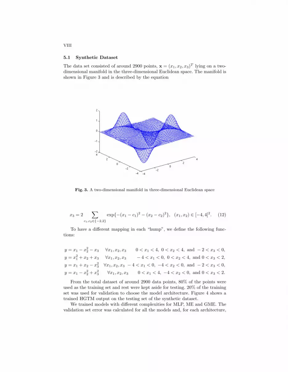
5.1 Synthetic Dataset

The data set consisted of around 2900 points, x = (x1, x2, x3)T lying on a two-dimensional manifold in the three-dimensional Euclidean space. The manifold isshown in Figure 3 and is described by the equation

Fig. 3. A two-dimensional manifold in three-dimensional Euclidean space

x3 = 2∑

c1,c2∈{−2,2}

exp{−(x1 − c1)2 − (x2 − c2)2}, (x1, x2) ∈ [−4, 4]2. (12)

To have a different mapping in each “hump”, we define the following func-tions:

y = x1 − x22 − x3 ∀x1, x2, x3 0 < x1 < 4, 0 < x2 < 4, and − 2 < x3 < 0,

y = x21 + x2 + x3 ∀x1, x2, x3 − 4 < x1 < 0, 0 < x2 < 4, and 0 < x3 < 2,

y = x1 + x2 − x23 ∀x1, x2, x3 − 4 < x1 < 0, −4 < x2 < 0, and − 2 < x3 < 0,

y = x1 − x22 + x2

3 ∀x1, x2, x3 0 < x1 < 4, −4 < x2 < 0, and 0 < x3 < 2.

From the total dataset of around 2900 data points, 80% of the points wereused as the training set and rest were kept aside for testing. 20% of the trainingset was used for validation to choose the model architecture. Figure 4 shows atrained HGTM output on the testing set of the synthetic dataset.

We trained models with different complexities for MLP, ME and GME. Thevalidation set error was calculated for all the models and, for each architecture,

IX

Fig. 4. HGTM visualisation output for the testing set of synthetic data

the model with the minimum validation set error was selected. The selectedmodel from a given class was then trained on the whole training set (includingthe validation set).

To analyse the properties of the input-space segmentation obtained fromME and GME, we measure its average entropy [7]. The average entropy wascalculated as below:

H = − 1M

M∑m=1

1N

N∑n=1

Pm(xn) log Pm(xn), (13)

where Pm(xn) log Pm(xn) is defined as 0 if Pm(xn) = 0. For ME, Pm(xn) is theoutput of the gating network for the mth expert, and input point xn, while forGME, Pm(xn) is the model responsibility, Rm,n. For the selected architectures,the average entropy values for ME and GME were obtained as 0.0621 and 0.0058respectively. These values reveal that the ME gives a comparatively soft segmen-tation with more overlaps, while the GME provides a harder segmentation whichseparates the input space in to distinct different regions with little overlap whichis also easier for the domain experts to interpret.

Table 1 presents the normalised mean squared error (NMSE) [8] we obtainedfor the training and the test sets. The 4th column in Table 1 displays the t-test significance value compared with the result of the GME. The t-test assesseswhether the means of two groups are statistically different from each other [9].The smaller the value, the more significant the difference between the means.Information about which model architecture was selected, using the validationset, is given in the last column. We note that the GME result is significantlybetter than the MLP and ME.

X

Table 1. Regression results for the synthetic dataset

Model Training NMSE Testing NMSE P-value Architecture

MLP 0.1009 0.0968 7.5816e-48 Nhid = 21

ME 0.0433 0.0466 0.0021 Nexperts = 11

GME 0.0234 0.0227 - Nexperts = 4

5.2 Chemoinformatics Data

The second experiment was carried out on a real life problem in the Chemoin-formatics domain where we need to predict the biological activity of chemicalcompounds, for a particular target, from 11 physicochemical properties of thecompounds. The dataset (of around 20700 chemical compounds selected ran-domly from around 1000000 compounds) was divided equally into training andtesting sets. 20% of the training set was kept aside for validation to choosethe model architecture. Figure 5 presents the HGTM visualisation output for asubset (random 600 compounds, 300 active and 300 inactive) of testing set.

Table 2. Regression results for biological activity prediction

Model Training NMSE Testing NMSE P-value Architecture

MLP 0.8439 0.8458 0.0129 Nhid = 25

ME 0.8370 0.8405 0.0200 Nexperts = 12

GME 0.8104 0.8214 - Nexperts = 7

The results are presented in Table 2. For the selected architectures, the av-erage entropy values for ME and GME were obtained as 0.1953 and 0.0298respectively which demonstrates better segmentation obtained by GME. TheGME result is better than the two models, though only at a level of 2%.

6 Discussion

Our approach of using visualisation output to develop guided local regressionmodels has given better results than the classical ME. That is in line with ourassumption that the segmentation obtained from principled visualisation algo-rithms, such as HGTM, can be sensibly used for the development of new localregression models.

The advantage of the approach is that the informed segmentation is obtainedwith the help of domain experts who have some understanding of the data in thisway, domain experts are more involved in the model development process. Thedisadvantage of GME is that, as a 2 stage process, it requires user interactionsand thus it takes comparatively more time to develop a new model.

XI

Fig. 5. HGTM output for the subset of the testing set of chemoinformatics data

XII

Overall, for the synthetic dataset, the local regression models gave betterresults than the global regression model. We believe that the principal localregression models, such as ME and GME, will perform well for high dimensionaldiverse datasets generally found in drug discovery and bioinformatics domains.

However, the experiments on chemical compounds gave NMSE of more than0.8 which is not satisfactory for practical use. The relatively high value of NMSEindicates that the models are close to predicting “in the mean” [8]. After dis-cussion with screening scientists, it was realised that the descriptors (11 physic-ochemical properties) used to predict the biological activities do not containenough information to make a robust prediction. Using structure information ofchemical compounds should help in improving regression models performancesince the pharmacophore1 of compounds plays an important role in making acompound active for a target [10].

Acknowledgements

DM is grateful to Pfizer Central Research for their financial support. We thankBruce S. Williams and Andreas Sewing for useful discussions on the results withthe Chemioinformatics data.

References

1. R. A. Jacobs, M. I. Jordan, S. J. Nowlan, G. E. Hinton, Adaptive mixture of localexperts, Neural Computation 3 (1991) 79–87.

2. P. Tino, I. T. Nabney, Constructing localized non-linear projection manifolds ina principled way: hierarchical generative topographic mapping., IEEE T. PatternAnalysis and Machine Intelligence 24 (2002) 639–656.

3. C. M. Bishop, M. Svensen, C. K. I. Williams, GTM: The generative topographicmapping, Neural Computation 10 (1998) 215–234.

4. F. Aurenhammer, Voronoi diagrams - survey of a fundamental geometric datastructure”, ACM Computing Surveys 3 (1991) 345–405.

5. C. M. Bishop, M. Svensen, C. K. I. Williams, Magnification factors for the GTMalgorithm, Proceedings IEE Fifth International Conference on Artificial NeuralNetworks (1997) 64–69.

6. P. Tino, I. T. Nabney, Y. Sun, Using directional curvatures to visualize foldingpatterns of the GTM projection manifolds, Artificial Neural Networks - ICANN(eds) G. Dorffner, H. Bischof and K. Hornik (2001) 421–428.

7. R. Ellis, Entropy, Large Deviations, and Statistical Mechanics, Springer-Verlag,New York, 1985.

8. C. M. Bishop, Neural Networks for Pattern Recognition, 1st Edition, Oxford Uni-versity Press, 1995.

9. N. Weiss, Elementary Statistics, 3rd Edition, Addison Wesley, 1996.10. A. C. Good, S. R. Krystek, J. S. Mason, High-throughput and virtual screening:

core lead discovery techologies move towards integration, Drug Discovery Today 5(2000) S61–S69.

1 A specific arrangement of chemical groups in a compound that are essential forrecognition by a target.