Embed Size (px)
Citation preview

This article was downloaded by: [ETH Zurich]On: 08 September 2014, At: 07:55Publisher: Taylor & FrancisInforma Ltd Registered in England and Wales Registered Number: 1072954 Registeredoffice: Mortimer House, 37-41 Mortimer Street, London W1T 3JH, UK
Combustion Theory and ModellingPublication details, including instructions for authors andsubscription information:http://www.tandfonline.com/loi/tctm20
Influence of turbulence–chemistryinteraction for n-heptane spraycombustion under diesel engineconditions with emphasis on sootformation and oxidationMichele Bollaa, Daniele Farracea, Yuri M. Wrighta, KonstantinosBoulouchosa & Epaminondas Mastorakosb
a Swiss Federal Institute of Technology, ETH Zurich, Switzerlandb University of Cambridge, UKPublished online: 07 Apr 2014.
To cite this article: Michele Bolla, Daniele Farrace, Yuri M. Wright, Konstantinos Boulouchos &Epaminondas Mastorakos (2014) Influence of turbulence–chemistry interaction for n-heptanespray combustion under diesel engine conditions with emphasis on soot formation and oxidation,Combustion Theory and Modelling, 18:2, 330-360, DOI: 10.1080/13647830.2014.898795
To link to this article: http://dx.doi.org/10.1080/13647830.2014.898795
PLEASE SCROLL DOWN FOR ARTICLE
Taylor & Francis makes every effort to ensure the accuracy of all the information (the“Content”) contained in the publications on our platform. However, Taylor & Francis,our agents, and our licensors make no representations or warranties whatsoever as tothe accuracy, completeness, or suitability for any purpose of the Content. Any opinionsand views expressed in this publication are the opinions and views of the authors,and are not the views of or endorsed by Taylor & Francis. The accuracy of the Contentshould not be relied upon and should be independently verified with primary sourcesof information. Taylor and Francis shall not be liable for any losses, actions, claims,proceedings, demands, costs, expenses, damages, and other liabilities whatsoeveror howsoever caused arising directly or indirectly in connection with, in relation to orarising out of the use of the Content.
This article may be used for research, teaching, and private study purposes. Anysubstantial or systematic reproduction, redistribution, reselling, loan, sub-licensing,systematic supply, or distribution in any form to anyone is expressly forbidden. Terms &

Conditions of access and use can be found at http://www.tandfonline.com/page/terms-and-conditions
Dow
nloa
ded
by [
ET
H Z
uric
h] a
t 07:
55 0
8 Se
ptem
ber
2014

Combustion Theory and Modelling, 2014
Vol. 18, No. 2, 330–360, http://dx.doi.org/10.1080/13647830.2014.898795
Influence of turbulence–chemistry interaction for n-heptane spraycombustion under diesel engine conditions with emphasis on soot
formation and oxidation
Michele Bollaa∗, Daniele Farracea, Yuri M. Wrighta, Konstantinos Boulouchosa andEpaminondas Mastorakosb
aSwiss Federal Institute of Technology, ETH Zurich, Switzerland; bUniversity of Cambridge, UK
(Received 13 November 2013; accepted 14 February 2014)
The influence of the turbulence–chemistry interaction (TCI) for n-heptane sprays underdiesel engine conditions has been investigated by means of computational fluid dy-namics (CFD) simulations. The conditional moment closure approach, which has beenpreviously validated thoroughly for such flows, and the homogeneous reactor (i.e. noturbulent combustion model) approach have been compared, in view of the recent resur-gence of the latter approaches for diesel engine CFD. Experimental data available froma constant-volume combustion chamber have been used for model validation purposesfor a broad range of conditions including variations in ambient oxygen (8–21% by vol.),ambient temperature (900 and 1000 K) and ambient density (14.8 and 30 kg/m3). Theresults from both numerical approaches have been compared to the experimental valuesof ignition delay (ID), flame lift-off length (LOL), and soot volume fraction distribu-tions. TCI was found to have a weak influence on ignition delay for the conditionssimulated, attributed to the low values of the scalar dissipation relative to the criticalvalue above which auto-ignition does not occur. In contrast, the flame LOL was consid-erably affected, in particular at low oxygen concentrations. Quasi-steady soot formationwas similar; however, pronounced differences in soot oxidation behaviour are reported.The differences were further emphasised for a case with short injection duration: in suchconditions, TCI was found to play a major role concerning the soot oxidation behaviourbecause of the importance of soot-oxidiser structure in mixture fraction space. Neglect-ing TCI leads to a strong over-estimation of soot oxidation after the end of injection.The results suggest that for some engines, and for some phenomena, the neglect ofturbulent fluctuations may lead to predictions of acceptable engineering accuracy, butthat a proper turbulent combustion model is needed for more reliable results.
Keywords: conditional moment Closure; soot modelling; turbulence-chemistryinteraction; diesel engines, spray combustion
1 Introduction
Numerical simulations are becoming a valuable tool for assistance in product development.Nowadays, direct numerical simulation (DNS) is a powerful tool for the understandingof processes at the molecular level; however, for engineering relevant applications (e.g.diesel engines and gas turbines) with very high Reynolds numbers and fuels with com-plex oxidation kinetics, the costs of DNS are still prohibitive. In the past four decadesthe understanding of turbulent combustion has seen a formidable improvement from anexperimental as well as a modelling perspective. Significant effort has been allocated to
∗Corresponding author. Email: [email protected]
C© 2014 Taylor & Francis
Dow
nloa
ded
by [
ET
H Z
uric
h] a
t 07:
55 0
8 Se
ptem
ber
2014
Combustion Theory and Modelling 331
the modelling of turbulence–chemistry interaction (TCI), in particular due to the stronglynonlinear behaviour of the chemical source term. The importance of TCI and the conse-quent need for a combustion model has been clearly demonstrated for many fundamentalconfigurations such as laboratory flames, especially in view of predictions of auto-ignitionand extinction processes as well as emissions [1]. Therefore, virtually every research effortrelated to turbulent flames proposed in the literature employs a TCI closure. Most commonmodels are the probability density function (PDF) [2, 3], flamelet/progress variable (FPV)[4] and conditional moment closure (CMC) [5, 6], amongst others. Soot formation has alsobeen successfully modelled using the aforementioned approaches (PDF [2], FPV [7], CMC[8, 9]).
For the auto-ignition process in diesel engines, the conventional modelling approachin the past has been to solve transport equations for the ensemble-averaged reacting scalarmass fractions using chemical source terms with semi-empirical Arrhenius expressions[10], but completely neglecting turbulent fluctuations. One justification for this widelyadopted ‘shell model’ was that the chemistry of auto-ignition is slow relative to the turbulenttimescale. An additional pragmatic reason was that, at that time, no comprehensive turbulentreacting flow models that could be used for problems for a wide range of Damkohlernumbers were available. In this relatively dated, conventional approach, after auto-ignitionthe model switched to a turbulent combustion model for the non-premixed part of the dieselcombustion process (e.g. Magnussen’s eddy dissipation) [11, 12]. With the development ofthe flamelet model in the 1990s, more advanced turbulent combustion theories started toappear in the field of diesel engine computational fluid dynamics (CFD) [13–15], and morerecently, all advanced combustion models are being used: CMC [16–21], PDF [22–25],partially stirred reactor [26], generalised flame surface density model [27], FPV models[28] and the flamelet generated manifold method [29].
Together with this trend, chemistries with increasing detail are being proposed in orderto capture accurately the auto-ignition times of various fuels [30], especially in view of‘new’ fuels including oxygenated or bio-derived components or alternative combustionmodes such as low-temperature combustion or homogeneous charge compression ignition.This increases the cost of the calculation; thus, some authors have reverted back to theold practice of neglecting turbulent fluctuations but still using chemistry to any level ofcomplexity. Therefore, the CFD solves transport equations for the mean mass fractionsof n−1 scalars, where n is the number of species participating in the chemical scheme,with the mean chemical source term evaluated at these mean mass fractions and meantemperature. This makes sense only if the fluctuations are negligible, or only if somehowthey matter little for the prediction of some quantities of interest. In principle, turbulencetheory dictates that if the mean scalar mass fraction has an inhomogeneity in space (andtherefore there is a need to solve a transport equation for it), fluctuations are generated.It is clear therefore that neglecting turbulent fluctuations at the outset is fundamentallyhighly questionable. Despite this, some reasonable predictions are claimed when using thisapproach [31], which has stimulated various studies seeking to clarify why this might bethe case at certain engine relevant conditions. These investigations are directly linked tothe emergence of high-fidelity experimental data from the last decade which has proveninstrumental for detailed validation of in-cylinder processes. In particular in the contextof the Engine Combustion Network (ECN), a large database of experimental data fromdifferent optically accessible high-pressure vessels has arisen [32] and has encouragednumerous recent modelling activities for well-defined target conditions. Particular attentionhas been devoted to the reactive n-heptane test cases from this database, as can be seenfrom the comprehensive review of simulation activities using a variety of established models
Dow
nloa
ded
by [
ET
H Z
uric
h] a
t 07:
55 0
8 Se
ptem
ber
2014

332 Michele Bolla et al.
presented in [23]. More recently, reactive n-dodecane sprays have also been the focus ofattention as summarised in [24]. Both former studies [23, 24] and also [22] employ acomposition PDF model and highlight in detail the importance of TCI for a wide rangeof conditions by comparing the results with calculations neglecting turbulent fluctuations.Further studies reporting such comparisons using flamelet models have been reported in[33–35].
As shown in [23], the use of a composition PDF method compared to a well-mixedassumption was shown generally to improve the predictions of ignition delay and LOL.Findings put forward in [24] further reveal that, especially at high levels of dilution, theneglect of TCI can lead to erroneous predictions and the flame brush structure predictedwhen neglecting turbulent fluctuations is considered implausible.
Further to the investigations reported in [22–24] using the composition PDF approach,this study employs a well-proven CMC combustion model [16–21, 36] in conjunctionwith an embedded soot model [37] to study the impact of neglecting TCI with particularemphasis on emissions. The present investigation additionally seeks to elucidate the reasonsbehind the apparent success of neglecting TCI by examining the predicted ignition delays,LOLs and soot distributions for a variety of diesel engine relevant conditions. Furthermore,understanding is provided with respect to the limitations of the approach, particularlyconcerning the prediction of soot oxidation.
The remainder of the paper is structured as follows. First, the numerical methodology ispresented including the combustion and soot modelling approaches. In a second step, resultsare compared in terms of ignition delay, flame LOL and quasi-steady soot distributions.Subsequently, differences in soot evolution are analysed. In the last section, the soot temporalevolution is considered for short injection durations in order to validate the soot oxidationrate.
2 Numerical methodology
In this section, the numerical methodology is presented. It consists of the CFD flow fieldsolver followed by the CMC formulation for the combustion as well as the soot model. Themethodology follows largely what has already been presented in [16] and CMC referencestherein; the main features are, nevertheless, repeated here for completeness. The soot modelhas been complemented to account for differential diffusion, for which the governingequations are also given below.
2.1 Flow field solver
The flow field has been treated with the commercial CFD code Star-CD [38], a fully-compressible finite-volume solver. As a symmetric spray arrangement is considered, aquasi-2D grid with one degree angle was used with a homogeneous resolution of 0.5 ×0.5 mm2 size in the first 15 mm radially along the entire axial domain, while in the outerpart a constant cell size of 1 × 1 mm2was employed. This resolution was found to beappropriate in previous simulations [16] for the same spray setup and is in line with ECNrecommendations [32]. The width of the domain has been adjusted in order to match thechamber volume. The Reynolds Averaged Navier–Stokes (RANS) equations are solvedand the turbulent stresses are closed with the k–ε RNG model with Star-CD default modelcoefficients and the corresponding ‘standard’ wall functions [38]. A PISO based solver isemployed with a constant time step of 1 × 10⁻⁶ seconds.
Dow
nloa
ded
by [
ET
H Z
uric
h] a
t 07:
55 0
8 Se
ptem
ber
2014

Combustion Theory and Modelling 333
The liquid phase of the spray is treated in a Lagrangian way consisting of the ‘blob’model for primary and the Reitz–Diwakar model for secondary breakup [39]. Droplet–droplet collisions are modelled according to O’Rourke [40] and turbulent dispersion isdescribed with a stochastic formulation. Droplet evaporation and heat transfer is computedwith the Ranz–Marshall approach and drag forces are considered to be dynamic [38].The thermo-physical properties of n-heptane droplets (density, viscosity, latent heat, heatcapacity, surface tension and saturation pressure) are computed as a function of temperature.The measured injection rate is imposed for the simulation.
For the well-mixed method (i.e. where no turbulent combustion model is used), alsodenoted as ‘direct integration’ (DI) method to be consistent with some of the relatedliterature, a transport equation is solved at the CFD resolution for each species and enthalpy,with mean chemical source terms calculated based on the mean temperature, mean speciesmass fractions, and the respective cell pressure and hence neglecting turbulent fluctuations.Note that the CFD resolution (0.5 × 0.5 mm2) is the same as for CMC.
For the CMC approach, only the ‘chemico-thermal’ enthalpy equation is solved in CFD.No transport equation for chemical species is needed, as mean species mass fractions areobtained by convolution of the conditional species mass fraction with the presumed mixturefraction (MF) PDF evaluated at every CFD cell. Here, the β-PDF has been assumed, whichis determined by solving the transport equations for their first two moments, i.e. the mean(Equation 1) and the variance (Equation 2) of the MF as follows:
∂ρξ
∂t+ ∇
[ρuj ξ −
(ρDξ + μt
Scξ
)∇ ξ
]= Sd , (1)
∂ρξ ′′2
∂t+ ∇
[ρuj ξ ′′2 −
(ρDξ ′′2 + μt
Scξ ′′2
)∇ ξ ′′2
]= 2μt
Scξ ′′2
(∇ ξ)2 − ρχ , (2)
where the mean MF source corresponds to fuel evaporation. In the literature, various modelclosures for the influence of droplet evaporation on mixture fraction variance (MFV) havebeen proposed, e.g. [41]. In this study, this effect has been neglected since the influence ofdroplets has been previously investigated in [17] for the same experimental configurationand only marginal differences in ID and flame LOL were reported. This may be expectedsince there is a clear spatial separation between the region of evaporation and the flame andsoot region, in particular for dilute cases. Neglecting these terms here is also consistentwith their neglect in the DI approach, since a comparison is one of the targets of this paper.
The mean scalar dissipation rate (SDR) has been modelled as
χ = cχ
ε
kξ ′′2, (3)
where cχ is a model constant set to 2.0 as was the case in previous CMC spray studies, e.g.[20].
2.2 CMC formulation
In CMC, transport equations are solved for conditionally averaged reactive scalars. For adetailed derivation of the CMC governing equations, the reader is referred to [42]; here,only a brief presentation of the equations follows. As shown in [42], transport equations for
Dow
nloa
ded
by [
ET
H Z
uric
h] a
t 07:
55 0
8 Se
ptem
ber
2014

334 Michele Bolla et al.
the conditional species mass fractions (Equation 4) and conditional temperature (Equation5) can be derived which, in a RANS context, read as
∂Qα
∂t+ 〈ui | η〉 ∂Qα
∂xi
+ 1
ρP (η)
∂
∂xi
[⟨ρu′′
i Y′′α
∣∣ η⟩P (η)
] − 〈N | η〉 ∂2Qα
∂η2= 〈wα | η〉 ,
(4)
∂QT
∂t+ 〈ui | η〉 ∂QT
∂xi
+ 1
ρP (η)
∂
∂xi
[⟨u′′
i T′′ ∣∣ η
⟩ρP (η)
] − 〈N | η〉 ∂2QT
∂η2
− 〈N | η〉[
1
〈cP | η〉
(∂ 〈cP | η〉
∂η+
N∑α=1
⟨cP,α | η ⟩ ∂Qα
∂η
)]∂QT
∂η
= 1
〈cP | η〉⟨
1
ρ
∂P
∂t
∣∣∣∣ η
⟩+ 〈wT | η〉
〈ρ | η〉 〈cP | η〉 + 〈wWALL | η 〉〈ρ | η 〉 〈cP | η 〉
− 〈 | η〉[
hfg
〈cP | η〉 + QT + (1 − η)∂QT
∂η
]− 1
ρP (η)
∂
∂η
[(1 − η) ρP (η)
⟨T ′′′′ ∣∣ η
⟩], (5)
where 〈·|ξ=η〉 denotes ensemble averaging of the quantity on the left side of the verticalbar, subject to the sample space variable value fulfilling the condition on the right side of thevertical bar. The CMC governing equations are four dimensional (three in space plus onefor the MF) and include terms accounting for transport in physical space due to convectionand turbulent fluxes – terms 2 and 3 on the left-hand side (LHS) of Equations (6) and (7)– whereas term 4 corresponds to transport in MF space due to molecular mixing, hereapproximated by the amplitude mapping closure (AMC) model. Conditional velocity isclosed with a linear approach and a gradient flux assumption is applied for turbulent fluxes.The effects of evaporating droplets, represented by the last two terms on the right-hand side(RHS) of Equation (5), are implemented as put forward in [17].
The conditional chemical source terms due to reaction are closed at first order, as thisapproach has seen highly successful application to a number of spray combustion problemsin generic test rigs [16, 17, 20, 43, 44]. In this study, the reduced n-heptane chemistryproposed by [45] has been employed, which has shown very good predictive capabilities forauto-igniting sprays for a broad range of conditions [16, 43, 44]. The mechanism consistsof 22 solved species and 18 reactions.
As discussed in [42], the conditional quantities exhibit far weaker spatial dependencecompared to their unconditional values. As a consequence, a much lower resolution canbe used for the CMC grid than is needed for the CFD grid. Motivated by the good resultsreported in [16], here, the same CMC resolution of 2 by 1 mm in axial and radial resolutionis employed, resulting in 54 × 20 CMC nodes. Conserved scalar space is discretisedin 101 points clustered around stoichiometry. Further details concerning the numericaldiscretisation procedure and time integration of the system are not give here, but can befound in [17, 19, 20], for example.
Dow
nloa
ded
by [
ET
H Z
uric
h] a
t 07:
55 0
8 Se
ptem
ber
2014
Combustion Theory and Modelling 335
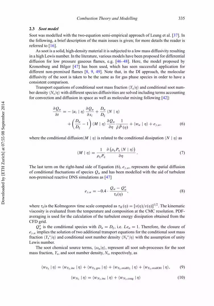
2.3 Soot model
Soot was modelled with the two-equation semi-empirical approach of Leung et al. [37]. Inthe following, a brief description of the main issues is given; for more details the reader isreferred to [16].
As soot is a solid, high-density material it is subjected to a low mass diffusivity resultingin a high Lewis number. In the literature, various models have been proposed for differentialdiffusion for low pressure gaseous flames, e.g. [46–48]. Here, the model proposed byKronenburg and Bilger [47] has been used, which has seen successful application fordifferent non-premixed flames [8, 9, 49]. Note that, in the DI approach, the moleculardiffusivity of the soot is taken to be the same as for gas phase species in order to have aconsistent comparison.
Transport equations of conditional soot mass fraction 〈Ys|η〉 and conditional soot num-ber density 〈Ns|η〉 with different species diffusivities are solved including terms accountingfor convection and diffusion in space as well as molecular mixing following [42]:
∂Qα
∂t= −〈ui | η〉 ∂Qα
∂xi
+ Dα
Dξ
〈N | η〉
+(
Dα
Dξ
− 1
)〈M | η〉 ∂Qα
∂η
1
ρP (η)+ 〈wα | η〉 + ey,α, (6)
where the conditional diffusion〈M | η〉 is related to the conditional dissipation 〈N | η〉 as
〈M | η〉 = 1
ρηPη
∂(ρηPη 〈N | η〉)
∂η. (7)
The last term on the right-hand side of Equation (6), ey,α , represents the spatial diffusionof conditional fluctuations of species Qα and has been modelled with the aid of turbulentnon-premixed reactive DNS simulations as [47]
ey,α = −0.4 · Qα − Q∗α
τk(η), (8)
where τkis the Kolmogorov time scale computed as τK (η) = [ν(η)/ε(η)]1/2. The kinematicviscosity is evaluated from the temperature and composition at the CMC resolution. PDF-averaging is used for the calculation of the turbulent energy dissipation obtained from theCFD grid.
Q∗α is the conditional species with Dα = Dξ , i.e. Leα = 1. Therefore, the closure of
ey,α implies the solution of two additional transport equations for the conditional soot massfraction 〈Ys
∗|η〉 and conditional soot number density 〈Ns∗|η〉 with the assumption of unity
Lewis number.The soot chemical source terms, 〈ωα |η〉, represent all soot sub-processes for the soot
mass fraction, Ys, and soot number density, Ns, respectively, as
〈wYS | η〉 = 〈wYS,inc | η〉 + 〈wYS,gro | η〉 + 〈wYS,oxidO2 | η〉 + 〈wYS,oxidOH | η〉, (9)
〈wNS| η〉 = 〈wNS,inc | η〉 + 〈wNS,coag | η〉 (10)
Dow
nloa
ded
by [
ET
H Z
uric
h] a
t 07:
55 0
8 Se
ptem
ber
2014

336 Michele Bolla et al.
Table 1. Soot chemistry mechanism [37].
Reaction Reaction rate
(I) C2H2Rn→ 2C(S) + H2 Rn = kn[C2H2]
(II) C2H2 + nC(S)Rg→ (n + 2) C(S) + H2 Rg = kg[C2H2]
(III) C(S) + 0.5O2
RO2→ CO RO2 = kO2 [O2]
(IV) C(S) + OHROH→ CO + H ROH = kOH[OH]
where terms accounting for simultaneous soot inception, surface growth, oxidation by O2
and OH, and particle coagulation are considered. The individual chemical reactions andthe corresponding rates are summarised in Table 1 and Table 2, respectively. Note that,for DI, the soot transport equations are solved with the same soot mechanism constants,however at the CFD resolution and using mean quantities as was the case for the speciesmass fractions. Acetylene has been considered for both soot inception and soot surfacegrowth. Here, the focus is on TCI and this simplifying assumption has been adopted basedon the good agreement of soot distributions and absolute values demonstrated in a previousinvestigation for sprays in the current constant-volume spray test rig [16]. Nevertheless,future studies should assess the influence on the predictions depending on the choice of thesoot precursor in detail. Soot particle coagulation is modelled following Leung et al. [37 ].
Soot radiation has been considered with an optically thin assumption, where radiationis considered for major gaseous species (CO2, CO, H2O and CH4) according to [50] andsoot with absorptivity properties reported in [51]. A more complex radiation model, e.g.the discrete ordinate method [52], has not been attempted here.
2.4 Test cases
Experimental data available from the constant volume chamber at Sandia National Labo-ratories [32] has been used for model validation. The optically-accessible cell has a cubicshape with a side length of 108 mm and the injector is mounted in the middle of one surface.The measurement of ignition delay is based on the pressure with a correction for the speedof sound. LOL is determined by means of OH∗chemiluminescence, and soot volume frac-tion under quasi-steady conditions is measured with planar laser induced incandescence(PLII) with a calibration against laser extinction measurements. For a detailed descrip-tion of the experimental setup and the measurement techniques, the reader is referred to[53, 54] and references therein. A broad range of experimental conditions have been mea-sured, including variations in fuel, fuel pressure, nozzle orifice diameter, temperature,density, and oxygen content of the oxidiser.
Table 2. Soot formation and oxidation reaction rate constants in Arrhenius form, kj = A · T b ·exp
(−Ta
/T
) · SCSoot . Units are in kg, kmol, m, s, K. [From Leung et al. [37].
kj A b Ta c Reference
(I) Inception kn 1.0e4 0 21100 0 [37](II) Surface growth kg 3.0e3 0 12100 0.5 [37](III) Oxidation by O2 kO2 1.0e4 0.5 19800 1 [37](IV) Oxidation by OH kOH 0.36 0.5 0 1 [8]
Dow
nloa
ded
by [
ET
H Z
uric
h] a
t 07:
55 0
8 Se
ptem
ber
2014
Combustion Theory and Modelling 337
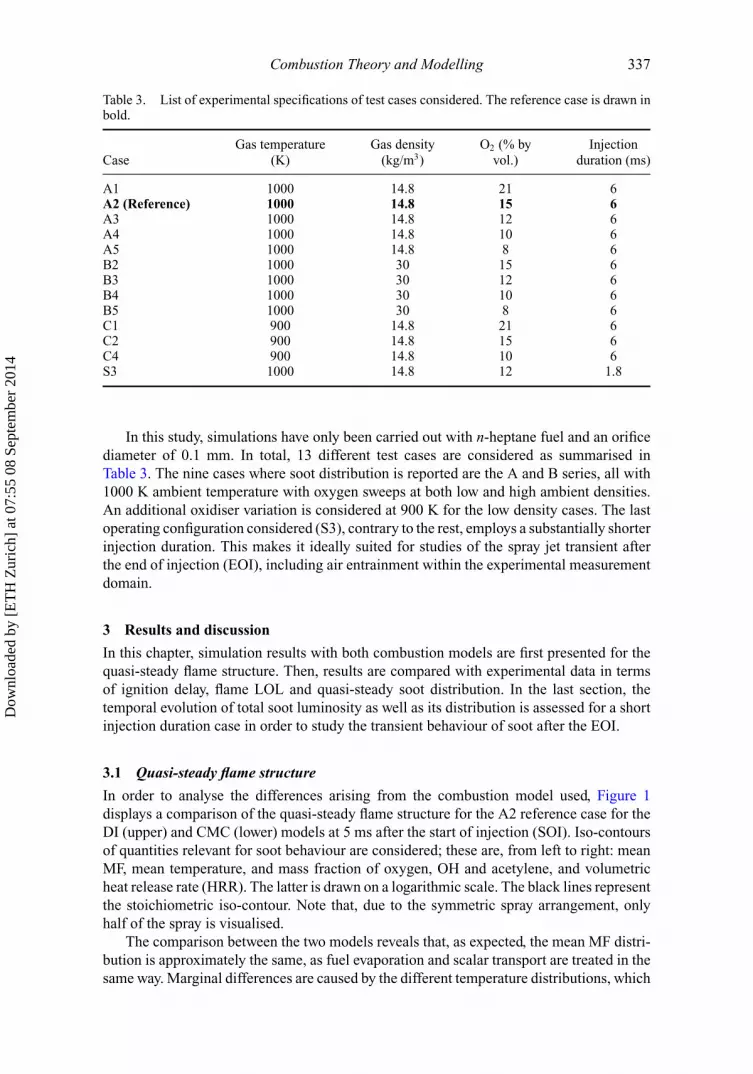
Table 3. List of experimental specifications of test cases considered. The reference case is drawn inbold.
Gas temperature Gas density O2 (% by InjectionCase (K) (kg/m3) vol.) duration (ms)
A1 1000 14.8 21 6A2 (Reference) 1000 14.8 15 6A3 1000 14.8 12 6A4 1000 14.8 10 6A5 1000 14.8 8 6B2 1000 30 15 6B3 1000 30 12 6B4 1000 30 10 6B5 1000 30 8 6C1 900 14.8 21 6C2 900 14.8 15 6C4 900 14.8 10 6S3 1000 14.8 12 1.8
In this study, simulations have only been carried out with n-heptane fuel and an orificediameter of 0.1 mm. In total, 13 different test cases are considered as summarised inTable 3. The nine cases where soot distribution is reported are the A and B series, all with1000 K ambient temperature with oxygen sweeps at both low and high ambient densities.An additional oxidiser variation is considered at 900 K for the low density cases. The lastoperating configuration considered (S3), contrary to the rest, employs a substantially shorterinjection duration. This makes it ideally suited for studies of the spray jet transient afterthe end of injection (EOI), including air entrainment within the experimental measurementdomain.
3 Results and discussion
In this chapter, simulation results with both combustion models are first presented for thequasi-steady flame structure. Then, results are compared with experimental data in termsof ignition delay, flame LOL and quasi-steady soot distribution. In the last section, thetemporal evolution of total soot luminosity as well as its distribution is assessed for a shortinjection duration case in order to study the transient behaviour of soot after the EOI.
3.1 Quasi-steady flame structure
In order to analyse the differences arising from the combustion model used, Figure 1displays a comparison of the quasi-steady flame structure for the A2 reference case for theDI (upper) and CMC (lower) models at 5 ms after the start of injection (SOI). Iso-contoursof quantities relevant for soot behaviour are considered; these are, from left to right: meanMF, mean temperature, and mass fraction of oxygen, OH and acetylene, and volumetricheat release rate (HRR). The latter is drawn on a logarithmic scale. The black lines representthe stoichiometric iso-contour. Note that, due to the symmetric spray arrangement, onlyhalf of the spray is visualised.
The comparison between the two models reveals that, as expected, the mean MF distri-bution is approximately the same, as fuel evaporation and scalar transport are treated in thesame way. Marginal differences are caused by the different temperature distributions, which
Dow
nloa
ded
by [
ET
H Z
uric
h] a
t 07:
55 0
8 Se
ptem
ber
2014

338 Michele Bolla et al.
Figure 1. Spatial distribution of relevant quantities for flame characterisation at 5 ms after SOI forthe reference case A2 computed with (a) DI and (b) CMC. From left to right: mean MF, temperature,mass fractions of acetylene, oxygen, OH and CH2O, respectively. The black line denotes the locationof the stoichiometric MF ξST.
Dow
nloa
ded
by [
ET
H Z
uric
h] a
t 07:
55 0
8 Se
ptem
ber
2014

Combustion Theory and Modelling 339
influence the fuel evaporation. The main difference between the two computed flames liesin the spatial distribution of oxygen. With DI the oxygen is completely consumed at thestoichiometric iso-line and no oxygen is left in the fuel rich region. On the other hand,the CMC method predicts a certain stratification also in the rich region. This broadeningis expected in turbulent combustion and is due to the description of the MF through aPDF. However, oxygen is completely consumed in MF space for some MF. The DI caseresults in a much thinner layer of OH along stoichiometry as well as a thinner layer withhigh chemical activity as revealed by the HRR distribution. The peak OH mass fractionpredicted by DI is approximately twice as high as the corresponding CMC value, but in asmaller volume; as a consequence, the resulting field totals are of roughly the same order.
As expected, for both models the highest HRR is found at the LOL; downstream alongthe stoichiometric iso-contour, a diffusion flame is established with one or two ordersof magnitude lower HRR. There is also a rich premixed branch in the inner part of thespray starting from the anchoring point, consistent with the conceptual model proposed byIdicheria and Pickett [55]. For both models, the HRR exhibits the same spatial extent as forthe OH species.
The thin OH layer obtained when using DI is consistent with former DI studies for adiesel spray, e.g. [23, 56]. Comparison of OH profiles using different combustion modelswas also the focus of the ECN2 workshop and the same trends were reported [32]. For theexperiment considered in this study, there is no OH-PLIF (planar laser induced fluorescence)measurement available. However, under similar conditions, LIF measurements have beenperformed and instantaneous OH profiles were found to be considerably thin (less than1 mm), e.g. [54, 57, 58]. At this point it should be recalled however that the RANSsolution is representative for an ensemble average over many injection events. Images ofOH∗ chemiluminescence show a considerable fluttering of the flame and soot region [32].Applying ensemble averaging over many injection events, a thicker averaged OH profileis hence to be expected, as also discussed in [24], where the thin flame predicted by DI isconsidered implausible compared to the flame brush structure predicted by the compositionPDF employed.
As a consequence, the peak mean temperature exhibits higher values for DI. The lowerpeak mean temperature of CMC is, again, caused by the PDF description of the localcomposition. In this specific case the difference is approximately 100 K.
As acetylene is the unique species responsible for soot formation in the model employedhere, it is important to compare its distribution for later soot predictions. For the two modelsstudied, a similar structure and the same concentration values are found. The spread of thesoot precursor is, however, larger for the CMC for the same reason as that for the MF PDFdiscussed above, hence there is some acetylene escaping in the mean fuel lean region.
The flame lift-off position is clearly visible, due to the strong axial gradient of meantemperature and OH mass fraction. For the reference case A2, DI estimates a slightly higherLOL, as will be discussed next.
3.2 Ignition delay and lift-off length
ID and lift-off length were both defined according to the ECN recommendations [32]: IDwas defined as the time after SOI when the maximal rate of change of peak temperaturewithin the domain occurs, while the flame LOL has been determined as the minimal axialdistance from the injector tip where a threshold value of 2% of the peak OH mass fractionis present. Figure 2 compares ID time (left) and flame LOL (right) for the two combustionmodels against experimental data for ambient oxygen variations at three different ambient
Dow
nloa
ded
by [
ET
H Z
uric
h] a
t 07:
55 0
8 Se
ptem
ber
2014
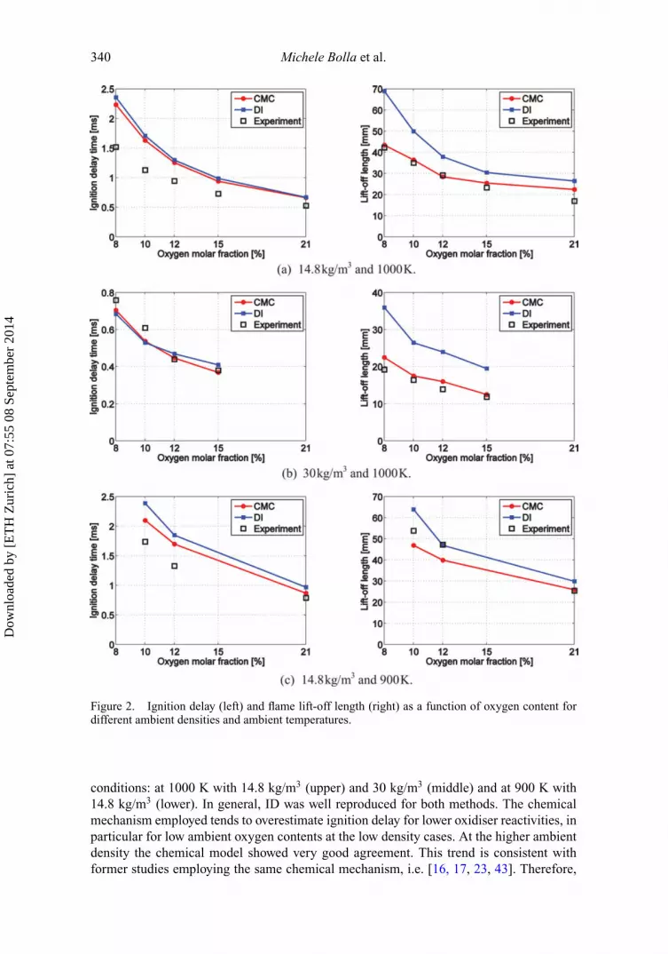
340 Michele Bolla et al.
Figure 2. Ignition delay (left) and flame lift-off length (right) as a function of oxygen content fordifferent ambient densities and ambient temperatures.
conditions: at 1000 K with 14.8 kg/m3 (upper) and 30 kg/m3 (middle) and at 900 K with14.8 kg/m3 (lower). In general, ID was well reproduced for both methods. The chemicalmechanism employed tends to overestimate ignition delay for lower oxidiser reactivities, inparticular for low ambient oxygen contents at the low density cases. At the higher ambientdensity the chemical model showed very good agreement. This trend is consistent withformer studies employing the same chemical mechanism, i.e. [16, 17, 23, 43]. Therefore,
Dow
nloa
ded
by [
ET
H Z
uric
h] a
t 07:
55 0
8 Se
ptem
ber
2014

Combustion Theory and Modelling 341
the influence of TCI on auto-ignition is found to be comparatively small throughout theentire range of conditions considered here.
As far as flame LOL is concerned, both models capture the correct trend with anincrease in LOL by decreasing oxygen content. Here, the influence of the combustionmodel is seen to be more important. DI predicts a larger LOL for all cases, in particularat the lower ambient density and low oxygen volume fractions, where LOL is considerablyoverestimated.
The above observations are in line with the results reported in [22] showing the com-parison of DI with the transported PDF method for the same n-heptane spray consideredhere where it was found that neglecting turbulent fluctuations has a minor influence on ID,whereas considerable increase in LOL has been observed. In the following, reasons for theobserved behaviours in ID and LOL are further analysed. There are a few main differencesbetween the models. First, the DI considers the computational cell as well-mixed, whereasCMC assumes the MF distribution within the computational cell to be a β-function. Differ-ences in average HRR decrease by diminishing MFV. Second, CMC includes the SDR asan important parameter that represents molecular mixing, a phenomenon which is missingfrom the DI formulation. At high levels of SDR, auto-ignition is delayed or even completelyinhibited [1]. For the limit case of zero variance and zero SDR, the CMC becomes identicalwith the well-mixed assumption that implies a delta function for the species PDFs at themean values and no small-scale mixing effects on the reaction rate.
Discussion of ignition delayAuto-ignition of non-premixed flames is a complex process, a review of which can be foundin [1]. Auto-ignition is known to occur at a characteristic MF, the so-called most reactiveMF [59], which for higher hydrocarbons such as n-heptane under diesel engine conditionshas been seen to be rich [19, 20]. Recently, DNS results of auto-ignition of n-heptanedroplets at high temperature and pressure confirmed that the concept of most reactive MFis still valid for evaporating auto-igniting droplets [60].
Here, as a preliminary step to study the influence of SDR on auto-ignition under dieselengine conditions, transient flamelet calculations according to [13] have been carried outwith different conditional SDR applying the AMC model [61] for all five ambient dilutionsat the higher temperature (1000 K) and the lower ambient density (14.8 kg/m3) conditions.Results are shown in Figure 3 in terms of ID versus SDR at the most reactive MF. The mostreactive MF has been determined for every oxidiser dilution assuming zero SDR followingcommon practice, i.e. [1, 19]. The most reactive MF was found to remain in a confinedequivalence ratio range of 2–2.5, as illustrated in Figure 3 (right), while the stoichiometricMF obeyed a linear decrease for increasing dilution. As expected, low values of SDR haveminor influence on ignition delay, as can be seen for all states of dilution. The respective,relatively constant delay times are however considerably higher for the diluted cases dueto the substantial reduction in reactivity of the oxidiser. For higher SDR, auto-ignition isincreasingly inhibited and the critical SDR values, at which ignition can no longer occur,also decrease with oxidiser dilution as the mixture becomes less reactive. For the referencecase with 15% O2, values of SDR at the most reactive MF up to 15 s−1 have a marginalinfluence on ID and this value is of relevance for later discussion.
The reference case A2 is considered next to study the temporal history of temperature,SDR, and two low-temperature pre-ignition species CH2O and H2O2. The flow field prior toauto-ignition, i.e. at 0.7 ms after SOI (the computed ID is approx. 0.9 ms for both models) isdisplayed in Figure 4. From left to right: mean MF, mean temperature, mean SDR, and massfraction of CH2O for both CMC and DI. Note that the MF and temperature distributions
Dow
nloa
ded
by [
ET
H Z
uric
h] a
t 07:
55 0
8 Se
ptem
ber
2014

342 Michele Bolla et al.
Figure 3. Left: stoichiometric and most reactive MF at different ambient dilutions. Right: flameletcalculation results for ignition delay at different values of SDR at 1000 K and 14.8 kg/m3 ambienttemperature and density, respectively.
Figure 4. Reference case A2, 0.7 ms after SOI. Mean MF, temperature and mean scalar dissipationrate are for CMC. Points represent the position of the auto-igniting fluid particle at different timesafter SOI in milliseconds.
are illustrated for the CMC solution since results with DI are very similar prior to ignitionas discussed above and have therefore been omitted for brevity. The mean SDR exhibitshigh values at locations where considerable spatial gradients of the MF are present (cf.the production term on the RHS of Equation 2) and very low SDR is increasingly foundtowards the tip of the spray. Both the concentration and spatial extent of CH2O were foundto be almost equivalent between the models. The highest auto-ignition activity is closeto the spray tip where higher temperature in conjunction with low SDR is beneficial forauto-ignition. As a consequence, the predicted location of the ignition spot was found to bevirtually identical for both models with a difference of 1 mm.
The first auto-igniting fluid particle has been tracked (following the mean velocity vectorand neglecting turbulent dispersion) in order to describe the difference in temporal history
Dow
nloa
ded
by [
ET
H Z
uric
h] a
t 07:
55 0
8 Se
ptem
ber
2014

Combustion Theory and Modelling 343
Figure 5. Temporal evolution of temperature, CH2O and H2O2 and conditional scalar dissipationrate at most reactive MF along first auto-igniting fluid particle for the reference case A2 for DI (dashedlines) and CMC (solid lines).
of chemical activity. The black points in Figure 4 corresponds to the trajectory of the auto-igniting fluid particle at the given time instants denoted by the numbers in milliseconds.The time instant of 0.7 ms, for which the spatial distributions are shown, corresponds to theCH2O peak where ignition activity is the highest. The temporal evolution of temperature,conditional SDR at the most reactive MF, and auto-ignition species CH2O and H2O2 alongthe trajectory are drawn in Figure 5. For the early time instants where the fluid particle isstill located in the core of the spray, the gas temperature is below 800 K due to evaporationand air/fuel mixing. The gradual increase in temperature until high-temperature ignitionis mostly due to the mixture’s becoming leaner downstream rather than due to the HRR.Of primary importance is the evolution of SDR, showing high values in the first phaseup to 0.4 ms; at later instants very low values are present, well below the critical value.Therefore, the delaying effect of turbulent straining on auto-ignition is limited to thevery early regions of the spray and the overall ignition delay time is hardly affected, asemphasised in Figure 3. The evolution of CH2O and H2O2 exhibited similar behaviour witha rapid increase in concentration during low-temperature pre-ignition activity and a periodwith nearly constant concentration and rapid consumption during the high-temperatureauto-ignition. H2O2 is found to be consumed slightly earlier and the two models showedvery similar behaviour. Generally, for DI, higher rates of change of species mass fractionand temperature were observed. Low-temperature species CH2O and H2O2 were formedslightly later with DI, which is probably due to the low mean temperature present there thataffects chemical activities. The difference in peak temperature after auto-ignition is due tothe thinner flame and complete consumption of oxygen as discussed earlier in the contextof Figure 1.
Along the same fluid particle, conditional temperature and CH2O are illustrated inFigure 6. From the temperature evolution, it is clearly visible that the most reactive MF is ataround 0.12–0.14, in agreement with the values determined by the stand-alone calculationfor this reference condition (cf. Figure 3). A subsequent rapid transition of the peak condi-tional temperature towards stoichiometric conditions can be clearly observed. On the otherhand, CH2O is increasingly formed in the fuel rich region prior to auto-ignition and starts tobe rapidly consumed at the onset of ignition at 0.85 ms in the presence of high-temperaturereactions as is clearly visible from the ‘dent’ at the most reactive MF and continuing towards
Dow
nloa
ded
by [
ET
H Z
uric
h] a
t 07:
55 0
8 Se
ptem
ber
2014

344 Michele Bolla et al.
Figure 6. Evolution of conditional temperature (left) and CH2O mass fraction (right) along firstauto-igniting fluid particle for the reference case A2. Vertical dashed lines denote stoichiometric MFξST.
leaner conditions. The same dynamic is encountered for H2O2 and therefore not presentedhere.
Overall, both models showed comparable results and confirm that auto-ignition underdiesel engine conditions occurs prevalently at low values of SDR, much lower than thecritical value, where TCI plays a minor role because the molecular mixing delaying effectsare small. Although not shown here, the same argumentation also applies to the otheroperating conditions considered and explains why good ignition delay predictions can beachieved with DI despite the neglect of the turbulent fluctuations. It is important to note thatalthough dilution substantially decreases the critical SDR (as shown in Figure 3, left), theeffective SDR a particle experiences decreases as well since the ignition location is shiftedfurther downstream as a consequence of the lower reactivity, as has also been observedexperimentally [62].
Discussion of lift-off heightIn the following section, discrepancies in LOL are further discussed by means of conceptualdifferences between the models. In the literature, there is evidence that the LOL under dieselengine conditions is mainly governed by auto-ignition following considerations put forwardin [62–64] and references therein, for example. Indeed, CH2O as the characteristic speciesof cool-flames has been detected upstream of the LOL, indicating that auto-ignition isan important process for the stabilisation mechanism. Furthermore, the residence timeneeded by a fluid particle to travel from the injector tip to the LOL was found to collapseinto an Arrhenius type expression, consistent with what one would expect for ignitiondelay [62]. In this study, DI was found to exhibit a higher LOL compared to CMC forall test cases considered, as shown in Figure 2. The discussion below attempts to explainthis.
Upstream of the flame stabilisation point, high levels of MFV are present, causinga large difference between mean temperature and conditional temperature in MF space.Typical differences in MFV are shown in Figure 7 by means of MF PDF at the ignitionlocation at 0.9 ms and at the LOL position at 5 ms after SOI. At the LOL, the mean valueis comparable, but the MF PDF spread is considerably larger, caused by the larger MFVpresent locally. Obviously, high values of variance lead to increased errors in the evaluationof the nonlinear chemical source terms by the DI method.
Dow
nloa
ded
by [
ET
H Z
uric
h] a
t 07:
55 0
8 Se
ptem
ber
2014

Combustion Theory and Modelling 345
Figure 7. MF PDF at ignition location (dashed line) at 0.9 ms and at LOL (solid line) at 5 ms afterSOI.
Figure 8 compares CH2O and the temperature distribution between the models in theupstream region at 5 ms after SOI during the quasi-steady period for the reference case A2.The lift-off position is clearly visible from the temperature at the anchoring point, whereDI exhibits a higher distance from the injector tip. Mean MF and mean SDR are fromthe CMC solution; DI predicts equivalent distributions, which are therefore omitted here.Upstream of the LOL high, values of SDR are present as well as MFV (not shown here)and downstream a rapid decrease of both quantities is observed, as was the case for theignition location at the spray tip. As observed in Figure 1 (right), both models predict thehighest HRR at the LOL, with a higher peak for DI. However, in the region 20–25 mmaxially from the injector tip, CMC was found to exhibit a higher chemical activity, whichis confirmed by the higher concentration of CH2O in this region (cf. Figure 8). DI predictshigher peak values of HRR and CH2O but in a more confined region downstream, possiblycaused by the mean value effect that becomes dominant for high values of MFV. For boththe CMC as well as the DI approach, low values of formaldehyde are found in regions withhigh SDR, where chemistry is considerably inhibited, and CH2O is completely consumed
Figure 8. Field distribution for the A2 reference case at 5 ms after SOI. From left to right: CMCsolution of mean MF, mean scalar dissipation rate, CH2O and temperature and DI solution of CH2Oand temperature.
Dow
nloa
ded
by [
ET
H Z
uric
h] a
t 07:
55 0
8 Se
ptem
ber
2014

346 Michele Bolla et al.
Figure 9. Conditional temperature (left), heat release rate (right) and CH2O mass fraction (lower)for the reference case A2 at 5 ms after SOI at location indicated by point in Figure 8. Vertical dashedlines denote stoichiometric MF ξST.
in the presence of high-temperature reactions, consistent with experimental observationsfrom [65].
Figure 9 shows conditional quantities from the CMC solution at 5 ms after SOI atdifferent locations along the stoichiometric iso-line at the location marked by points inFigure 8. Plotted conditional quantities are: temperature, HRR and CH2O. In the conditionaltemperature evolution, high-temperature ignition is clearly visible between 24 and 26 mm,the latter coinciding with the LOL. There, the spatial gradient of temperature is extremelyhigh with an increase of approximately 1000 K within 2 mm axially. The strong chemicalactivity at the LOL is confirmed by the high HRR at 26 mm and the coinciding completeconsumption of CH2O in the high-temperature region. Upstream, some chemical activity inthe form of CH2O formation is noticeable, however at a considerably lower HRR and hencea marginal temperature increase. Downstream of the LOL the HRR is again considerablyreduced. It is interesting to note that the sudden temperature rise does not occur at the mostreactive MF as for conventional auto-ignition, but at around stoichiometric conditions.This is probably due to the fact that at the LOL the flame is already established andtherefore lies along the stoichiometric MF; see [1] for a comparison between auto-ignitingjets of fuel in hot air and lifted flames in cold air. The contact of the incoming unburnedmixture with the flame leads to an induced ‘forced’ ignition for MF between 0.02 and 0.1,corresponding to regions with conditional temperatures above around 1200 K. Simulation
Dow
nloa
ded
by [
ET
H Z
uric
h] a
t 07:
55 0
8 Se
ptem
ber
2014

Combustion Theory and Modelling 347
Figure 10. Soot volume fraction (parts per million by volume or ppmv) for the reference case A2 at5 ms after SOI. From left to right: model results with DI-DI, CMC-DI, CMC-CMC and experimentaldata. Note that the experimental domain extends only until 85 mm axial distance as denoted by thehorizontal dashed line.
results revealed that at the anchoring point a convective–reactive balance was found to bethe relevant stabilisation mechanism as presented in detail in [17] and not repeated here.The chemical source at the LOL is a combination of different combustion modes as visiblefrom the conditional HRR, consisting of a stoichiometric diffusion flame in conjunctionwith a lean and rich premixed branch travelling in opposite directions in MF space toconsume the premixed fluid developed during the time of flight from the nozzle to theflame base. As we move slightly downstream from the LOL, the stoichiometric diffusionflame persists albeit at a lower intensity, whereas both premixed branches are transportedtowards the extremes of MF and at the same time are diffused, reducing the magnitudeof premixed burning. Farther downstream from the LOL, chemical reactions are mainlybalanced by molecular diffusion in MF space (not shown here) as expected for diffusionflames.
3.3 Soot results
In this section results are presented using three different approaches. First is the conventionalCMC method as presented in [16], in which TCI accounts for both flame and soot. In thefollowing, this model is referred to as CMC-CMC. Second is the conventional DI approachthat does not account for TCI neither for flame nor for soot, here referred to as DI-DI. Thethird method is a numerical experiment, a hybrid variant between the first two methodssolving the flame with CMC and soot computed directly with unconditional quantities, andis denoted the CMC-DI method. This third method is sometimes used in some CFD codesas a post-processing step to estimate pollutants independently of the combustion modelused to get the HRR.
Soot distributions for the reference case A2 at 5 ms after SOI are shown in Figure 10.Note that the experimental measurement domain does not extend further than 85 mmaxially from the injector. Assuming a quasi-symmetric distribution of measured soot, thelatter is expected to be present until 95–100 mm downstream. At 5 ms after SOI, all threemodels predict a quasi-steady distribution of soot consistent with the experiment. TheDI-DI and CMC-CMC methods showed practically the same peak soot volume fraction,which is a factor of 2.5–3 higher compared to the experimental value. Both models arealso able to reproduce the region of high soot concentration. The difference here is, again,
Dow
nloa
ded
by [
ET
H Z
uric
h] a
t 07:
55 0
8 Se
ptem
ber
2014

348 Michele Bolla et al.
Figure 11. Evolution of peak soot volume fraction (left) and peak soot axial position (right) fordifferent ambient densities: (a) 14.8 kg/m3 and (b) 30 kg/m3.
the spread of the soot distribution analogous to the species (cf. Figure 1). It is interestingto note that the experimental spatial extent of soot lies in the middle between the twomodel predictions. High-speed laser induced incandescence (LII) images show considerablespatial and temporal fluctuations of the soot signal, analogous to OH∗ chemiluminescencefluctuations. The hybrid CMC-DI approach considerably underestimated both the peak aswell as the location of the soot region.
To facilitate the comparison for all nine operating conditions, Figure 11 compares theperformance of the three approaches by means of maximal soot volume fraction (left)and its axial location (right). The hybrid CMC-DI model shows poor agreement withexperiment in terms of the predicted soot amount as well as its position, which are bothstrongly underestimated for almost all conditions. The reason for this behaviour will befurther discussed in the next section. Both the DI-DI and CMC-CMC models were foundto reproduce the semi-quantitative trends of the soot volume fraction, and the peak sootaxial location was well captured with both approaches. At the lower ambient density, themodel tended to overestimate soot while at the higher density both the CMC-CMC andDI-DI models were able to reproduce very well the peak soot, apart for the 8% oxygen casewhere both methods overpredicted soot. Overall, the performances of models DI-DI and
Dow
nloa
ded
by [
ET
H Z
uric
h] a
t 07:
55 0
8 Se
ptem
ber
2014

Combustion Theory and Modelling 349
Figure 12. Characteristic soot inception time for 14.8 kg/m3 and 1000 K ambient density andtemperature. In the experiment at 8% O2 no soot has been detected, hence inception time is notdefined.
CMC-CMC were found to be comparable to each other and the models show considerablybetter predictions than the ‘hybrid’ CMC-DI approach.
The soot inception time is introduced as the period between ID and first soot appearance.The latter has been defined as the first time when a threshold value of 10% of peak sootvolume fraction during the quasi-steady spray is formed. Predictions of both models arecompared to experimental data reported in [66] for the low ambient density cases. Formeasurements at 8% O2 no soot was detected, and hence in this case no experimentalinception time is defined. Experiments revealed that characteristic soot inception timeaugments by increasing oxidiser dilution due to the lower flame temperature and higherfuel dilution. The simulation is capable of reproducing this trend for increasing oxidiserdilution. In general, the computed inception time is shorter than measurements. The choiceof the arbitrary threshold value of 10% of the soot peak was found to have some degreeof sensitivity, where a choice of 20% increased the simulated inception time by 20% atmost for the case with the highest dilution. Conceptually, a lower inception time is to beexpected, as modelled inception is a one step reaction through acetylene and no complexPAH inception path has been attempted. Here, TCI was found to play a minor role.
3.4 Soot source terms
In order to conduct a fair comparison of the soot source terms and to be able to isolate theeffect of TCI (turbulent fluctuations) on soot formation, the flame computed with CMCfor the A2 case at 5 ms after SOI is used for the calculation of soot source terms. For theCMC method, soot sources are computed in MF space and the unconditional values areobtained by convolution with the presumed PDF at the CFD resolution. The DI methodologyemploys the species mass fractions and temperature predicted by the CMC and calculatesthe soot sources directly from these Favre mean values (neglecting any fluctuations). Thecomparison is presented in Figure 13 by means of distributions of the surface growth andoxidation terms, since these represent the main sources and sinks: oxidation by O2 and OHfor the DI (left) and CMC (right) methodologies. The surface growth rate is roughly thesame between the models with a slightly narrower distribution with DI in the lean region. Onthe other hand, the differences in soot oxidation rate are very high, where DI exhibits higherpeak values by one order of magnitude for soot oxidation by OH and even two orders of
Dow
nloa
ded
by [
ET
H Z
uric
h] a
t 07:
55 0
8 Se
ptem
ber
2014

350 Michele Bolla et al.
Figure 13. Chemistry related soot sources (surface growth, oxidation by O2 and OH) for thereference case A2 at 5 ms after SOI using the flame and soot distribution from the CMC solution.Left computed with DI and right computed with CMC.
magnitude for the O2-driven soot oxidation. It is important to note, however, that the relativemagnitudes are strongly dependent on the dilution level as discussed in [16]. Distributions ofsoot oxidation by OH have approximately the same spatial extent. Regarding soot oxidationby O2, DI shows the highest levels at the spray tip in correspondence with the higher oxygenconcentration, whereas CMC predicts soot oxidation more homogeneously along the entirestoichiometric region of the spray as one may expect.
In the following, the origin of the massive differences in soot oxidation by O2 isdiscussed considering conditional quantities in MF space. Characteristic conditional profilesof oxygen and soot surface area in a normalised form in conjunction with the MF PDFwith two different MFVs are drawn in Figure 14(a) (left). It is important to note thatchemical reactions take place at the molecular level, meaning at the same MF, whichdescribes the state of mixing within the cell. Here, soot and oxygen have a very smallMF overlap at around stoichiometry where soot oxidation is supposed to occur. The CMCmethod accounts for the limited co-existence of soot and oxygen at the molecular levelwhereas the DI does not consider scalar distribution within MF. The use of unconditionalvalues of soot and oxidiser present in the CFD cell to calculate the oxidation rates in thecase of DI neglects the limiting influence of the narrow soot–oxidiser co-existence andconsequently dramatically overestimates soot oxidation. The same consideration appliesfor the OH driven soot oxidation, where OH–soot co-existence is present in a small rangeof MF. The soot–OH co-existence issue had been noticed formerly by Kronenburg et al.[8] for non-premixed methane–air flames, where limited soot oxidation was observed. Fora given mean composition in the CFD cell, the relative discrepancy in soot oxidation rateincreases by increasing the MFV, as qualitatively illustrated in Figure 14(a) (left): the largerMFV has a significant impact on mean quantities (indicated by the hatched areas), howeverthe reaction rate remains almost unaffected as shown by the ruled surface shown on the
Dow
nloa
ded
by [
ET
H Z
uric
h] a
t 07:
55 0
8 Se
ptem
ber
2014

Combustion Theory and Modelling 351
Figure 14 Conceptual visualisation in MF space of soot oxidation by oxygen (upper) and sootsurface growth (lower). Left: normalised species profile (solid lines) and MF PDF (dotted line).Right: normalised species profile (solid lines), MF PDF (dotted line) and reaction rates (solid lines).Vertical dashed lines denote stoichiometric MF ξST.
Dow
nloa
ded
by [
ET
H Z
uric
h] a
t 07:
55 0
8 Se
ptem
ber
2014

352 Michele Bolla et al.
right. On the other hand, for a variance approaching zero the models tend predict the samereaction rate as the cell becomes well-mixed and turbulent fluctuations are zero.
In the case of processes related to acetylene, i.e. soot inception and surface growth,the soot–C2H2 co-existence at the molecular level is wider because both are present in thefuel rich region at an equivalence ratio of around 1.5–2.5 as illustrated in Figure 14(b)(left). A change in MFV has an influence on formation rate and therefore the well-mixedassumption causes smaller differences. It can be generalised that mean reaction rates forprocesses involving species with a broad MF co-existence range are less sensitive withrespect to the neglect of turbulent fluctuations compared to reaction rates for processesinvolving species with significant curvature, as expected [67].
The same trends of relative differences in surface growth and oxidation by O2 and OHhave been found for all other test cases (not shown here) and the ratios of the maximalsoot source terms computed with DI over the ones using CMC have been considered.The soot oxidation by OH showed an almost constant ratio of approximately 10 over allcases, whereas the O2-supported oxidation showed a considerable increase of the ratio forincreasing ambient oxygen concentration for both ambient densities considered. The ratioof the O2-soot oxidation rates spans between 10 and 1000 for the low and high ambientoxygen contents, respectively. This strong dependency on the oxidiser composition, as wellas the associated differences in soot/oxidiser overlap and PDF shapes on soot oxidationbehaviour hence present a great challenge for models which use only mean values w.r.t. thederivation of ‘universal’ oxidation rate expressions that are appropriate for the broad rangeof oxygen concentrations studied here.
Despite the vast differences observed in the soot oxidation rate for the case of a givenflame characteristic, the soot distribution for the quasi-steady spray is very similar for theDI-DI and CMC-CMC approaches (cf. Figure 11). The main reason for that is twofold:soot formation was not much affected by turbulent fluctuations and the complete absence ofoxygen and OH within the fuel rich region for the DI case. In this sense, the soot oxidationis zero in the rich zone and very high at stoichiometry and in the lean region, therefore thequasi-steady spatial distribution of soot is almost unaffected.
In typical diesel engine operation, the quasi-steady spray period constitutes only aminor portion of the total injection process duration. Only in operating conditions exhibit-ing negative ignition dwell, i.e. where the ignition delay time is clearly shorter than theinjection duration, can a quasi-steady spray flame be established; the duration of whichis confined between the end of the premixed burn phase following auto-ignition and theEOI. Cases with significant mixing-controlled combustion of the quasi-steady spray arecommonly characterised by high oxidiser reactivity (shortening ignition delay) and longinjection durations typical of full load operation (and highly typical also of large low-speed marine diesel engines). Due to the intermittent nature of diesel engines, all operatingconditions, i.e. whether a quasi-steady spray can be established or not, are subject toEOI transient effects which influence the soot oxidation process, and will be discussednext.
3.5 Short injection duration
Since spray combustion in diesel engines is an intermittent process, processes occurringafter the EOI are very important, especially due to mixture leaning caused by entrainmentof oxygen leading to an oxidation of most of the previously formed soot. In diesel engines,exhaust soot is typically about two orders of magnitude lower than the in-cylinder peak[68]. As a consequence, the description of soot oxidation, in particular after EOI, is of
Dow
nloa
ded
by [
ET
H Z
uric
h] a
t 07:
55 0
8 Se
ptem
ber
2014

Combustion Theory and Modelling 353
supreme importance in order to predict engine-out soot. For this purpose, the test case S3(cf. Table 3) with a short injection duration of 1.8 ms at 12% ambient oxygen has beenconsidered in addition to the ‘quasi-steady’ sprays. In the experiment, phenomena occurringafter EOI for the n-heptane spray have been investigated in detail in [66, 69]. In this study,the temporal evolution of soot is of particular interest and processes involved after EOI areemphasised.
Figure 15 illustrates iso-contours of the flame structure together with quantities relevantfor soot oxidation at 3 ms after SOI (corresponding to 1.2 ms after EOI) for DI (upper) andCMC (bottom). From left to right: mean MF, temperature, mass fraction of oxygen and OHand rates of soot oxidation by O2 and OH.
Equivalence ratio measurements at 3 ms after SOI for the S3 test case under non-reactiveconditions (0% O2) performed by Musculus and co-authors [69] revealed a lean non-zerofuel concentration in the upstream region almost until the injector and lean conditionsuntil the end of the measurement domain (55 mm axially from the injector tip). Thesimulation, although under reactive conditions, reproduces qualitatively well this behaviour.As expected, minor differences between computed fields of mean MF were observed thatcan be caused by the different temperature distributions affecting evaporation behaviour(droplet source) and local density. Fuel rich conditions are exclusively present in thespray tip region as depicted from the superimposed black stoichiometric iso-line. Despitethe comparable mixing field, the oxygen, OH and, as a consequence, temperature showconsiderable differences, where the DI flame is thinner for the same reason as discussed inSection 3.1 describing the flame structure.
In contrast to the quasi-steady spray, after EOI the enhanced oxygen entrainment hasa profound impact on soot oxidation due to mixture leaning and thus large differencesbetween the models can be expected. To elucidate this effect, the temporal evolution ofthe spatially integrated natural luminosity is first compared to experimental data from[66], as shown in Figure 16. In the experiment, soot natural luminosity stems mainly fromsoot radiation due to its much stronger signal intensity compared to chemiluminescenceat almost every wavelength as discussed in [69]. Therefore, in the simulation, naturalluminosity was assumed to consist of soot radiation only. The latter is computed accordingto
Srad = 4σαsootT4, (11)
where σ is the Stefan–Boltzmann constant and αsoot is the soot particle mean absorptivitycoefficient, assumed to be αsoot = (
2370/mK
) · fVsoot · T [51]. Mean values of soot volumefraction and temperature at the CFD resolution have been used. For the CMC method theauthors refrained from computing convoluted conditional radiation for this particular dataprocessing since the scope of this consideration is confined to the comparison betweencombustion models. Results are compared in the form of normalised arbitrary units. Inthe experiment, soot appears with some delay (approximately 1 ms) after high-temperatureignition has occurred and the peak signal of the natural luminosity is reached at around3.1 ms after SOI. The subsequent decrease due to soot oxidation and cooling can clearly beobserved.
During the soot formation phase, both simulation approaches were almost identicaluntil peak soot luminosity was achieved. This confirms that the soot formation process ispractically unaffected between the two different combustion models. The rate of luminosityincrease is in qualitative agreement; however, it occurs slightly earlier than experimentallyobserved, consistent with the shorter predicted inception times discussed in Figure 12. The
Dow
nloa
ded
by [
ET
H Z
uric
h] a
t 07:
55 0
8 Se
ptem
ber
2014

354 Michele Bolla et al.
Figure 15. Spatial distribution of relevant quantities for flame characterisation at 3 ms after SOI forthe S3 case with (a) DI and (b) CMC. From left to right: mean MF, temperature, mass fractions ofoxygen, OH and soot oxidation rate by O2 and OH, respectively. The black line denotes the locationof the stoichiometric MF ξST.
timing of the computed luminosity peak is also slightly earlier for both models. During thenet oxidation phase, the CMC is capable of reproducing the luminosity trend well, whereasthe DI, as expected, considerably overpredicts the oxidation rate. It is important to note thata decrease in luminosity can be caused by a decrease of either soot volume fraction and/or
Dow
nloa
ded
by [
ET
H Z
uric
h] a
t 07:
55 0
8 Se
ptem
ber
2014

Combustion Theory and Modelling 355
Figure 16. Temporal evolution of normalised spatially integrated natural luminosity for the S3 case.CMC (solid), DI (solid) and experiment (squares).
Figure 17. Evolution of spatial natural luminosity for the S3 case. Simulations (DI and CMC)show soot volume fraction with fixed scale range 0–0.6 ppmv. Experimental data modified from[66]. The scale is the same as in Figure 15. Times after SOI are indicated at the bottom of eachfigure.
soot temperature. In this case the strong decrease in soot luminosity for the DI is causedpredominantly by soot oxidation, where soot is completely oxidised after approximately3.8 ms after SOI (not shown here).
Moreover, the evolution of the spatial distribution of soot is compared to luminositymeasurements in Figure 17, from which qualitative comparisons of the sooty region canbe drawn: for the simulation the scale represents the soot volume fraction levels with afixed scale within the range of 0–0.6 ppmv for both models with the same scaling code asemployed in Figure 15. Regions of soot radiation were found to coincide with those of thesoot volume fraction and therefore soot radiation has been omitted in this diagram. Notethat the measurement consists of a line-of-sight signal. The border of the natural luminosityimage is considered here to be a qualitative marker for the soot region. This was motivatedby recent measurements by Cenker et al. [70] reporting an experimental comparison ofnatural luminosity with PLII for a similar short injection case (Spray A, see [32]) and theborder of the LII signal was found to be in fair agreement with the border of the naturalluminosity distribution.
In the following, results are shown for four different time instants during both theformation and oxidation phases. The measurements revealed that soot first appears at the
Dow
nloa
ded
by [
ET
H Z
uric
h] a
t 07:
55 0
8 Se
ptem
ber
2014

356 Michele Bolla et al.
tip of the spray and later in the so-called ‘roll-up’ vortices, where the lowest mixing ratesare present [69]. A similar behaviour was also reported in [71].
Both DI and CMC predict the first soot around the tip of the spray as can be seen inthe left-most group of images. For the DI case, soot remains at the tip which is completelyoxidised at later time instants. On the other hand, the soot distributions predicted withCMC remain broader and survive until later stages. The slight shift of the soot cloudtowards the roll-up vortices is clearly recognisable in the right-most group of imagesat 3.7 ms, the time instant at which complete oxidation of soot is reached in the caseof DI.
Computed soot oxidation rates by oxygen and OH at 3 ms after SOI are compared inFigure 15, nearly corresponding to the instant with peak luminosity. It is clearly visiblethat DI manifests roughly one order of magnitude higher local oxidation rates due to thepresence of O2 and OH. The sudden presence of oxygen in the sooty region oxidises thesoot very fast as was reported also in previous studies, e.g. [72, 73].
4 Conclusions
The influence of the turbulence–chemistry interaction (TCI) has been investigated for n-heptane sprays under diesel engine conditions by means of comparing two computationalfluid dynamics (CFD) simulation strategies, one in which the closure of the mean reactionrate source term was modelled with conditional moment closure (CMC), and one in whichthe turbulent species mass fraction and temperature fluctuations were neglected, denotedas the direct-integration (DI) approach. Results have been compared with experimentaldata by means of ignition delay, flame lift-off length, quasi-steady soot volume fractiondistribution, and temporal evolution of natural luminosity. Neglecting turbulent fluctuationsin the evaluation of the chemical source terms played a marginal role for the prediction ofthe ignition, a success attributed to the fact that for this particular experiment, the scalardissipation rate is much lower than the critical value above which ignition is inhibited.Trends of lift-off length were captured with both methods; however, DI showed largerdiscrepancies with experiment than CMC, in particular at lower oxygen concentrations.This was attributed to the substantial mixture fraction (MF) variance.
The main difference in the quasi-steady spray flame structure is the oxygen concentra-tion in the fuel-rich region, where DI predicts complete consumption of oxygen, whereasfor CMC a certain oxidiser stratification is still present. This results in a much thinnerreaction zone prediction by DI. Despite considerable differences in the flame structure, thequasi-steady spatial soot distribution was found to be comparable between the approaches.Given the same flame, the soot formation rate with DI was almost the same as with CMC,whereas the soot oxidation rate by OH and O2 was found to be one and two orders of mag-nitude higher, respectively. This was mainly attributed to a small MF co-existence range ofoxidiser and soot, which is not accounted for in the DI formulation.
For some of the simulated experiments, the considerable overprediction of soot oxidationrate by neglecting TCI plays a marginal role for the prediction of the quasi-steady sootdistribution. The main reason for this is twofold: (1) TCI was found not to affect sootformation considerably and (2) there was a complete absence of oxygen and OH within thefuel rich region for the DI case, which resulted in zero soot oxidation in the rich zone. Thecomparison for an intermittent spray typical of diesel engine operation, however, revealedthat, following the EOI as oxygen is re-entrained into the spray, soot oxidation is massivelyoverestimated by DI since segregation of soot and oxidiser in MF space cannot be accounted
Dow
nloa
ded
by [
ET
H Z
uric
h] a
t 07:
55 0
8 Se
ptem
ber
2014

Combustion Theory and Modelling 357
for appropriately. In contrast, the CMC model agrees well with the experimental data forthe short injection case considered.
Overall, it was shown that, for both quasi-steady sprays as well as short injectioncases, using CMC shows clear benefits over the ‘direct integration’ approach neglectingturbulence–chemistry interactions. This is especially true for soot oxidation processes afterthe EOI of intermittent fuel sprays typical for diesel engines.
AcknowledgementsThe authors thank Dr L. M. Pickett for helpful discussions and providing additional (processed) data.
FundingThe authors gratefully acknowledge financial support from the Swiss Federal Office of Energy [GrantNo. SI/500818-01]; Project ‘HERCULES-C’ within the EC’s 7th Framework Programme.
References[1] E. Mastorakos, Ignition of turbulent non-premixed flames, Prog. Energy Combust. Sci. 35
(2009), pp. 57–97.[2] R.P. Lindstedt and S.A. Louloudi, Joint-scalar transported PDF modeling of soot formation
and oxidation, Proc. Combust. Inst. 30 (2005), pp. 775–783.[3] D.C. Haworth, Progress in probability density function methods for turbulent reacting flows,
Prog. Energy Combust. Sci. 36 (2010), pp. 168–259.[4] C.D. Pierce and P. Moin, Progress-variable approach for large-eddy simulation of non-premixed
turbulent combustion, J. Fluid Mech. 504 (2004), pp. 73–97.[5] A. Kronenburg and M. Kostka, Modeling extinction and reignition in turbulent flames,
Combust. Flame. 143 (2005), pp. 342–356.[6] A. Garmory and E. Mastorakos, Capturing localised extinction in Sandia Flame F with LES-
CMC, Proc. Combust. Inst. 33 (2011), pp. 1673–1680.[7] M.E. Mueller and H. Pitsch, LES model for sooting turbulent nonpremixed flames, Combust.
Flame. 159 (2012), pp. 2166–2180.[8] A. Kronenburg, R.W. Bilger, and J.H. Kent, Modeling soot formation in turbulent methane-air
jet diffusion flames, Combust. Flame. 121 (2000), pp. 24–40.[9] Y. Yunardi, R.M. Woolley, and M. Fairweather, Conditional moment closure prediction of
soot formation in turbulent, nonpremixed ethylene flames, Combust. Flame. 152 (2008), pp.360–376.
[10] M.P. Halstead, L.J. Kirsch, A. Prothero, and C.P. Quinn, A mathematical model for HydrocarbonAutoignition at High Pressures, Proc. R. Soc. Lond. A, Math. Phys. Sci. 346 (1975), pp. 515–538.
[11] S.-C. Kong, Z. Han, and R.D. Reitz, The development and application of a diesel ignition andcombustion model for multidimensional engine simulation, SAE950278, 1995.
[12] B.F. Magnussen and B.H. Hjertager, On mathematical modeling of turbulent combustion withspecial emphasis on soot formation and combustion, Proc. Symp. (Int.) Combust. 16 (1977),pp. 719–729.
[13] N. Peters, Laminar Diffusion Flamelet Models in Non-Premixed Turbulent Combustion, Prog.Energy Combust. Sci. 10 (1984), pp. 319–339.
[14] H. Barths, C. Hasse, G. Bikas, and N. Peters, Simulation of combustion in direct injectiondiesel engines using a Eulerian particle flamelet model, Proc. Combust. Inst. 28 (2000), pp.1161–1168.
[15] H. Pitsch, H. Barths, and N. Peters, Three-Dimensional Modeling of NOx and Soot Formationin DI-Diesel Engines Using Detailed Chemistry Based on the Interactive Flamelet Approach,SAE Technical Paper 962057, 1996.
Dow
nloa
ded
by [
ET
H Z
uric
h] a
t 07:
55 0
8 Se
ptem
ber
2014

358 Michele Bolla et al.
[16] M. Bolla, Y.M. Wright, K. Boulouchos, G. Borghesi, and E. Mastorakos, Soot formationmodelling of n-heptane sprays under diesel engine conditions using the Conditional MomentClosure approach, Combust. Sci. Technol. 185 (2013), pp. 766–793.
[17] G. Borghesi, E. Mastorakos, C.B. Devaud, and R.W. Bilger, Modeling evaporation effects inconditional moment closure for spray autoignition, Combust. Theor. Model. 15 (2011), pp.725–752.
[18] F. Bottone, A. Kronenburg, D. Gosman, and A. Marquis, The Numerical Simulation of DieselSpray Combustion with LES-CMC, Flow Turbul. Combust. 89 (2012), pp. 651–673.
[19] G. De Paola, E. Mastorakos, Y.M. Wright, and K. Boulouchos, Diesel engine simulationswith multi-dimensional conditional moment closure, Combust. Sci. Technol. 180 (2008), pp.883–899.
[20] Y.M. Wright, G. De Paola, K. Boulouchos, and E. Mastorakos, Simulations of spray autoignitionand flame establishment with two-dimensional CMC, Combust. Flame. 143 (2005), pp. 402–419.
[21] M. Bolla, D. Farrace, Y.M. Wright, and K. Boulouchos, Modeling of soot formation in aheavy-duty diesel engine with conditional moment closure, Fuel. 117 (2014), pp. 309–325.
[22] Y.J. Pei, E.R. Hawkes, and S. Kook, Transported probability density function modelling of thevapour phase of an n-heptane jet at diesel engine conditions, Proc. Combust. Inst. 34 (2013),pp. 3039–3047.
[23] Y. J. Pei, E.R. Hawkes, and S. Kook, A Comprehensive Study of Effects of Mixing and ChemicalKinetic Models on Predictions of n-heptane Jet Ignitions with the PDF Method, Flow Turbul.Combust. 91 (2013), pp. 249–280.
[24] S. Bhattacharjee and D.C. Haworth, Simulations of transient n-heptane and n-dodecane sprayflames under Cross engine-relevant conditions using a transported PDF method, Combust.Flame. 160 (2013), pp. 2083–2102.
[25] E.H. Kung and D.C. Haworth, Transported Probability Density Function (tPDF) Modeling forDirect-Injection Internal Combustion Engines, SAE 2008-01-0969, 2008.
[26] M. Jangi, T. Lucchini, G. D’Errico, and X.S. Bai, Effects of EGR on the structure and emissionsof diesel combustion, Proc. Combust. Inst. 34 (2013), pp. 3091–3098.
[27] F.A. Tap and D. Veynante, Simulation of flame lift-off on a diesel jet using a generalized flamesurface density modeling approach, Proc. Combust. Inst. 30 (2005), pp. 919–926.
[28] C. Bajaj, M. Ameen, and J. Abraham, Evaluation of an Unsteady Flamelet Progress VariableModel for Autoignition and Flame Lift-Off in Diesel Jets, Combust. Sci. Technol. 185 (2013),pp. 454–472.
[29] C. Bekdemir, L.M.T. Somers, L.P.H. de Goey, J. Tillou, and C. Angelberger, Predicting dieselcombustion characteristics with Large-Eddy Simulations including tabulated chemical kinetics,Proc. Combust. Inst. 34 (2013), pp. 3067–3074.
[30] T.F. Lu and C.K. Law, Toward accommodating realistic fuel chemistry in large-scale compu-tations, Prog. Energy Combust. Sci. 35 (2009), pp. 192–215.
[31] R. D. Reitz, Directions in internal combustion engine research, Combust. Flame. 160 (2013),pp. 1–8.
[32] L.M. Pickett, Engine Combustion Network, Available at http://www.sandia.gov/ecn/dieselSprayCombustion.php, 2013.
[33] G. D’Errico, T. Lucchini, F. Contino, M. Jangi, and X.-S. Bai, Comparison of well-mixed andmultiple representative interactive flamelet approaches for diesel spray combustion modelling,Combust. Theor. Model. doi: 10.1080/13647830.2013.860238, 2014.
[34] S. Singh, R.D. Reitz, and M.P.B. Musculus, Comparison of the Characteristic Time (CTC),Representative Interactive Flamelet (RIF), and Direct Integration with Detailed ChemistryCombustion Models against Optical Diagnostic Data for Multi-Mode Combustion in a Heavy-Duty DI Diesel Engine, SAE 2006-01-0055, 2006.
[35] G. Venkatesh, J. Abraham, and V. Magi, A Comparison of Mixing-Controlled and FlameletModels for Diesel Combustion, SAE 2002-01-1116, 2002.
[36] D. Farrace, M. Bolla, Y.M. Wright, and K. Boulouchos, Predicting in-cylinder soot in a heavy-duty diesel engine for variations in SOI and TDC temperature using the Conditional MomentClosure model, SAE 2013-24-0016, 2013.
[37] K.M. Leung, R.P. Lindstedt, and W.P. Jones, A simplified reaction-mechanism for soot formationin nonpremixed flames, Combust. Flame. 87 (1991), pp. 289–305.
[38] CD-adapco, Methodology Star-CD Version 4.16, 2013.
Dow
nloa
ded
by [
ET
H Z
uric
h] a
t 07:
55 0
8 Se
ptem
ber
2014

Combustion Theory and Modelling 359
[39] R.D. Reitz and R. Diwakar, Effect of drop breakup on fuel sprays, SAE 860469, 1986.[40] P.J. O’Rourke, Collective Drop Effects on Vaporising Liquid Sprays, PhD Thesis, University of
Princeton, 1981.[41] C. Pera, J. Reveillon, L. Vervisch, and P. Domingo, Modeling subgrid scale MF variance in
LES of evaporating spray, Combust. Flame. 146 (2006), pp. 635–648.[42] A.Y. Klimenko and R.W. Bilger, Conditional moment closure for turbulent combustion, Prog.
Energy Combust. Sci. 25 (1999), pp. 595–687.[43] M. Bolla, T. Gudmundsson, Y.M. Wright, and K. Boulouchos, Simulations of Diesel Sprays
Using the Conditional Moment Closure Model, SAE 2013-01-1618, 2013.[44] M. Bolla, Y.M. Wright, and K. Boulouchos, Application of a Conditional Moment Closure Com-
bustion model to a large two-stroke marine Diesel engine reference experiment, COMODIA,Fukuoka, Japan, 2012.
[45] S.L. Liu, J.C. Hewson, J.H. Chen, and H. Pitsch, Effects of strain rate on high-pressure non-premixed n-heptane autoignition in counterflow, Combust. Flame. 137 (2004), pp. 320–339.
[46] H. Pitsch and N. Peters, A consistent flamelet formulation for non-premixed combustion con-sidering differential diffusion effects, Combust. Flame. 114 (1998), pp. 26–40.
[47] A. Kronenburg and R.W. Bilger, Modelling differential diffusion in nonpremixed reactingturbulent flow: Model development, Combust. Sci. Technol. 166 (2001), pp. 195–227.
[48] J.C. Hewson, D.O. Lignell, and A.R. Kerstein, Modeling differential diffusion in non-premixedcombustion: Soot transport in the MF coordinate, in Proceeding of the 2008 Summer Program,Center for Turbulence Research, Stanford University, 2008, pp. 225–236.
[49] Y.R.M. Woolley and M. Fairweather, Conditional moment closure prediction of soot formationin turbulent, nonpremixed ethylene flames, Combust. Flame. 152 (2008), pp. 360–376.
[50] R.S. Barlow, A.N. Karpetis, J.H. Frank, and J.Y. Chen, Scalar profiles and NO formation inlaminar opposed-flow partially premixed methane/air flames, Combust. Flame. 127 (2001),pp. 2102–2118.
[51] J.F. Widmann, Evaluation of the planck mean absorption coefficients for radiation transportthrough smoke, Combust. Sci. Technol. 175 (2003), pp. 2299–2308.
[52] J. Abraham and V. Magi, Application of the discrete ordinates method to compute radiant heatloss in a diesel engine, Numer. Heat Tr. a-Appl. 31 (1997), pp. 597–610.
[53] C.A. Idicheria and L.M. Pickett, Soot Formation in Diesel Combustion under High-EGRConditions, SAE2005-01-3834, 2005.
[54] M.P.B. Musculus, P.C. Miles, and L.M. Pickett, Conceptual models for partially premixedlow-temperature diesel combustion, Prog. Energy Combust. Sci. 39 (2013), pp. 246–283.
[55] C.A. Idicheria and L.M. Pickett, Formaldehyde Visualization Near Lift-off Location in a DieselJet, SAE2006-01-3434, 2006.
[56] S. Som and S.K. Aggarwal, Effects of primary breakup modeling on spray and combustioncharacteristics of compression ignition engines, Combust. Flame. 157 (2010), pp. 1179–1193.
[57] M.B.P. Musculus, Multiple Simulataneous Optical Diagnostic Imaging of Early-Injection Low-Temperature Combustion in a Heavy-Duty Diesel Engine, SAE 2006-01-0079, 2006.
[58] S. Singh, M.P.B. Musculus, and R.D. Reitz, Mixing and flame structures inferred from OH-PLIFfor conventional and low-temperature diesel engine combustion, Combust. Flame. 156 (2009),pp. 1898–1908.
[59] E. Mastorakos, T.A. Baritaud, and T.J. Poinsot, Numerical simulations of autoignition in tur-bulent mixing flows, Combust. Flame. 109 (1997), pp. 198–223.
[60] G. Borghesi, E. Mastorakos, and R.S. Cant, Complex chemistry DNS of n-heptane sprayautoignition at high pressure and intermediate temperature conditions, Combust. Flame. 160(2013), pp. 1254–1275.
[61] E.E. O’Brien and T.L. Jiang, The conditional dissipation rate of an initially binary scalar inhomogeneous turbulence, Phys. Fluids a-Fluid. 3 (1991), pp. 3121–3123.
[62] L.M. Pickett, D.L. Siebers, and C.A. Idicheria, Relationship Between Ignition Processes andthe Lift-Off Length of Diesel Fuel Jets, SAE2005-01-3843, 2005.
[63] A.J. Donkerbroek, M.D. Boot, C.C.M. Luijten, N.J. Dam, and J.J. ter Meulen, Flame lift-offlength and soot production of oxygenated fuels in relation with ignition delay in a DI heavy-dutydiesel engine, Combust. Flame. 158 (2011), pp. 525–538.
[64] L.M. Pickett, S. Kook, H. Persson, and O. Andersson, Diesel fuel jet lift-off stabilization in thepresence of laser-induced plasma ignition, Proc. Combust. Inst. 32 (2009), pp. 2793–2800.
Dow
nloa
ded
by [
ET
H Z
uric
h] a
t 07:
55 0
8 Se
ptem
ber
2014
360 Michele Bolla et al.
[65] A.J. Donkerbroek, A.P. van Vliet, L.M.T. Somers, N.J. Dam, and J.J. ter Meulen, Relationbetween hydroxyl and formaldehyde in a direct-injection heavy-duty diesel engine, Combust.Flame. 158 (2011), pp. 564–572.
[66] C.A. Idicheria and L.M. Pickett, Ignition, soot formation, and end-of-combustion transients indiesel combustion under high-EGR conditions, Int. J. Engine Res. 12 (2011), pp. 376–392.
[67] P.A. Libby and F.A. Williams, Turbulent reacting flows. Springer, Berlin a.o., 1980.[68] D.R. Tree and K.I. Svensson, Soot processes in compression ignition engines, Prog. Energy
Combust. Sci. 33 (2007), pp. 272–309.[69] M.P.B. Musculus, T. Lachaux, L.M. Pickett, and C.A. Idicheria, End-Of-Injection Over-Mixing
and Unburned Hydrocarbon Emissions in Low-Temperature-Combustion Diesel Engine, SAE2007-01-0907, 2007.
[70] E. Cenker, G. Bruneaux, L.A. Pickett, and C. Schulz, Study of Soot Formation and Oxidation inthe Engine Combustion Network (ECN), Spray A: Effects of Ambient Temperature and OxygenConcentration, SAE 2013-01-0901, 2013.
[71] M.K. Bobba, C.L. Genzale, and M.P.B. Musculus, Effect of Ignition Delay on In-Cylinder SootCharacteristics of a Heavy Duty Diesel Engine Operating at Low Temperature Conditions,SAE 2009-01-0946, 2009.
[72] G. Vishwanathan and R.D. Reitz, Development of a Practical Soot Modeling Approach and ItsApplication to Low-Temperature Diesel Combustion, Combust. Sci. Technol. 182 (2010), pp.1050–1082.
[73] K.M. Pang, H.K. Ng, and S.Y. Gan, Development of an integrated reduced fuel oxidationand soot precursor formation mechanism for CFD simulations of diesel combustion, Fuel. 90(2011), pp. 2902–2914.
Dow
nloa
ded
by [
ET
H Z
uric
h] a
t 07:
55 0
8 Se
ptem
ber
2014


