Embed Size (px)
Citation preview

Inverse Application of Age-Distribution ModelingUsing Environmental Tracers 3H/ 3He
Stephanie S. Ivey, M.ASCE1; Randall W. Gentry, M.ASCE2; Dan Larsen3; and Jerry Anderson, F.ASCE4
Abstract: As issues of source water protection of drinking water supplies have come to the forefront, the methodology to effectivelymanage semiconfined aquifers is still unclear. Commonly, the area around the wellhead is considered the most risk sensitive area, but insemiconfined settings the most sensitive areas may be located some distance away from the wellhead. This research employed the use ofage-distribution modeling in concert with environmental tracers �tritium/helium-3�, geochemical, and other hydrogeologic data. A syn-thetic test case was developed to determine the suitability of the technique for identifying localized areas of recharge to a wellhead inaquifers where evidence of modern water infiltration exists. Results of the model runs based on the synthetic test case indicate that thetechnique presented herein is capable of identifying localized areas of recharge contributing to a wellhead, in a semiconfined aquifersetting, with only a limited amount of required data. These results and the relative ease of application make this technique a valuable toolfor obtaining a greater understanding of the flow regime at a wellhead, which in turn provides more information for risk assessment ofpublic water supplies.
DOI: 10.1061/�ASCE�1084-0699�2008�13:11�1002�
CE Database subject headings: Leakage; Aquifers; Tracers; Environmental issues; Water quality.
Introduction
Source water protection strategies require detailed knowledgeabout the behavior of the surface water and/or groundwater sys-tem at a scale that reflects the risk to an intake or receptor. Con-fined aquifers are typically less susceptible to anthropogeniccontamination than unconfined aquifers; however, their vulner-ability should not be ignored due to the fact that confined aquifersare not always perfectly isolated systems. In many cases, sourcewater protection plans for semiconfined aquifer settings considerthe area immediately around the wellhead to be the most risk-sensitive zone requiring protection. In reality, the area requiringthe more robust landuse management may be located some dis-tance away from a wellhead at a localized recharge flux to theotherwise confined system. Aquitard windows, regions of focusedrecharge through an aquitard, can provide a direct conduit forpotential contaminants from anthropogenic sources and elevatedrisk in otherwise confined hydrogeologic settings. The purpose ofthis research was to develop a successful method for identifying
1Assistant Professor, Dept. of Civil Engineering, Univ. of Memphis,Memphis, TN 38152 �corresponding author�. E-mail: [email protected]
2Director, Institute for a Secure and Sustainable Environment, Univ.of Tennessee, 311 Conference Center Bldg., Knoxville, TN 37996.E-mail: [email protected]
3Associate Professor, Dept. of Earth Sciences, Univ. of Memphis,Memphis, TN 38152. E-mail: [email protected]
4Director, Ground Water Institute, Univ. of Memphis, 300 Engineer-ing Admin. Bldg., Memphis, TN 38152. E-mail: [email protected]
Note. Discussion open until April 1, 2009. Separate discussions mustbe submitted for individual papers. The manuscript for this paper wassubmitted for review and possible publication on September 13, 2007;approved on June 4, 2008. This paper is part of the Journal of Hydro-logic Engineering, Vol. 13, No. 11, November 1, 2008. ©ASCE, ISSN
1084-0699/2008/11-1002–1010/$25.00.1002 / JOURNAL OF HYDROLOGIC ENGINEERING © ASCE / NOVEMBER
Downloaded 09 Sep 2009 to 141.225.62.247. Redistribution subject to
probable locations of localized recharge features to a semicon-fined aquifer through the combination of geochemical, environ-mental isotope, and other hydrogeologic data sources. When datafrom these varied sources are used in conjunction with age-distribution modeling, a better understanding of the flow regimeat a wellhead can be obtained. In a semiconfined aquifer, the flowcontribution to a well from the various hydrogeologic pathwayscan be difficult to determine. The identification of an appropriateconceptual model for the age distribution of the water received ata well screen provides an estimate of the distance to the localizedrecharge source, along with its aerial extent. By combining datafrom multiple wells within a wellfield, one can identify subre-gions of areas contributing to recharge.
Environmental Tracers
The environmental tracer tritium and the combined tritium/helium-3 system have been used extensively in groundwater stud-ies to evaluate recharge rates, flow paths, flow velocities, and toascertain the extent of contaminant plumes �Beyerle et al. 1999;Carmi and Gat 1994; Clark et al. 2004; Ekwurzel et al. 1994;Robertson and Cherry 1989; Shapiro et al. 1998; Solomon et al.1993; 1995�. The activity of tritium, a radioactive isotope of hy-drogen, greatly exceeded natural levels due to above-groundnuclear weapons testing in the 1950s and early 1960s. The tritiumlevel in the atmosphere peaked around 1963, at which timeabove-ground nuclear weapons testing was banned. Since the at-mospheric peak, levels of tritium have steadily declined, so thatcurrent levels are essentially natural concentrations �Clark andFritz 1997�.
Tritium enters the groundwater system through recharge wa-ters derived from precipitation. An analysis of tritium concentra-tions in groundwater samples can provide information concerning
the time since the water was isolated from the surface. Because2008
ASCE license or copyright; see http://pubs.asce.org/copyright
tritium has a half life of 12.43 years, water recharged near thebomb peak is difficult to evaluate in terms of age using tritiumvalues alone �Clark and Fritz 1997�. This is due to the fact that weare reaching the four half-life benchmark for tritium, meaningthat metoric waters are now approaching prebomb concentrationsof tritium. Tritium decays by beta particle emission to helium-3.Helium-3 is present in groundwater due to a variety of sources,including equilibrium solubility with the atmosphere, excess airabove equilibrium solubility, tritium decay, nucleogenic, andmantle sources. It is necessary to isolate the tritiogenic helium-3,and this is typically achieved by calculating excess and atmo-spheric helium-3, and assuming nucleogenic and mantle sourcesare negligible for shallow systems. The combined measurementof tritium and helium-3 allows a determination of an apparent agethat is independent of the tritium input function, and is insteadbased on the ratio of helium-3 to tritium. By measuring both thetritium and helium-3 concentrations in a water sample, a muchless ambiguous age determination can be made �Clark and Fritz1997; Solomon and Sudicky 1991�.
Age-Distribution Models
Age-distribution models are useful in determining the type offlow regime that best describes the makeup of the water receivedat a well screen. Cook and Böhlke �2000� describe four basicgeometries or model types: �1� exponential; �2� linear; �3�exponential-piston flow; and �4� linear-piston flow. The benefits tothese models are that less information is required than for typicalmodeling efforts, resulting in a less costly model development,and that the models themselves are relatively simple to imple-ment. However, care should be taken in making sure that theconceptualized model agrees with the physical setting beingmodeled.
Age-distribution models are developed by assuming a functionthat expresses the transit time distribution of the tracer fromthe recharge area to its reception at a well screen or dischargesite �Maloszewski 2000�. The central parameter for all age-distribution models is the mean transit time, which represents amass-weighted average of individual streamlines in the aquifer�Maloszewski 2000�. Additionally, the function is normalized sothat it is not dependent upon the amount of tracer that enters thesystem �Maloszewski and Zuber 1982�. Environmental tracer datacan be used to calibrate the models in order to determine whichtype of flow system is most reasonable �Cook and Böhlke 2000;Maloszewski 2000; Maloszewski and Zuber 1996, 1993�.
Age-distribution models are simplified to assume that the sys-tem is at steady state and that spatial variations are minimal. Theapplication of the models at individual wellheads results in theassumption of homogeneity and isotropy being more appropriatethan for a model applied to a large-scale system. An additionalconstraint to the use of age-distribution models is that the meantransit time of a tracer will only be equal to the mean transit timeof water if the tracer is injected and measured in the flux mode,and there are no zones of stagnation in the system. For environ-mental tracers that enter the system with recharge, this conditionis automatically satisfied. Even with the simplifying assumptionsrequired in the use of age-distribution models, the models canprovide an estimate of hydrologic information that allows a mean-ingful interpretation of system parameters and environmentaltracer transport �Zuber 1986�.
Age-distribution models can provide additional insight into a
system that cannot readily be obtained through other methods.JOURNAL O
Downloaded 09 Sep 2009 to 141.225.62.247. Redistribution subject to
Most other methods require an extensive data set �which is oftennot available and impractical to obtain�, in order to producemeaningful results. The advantage of this model type is that theyare relatively easy to apply, and valuable insight can be obtainedeven from the interpretation of a very limited data set �Zuber andCiezkowski 2002�. Recent studies have shown that as few as twoor three environmental tracer data points from only 1 year of datacan be used in combination with other limited tracer data or priorknowledge to achieve a good model fit to the data �Zuber andCiezkowski 2002�.
Technique Application to Semiconfined System
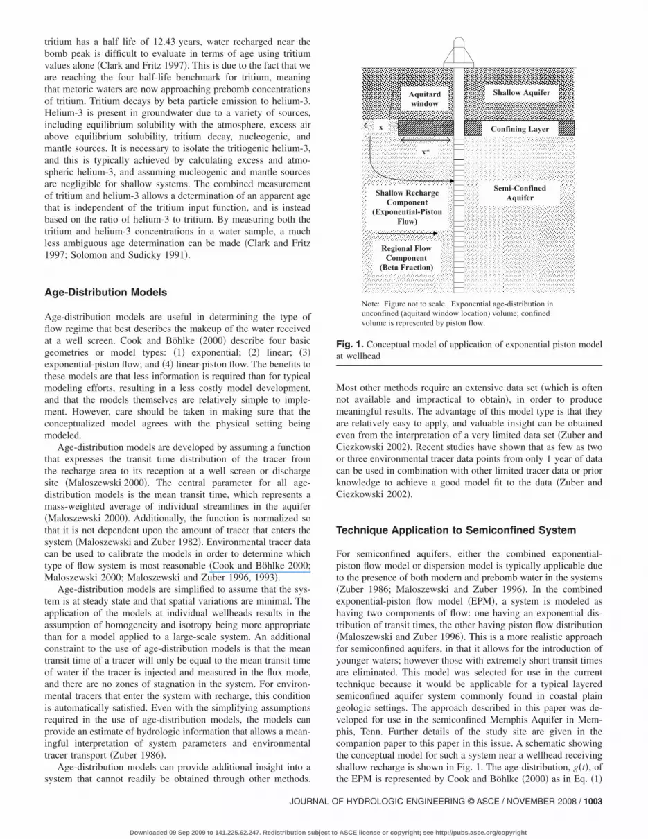
For semiconfined aquifers, either the combined exponential-piston flow model or dispersion model is typically applicable dueto the presence of both modern and prebomb water in the systems�Zuber 1986; Maloszewski and Zuber 1996�. In the combinedexponential-piston flow model �EPM�, a system is modeled ashaving two components of flow: one having an exponential dis-tribution of transit times, the other having piston flow distribution�Maloszewski and Zuber 1996�. This is a more realistic approachfor semiconfined aquifers, in that it allows for the introduction ofyounger waters; however those with extremely short transit timesare eliminated. This model was selected for use in the currenttechnique because it would be applicable for a typical layeredsemiconfined aquifer system commonly found in coastal plaingeologic settings. The approach described in this paper was de-veloped for use in the semiconfined Memphis Aquifer in Mem-phis, Tenn. Further details of the study site are given in thecompanion paper to this paper in this issue. A schematic showingthe conceptual model for such a system near a wellhead receivingshallow recharge is shown in Fig. 1. The age-distribution, g�t�, of
Semi-ConfinedAquifer
Shallow AquiferAquitardwindow
Shallow RechargeComponent
(Exponential-PistonFlow)
x*
Regional FlowComponent(Beta Fraction)
Note: Figure not to scale. Exponential age-distribution inunconfined (aquitard window location) volume; confinedvolume is represented by piston flow.
Confining Layerx
Fig. 1. Conceptual model of application of exponential piston modelat wellhead
the EPM is represented by Cook and Böhlke �2000� as in Eq. �1�
F HYDROLOGIC ENGINEERING © ASCE / NOVEMBER 2008 / 1003
ASCE license or copyright; see http://pubs.asce.org/copyright

g�t� =R
H�e��x*/x�−�tR/H��� for t �
H�x*
Rx�1�
where R=recharge through the confining unit breach �uniform,m/year�; H=aquifer thickness �ft�; �=constant porosity; t�transittime �year�; x=linear extent of recharge �ft�; and x*=distance tothe recharge source �ft�. The mean transit time, �, is then deter-mined from Eq. �2�, given by Cooke and Böhlke �2000�
� =H��x + x*�
Rx�2�
The appropriate age-distribution function for the model can beused in combination with tracer information to approximate pa-rameters for the flow system around a wellhead. The output tri-tium or helium-3 concentration for a water sample of mixed agein a system at steady state is determined from the use of theconvolution integral. Convolution integrals are useful in manyapplications where the response of a system at a specified time isdependent not only on its current state, but also on its past behav-ior �Boyce and DiPrima 1992�. This is the case for environmentaltracers, where the solution is dependent upon the past history oftracer input to the system. The convolution integral represents theinverse Laplace transform of the product of the transforms ofexpressions for the weighting, or system response, and input func-tions, as shown in Eqs. �3� and �4� �Boyce and DiPrima 1992�
H�s� = F�s�G�s� = L�h�t�� �3�
h�t� =�0
t
f�t − ��g���d� = L−1�H�s�� �4�
where F�s�=Laplace transform of known function f �input func-tion�; G�s�=Laplace transform of known function g �weighting orsystem response function�; and h�t�=convolution of f and g. Theexpression used for this research is given in Eq. �5�, as repre-sented by Cook and Böhlke �2000�
Cout�to� =�0
�
Cin�to − t�g�t�e−�tdt �5�
where Cin= input function for the environmental tracer; and�=decay constant of the radioactive tracer. In cases where anolder, tritium-free component of flow is known to contribute tothe sample, an additional parameter, �, is used with a specifiedbackground concentration of tritium, c�, and is added to the out-put concentration equation as given by Maloszewski and Zuber�1996� and shown in Eq. �6�
Cout�to� = �c� + �1 − ���0
�
Cin�to − t�g�t�e−�tdt �6�
where �=fraction of water that is tritium free; and c�=tritiumconcentration of the � fraction. Similarly, output concentrationsfor helium-3 can also be determined. Since helium-3 is producedby the beta decay of tritium, the equation is altered to account foringrowth, as shown in Eq. �7�
Cout�to� = �c� + �1 − ���0
�
Cin�to − t�g�t��1 − e−�t�dt �7�
The limits of integration for the convolution integrals arechosen based upon the tracer being used in the study. In the caseof tritium, it is acceptable to set the lower limit at a few years
prior to the increase in atmospheric tritium in the mid 1950s1004 / JOURNAL OF HYDROLOGIC ENGINEERING © ASCE / NOVEMBER
Downloaded 09 Sep 2009 to 141.225.62.247. Redistribution subject to
�Maloszewski and Zuber 2002�. The upper limit is set dependingupon the expected mean transit times, to include all input datathat might be contributing to the observed output concentrations.The upper limit can be determined experimentally by adjustingthe value until negligible changes are observed in the solutionswith the inclusion of additional years of input data �Zuber 1986�.
For most real-world situations, it is common to have dataavailable for the output concentration of environmental tracers,while certain input parameters are unknown. For such a case,the inverse problem is applied to determine appropriate parametervalues. Thus, for this research, an inverse solution procedure wasdeveloped so that the technique would be suitable for real-worldscenarios. It was assumed that for many cases, the parameters ofinterest �x ,x* ,� ,R� would be unknown, while measurements oftritium and helium-3 concentrations would be available for use ascalibration targets. Additionally, geochemical modeling �equilib-rium and mixing models� can be used to determine estimates ofshallow water contribution to production wells, via an aquitardwindow. This would allow an estimate of the � parameter to beused as prior information. The use of estimates of x* as priorinformation was also investigated, since locations of known sur-face or subsurface features that could provide pathways for hy-draulic communication might also be available.
Inverse Code Implementation
The inverse procedure used in this research was UCODE, a uni-versal inverse modeling code developed for the USGS by Poeterand Hill �1998�. UCODE is universal in that it can be applied toany application model, as long as specific instructions are fol-lowed for extracting parameter values and running the applicationmodel. This code was selected for incorporation into this studybecause it is freely available and widely used by many ground-water professionals. Nonlinear regression is used to solve the pa-rameter estimation problem by minimizing a weighted least-squares objective function. Weights reflecting measurement errorare assigned to observations and prior information by the user.The form of the objective function used in UCODE is given inEq. �8� �Hill 1998�
S�b� = �i=1
ND
�i�yi − yi��b��2 + �p=1
NPR
�p�Pp − Pp��b��2 �8�
where b=vector containing values of each of the parametersbeing estimated; ND=number of observations; NPR=number ofprior information values; yi= ith observation being matched by theregression; yi��b�=simulated value which corresponds to the ithobservation; Pp= pth prior estimate included in the regression;Pp��b�= pth simulated value; �i=weight for the ith observation;and �p=weight for the Pp= pth prior estimate �Hill 1998�.A modified Gauss–Newton method is employed within UCODEto adjust parameters to obtain a solution that minimizes theobjective function �Poeter and Hill 1998�. The modified versionof the Gauss–Newton method used in UCODE is also called aLevenberg–Marquardt method. The Marquardt parameter isadded to the regression to ensure that the parameter values used insuccessive iterations are better than the values in the previousiterations �Sun 1999�. A damping parameter is also incorporatedto damp oscillations and to make certain that maximum changesin parameter values remain within specified limits �Hill 1998�.The form of the modified Gauss–Newton method used in UCODE
is given in Eqs. �9� and �10� �Hill 1998�2008
ASCE license or copyright; see http://pubs.asce.org/copyright

�CTXrT�XrC + Imr�C−1dr = CTXr
T��y − y��br�� �9�
br+1 = rdr + br �10�
where r=parameter-estimation iteration number; Xr=sensitivitymatrix evaluated at parameter estimates br, with elements equalto �yi� /�bj; �=weight matrix; �XT�X�=symmetric, square matrixof dimension NP �number of parameters� by NP that is used tocalculate parameter statistics; C=diagonal scaling matrix with el-ement cjj equal to ��XT�X� j j�−1/2; dr=vector with the number ofelements equal to the number of estimated parameters; I=NP di-mensional identity matrix; y=observation being matched by theregression; y�=simulated value corresponding to the observation;mr=Marquardt parameter; and r=damping parameter �Hill1998�. An algorithm compatible with UCODE requirements waswritten to solve the convolution integral for this research.
Numerical integration was incorporated to solve for outputconcentration values of tritium and helium-3 to be compared withavailable observations. The mean age of the water sample, asgiven by Eq. �2�, was also computed for comparison with avail-able age measurements. The mean age and output tritium andhelium-3 concentrations were printed to a file for extraction byUCODE, so that parameter estimation iterations could be per-formed. A flowchart showing its connection to UCODE is shownin Fig. 2.
The numerical integration scheme employed within the age-distribution application model was the composite Simpson’s 1 /3rule for equally spaced data, appropriate for the annual data usedfor this model. An additional requirement of this technique is thatan even number of intervals be used in the approximation. Amethod with a lower error term was not necessary because of theanticipated accuracy limitations of the data to be used in themodel. Simpson’s 1 /3 rule and its associated error term are givenin Eqs. �11� and �12� �Hoffman 1992�
I = 1 h�fo + 4f1 + 2f2 + 4f3 + . . . + 4fn−1 + fn� �11�
Start
Initialize ProblemStart parameter estimation iterations, iteration# = 1
Create input files for the application model(s) using current parameter values
Execute application model(s)
Extract values from application output files anduse extracted values to calculate simulated equivalents of the observations
Start sensitivity loop, parameter# = 1
Perturb this parameter and recreate the input files for the application model(s)
Execute application model(s)
Extract values from application output files and use extracted valuesto calculate forward-difference sensitivities for this parameter
Unperturb this parameter
Last parameter?
Update parameter values using modified Gauss-Newton method
Converged or maximum numberof iterations?
Calculate sensitivities by central differencesCalculate and print statistics
Stop
iteration# = iteration# + 1
parameter# = parameter# + 1 NOYES
YES
NO
Fig. 2. Flowchart showing interaction between age-distributionalgorithm and UCODE
3
JOURNAL O
Downloaded 09 Sep 2009 to 141.225.62.247. Redistribution subject to
Error = O 1
n4 �12�
where h=interval spacing; fn=value of the function at point n;O represents a numerical coefficient for error associated withSimpson’s 1 /3 rule; and n=number of data points.
Synthetic Test Case
In order to evaluate the techniques capability of solving for vari-ous window recharge parameters, a synthetic test case was cre-ated. Thus, the system would be noise free and a demonstration ofperformance and utility could be assessed. The test case was de-veloped to evaluate the ability of the age-distribution inversemethod to estimate the window recharge rate �R�, distance to therecharge source �x*�, extent of recharge feature �x�, and fraction��� of submodern water comprising a sample from a well receiv-ing both modern and submodern components of flow, in a semi-confined aquifer. The test case was utilized to determine thenumber and type of observations required for a unique conver-gence. Additionally, it was important to evaluate the effect ofusing prior information available for certain parameters to deter-mine if this information was necessary for model convergence. Itwas also important to determine whether or not parameter estima-tion would be significantly improved with the use of prior infor-mation. The goal of the synthetic test case was to determine theminimum amount of data required to effectively use the techniquein a semiconfined aquifer setting, so that it could be applied byother investigators.
The test case used for evaluation of the current research meth-odology consists of a fully penetrating well screened in a semi-confined aquifer adjacent to a recharge source. A schematic of thesemiconfined aquifer test case is shown in Fig. 3. A forward
Semi-ConfinedAquifer
Shallow Aquifer
Confining Layer
x* = 914.4 m
Note: Figure not to scale. Exponential age-distribution inunconfined (aquitard window location) volume; confinedvolume is represented by piston flow.
x = 914.4 m
h = 106.68 mɛ = 0.39
R = 4.572 m/yr
Fig. 3. Semiconfined aquifer test case
model run for the application code was executed based on the
F HYDROLOGIC ENGINEERING © ASCE / NOVEMBER 2008 / 1005
ASCE license or copyright; see http://pubs.asce.org/copyright

selected test case parameters. Model estimates for tritium andhelium-3 were extracted from the output file, to be used as obser-vations in the subsequent inverse model runs. The results of theforward model run for the semiconfined aquifer test case areshown in Table 1. Various scenarios were tested to determine theamount of information available from the observations to estimateeach parameter. For scenario one, the inverse model only esti-mated the values of the window recharge and the extent of thewindow feature parameters �R ,x�. The next two scenarios wereconstructed to estimate three parameters each �x, R, � or x, x*, R�.The final scenario was created to estimate all four parameters ofinterest �R ,� ,x ,x*�. In the initial inverse model runs for the vari-ous scenarios, no error in the observations or prior informationon parameters was included. Additionally, a fairly large data set�n=15� was used as observation data.
Results
Search Parameter Sensitivities
The two-parameter model converged with errors of less than 1%regardless of the starting parameters, resulting in a unique solu-tion, as shown in Table 2. The standard error of the regressionwas very low, and the correlation coefficient was always nearlyequal to 1. The inverse models that were constructed to estimatethree or more parameters did not converge to a unique solutionwithout the inclusion of prior information. Model input valueswere varied by 10–30% percent of the known values, and solu-tions converged to values with associated errors as much as 25%.Composite scaled sensitivities were calculated within UCODE foreach model run, as shown in Fig. 4.
Model runs were next conducted using prior information on x*
and �. A unique calibration was achieved in both the three andfour parameter models by using prior information on � for themodel estimating x, R, �, and prior information on � and x* forthe four-parameter model. Convergence within 1% of known val-ues was achieved for the three-parameter model with prior infor-
Table 1. Forward Model Results for Semiconfined Aquifer Test Case
Observation dates andselected model outputa
Forwardmodel results
3H-2002 1.9183H-2000 1.8533H-1998 2.0543H-1996 2.5403H-1994 3.3113H-1992 4.3673H-1990 5.7073H-1988 7.3333H-1986 9.2433H-1984 11.4403H-1982 13.9183He-2002 5.4053He-2000 6.2063He-1998 7.2783He-1996 8.553
Mean age ��, years� 18.2a3H and 3He units are TU.
mation on �, regardless of starting parameters. The use of prior
1006 / JOURNAL OF HYDROLOGIC ENGINEERING © ASCE / NOVEMBER
Downloaded 09 Sep 2009 to 141.225.62.247. Redistribution subject to
information on x* did not allow a unique calibration to beachieved for the model estimating x, x*, R. For the four-parametermodel, convergence within 5% of known values was achieved,regardless of starting parameters, with the use of prior informa-tion on � and x*. When prior information on x* was removedfrom the four-parameter model, unique convergence was stillachieved, with the greatest error in parameter estimates being lessthan 6%. Although prior information was not specifically givenfor the values of x and x*, reasonable maximum and minimumvalues were entered into the model to limit the search space basedon known hydrologic and geologic data. The actual values for theobservation data are shown in Table 3, along with the modelestimates using prior information. The composite scaled sensitiv-ity of � increased by 92% with the addition of prior informationon the parameter, as shown in Fig. 5.
Table 2. Initial Model Results for Semiconfined Aquifer Test Case �NoObservation Errors or Prior Information Included�
Observation dates andselected model output
Forwardmodel results
Simulated values—model estimating
x, R
3H-2002 �TU� 1.918 1.9193H-2000 �TU� 1.853 1.8533H-1998 �TU� 2.054 2.0543H-1990 �TU� 5.707 5.7083H-1984 �TU� 11.440 11.4403He-2002 �TU� 5.405 5.4053He-2000 �TU� 6.206 6.2063He-1998 �TU� 7.278 7.278
x �m� 914.4 914.1
x* �m� 914.4 NAa
R �m/year� 4.572 4.573
� 0.75 NAa
Standard error of regression — 0.00352
r2 — 1.000aNA=not available.
0
10
20
30
40
50
60
x R
CompositeScaledSensitivity
0
10
20
30
40
50
60
x* x R
CompositeScaledSensitivity
(a.) Model estimating x, R (b.) Model estimating x*, x, R
0
10
20
30
40
50
60
x R B
CompositeScaledSensitivity
0
10
20
30
40
50
60
x x* R B
CompositeScaledSensitivity
(c.) Model estimating x, R, β (d.) Model estimating x, x*, R, β
Fig. 4. Composite scaled sensitivities for semiconfined aquifer testcase �no observation error, no prior information�
2008
ASCE license or copyright; see http://pubs.asce.org/copyright

Impact of Number of Observations
Once it had been determined that the method in this research wascapable of uniquely estimating all four parameters of interest, theremainder of the model runs were focused on this scenario, sinceall four parameters were likely to be of interest in future investi-gations. Subsequent model runs were developed to determine theminimum number of observations that would be required to esti-mate all four parameters, and the effect of observation error onthe resulting solutions. The effect of observation error was evalu-ated by introducing a random error to each observation thatranged from 0 to 10%. The upper limit of 10% was used becauseof the expected high accuracy and precision of the methods usedin determining the tritium and helium-3 values from field samplesin the Memphis aquifer. It should be noted that this value was
Table 3. Model Results for Semiconfined Aquifer Test Case �Prior Infor
Observation dates andselected model output
Forwardmodel results
Simulmod
3H-2002 �TU� 1.9183H-2000 �TU� 1.8533H-1998 �TU� 2.0543H-1990 �TU� 5.7073H-1984 �TU� 11.4403He-2002 �TU� 5.4053He-2000 �TU� 6.2063He-1998 �TU� 7.278
x �m� 914.4 9
x* �m� 914.4
R �m/year� 4.572
� 0.75
Standard error of regression —
r2 —
0
10
20
30
40
50
x R B
CompositeScaledSensitivity
0
10
20
30
40
50
x x* R B
CompositeScaledSensitivity
(c.) Model estimating x, x*, R, β
0
10
20
30
40
50
x* x R
CompositeScaledSensitivity
(a.) Model estimating x, R, β (b.) Model estimating x*, x, R
0
10
20
30
40
50
x x* R B
CompositeScaledSensitivity
(d.) Model estimating x, x*, R, β
(no prior on x*)
Fig. 5. Composite scaled sensitivities for semiconfined aquifer testcase �prior information included; no observation error�
JOURNAL O
Downloaded 09 Sep 2009 to 141.225.62.247. Redistribution subject to
chosen based upon values measured from the Memphis aquifer,and the precision could be less in hydrogeologic conditions dif-fering from the Mississippi Embayment, where geogenic sourcesof 3He may be much more significant. The conditions and preci-sion of the methodology are presented in detail by Bayer et al.�1989� and Solomon and Cook �2000�.
The model converged uniquely when estimating all four pa-rameters and the above described observation error was included.The values obtained from the model simulation including obser-vation error are shown in Table 4, along with the actual values forthe test case. Dimensionless sensitivities are shown in Table 5.
In the next set of model runs, observations were removed fromthe input data set in order to determine the minimum requireddata set. The observation data for tritium from 1984 and 1990were both removed, along with the observation for helium-3 in1998. These were removed because they represented older histori-cal data which carry a significant amount of information, but that
Included, No Observation Error�
alues—ating
Simulated values—model estimating
x, x*, �, R
Simulated values—model estimating
x, x*, �, R�no prior on x*�
1.919 1.919
1.853 1.853
2.054 2.055
5.708 5.709
11.440 11.441
5.405 5.405
6.207 6.207
7.278 7.278
868.7 968.7
867.1 969.1
4.573 4.573
0.750 0.750
53 0.00496 0.00387
0.998 0.998
Table 4. Model Results for Semiconfined Aquifer Test Case�Observation Error and Prior Information Included�
Observation dates andselected model output
Forwardmodel results
Simulated values—model estimating
x, x*, R, �
3H-2002 �TU� 1.918 1.9673H-2000 �TU� 1.853 1.9223H-1998 �TU� 2.054 2.1443H-1990 �TU� 5.707 5.8563H-1984 �TU� 11.440 11.6063He-2002 �TU� 5.405 5.7623He-2000 �TU� 6.206 6.6183He-1998 �TU� 7.278 7.736
x �m� 914.4 916.6
x* �m� 914.4 933.9
R �m/year� 4.572 4.414
� 0.75 0.750
Standard error of regression — 0.18420
r2 — 0.998
mation
ated vel estimx, R, �
1.919
1.853
2.054
5.708
11.440
5.405
6.206
7.278
14.1
NA
4.573
0.750
0.003
1.000
F HYDROLOGIC ENGINEERING © ASCE / NOVEMBER 2008 / 1007
ASCE license or copyright; see http://pubs.asce.org/copyright

are less likely to exist in typical settings. It was important withinthis research to identify minimum data requirements for success-ful model calibration. The models resulted in a unique solutionregardless of starting parameters; however, the loss of the obser-vation data from the earlier years resulted in reduced compositescaled sensitivities for the parameters, and increased error in theparameter estimates. This is due to the fact that a large amount ofinformation for estimating x, x*, and � had previously been ob-tained through the tritium observations from 1984 and 1990. Thegreatest contribution for the estimate of R had been obtained fromthe helium observation from 1998, which was also removed forthis simulation. The simulations were run with and without obser-vation error. The observation error had a greater effect on themodel with fewer observation points than it had with that con-taining the early-year data. The model results from the simula-tions with the early-year observation data removed are shown inTable 6. Dimensionless scaled sensitivities are shown in Table 7.
An evaluation of sensitivities indicated that, as with previousmodel runs, the greatest amount of information from the observa-tions was available for the estimation of x and x*, while the leastamount of information was available for �. The helium-3 obser-vation from 2000 provided the most information toward the esti-mation of all four parameters. A final set of model scenarios wasevaluated to determine the impact of removing an additional tri-tium or helium-3 observation. If starting parameters were fairlyclose to the true values �within 15%�, models converged to valuesthat were within about 5% of actual parameter values. However,if starting parameters were much different than actual values, themodels converged to parameter values that had very large �more
Table 5. Dimensionless Scaled Sensitivities for Semiconfined AquiferTest Case �Observation Error and Prior Information Included�
Observationdate x* x � R
3H-2002 14.3 −14.3 −7.07 −6.213H-2000 13.9 −14.0 −6.89 −7.723H-1998 15.7 −15.7 −7.78 −9.573H-1990 44.8 −45.0 −22.6 −18.93H-1984 90.0 −90.3 −45.6 −28.03He-2002 44.1 −44.2 −22.2 −35.43He-2000 50.8 −51.0 −25.7 −40.63He-1998 59.6 −59.8 −30.1 −45.6
Table 6. Model Results for Semiconfined Aquifer Test Case �Early Obse
Observation dates andselected model output
Forwardmodel results
3H-2002 �TU� 1.9183H-2000 �TU� 1.8533H-1998 �TU� 2.0543He-2002 �TU� 5.4053He-2000 �TU� 6.206
x �m� 914.4
x* �m� 914.4
R �m/year� 4.572
� 0.75
Standard error of regression —
r2 —
1008 / JOURNAL OF HYDROLOGIC ENGINEERING © ASCE / NOVEMBER
Downloaded 09 Sep 2009 to 141.225.62.247. Redistribution subject to
than 50%� errors in the estimate of x. Thus, a unique convergencewas not achieved when additional tritium or helium values wereremoved, indicating that a minimum required data set had beenidentified.
Results of the test case runs, as shown in Tables 2–7, indicatethat it is not necessary to have a long record of tritium inputvalues for the estimation of all four parameters in question�R ,� ,x ,x*�, as long as helium-3 measurements and prior infor-mation on � are available. It is not possible to uniquely determinethe four parameters without the combination of tritium andhelium-3 values. Because helium-3 is the daughter product oftritium decay, the concurrent measurements provide a great dealof information as to the age of the water, which restricts thepossible solutions. Without the information provided by helium-3,the solution cannot be determined because the concentrationscould be observed in several types of flow regimes. Helium-3observations pinpoint whether the system in question has rapid orslow turnover times, thus marking the point in time at whichrecharge occurred.
Discussion
Data Requirements and Model Convergence
For the test case, a minimum of two helium-3 measurements, andthree tritium measurements were required for a unique solutionwhen estimating all four parameters. This represents data col-lected over only 3 years. This makes this approach very attrac-tive, in that a minimal amount of observation data is required. In
n Data Removed�
Simulated values—del estimating x, x*, R, ��no observation error�
Simulated values—model estimating x, x*, R, ��observation error included�
1.939 2.064
1.842 1.969
2.026 2.172
5.408 5.854
6.210 6.726
914.5 818.2
835.1 937.3
4.733 4.673
0.750 0.750
0.0215 0.0841
0.999 0.999
Table 7. Dimensionless Scaled Sensitivities for Semiconfined AquiferTest Case �Early Observation Data Removed; No Observation Error�
Observationdate x* X � R
3H-2002 17.6 −17.3 −7.46 −7.203H-2000 16.7 −16.5 −7.08 −8.863H-1998 18.6 −18.3 −7.89 −11.03He-2002 52.5 −51.6 −22.6 −38.93He-2000 60.5 −59.5 −26.1 −45.2
rvatio
mo
2008
ASCE license or copyright; see http://pubs.asce.org/copyright

many cases, a good portion of this data may already exist, requir-ing the collection of only a small amount of additional data inorder to apply the technique.
Convergence problems can occur if composite scaled sensitivi-ties for any parameter are less than about 0.01 times the largestsensitivity value �Poeter and Hill 1998�. This difficulty was notencountered in any of the model scenarios tested. The compositescaled sensitivities for the various model types indicate that thetritium and helium-3 observation data provide the most informa-tion toward estimating x and x*, and the least amount of informa-tion in the estimation of the � parameter. Dimensionless scaledsensitivities provide information about the importance of eachobservation to each of the parameters. In general, the early-yeartritium and helium-3 data provided more information for the es-timation of the parameters. Tritium observation data from the1980s and early 1990s in the test case yielded much higher di-mensionless scaled sensitivity values for x, x*, and �. This is dueto the variability of the tritium input function, and its continueddecline from peak values after the ban on above ground nuclearweapons testing. Observations from these years would have re-charge components with a much stronger tritium signal, thus theinformation provided by these values is less ambiguous than tri-tium observations from more recent years. It should be noted thatan independent estimation of � may be used to constrain theinverse model by comparing the tritium value from the 3H / 3He tothe tritium input function �Manning et al. 2005�. This may pro-vide further stability in the overall estimation of the remainingparameters.
Helium-3 observations were only used in the test case for theyears 1998, 2000, and 2002. This is due to the fact that the tech-nique of age dating with tritium/helium-3 is relatively new, so it isunlikely that data would actually be available for helium-3 foryears prior to the mid 1990s. Thus, simulations were performedfor the test case with only the observations that were likely toexist in real-world scenarios. Regardless, the helium-3 valuesfrom all three dates provided a significant amount of informationto the estimation of the parameters, with all four values havinghigh dimensionless scaled sensitivities to helium-3 observations.As the tritium signal continues to decay, it will become increas-ingly important to collect combined tritium/helium-3 data toavoid ambiguity from a weak tritium signal.
Impact of Prior Information
The test case results also indicate that it is important to have priorknowledge about the composition of the water sample in terms ofthe percentage of submodern water. Prior information on � im-proved the regression significantly. This type of information canreadily be estimated using major ion water chemistry and freeequilibrium geochemical and mixing software, such as NETPATH�Plummer, et al. 1991�, to determine the percentage of shallowwater and unaffected semiconfined aquifer water that comprise aparticular sample. In the test case, a lower weight indicative of astandard deviation of 10% was applied to the prior informationfor the � parameter. This weight was applied so that the modelwas allowed to converge to � values within the range of expectedaccuracy of the estimate, rather than being required to converge toa specific value of �.
Prior information on x* did little to improve the regressionresults, as shown in Tables 2–7 and Figs. 4 and 5. This is mainlydue to the fact that observation data already provided a significantamount of information toward the estimation of that parameter.
The additional information provided by the prior information onlyJOURNAL O
Downloaded 09 Sep 2009 to 141.225.62.247. Redistribution subject to
reduced errors by about 1%. Because prior knowledge about thelocation of the recharge source is not required, the applicability ofthis method is broadened to incorporate systems where little hy-drogeologic information is available. It is much more expensiveto obtain the data necessary to identify sources of recharge toserve as prior information, whereas it is relatively inexpensiveto collect geochemical data in order to obtain prior informationon �. Although prior information was not specifically given forthe values of x and x*, it is necessary to constrain the search spaceto reasonable maximum and minimum values based on knownhydrologic and geologic data.
Conclusions
Several conclusions can be drawn from the results of this inves-tigation. The EPM, when used in combination with environmentaltracer data and geochemical information, is capable of identifyingthe location of a source of recharge to a well screened in a semi-confined aquifer. Using two helium-3 measurements and threetritium measurements, all four parameters of interest: �1� linearextent of recharge region �x�; �2� distance from the well to therecharge source �x*�; �3� fraction of tritium free water ���; and �4�the recharge flux �R�, can be uniquely determined in the presenceof observation error as long as prior information is available for�; however, it is not necessary to have prior information on x* fora unique solution to be obtained. Additionally, the number andtype of observations �tritium or helium-3� available for calibrationhave a direct impact on the ability of the technique to converge toa unique solution.
The benefit of this technique is that recharge locations can bereliably identified with only a small amount of observation data.The minimal data requirement makes the technique unique, inthat most modeling efforts require extensive data sets over longperiods of record. The results of this study as applied to wellheadsscreened in the Memphis aquifer in Memphis, Tenn., will be pre-sented in a subsequent paper. The study will demonstrate howmultiple wells may be used in conjunction to identify the mostprobable locations of leakage features.
Acknowledgments
The research conducted for this publication was funded by theGround Water Institute at The University of Memphis. The writ-ers wish to express their gratitude to the Ground Water Instituteand its funding partners for making this work possible.
Notation
The following symbols are used in this paper:b � vector containing values of each of parameters
being estimated;C � diagonal scaling matrix;
Cin�t� � input function for environmental tracer;Cout � output concentration of environmental tracer;
c � tritium concentration;dr � vector with number of elements equal to number
of estimated parameters;F�s� � Laplace transform of known input function;G�s� � Laplace transform of known system response
function;
F HYDROLOGIC ENGINEERING © ASCE / NOVEMBER 2008 / 1009
ASCE license or copyright; see http://pubs.asce.org/copyright

g�t� � age-distribution function;H � aquifer thickness;
H�s� � system response function;h�t� � input function;
mr � Marquardt parameter;ND � number of observations;
NPR � number of prior information values;Pp � Pth prior estimate included in regression;
Pp��b� � pth simulated value;R � recharge through confining unit breach;R � parameter estimation interation number;T � mean transit time;t � transit time;
Xr � sensitivity matrix evaluated at parameter estimates;�XT�X� � matrix used to calculate parameter statistics;
x � linear extent of recharge;x* � distance to recharge source;yi � ith observation being matched by regression;
yi��b� � simulated value which corresponds to ithobservation;
� � fraction of water that is tritium free;� � constant porosity;� � decay constant of radioactive tracer; � damping parameter;
�i � weight for ith observation; and�p � weight for pth prior estimate.
References
Bayer, R., Schlosser, P., Bönisch, G., Rupp, H., Zaucker, R., and Zimmer,G. �1989�. “Performance and blank components of a mass spectromet-ric system for routine measurements of helium isotopes and tritium bythe 3He ingrowth method.” Sitzungsberichte der Heidelberger Akad-emie der Wissenschaften, Mathematisch-NaturwissenschaftlicheKlasse, 5. Anhandlung, Springer, Berlin, 240–279.
Beyerle, U., Aeschbach-Hertig, W., Hofer, M., Imboden, D. M., Baur, H.,and Kipfer, R. �1999�. “Infiltration of river water to a shallow aquiferinvestigated with 3H / 3He, noble gases, and CFCs.” J. Hydrol.,220�3�, 169–185.
Boyce, W. E., and DiPrima, R. C. �1992�. Elementary differential equa-tions, Wiley, New York.
Carmi, I., and Gat, J. �1994�. “Estimating the turnover time of ground-water reservoirs by the helium-3/tritium method in the era of declin-ing atmospheric tritium levels: Opportunities and limitations in thetime bracket 1990–2000.” Isr. J. Earth Sci., 43, 249–253.
Clark, I., and Fritz, P. �1997�. Environmental isotopes in hydrogeology,CRC, Boca Raton, Fla.
Clark, J. F., Hudson, G. B., Davisson, M. L., Woodside, G., and Herndon,R. �2004�. “Geochemical imaging of flow near an artificial rechargefacility, Orange County, California.” Ground Water, 42�2�, 167–174.
Cook, P. G., and Böhlke, J. �2000�. “Determining timescales for ground-water flow and solute transport.” Environmental tracers in subsurfacehydrology, P. Cook and A. Herczeg, eds., Kluwer Academic, Boston.
Ekwurzel, B., Schlosser, P., Smethie, W. M., Jr., Plummer, L. N.,Busenberg, E., Michel, R. L., Weppernig, R., and Stute, M. �1994�.“Dating of shallow groundwater: Comparison of the transient tracers3H / 3He, chlorofluorocarbons, and 85Kr.” Water Resour. Res., 30�6�,1693–1708.
Hill, M. C. �1998�. “Methods and guidelines for effective model calibra-tion.” U.S. Geological Survey Water-Resources Investigations Rep.
No. 98-4005, Denver.1010 / JOURNAL OF HYDROLOGIC ENGINEERING © ASCE / NOVEMBER
Downloaded 09 Sep 2009 to 141.225.62.247. Redistribution subject to
Hoffman, J. D. �1992�. Numerical methods for engineers and scientists,McGraw-Hill, New York.
Maloszewski, P. �2000�. “Lumped-parameter models as a tool for deter-mining the hydrological parameters of some groundwater systemsbased on isotope data.” Tracers and modeling in hydrogeology, IAHSPublication No. 262, Vienna, Austria, 271–276.
Maloszewski, P., and Zuber, A. �1982�. “Determining the turnover timeof groundwater systems with the aid of environmental tracers. I: Mod-els and their applicability.” J. Hydrol., 57, 207–231.
Maloszewski, P., and Zuber, A. �1993�. “Principles and practice of cali-bration and validation of mathematical models for the interpretationof environmental tracer data in aquifers.” Adv. Water Resour., 16,173–190.
Maloszewski, P., and Zuber, A. �1996�. “Lumped parameter models forthe interpretation of environmental tracer data.” Manual on math-ematical models in isotope hydrogeology, IAEA-TECDOC-910, 28,No. 6, International Atomic Energy Agency, Vienna, Austria.
Maloszewski, P., and Zuber, A. �2002�. “Manual on lumped parametermodels used for the interpretation of environmental tracer data ingroundwaters.” Use of isotopes for analyses of flow and transportdynamics in groundwater systems. Results of a coordinated researchproject 1996–1999, International Atomic Energy Agency, Vienna,Austria.
Manning, A. H., Solomon, D. K., and Thiros, S. A. �2005�. “3H/3He agedata in assessing the susceptibility of wells to contamination.” GroundWater, 43�3�, 353–367.
Plummer, L. N., Prestemon, E. C., and Parkhurst, D. L. �1991�. “Aninteractive code �NETPATH� for modeling NET geochemical reac-tions along a flow PATH.” U.S. Geological Survey Water-ResourcesInvestigations Rep. No. 91-4078, Reston, Va.
Poeter, E. P., and Hill, M., C. �1998�. “Documentation of UCODE, Acomputer code for universal inverse modeling.” U.S. Geological Sur-vey Water-Resources Investigations Rep. No. 98-4080, Denver.
Robertson, W. D., and Cherry, J. A. �1989�. “Tritium as an indicator ofrecharge and dispersion in a groundwater system in central Ontario.”Water Resour. Res., 25�6�, 1097–1109.
Shapiro, S. D., Rowe, G., Schlosser, P., Ludin, A., and Stute, M. �1998�.“Tritium-helium 3 dating under complex conditions in hydraulicallystressed areas of a buried-valley aquifer.” Water Resour. Res., 34�5�,1165–1180.
Solomon, D. K., and Cook, P. G. �2000�. “3H and 3He.” Environmentaltracers in subsurface hydrology, P. G. Cook and A. L. Herczeg, eds.,Kluwer, Boston, 397–424.
Solomon, D. K., Poreda, R. J., Cook, P. G., and Hunt, A. �1995�. “Sitecharacterization using 3H / 3He ground-water ages, Cape Cod, MA.”Ground Water, 33�6�, 988–996.
Solomon, D. K., Schiff, S. L., Poreda, R. J., and Clarke, W. B. �1993�.“A validation of the 3H / 3He method for determining groundwaterrecharge.” Water Resour. Res., 29�9�, 2951–2962.
Solomon, D. K., and Sudicky, E. A. �1991�. “Tritium and helium 3 iso-tope ratios for direct estimation of spatial variations in groundwaterrecharge.” Water Resour. Res., 27�9�, 2309–2319.
Sun, N. Z. �1999�. Inverse problems in groundwater modeling, KluwerAcademic, Norwell, Mass.
Zuber, A. �1986�. “Mathematical models for the interpretation of envi-ronmental radioisotopes in groundwater systems.” Handbook of envi-ronmental isotope geochemistry, P. Fritz and J. Ch. Fontes, eds., Vol.2, Elsevier Science, New York.
Zuber, A., and Ciezkowski, W. �2002�. “A combined interpretation ofenvironmental isotopes for analyses of flow and transport parametersby making use of the lumped-parameter approach.” Use of isotopesfor analyses of flow and transport dynamics in groundwater systems.Results of a coordinated research project 1996–1999, InternationalAtomic Energy Agency, Vienna, Austria.
2008
ASCE license or copyright; see http://pubs.asce.org/copyright


