AES 30th International Conference, Saariselkä, Finland, 2007 March 15–17 1

INVESTIGATION OF THE PERCEIVED SPATIAL RESOLUTION OF HIGHER ORDER AMBISONICS SOUND FIELDS: A SUBJECTIVE

EVALUATION INVOLVING VIRTUAL AND REAL 3D MICROPHONES

STÉPHANIE BERTET13, JÉRÔME DANIEL1, ETIENNE PARIZET2, LAËTITIA GROS1 AND OLIVIER WARUSFEL3

1 France Telecom R&D, 2 avenue Pierre Marzin, 22307 Lannion Cedex, France stephanie.bertet@orange-ftgroup.com

2 Laboratoire Vibrations Acoustique, Insa Lyon,France 3 Dept. acoustique des salles, Institut de recherche et coordination acoustique / musique (IRCAM), Paris, France

Natural sound field can be reproduced through loudspeakers using ambisonics and Higher Order Ambisonics (HOA) microphone recordings. The HOA sound field encoding approach is based on spherical harmonics decomposition. The more components used to encode the sound field, the finer the spatial resolution is. As a result of previous studies, two HOA (2nd and 4th order) microphone prototypes have been developed. To evaluate the perceived spatial resolution and encoding artefacts on the horizontal plane, a localisation test was performed comparing these prototypes, a SoundField microphone and a simulated ideal 4th order encoding system. The HOA reproduction system was composed of twelve loudspeakers equally distributed on a circle. Thirteen target positions were chosen around the listener. An adjustment method using an auditory pointer was used to avoid bias effects of usual reporting methods. The human localisation error occurring for each of the tested systems has been compared. A statistical analysis showed significance differences when using the 4th order system, the 2nd order system and the SoundField microphone.

INTRODUCTION

Nowadays, techniques exist to recreate a sound field in three dimensions, either reproducing a natural sound field or using virtual sources. One of these techniques is Higher Order Ambisonics (HOA). Based on spherical harmonics sound field decomposition, it provides a hierarchical description of a natural or simulated sound field. This approach presents advantages like sound field manipulations (rotation) and scalability of the reproduced sound field depending on the restitution system. The first ambisonic order involves the omni and bidirectional components (first harmonics). Higher order encoding systems involve second and higher harmonics. France Telecom R&D has developed two HOA microphone prototypes [1] currently effective for spatial recording of natural sound field. They consist of 32 (or 12) acoustic sensors distributed on the surface of a rigid sphere giving a fourth order (or second order) ambisonic encoding system. These prototypes have been validated with objective measurements and compared to theoretical encoding [2], [3]. Currently the

practical utilisation is still confronted with some questions. What is the real contribution of high order components? How can we quantify the perceived resolution? Are the HOA microphones encoding equivalent to an “ideal encoding” from a subjective point of view? To evaluate spatial audio reproduction techniques, different criteria can be explored. Among others, the spatial resolution of the reproduced sound field can be linked with the capacity of a listener to locate a sound source in the reproduced sound scene. Therefore a subjective test was conducted to evaluate how precisely a listener can localise sound sources encoded with five encoding systems of various complexity.

1 HIGH ORDER AMBISONIC SYSTEMS

The ambisonic concept was initiated thirty years ago by D. Cooper [4] , J. Gibson [5] and Michael Gerzon [6] among others. It is based on a spherical harmonics decomposition to reproduce a sound field in an area around the sweet spot. The decomposition includes two steps: the encoding and the decoding process.

BERTET et al. Investigation of the perceived spatial resolution of HOA sound fields

AES 30th International Conference, Saariselkä, Finland, 2007 March 15–17 2

1.1 Encoding process

The sound pressure can be expressed as a Fourier-Bessel decomposition in a spherical coordinate basis:

0 0 1( , , ) ( ) ( , )

mm

m mn mnm n

p kr i j kr B Yσ σ

σθ δ θ δ

∞

= = =±

= ∑ ∑∑ (1)

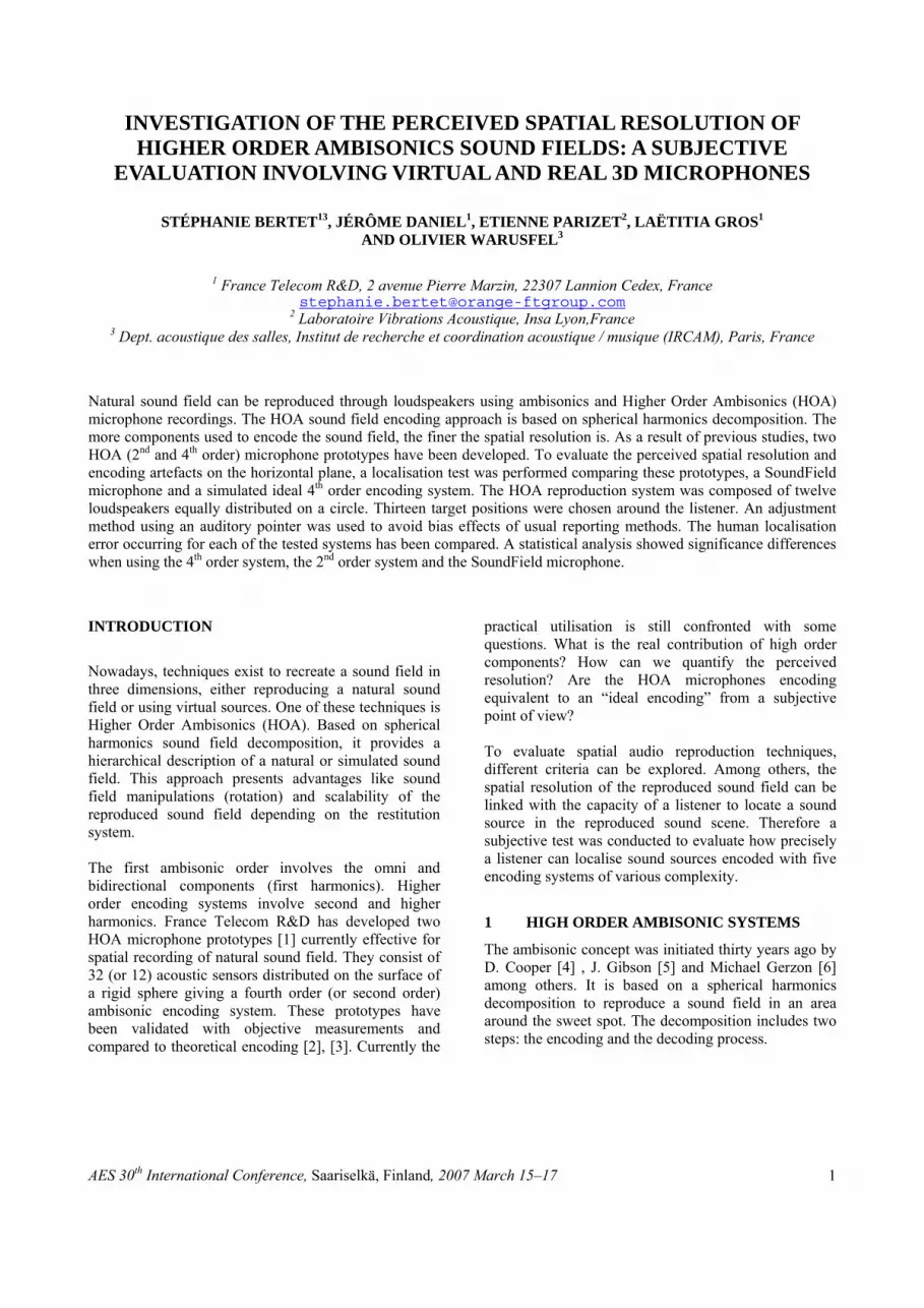
The mnY σ components represent the spherical harmonics basis where θ is the azimuth angle and δ the elevation angle with the harmonic order m, n ≤ m, and σ = ±1. The jm(kr) functions are the spherical Bessel functions where kr is the wave number. Each mnBσ component ensues from the orthogonal projection of the acoustical pressure p on the corresponding spherical harmonic. The theoretical Fourier Bessel decomposition of equation (1) includes an infinite number of harmonics. Practically, the sound pressure decomposition is truncated to an M order. Theoretically, the higher the order M is, the finer the encoded sound field is. Figure 1 shows the directivity pattern for a zero, first and second order components for a horizontal encoding. Two sources (θv’ and θv) quite close to each other are more discriminated with the second order coefficients than with the first order ones only. When synthesizing virtual environments, the HOA components are easily built. On the other hand, when recording a real environment, at least (M + 1)2 sensors are needed [2], which can induce practical limitations of the microphone structure (more detailed in 3.1) and physical limitations regarding the sensors themselves (impulse responses, similarity between sensors).

W

X

Y

θv

θv'

U V

Figure 1: Horizontal encoding using 0th, 1st order (left) and 2nd order (right) directivity patterns. Positive and

negative gains are resp. in red and blue. For each source (displayed with the arrow) and each directivity, the

encoding gain is given by the intersection point between arrows and patterns (more precisely its distance from

the centre).

1.2 Decoding process

The decoding process reconstructs the encoded sound field in a listening area depending on the loudspeaker setup. Typically, it consists of matrixing the HOA signals to produce the loudspeaker signals. The number of required loudspeakers depends on the order of the ambisonic scene to be reproduced. For an Mth encoding order, at least N=2M+2 loudspeakers are recommended for a homogeneous reproduction in the horizontal plane [7]. Therefore, the reproduction system can be a limitation if the number of loudspeakers is not sufficient for playing back the HOA encoded signals. Moreover, the listening area where an accurate rendering is achieved gets smaller with increasing frequency and decreasing ambisonic order. Therefore, for low ambisonic order this listening area is even smaller than a listener’s head at high frequency, meaning that even for a single listener situated at the sweet spot the sound field is not entirely reconstructed. Three kinds of decoding matrix are known and can be combined [3]. The “basic” one applies gains such that the reproduced ambisonic sound field would be the same as a sound field recorded at the listening position. As said before the sound field reconstruction is dependent on frequency. Therefore the decoded sound field is well reconstructed up to a limit frequency, increasing with the HOA order. In order to optimise the reconstruction in high frequencies the so-called “max rE” decoding aims at “concentrating” the energy contributions towards the expected direction [3]. The “in-phase” decoding process is recommended to reproduce the ambisonic sound field in a large listening area.

Acoustic space for recording (a) or Virtual

sources (b)

Spatial encoding

Spherical harmonics basis

Spatial decoding

Reproduction acoustic space

(a) p signals (b) sources signal Sv, with

an azimuth angle θv

Encoding gains c

Spatial components HOA mnBσ

Decoding matrix D

BERTET et al. Investigation of the perceived spatial resolution of HOA sound fields

AES 30th International Conference, Saariselkä, Finland, 2007 March 15–17 3

2 SOUND LOCALISATION

2.1 Sound localisation studies

Localisation has been studied for decades either in real conditions or with a reproduced sound field. In the horizontal plane the minimum localisation blur occurs from sources in front of the subject [8]. In that case the source discrimination varies from ±1° to ±4°. These variations could be due to the test signals (sinusoids, impulses, broadband noise) according to the published studies. For other source directions the localisation accuracy is reduced: e.g. localisation blur using white noise pulses varies from ± 5.5° [8] to ±10° [9] behind the subject. Such discrepancies between studies could be related to the measurement device (i.e. the device used by the subject to report his answer).

2.2 Reporting methods

Evaluating sound localisation is not an easy task. The reporting method should introduce as little bias as possible in the test to be valid. A great number of techniques were used. The absolute judgment technique used by Wightman [10] and Wenzel et al. [11] was a naming method. After a 10 hours training session the subject had to give the azimuth and elevation estimates of the heard target. Besides this long training session, a drawback of this method was that another person had to report the answers and errors could be introduced. Makous & Middlebrooks [9] and Bronkhorst [12] used a head tracker. The listener had to point the target with the head. This method needed a short training but the time lag between the sound presentation and the subject’s movement, as well as the fact that no feedback was given to him could have induced errors especially behind the listener. Seeber [13] used a visual pointer. The listener had to match a light placed at the same distance as the loudspeaker setup with the target sound. However, in order to obtain a simultaneous response to the stimulus such a device can be used for frontal localisation only. Moreover, there can be a bias when a subject has to describe an auditory sensation with a visual one [14]. A way to remove this bias is to use a sound instead of a light. Preibisch-Effenberger in [8] and Pulkki and Hirvonen [15] used an auditory pointer with an adjustment method. The target was the tested signal and the pointer an independent loudspeaker mounted on a rotating arm controlled by a rotating button. This last method was chosen for our experiment.

3 THE EXPERIMENT

3.1 The tested systems

Five systems were tested: - the SoundField, first order ambisonic microphone, - a second order microphone prototype, denoted in the

following as the 12 sensors - a fourth order microphone prototype (the 32

sensors), - a third order system constituted by the 8 sensors

placed in the horizontal plane of the 32 sensors microphone (the 8 sensors),

- a theoretical fourth order encoding system, considered as the reference (ideal 4th order).

In the experiment, the impulse responses of each system have been considered to generate the stimuli. Then, the three ambisonic microphones, the SoundField microphone and the two HOA microphone prototypes were measured at IRCAM in the anechoic chamber. The measures were sampled from -40° to 90° in elevation and from 0° to 360° in azimuth with a 5° step. The procedure is detailed in [2]. The impulse responses of the measured microphones in the horizontal plane were linearly interpolated every degree. These responses were used to characterise the actual directional encoding of the 32 sensors, 12 sensors and 8 sensors systems. The impulse responses of the SoundField microphone were measured in B-format (W, X, Y, Z signals).

3.1.1 The SoundField microphone

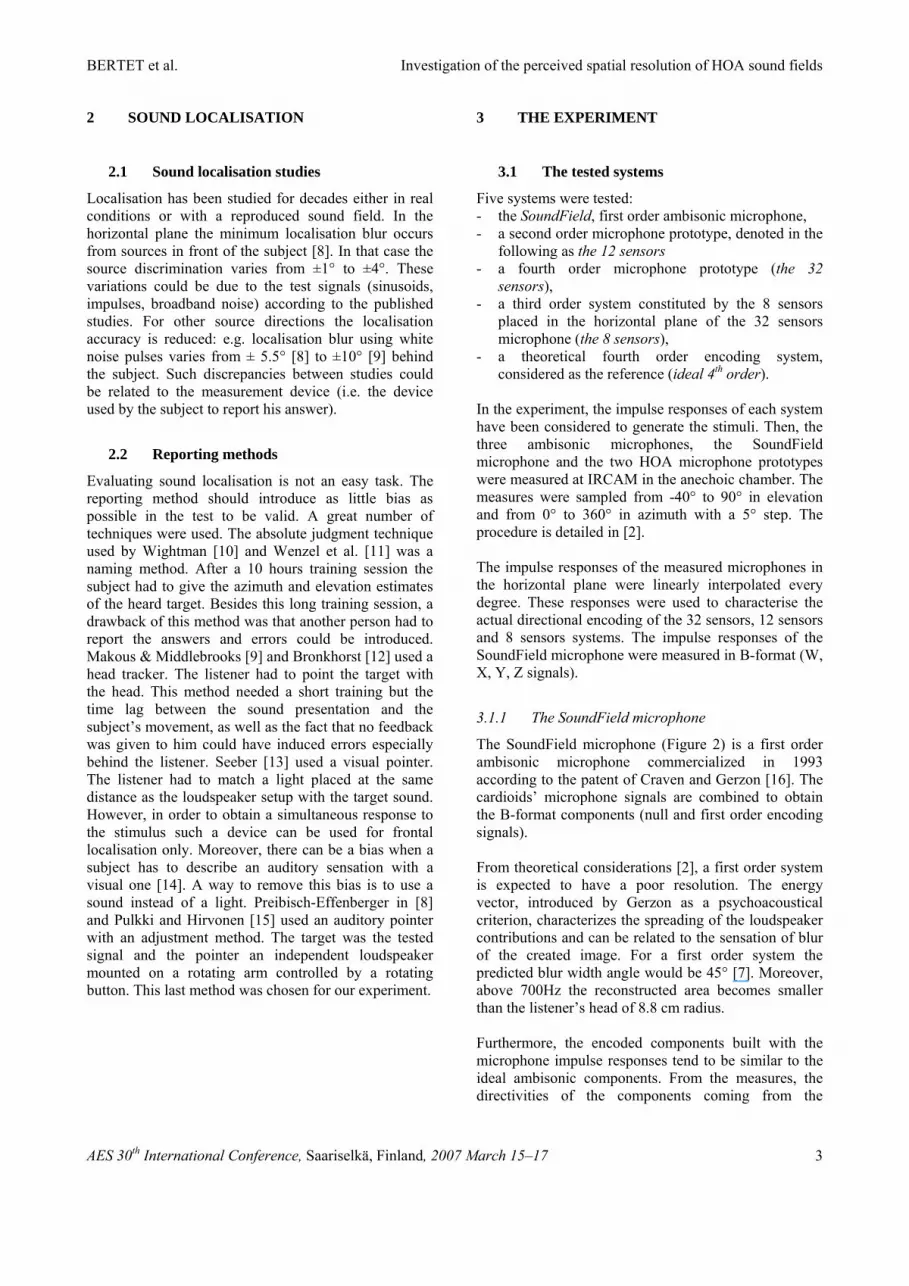
The SoundField microphone (Figure 2) is a first order ambisonic microphone commercialized in 1993 according to the patent of Craven and Gerzon [16]. The cardioids’ microphone signals are combined to obtain the B-format components (null and first order encoding signals). From theoretical considerations [2], a first order system is expected to have a poor resolution. The energy vector, introduced by Gerzon as a psychoacoustical criterion, characterizes the spreading of the loudspeaker contributions and can be related to the sensation of blur of the created image. For a first order system the predicted blur width angle would be 45° [7]. Moreover, above 700Hz the reconstructed area becomes smaller than the listener’s head of 8.8 cm radius. Furthermore, the encoded components built with the microphone impulse responses tend to be similar to the ideal ambisonic components. From the measures, the directivities of the components coming from the

BERTET et al. Investigation of the perceived spatial resolution of HOA sound fields

AES 30th International Conference, Saariselkä, Finland, 2007 March 15–17 4

SoundField signals showed a good reconstruction up to 10 kHz.

3.1.2 The 2nd and 4th order microphone prototypes

In order to get higher precision in the reproduced sound field, high order components have to be involved in the encoded sound field reconstruction. By adding high order components the resolution is expected to be better. The blur width angle is predicted to be 30° for a second order encoding system, 22.5° for a third order encoding system and 18° for a fourth order encoding system. Moreover, the limit frequency (above the reconstructed area becomes smaller than a listener’s head) is expected to be 1300 Hz for a second order encoding system, 1900 Hz for a third order encoding system and 2500 Hz for a fourth order encoding system. Considering the construction of a microphone, a compromise has to be made between the decomposition order (number of sensors giving (M+1)2 components), the aliasing frequency (related to the width of the structure) and the orthonormality properties (imposing the sensors position). France Telecom has developed two HOA microphones of second and fourth order (Figure 2). The sensors of the second order microphone are placed on a dodecahedron configuration on a semi rigid sphere (plastic ball) of 7cm diameter. The 32 sensors of the fourth order microphone are placed on a regular pentaki dodecahedron configuration on a sphere similar to the second order one [2]. For these two microphones, the greater space between sensors generated a lower aliasing frequency than the SoundField microphone (6 kHz for the 12 sensors, 8 kHz for the 32 sensors) imposing signal filtering in order to get a better sound field reconstruction [2]. For this test a filter matrix is applied to the measures, minimising the reconstruction errors. This encoding allows a limit frequency of reconstruction around 15kHz.

Figure 2: Soundfield microphone (left) composed by four coincident cardioids sensors. Second order

ambisonic microphone prototype (middle) composed by 12 sensors positioned in dodecahedron configuration. Fourth order ambisonic microphone prototype (right)

composed by 32 sensors positioned in pentaki dodecahedron configuration.

The 8 sensors encoding system is evaluated to measure the influence of the sensors placed off the horizontal plane for a horizontal restitution.

3.2 Restitution system

The HOA order determines the number of loudspeakers needed [3]. At least 2M+2 loudspeakers are needed to reproduce an Mth Ambisonic order encoding sound field in 2-D. In our study, twelve Studer loudspeakers evenly distributed on a regular dodecagonal structure composed the HOA reproduction system (Figure 3). In order to optimize the restitution, two decoding processes (basic and maxrE decoding) are combined. The crossover frequency depended on the order of the system (according to the limit frequencies of the acoustic reconstruction at centred listener ears [2]). The setup was located in a room composed of absorbent wall panels and ceiling at France Telecom R&D. The room reverberation time was 0.3s for frequencies below 500Hz and 0.2s above.

3.3 The pointing method

It was decided to use an acoustic pointer as in the study from Pulkki and Hirvonen [15] though in a reverse configuration. Indeed the HOA restitution technique allows a continuous sound source location on a circle. Interpolating the measured impulse responses of the microphones every degree allows an adjustment resolution close to the human localisation. The task of the subject consisted of matching a virtual sound source (created by one of the spatial HOA encoding systems to be evaluated) to a real sound source (a loudspeaker). The virtual source was moved with a digital knob (without notch and stop) with one degree precision. It was plugged to an Ethersense with a 10 ms sampling rate data acquisition. It should be noted that the relation between the knob position and the pointer direction was not absolute, the only established information being the direction of rotation of the knob. This prevented subjects from relying mainly on gesture, and thus put the emphasis on the auditory feedback. However this constraint could have hampered the listener i.e. since the relation between knob and pointer was not deterministic.

3.4 Stimuli

A broadband uniform masking noise [17] was used to build the pointer stimulus. Its large frequency range ensured that all localisation cues would be used. The noise was convolved with the encoded impulse

BERTET et al. Investigation of the perceived spatial resolution of HOA sound fields

AES 30th International Conference, Saariselkä, Finland, 2007 March 15–17 5

responses of each system. Due to implementation constraints the stimuli could not move simultaneously as the knob rotated. Therefore, it was decided to limit the pointer duration at 150ms duration for one pointer event to avoid any sensation of static sound. The target was a 206ms train of white noise bursts modulated in amplitude. The target and the pointer were spectrally different to avoid tonal match. The two stimuli were presented one after the other (target – pointer) separated by a 150ms silence. A sequence was composed of twenty-five target – pointer presentation and lasted 17.4 seconds for one position. Thirteen target sources were placed around the listener in the horizontal plane. The locations were non symmetrical (left/right) but were evenly distributed in order to span the horizontal plane.

Figure 3: Loudspeakers setup of the listening test. The HOA restitution system is outlined by the dots. The bold

crosses represent the loudspeakers target. The fine crosses display a 7.5° space step.

In order to get an objective characterisation of the actual listening conditions, the impulse response of the loudspeakers were measured at the listener position and equalized to remove the possible distance errors and the difference of frequency responses between loudspeakers.

3.5 Listeners

14 listeners, 4 women and 10 men from 22 to 45 years old took part in the experiment. They reported no hearing problem but their hearing threshold had not been measured.

3.6 Experiment procedure

After reading the instructions, the listener was placed at the centre of the loudspeaker circle as shown Figure 3. An acoustically transparent curtain hid the loudspeaker setup. The pointer and target sounds were alternately presented and the subject had to adjust the pointer’s position by moving the knob. The answer had to be fixed in no more than twenty-five target – pointer repetitions (17.4s). The first pointer presentation could randomly appear into two areas symmetrically located between 20° and 60° around the target. The listener could switch to the following sequence by pushing a button even before the end of the sequence if he estimated that his answer (pointer position) was correct. A reference mark indicated the 0° in front of the listener. His head was not fixed but he was instructed not to move it. First, the five encoding systems were presented (without naming the system) to the listener to get familiarized with the relation between the rotation of the knob and the sound movement. Then, a short training session (10 sequences) was proposed to understand the task. Afterwards, the test was composed of 195 sequences randomly presented: 13 positions x 5 systems x 3 repetitions. The listener was able to take breaks during the test whenever he wanted. The test was around one hour long.

4 ANALYSIS

4.1 Raw data observation

The full history of the pointer position was recorded for all the trials. First of all, it was noted that in some cases the listener had not reach a stable position before the end of the sequence. Such situations were identified looking at the last five target-pointer repetitions (i.e. the last 3 seconds). In 99 cases (over 2730) the knob was still moving during these last repetitions. Interestingly, the majority of these cases occurred with the SoundField encoder and it seldom happened for the ideal 4th order encoder (Figure 4).

Target

Loudspeaker used for the HOA system

0° 352° 15°

45°

75°

120°

150° 180° 195°

225°

270°

300°

330°

BERTET et al. Investigation of the perceived spatial resolution of HOA sound fields

AES 30th International Conference, Saariselkä, Finland, 2007 March 15–17 6

ideal 4th order 32 sensors 8 sensors 12 sensors SoundField0

5

10

15

20

25

30

35

system

resp

onse

num

ber

Figure 4 : Number of cases where the knob was in

movement during the last five target/pointer presentations for the 5 systems

Nevertheless, the last recorded position was considered as the best subjective pointer to target adjustment chosen by the listener. The median values for the five systems as well as the interquartile range are displayed on Figure 5. On this figure the target positions are represented as dots.

30

210

60

240

90 270

120

300

150

330

180

0

target angleideal 4th order32 sensorsSoundField

(a)

30

210

60

240

90 270

120

300

150

330

180

0

target angleideal 4th order8 sensors12 sensors

(b)

Figure 5 : (a) Target and pointer angles for the ideal 4th order system, the 32 sensors (4th order microphone) and the SoundField microphone (1st order). (b) Target and

pointer angles for the ideal 4th order system, the 8 sensors (3rd order microphone) and the 12 sensors (2nd order microphone). The symbols represent the median,

25% and 75% percentile.

All the systems displayed in Figure 5 show a bigger dispersion of the answers on the lateral positions. To illustrate, the mean of the interquartile range at position 0° is 9.4°, at position 75° is 26°, at position 120° is 24.8° and at position 270° the mean interquartile range is 27.4°. Especially for low order systems, the pointer had been “over lateralized”. At 95° the pointer related to the SoundField was felt as if it was at 120°, at 234° this pointer was heard as if it was at 225°. Moreover the pointer corresponding to the 8 sensors system was felt at 289° instead of 300°. Considering the extreme values angles (not displayed in Figure 5), a few front to back confusions can be observed for the SoundField, for the 12 sensors and for the 8 sensors.

4.2 Analysis of the error angle function of the position

In order to compare the angles errors for the five systems for each position, the difference between the last recorded position and the related target position was taken into consideration.

BERTET et al. Investigation of the perceived spatial resolution of HOA sound fields

AES 30th International Conference, Saariselkä, Finland, 2007 March 15–17 7

Figure 6 shows the median error and the interquartile range for each of the five systems and the thirteen positions. For visual commodity, the results are folded on the left hemi space (from 0° to 180°) and absolute values are considered irrespective of their direction.

0 8 15 30 45 60 75 90 120 135 150 165 1800

5

10

15

20

25

med

ian

angl

e er

ror

0 8 15 30 45 60 75 90 120 135 150 165 1800

10

20

30

40

50

inte

rqua

tile ra

nge

target angle

ideal 4th order32 sensors8 sensors12 sensorsSoundField

Figure 6: (a) Absolute median angle errors for the five systems depending on position (plot on top). (b) The

interquartile range for the five systems is shown on the second plot below.

From Figure 6 (a), large errors appear on the lateral positions (from 60° to 135°) especially for the SoundField (25° deviation at 120°) and the 8 sensors (10° and 12° deviation at 60° and 75° respectively). These deviations involved confusion errors for the positions leading on the cone of confusion. Also, large errors occur behind the listener for the SoundField (10° and 12° deviation at 165° and 180° respectively). The dispersion shown Figure 6 (b) can be interpreted as the localisation blur. As noticed previously, this blur is more important for the lateral positions as could be expected [8]. Globally, the SoundField results show a bigger dispersion (increasing up to 50° dispersion at position 90°) than the other systems on all the positions. Also, the ideal 4th order and the 32 sensors seem quite correlated; as well as the 8 sensors and 12 sensors. A statistical analysis has been conducted on the signed error between the median of the pointer position and the target direction. Significant errors appear for some directions depending on the tested system. However most of these errors were smaller than the localization accuracy expected from a listener in a real environment [8] (e.g. a systematic error of 2° has been detected for the ideal 4th order system in front of the listener). Nevertheless, for the SoundField microphone, errors were too important to be attributed to the limitations of

human localization ability in four directions located at the rear of the listener (the average errors were between 9° and 20°).

4.3 Differentiation between systems

Taking into consideration the absolute value of the angle error, an analysis of variance (repeated measures) revealed a strong influence of the system (F(4) = 37, p<0.01), of the position (F(12) = 10.2, p<0,01) and of the interaction between these two parameters (F(48) = 1.4, p<0.04). From this analysis, three groups of systems are significantly different:

• the 32 sensors (4th order system) and the ideal 4th order system

• the 8 sensors (3rd order system) and the 12 sensors (2nd order system)

• the SoundField microphone (1st order system) The Figure 7 displays the boxplot for each system considering all the positions. The boxes correspond to the interquatile and the median value. The whiskers show the 95% of the results and the extreme values are displayed with crosses. For a better visualisation of the boxes themselves, some of the extreme values of the 8 sensors system, the 12 sensors system, as well as the SoundField, coming from front-back confusions, are discarded from Figure 7.

ideal 4th order 32 sensors 8 sensors 12 sensors SoundField0

10

20

30

40

50

60

angl

e

system Figure 7 : Box plot of the absolute value of the angle

error for the five systems. The crosses display the values beyond the 95% of the results. For readability reason,

the extreme values of the 8 sensors, of the 12 sensors, as well as the SoundField are not plotted.

4.4 Further characterization and discussion

To go deeper into the analysis, the different systems were roughly characterized by one of the binaural cues: the inter-aural time difference (ITD). The binaural

BERTET et al. Investigation of the perceived spatial resolution of HOA sound fields

AES 30th International Conference, Saariselkä, Finland, 2007 March 15–17 8

impulse responses referring to the thirteen target angles and the one corresponding to the twelve loudspeaker setup positions were downloaded from MIT measurements on a Kemar dummy head [18]. Therefore, the binaural responses standing for the five ambisonic systems were simulated using a virtual loudspeaker setup. The ITD computed for the target positions and for the corresponding pointer positions, is displayed Figure 8. The calculation was performed using Gaussian Max IACC (Gaussian model applied to Inter-aural cross-correlation of energy envelopes Maximum) method.

0 8 15 30 45 60 75 90 120 135 150 165 1800

0.1

0.2

0.3

0.4

0.5

0.6

0.7

0.8

target angle

ITD

(ms)

target positionideal 4th order32 sensors8 sensors12 sensorsSoundField

Figure 8 : ITD computed for the thirteen target positions

and for the five systems.

The ITD curves corroborate the analysis. The 4th order systems (ideal 4th order and 32 sensors) reconstruct well the ITD whereas the SoundField reconstructs it quite poorly, especially for the lateral positions. Indeed, the over lateralization of the pointer for the low order systems (4.1) induces a reduction of high frequency inter-aural differences (inter-aural level differences ILD, and ITD shown Figure 8) that tends to move the perceived position towards the median plane [7]. Therefore one possible explanation is that the pointer has been positioned closer to the inter-aural axis than the target to compensate such effect. For some lateral positions (e.g. 90°) the high frequency inter-aural differences recreated by the systems, especially for low order systems, would never reach the inter-aural differences created by the target. On the other hand all the systems are supposed to recreate the correct ITD at low frequency [7]. Thus the adjustment process probably makes a compromise between both categories (low and high frequency cues) even if many studies show that the low frequency ITD predominates over ILD in case of conflict [8]. Figure 8 shows the ITD for the corresponding target position of the pointer. However the task of the listener

was to move the pointer to the correct perceived direction. Thus not only the ITD of the corresponding position is involved but also the continuity of the ITD between the 360 directions.

CONCLUSION

This study provided some useful results about the localization accuracy using various ambisonic systems. The presumed order of the systems is respected unless for the 8 sensors microphone prototype. The use of a third order system does not give a better accuracy than a second order one. The fourth order systems improve significantly the perceived localization. Moreover the 32 sensors microphone prototype approaches the ideal 4th order system in a reasonable way. Furthermore the pointing method revealed the differences between systems and their limits. As seen in the analysis some directions had a lot of dispersion meaning that the listener did not find a conclusive direction (due to the apparent width of the pointer) or was mislead by the intrinsic pointer characteristic (e.g. the reduction of the high frequency inter-aural differences).

REFERENCES

[1] Moreau, S. and Daniel, J., "Study of Higher

Order Ambisonic Microphone". in CFA - DAGA'04. Strasbourg, France. (2004).

[2] Moreau, S., et al., "3D Sound Field Recording

with Higher Order Ambisonics – Objective Measurements and Validation of a 4th Order Spherical Microphone". in 120th AES Convention. Paris. (2006).

[3] Daniel, J., et al., "Encoding of Other Audio

Formats for Multiple Listening Conditions". in AES 105th Convention. (1998).

[4] Cooper, D. H. and Shiga, T., "Discrete-Matrix

Multichannel Stereo". J. Audio Eng. Soc. 20: p. 346-360. (1972)

[5] Gibson, J. J., et al., "Compatible FN

Broadcasting of Panoramic Sound". J. Audio Eng. Soc. 20: p. 816-822. (1972)

[6] Gerzon, M.A., "Periphony: With-Height Sound

Reproduction". J. Audio Eng. Soc. 21(1): p. 2-10. (1973)

[7] Daniel, J., "Représentation de champs

acoustiques, application à la transmission et à

BERTET et al. Investigation of the perceived spatial resolution of HOA sound fields

AES 30th International Conference, Saariselkä, Finland, 2007 March 15–17 9

la reproduction de scènes sonores complexes dans un contexte multimédia", Université Pierre et Marie Curie (Paris VI): Paris. (2000)

[8] Blauert, J., Spatial Hearing. (1983). [9] Makous, J. C. and Middlebrooks, J. C., "Two-

dimensional sound localization by human listeners". J. Acoust. Soc. Am. 87(5): p. 2168-2180. (1990)

[10] Wightman, F., "Headphone simulation of free

field listening II: Psychophysical validation". J. Acoust. Soc. Am. 85(2): p. 868-878. (1989)

[11] Wenzel, E., et al., "Localization using

nonindividualized head-related transfer functions". J. Acoust. Soc. Am. 94(1): p. 111-123. (1993)

[12] Bronkhorst, A., "Localization of real and

virtual sound sources". J. Acoust. Soc. Am. 98(5): p. 2542-2553. (1995)

[13] Seeber, B., "A New Method for Localization

Studies". Acta acustica. 83. (1997) [14] Wallace, M.T, et al., "Unifying multisensory

signals across time and space". Exp Brain Res. 158(2):252-8. (2004)

[15] Pulkki, V. and Hirvonen, T., "Localization od

Virtual Sources in Multichannel Audio Reproduction". IEEE Trans. on Speech and Audio Proc. 13(1): p. 105-119. (2005)

[16] Craven, P. and Gerzon, M.A., "Coincident

Microphone Simulation Covering Three Dimensional Space and Yielding Various Directional Outputs": USA. (1977)

[17] Zwicker, E. and Fastl, H., Psychoacoustics :

facts and models, ed. Springer. (1999). [18] Gardner, W. G. and Martin, K. D., "HRTF

Measurement of a KEMAR". J. Acoust. Soc. Am. 97: p. 3907-3908. (1995)