\ APPROX I MAT I ON OF INTEGRO-PARTIAL DIFFERENTIAL EQUATIONS OF

HYPERBOLIC TYPE I

by

R i ch.ai.r·d H. ,{ab i ~.n9f Jr.

Di:.:.er-tation submitted to the Faculty of the

Virginia Polytechnic Institute and State University

in partial ful f i 1 lment of the r·equ i rements for· the degr·ee

of

DOCTOR OF PHILOSOPHY

in

MATHEMATICS

APPRQl.)ED:

T. t. Herdman R. L ._A~.thee 1 er

E.M.Cliff C 7c ~ A./ Beattie

May, 1986

Blacksburg, Virginia

DEDICATION

This worK is dedicated to my parents,

ii

ACKNOWLEDGEMENTS

First and foremost, I wish to thank Professor John A.

Burns, my a.d•J i sor, for his guidance, patience, and

encouragement.

also wish to acknowledge the support given me by all

other members of the mathematics faculty, especially

Professor Terry Herdman.

I would also 1 ike to thank

in typing this worK.

Finally, I would like to acknowledge the financial

support given to me under NSF Grant No. ECS-810'7'245 .and

AFOSR Grant No. AFOSR-85-0287.

iii

TABLE OF CONTENTS

Page

Dedication . . . . . . . . . . . . . . . . . . i i

AcKnowledgements . i i i

Chapter- l· INTRODUCTION AND NOTATION

1. 1 Intr-oduction . . . . . . . . 1

1.2 Not.at ion . . . . . . . . . . . 4

Chapter- ll· APPROXIMATION

2.1 The Cauchy pr-oblem 6

2.2 The 1 inear- quadr-atic optimal contr-ol

pr-oblem 10

2.3 Her-editar-y contr-ol systems 15

2.4 A gener-al fr-amewor-K for- appr-oximation . 24

Chapter- lll· PARTIAL FUNCTIONAL DIFFERENTIAL EQUATIONS

3.1 State space for-mulation

3.2 An appr-oximation scheme •

Chapter- ~· NUMERICAL RESULTS

4.1 A viscoelastic model

4.2 The open-loop system

4.3 Concluding r-emar-Ks

REFERENCES .

'v'ITA • • .

ABSTRACT

iv

32

51

74

77

85

87

8$'

1. 1

CHAPTER I

INTRODUCTION AND NOTATION

Introduction

In this paper we

ap p 1 i cat i on to a

develop an approximation scheme

for class of partial functional

differential equations <PFDEs> of hyperbolic type.

Equations of this type often arise in models that describe

the motion of materials which exhibit "fading-memory"

behavior·. In the under 1 y i ng con st i tut i ve equations for

these models, the stress is assumed to be a function of the

past history of the strain. Viscoelastic materials, fc•r

example, have this property.

The basic theme of our approach

problem abstractly in a Hilbert space

so-called state space formulation. This

is to pose

setting,

leads to

the

the

an

infinite dimensional problem, for which the dynamic:. are

governed by an abstract Cauchy problem. In th i s :.et t i n g,

semigroup techniques are used to address questions of

well-posedness and convergence of approximation schemes.

For example, the ab:.tract 1 inear quadratic cost

optimal control problem is to minimize the cost functional

J(z 0 ,u) = fo((Qz(s) ,z<sl> + <Ru<s> ,u<sl))ds, (1.1.1)

1

2

subject to dynamics governed by an abstract Cauchy problem

of the form

. z(t) = Az(t) + Bu(t) (1.1.2)

z(O) =

in a Hilbert space H. Here A is the .infinitesimal

generator of a c0 -sem i group T< t > on H. Typically

u<t> E: fR'1l and B E: L<fR'Tl,H>. The optima 1 cor1 trol is

characterized by a feedback law associated with the

solution of an operator Riccati equation involving both the

operator A and its adjoint A*. A fundamental result due to

Gibson [11) is that in order to approximate the feedbacK

gain for (1.1.1>-<1.1.2), one must approximate bc•th T<t)

and T*<t> in the strong operator topology.

In chapter two, we review the relevant results on

approximation from 1 i near semi group theory, inc 1 ud i ng a

more de ta i 1 ed discuss.ion of Gibson/s results on

approximation of abstract optimal control pr·oblems.. l•.le

also survey the application of these ideas to control

problems governed by ordinary functional differential

equations CFDEs). In the last section of chapter two, '"Je

give new re~.u 1 ts on a genera 1 frameworK for cons.true ting

satisfactory approximation schemes for these abstract

problems.

3

In cha.p ter three, we study a c 1 ass of PFDEs of

hyperbolic type. In particular, we develop a state space

formulation to which the previously developed theory may be

applied. The state space formulation is shown to be

well-posed, an approximation scheme is developed, and

convergence results are established for this scheme.

In Chapter IV we present the resu 1 ts C•f some

numerical experiments for the viscoelastic system described

in Chapter III.

4

1.2 Notation

The fol 1 owing notation will be used thr·oughou t

the text. The norm of a linear space X will be denoted by

ll·llx, while <·,·>x shall denote an inner product on X. The

nol"'m and i nnel"' p!"'oduct wi 11 be WI"' i tten II· II and < ·, • > !"'espectively, when the associated space and particular

innel"' product al"'e clear from the context. The space of all

bounded lineal"' operatol"'s fl"'om X to a 1 ineal"' space Y will be

den o t e d L < X , Y > •

valued functions B(t):(a,b) --+ L<X,Y) which a!"'e bounded on

<a,b) is denoted by B<a,b;X,Y). Fol"' a Hilbel"'t space z, the

space of all squa!"'e integl"'able functi·ons defined on <a,b)

Of"' Ca,bJ with values in Z wi 11 be denoted L 2 <a,b;Z>. The

space of absolutely continuous functions fe:L2 <a,b;Z) v-iith

jth del"'ivative f(j) absolutely continuous fol"' j=1,2, ••• ,K-1

the space is cleal"' fl"'om the context, we shall write L 2 (a,b)

We w i 11 denote by Lg< a, b; fR) the subspace of L2 < a, b; fR) of

functions with i nteg!"'al mean equal to zero, i.e.

Ful"'thel"'mol"'e, lAJhen an interval i=· not specified for one of

the above function =-paces, the inte!"'val is assumed to be

5

the interval [a,bJ.

For a function x:[-r,~>-+X, r,~>O,

the symbol x t for t.;: [ 0 ,cd w i 11 represer1 t the function

We will not use

the

our

su bsc r i p t not at i on for

use of x t to denote

partial differentiation, thus

the above defined translation

function shou 1 d not cause confusion. By A .;: G<M,13> we

shall mean that the operator A is the infinitesimal

generator of a c0 -semig~oup T<t> on a Hilbert space Z

satisfying 13 t llT<t>llz ~Me , t ~o.

are used to denote

convergence, respectively.

The S>'mbol s

~.trong and weal<:

Chapter- II

APPROXIMATION

2.1 The Cauchy Problem

In this section, we discuss a method for-

approximating an abs tr-act Cauchy pr-obl em by a sequence of

finite-dimensional ODEs. Included in this discussion is

the statement of one version of the.Tr-otter-Kato Theorem, a

semigr-oup approximation result which is used as a standard

tool for- proving convergence results in this fr-amewor-K.

Let Z be a Hilbert space and assume that an

operator- A generates a c0 -semi group T< t) on Z. l,,_fe shal 1

consider- the Cauchy problem

z(t) = Az(t) + f(t) t>O

(2.1.1)

The associated homogeneous problem (fEO) is well-posed in Z

if and only if A is the infinitesimal generator of a

c0-semigroup on Z. In this case, a mild ~.ol•Jtion of

<2.1.1) is given by the variation of constants formula

t z<t> = TCt>z 0 + J0Tct-s>f<s>ds, t~O. (2.1.2)

6

7

Under suitable assumptions on f and z 0 , (2.1.1) i :.

equivalent to <2.1.2) <see [15J, [18) for a complete

discussion of this Cauchy problem).

The approximation problem is to construct a

convergent sequence of systems of different i a 1 eq•Ja ti ons

which can be solved numerically and whose solutions

approximate the solution of <2.1.1>. One proceeds in

standard fashion by construe ting an approximation scheme

corrsi sting of <typically finite-dimensional) subs.pace:.

zNcz, corresponding projections PN:Z-+ZN (often pN is an

h l l d t h . t . h ._ r 2N pN ... N} s a eno e sue an approx 1 ma 1 on sc eme L.•Y .... , , H ,

N=1,2, •••. Consider now the problem

t>O (2.1.3)

on the space zN. When zN is finite-dimensional, this ODE

is equivalent to the variation of constants formula

(2.1.4)

N tAN where T <t> = e is the semi grc•up ,N N generated by A on Z .

8

If the approximation scheme <ZN, pN, AN) has the pr-•::iper- ty

that zN approximates Z and AN approximates A, in the :.ense

that PNz-.z for- all Z€Z and TN(t)~T(t) <uniform in t for- t

in compact intervals), then the right-hand side of <2.1.4)

converges to the right-hand side of <2.1.1). In this case,

solutions of <2.1.3) converge to solutions of <2.1 .1).

In this fr-amewor-K, a Tr-otter-Kato type of theorem

is the tool which is often used to show the desired

. t h . t . . Tt·L t ) convergence ot e approx 1 ma 1 ng :.em 1 groups 1. •

semigr-oup T<t>. The version of the theorem which we shall

employ is given below (see C18J),

THEOREM 2. 1 . ! Let A€G(M,8) be the infinitesimal generator-

of a c0-semigr-oup T<t> on a Hilbert space Zand suppose

Hl) AN€ GCM,~) for- N=1,2, •.. ,

H3) there exists lo with ReCl 0 >>~ such that

<A-l 0 I>~ is a dense subset of z.

If TN< t) denotes the c0-sem i group generated b>.. AN, then

uniform in compact t-inter-vals. • We r-emar-K that the concept of dissipativeness

together- with the Hilbert space inner- product often

9

facilitate the proof that the approximation scheme

satisfies the stability hypothesis H1) of the theorem.

10

2.2 The 1 inear quadratic optimal control problem

In this section, we discuss the approximation

theory for 1 inear quadratic optimal control problems in a

Hilbert space setting. We are particularly concerned with

the problem of approximating the feedbacK law which

determines the solution to these problems. Our approach is

to use a sequence of f i n i t e d i mens i on a 1 con tr o 1 pr ob 1 ems

which "converges" to the original infinite dimensional

problem. For a further discussion on the approximation

theory presented here, see C6J, C10J, and C11J.

Let 2 and Ube real Hilbert spaces. Assume that

the operator A is the infinites i ma 1 generator of a

c0-semigroup of bounded 1 inear operators TCt> on Z. Assume

that Be:L<U,Z) and Qe:L<Z,Z>, with Q self-adjoini: and

nonnegative, and that Re:LC U, U) is a se 1 f-adj o int cipera tc•r

which satisfies R ~cl > 0 for some positive real number

c.

The quadratic cost optimal control problem is to

find a ue:L2 <0,T;U) which minimizes

T JCz 0 ,u> = J0 <<Qz<s>,z<s>> + <Ru<s>,u<s>>>ds, <2.2.1)

tAJhere z(t) is the mild solution to (1.1.2), i.e.

t z(t) = TCt>z 0 + J T<t-~>Bu<~>d~. <2.2.2)

0

11

It is known <see [11]) that under the above assumptions on

Q and R, the optimal control u<t> exists and is given in

feedback form by

u<t> = -R-1s*n<t>z<t> <2.2.3)

where the operator net> is defined on [0,Tl by the Riccati

integral equation

Jt<t>z (2.2.4)

The opera tor Jt( t> is uni form 1 y bounded and se 1 f-adj o int on

CO,TJ. The opera tor R- 1 s*n< t > is called the gain

operator.

Let N=1,2, .•. be sequence

consisting of subspaces zNcz, the corresponding orthogonal

projections PN of Z onto zN, and operators AN which

generate a sequence of c0-semigroups {TN(t))N=l on zN,

satisfying llTN<t>ll~Me"Jt for N=1,2, ...• l.Je assume that the

in N, with each QN self-adjoint and nonnegative, and that

12

(2.2.5)

N* N * T (t)P ~ T (t) uniformly on CO,Tl (2.2.6)

(2.2.7)

(2.2.8)

and

<2.2.s;•)

as N-+ oo for all z£Z and u£U.

The Nth approximate control problem is to find u

which minimizes

(2.2.10)

•Alhere

t>O (2.2.11)

PN_ .... (I •

fee dbai: K f i:•rm b}'

J.J

(2.2.12)

where flN(t) is the unique solution to the Riccati equation~.

for the Nth approximate problem. We now recall a

fundamental convergence result <see Gibson C11J).

THEOREM 2.2.1. If <2.2.5>-<2.2.9) hold, then

nN<t>PNz-+ fl(t)z for all Z€Z, uniformly int on CO,TJ. m

An important observation to be made is that, for

purposes of approximating the feedback gain operator for an

infinite dimensional control problem, an approximation

scheme czN,PN,AN) should satisfy both <2.2.5) and <2.2.6).

We remark that if (2.2.5) holds, then TN*<t>PN ~ T*<t>,

and one can conclude <see C11J) that nN<t>PN ~ Jl(t).

However, in order to get the strong convergence g i ~ien in

Theorem 2.2.1, one must also verify (2.2.6), i.e. that

TN*<t>PN ~ T*<t> uniformly on compact t-intervals.

REMARK 2 • 2. 1 In the special ca~.e

approximation ~-cheme

that A

so that

= •A* - ' if

..,N~'l':Y, A)

.:.. l,_1.7 ~

the

and

14

= then i t may happen that

zN ¢~<A*) so that PNA*PN is not well-defined. In this

case, (2.2.5) may not imply (2.2.6), and in fact, <2.2.6>

may not hold. We shall present an example in Section 2.3

which shows that this situation does indeed occur.

15

2.3 Hereditary control systems

In this section, we review some of the schemes

which have appeared in the 1 iterature for approximation and

control of 1 inear hereditary systems via the semi group

techniques described in Sections 2.1 and 2.2. We consider

an ordinary FOE of the form

. x<t>

0 = A 0x<t> + A 1x<t-r> + J D<s>x<t+s>ds + e0u<t> -r

x<O> = 1), x<s> = q>(s) -r~s<O,

~

(2.3.1)

(2.3.2)

and 80 is an nxm matrix. Let Q be a real, symmetric, and

n~nnegative nxn matrix, and R a real, symmetric:, and

p os i t i v e mxm mat r i x . The optimal control problem is to

find u€L2 <0,T;nf\> which minimizes

~ IT ~ J<x<O>,u> = 0 <<Qx<s>,x<s>> + <Ru<s>,uCs)))ds, (2.3.3)

where x(t) is the solution to <2.3.1)-(2.3.2) corresponding

to u<t>.

To develop a state space formulation, define the

Hilbert ~.pace

b. z = A :'&<A>CZ -+ Z c•n the domain

and the

16

(2.3.4)

by

(2.3.5)

It is well known <see [2J) that A is the infinitesimal

generator of a c0 -semigroup {T(t)}t)O' The pr·oblem

<2.3.1)-(2.3.2) is formulated as an abstract evolution

equation on Z by

. z(t) = Az(t) + Bu(t), (2.3.6)

l!. z<O> = z0 = <~,o:p),

where Bu = < B0u, 0) • Mi 1 d solutions of (2.3.6) are given

by

t z(t) = T<t>z 0 + J0Tct-s>Bu<s>ds. <2.3.7)

The foll or;.J i ng theorem 9 i ves the equ i va 1 ence of the FDE

<2.3.1)-(2.3.2) and it·:. abstract formulation <2.3.6). The

proof may be found in [2J.

THEOREM 2. 3. 1 Let ('q,o:p)i::Z be given. If x<t;u) is the

so 1 u t i on C•f C2.3.1>-<2.3.2) for ui::L~CO,T), "- . then z(t)

17

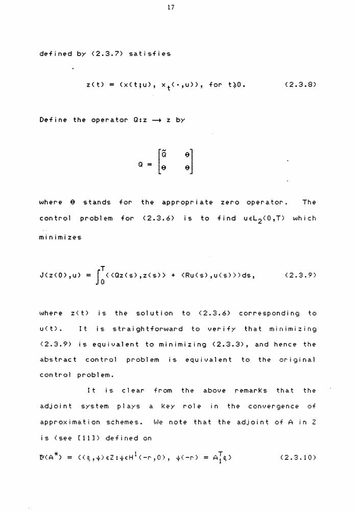
defined by <2.3.7) satisfies

z < t) = < x < t ; u) , x t < • , u) ) , for t ~o . (2.3.8)

Define the operator Q:z-+ z by

Q = [! :] where e stands for the appropriate zero opera tor. The

control problem for <2.3.6) is to find uirL2 <0,T) which

minimizes

T J ( z ( 0) , u) = r < < Qz < s) , z < s) > + <Ru< s) , u ( s) >) ds,

• 0 (2.:=:.9)

u (t) • It i:. -:.traightforwar·d to verify that minimizing

(2.3.9) is equivalent to minimizing <2.3.3), and hence the

ab:.tract control prc•blem is equi•.•alent to the or·i•;;:iinal

contr·ol problem.

It i :. c 1 ear from the above remarK:. that the

adjoint system plays a Key role in the convergence of

approximation schemes. l,..Je note th.:i.t the adjoint •:•f A in Z

is Csee [11J) defined on

(2.3.10)

18

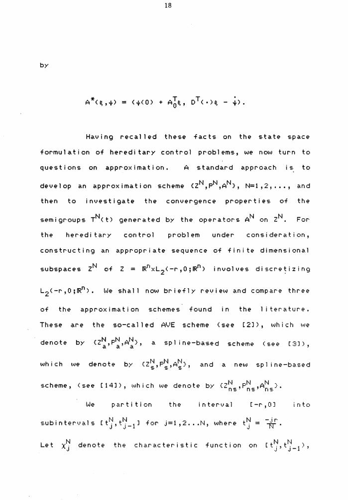
by

* A <~,.p = T T . <+<O> + A0 ~, D <·>~ - +>.

Having recal 1 ed these facts on the state :.pace

formulation of hereditary control problems, we now turn to

questions on approximation. A standard approach is to

develop an approximation scheme <ZN,PN,AN}, N=l,2, ... , and

then to investigate the convergence properties of the

semigroups TN(t) generated by the operators AN on zN. For

the her·edi tary problem under consider-ation,

constructing an appropriate sequence of finite dimensional

subspaces of z = involves di-:.cre~izing

L~<-r,O;~n). We shall now briefly review and compare three ~

of the appr-oximation schemes found in the literature.

These are the so-called A\.-'E scheme (see [2J), \.oJhid1 •.A.It?

denote b>' a spline-based scheme (see (:3)),

scheme, (st?e [14J), which we denote bv f7N pN AN 1 ' -~n:.' n:.' n:.··

We the interval [-r,OJ

N N subintervals [tj,tj-l] for j=l,2 ... N, where N - .. i r· t . = .J 1T .

Let • )'-1 .A: j denote the char·ac ter i st i c

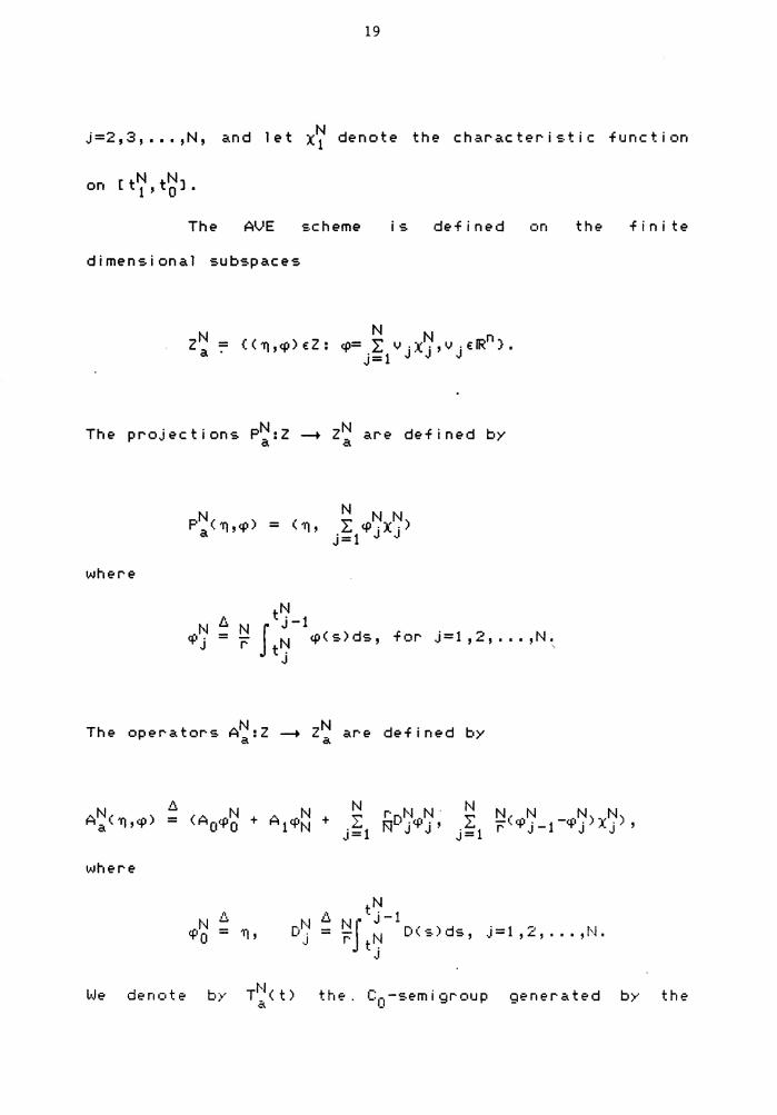
19

j=2,3, ••• ,N, and let X~ denote the character-is.tic function

N N on rt 1 , t 0 l •

The A'v1E s.cheme is defined c•n

dimensional subspaces

The projections P~:Z-+ Z~ are defined by

where

tN j-1

N N N I: <P·X·) j=t J J

J N <P(S)ds, tj

for j=t ,2, ••. ,N. '

The operators A~:Z-+ Z~ are defined by

where

D. tt':J

the

,,,,N = ...... ' "'0 ., cl:1 .J

b. NJ. J -1 , = r N D~·:.)ds, j = 1 ' 2 ' • • • ' t--l • t. ,I

~·Je denc•te bv the. c0 -semigroup generated

finite

the

20

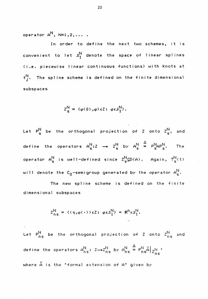
oper·a tor AN, N=1,2, •••

In order to define the next two s;.chemes, it is

convenient to 1 e t N .,3,:1 denote the space of 1 i near sp 1 i nes

( i • e. pi ecew i s;.e 1 i near continuous functions) ~"' i th Knc•ts:. at

t~. The spline scheme is defined on the finite dimensional J

subspaces

Let be the orthogonal projection of z onto and

define the operators = The

opera tor A~ is well-defined since z~s;D<A). Again,

will denote the c0-semigroup generated by the operator A~.

The ne•>J spline scheme is defined C•n the finite

dimensional subspaces

= JRnx fl..N . -" 1 •

Let the C•f z a.nd

define the c•pera tors:. AN · 7-+ ,H n s. • ._ '- n -:.

~

where A is the "formal extension of A" given by

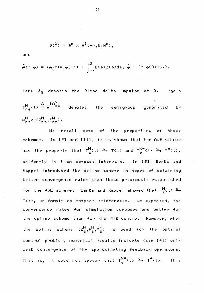
21

and

Here 6 0 denotes the Dirac delta impulse at 0. Again

denotes the semi group generated by

AN ~L<ZN -,.N ) ns- ns''"n:. •

We recall :.ome of the properties of the-:.e

schemes. In [ 2) and [11 J ' i t i <,;;. shown that the Al..-1E :.cheme

ha:. the property that TN(t) a

s ....;;....+ T<t) and Tt·-.I* < t) a -4 T*. t. •:. ) '

•Jniforml>' in t C•n compact interval-: .• In [3J·, BanKs and

Kappel introduced the :.pl ine scheme in hope:. of obtaining

better convergence rates than those previously established

for the AVE scheme.

T ( t) , u n i form 1 y on c c•mp act t - i n t er· v a 1 -:; .• A:. expected, the

convergence rate-:. for s i mu 1 at i •:•n purpose:. ar·e better fc•r

the sp l i ne -:.cheme than fc•r the Al,,JE :.cheme.

is •J<.:.ed for the optim.:i.1

contr·ol pr·oblem, nwner·ic-".l r·es.ult:. indic.:..te (s.ee [4]) onl;.-·

wea~~ •:on\.>ergence c•f the ~.ppr·c·ximating feedba·=~~ oper·atc•rs.

That i ·=·' it does. not appe.:i.r· Thi:.

22

result is not surprising, since A~~A* and the spline scheme

N . N * has the proper b' that ZsC8(A) v.Jh 1 1 e Zs 't8<A ) ( r·eca 11 Remark

2.2.2). Although the numerical evidence indicates that

T~* < t) does not converge strongly to T* < t), it has. not yet

been established that this is in fact true. This

interesting question remains unanswered.

One attempt tc• resolve this. i:iroblem is to relax

the definition of the finite di mens. i ona 1 subs.paces zN so

that zN contains "sufficiently many" elements of both 8CA>

and 8<A*>. The new spline subspaces Z~ have this property,

and the new spline scheme {7N PN ANl does satisfy (2.2.5) -ns' s' s·

and <2.2.6) <see [14]),

Remark 2. 3. 1 In general, when one defines an approximation

s.cheme with zNC8(A), then the operators AN can be defined

Further·mc•re, if A is dissipative, then it

follows immediately that each AN is. di-s.-s.ipative, a.nd hence

the stability cc•ndition Hl) of The•:•rem 2.1.1 ·is. eas.ib'

verified. However, if A~~A*, then zN may not be a subspace

of B\A*> .:c.nd the -s.cheme m.:c.y nc•t 1 ea.d tc• an apprc•x i mat ion

(i.e. in the -:.tr·c•ng c•perator· topology) of the .:c.d . .ioint

semi gr·c••Jp. If one attempts to avoid this problem bv

23

defining an approximation scheme with zN¢r:J<A), then PNAF.N

is not well-defined, and one is presented with the problem

of defining the operators AN appropriately <the AVE scheme

fa l l :. i n to th i s cat e gc•r y) . In addition, it i:. no lc•nger

trivial to tJerify the stabilit>· condition H2) of Thec•rem

2.1.1. In the next section, we develop a general framework

for the problem of defining the o~erators AN so that even

in the non self-adjoint case, conditions <2.2.5) and

(2.2.6) hold.

24

2. 4 6. genera 1 framewc•rk fc•r approximation

As mentioned in the closing remark of the

previous section, we shall now present some results in the

direction of a general framework for construe ting

satisfactory approximation :.chemes for the 1 i near, quadratic

cost optimal control problem.

Let A be the infinitesimal generator of a.

c0 -semigroup T<t) on a Hilbert space z. The problem is to

define an approximation scheme {ZN '

pN ' AN) which

satisfies

i) PN ~I

i i) TN< t )~T< t), uniformly in •:ompac t

t-interuals

iii) TN*<t)~T*<t), uniformly in compact

t-intervals,

where TN(t) = etAN

A:. indicated abo~.ie, if A=:tA*, then an appropriate .:i.pproa.ch

to this problem is to choose approximating subspaces

N Z C I.HA). If AN D,

i :. defined by AN = PNAPN, then under

. t b 1 d. t . 7N d pN d. t . ''"' 2 c' . 1 1 SU I a e con I I on=· C•n - an ' c C•n I I C•n ~ /:. • • :.:.• J IJ.J I

i mp 1 >' < 2 • 2 • 6) • l"lhen A::t:tA*, then (a:. i :. :.een f•:ir· thE-

her·editary contr·ol pr·ob1€'m) it is possible that zN •+ 1-HA*)

and (2.2.6) may not hold. Our approa.ch i :. to define the

25

approximating subspaces so that "contains

sufficiently many elements" of both B<A> and B<A*>.

However, in this case t>'P i ca 11 y zN¢B<A>, so that PNAPN i -:;.

no 1 onger we 11-def i ned, and cannot be used to define AN.

Therefore, we will construct a bilinear form cr which

extends A and A* in an appropriate manner, and define AN by

restricting cr to the subspaces zN. We discuss a technique

for constructing the bilinear form a. Ass•Jme that V is a real Hilbert space with the

trace property (see [ 17]); that is,

v c z=z* c v*

and there exists y € L<V,H) so that

Here, H is a Hilbert space and Z is a pivot space

([1l,C17J) and is identified with its dual z*. Assume also

that Ker y = v 0 , and the inclusions VCZ, v0cz are dense and

continuous. That is, there are c 1 , c 2 >o sc• that

llxll 2 ~ c 1 11xllv

PROPOSITION 2. 4. 1 In the above framework, 1 et A be a

closed, dense 1 >'-defined 1 i near op er.;.. tor in z with

B(A) = v0 ~ V. Assume that B<A*>CV and there is a constant

K such that llA*u11 2 .~ t-::llull~) fc•r· all ui!I'f(A*>. If there i -:. an

26

operator ae:L<'v1 ,Z) which extends A <i.e. alv =A), then 0

there exi-:.t-:. * 6e:L<V,H ) so that the bilinear form a on VxV

given by

A cr<u,v) = <au,v> 2 + (yu,6v>H

is bounded and has the property that

i) cr<u,v) = <Au,v>z for all ue:B<A>, ve:V,

and

ii) cr<u,v) = <u,A*v>z for all ue:V, ve:B<A*).

Proof: Since Q.;:L<V,Z), it fol lo~"'=· that there i-:. ~. consta.nt

K1 such that for all u e: V

A * <Cu>Cv) = <v,A u> 2 - <av,u> 2 .

Then C is bounded since

-=·up I I I I llCull * .~ ve:• .. ...i { <i.,• ,A*1J>z + <av ,u> 2 } 'v1 llvllv=l

* {: c llA IJ 11 2 + 11a1) 11 2 ·llu11 2

Note that ye:LCV,H) i '=· on t C• , * * * and hence y· E LCH·,v > i-:. 1-1,

Observe that since [Ker y]l is

27

a Hilbert space with norm 11·11 *' l) .

* then 'Y is a continuous

1 inear bijective c•perator from H* onto [Ker 't)l. Hence,

<see Theorem 4.3.3 in C1J),

define ion 8<A*> into H* by

,..., * -1 ov = ("}"· . ) Cv.

Note that this is •Ale 11 -defined since 'R<C>=CKer •}""] l = ~

Also, o· is bounded since and C are ....,

bounded. Let o be the extension of o to a bounded operator

on all of V, and define the bilinear form a on VxV by

J}, a<u,v) = <au,v>z + <Tu,&v>H.

Property i) is clearly satisfied. To e-=:.tabli-=:.h ii),

observe that if •.J E:8(A *>, then

= = ( Cv) ( •J) for al 1 The

re-:.u l t fol l C•t.• . .r: ..

28

Although the previous res~lt provides only the existence of

6, we have the following partial characterization of 6.

LEMMA 2. 4. 2 If o£L(lv',H*) is as in Proposition 2.4.1, then

Pr•::1of. Note that ACQ implies 8<a*)C8<A*). If

then v£8<A*) and for all U£V 1..ve have tha. t

Therefore, 6v:o. On the other hand, if v i::tHA *)(ll<er 6 a.nd

u£V, then

O=cr<u,v)-<u,A*v> 2 =

and hence v£8<a*>.

* <au,v>z - <u,A v> 2 ,

ii

We apply these ideas in practice by investigating

!HA*) and D'<Q*) to determine.:::, and hence·~. kle then

choose appropriate approximating subspaces zNcv, and define

the operators AN by restricting cr to zN. That i-:., define

/ . .,N ' 'H U, \) .. · z ~ = cr ( u , •.) ) j .,N . '-

l;Je then s.h 1:;11,0.! of the re·:.ulting

approximation scheme. Let us consider an example.

29

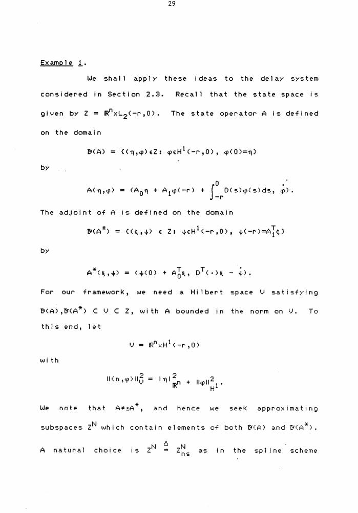
Ex amp 1 e l·

We shall apply these ideas to the delay :.y:.tem

considered in Section 2.3. Recall that the state space i:.

The state operator A is defined

on the domain

by

Io . A<~,o:p) = <A 0 ~ + A 1-:p<-r> + D<s>~<s>ds, ~).

-r

The adjoint of A is defined on the domain

by

For our framework, we need a Hi 1 ber t :.pace V sat i ·:.f;.' i n9

DCA), D<A*> C V C Z, with A bounded in the norm on V. To

thi:. end, let

with

We note that

~.

ll(n,o:p)llv = ., llq:tll .... 1 •

H

and hence ·:.e eK approx i ma.ti n•;i

b ~N i... i.. :.u :.pa.ce:. L 1J.J11 1 c11 contain elements of both DCA>

A natur·.:..l choice i -=· = in the sp 1 i ne scheme

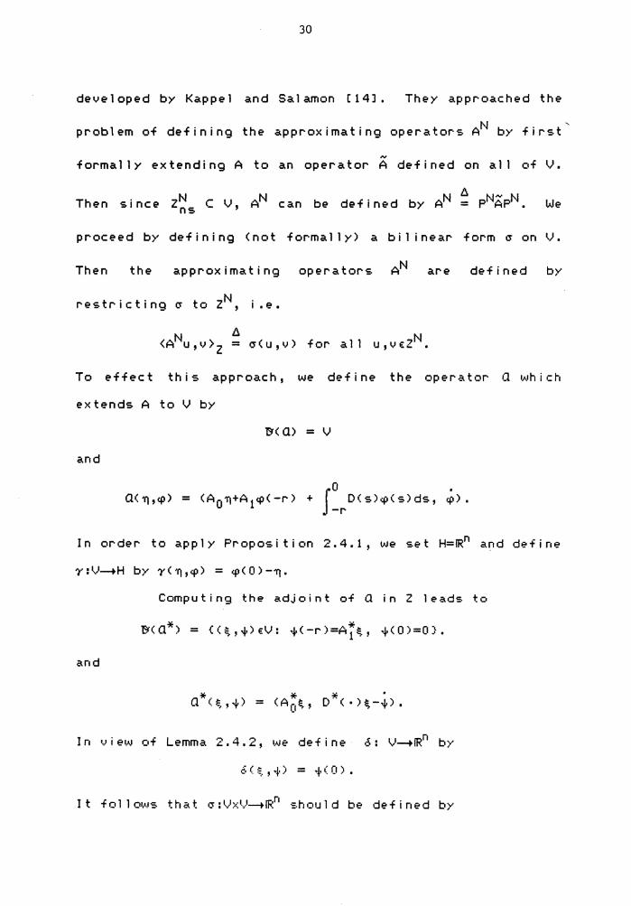
30

developed by Kappel and Salamon [14J. They approached the

problem of defining the approximating operators AN by first

~

formally extending A to an operator A defined on all of V.

Then s i nee Z~s C V, AN can be defined by AN ~ PNAPN We

proceed by defining <not formally) a bilinear form cr on V.

Then the approximating operators AN are defined by

restricting cr to zN, i.e.

N ~ N <A u,v>z = cr<u,v) for all u,v€Z .

To effect this approach, we define the opera tor (1 1.._1h i ch

extends A to V by

~(Q) = v and

In order to apply Proposition 2.4.1, we set H=IRn and define

Computing the adjoint of Q in Z leads to

and

In •,ii e•,\I C•f Lemma 2. 4. 2, •Ale define .5: V-+IRn bv

6(:~_,.p = ·i·((I),

It follov . .1s that cr:~h:'·....f-+~t· :.hi::i•Jld be defined by

31

We ar-e now in a position to define an appr-ox i mat ion :.cheme

N=1,2, ••• , with Define the

tJ. approximating subspaces. zN by zN = z 1~s <see Sect i c•n 2. 3)

and 1 et pN be th th 1 . t· f 7 0'"'1t._-, zN. e or ogona proJec ton o - ,

use a to define AN: ZN-+ZN by

for a 11

A direct calculation verifies that

for a 11 N •J ,vE:Z • Therefore, ~'•hen the above frame1,•,1or·K i ·:.

used to develop a spline-based approximation scheme for the

hereditary contr•::il problem, it leads to a scheme (in thi:.

the new spline scheme

satisfies (2.2.5) and <2.2.6).

Chapter III

PARTIAL FUNCTIONAL·DIFFERENTIAL EQUATIONS

3.1 State Space Formulation

In this section, we consider the problem of

developing a state space formulation for a PFDE of

hyperbolic t>·pe. Well-posedness will be obtained by

showing that the underlying operator is the infinitesimal

generator of a c0 -semigroup. First 1,<Je briefly di-:.cu:.s

·:.evera 1 recent and re 1 evan t pap~:"~ ( -:.ee [SJ, [ $'), [ 16J,

[22J' [23J). In many of these investigations, the PFDE is

treated as .:.,n initial value problem for an abstract

ordinary functional differential equation of the form

0 u(t) = A 0 u<t) + A 1u(t-r·) + J a(s)A...,•J(t+s)d:. + f(t) <3.1.1)

-r ...

u(O)=~, u(s)=·ri<:.) a.e. in [-r,OJ (3.1.2)

where A0 :&<A0 )CH-+H i =· the infinite:. i ma 1 genera tc•r· •:if an

analytic semi group in a Hilbert space Hand A1 ,A2 €LCDA- ,H). '-'

Here,

In order to use semigroup techniques, i t i =· ar·gued that (3.1.1)-(3.1.2) i·:. t.oJell-po:.ed vJith initi.:..l d~.t.:..

fr· om :.ome sp .:<.c e Z = >< x L--:. ( -r , 0 ; '() • ... A solution semigroup

T<t> i:. then defined on Z .:..nd the infinitesimal gener .. ;.tor A

32

33

of T<t> is characterized. This appr·oach is u-:.ed in [9J tc•

-:.tud>' the stability of (3.1.1)-(3.1.2) via the spectr-al

properties of A.

An important problem in this approach is the

prescription of appropriate in i ti a 1 data that

< 3. 1 • 1 ) - < 3. 1 • 2) i s •.Ne 1 1 -posed. Kuni sch and Scha.ppacher·

have shown in [16J that if one makes the natural assumption

tha:t <~,'l'f) E: H x L 2 <-r,O;H), then <3.1.1)-(~:.1.2) i-:.

generally not well-posed; It has been -:.ho1.·m that the

appropriate choice for initial data is

where F is a suitable interpolation space between DA and H 0

<see t7J and [8]).

However, when considering PFDEs of hyperbolic

t>'pe, one does not have recour·:.e to these •.Ne 11-po-:.edne-:.s

results for- the corresponding abstract FDE. Thi·:. i-:.

becau-:.e in the hyperbolic case the oper·.:c.tor A 0 in the

cor·res.ponding abstr·act F.DE typically i-:. nc•t the gener·atc•r·

of an ana 1 yt i c semi group. Since we wish to use semigroup

techniques for approximation and control of hyperbolic

PFDEs, we will use a different approach than that mentioned

Th.£\ t i :. , •.-<Je do not •Js.e the t.<_1e 11 -pc•-:.i?dnes.·:. of the

abstrc..ct FDE to define .£\ :.olution semigr·c•up. P.:c. th er, 1_.,_1e

conjecture an equivalent <E.tate space for·mulation c•f the

form

z = Az<O + F<t)

z((I) = z 0

on a state space Z. The opera tor A i =· construe ted u<E. i ng

the dynam i C'E· C•f the PFDE. The above-mentioned results of

K•Jnisch and Schappacher [16J indicate that v..1e m•J<E.t m.:..ke a

judiciou<E. choice of the state =·pace in order that the

problem be r,._1e 1 l -posed. Recall that the above problem i<E.

well-posed if and only if A is the infinitesimal generator

of a c0 -semigroup on z.

With this in mind, we consider the following

hyperbolic PFDE which arises in viscoelasticity:

J.o .~2 + g(s)~\; z~·'<t+s,x)d<E.

-r .:i )< (~:.1.~:)

yCt,a) = 0 = y(t,b) (3.1.4)

y ( 0, x) = s ( x) , iT_y ( 0 , ::<) = v ( x) for· a{'. x .~; b (3.1.5)

y(t,x) = hCt,x> for (3.1.6)

continuous function g0 :R-~R- satisfying

35

g 0 <s><O for -r<s~O

g 0 <s>=O for s~-r

and such that:

i )

i i )

i i i )

g<s>~g0 <s> for -r<s~O

€ 0 ~€, where € is defined by

0 € ~ ~ + J g(s)ds

-r

The existence of € 0 fol 1 ows from genera 1 properties of

e 1 as t i c mo du 1 i • Condition iii) is a "decaying memor>·"

assumption. For a further discussion of the physical basis

for these assumptions, see C13J and C24J.

Throughout the rest of this chapter, •.AJe shall

often use the symbol to denote differentiation with

respect to the x variable. We now pose the above

viscoelastic problem in the state space

(3.1.7)

with norm defined by

36

The operator A is defined on the domain

by

(3.1.8)

Note that A has the form

A(!) Ao(:) Jo to• + G<:.)Anl Id~ = -r - w -'

dt.<J dS

r,,,rhere

(~ ((

i<l Ao ( ~) (~ ~~;) p

('~:) = = 0

.:i.nd

,' 1 0) . G(s) = l-Q ( <=.) c.-.:- . -0 o,

We :.hall establi:.h that A gener.:i.te: .. :i, c0 -:.emigrc••Jp c•n Z.

Hm-11ever·, it i"' import.:i.nt to note that there ar·e ma.n;•'

pos-:.i bl e st.:i.tt? -:.pace formu 1 at ion-:. of the :. > .. -;. t Er rn

(3.1 .3)-(3.1 .6). l.Jal ker· [24J •:on:.tru•:ted .:i, di ffer·t?nt :.ta.ti?

:.p.:i.ce model and u·:.ed hi:. model for~. -:.tattility an.:i.1;.-·:.is.

We shall makt? use of Walker's results; thus it i =·

37

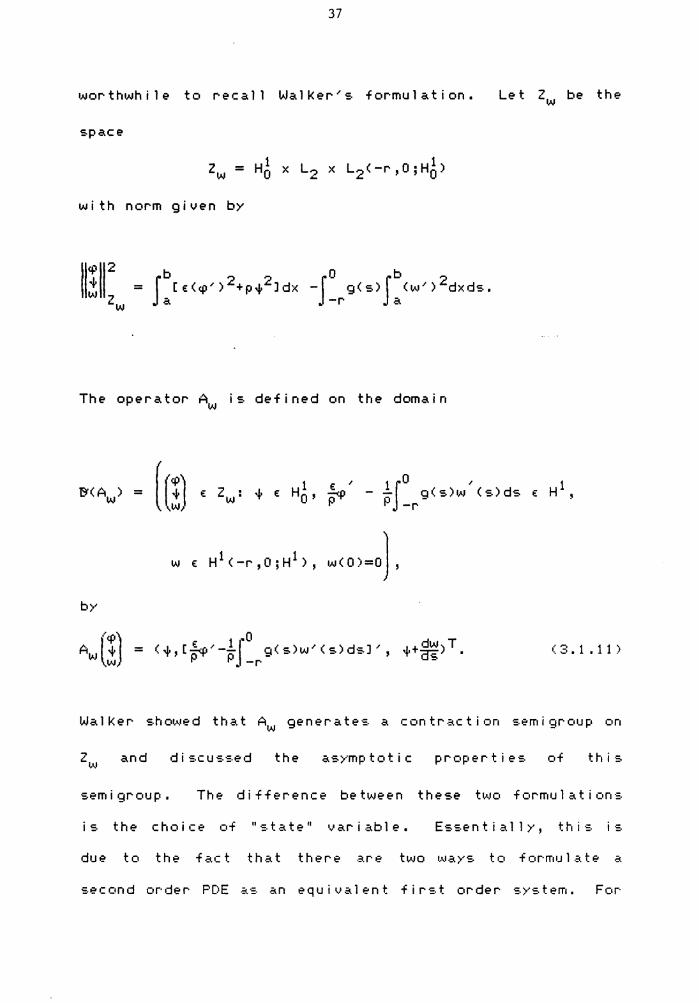
•JJor t hwh i l e to recall Walker's formulation. Let

space

with norm given by

11111: = w

The opera tor Aw i =· defined on the domain

(m 1 ~ ,

- ·~J~r g( s)1,..,' < s) ds '&<Aw) = E: Zw: i· E: Ho' p

w E: H1 <-r,O;H1), w( 0 )=0) , bv

(~) A~,l~ = ~ 1 ro ( ·h [tf'' -P. -r g< s)w' ( s) ds]', i·+dw) T as

E:

Z be the w

H1 '

(3.1.11)

Wal Ker showed that Aw generate·:. a cc•n tract i •:in :.em i grc•up on

z~\I and discu:.:.ed the asymptotic prc•per tie:. c•f th i ·s.

semi grc•up. The difference between these two formulations

i:. the choi•:e of ":.t.ate" variable. Es:.enti.ally, thi:. i·:.

due to the fact that there .:i.re two •A•ays to for·m•Jl .ate ~.

second order PDE as an equivalent first order system. For

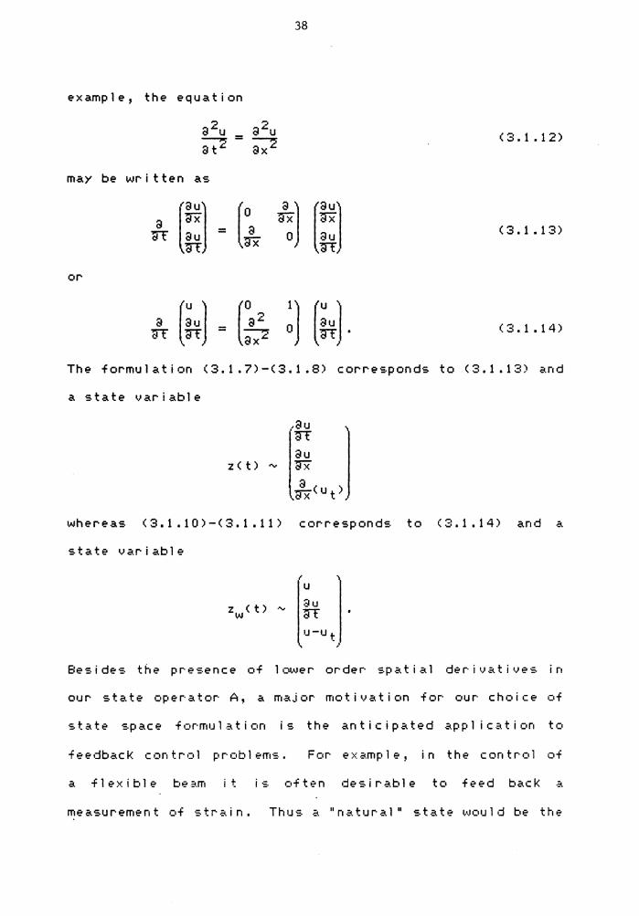
38

example, the equation

(3.1.12)

may be written as

a (~) = ( 0

~ ~ b: (3.1.13)

or

(3.1.14)

The formulation <3.1.7)-(3.1.8) corresponds to (3.1.13) and

a state variable

z ( t) ,...,

whereas ( 3. 1 • 10 )-( 3. 1 • 11) corresponds to ( 3. 1 • 14) and a

state variable

Besides the presence of 1 ower order· spat i a 1 derivatives in

our state operator A, a major motivation for our choice of

state space for·m•.Jlation is the anticipated appl icatic•n tc•

feedbacK control problems. Fc•r example, in the control of

a flexible beam it is. often desirable tc• feed back a

measurement of strain. Thus a "natural" state would be the

39

strain When one applies our state space formulation

to the problem of control 1 i ng a f 1 ex i bl e beam, the strain

is part of the state, which is riot the case for other

for mu 1 at i on s • Besides this feature, another advantage of

the formulation <3.1. 7)-(3.1 .9) is that the operator and

state space structure is ana 1 ogous to that for ordinary

func ti ona 1 differential equations. Indeed, after

discretizing the spatial variable in <3.1.7)-(3.1.9), v .. •e

are 1 ed to a fam i 1 i ar FOE opera tor. This will be •J~.eful

for approximation.

In the remainder of this section, we address the

question of well-posedness of our state space fc~mulation.

That is, we show that A is the infinitesimal generator of a

c0 -semigroup. We w i 11 malt~e reference to some resu 1 ts in

C8J, where a state space formulation is developed for a

PFDE of para.bol i c h'pe. DiBlasio, Kunisch and Sinestrari

shov.ied that the underl>'ing operator· is the infinite~.imal

generator of a c0-semi group. l..<Je will use this fa.ct to

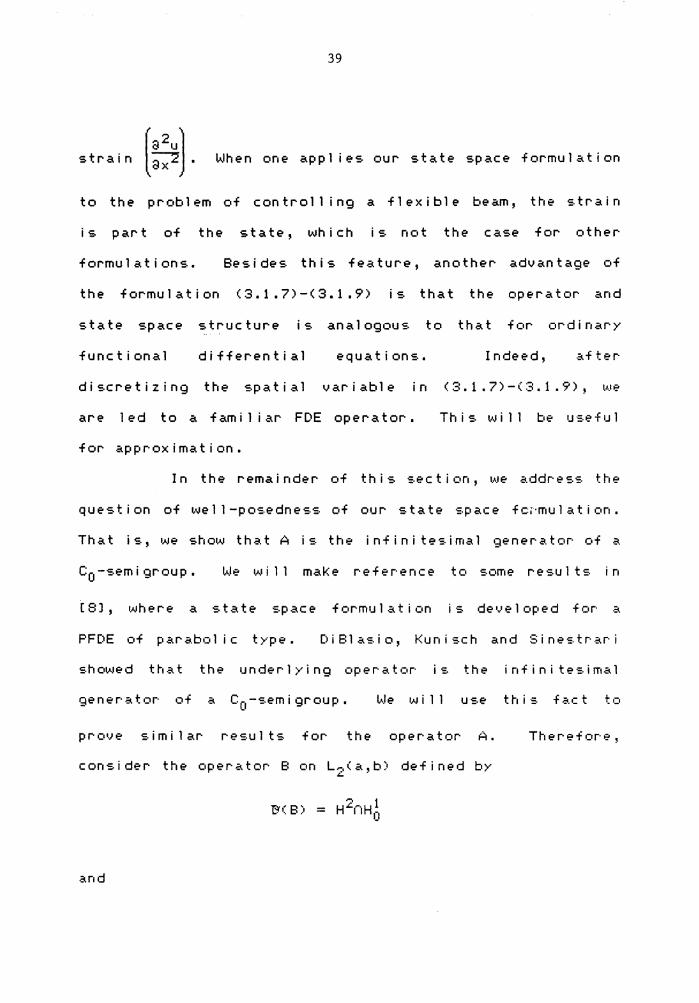
prove similar results for the operator A. Therefor·e,

consider the operator Bon L 2 <a,b) defined by

l'j( 8)

and

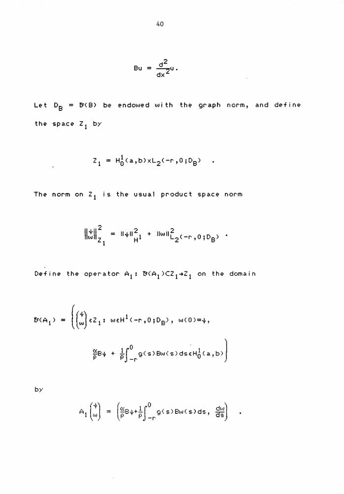
40

d2 Bu = -u. dx""

Let 0 8 = B< 8) be endowed with the graph r1orm, and define

the space zl by

2 1 = H6<a,b)xL2 <-r,O;D8 )

The norm on 2 1 is the usual product space norm

11 1·11 2 = 111.11 2 1 + llwllt (-r,O;D8 ) . w 2 H 2 1

Define the operator A1 : BCA 1 >cz 1 ~z 1 on the domain

l:~<A 1)

b>··

( ( ·r) = lw,1i::Z1: wi::H 1 <-r,O;D8 >, wCO>=+,

~B·r + -bl.o g(s)8w(slds<H6<a,bl 1 P • -r· ,.

Al (.~) = •' n 'J c·· 1 • - . di,•J l ....:.s.~.+-j Q ( :.) Bw< =· > d:., os. p p -r- -'• .

41

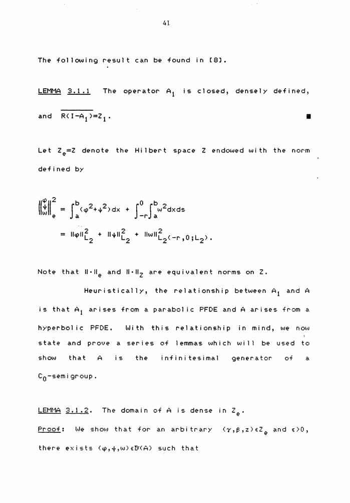
The following result can be found in C8J.

LEMMA 3. 1. 1 The operator A 1 is closed, densely defined,

• Let Ze=Z denote the Hi 1 bert :.pace Z endowed with the nor·m

defined by

2 .... 2 = llcpllL + ll;,11..:.L + llwllL <-,.., o. L )

2 2 2 I J ' 2' '

Note that ll·lle and ll·llz are equivalent norms on Z.

Heur i st i cal 1 y, the rel at ions.hip betv.Jeen A 1 a.nd A

is that A 1 arises from a parabolic PFDE and A arises from a

hyperbcil i c PFDE. W i th th i s re 1 at i on sh i p in mi n d, we n or.AJ

state and prove a :.er i es of 1 emmas which '-<Ji 11 be us.ed to

show that A is the infinitesimal

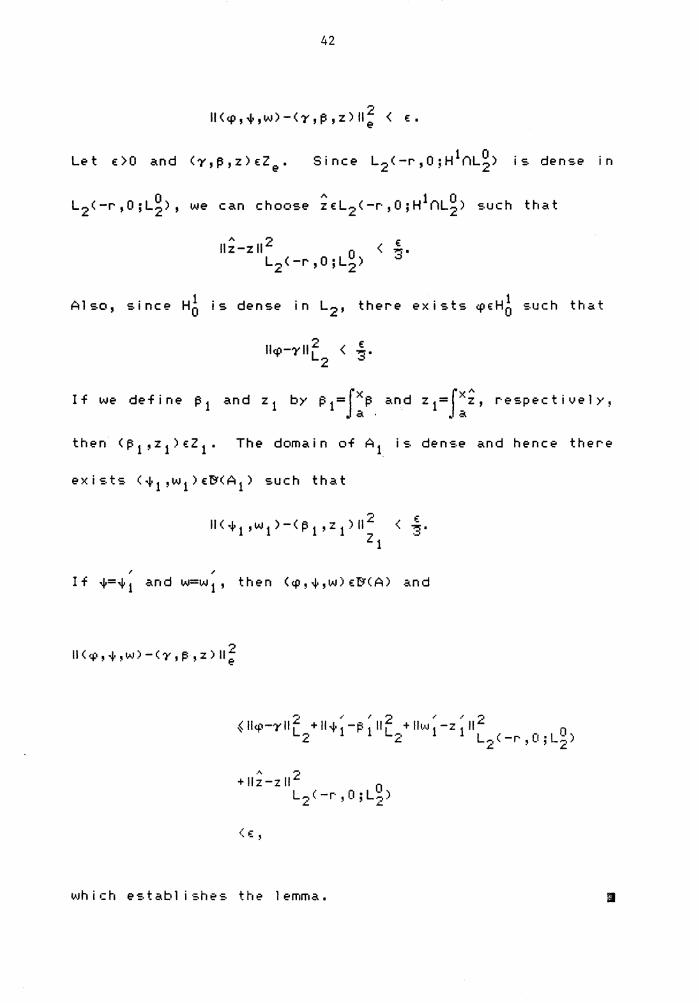
LEMMA 3.1.2. The domain of A is dense in 7 '- e •

Pr·oof: We show that for an arbitrary

42

2 ll<cp,+,w>-<'Y,f~,z)lle < €.

Let €)0 and (-y,13,z)€Ze. Si nee L2 <-r, 0; H1nLg> is dense in

L2 <-r,O;Lg), we can choose ;€L2 <-r,O;H1nLg) such that

A 2 € llz-zll 0 < ~·

L2 <-r,O;L2 )

Also, since HA is dense in L2 , there exists cp€HA such that

2 € llcp--y II L < ~ • 2

If we define 13 1 and z 1 by 13 1=J:l3. and z 1 =J:~' respectively,

then <13 1 ,z 1>€Z 1 • The domain of A1 is dense and hence there

exists <+ 1 ,w 1 )€B<A 1> such that

ll<-+1,w1>-<131,z1>112 < ~· 21

, , If +=+ 1 and w=w 1 , then Ccp,+,w>€BCA) and

2 ll<q:i,-f,w>-<-y,13 ,z) lie

,,. ,, 2 ,,. .~ 2 ~ llcp--yllC + ll+1-l31 11 L-.+ llw1-z1 11 L .. ,<-r, O; L~)

2 ~ ~ ~

... 11 2 0 +llz-z L,...,(-r·,O;L2>

~

< € '

which establishes the lemma. •

43

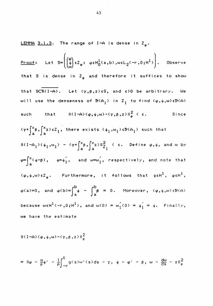
LEMMA 3.1.3. The r-ange of I-A is dense in Ze.

Pr-oof: Let s=( (!)a.: ~·HA<a,bl,w<L2<-r,o;H 1 l). Ob:.er-•Je

that S i :. dense in Ze and ther-efor-e it :.uff ices to :.ho1J..•

that SC'R< I -A) • Let (')',13,z)E:S, and E:)O be ar-bitr·ar-y. l..Je

vJill use the densene:.s of B<A 1 ) in z1 to find <q:•,1-,w)E:D"(A)

:.uch that ll<I-A)«p,·¥,w>-<1·,13,z)ll; < E:.

(7+Jx13,Jxz)E:Z 1 , ther-e exists <+ 1 ,w 1 >E:B<A 1 ) such that a a

s i rice

ll<I-A1)<t1,'·"'1) - (7+fx13,Jxz)ll~ < E:. Define cp,+, and w by a a 1

, , q:i=Jx<+-13),

a ·¥=+ 1 ' and w=w 1 , r- e :.p e c t i \} e 1 y , and n c• t e that

(cp,.¥,w) E:Ze. Fur-ther-mc•r-e, it fol 1 ows that i·E:H 1 , q:•E:H 1 ,

b b cp( a)=O, and q:i< b)=J + - J ~ = 0 •

a a Mor-eo1.ier, (.:p,.i0 ,1J..1) i::I'1"(A)

because wE:H 1c-r-,O;H 1 >, and w<O> = , ,

tJJ1 (0) = +1 = ·¥· Fir.all)'··,

we have the estimate

II ( I -A) C:p , + , w) - C 7 , ~; , z ) II~

Ci! ·" = llq:i - p-+ 0 lf g(s)w'(s)ds - y, + - cp'

P.-r dw - i::, tJJ - as z 11 2

e

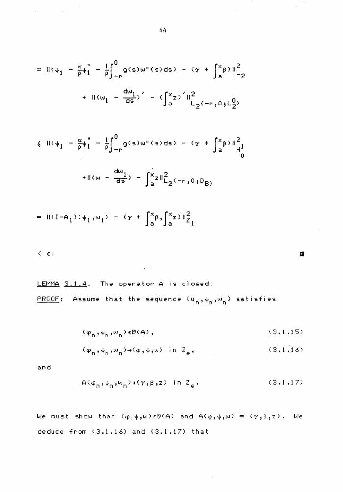
44

< e: •

LEMMA 3.1.4. The operator A is closed.

PROOF: Assume that the sequence Cun,+n,wn> satisfies

(3.1.15)

«+· • ·~ ,w )-+(.;p' t ,r,v) in ze' n · n · n · (:3.1.1.!1)

and

A(1.p , ·i· ,v . .r )-+<"t', 13, z) in Z~_-. n · n n · · ~ (3.1.17)

We must show that (~,+,w>e:B(A) and A<~,+,w> = <~,13,z>. We

deduce fr·eirn (:3.1.10:::.) .:..nd (3.1.17) that

and

wie:H 1<-r-,O;Lg)

dw _ as - z •

45

(3.1.18)

(3.1.19)

This imp 1 i es that Wn-+W in H1 <-r-,O;Lg> and +n = wn(0)-+w<O>

. LO I n ? • ""

However-, (3.1.15) implies that +n-++ 0 in L2, and

hence

w< 0 >=+.

Simi 1 ar- 1 y, ( 3. 1 • 1 6) imp 1 i es that

0 0 ~+n + tf _r-g(s)wn(s)ds-+ ~++tf _r-g<s>w<s>ds

and (3.1.17) yields

C< / t Jo / p'fn + P -r-g(s)wn<s>ds-+ 13 in L2 •

Consequently, we conclude that

0 ~+ + .!.J g( s)t1,1( s) dse:H 1 p p -r-

and

c ~~. + lf 0 c:i< s)•,<J( s) dsJ / = p P. -r·- 13 •

0 in L2

( 3. 1 • 20)

(3.1.21)

(3.1.22)

46

Again, a similar argument yields

( 3. 1 • 23)

and

<P'=-y • (3.1.24)

The identities, (3.1 .16), <3.1 .17) and (3.1 .24) together

imply that <Pn~<P in H1 , which implies that

<P<a>=O=<P<b>. ( 3. 1 • 25)

Combining (3.1.18), ( 3. 1 • 20) ' (3.1.21), (3.1 .23), and

A 1 so < 3. 1 • 1 '?' > ,

( 3. 1 • 22) and ( 3. 1 • 24) imply that

Therefore, A is closed. • We note that A does not satisfy a dis~.ipative

type of inequality on z. We introduce a dissipative ,..,

operator- A which is simi 1 ar to A, and use the ,..,

dissipativeness of A and its similarity to A to facilitate

proving some of the fol 1 owing resu 1 ts, inc 1 ud i ng thc•se C•n

approximation in Section 3.2.

With this in mind, define the operator· L1;:L<Z,Z>

by

= (~ ) . i--w,

47

'Note that L- 1=L, and Lis bijective. We sha 11 need the

following results.

LEMMA 3.1.5 Let H be a Hilbert space and let LE:L<H,H) be a

bijective operator satisfying L=L- 1 • Suppose 8 is a

closed, densely defined operator in H and 'R(~l-8) = H. If ,..,.

the operator 8 is defined on the domain ,.,

&<8) = {xE:H: LxE:&(8)}

,..,. ~ 1 ,..,. ,..,. by 8 = L- BL= LBL, then B is closed and 'R<wl-8) = H.

,., ,..,.

Proof: To show that 8 is closed, assume that xnE:IHB>,

,..,. n=1 ,2, •.• , and xn -+ x and Bxn -+ y. It follows that

Lxn E:&( B>, n=1, 2, ••• , and Lxn -+ Lx and BLxn -+ Ly.

Therefore, since 8 is closed, LxE:9(8) and BLx =Ly. Hence, ,..,. ,..,. ,..,.

XE:&(B) and Bx = y, which proves that 8 is closed.

N

To show that 'R(wl-B> = H, let xE:H and €)0 be

arbitrary. Si nee 'R<wl-8) = H, there exists >'E:°&(8) such

that ll<wI-8)y - LxllH < rr0r· ,..,. Consequently LyE:9(8), and

,., ll<wI-B)Ly - xii = llL((.:il-8)y - LLxll

~ llLll•ll(t.:il-8)>' - Lxll < € •

48

LEMMA 3 .1. 6 Assume that the hypotheses of the pre\J i ous ,....

lemma hold. If 8-l is dissipative for some l<w, then B is

the infinitesimal generator of a c0 -semigroup S<t)

satisfying llS(t)ll ~ llLll 2ewt.

Proof: If B-). is dissipative, then <wI-B)-l is a closed,

bounded operator, and i t follows that ,....

Therefore, '&( B> is dense <see [18J). Hence by the

"' Lumer~Phill ips Theorem B is the infinitesimal generator of

Therefore,

L- 1§<t>L is also a c0 -semigroup, which we denote by S<t>.

shows that

1 i m S( t) z-z t l 0 t

L- 1BLz = B.

Thus, 8 is the infinitesimal generator of S<t>, and the

re :.u 1 t f o 1 1 ows •

In order to app 1 y the:.e resu 1 ts t•::i our problem, we define

.~·

the operator A on

49

= ((!)€2: cp€H6, i€H 1 , w..:H 1<-r,O;H 1>,w<O>=o),

by A~ L-1AL. In particular, it follows that

,.., (<P) , 1 Jo , ' ' dw A+ = <~i -- g(s)w <s>ds,q> ,<P -crs>· . w P P -r

,.., We now show that A is di ss i pat i ve and hence generates a

c0 -semigroup of contractions.

,.., LEMMA 3. 1 • 7. The operator A generates a c0 -semi group on

2.

Proof: If (!)€°&(A), then

2<A (~) , (!) >2

f b Jo . Jb =2 [€+' - gCs)w'(s)dsJcpdx + 2 E:<P'+dx a -r a

- 2J0 g< s>Jb [q/ + ~Jwdxds -r a

0 b = -2J g( ~.)J VJ~d~<d·:.

-r a ·

50

Io d Jb 2 ~ osg(s) w (s)dxds -r a

0 b ~ µf g 0 <s)J w2 <s>dxds ~ O •

. -r a

and the result follows. II

The next result i:. an immediate consequence of Lemma 3.1.6

and Lemma 3.1.7.

Theorem ·3. 1 . 8 The operator A defined by (3.1 .8) is thi?

infinitesimal generator c•f a c0 semigr·oup T<t) satisf>··ing

We ha.vi? therefori? shown that our state space

f •::irmu 1 at i on ( 2, 1 • 7) - ( 3. 1 • 9) i s we 1 1 -p c•se d. We turn •::iur·

attention in the next :.ec ti on to the prc•bl em

constructing an approximation schi?me for this formulation.

51

3. 2 An approximation :.cheme

In this section, we develop an approximation

scheme for the state space formulation of the viscoelastic

problem given in the previous section. Recal 1 that fc•r

this formulation, the state space Z is given by

(3.2.1)

with norm defined by

The state operator A is defined on the domain

{' ~·+· / t·' '

0 )T 1 , ·" _ ·' dlA.I + "PJ-r·g< =·H"-' •, ·=.) d:.' <P ' as . (3,.2.2)

The operator A is the infinitesimal

c0-semigroup TCt) and may be written in the form

It can be s.hown that the

domain

52

* op er-a tor- A is defined on

We shall often use the nor-m on L2 x Lg defined by

the

Similar-ly, we use the norm on L~C-r,O;L~) defined by .I- • • J:,.

b. .o b = J -g( s) r. · .... .r 2 dxds .•

-r· •. :;:1.

Befor·e g i \.! i ng de t.~ i 1 ed r-esu 1 ts., tAJe sha 11 br· i ef 1 >··

outline our- approach. We pr-oceed by fir-st discretizing the

spat i a 1 1J ar i ab 1 e . That i:., we define finite dimen·:.ic•nal

53

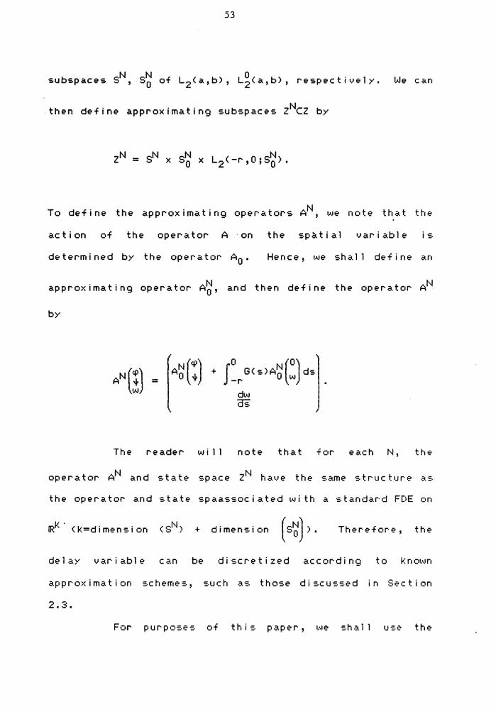
subspaces SN, SN0 of L..,<a,b), L~.<a,b), respectively. We can ~ ~

then define approximating subspaces zNcz by

zN = sN x s~ x L2<-r,O;S~).

To define the approximating operators AN, we note that the

action of the operator A ·on the spatial variable is

determined by the operator A 0 • Hence, we shall define an

approximating operator A~, and then define the operator AN

by

AN(~) = N (q:') rO N l'O) A0 ·¥, + • -r G<s>A0 w ds

dl,AJ as

The reader will note that for each N, the

opera tor AN and sta ta? space zN have the same structure as

the operator and state spaassociated with a standard FOE on

IRK· <l<=dimen:.ion (SN) + dimensic•n (s~')). Therefor·e, the

delay variable can be discretized according to Known

approximation schemes, such a:. those discu:.:.ed in :=:ection

2.3.

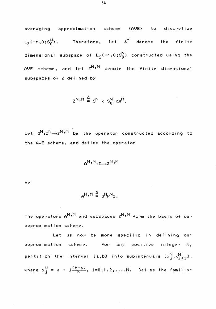
Fear purp•::i:.e:. c•f this. paper, 1,•.Je s.h.:c.11 us.e the

54

averaging approximation scheme <AVE> to di scret i ze

Therefore, 1 et ...s.M denote the finite

di mens i ona 1 subspace of L2 <-r, 0; S~> construe ted using the

AVE scheme, and let zN,M denote the finite dimensional

subspaces of 2 defined by

Let aM: zN-+zN ,M be the opera tor construe ted according to

the AVE scheme, and def i r1e the opera tor

by

The operators AN,M and subspaces zN,M form the basis of our

approximation scheme.

Let us now be more specific in defining our

approximation scheme. For any positive integer· N,

partition the inter•Jal [a,bJ into subintervals [x~,xjl+ 1 J,

\AJhe re xi';' = J

a + . < b-a) J N ' .j=O, 1,2, ••• ,N. Define the familiar

55

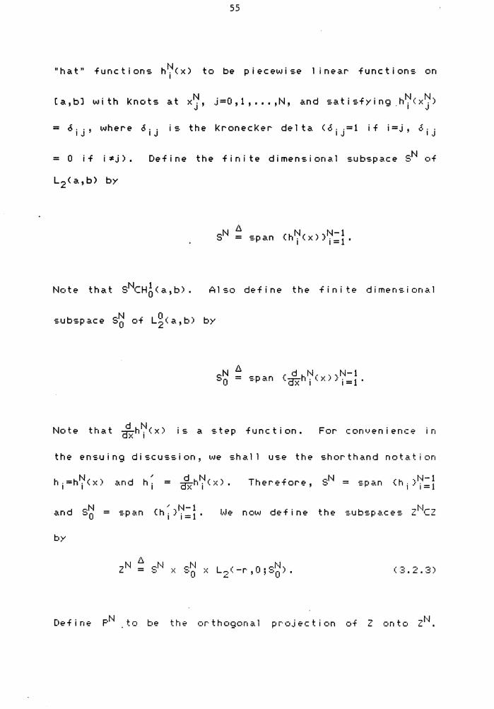
"hat" functions hr:(x) to be piecewise 1 inear functions. on

Ca,bl with Knots at x~, j=0,1, ••• ,N, and satisfying .h7<x~)

= 6 i j, where ~ i j is the KronecKer de 1 ta < -5 i j=l if i =j, o i j

= 0 if i$j). Define the finite dimensional subspace SN of

Also define the finite dimensional

subspace S~ of Lgca,b> by

b. SN = o;.p"'n { d hN"xl ,N-1 0 - "" dx i"' .Ji=l'

Note that Jxh~'<x> is a step function. For convenience in

the ensuing discussion, we shall use the shorthand notation

and s~ = span

by

/ -N-1 {hi}i=1"

Therefore, SN = s.pan ri. -~N-1 "'' i. i =1

l,Je nc•w define the -:.ubs.p~.ces. zNcz

(:3.2.3)

Define pN to be the C•r·thogonal pr·ojection of z C•nto zN.

56

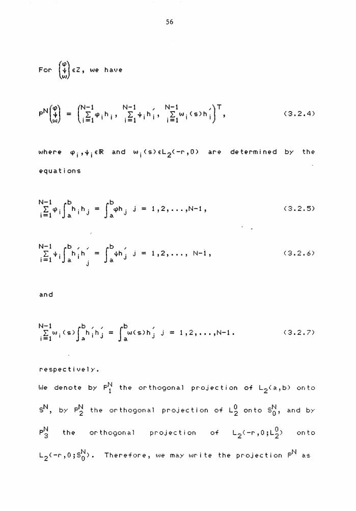
For (!) E:Z, we have

'N-1 N-1 ,. N-1 ,.)T = l2:cp.h., 2:-f·h., :Lw.(s)h. ,

i=l I I i=1 I I i=1 I I

equations

N-1 rb J.b 2: cp. h.h. = cph. j = i=l '~a 1 ·-' a J

1,2, .•. ,N-1,

N-1 I b ,. ,. 2:1·· h.h

i=1 I a I · J

fb ,. = ·¥h . j =

a J 1 , 2 , ••• , N-1 ,

and

N-1 f b ,. ,. 2:•,1.1.(s) h.h. j =1 I .;'c I J

J.b ,. = IAl(S)h · j =

a J 1,2, ••• ,N-1.

re~.pec ti ve 1 >".

(3.2.4)

(3.2.5)

(3.2.7)

I.Ne denc•te the or· thogc•na 1 pr·oj ec ti c•n of L~.< .:c., b) on to L .

N P~.

L the or· th c•gon .::c. l projection of Lg onto S~,

the or· thogona 1 pr·c•j ec ti c•n of L , - Ln) .-. 1 .. -r, LI: :-.. L ' L

on tc•

L2 <-r,O;S~). Therefore, we may write the projection PN as

57

Next we define operators A~ on SN x S~ which "approximate"

the opera tor A 0 • Since SN x S~ ¢ B<A0 >, we cannot define

by r-estricting A0 x .-.N 00' using the

framework of Section 2.4 <which in this case is similar to

the finite element method>, we define the bilinear form cr 0

The operator A~ is defined as a restriction of cr 0 to SN x

T"l(AN) = {l"~:)i:_7N.. Hl< Ot•,....N) i.: .-1'"' WI!: -r·, ,-=·o'

l0'-J1

(3.2.8)

58

AN(!) = [A~(:) + f~~(s)A~(~)dsl'. as

(3.2.9)

As mentioned above, for each N the operator AN has the same

structure as the reduced evo 1 u ti on opera tor:. a:.s•::ic i a ted

,,.., i th FDEs on IRK. Therefore J each AN, N=1, 2,... i :. the

infinitesimal generator of a c0 -semigroup TN(t) on zN <see

[ 5J, [ 19) >, and we can use the A'v'E approximation ideas.

For each positive integer, M, partition the

interval C-r,OJ into subintervals

J·-1 ~ M where tMJ. = -~. - ,..:., ... , ' ... characteristic function on the interval

M M [t.,t. 1) J ~'-

M M [t.,t. 1 > for J ..1-

j=2,3, ... ,M, and let x~ denote the characteristic function

M M on [ t 1 , t 0 J • Define the finite dimensional subspaces .s..M •:if

L ' 0 • .-.N) b 2~ -r' '-=-o · Y

~M N M M M ~ = C~€L~(-r,O;Sb>: ~ = r v ·X·,

~ . J=l .J .J VM-sN-.. . .i I:;·- o-· '

and define the finite dimensional subspaces zN,M of Z by

59

Next define the ope I" a tol"s a~'l: zN-.zN ,M by

wher·e

and

M b. M G. = J I"

tf':l f J-lw(s)d-:.

tl".1 J

fol" j=1 ,2, ••• ,M.

Define the opel"atol"s AN,M:z-.zN,M by

REMARK 3. 2 • 1

(3.2.10)

(3.2.11)

(~:.2.12)

and opera.tor·:. AN,M appr·ox imate the :.pa.ce Z and c•per·atc•r A

in the sense that the hypotheses of the Trotter-Kato

Theorem are satisfied. In part i cu 1 ar , th i :. require·:.

pr·ov i ng tha. t as N and M ~ 1:0

llAN,Mz - Azll _. 0

fc•r al 1 z in :.ome den:.e :.u b:.e t of D·< A) • From the triangle

60

inequality, we see that

Elementary spline estimates imply that s 2 -+ 0 as N-+ co

for each z, but convergence of the AVE scheme implies only

that s 1 -+ 0 as M-+o> for each fixed ~ and £.· In

part i cu 1 ar, the rate of convergence in M of AN ,M to AN i :.

N bounded by llA0 11. Al though A0 is an unbounded operator, we

w i 11 show that llA~ll=e"<N> <Lemma 3. 2. 5). We must ther1

choose the index M il .Z:. function of N so that the

convergence in M dominates the unbounded behavior of llA~ll.

This w i 11 require the somewhat de ta i 1 ed error estimates

found in the rest of this section.

Let fE:C(a,b). For each N, we denote the unique

continuous piecewise 1 inear interpolate of f by f7(x)

That i s, f~1 <xi > = f (xi ) for = 0,1, ... ,N, and f~1 <x) i:.

linear on each interval [xi-l'xil for i = 1,2, ••• ,N. 1,.Je

recal 1 the following wel 1-Known con~Jergence result for

interpolating 1 inear splines <see [21l, Theorem 2.5).

THEOREM 3.2.1 There exist fixed constants K1 ,K2 such that

61

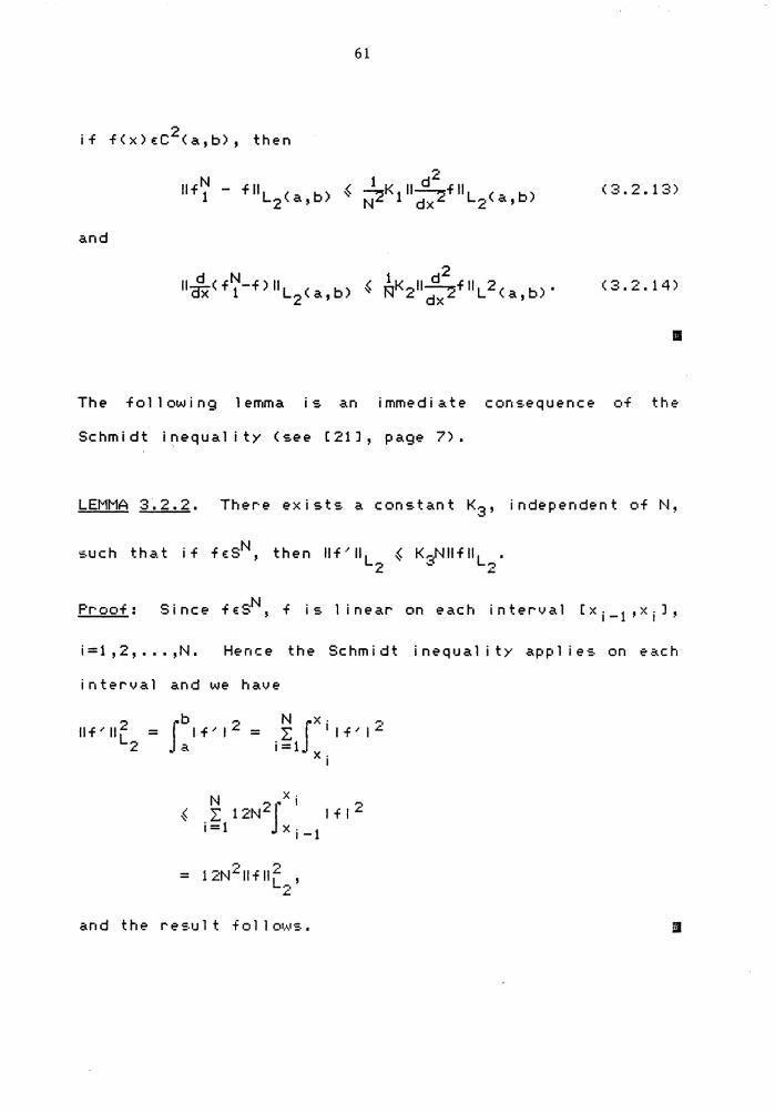
if f(x)€C2 <a,b), then

N 1 d2 II f 1 - f II L < a b) ~ ~K 1 ll~f II L < _ b)

2 ' N dx 2 ~, (3.2.13)

and

d N 1 d 2 llcrx< f 1 -f) II L2 (a' b) ~ f\JK2ll dx 2f II L 2 (a' b) • (3.2.14)

• The fol 1 owing 1 emma is an immediate consequence of the

Schmidt inequality <see [21J, page 7),

LEMMA 3.2.2. There exists a constant K3 , independent of N,

such that if f E:SN, then llf" II L ~ K~llf llL • 2 "" ,..,

~

Proof: Since fE:SN, f is linear on each interval rxi_ 1 ,xiJ'

i =1, 2, ••• ,N. Hence the Schmidt i nequa 1 i ty app 1 i es on each

interval and we have

2 llf"llL2 = Jblf"l2 = -~ Jxilf"l2 a 1=1

xi

N xi ~ .L 12N2f lfl 2

1=1 x. 1 1-

-:. ':' = 12N""llfllL.-.' J:.

and the result follows. 11

62

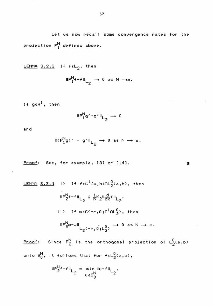
Let us now recall some convergence rates for the

projection P~ defined above.

LEMMA 3.2.3 If ftL2 , then

If gtH 1 , then

and

II < PN1 g) ' - ci,. II -+ 0 as N -+ -x- • - L,.., ..:.

Prc•of: See, for example, [3J or [14J.

N 1 d llP 2f-fllL ~ nK-.11-::r.:-fllL • 2 l'l .(;. ux 2

i i ) 1 fl If lAJE:C(-r,O;C flL.;), then • .<..

Pr·oof: .-. ,· n-e PN ~ r.... ,..., ..:. i -:. the projection

llF'~f-f II = ..:. L., L.

II

63

Define F(x) = b. Ix f(s)ds. Since the spline interpolate of F a

satisfies d<FN) €SN it follows that Ox 1 0'

where the last inequa.lity follo1,o..is. from (3,"2.14). The

res.ult ii) fol 1 ows from i) and the dc•mi nated con•.,ier•;ience

theorem. Thus the lemma is proved.

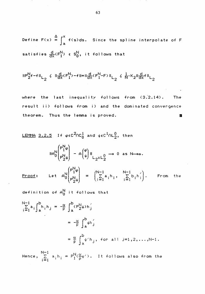
LEMMA 3.2.5

Let

If ,.~e:c 2ric 01 and ·'· -r·1nL 0 then ~ .,.~-· 2'

=

-+ 0 as N-+co.

"N-1 l "'> a.h .• .i~l I I.

N-1 ") I b. h .• i=l I I

definition of A~ it follows that

N-1 b I a-J h-h· = i=l I a I J

.b _(;(J i··i. - - .,,·II·• p .:.. .J .

Fr eirr1

M-1 Hence, I

i=l .:i_. h.

I I It follows also from the

II

the

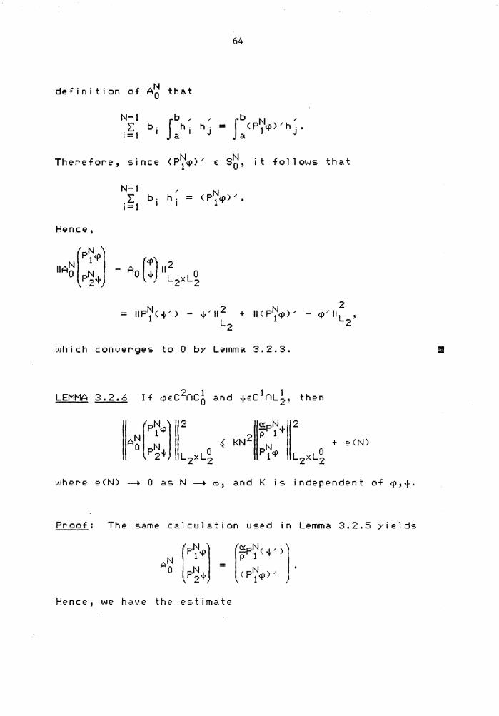
definition of A~ that

N-1 L: bi

i=1

Therefore, s i nee ( P~.;p) /

Hence,

64

it follows that

which converges to 0 by Lemma 3.2.3.

tN~l -· ~PN{· 2 .I:.

N 1 ...... p 1

Ao P~{· {~ KN'° pN + e 0--J)

n 1 .;p n L-.xL.:.. L.....,xL.:.. .J:. ~ .I:. .I:.

~"•here e(N) --+ 0 as N --+ oo, and K is independent of q:i ' ·~· •

Proof: The same calculation used in Lemma 3.2.5 yields

Hence, we have the estimate

65

2 2 ~ 2{ II~< P~+> ·'II + II ( P~cp) II + ll~[(P~t>; - t;Jll2 + ll~c+;-P~<·l·'>ll2}.

Now apply Lemma 3.2.2 to the fir·st h•Jo ter·ms, and Lemma

3.2.3 to tJ1E' las.t two terms, and the result follows. a

Si nee g E: H 1 , it fol 1 ows from standard arguments.

(i.e. see the proof of Corollary 3.1 in [2J) that there is.

a constant K<g> such that

0 M f I I gt:\t~( s)-g( s) I 2 ds ~ ~. -r i=1 1 1 M"-

Consequently, for each N ~ 0 there is an M 1 <N) = M1 s.uch

that

M ...,J.O 1 M1 M1 ,...,

1 i m N 4 I I g X < :.)-g( s) I 4 ds. = 0. N---to::- -r i = 1 i i

(~:.2.15)

It i :. imp or· tan t tc• nc•te that if M1 (l'D = Np for P> 1, then

ci. :. N ---+ ,o . On the other hand, for· s.pec i al form:. of •;;-i(s),

66

M1 <N> does not have to be unbounded. For ex amp 1 e, if g( s)

E c, then M1 <N> E 1 suffices to ensure (3.2.15>.

LEMMA 3. 2. 7 There exist con~.tants m.,13 ~.uch that for all

By Lemma 3.1.5, it is suffi•:ient to shc•v..1 that

<LAN,MLz,z>~1311zll 2 for all ze:Z. Therefore, let (!)i::z and

Consequently we have the equality

67

An argument ana 1 ogous to the one used in the pr-oof C•f Lemma

3.6 in C2J, <in which the AVE scheme is shown to sati~.fy

the ~.tabi 1 i ty hypotheses H1 of the Tr-otter--Kato Theor·em),

yields

(3.2.16)

Consider-ing the term s 1 we have

The Cauchy-Schwar-z inequality yields

Since M ~ M1 <N>, i t f o 1 1 ow s f,.. om Le mm a 3 • 2 • 2 , t he

Cec.u ch y-Sc h~·Jar· z i nequa 1 i ty, and the

that

(~:.2.17)

68

The equations (3.2.16) and (3.2.17) yield the result. m

In order to prove the remaining hypotheses of the

Trotter-Kato Theorem, define the dense subset D of BCA> by

D = { (!) e: 8( A) : (3.2.18)

Clearly D is den-:.e in B<A>, hence in z. The next lemma

shows that the consist ency condition H2> is sat i s.f i ed.

LEMMA 3.2.S Define the index M<N> such that

(~:.2.19)

and

(3.2.20)

If D i -:. def i n e d by ( 3 . 2. 1 8) , then AN' M < N) z -+ Az a·:. N-+,o

f c•r· a 1 1 z e: D •

Pr·oof: •'q:i) If z = l·i·

llJ, e: D, then

- Jo -i'·=)ll ~ M[rFN·•JM - EFN•JJM]-·· - di,_\)112 ,j<=_. ':J " -· · I . L, r: :~!"'· J. -1 3"' J. ..t i -::;-:; L -r· ._1=1 - ' u·=· 2

s,.., • ..;,

69

Lemma 3.2.5 implies s 1 -+ 0 as N-+ co. For the term s2 , we

have that

0 ( 0) (0 )'"' + J""'.r I G< s) I • llA~ P~~\I( s) - A0 w< s) I( ds

The domino. ted convergence theorem and Lemma 3. 2. 5 imp 1 y

that F 2 -+ 0 as N -+ co. For the term F 1 ~ applying first

the Cauchy-Schwarz inequality and then Lemma 3.2.6 yields

where e(N) -+ 0 as N-+ co. Hence, by (3.2.15) F 1 -+ 0 as M

-+ co, from which ~\le cone 1 ude that S--:- -+ 0 as. N -+ ,o. Fc•r

the term s3 , we have the estimate

c ,, ._•3·~

....

70

Observing that ~P~w = P~(~), Lemma 3.2.4 implies that E2

-+ 0 as N -+ o00. For the term E 1 , we follow the argument

used by BanKs and Burns in the proof of Corol 1 ary 3.1 in

C2J. This leads to

where

'Y~ = J sup < II ( fsP~w) < e > - ( ~P~w) < T > II : e ' T € ( t 7 ' t 7 -1] )

~ sup <ll(~<e> - ~<T>)llL2: e,·u:(t7,t7_i))

and

K =sup <ll~<a>ll: 0E:C-r,OD.

Since N -+ co impl i~s that M<N> -+ oo, it fol lows from the

uniform continuity of~ on C-r,OJ that E 1 -+ 0 as N-+ r.o.

Therefore, s3 -+ 0 as N-+ o00 and the lemma is proved. m

The next lemma shor..<JS that hypothesis H3) of the

Trotter-Kato Theorem is satisfied.

LEMMA 3.2.9 If Di:. defined b>· (3.2.18>, then there exi:.ts

a real number l such that RCA-l>D is dense in Z.

Proof: Since A is the infinitesimal generator of a

c0 -semigroup, there exists a real number l such that given

71

(~) e:Z, the equation

<A-~) (!) = (~) (3.2.21)

l'~) has a unique solution ~ e: ~<A>.

If (~) b,

e: S = C<a,b) x ctnLg x Ht<-r,O;Lg) <which is dense

,, q:i) in Z>, then the solution l~ e: ~(A) of (3.2.21) satisfies

0 ~+' + 1 J g<s>w'(s)ds - ~ q:i = ~ p p -r

dlAI = dS - ),lAJ Z o

Since and 13 e: ct' (3.2.23) implies

(3.2.22)

(3.2.23)

(3.2.24)

that -.2 q:• €: L. •

S .. 1 1 . Ht, c Lo) - d Ht ( l-1) ·Lo) ('-. ~. ~.4· 1m1 a r y, s 1 n c e we: ~ -r , " ; 2 .;e.n • z .;: -r· , , 2 , .:· . ..::. . ..::. .)

implies that •>Je:Ct<-r,O;L~>. . L.

Also, (3.2.22) imp 1 i es that

ti:: Ht and hence l't) i:: D • 1,~I

Therefc•re, the range of A-·1

contains the dense subset S, and the result follows.

The previous lemma<.:. imply that our apprc•ximati•::in <.:.cheme

satisfies the hypothe<.:.e<.:. c•f the Tr·ot ter-l<a t•:• Theorem. l.•.le

summarize the result in the following theorem.

THEOREM ::: • 2. 1 0 Let the inde-x M(N) be de-fined s•::i that

72

(3.2.19) and (3.2.20) hold. If the sequence of opera tors

b. is defined by aN = AN ,MO'-'), then the

hypotheses of the Trotter-Kato Theorem hold; that is,

<f"<t> !..+T<t),

uniformly on compact t in ter·va 1 s, wher·e <f"< t) is. the

semigroup generated by aN. Ill

Assuming that the approximation scheme <ZN,PN,aN) and index

M<N) are defined as in Theorem 3.2.10, let us consider the

d . d . . t . t . h ( -LN F.N ..,N* ~. corl"'espon 1 ng a JOI n approx 1ma 1 on s.c eme . , , 1.~ J.

Since llTN*<t)ll = llTN(t)ll, it follc•ws fl"'om Lemma 3.2.7 that

hypothesis Hl) of the Trotter-Kato Theorem is satisfied by

the adjoint approximation scheme. We note that s. i nee.

= AN - 0'

apply to

it

AN* 0 •

fol 1 01,\JS that

Combining

the es.ti mates. in Lemma 3. 2. ~.

this. obs.erva ti on with the

conve!"gence rates for the approximating ad..i•:iint oper·atc•r·s.

in the AVE scheme (see CllJ>, it follows that

for all z~o*. Here o* is the dense subset of F<A*> defined

bv ..

Arguments completely analogous to those used in the proof

73

of Lemma 3.2.9 yield that hypothesi:. H3) holds for· the

adjoint approximation scheme. From these observations we

cone 1 ude the fol 1 c•w i ng.

Corollary 3.2.11 I f th . t . h { 2 N ' pN ' aN) . e approx1ma ion sc eme 1s

defined as in Theorem 3.2.10 then

uniformly in compact intervals. g

Therefore, we conclude <see Section 2.2) that our

approximation :.cheme :.hould prove reasonable

approximating the optimal contrcol problem ass•::iciated 11.Jith

the viscoelastic system (3.1.3)-(3.1.6). In the ne;<t

chapter we di:.cuss some of our numerical re:.ult:. fcor· thi:.

problem.

CHAPTER IV

4.1 ~viscoelastic model

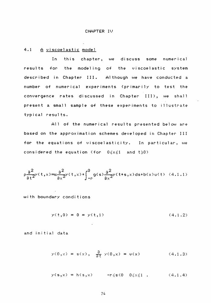
In this chapter, we discuss some numer i ca I

results for the modeling of the viscoelastic system

described in Chapter I I I. Al though we have cond•Jc ted a

number of numerical experiments (primarily to test the

convergence rates discussed in Chapter III>, we shall

present a sma 11 sample of these experiments. tc• i 11 us.tr.:.. te

typical results.

All of the numer i ca 1 results pres.en ted be I ow ar·e

based on the approximation schemes developed in Chapter III

for the e qua t i on s of v i sc oe l as t i c i t y • In particular, we

considered the equation (for O~x~1 and t~O)

with boundary conditions

y(t,0) = 0 = y(t,1) (4.1.2)

and initial data

y(O,x) = s.(x), :3 = n y<O,x) v<x> (4.1.3)

y(s,x) = h<s,x) (4.1.4)

74

75

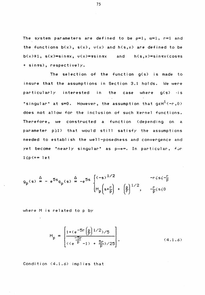
The system parameters are defined to be p=l, <X=l, r=l and

the _functions b<x>, s<x>, v<x> and h<s,x) are defined to be

b<x>=l, s<x>=sin~x, v<x>=~sin~x and h<s,x>=sin~x(cos~s

+ sin~s>, respectively.

The selection of the function g<s> is. made tc•

insure that the assumptions in Section 3.1 holds. We were

pa.rticularly interested in the case where g(s) ·is.

"singular" at s=O. However, the as.sumption that g€H 1<-r·,0)

does not a 11 ow for the inc 1 us ion of such Kerne 1 function: .•

Therefore, we constructed a function (depending on a

para.meter p~l) that •.AJould still satisfy the as·:.umptions

needed to establish the well-posedness and convergence and

yet become "nearly singular" as p~•0 , In particular·, +.:..1r

l~p<+~ let

5~. = -e

where M is related top by

Cc•nd it i •:in ( 4. 1. 6) imp 1 i es. that

l(.2.)1/2 r '

(4.1.6)

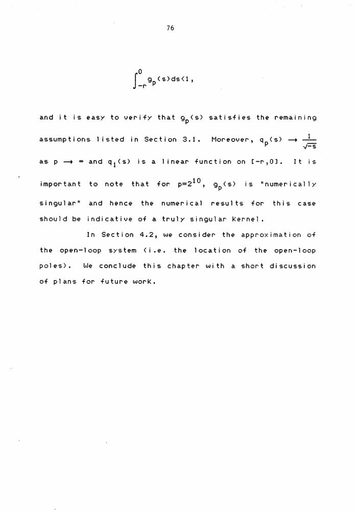
76

0 I g (s)ds<1, -r p

and it is easy to verify that gp(s) satisfies the remaining

assumptions 1 isted in Sect i on 3. 1 • Moreover, --+

asp--+ - and q 1<s) is a linear function c•n [-r,OJ. I t i :.

important to note that for p=2 10 , gp(s) is "numerically

s i ngu 1 ar" and hence the numer i ca 1 resu 1 ts for this ca:.e

shc•uld be indicative of a truly singular ker·nel,

In Section 4.2, we consider the approximation of

the open-1 oop system (i.e. the 1 ocat ion of the open-1 oop

poles). We conclude this chapter with a short discussion

of plans for future worK.

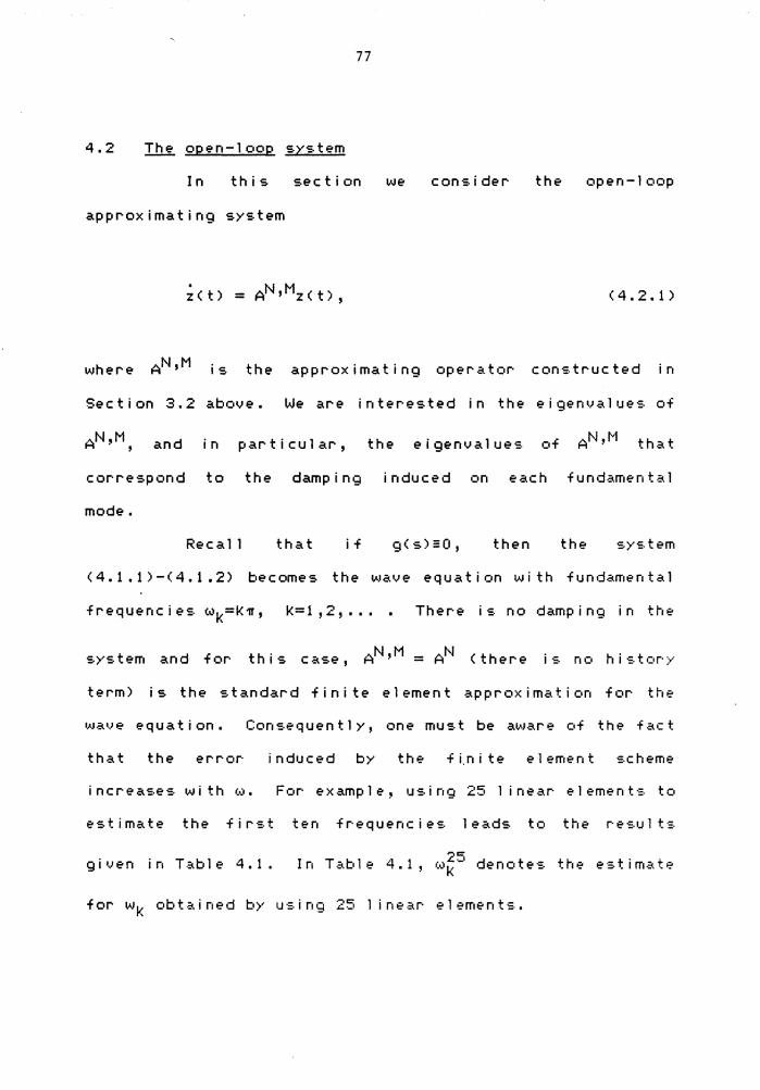
77

4.2 The open-loop system

In this section VJe consider- the open-loop

appr-oximating system

(4.2.1)

wher-e AN ,M is the appr-ox i mating op er-a tor- con-:.tr-uc ted in

Section 3.2 above. We ar-e inter-ested in the eigenvalues of

AN,M, and in par-ticular-, the eigenvalues of AN,M that

cor-r-espond to the damping induced on each fund.:c.men t~. l

mode.

Rec a 11 that if g(s)EO, then the =·>'=· t em

(4.1.1)-(4.1.2) becomes the 1,.<Jaue equation with fundamental

fr-equencies wk=K~, k=1 ,2, ... Ther-e is no damping in the

system and for- th . AN,M =AN 1 s case, <ther-e is nc• hi:.tor·::."

ter-m) is the standar-d finite e 1 emen t appr-ox i mat i c•n for- the

wave equation. Consequently, one must be awar-e of the fact

that the er-r-or· induced by the f i.n i te e 1 emen t :.cheme

incr-eases with w. For example, using 25 1 inear- elements to

estimate the fir-:.t ten fr·equencie:. leads to the r·e:.1Jlt·:.

given in T.:c.ble 4.1. I T t 1 4 1 25 d t +I-n a • e · • , (vk en o es .11 e e·:.timati:-

for- wk obtained by using i near· e 1 emen t: ..

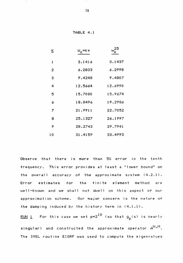
78

TABLE 4 .1

K W -K'll' K- ,25 µ K

3.1416 3 .1437

2 6.2833 6.2998

3 9.4248 9.4807

4 12.5664 12. 69'7'0

5 15.7080 15.9674

6 18.8496 19.2986

7 21 . 9911 22.7052

8 25.1327 26 .1997

9 28.2743 29.7941

10 31.4159 33. 49'7'3

Observe tha. t there i :. more than 5% error in the ten th

frequency. Thi:. error pr-ovide:. at lea:.t a "lotA.•er- bound" on

the over·all accurac>' of the approximate sy:.tem (4.2.1).

Error e:.timate:. for- the finite element met h cuj .:i.r· e

approximation scheme. Our major concern i -:;. the nature of

the damping induced by the history term in (4.1.1).

RUN 1 thi:. ca:.e we :.et P=2 1 O ( :.c• that Q ( :.) i :. nea.r· 1 y -p

singular) and c•:•nstructed the appr·c·ximate oper.:c.tor· At··~,M.

The IMSL routine EIGRF was used to compute the eigenvalues

79

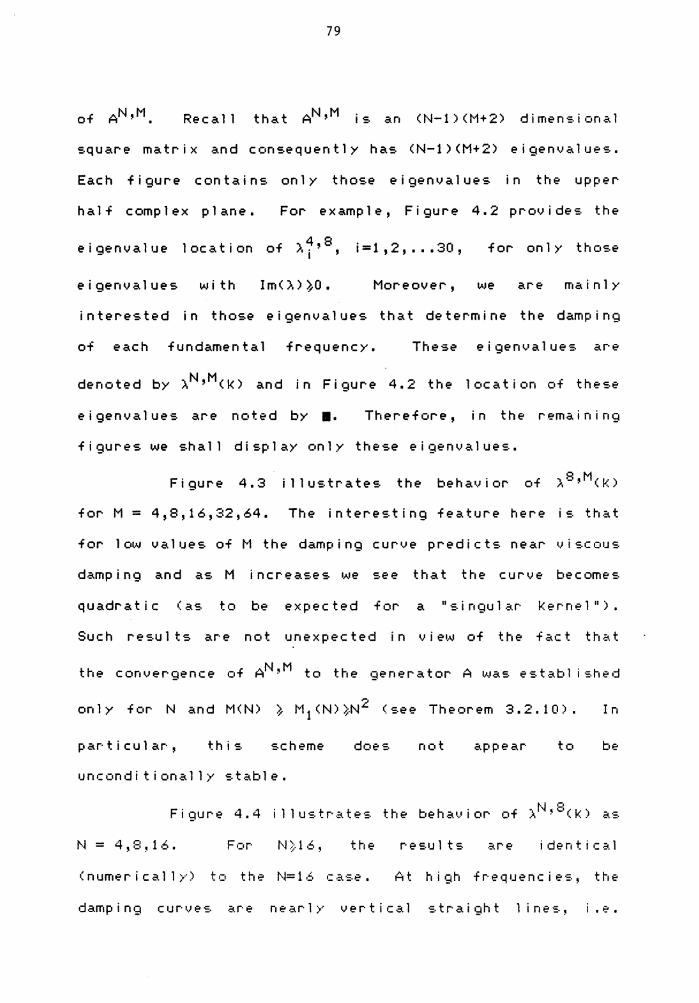
Recal 1 that AN,M is an <N-D<M+2) dimensional

square matrix and consequently has <N-1><M+2) eigenvalues.

Each figure contains on 1 y those e i genva 1 ues in the upper

half complex plane. For example, Figure 4.2 provides the

eigenvalue location of ).~' 8 , i=1,2, ••• 30, I

for on 1 y those

eigenvalues with Im<:>.> ~o. Moreover, we are mainly

interested in those eigenvalues that determine the damping

of each fundamental frequency. These eigenvalues are

denoted by ).N,M<K> and in Figure 4.2 the location of these

e i genva 1 ues are noted by •· Therefore, in the remaining

figures we shall display only these eigenvalues.

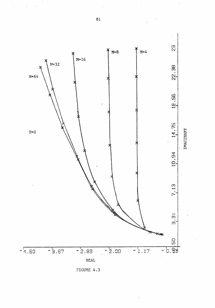
Figure 4.3 illustrates the beha~)ior of ). 9 ,M(K)

for M = 4,8,16,32,64. The interesting feature here is that

for 1 ow va 1 •Jes of M the damping curve predicts near vi sco•Js

damping and as M increases we see that the curve becomes

quadratic <as to be expected for a "singular Kernel").

Such resu 1 ts are not unexpected in vi e•AI of the fact that

the convergence of AN,M to the generator A was established

only for N and M<N) ~ M 1 <N)~N2 (see Theorem 3.2.10). In

par·t i cul ar, this scheme does not appear to be

unconditionally stable.

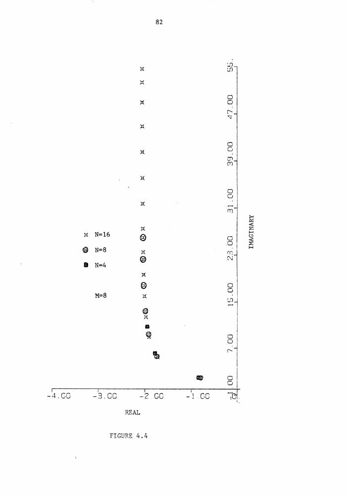
Figure 4.4 illustrates the behavior of ).N,S(K) as

N = 4,8,16. the re~:.ults are identica.l

( n ume r i ca 1 1 »-> ti::i the N= 1 6 c .a se • At high frequenc i e:., the

damping curve:. ar·e nearly vertical straight line:., i.e.

80

•

N=4

M=8

•

D-O o.., -,

I I

oi ,..... I .__. I . -;

cc !

I i

0 1,' ~ 01<

·J ~ LDIO ;;

I 1-1

r c! O! ·j ~I

I

' I I

cl o!

B Ni !

c 0

r~~~~~,,--~~~~~,~~~~~~~~~~-~~,~~----,):0;.!(,--~~=-~

- 1 l . cc -9. co - 1. oo -5. oo -3. oo - 11 . cS I REAL

FIGURE 4.2

H

~ Cl . H z

~

,_. w

-0 . tD A

-A . ...,.] CJ1

,_. m . CJ1 m

N N

w cc

N Ul

f]=W

,.....,... . _, uu (., - I

8=W

1Vffil

ss·z ... lS"E-os· v - I ' '

8=H

179=H

91=W

18

17·17 3:Cl.fl~ H

1Vffil I

'E-ClQ . 1 -ClCl z-ClCl. E-Cl'J' 17- I I I I

I ci @

10 I I ~

l I .......)

r· 10 ® :O

I m I }:( I ® k; ):( B=:W.

0 ® 0

}:(

® 17=N

• !\) ~) ):(

B=N ® H ! er ~ lo ® CJ 91=N ):(

H :z: ):( > ~

(.;)

}:(

Cl 0

):(

~w ill

18 ):(

t. ......)

0 0

):(

en -(,'i ):(

Z8

83

representative of pure viscous damping. Again, th i s.

illustrates the need to construct an approximate model

with to insure that the finite

dimensional model ci.ccurately predicts the damping prc•duced

by the history term.

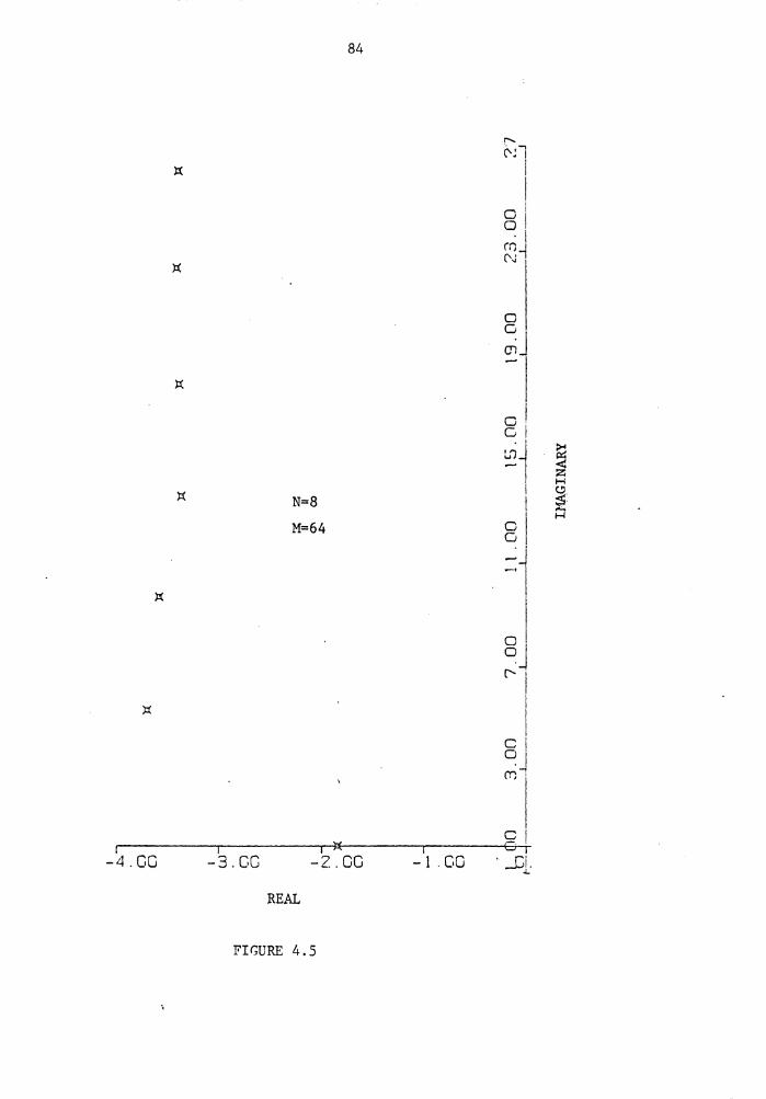
RUN 2: The results illustrated in Figures (4.2)-(4.4) are

typical of the many numerical experiments that we conducted

us.ing various. par·ameter·s and Kernels gp(s) fc•r lar·ge p. In

order to determine the effect of a non-singular Kernel, we

reproduced the N=8, M=64 re-:.u 1 t:. fc•r the Ker·ne 1 func ti c•n

g,....( s.) • "-

Figure 4.5 contains the eigenvalue locatic•n:. fc•r

this. S.)":.tem. Again • .. \le :.ee that the apprc•xim~.te mc•del

predicts purely viscous damping in the high frequency

modes. This run illustrates the importance of the singular

Kernel in the modeling of structural damping at high

frequency.

H ..... ·~ 'Q H z > ~

16

1{.;J

1· .0 18 I

I I

I -..) ro lo ~~ j8 I I

~~ I C) io

'\) h.:J I . 10 lo

I L~v -....J

oo·z-oo·s-

179=W

B=N

178

85

4.3 Concluding remarks

In this paper, we considered we 11-posednes:. and

approximation schemes for a c 1 ass of func ti ona 1 part i a 1

differential equations of hyper-bol ic type. Our :. tudy v.ias

motivated by the desire to construct state space models and

convergent finite dimensional approximate model:. :.uitable

for control design. Therefore, we first developed a

gel)eral algorithm for con:.tructing finite dimen:.ional

systems that approximate well-posed Cauchy problems and

their adjoints. We then established the well-posedness of

the Boltzmann model for- viscoelasticity in the state space

and used this mode 1 to deve 1 op a

convergent numer i ca 1 scheme. vJe h ::.ve used this :.cheme tc•

simulate the system and to study the effects of the Kernel

on the damping in the :.ystem.

Our numer· i ca 1 resu 1 ts are pr·e 1 i mi nary, and ther·e

is much room for further study. For example;

1) We plan to test the approximation scheme on optimal

control problems for the viscoelastic model.

2) We p 1 an to use the "n ev..• -:.p 1 i n e :. " for di -:.c re t i z i n g the

heredi tar·y var· i able in c•ur approximation :.cheme, a:.

compar·ed tc• the "AVE" :.cheme which v.Je u:.ed in th i =· paper.

3) We plan to investigate the use of higher order

element:. •, 1 .e. cubic spline-:.) as a bas.is for· the

:.pat i al di :.c r· et i z at i c•n i n o•J r· ap pr· ox i mat i on -:.ch eme .

86

Pre 1 i mi nary runs indicate superior performance over

linear splines <Re: Table 4.1).

4) We are interested in extending our ideas to fourth

order <in the spatial variable) equations v..th i ch are

used to mode 1 beams. Pre 1 i mi nary ap p 1 i cat i on s to a

clamped-clamped beam have been successful.

5) In our proof of we 11 -posednes~., we made the

res tr i c t i on 1 -ge:H ( r,O>. This exc 1 udes s i ngu 1 ar

Kernels, which are imp or tan t. Thus we are

investigating well-posedness results which allow for

singular Kernels.

6) We plan to investigate boundary conditions other than

the Dir i ch 1 et bo•Jndary cond i ti ons. For ex amp 1 e, to

mode 1 a s 1 ew i ng beam, other boundary cond it i c·n~. mu~.t

be considered.

REFERENCES

1. Aubin, ,J.P., Applied Functional Analysis, W i 1 ey lntersciences, New YorK, (1979).

2. Banl<s, H.T. and Burns, J.A., Hereditary control problems: numerical methods ba:.ed on averaging approximations, SIAM J. Control Optimization, Vol. 16, (1978), 169-208.

3. BanKs, H.T. and Kappel, F., Spline approximation for functional differential equations, J. Differential Equations, Vol. 34 (1979), 496-522.

4. Banl<s, H.T., Rosen, I.G., and Ito, K., A spline based technique for computing Riccati operators and feedback controls in regulator problems for delay equations, SIAM J. Scientifi'c Statistical Computing, lJol. 5 <1984), 830-855.

5. Cl i ff, E .M. and Burns, J .A., parameter identification of IF IP, N. Y. , < 1 981 ) •

"Reduced approximations in hereditary systems", Proc.

6. Curtain, R.F. and Pritchard, A.,J., Infinite Dimen:.ional Linear Systems Theory, Springer, Berl in (1978)~

7. Di8lasio, G., The linear-quadratic optimal control prc•blem for delay differential equations, Rend. Accad. Naz. Lincei, 71 ( 1981)' 156-161 •

8. DiBlasio, G., Kunisch, K., and Sinestrari, E.,

9.

10.

L 2 -Regu 1 ar i ty for parabol i c part i a 1 in tegrod i fferen ti a 1 equations with de 1 ay in the hi ghest-or·der· der i tJa ti ve:., J. Math. Anal. Appl., 102 (1984), 38-57.

DiBlasio, G., for abstract preprint.

Kunisch, K., and Sinestrari, E., Stability 1 inear functional differential equations,

Gibson, J.S., The Riccati integral equations control problems on Hi 1 ber t :.paces, SIAM ,J. t,,101. 17·, No. 4, <1979), 537-565.

for c•p t i ma 1 on Control,

11. Gibson, J.S., Linear quadra.tic optimal control c•f hereditary differential systems: Infinite dimensional Ricca ti equations and numer i ca 1 approximations, SIAM ,J. Cc•ntrol Optim., 21(1983), 95-139.

1 2. G i bson , ,J. S. , .:..n d Rosen , I • G. , Sh i ft i n g the c 1 o:.e d-1 c•op spectrum in the optimal 1 inear quadratic re9ul.:..tor· pr·c•blem for hereditary systems, preprint.

13. Hr·•J~.a, .:tnd Nohe 1 , .J.A., Global existence and

87

88

asymp tot i cs in one-di mens i ona l non l i near voscoe last i city, Proceedings of the 5th S>'mposium on application-:. of pure mathematics to mechanics, Springer l ec tu re notes in physics, Vol , 195( 1984), 165-187.

14. Kappel, F. and Salamon, D., Spline approximation for retarded -:.ystems and the Riccati equations, MRC Technical Report #2680, 1984.

15. Krein, S.G., Linear Differential Spaces, Transl. Math. Mono., 29, Society, Providence, RI, 1971.

Equations l.D. Banach American Mathematical

16. Kunisch, partial

K. and Schappacher, W., differential equations

Necessary conditions for with delay to generate

c0-sem i groups, .Journa 1 of Different i a 1 Equations, ·so ( 1983), 49-79.

17. Oden, .J. Tinsley, Aool ied Functional Analy:.i:., Prentice-Ha 11 , New Jersey, < 1979).

18. Pazy, A., Semigroups of .iQ. Partial Differential

Li near Opera tor:. and App 1 i c.:i. ti ons Equations, Spring~~, New York

(1983).

19. Powers, R.K., Chandras~Khar equations for di~.tributed

Department, Un i v er s i t :v·,

parameter systems, Ph.D Thesis, Mathematics Virgina Polytechnic Institute and State Blacksburg, VA (1984).

20 • Russe 1 1 , D. L. , Math ema t i cs of Fi n i t e Di mens i c•n .:..1 Cc•n tr· c• l Systems, Theory and Design, Marcel Dekker, N.Y. 1979.

21. Schultz, M.H., Spline Analy:.i:., Prentice Hall, EnglevJc•od Cliffs, N.Y. (1973).

22. Tr·.:i.vis, C. and Webb, G., Partial differential t"Ji th deviating arguments in the time variable, Ana 1 • App 1 • 56( 1976), 397-409.

equa ti c•ns J. Ma th.

23. Travis, C. compac tne:.~. differential 12$'-143.

.:i.n d l . .Je bb, G. , in the ~-norm

equ.:i.tii::::ins, Trans.

Existence, stabi Ii ty and for partial function~.!

Am. Math. Soc., 240(1978)

24. L•.Jalker, .J.A., DYn.:i.mi•:al Sy:.tem: .. :;..nd E\.icilutic•n Equations, Plenum Press, New York (1980).

The vita has been removed from the scanned document

APPROXIMATION OF

INTEGRO-PARTIAL DIFFERENTIAL EQUATIONS

OF HYPERBOLIC TYPE

by

Richard H. Fabiano, Jr.

<ABSTRACT)

A state space model is developed fo~ a class of

integro-partial differential equations c•f h>'perbol ic b'pe

which arise in viscoelasticity. An approximation scheme is

deve 1 c•ped ba:.ed on a :.p 1 i ne approximation in the spat i a.1

variable and an averaging approximation i n the de 1 a; .. ·

variable. T~chniques from 1 inear semi group theory are used

to discuss the well-posedness of the state space model and

the convergence properties of the approximation scheme. We

give numer·ical r·e:.ult-:. for a ·:.ample prc•blem to illu·:.tr·ate

some properties of the approximation scheme.