University of South FloridaScholar Commons

Graduate School Theses and Dissertations USF Graduate School

6-1-2008

Limits of beach and dune erosion in response towave runup from large-scale laboratory dataTiffany M. RobertsUniversity of South Florida

Follow this and additional works at: http://scholarcommons.usf.edu/etdPart of the American Studies Commons

This Thesis is brought to you for free and open access by the USF Graduate School at Scholar Commons. It has been accepted for inclusion in GraduateSchool Theses and Dissertations by an authorized administrator of Scholar Commons. For more information, please contactscholarcommons@usf.edu.

Scholar Commons CitationRoberts, Tiffany M., "Limits of beach and dune erosion in response to wave runup from large-scale laboratory data" (2008). GraduateSchool Theses and Dissertations.http://scholarcommons.usf.edu/etd/478

Limts Of Beach And Dune Erosion In Response To Wave Runup From Large-Scale

Laboratroy Data

by

Tiffany M. Roberts

A thesis submitted in partial fulfillment of the requirements for the degree of

Master of Science Department of Geology

College of Arts and Sciences University of South Florida

Major Professor: Ping Wang, Ph.D. Charles Connor, Ph.D.

Nicole Elko, Ph.D. Rick Oches, Ph.D.

Date of Approval: April 30, 2008

Keywords: beach erosion, nearshore sediment transport, swash excursion, wave breaking, physical modeling, surf zone processes, coastal morphology

© Copyright 2008, Tiffany M. Roberts

Acknowledgements

The support and guidance of those who have contributed to the successful

completion of this thesis have been greatly appreciated. Most importantly, I would like

to sincerely thank Dr. Ping Wang for his knowledge, instruction, and guidance during this

project. From guidance during my undergraduate Honors Thesis through the present, Dr.

Wang has been the most important and influential person in my academic, educational,

and personal advancements. I would also like to extend sincere thanks to Dr. Nicole Elko,

whose guidance through my thesis lead to a more comprehensive understanding of

coastal environments and processes. Her time and dedication to my academic

advancement played an instrumental role in the development and successful completion

of this thesis.

I would also like to thank Dr. Nicholas Kraus for the SUPERTANK dataset and

significant contributions to the study including insights into the broader implications of

swash processes in many different coastal applications. Thanks to my other committee

members, Drs. Chuck Connor and Rick Oches, whose contribution guided me towards a

more comprehensive analysis of this topic.

Finally, thanks to my family and friends who have supported me during my

educational endeavors with constant encouragement to pursue my academic and personal

aspirations and dreams. Thank you all.

i

Table of Contents

List of Figures ii List of Tables iv Abstract v Introduction 1 Literature Review 3 Methods 11 SUPERTANK and LSTF 11 Data Analysis 15 Results 18 Beach Profile Change 20 Cross-shore Distribution of Wave Height 31 Wave Runup 37 Discussion 42

Relationship between Wave Runup, Incident Wave Conditions, and Limit of Beach Profile Change 42 A Conceptual Derivation of the Proposed Wave Runup Model 56

Conclusions 60 References 62 Appendices 68 Appendix I – Notation 69

ii

List of Figures

Figure 1 Power density spectra from the LSTF experiment under spilling and plunging breakers measured from an offshore gauge (above) and a gauge at the shoreline (below). 7

Figure 2 Beach-type classification based on beach morphology and slope. 9 Figure 3 The SUPERTANK experiment (upper) and LSTF (lower) during

wave runs. 12 Figure 4 The first SUPERTANK wave run, ST_10A erosive case. 21 Figure 5 The SUPERTANK ST_30A accretionary wave run(upper). 24 Figure 6 The SUPERTANK ST_60A dune erosion wave run. 25 Figure 7 The SUPERTANK ST_I0 accretionary monochromatic wave run. 26 Figure 8 The LSTF Spilling wave case. 27 Figure 9 The LSTF Plunging wave case. 29 Figure 10 The cross-shore random wave-height distribution measured during

SUPERTANK ST_10A; yellow arrow indicates the breaker point. 31 Figure 11 The cross-shore random wave-height distribution measured during

SUPERTANK ST_30A. 33 Figure 12 The cross-shore random wave-height distribution measured during

SUPERTANK ST_60A. 34 Figure 13 The cross-shore monochromatic wave-height distribution measured during SUPERTANK ST_I0. 35 Figure 14 The cross-shore wave-height distribution and γ for the LSTF Spilling

and Plunging wave cases. 36

iii

Figure 15 Wave runup measured during SUPERTANK ST_10A. 38 Figure 16 Wave runup measured during SUPERTANK ST_30A. 39 Figure 17 Wave runup measured during SUPERTANK ST_60A. 40 Figure 18 Wave runup measured during SUPERTANK ST_I0. 40 Figure 19 Relationship between breaking wave height, upper limit of beach profile

change, and wave runup for the thirty SUPERTANK cases examined. 43 Figure 20 Comparison of measured and predicted wave runup for Eqs. (10), (4),

(6), and (7). 46 Figure 21 Measured versus predicted runup for Eq. (10), including the anomalies. 47 Figure 22 Measured versus predicted runup for Eq. (10), excluding the anomalies. 48 Figure 23 Measured versus predicted runup for Eq. (4), excluding the anomalies. 49 Figure 24 Measured versus predicted runup for Eq. (7), excluding the anomalies. 49 Figure 25 Measured versus predicted runup for Eq. (6), excluding the anomailes. 50 Figure 26 Figure 4c from Holman (1986) comparing swash runup (minus setup)

and offshore significant wave height (above); the digitized data from Figure 4 (Holman, 1986) with two linear regression analyses (below). 52

Figure 27 Figure 7c from Holman (1986) comparing swash runup(minus setup)

and the surf similarity parameter (above); the digitized data from Figure 4 (Holman, 1986) with a linear and exponential regression analysis (below). 53

Figure 28 Schematic drawing of forces acting on a water element in the swash zone. 57

iv

List of Tables

Table 1 Summary of Selected Wave Runs and Input Wave and Beach Conditions (Notation is explained at the bottom of the table). 19

Table 2 Summary of Breaking Wave, Maximum Wave Runup, Upper

and Lower limits of Beach-Profile Changes, and Presence of a Scarp for Each Analyzed Wave Run. 30

Table 3 Summary of Measured and Predicted Wave Runup Equations. 46

v

Limits of Beach and Dune Erosion in Response to Wave Runup from Large-Scale Laboratory Data

Tiffany M. Roberts

Abstract

The SUPERTANK dataset is analyzed to examine the upper limit of beach change

in response to elevated water level induced by wave runup. Thirty SUPERTANK runs

are investigated, including both erosional and accretionary wave conditions under

random and monochromatic waves. Two experiments, one under a spilling and one

under a plunging breaker-type, from the Large-Scale Sediment Transport Facility (LSTF)

are also analyzed. The upper limit of beach change approximately equals the maximum

vertical excursion of swash runup. Exceptions to this direct relationship are those with

beach or dune scarps when gravity-driven changes, i.e., avalanching, become significant.

The vertical extent of wave runup, Rmax, above mean water level on a beach without a

scarp is found to approximately equal the significant breaking wave height, Hbs.

Therefore, a simple formula max bsR H= is proposed. The linear relationship between

maximum runup and breaking wave height is supported by a conceptual derivation. This

predictive formula reproduced the measured runup from a large-scale 3-dimensional

movable bed physical model. Beach and dune scarps substantially limit the uprush of

swash motion, resulting in a much reduced maximum runup. Predictions of wave runup

are not improved by including a slope-dependent surf-similarity parameter. The limit of

vi

wave runup is substantially less for monochromatic waves than for random waves,

attributed to absence of low-frequency motion for monochromatic waves.

Introduction

Accurate prediction of the upper limit of beach change is necessary for assessing

and predicting dramatic morphological changes accompanying storms. It is particularly

important for coastal management practices, such as designing seawalls, nourishment

profiles, and assessing potential coastal damages. The upper limit of beach change is

controlled by wave breaking and the subsequent wave runup. During storms, wave runup

is superimposed on elevated water levels (due to storm surge). Wang et al. (2006) found

that the highest elevation of beach erosion induced by Hurricane Ivan in 2004 extended

considerably above the measured storm-surge level, indicating that the wave runup

played a significant role in the upper limit of beach erosion. The limit of wave runup is

also a key parameter for the application of the storm-impact scale by Sallenger (2000).

The Sallenger scale categorizes four levels of morphological impact by storms through

comparison of the highest elevation reached by the water (storm surge and wave runup)

and a representative elevation of barrier island morphology (e.g. the crest of the foredune

ridge). In addition, accurately assessing wave runup has numerous engineering

applications, including design waves for overtopping of seawalls, breakwaters and jetties,

and elevation of berm height for beach nourishment (Komar, 1998). Therefore,

quantification of wave runup and its relationship to the upper limit of beach-profile

change are essential for understanding and predicting beach and dune changes. Limit of

2

runup typically serves as a crucial parameter for the modeling of coastal morphology

changes.

3

Literature Review

Wave runup is composed of wave setup and swash runup, defined as a super-

elevation of the mean water level and fluctuations about that mean, respectively (Guza

and Thornton, 1981; Holman and Sallenger, 1985; Nielsen, 1988; Yamamoto et al., 1994;

Holland et al., 1995). Wave setup can be further defined as a seaward slope in the water

surface that provides a pressure gradient or force balancing for the onshore component of

the radiation stress induced by the momentum flux of waves (Komar, 1998). The swash

runup component of wave runup is defined as the upper limit of swash uprush. The

swash uprush is strongly modulated by low-frequency oscillations often referred to as

infragravity waves with periods of at least twice the peak incident wave periods (Komar,

1998).

Previous studies on the limits of wave runup were primarily based on field

measurements at a few locations resulting in several formulas developed to predict wave

setup and runup. An early formula for wave setup slope was based on a theoretical

derivation for sinusoidal, or monochromatic, waves on a uniformly sloping beach

(Bowen et al., 1968):

hKx xη∂ ∂= −

∂ ∂ 2 1(1 2.67 )K γ − −= + (1)

where h = still-water depth, η = wave setup, x = cross-shore coordinate, γ = H/(η + h)

and H = wave height. The term γ essentially describes the relationship between the

4

breaking wave height and its proportionality to local water depth. Based on both theory

and laboratory measurements, the maximum set-up under a monochromatic wave, Mη ,

was found to occur at the still-water shoreline (Battjes, 1974):

0.3M

bHη γ= (2)

where Hb = breaking wave height. The above equations concern only the setup

component of the entire wave runup, not including the portion of elevated water level

induced by swash runup. Taking the commonly used value of 0.78 for γ, the maximum

setup yielded from the above equation is about 23% of the breaking wave height.

Based on field measurements conducted on dissipative beaches, Guza and

Thornton (1981) found maximum setup at the shoreline, slη , to be linearly proportional

to the significant deepwater wave height, Ho:

0.17sl oHη = (3) Guza and Thornton (1982) found that the significant wave runup, Rs, (including both

wave setup and swash runup) is also linearly proportional to the significant deep-water

wave height:

3.48 0.71 (units of centimeters)s oR H= + (4) Comparing Eqs. (3) and (4), the entire wave runup is approximately 4 times the wave

setup, i.e., swash runup constitutes a significant portion, approximately 75%, of the total

elevated water level. According to Huntley et al. (1993), Eq. (4) is the best choice for

predicting wave runup on dissipative beaches. Based on field measurements on highly

dissipative beaches, Ruessink et al. (1998) and Ruggiero et al. (2004) also found linear

relationships, but with different empirical coefficients.

5

Based on field measurements on both dissipative and reflective beaches, Holman

(1986) and several similar studies (Holman and Sallenger, 1985; Ruggiero et al., 2004;

Stockdon et al., 2006), argued that more accurate predictions can be obtained by

including the slope-dependent surf-similarity parameter, ξ:

1/ 2( / )o oH Lβξ = (5)

where Lo = deepwater wavelength, and β = beach slope. The surf similarity parameter

has been broadly used to parameterize many nearshore and surf-zone processes including

morphodynamic classification of beaches, wave breaking, breaker-type, the number of

waves in the surf zone, and runup (Iribarren and Nogales, 1949; Battjes, 1971; Galvin,

1972; Battjes, 1974; Galvin, 1974; Holman and Sallenger, 1985). Holman (1986)

emphasized the application of the surf similarity for setup and swash runup predictions.

Holman found a dependence of the 2% exceedence of runup, R2, on the deepwater

significant wave height and the surf similarity parameter:

2 (0.83 0.2)o oR Hξ= + (6) The 2% exceedence of runup refers to a statistic of runup measurements of which only

2% of the data exceeded. Stockdon et al. (2006) expanded upon the Holman (1986)

analysis with additional data covering a wider range of beach slopes and developed a

more complicated empirical equation:

12 21

22

(0.563 0.004)1.1 0.35 ( )

2o o f

f o o

H LR H L

ββ

⎛ ⎞⎡ ⎤+⎜ ⎟⎣ ⎦= +⎜ ⎟

⎜ ⎟⎜ ⎟⎝ ⎠

(7)

where βf = foreshore beach slope. Realizing the variability of beach slope in terms of

both definition and measurement, Stockdon et al. (2006) defined the foreshore beach

6

slope as the average slope over a region of two times the standard deviation of continuous

water level record.

Nielsen and Hanslow (1991) found a relationship between the surf similarity

parameter and runup on steep beaches. However, for beaches with a slope less than 0.1,

they suggested that the surf similarity parameter was not related to runup. A subsequent

study by Hanslow and Nielson (1993) conducted on the dissipative beaches of Australia

found that maximum setup was not dependent on beach slope.

Except for the original derivation by Bowen et al. (1968), most predictive

formulas for wave runup have been empirically derived based on field measurements

over primarily dissipative beaches, with a limited number of measurements over

reflective beaches. Based on a study by Guza and Thornton (1982), maximum swash

excursion on beaches with wide surf zones was found to depend primarily on the

infragravity modulation of swash, or the low-frequency oscillations. Because surf bore

heights are depth limited, an increase in offshore wave height increases the distance the

bore must travel further dissipating its energy, i.e., wave energy at the incident frequency

has become saturated. In contrast, the energy in the low-frequency range increases

shoreward due to non-linear energy transfer (Guza and Thornton, 1982). This

modulation of infragravity swash motions has been investigated in several other studies

(Holman and Guza, 1984; Howd et al., 1991; Raubenheimer et al., 1996). Energy

transfer from incident frequencies to infragravity frequencies is non-linear and not well

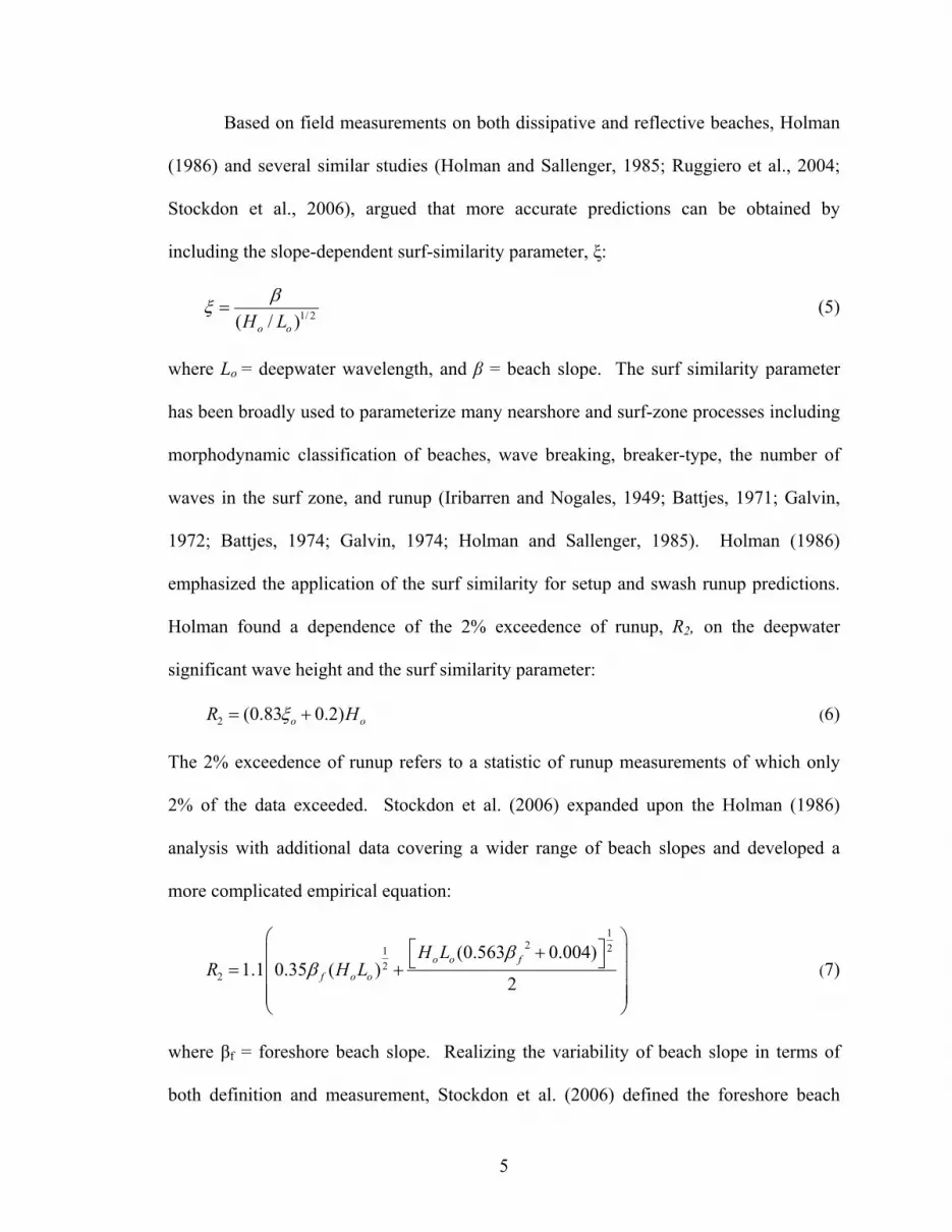
understood. Figure 1 illustrates the power density spectra of spilling and plunging

breakers measured during the LSTF experiments at an offshore gauge and at a gauge near

the shoreline. Most of the energy peaks within the high-frequency domain prior to wave

7

breaking. However, as the waves propagate onshore after breaking, much of the energy

peaks in the low-frequency domain. Although the significance of infragravity motions is

qualitatively recognized, existing theoretical and the empirical equations do not include

infragravity wave parameters.

Offshore (before breaking)

0.000

0.050

0.100

0.150

0.200

0.250

0.300

0.350

0.00 0.30 0.60 0.90 1.20 1.50Frequency (Hz)

Pow

er D

ensi

ty (m

^2 s

)

Spilling Plunging

Shoreline (after breaking)

0.000

0.010

0.020

0.030

0.040

0.050

0.060

0.070

0.080

0.090

0.00 0.30 0.60 0.90 1.20 1.50Frequency (Hz)

Pow

er D

ensi

ty (m

^2 s

)

Spilling Plunging

Figure 1. Power density spectra from the LSTF experiment under spilling and plunging breakers measured from an offshore gauge (above) and a gauge at the shoreline (below).

8

The definition of dissipative and reflective beaches was developed as a

classification scheme for overall beach morphology (Short, 1979a, b; Wright et al, 1979a,

b; Wright and Short, 1984). One of the key factors to the morphological classification is

beach slope (Fig. 2). However, the region over which beach slope is taken has an

influence on the value obtained, and therefore the classification of the beach. For

example, according to Wright and Short (1984), a dissipative beach is classified based on

tan β = 0.03 within the swash zone, and tan β = 0.01 across the inshore profile, or

nearshore region (Fig. 1). A reflective beach is defined as one with tan β = 0.1 to 0.2

within the swash zone, and tan β = 0.01 to 0.02 across the inshore profile (Fig. 2).

However, Nielsen and Hanslow (1991) suggested that the distinction between dissipative

or reflective should be tan β = 0.10. The method of determining slope was not specified.

The presence of an offshore bar and trough, a ridge-runnel system, rip channels or beach

cusps, etc., would result in an intermediate beach type between dissipative and reflective.

Therefore, based on Wright and Short (1984), many beaches fall within the intermediate

category. In addition, beach types can change with time, e.g., during calm and storm

conditions, and at different tidal stages. Holman and Sallenger (1985) suggested that

sometimes a beach can be considered as reflective during high tide and intermediate

during low tide due to the different intensity of bar influence on wave breaking.

In contrast to the importance of beach slope for determining the morphodynamic

classification of beaches and its influence on hydrodynamics, Douglass (1992) suggests

the slope term should not be used for the formulation of runup. After an analysis of the

effectiveness of including slope for estimating runup on beaches using Holman (1986)

data, Douglass found the prediction of runup was just as accurate with the omission of the

9

slope term. He also suggested that because the slope is a dependent variable and varies

significantly over time, determining its value a priori is difficult and unnecessary.

Figure 2. Beach-type classification based on beach morphology and slope (Wright and Short, 1984).

10

Almost all the above field studies focused mainly on the hydrodynamics of wave

runup with little discussion of the corresponding morphologic response, particularly the

upper limit of beach changes, which should be closely related to the wave runup. In

contrast to numerous studies on wave runup itself, limited data are available relating

wave runup excursion with the resulting morphologic change. In other words, it is not

well-documented how the limit of wave runup is related to the limit of beach change.

In the present study, data from the prototype-scale laboratory experiments,

including those conducted at SUPERTANK (Kraus et al., 1992; Kraus and Smith, 1994)

and the Large-Scale Sediment Transport Facility (LSTF) (Hamilton et al., 2001; Wang et

al., 2002), are analyzed to quantify the limit of wave runup and corresponding limit of

beach and dune erosion. Specifically, this study examines 1) the levels of swash run-up

and wave setup; 2) time-series beach-profile changes under erosional and accretionary

waves; 3) the relationship between the above two phenomena; and 4) the accuracy of

existing wave runup prediction methods. A new empirical formula predicting the limits

of wave runup based on breaking wave height, which also infers upper limit of beach

change, is based on the prototype-scale laboratory data. The formula predicting

maximum wave runup is Rmax=Hb. This first-order estimate has the advantage of giving

zero runup for zero wave height, in a much simpler form than many existing predictive

formulas.

11

Methods

SUPERTANK and LSTF Experiments

Data from two large-scale movable-bed laboratory studies, SUPERTANK and

LSTF experiments (Fig. 3), are examined to quantify the upper limits of beach-profile

change and wave runup, as well as to determine the relationship between the two. Both

experiments were specifically designed to measure detailed processes of sediment

transport and morphological change under varying prototype wave conditions. Dense

instrumentation in the well-controlled laboratory setting allows for the detailed and

accurate measurements of hydrodynamic conditions and time-series morphological

changes. In addition, large-scale physical analog models such as SUPERTANK and

LSTF are particularly useful in directly applying the same conditions to the real-world,

without the need for scaling. SUPERTANK was conducted in a two-dimensional wave

channel with beach changes caused primarily by cross-shore processes. LSTF is a three-

dimensional wave basin, with both cross-shore and longshore sediment transport

inducing beach change.

SUPERTANK is a multi-institutional effort sponsored by the U.S. Army Corps of

Engineers, conducted at the O.H. Hinsdale Wave Research Laboratory at Oregon State

University from July 29 to September 20, 1991. This facility is the largest wave channel

in the United States containing a sandy beach having the capability of running

12

experiments comparable to the magnitude of naturally occurring waves (Kraus et al.

1992). The SUPERTANK experiment measured total-channel hydrodynamics and

sediment transport along with resulting beach-profile changes. The wave channel is 104

m long, 3.7 m wide, and 4.6 m deep (with the still water level typically 1.5 m below the

top) with a constructed sandy beach extending 76 m offshore (Fig. 3 upper).

Figure 3. The SUPERTANK experiment (upper) and LSTF (lower) during wave runs.

LSTF

13

The beach was composed of 600 m3 of fine, well-sorted quartz sand with a

median size of 2.2 x 10-3 m and a fall speed of 3.3 x 10-2 m/s. The wave generator and

wave channel were equipped with a sensor to absorb the energy of waves reflected from

the beach (Kraus and Smith, 1994). The water-level fluctuations were measured with 16

resistance and 10 capacitance gauges. The 16 resistance gauges recorded water levels

and were mounted on the channel wall, spaced 3.7 m apart, extending from near the wave

generator to a water depth of approximately 0.5 m. The 10 vertical capacitance wave

gauges recording wave transformation and runup were mobile with spacing varying from

0.6 to 1.8 m, and extended from the most shoreward resistance gauge to the maximum

runup limit, sometimes submerged or partially buried. The 26 gauges provided detailed

wave propagation patterns, especially in the swash zone.

The beach profile was surveyed following each 20- to 60-min wave simulation.

The initial profile was constructed based on the equilibrium beach profile developed by

Dean (1977) and Bruun (1954) as:

23( )h x Ax= (8)

where h = still-water depth, x = horizontal distance from the shoreline, and A = a shape

parameter corresponding to a mean grain size of 3.0 x 10-3 m. The profile shape

parameter “A” varies with both sediment grain size and fall velocity, carrying dimensions

of length to the 1/3 power. The initial beach was built steeper with a greater A-value to

ensure adequate water depth in the offshore area (Wang and Kraus, 2005). For

efficiency, most SUPERTANK tests were initiated with the final profile of the previous

simulation. Approximately 350 beach-profile surveys were made with an auto-tracking,

infrared Geodimeter targeting prism attached to a survey rod mounted on a carriage

14

pushed by researchers. Although three lines, two along the wave-channel wall and one in

the center, were surveyed, only the center line was examined in this study, as the surveys

showed good cross-tank uniformity. Wave-processing procedures are discussed in Kraus

and Smith (1994). To separate incident-band wave motion from low-frequency motion, a

non-recursive, low-pass filter was applied to the total wave record during spectral

analysis. The period cutoff for the filter was set to twice the peak period of the incident

waves.

The LSTF is a three-dimensional wave basin located at the U.S. Army Corps of

Engineers Coastal and Hydraulic Laboratory in Vicksburg, Mississippi. Details of the

design and test procedures are discussed in Hamilton et al. (2001). The LSTF was

designed to study longshore sediment transport (Wang et al., 2002). Similar to the

SUPERTANK experiments, the LSTF is capable of generating wave conditions

comparable to the naturally occurring wave heights and periods found along low-energy

coasts. The LSTF has effective beach dimensions of 30-m cross-shore, 50-m longshore,

and walls 1.4 m high (Fig. 3 lower). The beach was typically designed in a trapezoidal

plan shape composed of approximately 150 m3 of very well-sorted fine quartz sand with a

median grain size of 1.5 x 10-3 m and a fall speed of 1.8 x 10-2 m/s. Initial construction of

the beach was also based on the equilibrium shape (Eq. 8). The beach profiles were

surveyed using an automated bottom-tracking profiler capable of resolving bed ripples.

The profiles surveyed in the center of the test basin are used here. The beach was

typically replenished after three to nine hours of wave activity. Long-crested and

unidirectional irregular waves with a relatively broad spectral shape were generated at a

10 degree incident angle. The wave height and peak wave period were measured with

15

capacitance wave gauges sampling at 20 Hz, with statistical wave properties calculated

by spectral analysis. The experimental procedures in LSTF are described in Wang et al.

(2002).

Data Analysis

After inspection of all 20 SUPERTANK tests, 5 tests with a total of 30 wave

simulations, or wave runs, were selected for analysis in the present study. The selection

was based on the particular purpose of the wave run, the trend of net sediment transport,

and measured beach change. Time-series beach-profile changes and cross-shore

distribution of wave height and mean water level were analyzed. During the 20 tests run

during the SUPERTANK experiment, approximately 350 beach-profile surveys were

conducted. For each profile, the elevation relative to mean water depth was plotted on

the vertical y-axis in meters and the distance offshore on the horizontal x-axis in meters.

The upper limits (UL) for the beach profile cases were identified based on the upper

profile convergence point, above which no beach change occurred.

The other location of importance along the profile was the lower limit of beach

change, sometimes referred to as the depth of closure. The lower limit, or profile

convergence point, was identified at the depth contour below which no beach-profile

change occurred. The depth of closure for a given or characteristic time interval is the

most landward depth seaward of which there is no significant change in bottom elevation

and no significant net sediment exchange between the nearshore and the offshore (Kraus,

et al., 1999; Wang and Davis, 1999).

16

For all 20 SUPERTANK cases examined, the water levels and zero-moment wave

heights were analyzed, where the mean water level or wave height (y-axis) was plotted

against the horizontal distance offshore (x-axis), respectively. The maximum runup (Rmax)

was defined by the location and beach elevation of the swash gauge that contained a

value larger than zero wave height, i.e., water reached that particular gauge. It is

important to note that the value of Rmax is not a statistical value, but rather an actual

measurement from the experiment. There may be some differences in the runup

measured in this study as compared to the video method (e.g., Holland et al., 1995) and

horizontally elevated wires (e.g., Guza and Thornton, 1982); however, because of the

finite spacing of the capacitance wave gauges in the swash zone, the differences are not

expected to be significant. Field measurements of wave runup have typically been

conducted with video imagery and/or resistance wire generally 5 to 20 cm above and

parallel to the beach face. Holman and Guza (1984) and Holland et al. (1995) compared

these two data collection methods concluding that they are comparable in producing

accurate results.

Cross-shore distribution of wave heights, or wave-energy decay, was also

examined. The wave breaker point was defined at the location with a sharp decrease in

wave height (Wang et al., 2002). Although the entire SUPERTANK dataset was

available for this study and were analyzed, 5 cases were selected from the 20 initial test

runs. The selection was based on the particular purpose of the wave run, the trend of net

sediment transport, and measured beach change.

Two LSTF experiments, one conducted under a spilling breaker and one under a

plunging breaker, are examined in this study. The LSTF analysis focused mainly on the

17

upper limit of beach change. The maximum runup was not directly measured due to the

lack of swash gauges. The main objective of the LSTF analysis was to apply the

SUPERTANK result to a three-dimensional beach.

The dataset from Holman (1986) was digitized. Similar statistical analysis, i.e.,

data normalization and linear regression analysis, were conducted to evaluate the

“goodness-of-fit” between the predicted and measured runup. In addition, polynomial

and exponential regression analyses were also conducted to examine potential non-linear

relationships between the measured wave runup and various parameters, such as wave

height, wave period, and beach slope.

18

Results

Overall, 30 SUPERTANK wave runs and two LSTF wave runs were analyzed

(Table 1). The thirty SUPERTANK cases were composed of twelve erosional random

wave runs, three erosional monochromatic wave runs, seven accretionary random wave

runs, three accretionary monochromatic wave runs, and five dune erosion random wave

runs, summarized in Table 1. The first two numbers in the Wave Run ID “10A_60ER”

indicate the major data collection test, the letter “A” (arbitrary nomenclature) indicates a

particular wave condition, and “60” describes the minutes of wave action. In design of

the experiment (Kraus et al., 1992) the erosional and accretionary cases were designed

based on the Dean number N,

bsHNwT

= (9)

where Hbs = significant breaking wave height; w = fall speed of the sediment, and T =

wave period.

Because the SUPERTANK experiments were designed to examine the processes-

response at a general beach-dune environment, rather than simulating a particular realistic

setting, e.g., a certain storm at a certain beach, scaling is not a particular concern. Of

course, caution should be taken when applying the SUPERTANK findings to different

conditions in the real world. However, this holds true when applying findings of any

19

field experiment, e.g., from the Pacific coasts to the Gulf of Mexico coasts, from one

setting to another.

Table 1. Summary of Selected Wave Runs and Input Wave and Beach Conditions (Notation is explained at the bottom of the table).

Wave Run ID

Ho m

Tp s

Lo m n N

Hbs m βs

ξ Hb_h

m Hb_l m

Hsl_h m

Hsl_l m

SUPERTANK 10A_60ER 0.78 3.0 14.0 20 6.4 0.68 0.10 0.42 0.66 0.15 0.13 0.24 10A_130ER 0.78 3.0 14.0 20 6.8 0.68 0.09 0.38 0.67 0.15 0.10 0.23 10A_270ER 0.78 3.0 14.0 20 6.9 0.68 0.10 0.42 0.65 0.16 0.10 0.24 10B_20ER 0.71 3.0 14.0 3.3 6.6 0.65 0.14 0.58 0.63 0.17 0.10 0.23 10B_60ER 0.73 3.0 14.0 3.3 6.8 0.67 0.11 0.44 0.65 0.17 0.11 0.24 10B_130ER 0.72 3.0 14.0 3.3 7.0 0.69 0.09 0.36 0.67 0.18 0.12 0.25 10E_130ER 0.69 4.5 31.6 20 4.9 0.72 0.11 0.69 0.71 0.15 0.15 0.16 10E_200ER 0.69 4.5 31.6 20 5.0 0.74 0.12 0.77 0.72 0.15 0.15 0.18 10E_270ER 0.69 4.5 31.6 20 5.1 0.76 0.09 0.58 0.74 0.15 0.16 0.20 10F_110ER 0.66 4.5 31.6 3.3 5.1 0.75 0.09 0.58 0.72 0.18 0.15 0.26 10F_130ER 0.68 4.5 31.6 3.3 5.1 0.76 0.08 0.48 0.74 0.18 0.13 0.21 10F_170ER 0.69 4.5 31.6 3.3 5.1 0.76 0.08 0.50 0.73 0.20 0.12 0.24 G0_60EM 1.05 3.0 14.0 M 10.0 1.18 0.10 0.43 1.18 0.01 0.11 0.03 G0_140EM 1.04 3.0 14.0 M 10.5 1.04 0.10 0.41 1.04 0.04 0.08 0.10 G0_210EM 1.15 3.0 14.0 M 10.8 1.07 0.09 0.39 1.07 0.04 0.11 0.02 30A_60AR 0.34 8.0 99.9 3.3 1.6 0.41 0.14 2.24 0.40 0.06 0.24 0.08 30A_130AR 0.33 8.0 99.9 3.3 1.6 0.39 0.13 2.09 0.38 0.06 0.24 0.09 30A_200AR 0.34 8.0 99.9 3.3 1.6 0.41 0.13 2.02 0.40 0.06 0.25 0.10 30C_130AR 0.31 9.0 126.4 20 1.4 0.40 0.13 2.36 0.40 0.04 0.18 0.05 30C_200AR 0.31 9.0 126.4 20 1.4 0.39 0.15 2.31 0.38 0.04 0.19 0.06 30C_270AR 0.31 9.0 126.4 20 1.4 0.39 0.15 2.60 0.38 0.04 0.20 0.06 30D_40AR 0.37 9.0 126.4 20 1.4 0.42 0.13 2.00 0.42 0.05 0.17 0.07 I0_80AM 0.60 8.0 99.9 M 2.9 0.76 0.20 2.78 0.76 0.01 0.38 0.03 I0_290AM 0.63 8.0 99.9 M 3.1 0.81 0.17 2.35 0.81 0.01 0.34 0.02 I0_590AM 0.60 8.0 99.9 M 2.7 0.72 0.12 1.64 0.73 0.01 0.25 0.03 60A_40DE 0.69 3.0 14.0 3.3 6.2 0.61 0.12 0.55 0.58 0.14 0.16 0.24 60A_60DE 0.69 3.0 14.0 3.3 6.2 0.61 0.10 0.46 0.60 0.14 0.12 0.24 60B_20DE 0.64 4.5 31.6 3.3 4.4 0.66 0.11 0.74 0.63 0.15 0.18 0.24 60B_40DE 0.63 4.5 31.6 3.3 4.4 0.66 0.11 0.76 0.62 0.16 0.18 0.25 60B_60DE 0.65 4.5 31.6 3.3 4.4 0.66 0.12 0.79 0.63 0.17 0.18 0.30 LSTF Spilling 0.27 1.5 3.5 3.3 10.0 0.26 0.11 0.41 N/C N/C N/C N/C Plunging 0.24 3.0 14.0 3.3 4.4 0.27 0.13 0.96 N/C N/C N/C N/C

ER = erosional random wave; EM = erosional monochromatic wave; AR = accretionary random wave; AM = accretionary monochromatic wave; DE = dune erosion case; Ho = offshore wave height; Tp = peak wave period; Lo = offshore wavelength; n = spectral peakness; N = Dean Number; Hbs = significant breaking wave height; βs. = beach slope defined as the slope of the section approximately 1 m landward and 1 m seaward of the shoreline; ξ = surf similarity parameter; Hb_h = incident band wave height at the breaker line; Hb_l = low frequency band wave height at the breaker line; Hsl_h = incident band wave height at the shoreline; Hsl_l = low-frequency band wave height at the shoreline; N/C = Not calculated.

20

Beach Profile Change

Typically, erosion is defined as a net offshore transport of sand resulting in a net

loss of beach volume above the mean water line, or shoreline. Accretion is defined as a

total net onshore transport of sand, building the beach above mean water level. These

definitions are applied in this study. For the SUPERTANK wave runs examined, the

Dean number N was typically between 5 and 10 for the erosional cases. For the

accretionary cases, the N was typically between 1.5 and 3 (Table 1). For the LSTF

experiment, the spilling breaker case had a Dean Number of 10, indicating a highly

erosive wave. A smaller Dean Number of 4.4 corresponds to the plunging breaker case,

indicative of a slightly more accretionary trend (Table 1).

The first SUPERTANK wave run, ST_10A, was conducted over the monotonic

initial profile (Eq. 8). Significant beach-profile change occurred with substantial

shoreline recession, along with the development of an offshore bar. Figure 4 illustrates

four time-series beach-profiles surveyed at initial, 60, 130, and 270 minutes. Initially, the

overall foreshore exhibited a convex shape while the end profile was concave. After 60

min of wave action, considerable erosion occurred in the vicinity of the shoreline. The

sand was transported offshore and deposited in the form of a bar. This trend continued

during the subsequent wave runs, with additional erosion near the shoreline and further

accretion of the bar with offshore directed migration. After 270 min, the bar had moved

4 m further offshore, compared to the 60-minute bar location. The 270-min profile was

substantially steeper near the shoreline than the initial profile. The maximum beach-face

recession occurred at the +0.37 m contour line. The morphology of a section of the beach

profile located landward of the trough (from 15 to 18 m) did not experience any changes,

21

indicating that the sediment eroded from near the shoreline was transported past this

section of the surf zone and deposited on the bar. The upper limit of beach-profile

change can be readily identified; for this case, the upper limit was 0.66 m above mean

water level (MWL) for all three time segments. There is also an apparent point of profile

convergence in the offshore area, at -1.35 m depth contour, beyond which regular profile

elevation change cannot be identified.

ST_10A: Equilibrium Erosion (Random)

-1.8

-1.2

-0.6

0.0

0.6

1.2

1.8

0 5 10 15 20 25 30 35Distance (m)

Elev

atio

n re

lativ

e to

MW

L (m

)

initial 60 min 130 min. 270 min.

Hmo = 0.8 mTp = 3 sn = 20

Figure 4. The first SUPERTANK wave run, ST_10A erosive case. Substantial shoreline erosion occurred on the initial monotonic profile with the development of an offshore bar. The horizontal axis “distance” refers to the SUPERTANK coordinate system and not directly related to morphological features.

22

The subsequent wave runs were conducted over the final profile of the previous

wave run, i.e., a barred beach. The beach-profile changes are detectable, but subtle,

especially for the accretionary wave cases with lower wave heights. Figure 5 shows an

example of an accretionary wave run, ST_30A. Overall, compared to the initial run (Fig.

3), the beach-profile changes were much more subtle. The top of the offshore bar was

eroded with sediment deposition along the landward slope of the bar (Fig. 5 upper). The

subtle profile change near the shoreline, viewed at a smaller scale (Fig. 5 lower),

indicates slight accretion. The accreted sand apparently came from the erosion just below

the MWL. Due to the slight change, the identification of the upper limit is more difficult

than the first case, and is less certain. This upper limit is determined to be at 0.31 m

above MWL (Fig. 5 lower). One of the surveys (60 min.) exhibits some changes above

that convergence level, however these changes have been interpreted as survey error.

The offshore-profile convergence point was determined to be located at a depth contour

of -1 m.

A scarp developed during some of the erosional wave runs (Fig. 6). The

development of the scarp is induced by waves eroding the base of the dune or the dry-

beach, subsequently causing the weight of the overlying sediment to become unstable and

collapse. The resulting beach slope immediately seaward of the scarp on the beach face

tends to be steeper than on a non-scarped beach. The upper limit of beach change is

apparently at the top of the scarp, controlled by the elevation of the beach berm or dune,

and does not necessarily represent the vertical extent of wave action. The nearly vertical

scarp also induces technical difficulties of measuring the runup using wire gages. The

upper limit of beach change in this study was selected at the base of the near-vertical

23

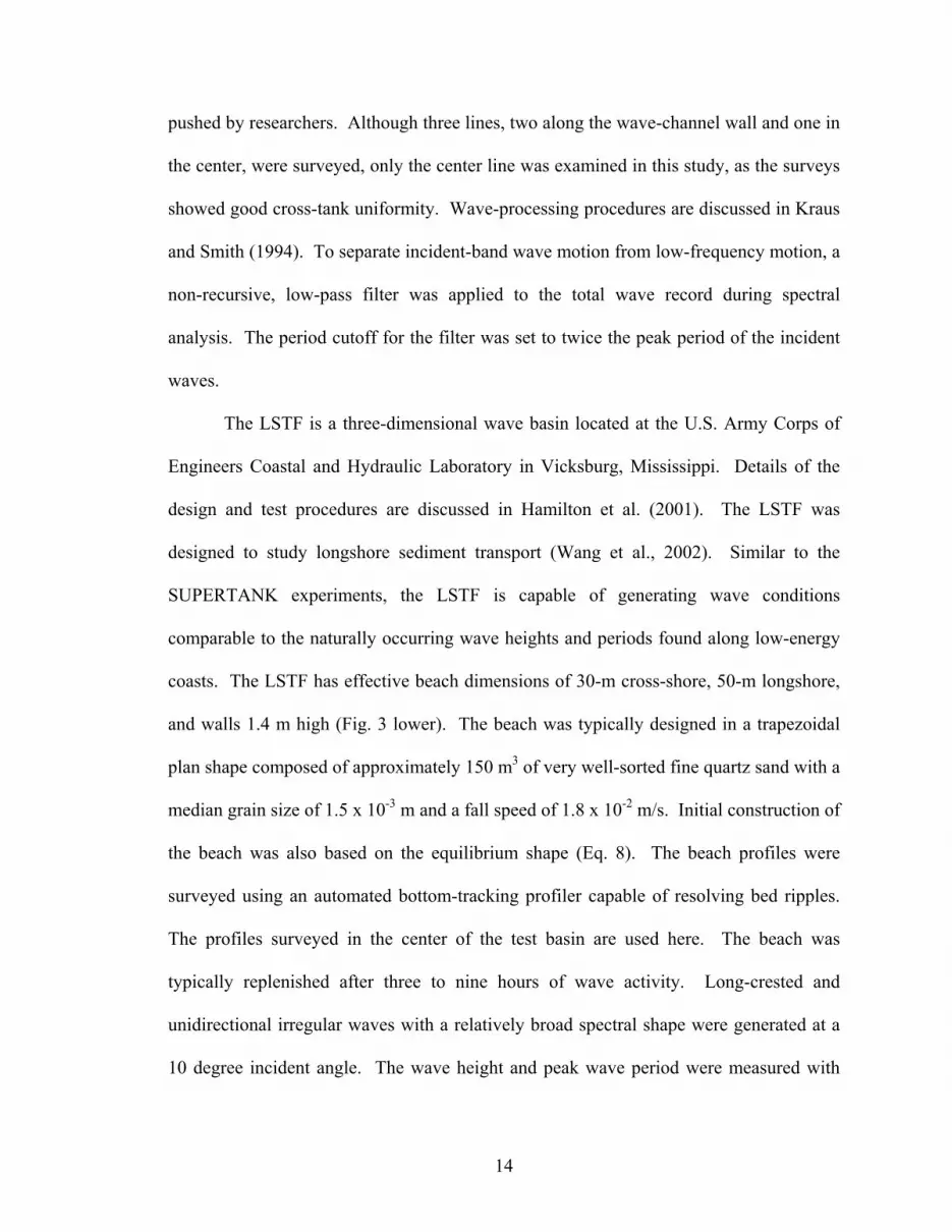
scarp, measured at 0.31 m above MWL during ST_60A (Fig. 6). The collapsed sediment

from the scarp was deposited just below MWL (40 and 60 min). Therefore, for the

scarped case, the upper limit is controlled by both wave action and gravity-driven

sediment collapsing. Few beach-profile changes were measured offshore.

SUPERTANK experiments also included several cases conducted under

monochromatic waves. Overall, beach-profile changes induced by monochromatic wave

action were substantially different from those under the more realistic random waves (Fig.

7). The monochromatic waves tended to create irregular and undulating profiles. For

ST_I0, the upper limit of beach-profile change was estimated at around 0.50 m and varied

slightly during different wave runs. A persistent onshore migration of the offshore bar

also occurred throughout the wave runs, with several secondary bars developed in the

mid-surf zone. The erratic profile evolution did not seem to approach a stable

equilibrium shape, and does not have an apparent profile convergence point. In addition,

it is important to note that the profile shape developed under monochromatic waves does

not represent profiles typically measured in the field (Wang and Davis, 1998). This

implies that morphological changes measured in movable-bed laboratory experiments

under monochromatic waves may not be applicable to real world conditions, despite the

easier hydrodynamic parameterization and analysis of monochromatic waves.

24

ST_30A: Equilibrium Accretion (Random)

-0.3

-0.2

-0.1

0.0

0.1

0.2

0.3

0.4

0.5

4 6 8 10Distance (m)

Elev

atio

n re

lativ

e to

MW

L (m

)

initial 60 min. 130 min. 200 min.

Hmo = 0.4 mTp = 8 sn = 3.3

Figure 5. The SUPERTANK ST_30A accretionary wave run. There was subtle shoreline accretion, with an onshore migration of the offshore bar (upper). The subtle accretion near the shoreline is identified when viewed at a smaller scale (lower).

ST_30A: Equilibrium Accretion (Random)

-1.8

-1.2

-0.6

0.0

0.6

1.2

1.8

0 5 10 15 20 25 30 35Distance (m)

Ele

vatio

n re

lativ

e to

MW

L (m

)

initial 60 min. 130 min. 200 min.

Hmo = 0.4 mTp = 8 sn = 3.3

25

ST_60A: Dune Erosion 2/2

-1.8

-1.2

-0.6

0.0

0.6

1.2

1.8

0 5 10 15 20 25 30 35Distance (m)

Elev

atio

n re

lativ

e to

MW

L (m

)

initial 40 min. 60 min.

Hmo = 0.7 mTp = 3 sn = 3.3

Figure 6. The SUPERTANK ST_60A dune erosion wave run. A nearly vertical scarp was developed after 40 minutes of wave action, with the upper limit of beach change identified at the toe of the dune-scarp.

Similar analyses as described above were also conducted to a set of three-

dimensional laboratory movable-bed experiments at LSTF. The waves generated in

LSTF had smaller wave heights as compared to the SUPERTANK waves. Two cases

with distinctively different breaker types, one spilling and one plunging, were examined

in this study. The beach profiles used in the following discussion are averaged over the

middle section of the wave basin, and therefore represent the average condition of the 3-

dimensional beach.

26

ST_I0: Equilibrium Accretion (Monochromatic)

-1.8

-1.2

-0.6

0.0

0.6

1.2

1.8

0 5 10 15 20 25 30 35Distance (m)

Elev

atio

n re

lativ

e to

MW

L (m

)

initial 80 min 290 min 590 min

Hmo = 0.5 mTp = 8 sMON

Figure 7. The SUPERTANK ST_I0 accretionary monochromatic wave run. The resulting beach-profile under monochromatic waves is erratic and undulating.

The spilling wave run was initiated with the Dean equilibrium beach profile.

Because of the smaller wave heights, the beach-profile changes occurred at a slower rate.

Similar to the first SUPERTANK wave run, ST_10A, a subtle bar formed over the initial

monotonic beach profile (Fig.8 upper). The upper limit of beach change was 0.23 m

above MWL under the spilling waves, as identified from the smaller scale plot (Fig. 8

lower). Sediment from the eroding foreshore was apparently transported seaward to the

offshore bar. As the foreshore eroded, the offshore bar accumulated sediment

increasingly with each subsequent wave run. Between 5 and 9 m offshore, little to no

27

change occurred which could suggest that the sediment bypassed this region and

terminated transport at the offshore bar. The profile converges on the seaward slope of

the offshore bar.

LSTF Spilling Wave Case

-0.05

0.00

0.05

0.10

0.15

0.20

0.25

0.30

0.35

-1.5 -1.2 -0.9 -0.6 -0.3 0

Distance (m)

Elev

atio

n re

lativ

e to

MW

L (m

)

0 min 510 min 890 min 1330 min

Hmo = 0.27 mTp = 1.5 sn = 3.3

Figure 8. The LSTF Spilling wave case. Erosion occurred in the foreshore and inner surf zone. The eroded sediment was deposited on an offshore bar.

LSTF Spilling Wave Case

-0.8

-0.6

-0.4

-0.2

0.0

0.2

0.4

-3 -2 -1 0 1 2 3 4 5 6 7 8 9 10 11 12 13 14 15 16

Distance (m)

Elev

atio

n re

lativ

e to

MW

L (m

)

0 min 510 min 890 min 1330 min

Hmo = 0.27 mTp = 1.5 sn = 3.3

28

For the plunging wave case at LSTF, shoreline advancement occurred with each

wave run along with a persistent onshore migration of the bar (Fig. 9 upper). This

corresponds to a lower Dean number of 4.4. The accumulation at the shoreline was

subtle, but can be identified when viewed at a smaller spatial scale (Fig. 9 lower). The

upper limit of beach-profile change is located at 0.26 m above MWL, with the lower limit

identified at the profile convergence point midway on the seaward slope of the bar. Also,

persistent erosion was measured just below the MWL and at a region landward of the

initial secondary bar. The eroded sediment landward of the trough may have contributed

to the onshore migration of the offshore bar (Fig. 9 upper). Overall, the trends observed

in the three-dimensional LSTF experiment were comparable to those in the two-

dimensional SUPERTANK experiment.

Table 2 summarizes the upper and lower limits of change during each wave run,

including the breaking wave height. Overall, for the 30 SUPERTANK wave runs and 2

LSTF wave runs, the incident breaking wave height ranged from 0.26 to 1.18 m (Table 2).

The measured upper limit of profile change, including the scarped cases, ranged from

0.23 to 0.70 m. The lower limit of beach change ranged from 0.50 to 1.61 m below

MWL. Relationships between the profile changes and wave conditions are discussed in

the following sections.

29

LSTF Plunging Wave Case

0.14

0.16

0.18

0.20

0.22

0.24

0.26

0.28

0.30

0.32

0.34

-1.8 -1.7 -1.6 -1.5 -1.4 -1.3 -1.2 -1.1 -1Distance (m)

Elev

atio

n re

lativ

e to

MW

L (m

)

pre-test 40 min 80 130

Hmo = 0.24 mTp = 3 sn = 3.3

Figure 9. The LSTF Plunging wave case. Slight foreshore accretion and landward migration of the offshore bar occurred during the wave run.

LSTF Plunging Wave Case

-0.8

-0.6

-0.4

-0.2

0.0

0.2

0.4

-3 -2 -1 0 1 2 3 4 5 6 7 8 9 10 11 12 13 14 15 16Distance(m)

Ele

vatio

n re

lativ

e to

MW

L (m

)

pre-test 40 min 80 130

Hmo = 0.24 mTp = 3 sn = 3.3

30

Table 2. Summary of Breaking Wave, Maximum Wave Runup, Upper and Lower limits of Beach-Profile Changes, and Presence of a Scarp for Each Analyzed Wave Run.

Wave Run Hb Rmax UL LL Scarp ID m m m m SUPERTANK 10A_60ER 0.68 0.6 0.66 1.29 No 10A_130ER 0.68 0.6 0.66 1.29 No 10A_270ER 0.68 0.7 0.66 1.29 No 10B_20ER 0.65 0.33 0.67 1.35 No 10B_60ER 0.67 0.69 0.67 1.35 No 10B_130ER 0.69 0.64 0.67 1.35 No 10E_130ER 0.72 0.3 0.74 1.52 No 10E_200ER 0.74 0.78 0.84 1.52 No 10E_270ER 0.76 0.45 0.84 1.52 No 10F_110ER 0.75 0.38 0.43 1.52 Yes 10F_130ER 0.76 0.38 0.42 1.52 Yes 10F_170ER 0.76 0.38 0.48 1.52 Yes G0_60EM 1.18 0.28 0.38 1.61 No G0_140EM 1.04 0.18 0.25 1.61 Yes G0_210EM 1.07 0.32 0.27 1.61 Yes 30A_60AR 0.41 0.42 0.31 1.36 No 30A_130AR 0.39 0.42 0.31 1.36 No 30A_200AR 0.41 0.42 0.31 1.36 No 30C_130AR 0.4 0.41 0.39 1.01 No 30C_200AR 0.39 0.42 0.42 1.01 No 30C_270AR 0.39 0.42 0.42 1.01 No 30D_40AR 0.42 0.23 0.43 0.65 No I0_80AM 0.76 0.27 0.46 1.82 No I0_290AM 0.81 0.16 0.53 1.82 No I0_590AM 0.72 0.35 0.53 1.82 Yes 60A_40DE 0.61 0.17 0.28 1.16 Yes 60A_60DE 0.61 0.17 0.28 1.16 Yes 60B_20DE 0.66 0.16 0.38 0.99 Yes 60B_40DE 0.66 0.16 0.38 0.99 Yes 60B_60DE 0.66 0.17 0.38 0.99 yes LSTF Spilling 0.26 N/M 0.23 0.62 No Plunging 0.27 N/M 0.26 0.5 No

Hb = breaker height measured; Rmax= maximum runup measured (not statistical); UL, LL = upper and lower limit of beach change, respectively; NM = not measured.

31

Cross-shore Distribution of Wave Height

The wave-height decay is representative of the wave-energy dissipation as a wave

propagates onshore. Detailed wave decay patterns were measured by the closely spaced

wave gauges for both SUPERTANK and LSTF experiments. Figure 10 shows time-

series wave decay patterns measured at the first SUPERTANK wave run, ST_10A. As

discussed earlier, considerable beach profile change, for example the formation of an

offshore bar, was measured during this wave run (Fig. 4). The substantial morphology

change also influenced the pattern of wave decay.

ST_10A

0.0

0.1

0.2

0.3

0.4

0.5

0.6

0.7

0.8

0.9

0 10 20 30 40 50 60 70 80Distance (m)

Hm

o (m

)

60 min. 130 min. 270 min.

Figure 10. The cross-shore random wave-height distribution measured during SUPERTANK ST_10A; yellow arrow indicates the breaker point.

32

The inflection point of wave decay migrated slightly as the beach morphology

changed from the initial monotonic profile to a barred-beach profile. This point is

defined as the location and height at which the wave breaks (Wang et al., 2002). For

ST_10A, the significant breaking wave height is 0.68 m. The rate of wave-height decay

tends to be smaller in the mid-surf zone (10 to 20 m) as compared to the breaker zone (20

to 25 m) and the inner surf zone (landward of 10 m). The offshore wave height remains

largely constant until reaching the breaker line.

The wave decay pattern for the longer period accretionary wave case, ST_30A (Fig.

11), was considerably different than the steep erosive waves. The significant breaking

wave height was 0.36 m. The time-series wave pattern remained constant for each wave

run, apparently not influenced by the subtle morphology change (Fig.5). The offshore

bar formed at 30 m during the previous experiment with higher wave heights. Instead of

wave breaking over the bar, shoaling of the long period wave was measured (at around 30

m). The main breaker line is identified at around 20 m.

33

ST_30A

0.0

0.1

0.2

0.3

0.4

0.5

0 10 20 30 40 50 60 70 80Distance (m)

Hm

o (m

)

60 min. 130 min. 200 min.

Figure 11. The cross-shore random wave-height distribution measured during SUPERTANK ST_30A.

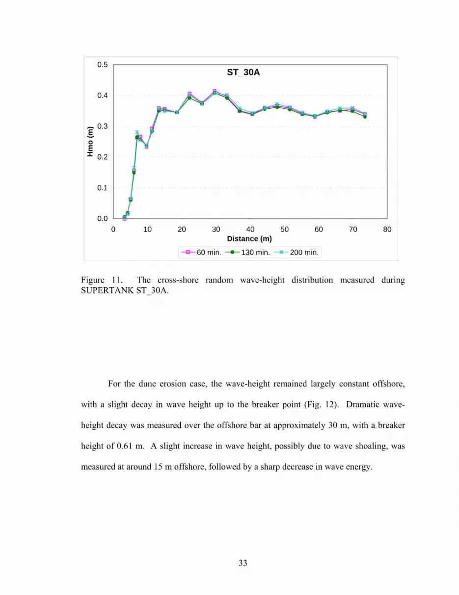
For the dune erosion case, the wave-height remained largely constant offshore,

with a slight decay in wave height up to the breaker point (Fig. 12). Dramatic wave-

height decay was measured over the offshore bar at approximately 30 m, with a breaker

height of 0.61 m. A slight increase in wave height, possibly due to wave shoaling, was

measured at around 15 m offshore, followed by a sharp decrease in wave energy.

34

ST_60A

0.0

0.1

0.2

0.3

0.4

0.5

0.6

0.7

0.8

0 10 20 30 40 50 60 70 80Distance (m)

Hm

o (m

)

40 min. 60 min.

Figure 12. The cross-shore random wave-height distribution measured during SUPERTANK ST_60A.

The cross-shore distribution of wave heights for the monochromatic wave case

ST_I0 was rather erratic with both temporal and spatial inconsistencies (Fig. 13). This

corresponds to the irregular beach-profile change observed during this wave case (Fig. 7).

The breaking wave height varied considerably, from 0.72 to 0.81 m. The wave-height

variation in the offshore region, seaward of the breaker line around 30 m, is probably

related to oscillations in the wave tank. However, the irregular breaking wave heights

were likely caused by reflection of the regular waves off the beach face.

35

ST_I0

0.0

0.1

0.2

0.3

0.4

0.5

0.6

0.7

0.8

0.9

0 10 20 30 40 50 60 70 80Distance (m)

Hm

o (m

)

80 min. 290 min. 590 min.

Figure 13. The cross-shore monochromatic wave-height distribution measured during SUPERTANK ST_I0.

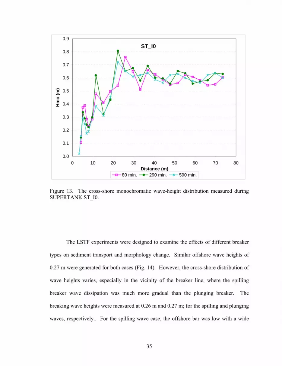
The LSTF experiments were designed to examine the effects of different breaker

types on sediment transport and morphology change. Similar offshore wave heights of

0.27 m were generated for both cases (Fig. 14). However, the cross-shore distribution of

wave heights varies, especially in the vicinity of the breaker line, where the spilling

breaker wave dissipation was much more gradual than the plunging breaker. The

breaking wave heights were measured at 0.26 m and 0.27 m; for the spilling and plunging

waves, respectively.. For the spilling wave case, the offshore bar was low with a wide

36

crest at around 12 m offshore (Fig. 9) with the main breaker line just seaward of the bar

crest (Fig. 14). The narrow bar during the plunging case migrated onshore from 13 to 11

m (Fig. 9), with the main breaker line occurring directly over the crest of this bar (Fig.

14). Again, the wave height decay at the breaker line was more abrupt for the plunging

case than for the spilling case, as expected.

Spilling and Plunging

0.00

0.05

0.10

0.15

0.20

0.25

0.30

0.35

0 2 4 6 8 10 12 14 16 18Distance (m)

Hm

o (m

)

Spilling Plunging

Figure 14. The cross-shore wave-height distribution and γ for the LSTF Spilling and Plunging wave cases.

37

Wave Runup

The extent and elevation of wave runup for the SUPERTANK experiments were

measured directly by the closely spaced swash gages (Kraus and Smith, 1994). Figure 15

shows the cross-shore distribution of time-averaged water level for the erosive wave run,

ST_10A. As expected, the mean water level in the offshore area remained largely at zero.

Elevated water levels were measured in the surf zone. It is important to separate the

elevation caused by wave setup and swash runup, although it is often difficult to do.

Currently, there is no widely accepted method for separating the setup from the swash in

total wave runup. In this study, the elevated water levels seaward and landward of the

still-water shoreline are regarded as wave setup and swash runup, respectively. This

convention coincides well with the inflection point of the change in slope of the cross-

shore distribution of the mean water level (Fig. 15). The setup approaches the shoreline

asymptotically following the slope or curvature of the beach face, whereas the swash

appears to be nearly vertical controlled by the gauge elevation. For this case, the setup

measured at the still-water shoreline was 0.1 m, which is about 17 percent of the total

wave runup of 0.6 m, consistent with the approximation for setup by Guza and Thornton

(1982). The slight difference in wave runup among different wave runs was attributed to

the considerable beach-profile change during the first SUPERTANK wave case.

38

ST_10A

-0.2-0.1

00.10.20.30.40.50.60.70.8

0 10 20 30 40 50 60 70 80Distance (m)

Mea

n W

ater

Lev

el (m

)

60 130 270

Figure 15. Wave runup measured during SUPERTANK ST_10A.

For the accretionary wave case, ST_30A, the curvature in the mean-water level

also coincides with the still-water shoreline (Fig. 16). However, considerable variations

in the wave setup occurred at the shoreline. The slight decrease in mean water level

measured just seaward of 20 m offshore during the 130-min wave run is attributed to

setdown. The increase measured just seaward of 20 m offshore during the 270-min wave

run is likely caused by instrument error at that particular location. The average setup at

the shoreline was approximately 0.07 m, also about 17 percent of the total measured

wave runup of 0.42m.

39

ST_30A

-0.050

0.050.1

0.150.2

0.250.3

0.350.4

0.450.5

0 10 20 30 40 50 60 70 80Distance (m)

Mea

n W

ater

Lev

el (m

)

60 130 200

Figure 16. Wave runup measured during SUPERTANK ST_30A.

Total wave runup was significantly limited by the vertical scarp as shown in the

dune erosion case of ST_60A (Fig. 17). A broad set down was measured just seaward of

the main breaker line. The curvature of the cross-shore distribution of the mean water

level occurred between 10 and 11 m, which was different from the still-water shoreline at

8 m. The setup measured at the water-level curvature at 11 m was approximately 0.03 m.

Despite the limited total runup, the wave setup contributes 18 percent of the total wave

runup of 0.17 m, similar to the above two cases.

The cross-shore distribution of time-averaged mean water levels for ST_I0 were

somewhat erratic (Fig. 18), similar to the erratic beach-profile changes and cross-shore

distribution of wave heights for the monochromatic wave runs. Different from the

irregular wave cases, a zero mean-water level was not measured at a several offshore

wave gauges.

40

ST_60A

-0.04-0.02

00.020.040.060.080.1

0.120.140.160.18

0 20 40 60 80Distance (m)

Mea

n W

ater

Lev

el (m

)

40 60

Figure 17. Wave runup measured during SUPERTANK ST_60A.

ST_I0

-0.1

-0.05

0

0.05

0.1

0.15

0.2

0.25

0.3

0.35

0.4

0 10 20 30 40 50 60 70 80Distance (m)

Mea

n W

ater

Lev

el (m

)

80 290 590

Figure 18. Wave runup measured during SUPERTANK ST_I0.

41

In addition, considerable variances among different wave runs were also measured.

The total wave runup varied from 0.16 to 0.35 m, with an average of 0.26 m. The

curvature in the mean-water level distribution coincides with the still-water shoreline at 5

m. The maximum setup at the still-water shoreline was 0.08 m, which is 31 percent of

the total wave runup. The lesser contribution of the swash runup to the total wave runup

can be attributed to the lack of low-frequency motion in the monochromatic waves,

exemplified in Table 1, in which the low- frequency components of the swash (Hsl_l) for

monochromatic waves were much smaller than the contribution for random waves.

42

Discussion

Relationship between Wave Runup, Incident Wave Conditions, and Limit of Beach Profile Change

The measured breaking wave height, upper limit of beach-profile change, and

wave runup from the SUPERTANK experiments are compared in Figure 19. The thirty

cases examined are divided into three categories, including non-scarped random wave

runs, scarped random wave runs, and monochromatic wave runs. The upper limit of

beach change was almost equal to the maximum excursion of wave runup for the non-

scarped cases. In addition, the maximum wave runup was nearly equal to the breaking

wave height for the non-scarped random wave cases as well. This suggests that the

breaking wave height is equal to the maximum elevation of wave runup which is equal to

the upper limit of beach change, emphasized by the 16 non-scarped random wave runs,

except the three cases 10B_20ER, 10E_270ER and 30D_40AR. The cause of the

discrepancy in the data for these outliers varies. During the SUPERTANK experiment, it

was confirmed that the capacitance gauges could record the wet sand or water surface if

the sand was fully saturated. Some degradation in the response was found if the sand was

not fully saturated, which could explain the limited swash runup measurement during the

first 20 min run of ST10B. However, a direct cause for the other two questionable

measurements is not clear.

43

0

0.2

0.4

0.6

0.8

1

1.2

1.410

A_6

0ER

10A

_270

ER

10B

_60E

R

10E

_130

ER

10E

_270

ER

30A

_130

AR

30C

_130

AR

30C

_270

AR

10F_

130E

R

60A

_40D

E

60B

_20D

E

60B

_60D

E

G0_

60E

M

G0_

210E

M

I0_2

90A

M

Wave Run No.

Upp

er L

imit

(m)

Breaking Wave Height Beach Change Wave Runup

Non-scarped Random Wave Cases Scarped Random Wave Cases

Monochromatic Wave Cases

Figure 19. Relationship between breaking wave height, upper limit of beach profile change, and wave runup for the thirty SUPERTANK cases examined.

Based on the criteria of identifying the upper limit of beach change at the toe of

the scarp, for the scarped random wave cases the breaking wave height was much higher

than the elevation of wave runup, which was limited by the vertical scarp. The definition

was based on the fact that any change occurring above this point was likely due to the

weight of the overlying sediment collapsing. The true upper limit of change is thus

controlled by the elevation of the beach or dune. No relationship among the breaker

height, wave runup, and beach-profile change was found for the scarped random wave

44

runs. However, it is important to note that the upper limits of beach changes for scarped

cases are not expected to relate to wave runup.

The much lower wave runup under monochromatic waves as compared to the

breaker height was found to be caused by the lack of low-frequency motion. Baldock and

Holmes (1999) suggested that simulating irregular waves with overlapping

monochromatic swash events could reproduce both low and high frequency spectral

characteristics of the swash zone. No SUPERTANK experiments were designed to

investigate this. No relationship could be found among the above three factors for

monochromatic waves. This further suggests that despite the convenience associated

with studying the hydrodynamics associated with regular waves, including

monochromatic waves in laboratory experiments related to morphology changes, they do

not have direct real-world applications.

Based on the above observations from the SUPERTANK data (Fig. 19), a direct

relationship between the measured runup height on a non-scarp beach and the breaker

height is proposed:

max bsR H= (10)

The average ratio of Rmax over Hbs for the 16 non-scarped wave cases was 0.93 with a

standard error on the mean of 0.05. Excluding the three outliers, 10B_20ER, 10E_270ER

and 30D_40AR, the average Rmax/Hbs was 1.01 with a standard error of 0.02. To be

conservative due to the limited data coverage, a value of one is used in Eq. (10). In

addition, the maximum runup elevation for the non-scarped random wave cases was

approximately equal to the upper limit of beach change,

LUR =max (11)

45

This is important for relating morphological changes to wave runup on beaches, which is

a main goal of runup studies. However, this relationship is most directly applied to wave

similar to those generated in the two physical analog models. In addition, a wider range

of runup and significant wave heights would likely increase the reliability of the

correlation coefficient.

Therefore, it is suggested that the breaker height is equal to the upper limit of

wave runup which is equal to the upper limit of beach changes,

Lbs URH == max (12)

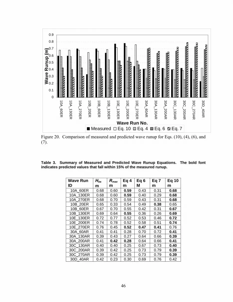
Comparisons of the measured wave runup with the various existing empirical

formulas (Eqs. 4, 6, and 7) and the new model (Eq. 10) are summarized in Figure 20 and

Table 3. As shown in Fig. 20, the simple new model reproduced the measured wave

runup much closer than the other formulas. For the 16 non-scarped SUPERTANK wave

cases, 81% of the predictions from Eq. (10) fall within 15% of the measured wave runup.

In contrast, for Eqs. (4), (6) and (7), only 25%, 6% and 13% of the predictions,

respectively fall within 15% of the measured values. Eqs. (6) and (7) under-predicted the

measured wave runup for the erosional cases and over-predicted runup for the

accretionary wave cases. The loss of predictive capability is caused by the substantially

greater ξ for the gentle long-period accretionary waves than for the steep short-period

erosional waves (Table 1). Agreement between measured and predicted values was

actually reduced by including the surf similarity parameter, ξ. The simpler Eq. (4), using

just offshore wave height, more accurately reproduced the measured values of wave

runup than Eqs. (6) and (7).

46

0

0.1

0.2

0.3

0.4

0.5

0.6

0.7

0.8

0.9

10A_60E

R

10A_130E

R

10A_270E

R

10B_20E

R

10B_60E

R

10B_130E

R

10E_130E

R

10E_200E

R

10E_270E

R

30A_60A

R

30A_130A

R

30A_200A

R

30C_130A

R

30C_200A

R

30C_270A

R

30D_40A

R

Wave Run No.

Wav

e R

unup

(m)

Measured Eq. 10 Eq. 4 Eq. 6 Eq. 7

Figure 20. Comparison of measured and predicted wave runup for Eqs. (10), (4), (6), and (7). Table 3. Summary of Measured and Predicted Wave Runup Equations. The bold font indicates predicted values that fall within 15% of the measured runup.

Wave Run ID

Hbs m

Rmax m

Eq 4 m

Eq 6 M

Eq 7 m

Eq 10 m

10A_60ER 0.68 0.60 0.59 0.43 0.31 0.68 10A_130ER 0.68 0.60 0.59 0.40 0.29 0.68 10A_270ER 0.68 0.70 0.59 0.43 0.31 0.68 10B_20ER 0.65 0.33 0.54 0.49 0.38 0.65 10B_60ER 0.67 0.70 0.55 0.42 0.31 0.67

10B_130ER 0.69 0.64 0.55 0.36 0.26 0.69 10E_130ER 0.72 0.77 0.52 0.53 0.46 0.72 10E_200ER 0.74 0.78 0.52 0.58 0.51 0.74 10E_270ER 0.76 0.45 0.52 0.47 0.41 0.76 30A_60AR 0.41 0.41 0.28 0.70 0.72 0.41

30A_130AR 0.39 0.43 0.27 0.64 0.66 0.39 30A_200AR 0.41 0.42 0.28 0.64 0.66 0.41 30C_130AR 0.40 0.40 0.25 0.67 0.73 0.40 30C_200AR 0.39 0.42 0.25 0.73 0.79 0.39 30C_270AR 0.39 0.42 0.25 0.73 0.79 0.39 30D_40AR 0.42 0.23 0.30 0.69 0.76 0.42

47

Measured wave runup from the SUPERTANK experiment was compared with the

predicted runup. For the predictive formula proposed in this study, the linear relationship

between breaking wave height and wave runup was found to be improved with the

exclusion of the three questionable measurements (Figs. 21 and 22). The correlation

coefficient was nearly three times better for the dataset without the anomalous values

than for the analysis with the anomalies, with a R2 of 0.92 and 0.32 respectively. The

proportionality coefficient from the linear regression supports the equation suggested by

this study.

y = 1.0563xR2 = 0.3117

0

0.1

0.2

0.3

0.4

0.5

0.6

0.7

0.8

0.9

0 0.1 0.2 0.3 0.4 0.5 0.6 0.7 0.8 0.9Measured Wave Runup (m)

Eq. 1

0: P

redi

cted

Run

up

(incl

udin

g ou

tlier

s) (m

)

Figure 21. Measured versus predicted runup for Eq. (10), including the anomalies.

48

y = 0.99xR2 = 0.92

0

0.1

0.2

0.3

0.4

0.5

0.6

0.7

0.8

0.9

0 0.1 0.2 0.3 0.4 0.5 0.6 0.7 0.8 0.9

Measured Wave Runup (m)

Eq. 1

0: P

redi

cted

Run

up (m

)

Figure 22. Measured versus predicted runup for Eq. (10), excluding anomalies.

A linear regression analysis for Eq. (4), presented by Guza and Thornton (1982),

also suggested a linear relationship with wave height (also excluding the three anomalies),

with a correlation coefficient of R2 = 0.76 (Fig. 23). The predicted runup from Eq. (7),

Stockdon et al., (2006), was analyzed with the measured runup, minus the three

anomalies (Fig. 24). The R2 was 0.60, with a large intercept of 1.13. The two clusters in

the data illustrate the over and under prediction of wave runup by Eq. (7) for the

erosional and accretional waves, respectively. The predicted versus measured runup

presented by Holman (1986), Eq. (6), was also analyzed through a linear regression (Fig.

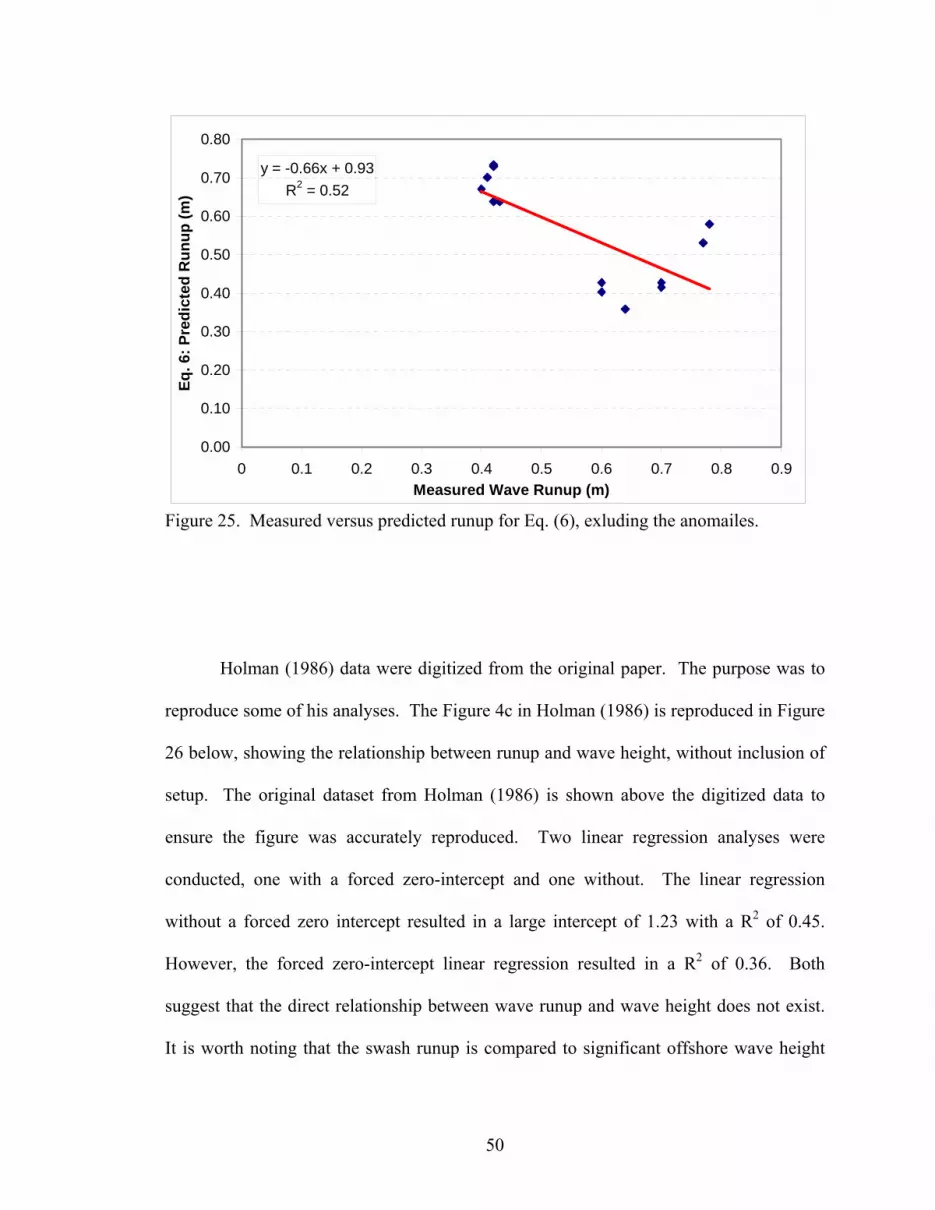
25). A similar trend as the predicted runup from Eq. (7) was observed, with a slightly

reduced R2 of 0.52. The two clusters in the data again illustrate an over and under

prediction of the erosive and accretionary waves.

49

y = 0.76xR2 = 0.76

0.00

0.10

0.20

0.30

0.40

0.50

0.60

0.70

0 0.1 0.2 0.3 0.4 0.5 0.6 0.7 0.8 0.9Measured Wave Runup (m)

Eq. 4

: Pre

dict

ed R

unup

(m)

Figure 23. Measured versus predicted runup for Eq. (4), excluding the anomalies.

y = -1.09x + 1.13R2 = 0.60

0.00

0.10

0.20

0.30

0.40

0.50

0.60

0.70

0.80

0.90

0 0.1 0.2 0.3 0.4 0.5 0.6 0.7 0.8 0.9Measured Wave Runup (m)

Eq. 7

: Pre

dict

ed R

unup

(m)

Figure 24. Measured versus predicted runup for Eq. (7), excluding the anomalies.

50

y = -0.66x + 0.93R2 = 0.52

0.00

0.10

0.20

0.30

0.40

0.50

0.60

0.70

0.80

0 0.1 0.2 0.3 0.4 0.5 0.6 0.7 0.8 0.9Measured Wave Runup (m)

Eq. 6

: Pre

dict

ed R

unup

(m)

Figure 25. Measured versus predicted runup for Eq. (6), exluding the anomailes.

Holman (1986) data were digitized from the original paper. The purpose was to

reproduce some of his analyses. The Figure 4c in Holman (1986) is reproduced in Figure

26 below, showing the relationship between runup and wave height, without inclusion of

setup. The original dataset from Holman (1986) is shown above the digitized data to

ensure the figure was accurately reproduced. Two linear regression analyses were

conducted, one with a forced zero-intercept and one without. The linear regression

without a forced zero intercept resulted in a large intercept of 1.23 with a R2 of 0.45.

However, the forced zero-intercept linear regression resulted in a R2 of 0.36. Both

suggest that the direct relationship between wave runup and wave height does not exist.

It is worth noting that the swash runup is compared to significant offshore wave height

51

measured at 8 m water depth, and not to breaker height. As shown in Figure 26, for the

same wave height, a large variation of wave runup values were measured, which does not

seem to be reasonable. It is not clear how and why a 1 m wave induced a 2.5 m swash

runup, while a 4 m wave induced less than 2 m of swash runup. It is questionable as to

how a 1 m offshore wave can induce a greater swash runup as compared to a 4 m

offshore wave.

The Figure 7c in Holman (1986) showing the relationship between surf similarity

and swash runup (minus setup) is reproduced in Figure 27. The measured swash runup

was normalized with offshore wave height. A linear regression analysis was conducted,

resulting in a R2 of 0.62. An exponential fit was also attempted (Figure 27). The

correlation coefficient was improved slightly, 0.69 versus 0.62, as compared to the linear

fit.

52

Holman '86: Figure 4

y = 0.44x + 1.23R2 = 0.45

y = 0.98xR2 = 0.36

0.00

0.50

1.00

1.50

2.00

2.50

3.00

3.50

4.00

0.00 0.50 1.00 1.50 2.00 2.50 3.00 3.50 4.00

Hs (m)

R2

(m)

Series1 Linear (Series1) Linear (Series1)

Figure 26. Figure 4c from Holman (1986) comparing swash runup (minus setup) and offshore significant wave height (above); the digitized data from Figure 4 (Holman, 1986) with two linear regression analyses (below).

53

Holman '86 Fig. 7

y = 0.46x - 0.04R2 = 0.62

y = 0.83x + 0.20

y = 0.25e0.58x

R2 = 0.69

0

0.5

1

1.5

2

2.5

3

3.5

0 0.5 1 1.5 2 2.5 3 3.5 4

Surf Similarity

R2

Series1 eq.6 Linear (Series1) Linear (eq.6) Expon. (Series1)

Figure 27. Figure 7c from Holman (1986) comparing swash runup (minus setup) and the surf similarity parameter (above); the digitized data from Figure 4 (Holman, 1986) with a linear and exponential regression analysis (below).

54

Recall, Douglass (1992) re-analyzed the Holman (1986) data set used in Eq. (6)

and found no correlation between runup and beach-face slope. Douglass further argued

that beach slope is a dependent variable free to respond to the incident wave energy and

should not be included in a runup prediction. In practice, beach face slope is a difficult

parameter to define and determine. Except for Stockdon et al. (2006), a clear definition

of beach slope is not given in most studies. However, the Stockdon et al. (2006)

definition of beach slope is very specific for video measurements and is difficult to utilize

for other methods. In the present study, the slope was defined over that portion of the

beach extending roughly 1 m landward and seaward from the still-water shoreline. Based

on this definition, the Holman (1986) dataset overall had a tan β = 0.08 to 0.17 across the

swash zone; the SUPERTANK dataset had a tan β = 0.09 to 0.15 across the swash zone.

The resulting beach-profiles from SUPERTANK under accretionary waves tended to

have slopes of 0.13 to 0.20, whereas the beach-profiles from erosional waves had slopes

of 0.08 to 0.14 (Table 1). Nielsen and Hanslow (1991) also discussed the difficultly in

defining beach slope, whether across the beach face or surf zone, with the presence of

bars on intermediate beaches further complicating the measurement of beach slope.

Including the beach slope thus adds ambiguity in applying the empirical formulas. In

addition, Douglass (1992) omitted the beach slope term from the Holman (1986) dataset,

arguing that the wave steepness term in the surf similarity parameter was responsible for

ξ’s predictive capability, rather than the inclusion of slope. This further suggests that the

use of the slope term in runup predictions not only induces more uncertainties, but is also

generally unnecessary.

55

However, the inclusion of slope may be required under certain circumstances.

For a very gentle beach, a large swash excursion is associated with a fixed runup, as

compared to a steep beach. It is reasonable to argue that if infiltration, saturation, and

bottom friction are significant, beach slope cannot be neglected. However, this is beyond

the scope of this study and is also not the case for most of the existing studies reviewed

(Guza and Thornton, 1982; Nielsen and Hanslow, 1991; Hanslow and Nielsen, 1993;

Ruggiero et al., 1996; Stockdon et al., 2006). Some experiment data have shown that the

friction loss due to wave propagation is small (Komar, 1998).

Determining offshore wave height may also cause uncertainty. In most field

studies, the offshore wave height was taken to be the value measured at a wave gage in

the study area. Similarly, here it is taken as that from the offshore-most gauge. Under

extreme storm conditions in which wave gauges often fail, estimating the offshore wave

height may not be straightforward (Wang et al., 2006). The definition of an offshore

wave height varies between studies, in which it is often taken at whatever depth the

instrument is deployed (Guza and Thornton, 1981; Guza and Thornton, 1982; Holman,

1986; Stockdon et al., 2006). Stockdon et al. (2006) concluded that runup was better

predicted using breaking wave height when it is available; however the often lack of

measured breaking wave height was argued as the reason for the use of offshore wave

height for predicting runup. Theoretically, the beach slope and wave characteristics are

contributing factors in the breaker height and type (Nielsen and Hanslow, 1991).

Therefore, using breaking wave height may indirectly incorporate these factors.

56

Eq. (10) was applied to examine the three-dimensional LSTF data. The wave

runup was not directly measured at LSTF. It is assumed here that the maximum runup is

equal to the upper limit of beach-profile change. This is a reasonable assumption, based

on the SUPERTANK data. For the spilling wave case, using the upper limit of beach

change at 0.23 m as the value for total wave runup, the breaking wave height of 0.26 m

resulted in an over-prediction of 13%. For the plunging wave case, the upper limit of

beach change was 0.26 m, which is almost equal to the 0.27 m breaking wave height.

Based on these limited results, the LSTF results support the predictive capabilities of the

new formula (Eq. 10). It is worth noting that the 1.5 x 10 -3 m (0.15 mm) sediment used

in the LSTF experiments is finer than the 2.2 x 10 -2 m (0.22 mm) used in the

SUPERTANK experiment.

A Conceptual Derivation of the Proposed Wave Runup Model

Assuming a normally incident wave and neglecting longshore variations and

infiltration, the major forces acting on a water element in the swash zone in the cross-

shore direction, x, (Fig. 28) can be balanced as:

2sin8

xx

Vfg x y z x yV x y zt

ρ β ρ ρ ∂− Δ Δ Δ − Δ Δ = Δ Δ Δ

∂ (11)

where, ρ = density of water; g = gravitational acceleration; Δx, Δy, and Δz, = length,

width, and height, of the water element, respectively; β = beach slope; f = a friction

coefficient; and Vx = velocity. Eq. (11) can be reduced to

2sin8

xx

V fg Vt z

β∂= − −

∂ Δ (12)

57

Figure 28. Schematic drawing of forces acting on a water element in the swash zone.

Assuming the friction force is negligible, an assumption supported by experiments

discussed in Komar (1998), Eq. (12) is further reduced to

sinxV gt

β∂= −

∂ (13)

Integrating Eq. (13) with respect to time, yields

sinx oV V gt β= − (14)

where, Vo = initial velocity. Integrating Eq. (14) again with respect to time gives the

swash excursion, x, as a function of time, t:

2

( ) sin2o

gtx t V t β= − (15)

From Eq. (14), the maximum uprush occurs at a time, tmax, when the velocity becomes

zero:

max sinoVt

g β= (16)

Vx

ρgΔxΔyΔz β

β

τb

58

with a corresponding value of maximum uprush of

2

max( )2 sin

oVx tg β

= (17)

Assuming a small and planar foreshore slope (Shen and Meyer, 1963; Mase, 1988;

Baldock and Holmes, 1999), i.e. tan β ≈ sin β, the elevation of the maximum swash

uprush Rsr_max,

2 2

_ max max( ) tan tan2 sin 2

o osr

V VR x tg g

β ββ

= = ≈ (18)

Eq. (18) suggests that the maximum elevation of swash runup is not a function of beach

slope when friction forcing is neglected.

The initial velocity Vo can be approximated by the velocity of the wave, Cg. In

shallow water, the wave velocity is limited by the local water depth, hl.

o g lV C gh≈ = (19)

Assuming a linear relationship between local breaking wave height, Hbl, and the water

depth, hl

bl lH hγ= (20)

where γ is the breaker index. Eq. (19) then becomes

2 2 blo g

HV C gγ

≈ = (21)

Substituting Eq. (21) into Eq. (18)

2

_ max 2 2 2o bl bl

srV gH HR

g gγ γ= = = (22)

59

It is reasonable to assume that the initial Vo can be taken at the main breaker line, using

significant breaker height, Hbs. Eq. (22) becomes

_ max 2bs

sr bsHR Hαγ

= = (23)

where α = 1/2γ. Eq. (23) indicates a linear relationship between breaking wave height

and the maximum swash runup, supporting the findings from the SUPERTANK

experiment.

Kaminsky and Kraus (1994) examined a large dataset, including both laboratory

and field measurements, on breaking wave criteria. They found that the majority of the γ

values range from 0.6 to 0.8, which yields α values from 0.63 to 0.83. Based on the

discussion of Figs. 15 through 18, the swash runup constitutes approximately 83% of the

total wave runup. Adding the 17% contribution from the wave setup, then the total wave

runup, Rmax, is roughly proportional to the breaking wave height at unity, further

supporting the new model developed from the SUPERTANK dataset.

60

Conclusions

The SUPERTANK data indicate that the vertical extent of wave runup above

mean water level on a non-scarped beach is approximately equal to the significant

breaking wave height. A simple formula for predicting the maximum wave runup, Rmax:

max bsR H= , was developed and proven by a conceptual derivation. The new model was

applied to the 3-dimensional LSTF experiments, and accurately reproduced the measured

wave runup. By including the surf similarity parameter, as with several existing

empirical formulas, the accuracy of the calculated wave runup decreased as compared to

the measured values. In addition, the upper limit of beach change was found to be

approximately equivalent to the maximum vertical excursion. Because the maximum

runup was found to be directly related to breaker height, and the upper limit of beach

change was approximately equal to the maximum runup, the breaker height can be used

to assess morphological changes on beaches due to runup. In other words, UL =Rmax =Hb.

For monochromatic waves, the measured wave runup was much smaller than the

breaking wave height. The lack of low-frequency modulation limits the wave runup for

monochromatic waves. The hydrodynamics and beach-profiles resulting from regular

waves are not comparable to the real-world. Therefore, results from studies with

monochromatic waves are not useful in predicting wave runup and beach changes for

natural beaches.

61

An exception to the direct relationship between breaking wave height, runup and

upper limit of beach change concerns dune or beach scarping. The steep scarp

substantially limits the uprush of swash motion, resulting in a much reduced maximum

level as compared with the non-scarping cases. The nearly vertical scarp also induces

technical difficulties of measuring the runup using wire gages. Most predictive equations

are not expected to apply to scarped cases. Because the actual upper limit of beach

change is controlled by the elevation of the backbeach or dune, the upper limit of wave

runup was not found to correlate with the breaker height for these cases.

Based on the SUPERTANK and LSTF experiments, the upper limit of beach-

profile change was found to be approximately equal to the maximum vertical excursion

of wave runup for waves between 0.20 and 1.00 m. Therefore, the limit of wave runup

can serve as an estimate of the landward limit of beach change. Physical situations that

are exceptions to this direct relationship are those with beach or dune scarping.

Accurately predicting the maximum elevation of wave runup was best predicted using the

breaker height. The applicability of this relationship will contribute to predictive

capabilities of assessing beach change for nourishment and structure designs, engineering,

and many other coastal management practices.

62

References

Baldock, T.E. and Holmes, P., 1999. Simulation and prediction of swash oscillations on a

steep beach. Coastal Engineering, 36, 219-242.

Battjes, J.A., 1971. Runup distributions of waves breaking on slopes. Journal of

Waterways, Harbors and Coasts Engrg. Div., ASCE, 97 WW1, 91-114.

Battjes, J.A., 1974. Computations of set-up, longshore currents, run-up overtopping due

to wind-generated waves. Rep. 74-2, Delft Univ. Technol., Delft, The

Netherlands.

Bowen, A.J., Inman, D.L., and Simmons, V.P., 1968. Wave “set-down” and “set-up.” J.

Geophys. Res., 73(8), 2569-2577.

Bruun, P., 1954. Coastal erosion and the development of beach profiles. Tech. Memo. No.

44, Beach Erosion Board, U.S. Army Corps of Engineers.

Dean, R.G., 1977. Equilibrium beach profiles: U.S. Atlantic and Gulf coasts. Ocean

Engineering Rep. No. 12, Dept. of Civil Eng., Univ. of Delaware, Newark, DE.

Douglass, S.L., 1992. Estimating extreme values of run-up on beaches. J. Waterway,

Port, Coastal and Ocean Eng., 118, 220-224.

Galvin, C.J., Waves breaking in shallow water, in Waves on Beaches and Resulting

Sediment Transport, 462 pp., Academic, New York, 1972.

63

Guza, R.T., and Thornton, E.B., 1981. Wave set-up on a natural beach. J. Geophys. Res.,

86(C5), 4133-4137.

Guza, R.T., and Thornton, E.B., 1982. Swash oscillations on a natural beach. J. Geophys.

Res. 87(C1), 483-490.

Hamilton, D.G., Ebersole, B.A., Smith, E.R., and Wang, P., 2001. Development of a

large-scale laboratory facility for sediment transport research. Technical Report

ERDC/SCH-TR-01-22, U.S. Army Engineer Research and Development Center,

Vicksburg, Mississippi.

Hanslow, D., and Nielsen, P., 1993. Shoreline set-up on natural beaches. Journal of

Coastal Research SI (15), 1-10.

Holland, K.T., Raubenheimer, B., Guza, R.T., and Holman, R.A., 1995. Runup

kinematics on a natural beach. J. Geophys. Res., 100(C3), 4985-4993.

Holman, R.A., 1986. Extreme value statistics for wave run-up on a natural beach. Coastal

Eng., 9, 527-544.

Holman, R.A., and Guza, R.T., 1984. Measuring runup on a natural beach. Coastal Eng.,

8: 129-140.

Holman, R.A., and Sallenger, A.H., 1985. Setup and swash on a natural beach. J.

Geophys. Res., 90(C1), 945-953.

Howd, P.A., Oltman-Shay, J., Holman, R.A., 1991. Wave variance partitioning in the

trough of a barred beach. Journal of Geophysical Research 96 (C7), 12781-

12795.

64

Huntley, D.A., Davidson, M., Russell, P., Foote, Y., and Hardisty, J., 1993. Long waves

and sediment movement on beaches: Recent observations and implications for

modeling. J. Coastal Res., 15, 215-229.

Iribarren, C.R. and Nogales, C., 1949. Protection des portes. XVII International

Navigation Congress, Lisbon, SII-1.

Kaminsky, G. and Kraus, N.C., 1994. Evaluation of depth-limited breaking wave criteria.

Proceedings of Ocean Wave Measurement and Analysis, New York: ASCE Press,

pp. 180-193.

Komar, P. D., Beach Processes and Sedimentation, 2nd Ed., 544 pp., Prentice Hall, New

Jersey, 1998.

Kraus, N.C., Larson, M., and Wise, R.A., 1999. Depth of closure in beach fill design:

Proc. 1999 National Conference on Beach Preservation Technology, FSBPA,

Tallahassee, FL.

Kraus, N.C., and Smith, J.M., (Eds.) 1994. SUPERTANK Laboratory Data Collection

project, Volume 1: Main text. Tech. Rep. CERC-94-3, U.S. Army Eng.

Waterways Experiment Station, Coastal Eng.. Res. Center, Vicksburg, MS.

Kraus, N.C., Smith, J.M., and Sollitt, C.K. 1992. SUPERTANK Laboratory data

collection project. Proc.23rd Coastal Eng. Conf, ASCE, 2191-2204.

Mase, H., 1988. Spectral characteristics of random wave run-up. Coastal Engineering 12,

175-189.

Nielsen, P. 1988. Wave setup: A field study. J. Geophys. Res., 93(C12), 15,643-652.

Nielsen, P. and Hanslow, D.J., 1991. Wave runup distributions on natural beaches.

Journal of Coastal Research 7 (4), 1139-1152.

65

Raubenheimer, B., Guza, R.T. and Elgar, S., (1996). Wave transformation across the

inner surf zone. J. Geophys. Res., 101(C10):25589-25597.

Ruessink, B.G., Kleinhans, M.G., and van den Beukel, P.G.L., 1998. Observations of

swash under highly dissipative conditions, J. Geophys. Res., 103, 3111–3118.

Ruggiero, P., Komar, P.D., McDougal, W.G., and Beach, R.A., 1996. Extreme water

levels, wave runup, and coastal erosion. Proceedings of the 25th Coastal

Engineering Conference, Amer. Soc. Civil Eng., pp. 2793-2805.

Ruggiero, P., Holman, R.A., and Beach, R.A., 2004. Wave run-up on a high-energy

dissipative beach. J. Geophys. Res., 109(C06025), 1-12.

Sallenger, A.H., 2000. Storm impact scale for barrier island. J. of Coastal Research 16,

890-895.

Shen, M.C. and Meyer, R.E., 1963. Climb of a bore on a beach 3: run-up. J. Fluid Mech..

16, 113-125.

Short, A.D., 1979a. Wave power and beach stages: A global model. Proc. 17th Int. Conf.

Coastal Eng., Hamburg, 1978, pp. 1145-1162.

Short, A.D., 1979b. Three dimensional beach stage model. Journal of Geology, 87: 553-

571.

Stockdon, H.F., Holman, R.A., Howd, P.A., and Sallenger, A.H., 2006. Empirical

parameterization of setup, swash, and runup. Coastal Eng., 53, 573-588.

Wang, P., Ebersole, B.A., Smith, E.R., and Johnson, B.D., 2002. Temporal and special

variations of surf-zone currents and suspended-sediment concentration. Coastal

Eng., 46, 175-211.

66

Wang, P., and Davis, R.A., Jr., 1998. A beach profile model for a barred coast – case

study from Sand Key, west-central Florida. J. Coastal Res., 14, 981-991.

Wang, P., and Davis, R.A. Jr., 1999. Depth of closure and equilibrium beach profile: A

case study from sand key, west-central Florida, Shore and Beach 67 (2 &3), 33-42.

Wang, P., and Kraus, N.C., 2005. Beach profile equilibrium and patterns of wave decay

and energy dissipation across the surf zone elucidated in a large-scale laboratory

experiment. J. Coastal Res., 21, 522-534.

Wang, P., Kirby, J.H., Haber, J.D., Horwitz, M.H., Knorr, P.O., and Krock, J.R., 2006.

Morphological and sedimentological impacts of Hurricane Ivan and immediate post-

storm beach recovery along the northwestern Florida barrier-island coasts, J. Coastal

Res., 22(6), 1,382-1,402.

Wright, L.D., Chappell, J., Thom, B.G., Bradshaw, M.P. and Cowell, P., 1979a.

Morphodynamics of reflective and dissipative beach and inshore systems:

Southeastern Australia. Marine Geology, 32: 105-140.

Wright, L.D., Thom, B.G., and Chappell, J., 1979b. Morphodynamic variability of high

energy beachs. Proc. 16th Int. Conf. Coastal Eng., Hamburg, 1978, 1180-1194.

Wright, L.D., and Short, A. D., 1984, Morphodynamic variability of surf zones and

beaches: A Synthesis: Marine Geology, v. 56, 93-118.

Yamamoto, Y., Tanimoto, K., and Harshinie, K.G. 1994. Run-up of irregular waves on

gently sloping beach. Proc.23rd Coastal Eng. Conf, ASCE, 689-703.

67

Appendices

68

Appendix I - Notation

The following symbols were used in this paper: A shape parameter relating to grain size and fall velocity Cg wave group velocity f friction coefficient g gravitational acceleration h still-water depth H wave height Hb breaking wave height Hbl local breaking wave height Hbs significant breaking wave height Hb_h high frequency component of wave height at the breaker line Hb_l low frequency component of wave height at the breaker line hl local water depth Ho significant deepwater wave height Hsl_h high frequency component of wave height at the shoreline line Hsl_l low frequency component of wave height at the shoreline line LL lower limit of beach change Lo deepwater wavelength n spectral peakness N Dean number Rmax maximum swash runup Rs significant wave runup Rsr_max elevation of maximum swash uprush R2 2% exceedence of runup T wave period tmax time of maximum swash excursion Tp peak wave period UL upper limit of beach change Vo initial velocity Vx velocity of a water particle in the cross-shore direction x cross-shore coordinate β beach slope βf foreshore beach slope γ breaker index Δx length of a water particle Δy width of a water particle

69

Δz height of a water particle η wave setup

Mη wave setup under monochromatic waves

slη wave setup at the shoreline ξ surf-similarity parameter ρ water density ω sediment fall velocity