Embed Size (px)
Citation preview
DOCTORA L T H E S I S
Magnetic Resonance Sounding (MRS) in Groundwater Exploration,
with Applications in Laos and Sweden
Nils Perttu
Nils Perttu M
agnetic Resonance Sounding (M
RS) in G
roundwater E
xploration, with A
pplications in Laos and Sweden
Department of Civil, Environmental and Natural resources engineeringDivision of Geosciences and Environmental Engineering
ISSN: 1402-1544 ISBN 978-91-7439-306-4
Luleå University of Technology 2011

Magnetic Resonance Sounding (MRS) in groundwater exploration,with applications in Laos and Sweden
Nils Perttu
Doctoral thesis in the subjectApplied Geophysics
Division of Geosciences and Environmental EngineeringDepartment of Civil, Environmental and Natural resources engineering
Luleå University of Technology
Printed by Universitetstryckeriet, Luleå 2011
ISSN: 1402-1544 ISBN 978-91-7439-306-4
Luleå 2011
www.ltu.se

“It is wise to bring some water, when one goes out to look for water”
Arab Proverb

ACKNOWLEDGEMENT
The research presented in this thesis was carried out at the division of Geosciences at Luleå University
Development Cooperation Agency (SIDA-Sarek), research in memory of J. Gust. Richert (SWECO) and Seth Kempe’s Memorial fund.
I would like to express my deepest gratitude to my supervisor Professor Sten-Åke Elming for giving me the opportunity to enter the world of research and working with groundwater problems in
of articles and the thesis and for believing in me throughout the work. Likewise I am also grateful to my assistant supervisor, Professor Dattatray Parasnis for his guidance concerning my work and courses. My warmest and sincerest gratitude goes to Anatoly Legchenko for inviting me to Grenoble; Teaching me MRS both in theory and in practice and sharing his expertise and long experience in working with MRS.
Khamphouth Phommasone, Kamhaeng Wattanasen Lena Persson, Mikael Erlström and Jean-Michel Vouillamoz have all made important contributions to my articles. A special thank goes to Hans Thunehed, Håkan Mattsson, Lennart Wikberg and Bo Löfroth for sharing their long experience in working with geophysics and giving a helping hand when needed. Also, without handy persons like Roger Lindfors and Milan Vnuk, this university would go under and they deserve a special recognition. My sincere gratitude goes to the anonymous reviewers within the small MRS research community for taking their time to constructively criticize and improve my articles.
I want to thank past and present members of the applied geophysics group and all my colleagues at the Division of Geosciences and Environmental Engineering for their friendship and support. Finally, I send my loving thanks to my family, relatives and friends and especially my girlfriend Anna-Maria and my daughter Alma for encouraging and supporting me through out my work.
Thank you!
Nils PerttuAugust, 2011Luleå, Sweden

ABSTRACT
Water is essential for all life on the planet, sustaining and ensuring the earth’s ecosystem. Groundwater from a global perspective provides about 50 % of the potable- , 40 % of the industrial- and 20 % of the irrigation water. For drinking water, deep groundwater has many advantages compared to surface water and shallow groundwater, since it demands little or no treatment and the access is secured against
if it is made without knowing the groundwater potential, therefore development of techniques for exploration are of high priority.
salinity, e.g. electrical conductivity and electric permittivity, which can be determined from Vertical Electrical Sounding (VES) and Ground Penetrating Radar (GPR) measurements, respectively. Magnetic Resonance Sounding (MRS), based on the principle of nuclear magnetic resonance, is a relatively new, non invasive technique, which in contrast to other geophysical techniques gives a direct measure of the free water content, but also the pore size distribution with depth. With MRS it is possible to determine both storage and hydraulic related parameters far less ambiguously than with classical geophysical techniques. This thesis presents four studies, where the MRS technique have been tested and developed in combination with other geophysical techniques in three different geological environments; (1) The sedimentary basin of Vientiane, Laos, with naturally occurring salt in the bedrock as shallow as 50 m in depth, which inevitably affects drinking and irrigation water from deep wells; (2) In karst limestone, on the island of Gotland, Sweden, where saltwater intrusion, both recent and relic together with pollution from pesticides and fertilizers are major threats to an already exhausted drinking water resource; (3) Test of the MRS spin-echo (SE) technique in Norrbotten, Sweden, where the presence of magnetic rocks and sediments have made it impossible to do MRS with a standard measuring procedure.
and distinguish freshwater aquifers from clays. The electrical conductivity (EC) of the aquifers determined from VES correlates well with EC of water collected from shallow and deep wells, which makes the method promising for future water quality estimation in the Vientiane basin. In Gotland (2), the performance of MRS, VES, GPR and Radiomagnetotelluric (RMT) were tested. The use of multiple techniques has shown to give a more coherent interpretation, but MRS and RMT showed
of large scale magnetic gradients on the MRS signals but also the reliability of MRS SE result. The MRS SE technique has further been tested for different soil types. The measuring procedure has subsequently been tested and optimized to meet conditions of magnetic environments.
Keywords: geophysics; magnetic resonance sounding (MRS); spin echo; aquifer; groundwater; resistivity; salinity; Gotland; Khorat Plateau; Laos; Norrbotten.

CONTENTS
1 INTRODUCTION ...................................................................................................... 11.1 Aims.................................................................................................................... 3
2 METHODS ................................................................................................................. 42.1 Magnetic Resonance Sounding (MRS)............................................................... 4
2.1.1 The principle of NMR..................................................................................... 42.1.2 The MRS method............................................................................................ 62.1.3 Relaxation of the signal .................................................................................. 82.1.4 MRS related to hydrogeological parameters................................................. 102.1.5 ....................................................................... 122.1.6 .............................................................................. 14
2.2 DC Resistivity................................................................................................... 162.2.1 Estimation of the electrical conductivity (EC) of water ............................... 172.2.2 Water quality parameters related to EC of water .......................................... 18
2.3 Radiomagnetotelluric (RMT)............................................................................ 182.4 Ground Penetrating Radar (GPR) ..................................................................... 192.5 Complex resistivity (CR; In laboratory) ........................................................... 19
3 MAIN RESULTS AND CONCLUSIONS ............................................................... 203.1 Vientiane Basin, Laos ....................................................................................... 20
3.1.1 Main results................................................................................................... 203.1.2 Conclusions................................................................................................... 25
3.2 Gotland, Sweden ............................................................................................... 253.2.1 Main results................................................................................................... 253.2.2 Conclusions................................................................................................... 28
3.3 Luleå, Sweden................................................................................................... 293.3.1 Main results................................................................................................... 293.3.2 Conclusions................................................................................................... 33
4 SUMMARY .............................................................................................................. 335 REFERENCES ......................................................................................................... 35APPENDED PAPERS (I-IV)

LIST OF PAPERS
This thesis consists of the following four papers, henceforth referred to by their roman numerals.
I Characterization of aquifers in the Vientiane Basin, Laos, using Magnetic Resonance Sounding and Vertical Electrical Sounding.Perttu, N., Wattanasen, K., Phommasone, S-Å., Elming (2011)Journal of Applied Geophysics, 73: 207-220.
II Determining Water Quality Parameters of Aquifers in the Vientiane Basin, Laos, Using Geophysical and Water Chemistry Data.Perttu, N., Wattanasen, K., Phommasone, S-Å., Elming (2011)Near Surface Geophysics, 9: 381-395.
III Magnetic Resonance Sounding and Radiomagnetotelluric measurements used to characterize a limestone aquifer in Gotland, Sweden.Perttu, N., Persson, L., Erlström, M. and Elming, S-Å. (2011)Submitted to Journal of Hydrology
IV Field evaluation of the MRS Spin-Echo method under geological conditions typical for the northern part of SwedenPerttu, N., Legchenko, A., Vouillamoz, J.M. and Elming, S-Å (2011)Submitted to Journal of Applied Geophysics
Paper I and II were reprinted with kind permission by Elsevier Science and ScholarOne Inc, respectively.

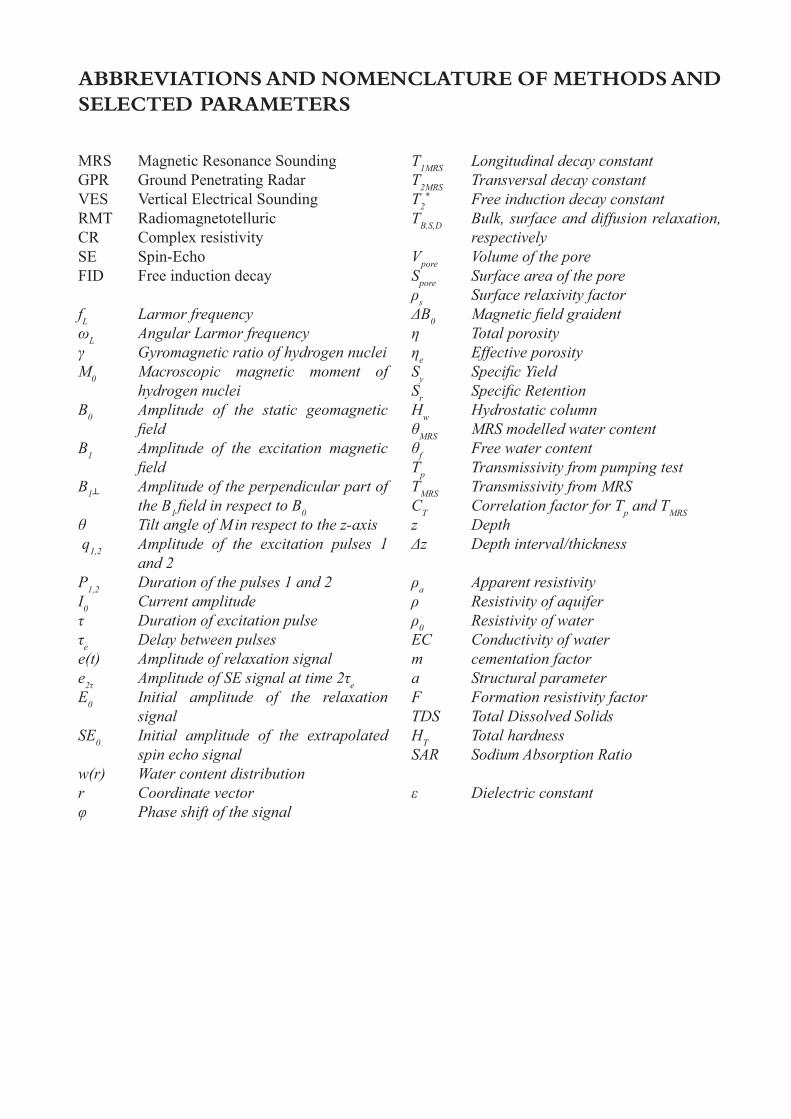
ABBREVIATIONS AND NOMENCLATURE OF METHODS AND SELECTED PARAMETERS
MRS Magnetic Resonance SoundingGPR Ground Penetrating RadarVES Vertical Electrical SoundingRMT RadiomagnetotelluricCR Complex resistivitySE Spin-EchoFID Free induction decay
fL Larmor frequencyL Angular Larmor frequency
M0 Macroscopic magnetic moment of hydrogen nuclei
B0 Amplitude of the static geomagnetic
B1 Amplitude of the excitation magnetic
B Amplitude of the perpendicular part of the B1 0
in respect to the z-axis q1,2 Amplitude of the excitation pulses 1
and 2P1,2 Duration of the pulses 1 and 2I0 Current amplitude
e Delay between pulsese(t) Amplitude of relaxation signale eE0 Initial amplitude of the relaxation
signalSE0 Initial amplitude of the extrapolated
spin echo signal w(r) Water content distributionr Coordinate vector
1MRS Longitudinal decay constant2MRS
2* Free induction decay constant
B,S,D Bulk, surface and diffusion relaxation, respectively
Vpore Volume of the poreSpore Surface area of the pore
s Surface relaxivity factor0
e Effective porositySySrHw Hydrostatic column
MRS MRS modelled water contentf Free water contentp
MRSC p MRSz Depth
a Apparent resistivity
0 Resistivity of waterEC Conductivity of waterm cementation factora Structural parameterF Formation resistivity factor
HSAR Sodium Absorption Ratio

1
INTRODUCTION
1 INTRODUCTION
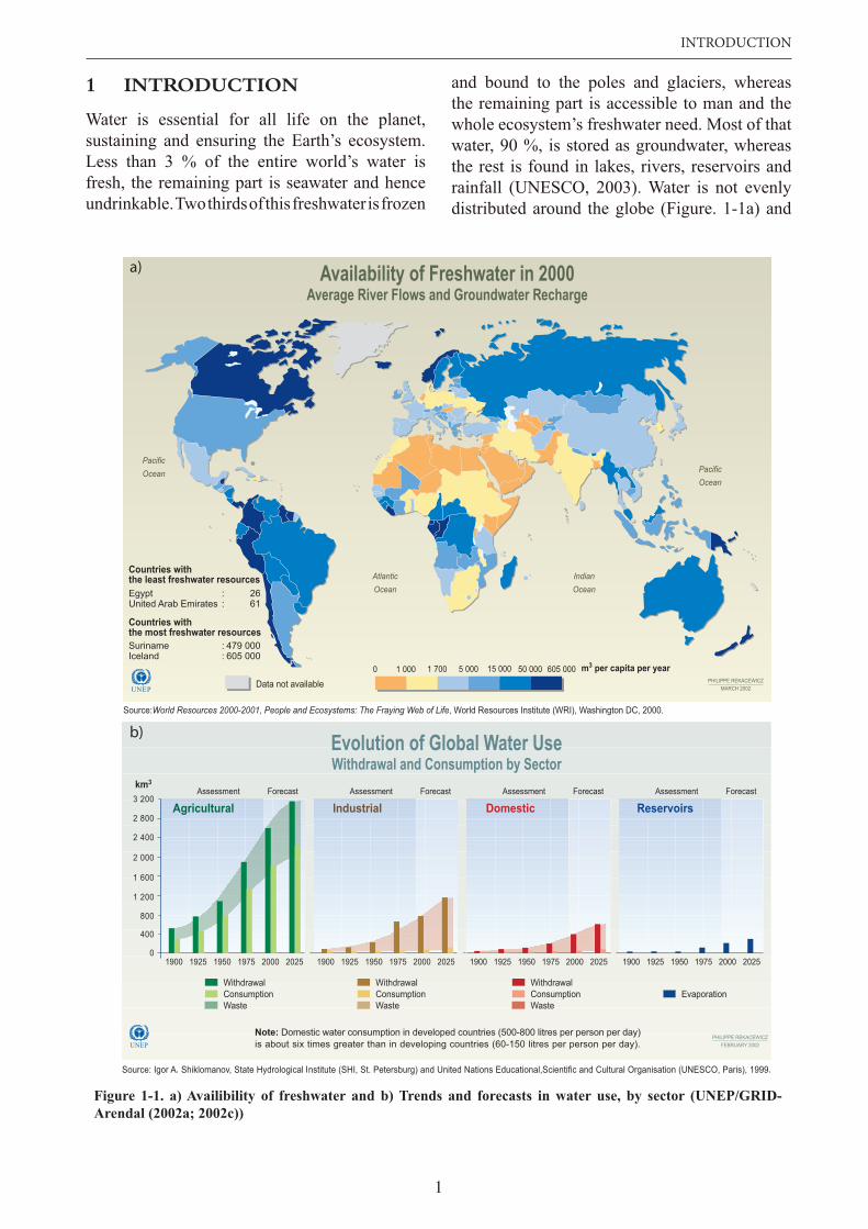
Water is essential for all life on the planet, sustaining and ensuring the Earth’s ecosystem. Less than 3 % of the entire world’s water is fresh, the remaining part is seawater and hence undrinkable. Two thirds of this freshwater is frozen
and bound to the poles and glaciers, whereas the remaining part is accessible to man and the whole ecosystem’s freshwater need. Most of that water, 90 %, is stored as groundwater, whereas the rest is found in lakes, rivers, reservoirs and rainfall (UNESCO, 2003). Water is not evenly distributed around the globe (Figure. 1-1a) and
PacificOcean Pacific
Ocean
AtlanticOcean
IndianOcean
Source:World Resources 2000-2001, People and Ecosystems: The Fraying Web of Life, World Resources Institute (WRI), Washington DC, 2000.
Availability of Freshwater in 2000Average River Flows and Groundwater Recharge
479 000605 000
SurinameIceland
::
EgyptUnited Arab Emirates
2661
::
Countries withthe least freshwater resources
Countries withthe most freshwater resources
1 000 1 700 5 000 15 000 50 000 605 000 m3 per capita per year0
Data not availableUNEP MARCH 2002PHILIPPE REKACEWICZ
a)
b)
Figure 1-1. a) Availibility of freshwater and b) Trends and forecasts in water use, by sector (UNEP/GRID-Arendal (2002a; 2002c))
2
Magnetic Resonance Sounding (MRS) in groundwater exploration.
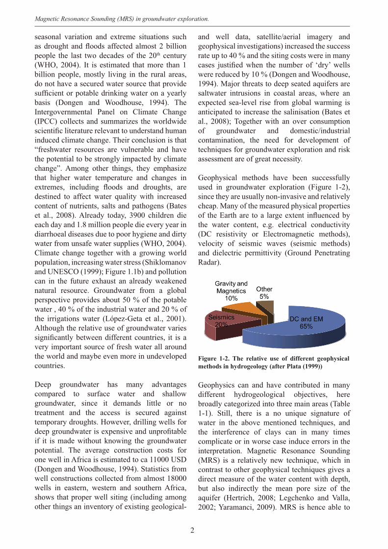
Figure 1-2. The relative use of different geophysical methods in hydrogeology (after Plata (1999))
seasonal variation and extreme situations such
people the last two decades of the 20th century (WHO, 2004). It is estimated that more than 1 billion people, mostly living in the rural areas, do not have a secured water source that provide
basis (Dongen and Woodhouse, 1994). The Intergovernmental Panel on Climate Change (IPCC) collects and summarizes the worldwide
induced climate change. Their conclusion is that “freshwater resources are vulnerable and have the potential to be strongly impacted by climate change”. Among other things, they emphasize that higher water temperature and changes in
destined to affect water quality with increased content of nutrients, salts and pathogens (Bates et al., 2008). Already today, 3900 children die each day and 1.8 million people die every year in diarrhoeal diseases due to poor hygiene and dirty water from unsafe water supplies (WHO, 2004). Climate change together with a growing world population, increasing water stress (Shiklomanov and UNESCO (1999); Figure 1.1b) and pollution can in the future exhaust an already weakened natural resource. Groundwater from a global perspective provides about 50 % of the potable water , 40 % of the industrial water and 20 % of the irrigations water (López-Geta et al., 2001). Although the relative use of groundwater varies
very important source of fresh water all around the world and maybe even more in undeveloped countries.
Deep groundwater has many advantages compared to surface water and shallow groundwater, since it demands little or no treatment and the access is secured against temporary droughts. However, drilling wells for
if it is made without knowing the groundwater potential. The average construction costs for one well in Africa is estimated to ca 11000 USD (Dongen and Woodhouse, 1994). Statistics from well constructions collected from almost 18000 wells in eastern, western and southern Africa, shows that proper well siting (including among other things an inventory of existing geological-
and well data, satellite/aerial imagery and geophysical investigations) increased the success rate up to 40 % and the siting costs were in many
were reduced by 10 % (Dongen and Woodhouse, 1994). Major threats to deep seated aquifers are saltwater intrusions in coastal areas, where an expected sea-level rise from global warming is anticipated to increase the salinisation (Bates et al., 2008); Together with an over consumption of groundwater and domestic/industrial contamination, the need for development of techniques for groundwater exploration and risk assessment are of great necessity.
Geophysical methods have been successfully used in groundwater exploration (Figure 1-2), since they are usually non-invasive and relatively cheap. Many of the measured physical properties
the water content, e.g. electrical conductivity (DC resistivity or Electromagnetic methods), velocity of seismic waves (seismic methods) and dielectric permittivity (Ground Penetrating Radar).
Geophysics can and have contributed in many different hydrogeological objectives, here broadly categorized into three main areas (Table 1-1). Still, there is a no unique signature of water in the above mentioned techniques, and the interference of clays can in many times complicate or in worse case induce errors in the interpretation. Magnetic Resonance Sounding (MRS) is a relatively new technique, which in contrast to other geophysical techniques gives a direct measure of the water content with depth, but also indirectly the mean pore size of the aquifer (Hertrich, 2008; Legchenko and Valla, 2002; Yaramanci, 2009). MRS is hence able to
3
INTRODUCTION
determine both storage and hydraulic related parameters far less ambiguous than classical geophysical techniques (Lubczynski and Roy, 2005).
MRS is today an established technique that has already shown very promising result in mapping and hydrogeological parameterization (Legchenko et al., 2004; Plata and Rubio, 2008; Vouillamoz et al., 2007b; Yaramanci et al., 2002) in different geological environments.
1.1 Aims
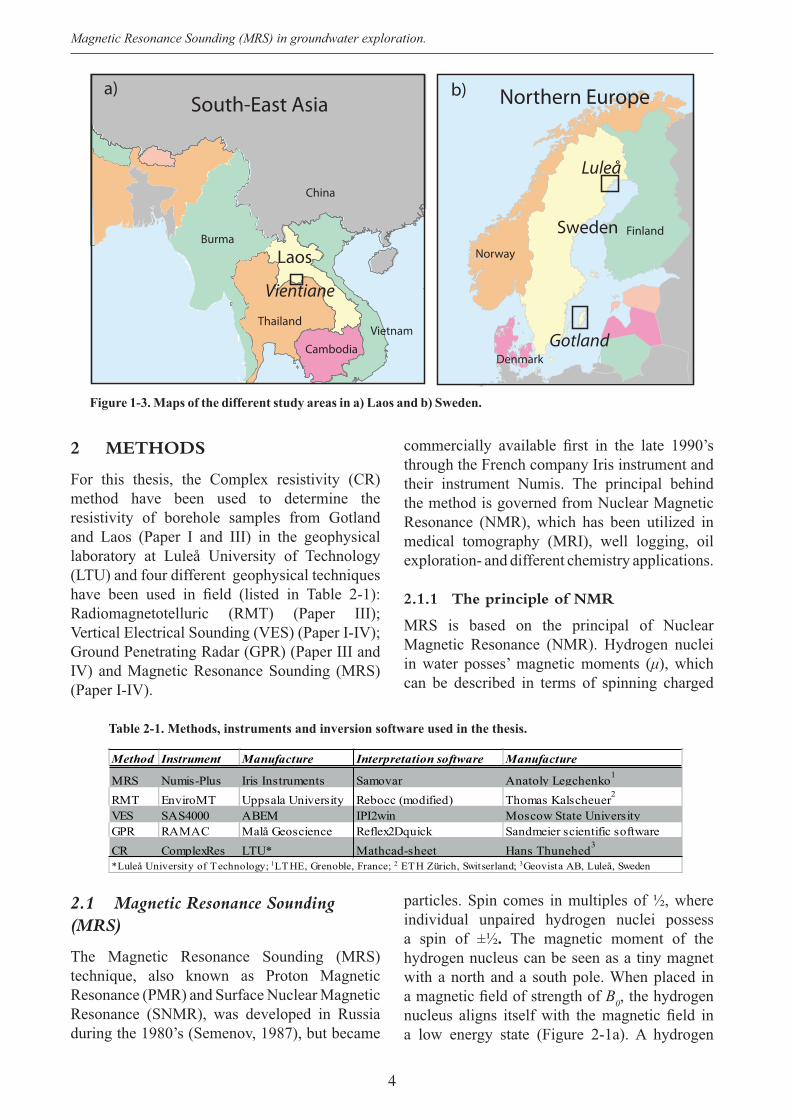
This thesis presents studies where the MRS technique has been tested in combination with other geophysical techniques in three different geological environments; (1) The sedimentary basin of Vientiane, Laos (Figure 1-3a), with naturally occurring salt in the bedrock as shallow as 50 m in depth, which inevitably affects drinking and irrigation water from deep wells; (2) In karst limestone, on the island of Gotland, Sweden, where saltwater intrusion, both recent and relic together with pollution from pesticides and fertilizers are major threats to an already exhausted drinking water supply (Figure 1-3b); (3) In Norrbotten, Sweden, where the presence of magnetic rocks and sediments have made it impossible to do MRS with a standard measuring procedure (Figure 1-3b). The MRS spin-echo
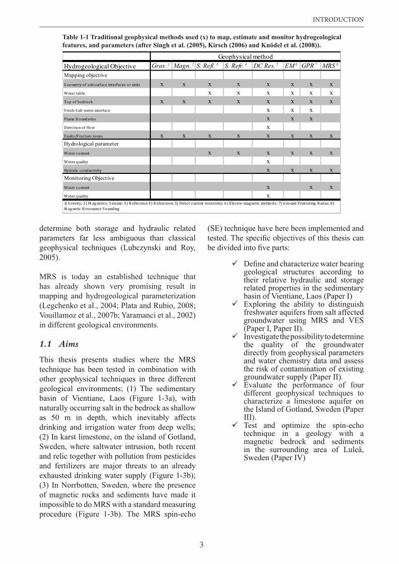
Table 1-1 Traditional geophysical methods used (x) to map, estimate and monitor hydrogeological features, and parameters (after Singh et al. (2005), Kirsch (2006) and Knödel et al. (2008)).
(SE) technique have here been implemented and
geological structures according to their relative hydraulic and storage related properties in the sedimentary basin of Vientiane, Laos (Paper I) Exploring the ability to distinguish freshwater aquifers from salt affected groundwater using MRS and VES (Paper I, Paper II).Investigate the possibility to determine the quality of the groundwater directly from geophysical parameters and water chemistry data and assess the risk of contamination of existing groundwater supply (Paper II).Evaluate the performance of four different geophysical techniques to characterize a limestone aquifer on the Island of Gotland, Sweden (Paper III).Test and optimize the spin-echo technique in a geology with a magnetic bedrock and sediments in the surrounding area of Luleå, Sweden (Paper IV)
Hydrogeological Objective Grav. 1 Magn. 2 S. Refl. 3 S. Refr. 4 DC Res. 5 EM 6 GPR 7 MRS 8
Mapping objectiveG eometry of subsurface interfaces or units x x x x x x x xWater table x x x x x xTop of bedrock x x x x x x x xFresh-S alt water interface x x xPlume B oundaries x x xDirection of flow xFaults/Fracture zones x x x x x x x xHydrological parameterWater content x x x x x xWater quality xHydralic conductivity x x x xMonitoring ObjectiveWater content x x xWater quality x
Geophysical method
1) G ravity; 2) M ag netics; S eismic 3) R eflection 4) R efraction; 5) Direct current resistivity; 6) Electro-mag netic methods; 7) G round Pentrating R adar; 8)
M ag netic R esonance S ounding
4
Magnetic Resonance Sounding (MRS) in groundwater exploration.
2 METHODS
For this thesis, the Complex resistivity (CR) method have been used to determine the resistivity of borehole samples from Gotland and Laos (Paper I and III) in the geophysical laboratory at Luleå University of Technology (LTU) and four different geophysical techniques
Radiomagnetotelluric (RMT) (Paper III); Vertical Electrical Sounding (VES) (Paper I-IV); Ground Penetrating Radar (GPR) (Paper III and IV) and Magnetic Resonance Sounding (MRS) (Paper I-IV).
through the French company Iris instrument and their instrument Numis. The principal behind the method is governed from Nuclear Magnetic Resonance (NMR), which has been utilized in medical tomography (MRI), well logging, oil exploration- and different chemistry applications.
2.1.1 The principle of NMR
MRS is based on the principal of Nuclear Magnetic Resonance (NMR). Hydrogen nuclei in water posses’ magnetic moments ( ), which can be described in terms of spinning charged
Figure 1-3. Maps of the different study areas in a) Laos and b) Sweden.
Sweden
Luleå
Gotland
Norway
Finland
Denmark
b)
Vientiane
Laos
VietnamCambodia
Thailand
Burma
China
a)South-East Asia Northern Europe
Method Instrument Manufacture Interpretation software Manufacture
MRS Numis-Plus Iris Instruments Samovar Anatoly Legchenko1
RMT EnviroMT Uppsala University Rebocc (modified) Thomas Kalscheuer2
VES SAS4000 ABEM IPI2win Moscow State University GPR RAMAC Malå Geoscience Reflex2Dquick Sandmeier scientific software CR ComplexRes LTU* Mathcad-sheet Hans Thunehed3
*Luleå University of Technology; 1LTHE, Grenoble, France; 2 ETH Zürich, Switserland; 3Geovista AB, Luleå, Sweden
Table 2-1. Methods, instruments and inversion software used in the thesis.
2.1 Magnetic Resonance Sounding (MRS)
The Magnetic Resonance Sounding (MRS) technique, also known as Proton Magnetic Resonance (PMR) and Surface Nuclear Magnetic Resonance (SNMR), was developed in Russia during the 1980’s (Semenov, 1987), but became
particles. Spin comes in multiples of ½, where individual unpaired hydrogen nuclei possess a spin of ±½. The magnetic moment of the hydrogen nucleus can be seen as a tiny magnet with a north and a south pole. When placed in
B0, the hydrogen
a low energy state (Figure 2-1a). A hydrogen
5
METHODS
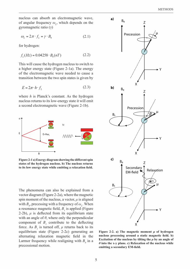
nucleus can absorb an electromagnetic wave, of angular frequency L, which depends on the
(2.1)
for hydrogen:
(2.2)
This will cause the hydrogen nucleus to switch to a higher energy state (Figure 2-1a). The energy of the electromagnetic wave needed to cause a transition between the two spin states is given by
(2.3)
where h is Planck’s constant. As the hydrogen nucleus returns to its low-energy state it will emit a second electromagnetic wave (Figure 2-1b).
Figure 2-1 a) Energy diagram showing the different spin states of the hydrogen nucleus. b) The nucleus returns
b)
E
B
E=hωL
a)
NS
NS
NS
Figure 2-2. a) The magnetic moment of hydrogen
Excitation of the nucleus by tilting the by an angle of into the x-y plane. c) Relaxation of the nucleus while
The phenomena can also be explained from a vector diagram (Figure 2-2a), where the magnetic spin moment of the nucleus, a vector, is aligned with B0, precessing with a frequency of L. When
B1 is applied (Figure 2-2b),with an angle of , where only the perpendicular component of B1force. As B1 is turned off, returns back to its equilibrium state (Figure 2-2c) generating an
Larmor frequency while realigning with B0 in a precessional motion.
X
Y
Z
X
Y
Z
X
Y
Z
B0
B0
B1
Precession
a)
b)
c)
Relaxation
μ
θ
B1
B0
Precession
SecondaryEM-field
μ
μ
02 BfLL
LfhE 2
)(04258.0)( 0 nTBHzfL
6
Magnetic Resonance Sounding (MRS) in groundwater exploration.
2.1.2 The MRS method
The magnetic resonance phenomena from a macroscopic point of view is described by the Bloch equations (Legchenko and Valla, 2002),
given volume of water (dV) aligned with B0 in thermal equilibrium is given by
(2.4)
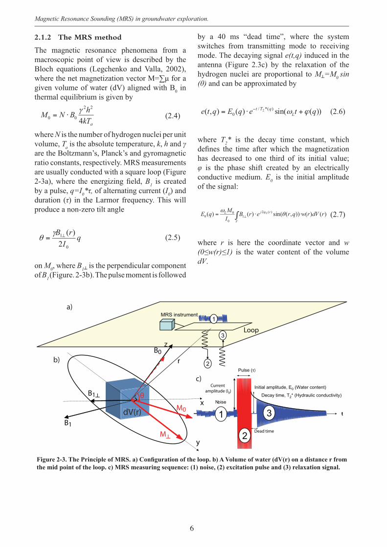
where N is the number of hydrogen nuclei per unit volume, a is the absolute temperature, k, h and are the Boltzmann’s, Planck’s and gyromagnetic ratio constants, respectively. MRS measurements are usually conducted with a square loop (Figure
B1 is created by a pulse, q=I0 of alternating current (I0) and duration ( ) in the Larmor frequency. This will produce a non-zero tilt angle
(2.5)
on M0, where B is the perpendicular component ofB1(Figure. 2-3b). The pulse moment is followed
by a 40 ms “dead time”, where the system switches from transmitting mode to receiving mode. The decaying signal e(t,q) induced in the antenna (Figure 2.3c) by the relaxation of the hydrogen nuclei are proportional to M =M0 sin
and can be approximated by
(2.6)
where 2* is the decay time constant, which
has decreased to one third of its initial value; is the phase shift created by an electrically
conductive medium. E0 is the initial amplitude of the signal:
(2.7)
where r is here the coordinate vector and w is the water content of the volume
dV.
akThBNM
4
22
00
qI
rB
0
1
2)(
))(sin()(),( )(*/0
2 qteqEqte LqTt
)()()),(sin()()( )(21
0
00
0 rdVrwqrerBIMqE
V
rjL
the mid point of the loop. c) MRS measuring sequence: (1) noise, (2) excitation pulse and (3) relaxation signal.
t
esioN
Pulse (τ)
Decay time, T2* (Hydraulic conductivity)
Initial amplitude, E0 (Water content)Current amplitude (I0)
Dead time2
31dV(r)
rB0
x
y
B1
B1┴
a)
b)
c)
M0
M┴
θ
MRS instrument
2
3Loop
1
z
7
METHODS
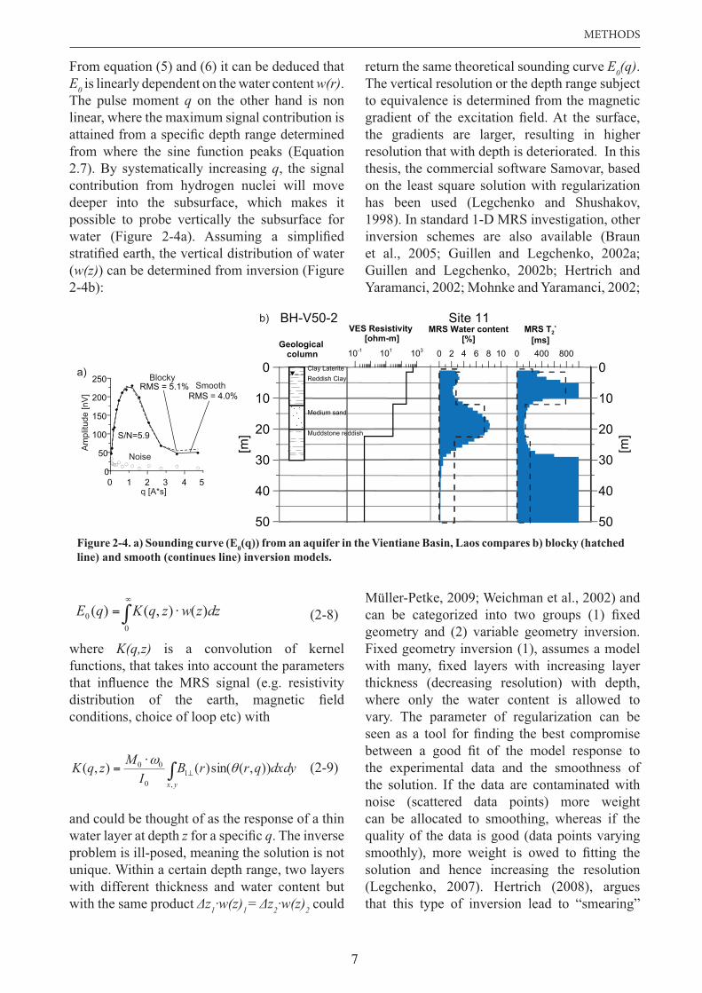
From equation (5) and (6) it can be deduced that E0 is linearly dependent on the water content w(r).The pulse moment q on the other hand is non linear, where the maximum signal contribution is
from where the sine function peaks (Equation 2.7). By systematically increasing q, the signal contribution from hydrogen nuclei will move deeper into the subsurface, which makes it possible to probe vertically the subsurface for
(w(z)) can be determined from inversion (Figure 2-4b):
return the same theoretical sounding curve E0(q).The vertical resolution or the depth range subject to equivalence is determined from the magnetic
the gradients are larger, resulting in higher resolution that with depth is deteriorated. In this thesis, the commercial software Samovar, based on the least square solution with regularization has been used (Legchenko and Shushakov, 1998). In standard 1-D MRS investigation, otherinversion schemes are also available (Braun et al., 2005; Guillen and Legchenko, 2002a; Guillen and Legchenko, 2002b; Hertrich and Yaramanci, 2002; Mohnke and Yaramanci, 2002;
00 )(),()( dzzwzqKqE
yx
dxdyqrrBI
MzqK,
10
00 )),(sin()(),(
Figure 2-4. a) Sounding curve (E0line) and smooth (continues line) inversion models.
50
40
30
20
10
0
[m]
50
40
30
20
10
0
[m]
Clay LateriteReddish Clay
Medium sand
Muddstone reddish
Geologicalcolumn 10-1 101 103
VES Resistivity [ohm-m]
0 2 4 6 8 10
MRS Water content[%]
0 400 800
MRS T2*
[ms]
BH-V50-2 Site 11
a)
0 2 31 4 50
50
100
150
200
250RMS = 5.1%
RMS = 4.0%
S/N=5.9
q [A*s]
Am
plitu
de [n
V]
BlockySmooth
Noise
b)
(2-8)
where K(q,z) is a convolution of kernel functions, that takes into account the parameters
conditions, choice of loop etc) with
(2-9)
and could be thought of as the response of a thin water layer at depth z q. The inverse problem is ill-posed, meaning the solution is not unique. Within a certain depth range, two layers with different thickness and water content but with the same product 1·w(z)1 2·w(z)2 could
Müller-Petke, 2009; Weichman et al., 2002) and
geometry and (2) variable geometry inversion. Fixed geometry inversion (1), assumes a model
thickness (decreasing resolution) with depth, where only the water content is allowed to vary. The parameter of regularization can be
the experimental data and the smoothness of the solution. If the data are contaminated with noise (scattered data points) more weight can be allocated to smoothing, whereas if the quality of the data is good (data points varying
solution and hence increasing the resolution (Legchenko, 2007). Hertrich (2008), argues that this type of inversion lead to “smearing”
8
Magnetic Resonance Sounding (MRS) in groundwater exploration.
of layer boundaries and an overestimation of water content, however no a priori information is needed and aquifers in geological environments with smooth water content variation can be accurately determined. The second scheme (2), assumes a small number of layers, where both water content and layer thickness can vary. Here, prior geological information is necessary and the boundaries between layers are assumed to be sharp rather than smooth. From an interpretation point of view both schemes should be adopted
subsurface aquifer structure and to evaluate the equivalence in the solution (Yaramanci and Hertrich, 2007). Lately, 2-D (Hertrich, 2008) and 3-D (Legchenko et al., 2011; Paper III) inversion schemes have been developed to resolve more complex geological problems. For a more extensive, yet comprehensive review of the mathematical model behind MRS, see Plata and Rubio (2007)and considerations of current MRS models.
2.1.3 Relaxation of the signal
In its simplest acquisition mode, MRS measures the free induction decay constant 2* using a single excitation pulse technique (see section 2.1.2), where several relaxation mechanisms contribute to 2* (Grunewald and Knight, 2011; Keating and Knight, 2008; Kenyon, 1997; Roy et al., 2008):
(2.10)
where 2B, 2S and 2D are the bulk, surface and diffusion relaxation, respectively and the term
0bulk relaxation ( 2B) is the decay time of the bulk water and it is mainly affected by the water molecule interactions and the concentration
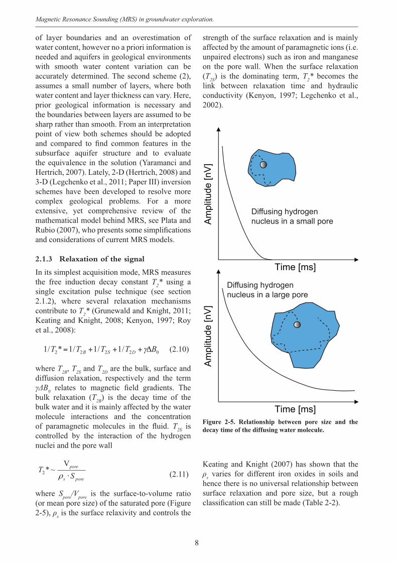
2S is controlled by the interaction of the hydrogen nuclei and the pore wall
(2.11)
where Spore pore is the surface-to-volume ratio (or mean pore size) of the saturated pore (Figure 2-5), s is the surface relaxivity and controls the
strength of the surface relaxation and is mainly affected by the amount of paramagnetic ions (i.e. unpaired electrons) such as iron and manganese on the pore wall. When the surface relaxation ( 2S) is the dominating term, 2* becomes the link between relaxation time and hydraulic conductivity (Kenyon, 1997; Legchenko et al., 2002).
02222 /1/1/1*/1 BTTTT DSB
pores
pore
ST
V~*2
Figure 2-5. Relationship between pore size and the decay time of the diffusing water molecule.
Time [ms]
Am
plitu
de [n
V]
Time [ms]
Am
plitu
de [n
V]Diffusing hydrogen nucleus in a small pore
Diffusing hydrogen nucleus in a large pore
Keating and Knight (2007) has shown that the s varies for different iron oxides in soils and
hence there is no universal relationship between surface relaxation and pore size, but a rough
9
METHODS
The diffusion relaxation ( 2D) is the effect from magnetic gradients on diffusing water molecules. Finally, ( 0) decreases the 2*, which often makes 2*inappropriate to estimate hydraulic properties of the aquifer. Large magnetic gradients could also underestimate the water content (Vouillamoz et al., 2011) and in the worst case reduce the 2*below the threshold of the instrument detection limit (Roy et al., 2008).
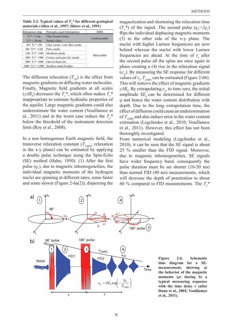
transverse relaxation constant ( 2MRS; relaxation in the x-y plane) can be estimated by applying a double pulse technique using the Spin-Echo (SE) method (Hahn, 1950)pulse (q1), due to magnetic inhomogeneities, the individual magnetic moments of the hydrogen nuclei are spinning at different rates, some faster and some slower (Figure 2-6a(2)), dispersing the
magnetization and shortening the relaxation time ( 2*) of the signal. The second pulse (q2=2q1)
(3) to the other side of the x-y plane. The nuclei with higher Larmor frequencies are now behind whereas the nuclei with lower Larmor frequencies are ahead. At the time of e after the second pulse all the spins are once again in phase creating a (4) rise in the relaxation signal (e ). By measuring the SE response for different values of e, 2MRS can be estimated (Figure 2-6b).This will remove the effect of magnetic gradients
0. By extrapolating e to time zero, the initial amplitude SE0 can be determined for different q and hence the water content distribution with depth. Due to the long extrapolation time, theeffect of diffusion could cause an underestimation of 2MRS and also induce error in the water content estimation (Legchenko et al., 2010; Vouillamoz et al., 2011). However, this effect has not been thoroughly investigated. From numerical modeling (Legchenko et al., 2010), it can be seen that the SE signal is about 25 % smaller than the FID signal. Moreover, due to magnetic inhomogeneities, SE signals have wider frequency band, consequently the pulse duration must be set shorter (10-20 ms) than normal FID (40 ms) measurements, which will decrease the depth of penetration to about 60 % compared to FID measurements. The 2*
Relaxation time Petrophysical Information MRST2* < 3 ms Clay bound waterT2* < 30 ms Sandy clays30< T2* <60 Clay sands, very fine sands60< T2* <120 Fine sands120< T2* <180 Medium sands180< T2* <300 Coarse and gravely sands300< T2* <600 Gravel deposits600< T2* <1500 Surface water bodies
Undetectable
Detectable
Table 2-2. Typical values of T2* for different geological materials (Allen et al., 1997; Shirov et al., 1991)
Figure 2-6. Schematic time diagram for a SE-measurement, showing a) the behavior of the magnetic moments ( ) during b) a typical measuring sequence with the time delay (after
et al., 2011).
a)
Noise
90˚ pulse 180˚ pulse
τ τ
Time
M0
B0
x
z
y
1B0
x
z
y
2B0
x
z
y
x
3
90˚
180˚ pulse
b)1 2
4
3 4
μ μ
μμM
FID1FID2
⎟⎟⎠
⎞⎜⎜⎝
⎛−=
MRS
e
TSEe
202
2exp ττ
SE0
e2τ
T2MRS
10
Magnetic Resonance Sounding (MRS) in groundwater exploration.
can be determined from the width (time) of the spin-echo signal at e multiplied by the factor 0.424. The shorter 2*, the more distinct and narrow SE signal.
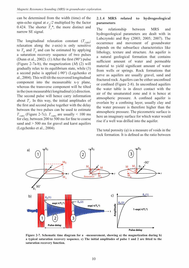
The longitudinal relaxation constant ( 1MRS;relaxation along the z-axis) is only sensitive to B and S and can be estimated by applying a saturation recovery sequence of two pulses (Dunn et al., 2002)(Figure 2-7a-b), the magnetization (M) (2) will gradually relax to its equilibrium state, while (3)
(Legchenko et al., 2004). This will tilt the recovered longitudinal component into the measureable x-y plane, whereas the transverse component will be tilted in the (non measurable) longitudinal (z) direction. The second pulse will hence carry information about 1. In this way, the initial amplitudes of
between the two pulses can be used to estimate 1MRS (Figure 2-7c). 1MRS are usually < 100 ms
sand and > 500 ms for gravel and karst aquifers (Legchenko et al., 2004).
2.1.4 MRS related to hydrogeological parameters
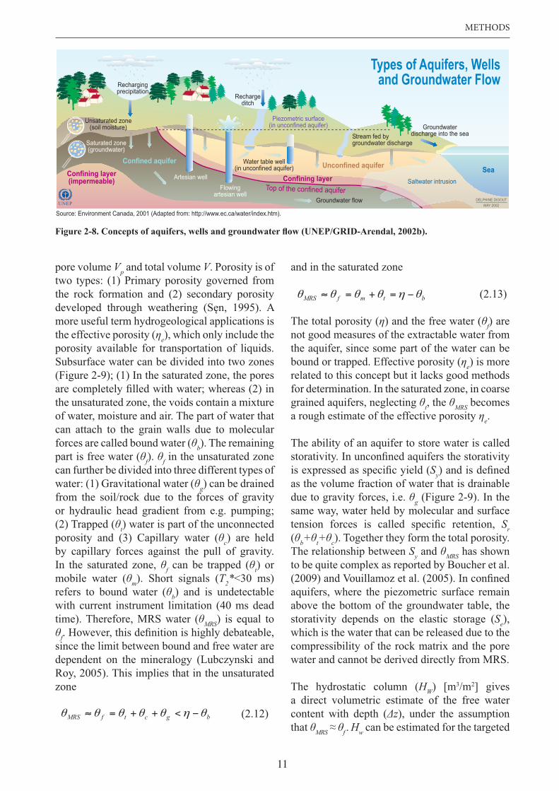
The relationship between MRS and hydrogeological parameters are dealt with inLubczynski and Roy (2003; 2005; 2007). The occurrence and movement of groundwater depends on the subsurface characteristics like lithology, texture and structure. An aquifer is a natural geological formation that contains
from wells or springs. Rock formations that serve as aquifers are usually gravel, sand and
the water table is in direct contact with the air of the unsaturated zone and it is hence at
the water pressure is therefore higher than the atmospheric pressure. The piezometric surface is here an imaginary surface for which water would rise if a well was drilled into the aquifer.
The total porosity ( ) is a measure of voids in the
Figure 2-7. Schematic time diagram for a -measurement, showing a) the magnetization during b)
saturation recovery function.
a)
Am
plit
ude
Pulse delay
E0(1)
E0(2)
1-exp(-t/T1*)
c)
t
E0(1)
E0(2)exp(-t/T2*)exp(-t/T2*)
Pulse delay
b)
M0
M┴
B0
B1
z
y
x
θM
M┴
B0z
y
xMIIM┴
B0
B1
z
y
xM
MII
1 2 3
θ -θ
1 2 3
Relaxation
90˚
-90˚
11
METHODS
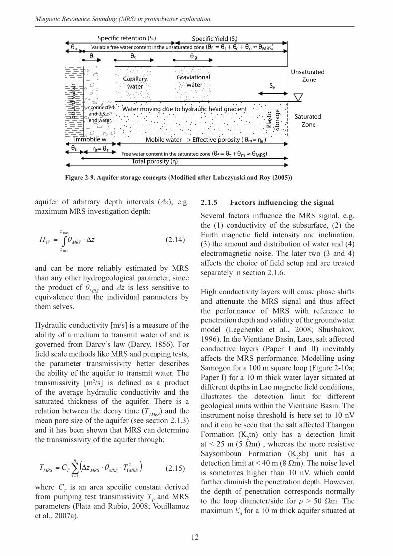
pore volume Vp and total volume V. Porosity is of two types: (1) Primary porosity governed from the rock formation and (2) secondary porosity developed through weathering . A more useful term hydrogeological applications is the effective porosity ( e), which only include the porosity available for transportation of liquids. Subsurface water can be divided into two zones (Figure 2-9); (1) In the saturated zone, the pores
the unsaturated zone, the voids contain a mixture of water, moisture and air. The part of water that can attach to the grain walls due to molecular forces are called bound water ( b). The remaining part is free water ( f). f in the unsaturated zone can further be divided into three different types of water: (1) Gravitational water ( g) can be drained from the soil/rock due to the forces of gravity or hydraulic head gradient from e.g. pumping; (2) Trapped ( t) water is part of the unconnected porosity and (3) Capillary water ( c) are held by capillary forces against the pull of gravity. In the saturated zone, f can be trapped ( t) or mobile water ( m). Short signals ( 2*<30 ms) refers to bound water ( b) and is undetectable with current instrument limitation (40 ms dead time). Therefore, MRS water ( MRS) is equal to
fsince the limit between bound and free water are dependent on the mineralogy (Lubczynski and Roy, 2005). This implies that in the unsaturated zone
(2.12)
and in the saturated zone
(2.13)
The total porosity ( ) and the free water ( f) are not good measures of the extractable water from the aquifer, since some part of the water can be bound or trapped. Effective porosity ( e) is more related to this concept but it lacks good methods for determination. In the saturated zone, in coarse grained aquifers, neglecting t, the MRS becomes a rough estimate of the effective porosity e.
The ability of an aquifer to store water is called
Syas the volume fraction of water that is drainable due to gravity forces, i.e. g (Figure 2-9). In the same way, water held by molecular and surface
Sr( b t c). Together they form the total porosity. The relationship between Sy and MRS has shown to be quite complex as reported by Boucher et al.(2009) and Vouillamoz et al. (2005)aquifers, where the piezometric surface remain above the bottom of the groundwater table, the storativity depends on the elastic storage (Se),which is the water that can be released due to the compressibility of the rock matrix and the pore water and cannot be derived directly from MRS.
The hydrostatic column (HW) [m3/m2] gives a direct volumetric estimate of the free water content with depth ( ), under the assumption that MRS f . Hw can be estimated for the targeted
MAY 2002DELPHINE DIGOUT
Artesian wellFlowing
artesian well
Water table well(in unconfined aquifer)
Confined aquifer Unconfined aquifer
Piezometric surface(in unconfined aquifer)
Saltwater intrusion
Rechargingprecipitation
Rechargeditch
Stream fed bygroundwater discharge
Unsaturated zone(soil moisture)
Confining layer(impermeable) Confining layer
Groundwaterdischarge into the sea
Sea
Groundwater flow
Saturated zone(groundwater)
Types of Aquifers, Wellsand Groundwater Flow
Top of the confined aquifer
Source: Environment Canada, 2001 (Adapted from: http://www.ec.ca/water/index.htm).UNEP
bgctfMRS
btmfMRS
12
Magnetic Resonance Sounding (MRS) in groundwater exploration.
aquifer of arbitrary depth intervals ( ), e.g. maximum MRS investigation depth:
(2.14)
and can be more reliably estimated by MRS than any other hydrogeological parameter, since the product of MRS and is less sensitive to equivalence than the individual parameters by them selves.
Hydraulic conductivity [m/s] is a measure of the ability of a medium to transmit water of and is governed from Darcy’s law (Darcy, 1856). For
the parameter transmissivity better describes the ability of the aquifer to transmit water. The transmissivity [m2
of the average hydraulic conductivity and the saturated thickness of the aquifer. There is a relation between the decay time ( 1MRS) and the mean pore size of the aquifer (see section 2.1.3) and it has been shown that MRS can determine the transmissivity of the aquifer through:
(2.15)
where Cfrom pumping test transmissivity P and MRS parameters (Plata and Rubio, 2008; Vouillamoz et al., 2007a).
2.1.5 Factors influencing the signal
the (1) conductivity of the subsurface, (2) the
(3) the amount and distribution of water and (4) electromagnetic noise. The later two (3 and 4)
separately in section 2.1.6.
High conductivity layers will cause phase shifts and attenuate the MRS signal and thus affect the performance of MRS with reference to penetration depth and validity of the groundwater model (Legchenko et al., 2008; Shushakov, 1996). In the Vientiane Basin, Laos, salt affected conductive layers (Paper I and II) inevitably affects the MRS performance. Modelling using Samogon for a 100 m square loop (Figure 2-10a; Paper I) for a 10 m thick water layer situated at
illustrates the detection limit for different geological units within the Vientiane Basin. The instrument noise threshold is here set to 10 nV and it can be seen that the salt affected Thangon Formation (K2tn) only has a detection limit
Saysomboun Formation (K2sb) unit has a
is sometimes higher than 10 nV, which could further diminish the penetration depth. However, the depth of penetration corresponds normally to the loop diameter/side for maximum E0 for a 10 m thick aquifer situated at
Water moving due to hydraulic head gradient
Capillary water
Graviational water
Unconnected and dead end water
Unsaturated Zone
Saturated Zone
Boun
d w
ater
Ela
stic
St
orag
e
Specific retention (S ) Specific Yield (S )
Total porosity (η)Free water content in the saturated zone (θf = θt + θm ≈ θMRS)
S
θθθθ
θImmobile w. Mobile water --> Effective porosity ( θ = η )
η = θ
Variable free water content in the unsaturated zone (θf = θt + θc + θg ≈ θMRS) b
b
em
t
tt
c g
r y
e
max
min
z
zMRSW zH
n
iMRSMRSMRSTMRS TzCT
1
21
13
METHODS
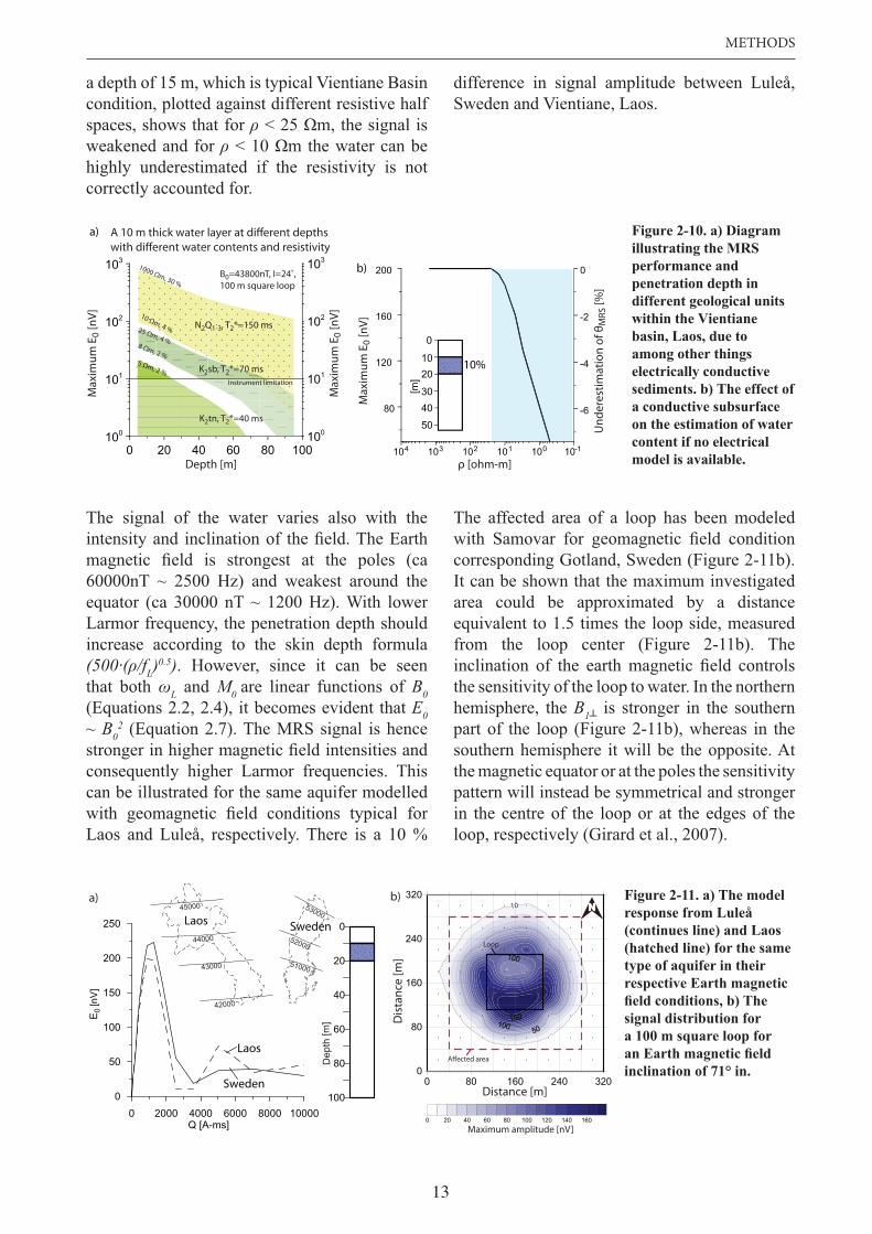
a depth of 15 m, which is typical Vientiane Basin condition, plotted against different resistive half spaces, shows that for weakened and for highly underestimated if the resistivity is not correctly accounted for.
difference in signal amplitude between Luleå, Sweden and Vientiane, Laos.
Figure 2-10. a) Diagram illustrating the MRS performance and penetration depth in different geological units
basin, Laos, due to among other things electrically conductive sediments. b) The effect of a conductive subsurface on the estimation of water content if no electrical model is available.
The signal of the water varies also with the
60000nT ~ 2500 Hz) and weakest around the equator (ca 30000 nT ~ 1200 Hz). With lower Larmor frequency, the penetration depth should increase according to the skin depth formula
L)0.5). However, since it can be seen that both L and M0 are linear functions of B0(Equations 2.2, 2.4), it becomes evident that E0~ B0
2 (Equation 2.7). The MRS signal is hence
consequently higher Larmor frequencies. This can be illustrated for the same aquifer modelled
Laos and Luleå, respectively. There is a 10 %
The affected area of a loop has been modeled
corresponding Gotland, Sweden (Figure 2-11b). It can be shown that the maximum investigated area could be approximated by a distance equivalent to 1.5 times the loop side, measured from the loop center (Figure 2-11b). The
the sensitivity of the loop to water. In the northern hemisphere, the B is stronger in the southern part of the loop (Figure 2-11b), whereas in the southern hemisphere it will be the opposite. At the magnetic equator or at the poles the sensitivity pattern will instead be symmetrical and stronger in the centre of the loop or at the edges of the loop, respectively (Girard et al., 2007).
0 20 40 60 80 100100
101
102
103
100
101
102
103
Depth [m]
N2Q1-3, T2*=150 ms
K2sb, T2*=70 ms
K2tn, T2*=40 ms
1000 Ωm, 30 %
10 Ωm, 4 %25 Ωm, 4 %8 Ωm, 2 %5 Ωm, 2 %
Instrument limitation
B0=43800nT, I=24˚,100 m square loop
A 10 m thick water layer at different depthswith different water contents and resistivity
Max
imum
E 0 [n
V]
Max
imum
E 0 [n
V]
a)
40
20
0
[m]
10
30
50
104 103 102 101 100 10-1
80
120
160
200
-6
-4
-2
0
ρ [ohm-m]
Max
imum
E 0 [n
V]
Und
eres
timat
ion
of θ
MRS
[%]
b)
10%
Laos Sweden
51000
52000
53000
44000
45000
43000
42000
0 2000 4000 6000 8000 10000Q [A-ms]
0
50
100
150
200
250
100
80
60
40
20
0
Dep
th [m
]
Laos
Sweden
a)
0 80 160 240 3200
80
160
240
320
0 20 40 60 80 100 120 140 160
Dis
tanc
e [m
]
Distance [m]
10 N
Maximum amplitude [nV]
Affected area
Loop
b)
E0
[nV
]
Figure 2-11. a) The model response from Luleå (continues line) and Laos (hatched line) for the same type of aquifer in their respective Earth magnetic
signal distribution for a 100 m square loop for
inclination of 71° in.
14
Magnetic Resonance Sounding (MRS) in groundwater exploration.
2.1.6 Instrument and fieldwork
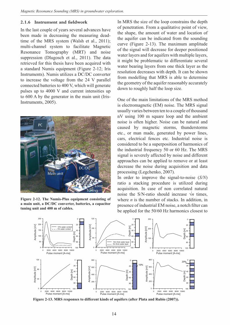
In the last couple of years several advances have been made in decreasing the measuring dead-time of the MRS system (Walsh et al., 2011);multi-channel system to facilitate Magnetic Resonance Tomography (MRT) and noise suppression (Dlugosch et al., 2011). The data retrieved for this thesis have been acquired with a standard Numis equipment (Figure 2-12; Iris Instruments). Numis utilizes a DC/DC converter to increase the voltage from the 24 V parallel connected batteries to 400 V, which will generate pulses up to 4000 V and current intensities up to 600 A by the generator in the main unit (Iris-Instruments, 2005).
In MRS the size of the loop constrains the depth of penetration. From a qualitative point of view, the shape, the amount of water and location of the aquifer can be indicated from the sounding curve (Figure 2-13). The maximum amplitude of the signal will decrease for deeper positioned water layers and for aquifers with multiple layers, it might be problematic to differentiate several water bearing layers from one thick layer as the resolution decreases with depth. It can be shown from modelling that MRS is able to determine the geometry of the aquifer reasonably accurately down to roughly half the loop size.
One of the main limitations of the MRS method is electromagnetic (EM) noise. The MRS signal usually varies between ten to a couple of thousand nV using 100 m square loop and the ambient noise is often higher. Noise can be natural and caused by magnetic storms, thunderstorms etc., or man made, generated by power lines, cars, electrical fences etc. Industrial noise is considered to be a superposition of harmonics of the industrial frequency 50 or 60 Hz. The MRS signal is severely affected by noise and different approaches can be applied to remove or at least decrease the noise during acquisition and data processing (Legchenko, 2007).In order to improve the signal-to-noise ( )ratio a stacking procedure is utilized during acquisition. In case of non correlated natural noise the S/N-ratio should increase times, where n is the number of stacks. In addition, in
be applied for the 50/60 Hz harmonics closest to
Figure 2-12. The Numis-Plus equipment consisting of a main unit, a DC/DC converter, batteries, a capacitor tuning unit and 400 m of cables.
0 2000 4000 6000 8000 100000
50
100
150
200
250
100
80
60
40
20
0
10% water content5% water content
Am
plitu
de [n
V]
Pulse moment [A-ms]
Dep
th [m
]
0 2000 4000 6000 8000 100000
40
80
120
100
80
60
40
20
0
10m thick water layer5m thick water layer
Am
plitu
de [n
V]
Pulse moment [A-ms]
Dep
th [m
]
0 2000 4000 6000 8000 100000
100
200
300
100
80
60
40
20
0
Am
plitu
de [n
V]
Pulse moment [A-ms]
Dep
th [m
]
0 2000 4000 6000 8000 100000
40
80
120
100
80
60
40
20
0
Am
plitu
de [n
V]
Pulse moment [A-ms]
Dep
th [m
]
0 2000 4000 6000 8000 100000
200
400
600
800
100
80
60
40
20
020%
Am
plitu
de [n
V]
Pulse moment [A-ms]
Dep
th [m
]
0 2000 4000 6000 8000 100000
200
400
600
800
100
80
60
40
20
0
10%
Am
plitu
de [n
V]
Pulse moment [A-ms]
Dep
th [m
]
15
METHODS
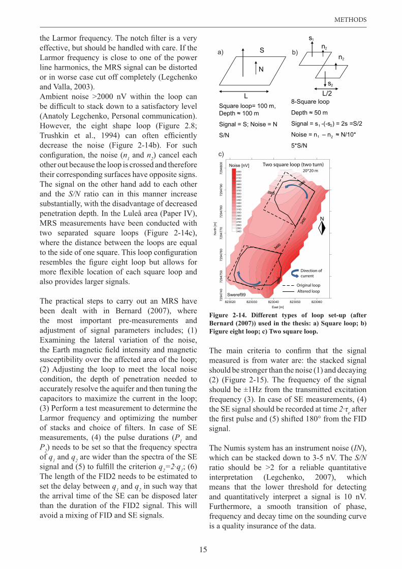
effective, but should be handled with care. If the Larmor frequency is close to one of the power line harmonics, the MRS signal can be distorted or in worse case cut off completely (Legchenkoand Valla, 2003).Ambient noise >2000 nV within the loop can
(Anatoly Legchenko, Personal communication). However, the eight shape loop (Figure 2.8;
decrease the noise (Figure 2-14b). For such n1 and n2) cancel each
other out because the loop is crossed and therefore their corresponding surfaces have opposite signs. The signal on the other hand add to each other and the ratio can in this manner increase substantially, with the disadvantage of decreased penetration depth. In the Luleå area (Paper IV), MRS measurements have been conducted with two separated square loops (Figure 2-14c), where the distance between the loops are equal
also provides larger signals.
The practical steps to carry out an MRS have been dealt with in Bernard (2007), where the most important pre-measurements and adjustment of signal parameters includes; (1) Examining the lateral variation of the noise,
susceptibility over the affected area of the loop; (2) Adjusting the loop to meet the local noise condition, the depth of penetration needed to accurately resolve the aquifer and then tuning the capacitors to maximize the current in the loop; (3) Perform a test measurement to determine the Larmor frequency and optimizing the number
measurements, (4) the pulse durations (P1 and P2) needs to be set so that the frequency spectra of q1 and q2 are wider than the spectra of the SE
q2=2.q1; (6) The length of the FID2 needs to be estimated to set the delay between q1 and q2 in such way that the arrival time of the SE can be disposed later than the duration of the FID2 signal. This will avoid a mixing of FID and SE signals.
measured is from water are: the stacked signal should be stronger than the noise (1) and decaying (2) (Figure 2-15). The frequency of the signal should be ±1Hz from the transmitted excitation frequency (3). In case of SE measurements, (4) the SE signal should be recorded at time 2 e after
signal.
The Numis system has an instrument noise (IN),which can be stacked down to 3-5 nV. The ratio should be >2 for a reliable quantitative interpretation (Legchenko, 2007), which means that the lower threshold for detecting and quantitatively interpret a signal is 10 nV. Furthermore, a smooth transition of phase, frequency and decay time on the sounding curve is a quality insurance of the data.
Figure 2-14. Different types of loop set-up (after
Figure eight loop; c) Two square loop.
S
N
L
s1
s2
n2
n2
L/2
Square loop= 100 m,Depth ≈ 100 m
Signal = S; Noise = N
S/N
8-Square loop
Depth ≈ 50 m
Signal = s -(-s ) = 2s =S/2
Noise = n – n ≈ N/10*
5*S/N21
1 2
Noise [nV]
823020 823030 823040 823050 823060East [m]
7294
740
7294
750
7294
760
7294
770
7294
780
7294
790
7294
800
Nor
th [m
]
24002500260027002800290030003100320033003400350036003700380039004000410042004300
Original loop Altered loop
N
Direction of current
Two square loop (two turn) 20*20 m
Sweref99
a) b)
c)
16
Magnetic Resonance Sounding (MRS) in groundwater exploration.
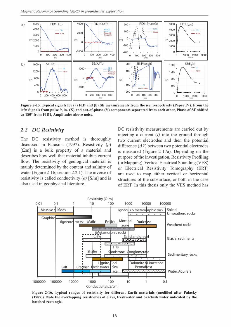
2.2 DC Resistivity
The DC resistivity method is thoroughly discussed in Parasnis (1997). Resistivity ( )
describes how well that material inhibits current
mainly determined by the content and salinity of water (Figure 2-16; section 2.2.1). The inverse of resistivity is called conductivity ( [S/m] and is also used in geophysical literature.
DC resistivity measurements are carried out by injecting a current (I) into the ground through two current electrodes and then the potential difference ( ) between two potential electrodes is measured (Figure 2-17a). Depending on the
(or Mapping), Vertical Electrical Sounding (VES) or Electrical Resistivity Tomography (ERT) are used to map either vertical or horizontal structures of the subsurface, or both in the case of ERT. In this thesis only the VES method has
[ms]
[nV]
FID1
Noise
FID1: E(t)
0 100 200 300 4000
1000
2000
3000
4000
5000
[ms]
[nV]
FID1(X)FID1(Y)Noise (X)Noise (Y)
FID1: X,Y(t)
0 100 200 300 400-2000
0
2000
4000
[A*ms]
[nV]
FID1
Noise
FID1:E0(q)
0 1000 2000 30000
1000
2000
3000
4000
5000
[ms]
[nV]
SE
Noise
SE: E(t)
0 200 400 600 8000
400
800
1200
1600
[ms]
[nV]
SE(X)SE(Y)Noise (X)Noise (Y)
SE: X,Y(t)
0 200 400 600 800
-1000
0
1000
[ms]
[nV]
SE
Noise
SE: Phase(t)
0 200 400 600 800-200
-100
0
100
200SE
Noise
[ms]
[nV]
SE:E0(q)
[ms]
[nV]
FID1
Noise
FID1: Phase(t)
0 100 200 300 400-200
-100
0
100
200a)
b)
0 1000 2000 30000
400
800
1200
1600
left: Signals from pulse 9, in- (X) and out-of-phase (Y) components separated from each other, Phase of SE shifted ca 180° from FID1, Amplitudes above noise.
0.01 0.1 1 10 100 1000 10000 100000Resistivity [Ω-m]
Conductivity[μS/cm]100000 10000 1000 100 10 1 0.11000000
Massive sulfides
Graphite
Igneous & metamorphic rock
Salt Brackish Fresh water PermafrostSeaice
Shales Sandstone ConglomerateTills
Sand and gravelClay
(Igneous rocks: Mafic Felsic)
(Metamorphic rock)
Mottledzone
Duricrust
ShieldUnweatherd rocks
Weatherd rocks
Glacial sediments
Sedimentary rocks
Water, Aquifers
Lignite, Coal Dolomite &Limestone
hatched rectangle.
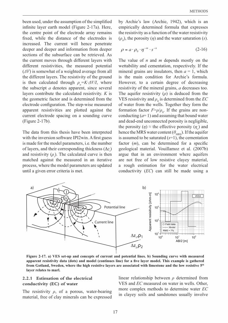
17
METHODS
the centre point of the electrode array remains
increased. The current will hence penetrate deeper and deeper and information from deeper sections of the subsurface can be retrieved. As the current moves through different layers with different resistivities, the measured potential ( ) is somewhat of a weighted average from all the different layers. The resistivity of the ground is then calculated through a , where the subscript a denotes apparent, since several layers contribute the calculated resistivity. K is the geometric factor and is determined from the
apparent resistivities are plotted against the current electrode spacing on a sounding curve (Figure 2-17b).
The data from this thesis have been interpreted
is made for the model parameters, i.e. the number of layers, and their corresponding thickness ( zi)and resistivity ( i). The calculated curve is then matched against the measured in an iterative process, where the model parameters are updated until a given error criteria is met.
by Archie’s law (Archie, 1942), which is an empirically determined formula that expresses the resistivity as a function of the water resistivity ( 0), the porosity ( ) and the water saturation (s).
(2-16)
The value of n and m depends mostly on the wettability and cementation, respectively. If the mineral grains are insulators, then a = 1, which is the main condition for Archie’s formula. However, to a certain degree of decreasing resistivity of the mineral grains, a decreases too. The aquifer resistivity ( ) is deduced from the VES resistivity and 0 is determined from the ECof water from the wells. Together they form the formation factor F= / 0. If the grains are non-conducting (a= 1) and assuming that bound water and dead-end unconnected porosity is negligible, the porosity ( e) and hence the MRS water content ( MRS). If the aquifer is assumed to be saturated (s=1), the cementation factor (mgeological material. Vouillamoz et al. (2007b) argue that in an environment where aquifers are not free of low resistive clayey material, a rough estimation for the water electrical conductivity (EC) can still be made using a
Δz1,ρ1
Δz2,ρ2
Current line
Potential line
IΔV
100 101 102
AB/2 [m]
101
102
103
104
App
aren
t res
isiti
vity
[ohm
-m]
VES3
Field data
RMS = 7%Model
a) b)
from Gotland, Sweden, where the high resistive layers are associated with limestone and the low resistive 5th
layer relates to marl.
2.2.1 Estimation of the electrical conductivity (EC) of water
The resistivity , of a porous, water-bearing material, free of clay minerals can be expressed
nm sa 0
linear relationship between determined from VES and EC measured on water in wells. Other, more complex methods to determine water ECin clayey soils and sandstones usually involve
18
Magnetic Resonance Sounding (MRS) in groundwater exploration.
determination of the cation exchange capacity (obtained in laboratory), which is not always
dependent on the concentration and mobility of ions, where mobility is highly temperature dependent. Conductivity measurements of water are usually standardized for a temperature
aquifer conductivity it is therefore important to correct for the true temperature of the water. The conductivity of most groundwater varies with about 2% per °C (Clesceri et al., 1998).
2.2.2 Water quality parameters related to EC of water
Salinity is measured in Total Dissolved Solids ( ), which is the total sum of cations and anions and the undissociated dissolved species
however, can also be determined by multiplying the electrical conductivity (EC
C ). The C
n available water samples, where and EChave been determined:
(2-17)
The C depends upon the types of salt present, i.e. the concentration and mobility of the different constituents, which makes it vary between 0.55-0.90 for normal groundwater (Reynolds and Richards, 1996). The C increases with higher concentration of ions, since their activity is reduced when they are more densely assembled and hence their ability to conduct current. Poorly dissociated calcium and sulphate ions will also increase the C . is often used for evaluating the water quality for domestic usage. Water with
lower than 600 mg/l is considered to be of good quality (WHO, 1996).
The salt content is sometimes measured with reference to the level of chloride, which can also be directly related to EC. According to the Swedish Environmental Protection Agency (SEPA), chloride concentrations >100 mg/l can have a corrosive effect on metal pipes and concentrations >300 mg/l can cause taste
differences (SEPA, 2000). The major source of natural chloride in groundwater comes from dissolution of halite.
Water with a high mineral content (>150 mg/l as CaHCO3; WHO, 1996), primarily of calcium (Ca2+) and magnesium (Mg2+) ions, is considered as hard. Hardness of water is an important criterion for technical and esthetical reasons. Hard water can be expected in regions with large amounts of limestone (CaCO3) or dolomite (CaMg(CO3)2) (Reynolds and Richards, 1996). Hardness of the water with its polyvalent ions directly contributes to conductivity (Krawczyk and Ford, 2006; 2007). The total hardness (H )can be calculated from the Ca2+ and Mg2+ content in the water from H 3] = 2.497 [Ca2+ 2+ as described in Standard Methods 2340 B (Clesceri et al., 1998).
The amount of salts and especially sodium plays a vital role in judging the salinity hazard for crops and plants. Many plants are sensitive to high salinity and when the concentration of sodium (Na+) is high, it tends to be absorbed by clay particles, while replacing Ca2+ and Mg2+.This exchange process reduces soil permeability and could result in poor internal drainage and hard, infertile soils (US Salinity Laboratory Staff, 1954). The sodium hazard of irrigation water is estimated by the Sodium Absorption Ratio: SAR=Na+ 2++Mg2+ and relates to the relative proportions of Na+, Ca2+ and Mg2+
content. SAR and EC are usually plotted together in a US Salinity Laboratory diagram to categorize and evaluate the usability of different water.
2.3 Radiomagnetotelluric (RMT)
The RMT (Radiomagnetotelluric) method makes use of the signal in the frequency range between 15-250 kHz from long-distance radio transmitters. Induction of currents in the ground
the tensor RMT technique, two horizontal
simultaneously. The ratio between the horizontal
frequency are directly related to the resistivity of the ground. The signal at lower frequencies
n
i
n
iTDS cmSEClmgTDSC
11///
19
METHODS
penetrates deeper into the subsurface and the variation of resistivity with depth can thus be determined.
then transformed into resistivity and phase at each frequency and station. The processing of the RMT data, is made with a band averaging technique (Bastani, 2001), where 8 frequencies from 14 to 226 kHz are used for the 2D-inversion. Tof Rebocc, Occam type, based on smoothing through regularization (Kalscheuer et al., 2008; Siripunvaraporn and Egbert, 2000). The RMT data were acquired with the EnviroMT system (Paper III), developed at Uppsala University (Bastani, 2001) and processed by Lena Persson, the Geological Survey of Sweden (SGU).
2.4 Ground Penetrating Radar (GPR)
Ground Penetrating Radar (GPR) is an
continues short electromagnetic pulses are transmitted into the ground and part of
boundaries or buried objects. The propagation of the radar waves depend on the electrical properties of the ground. The attenuation of the radar wave is primarily controlled by electrical conductivity, whereas the velocity depends on the dielectric constant ( ), which in turn is highly
Differences in between rock strata and objects
processed and displayed against the two-way travel time in a radargram. GPR antennas for geological applications are normally in the range of 10 to 1000 MHz. The choice of antenna is a compromise between resolution and penetration depth. High frequency antennas, i.e. short wave lengths provide higher resolution, but due to higher absorption and scattering, have inferior penetration depth.
In this thesis the Ramac GPR system from Malå Geoscience has been used with a 250 MHz shielded antenna (Paper III and IV). Data were collected with the common offset method, in which the transmitting and receiving antennas
the signal-to-noise ratio, stacking were applied and a “hip chain” was used to measure the
the data included “time zero” shift, amplitude
2.5 Complex resistivity (CR; In laboratory)
With the complex resistivity (CR)/spectral induced polarization (SIP) method the resistivity and phase for a range of frequencies can be measured. The IP phenomena are believed to have two origins. (1) The electrical conduction in most rocks are electrolytic (ions in pore water), but when metallic minerals are blocking the pore path, the ions are hindered. This leads to an accumulation of charges along the grain, resulting in an increase of electro chemical potential over the metallic grain. When the current is turned off, the ions are dispersed leading to a slowly decaying potential (Electrode polarization). (2) Clay bearing minerals can
usually have a negative net charge, positive ions are attracted to pore boundary, resulting in a blocking of ions in narrow passages (Membrane polarization).The CR instrument used in this study (Paper I and III) has been developed at the petrophysical laboratory in Luleå University of Technology and measures the resistivity and phase for frequencies varying between 0.1 and 30 Hz against a reference resistance that can be varied between 2, 10, 100 and 1000 k for both cylindrical and cubic rock samples. The data has
1978):
(2-18)
using a Monte Carlo inversion scheme in MathCAD developed by Hans Thunehed (Triumf et al., 2000), where is the resistivity at the frequency , is the DC resistivity and mc, t and c are the chargeability, time constant and shape factor, respectively. The chargeability and the time constant has shown to be correlated to the clay content and hydraulic conductivity of the rock, respectively (Pelton et al., 1978).
cimc )(1
111)(t
20
Magnetic Resonance Sounding (MRS) in groundwater exploration.
3 MAIN RESULTS AND CONCLUSIONS
A summary of the research from papers I and II (Vientiane Basin in Laos (section 3.1)), papers III (Gotland, Sweden (section 3.2)) and paper IV (Luleå; Sweden (section 3.3)) is here presented and will be discussed in the sections below.
3.1 Vientiane Basin, Laos
Most Lao people lives in rural parts of the country and are heavily dependent on dug wells, river and rain water as their main water source (Medlicott, 2001). Due to a high morbidity rate
of domestic waste and excreta from farm animals, the “Project for Groundwater Development in Vientiane Province” was implemented by Japan International Cooperation Agency (JICA). This project aimed at raising the water supply ratio in the rural areas by drilling deep wells (JICA, 1993). In total, 118 deep wells were drilled and when evaluating the project in year 2000, as much as 60 % of the wells were not used for drinking due to bad water quality or maintenance problem (JICA, 2000). The bad water quality was partially due to salt in the groundwater. Rock salt is naturally occurring within the basin in the Thangon Formation, at depths as shallow as at 50 m (Long et al., 1986). The Vertical Electrical Sounding (VES) technique has widely been used to characterize aquifers and detect salt groundwater since there is a direct relationship between the amount and salinity of water and the resistivity of a geological material. However, using only VES, it is not possible to distinguish high conductive groundwater from e.g. increased clay content (Figure 2-16). By combining MRS
characterize the different geological units within the Vientiane Basin; To distinguish freshwater aquifers from clay and salt affected groundwater; Moreover, explore the possibility to determine water quality parameters, such as Total Dissolved Solids (TDS), chloride and hardness, directly from geophysical parameters.
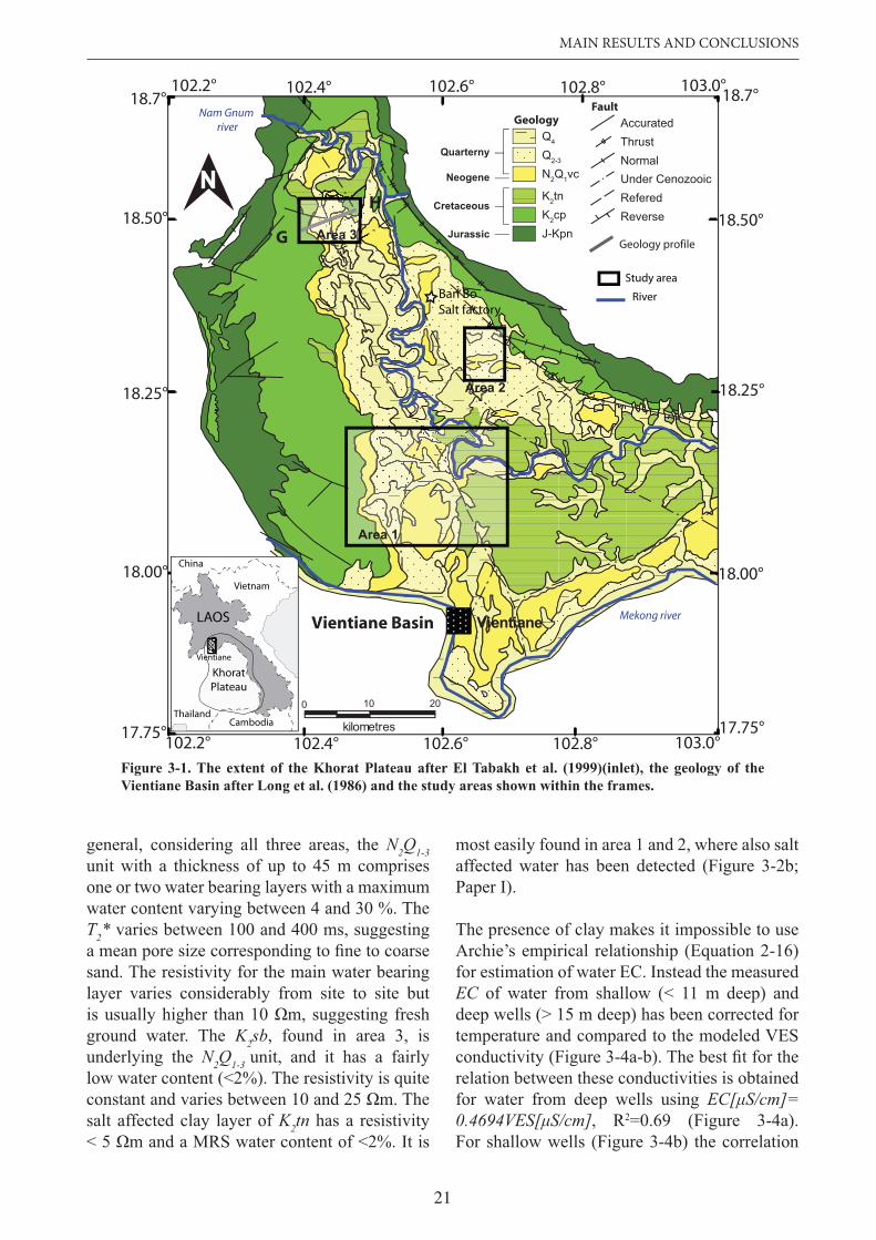
The Vientiane Basin is located in the very northern part of the Khorat Plateau (Figure 3-1, inlet map). During the Cretaceous, due to
relative sea-level rise, the plateau underwent
isolated from the oceans. This created the Thangon Formation (K2tn; > 550 m), a unit with three salt layer separated by red-colored
K2tn isoverlain by the Saysomboun Formation (K2sb;<150 m). This formation originates from upper Cretaceous and is composed of red-brown clay-stone that gradually changes to siltstone, which in turn is overlain by the Vientiane Formation (N2Q1-2) (<70 m) of Neogene to Quaternary origin and the stratigraphic units Q2-3 (<25 m) and Q4 (<0.5 m thick) of Quaternary origin. The Vientiane Formation and the Q2-3 unit have similar geological characteristics and will be treated as one stratigraphic unit (N2Q1-3) in this study. The N2Q1-3 is of alluvial origin and it is mainly composed of gravel, sand and clay. The
is regarded as high. Underlying the Thangon Formation is the Khorat Group, consisting of formations largely composed of sandstone of Cretaceous and Jurassic age.
3.1.1 Main results
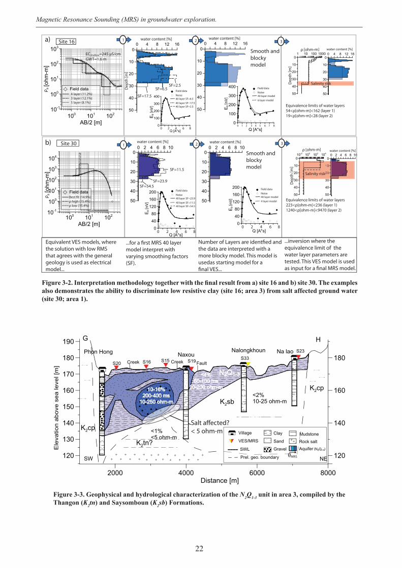
Data were collected from three areas (Figure 3-1). However, the measurements were concentrated to area 3, since it holds the majority of drilled deep wells. All together, 32 MRS and 39 VES were conducted together with 38 water samples collected from both shallow and deep wells. Where MRS and/or VES were performed close to boreholes with geological logging data, that data have been used to constrain the models. MRS and VES data have also been interpreted
better evaluate the equivalence (Figure 3-2) and the risk of salinisation.
The different geological units have been characterized according to water content, decay time ( 2*) (Table 2-2) and resistivity in all three areas. In the N2Q1-3 unit MRS has shown
(high content of water) and penetration depth (Figure 2-10a). The geological cross section GH compiled from borehole data (JICA, 1994) and MRS and VES data, illustrates the soil and rock characteristics of the area 3 (Figure 3-3). In
21
MAIN RESULTS AND CONCLUSIONS
general, considering all three areas, the N2Q1-3unit with a thickness of up to 45 m comprises one or two water bearing layers with a maximum water content varying between 4 and 30 %. The
2* varies between 100 and 400 ms, suggesting
sand. The resistivity for the main water bearing layer varies considerably from site to site but
ground water. The K2sb, found in area 3, is underlying the N2Q1-3 unit, and it has a fairly low water content (<2%). The resistivity is quite
salt affected clay layer of K2tn has a resistivity
most easily found in area 1 and 2, where also salt affected water has been detected (Figure 3-2b; Paper I).
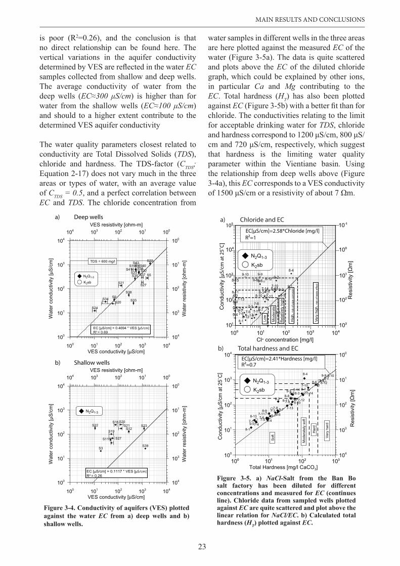
The presence of clay makes it impossible to use Archie’s empirical relationship (Equation 2-16) for estimation of water EC. Instead the measured EC of water from shallow (< 11 m deep) and deep wells (> 15 m deep) has been corrected for temperature and compared to the modeled VES
relation between these conductivities is obtained for water from deep wells using
, R2=0.69 (Figure 3-4a). For shallow wells (Figure 3-4b) the correlation
kilometres
0 10 20
Vientiane Basin
H
G
102.6° 102.8°102.4°102.2° 103.0°17.75°
18.25°
18.00°
18.50°
18.7°
Area 2
China
Vietnam
Thailand
LAOS
Vientiane
Cambodia
KhoratPlateau
GeologyFault
Geology profile
Quarterny
Neogene
Cretaceous
Jurassic
Q4
Q2-3
N2Q1vc
K2tnK2cpJ-Kpn
AccuratedThrustNormalUnder CenozooicReferedReverse
N
17.75°
18.25°
18.7°
18.00°
18.50°
102.8°102.4°
Mekong river
Nam Gnum river
Ban BoSalt factory
Area 3
Area 2
Area 1
Vientiane
River
Study area
102.6°102.2° 103.0°
22
Magnetic Resonance Sounding (MRS) in groundwater exploration.
0 2 4 6 8 10
50
40
30
20
10
0
water content [%]
100 101 102
AB/2 [m]
10-1
100
101
102
103
104
[ohm
-m]
ρ a Field data Best fit (14.9%)ρ high (15.4%)ρ low (15.4%)
Site 300 2 4 6 8 10
50
40
30
20
10
0
water content [%]0 2 4 6 8 10
50
40
30
20
10
0
water content [%]
0
1 2 3
10-2 100 102 104
50
40
30
20
10
0
ρ [ohm-m]
Dep
th [m
]
20
10
30
Salinity risk
0 2 4 6 8Q [A*s]
0
40
80
120
160
200
E0 [
nV]
Field dataNoise40 layer model4 layer model
Q [A*s]0
40
80
120
160
200
0 2 4 6 8
E0 [
nV]
Field dataNoise40 layer SF=23.940 layer SF=11.540 layer SF=54.5
100 101 102
AB/2 [m]
10-1
100
101
102
103[o
hm-m
]ρ a Field data
4 layer (11.2%)3 layer (12.1%)5 layer (8.1%)
Site 16
Dep
th [m
]
0 4 8 12 16
50
40
30
20
10
0
water content [%]water content [%]0 4 8 12 16
50
40
30
20
10
0
SF=2.5SF=6.5
SF=17.5
Q
E0 [
nV]
[A*s]0
100
200
300
400 Field dataNoise40 layer model6 layer model
0 1 2 3 4 5 6 7 8
1 2 3
Equivalent VES models, where the solution with low RMS that agrees with the general geology is used as electricalmodel...
...for a first MRS 40 layermodel interpret with varying smoothing factors(SF).
Number of Layers are identfied and the data are interpreted with a more blocky model. This model is usedas starting model for a final VES...
...inversion where the equivalence limit of the water layer parameters are tested. This VES model is used as input for a final MRS model.
ECshallow=245 μS/cmGWT=1.6 m
1 10 100 1000
50
40
30
20
10
0
Equivalence limits of water layers54<ρ[ohm-m]<162 (layer 1)19<ρ[ohm-m]<28 (layer 2)
ρ [ohm-m]
Dep
th [m
]
0 4 8 12 16
50
40
30
20
10
0
water content [%]
40Salinity risk
Equivalence limits of water layers223<ρ[ohm-m]<236 (layer 1)1240<ρ[ohm-m]<9470 (layer 2)
Q [A*s]0
100
200
300
400
0 2 4 6 8
E0 [
nV]
Field dataNoise40 layer SF=6.540 layer SF=17.540 layer SF=2.5
SF=11.5
SF=23.9SF=54.5
Smooth and blockymodel
Smooth and blockymodel
a)
b)
also demonstrates the ability to discriminate low resistive clay (site 16; area 3) from salt affected ground water (site 30; area 1).
Figure 3-3. Geophysical and hydrological characterization of the N2Q1-3 unit in area 3, compiled by the Thangon (K2tn) and Saysomboun (K2sb) Formations.
Salt affected?< 5 ohm-m
4-10%100-300 ms
10-250 ohm-m
K2tn?
<2%10-25 ohm-m
<1%<5 ohm-m
- -mK2sb
K2cp
K2cp10-16%200-400 ms
10-250 ohm-m
N2Q1-3<4%50-100 ms
10-200 ohm-m
2000 4000 6000 8000Distance [m]
120
130
140
150
160
170
180
190
120
140
160
180S33S23
Creek Creek Fault
Phon Hong Naxou Na lao
G H
S20 S16 S15 S19
Nalongkhoun
Ele
vatio
n ab
ove
sea
leve
l [m
]
Village
VES/MRS
Clay
Sand
Gravel
Mudstone
SWL
Rock saltAquifer
Prel. geo. boundary
(N2Q1-3)
θMRSSW NE
23
MAIN RESULTS AND CONCLUSIONS
is poor (R2=0.26), and the conclusion is that no direct relationship can be found here. The vertical variations in the aquifer conductivity
ECsamples collected from shallow and deep wells. The average conductivity of water from the deep wells (EC ) is higher than for water from the shallow wells ( )and should to a higher extent contribute to the determined VES aquifer conductivity
The water quality parameters closest related to conductivity are Total Dissolved Solids ( ),chloride and hardness. The TDS-factor (C ;Equation 2-17) does not vary much in the three areas or types of water, with an average value of C = 0.5, and a perfect correlation between EC and . The chloride concentration from
water samples in different wells in the three areas are here plotted against the measured EC of the water (Figure 3-5a). The data is quite scattered and plots above the EC of the diluted chloride graph, which could be explained by other ions, in particular Ca and Mg contributing to the EC. Total hardness (H ) has also been plotted against ECchloride. The conductivities relating to the limit for acceptable drinking water for , chloride
that hardness is the limiting water quality parameter within the Vientiane basin. Using the relationship from deep wells above (Figure 3-4a), this EC corresponds to a VES conductivity
against the water EC from a) deep wells and b) shallow wells.
a) Deep wells
b) Shallow wells
100 101 102 103 104
VES conductivity [μS/cm]
100
101
102
103
104
Wat
er c
ondu
ctiv
ity [μ
S/c
m]
S9
S5
S24
S21
S22S19
S27
S23
S20
S32S37
S36
S35
S34 S33
S38
S41
S43S40
104
103
102
101
100
Wat
er re
sist
ivity
[ohm
-m]
104 103 102 101 100VES resistivity [ohm-m]
TDS = 600 mg/l
EC [μS/cm] = 0.4694 * VES [μS/cm]R2 = 0.69
N2Q1-3
K2sb
100 101 102 103 104
VES conductivity [μS/cm]
100
101
102
103
104
Wat
er c
ondu
ctiv
ity [μ
S/c
m]
S3
S11
S12S19
S16S21S22
S27
S23S20
S39
104
103
102
101
100
Wat
er re
sist
ivity
[ohm
-m]
104 103 102 101 100VES resistivity [ohm-m]
104EC [μS/cm] = 0.1117 * VES [μS/cm]R2 = 0.26
N2Q1-3
Total Hardness [mg/l CaCO3]
100
101
102
103
104
Con
duct
ivity
[μS
/cm
at 2
5˚C
]
104
103
102
101
100R
esis
tivity
[Ωm
]
Ver
y ha
rd
Har
d
Mod
erat
ely
soft
Sof
t
N2Q1-3
K2sb
10¹100 10² 10³
EC[μS/cm]=2.41*Hardness [mg/l]R²=0.7
Cl- concentration [mg/l]
10¹
10²
104
105C
ondu
ctiv
ity[μ
S/cm
at 2
5˚C]
100
10¹
10²
10³
10-¹
Res
istiv
ity[Ω
m]
i
Low
Mod
erat
e
Rel
ativ
ely
high
Hig
h,ris
k of
pip
e co
rros
ion
Very
hig
h,ris
k of
tast
e ef
fect
10³
10¹100 10² 10³ 104
N2Q1-3
K2sb
EC[μS/cm]=2.58*Chloride [mg/l]R²=1
a) Chloride and EC
b) Total hardness and EC
8-8
8-9
8-108-11
8-12
9-1
9-5
9-89-9 9-10
7-1
7-3
7-47-57-6
7-7
7-8
7-9
7-10
7-11
7-12
7-13
7-14
8-1
8-2
8-3
8-4
8-5
8-6
8-78-13
8-14
9-2
9-3
9-4
9-69-7
7-5 7-67-7
7-87-9
7-10
7-11
7-127-13
7-14
8-28-3
8-4
8-5
8-6
8-7
8-13
8-14
8-159-2
9-3
9-4
9-69-7
8-8
8-9
8-108-11
8-12
9-1
9-5
9-8
9-99-10
7-1
7-3
7-48-1
Figure 3-5. a) NaClsalt factory has been diluted for different concentrations and measured for EC (continues line). Chloride data from sampled wells plotted against EC are quite scattered and plot above the linear relation for NaCl/EC. b) Calculated total hardness (HT) plotted against EC.
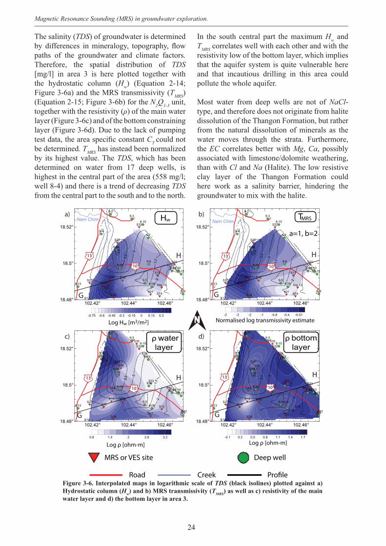
24
Magnetic Resonance Sounding (MRS) in groundwater exploration.
The salinity ( ) of groundwater is determined
paths of the groundwater and climate factors. Therefore, the spatial distribution of [mg/l] in area 3 is here plotted together with the hydrostatic column (Hw) (Equation 2-14; Figure 3-6a) and the MRS transmissivity ( MRS)(Equation 2-15; Figure 3-6b) for the N2Q1-3 unit, together with the resistivity ( ) of the main water layer (Figure 3-6c) and of the bottom constraining layer (Figure 3-6d). Due to the lack of pumping
C could not be determined. MRS has instead been normalized by its highest value. The , which has been determined on water from 17 deep wells, is highest in the central part of the area (558 mg/l; well 8-4) and there is a trend of decreasing from the central part to the south and to the north.
In the south central part the maximum Hw and MRS correlates well with each other and with the
resistivity low of the bottom layer, which implies that the aquifer system is quite vulnerable here and that incautious drilling in this area could pollute the whole aquifer.
Most water from deep wells are not of NaCl-type, and therefore does not originate from halite dissolution of the Thangon Formation, but rather from the natural dissolution of minerals as the water moves through the strata. Furthermore, the EC correlates better with Mg, Ca, possibly associated with limestone/dolomite weathering, than with Cl and Na (Halite). The low resistive clay layer of the Thangon Formation could here work as a salinity barrier, hindering the groundwater to mix with the halite.
102.42° 102.44° 102.46°18.48°
18.5°
18.52°
Site 12
S13
S14
S15
S16
S17
S19S20
S22
S23
S27S28
S32
8-04
8-06
8-08
8-108-12
8-13
8-15
9-29-3
9-4
9-5
9-6
9-7
9-8
9-9
-0.75 -0.6 -0.45 -0.3 -0.15 0 0.15 0.3
13
10
Nam Chim Hw
Log Hw [m3/m2]
G
H
a=1, b=2
Nam ChimTMRS
102.42° 102.44° 102.46°18.48°
18.5°
18.52°
Site 12
S13
S14
S15
S16
S17
S19S20
S22
S23
S27S28
S32
8-04
8-06
8-08
8-108-12
8-13
8-15
9-29-3
9-4
9-5
9-6
9-7
9-8
9-9
-2 -2 -2 -1 -0.8 -0.4 -0.01
Normalised log transmissivity estimate
13
10
G
H
102.42° 102.44° 102.46°18.48°
18.5°
18.52°
S12
S15
S16
S17
S19S20
S22
S27S28
S32
S33
S34
S35
S38
S41
S43
S44
S468-04
8-06
8-08
8-108-12
8-13
8-15
9-29-3
9-4
9-5
9-6
9-7
9-8
9-9
0.8 1.4 2 2.6 3.2
ρ waterlayer
13
10
Log ρ [ohm-m]
G
H
ρ bottomlayer
102.42° 102.44° 102.46°18.48°
18.5°
18.52°
S12
S15
S16
S17
S19S20
S22
S23
S27S28
S32
S33
S34
S35
S38
S39
S41
S43
S44
S468-04
8-06
8-08
8-108-12
8-13
8-15
9-29-3
9-4
9-5
9-6
9-7
9-8
9-9
-0.1 0.2 0.5 0.8 1.1 1.4 1.7
13
10
Log ρ [ohm-m]
G
H
N
MRS or VES site Deep well
Road Creek Profile
a) b)
c) d)
Figure 3-6. Interpolated maps in logarithmic scale of TDSHydrostatic column (Hw) and b) MRS transmissivity (TMRS) as well as c) resistivity of the main water layer and d) the bottom layer in area 3.
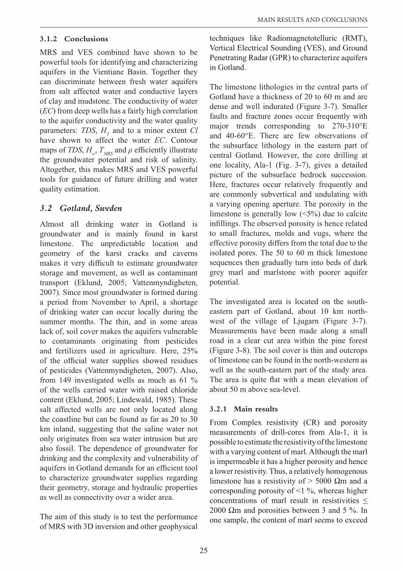
25
MAIN RESULTS AND CONCLUSIONS
3.1.2 Conclusions
MRS and VES combined have shown to be powerful tools for identifying and characterizing aquifers in the Vientiane Basin. Together they can discriminate between fresh water aquifers from salt affected water and conductive layers of clay and mudstone. The conductivity of water (EC) from deep wells has a fairly high correlation to the aquifer conductivity and the water quality parameters: , H and to a minor extent Clhave shown to affect the water EC. Contour maps of , Hw, MRS and the groundwater potential and risk of salinity. Altogether, this makes MRS and VES powerful tools for guidance of future drilling and water quality estimation.
3.2 Gotland, Sweden
Almost all drinking water in Gotland is groundwater and is mainly found in karst limestone. The unpredictable location and geometry of the karst cracks and caverns
storage and movement, as well as contaminant transport (Eklund, 2005; Vattenmyndigheten, 2007). Since most groundwater is formed during a period from November to April, a shortage of drinking water can occur locally during the summer months. The thin, and in some areas lack of, soil cover makes the aquifers vulnerable to contaminants originating from pesticides and fertilizers used in agriculture. Here, 25%
of pesticides (Vattenmyndigheten, 2007). Also, from 149 investigated wells as much as 61 % of the wells carried water with raised chloride content (Eklund, 2005; Lindewald, 1985). These salt affected wells are not only located along the coastline but can be found as far as 20 to 30 km inland, suggesting that the saline water not only originates from sea water intrusion but are also fossil. The dependence of groundwater for drinking and the complexity and vulnerability of
to characterize groundwater supplies regarding their geometry, storage and hydraulic properties as well as connectivity over a wider area.
The aim of this study is to test the performance of MRS with 3D inversion and other geophysical
techniques like Radiomagnetotelluric (RMT), Vertical Electrical Sounding (VES), and Ground Penetrating Radar (GPR) to characterize aquifers in Gotland.
The limestone lithologies in the central parts of Gotland have a thickness of 20 to 60 m and are dense and well indurated (Figure 3-7). Smaller faults and fracture zones occur frequently with
the subsurface lithology in the eastern part of central Gotland. However, the core drilling at one locality, Ala-1 (Fig. 3-7), gives a detailed picture of the subsurface bedrock succession. Here, fractures occur relatively frequently and are commonly subvertical and undulating with a varying opening aperture. The porosity in the limestone is generally low (<5%) due to calcite
to small fractures, molds and vugs, where the effective porosity differs from the total due to the isolated pores. The 50 to 60 m thick limestone sequences then gradually turn into beds of dark grey marl and marlstone with poorer aquifer potential.
The investigated area is located on the south-eastern part of Gotland, about 10 km north-west of the village of Ljugarn (Figure 3-7). Measurements have been made along a small road in a clear cut area within the pine forest (Figure 3-8). The soil cover is thin and outcrops of limestone can be found in the north-western as well as the south-eastern part of the study area.
about 50 m above sea-level.
3.2.1 Main results
From Complex resistivity (CR) and porosity measurements of drill-cores from Ala-1, it is possible to estimate the resistivity of the limestone with a varying content of marl. Although the marl is impermeable it has a higher porosity and hence a lower resistivity. Thus, a relatively homogenous limestone has a resistivity of > 5000 m and a corresponding porosity of <1 %, whereas higher
2000 m and porosities between 3 and 5 %. In one sample, the content of marl seems to exceed
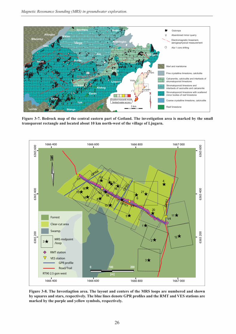
26
Magnetic Resonance Sounding (MRS) in groundwater exploration.
Sjonhem
Viklau
Vänge
Buttle
Ala
EtelhemAlskog
Ardre
Östergarn
Anga
Garda
Lye
Stånga
Lojsa
LindeLevide
AltingboMästerby
Väte
Hejde
Kräklingbo
Ljugarn
5 km
Ala-1
Outcrops
Abandoned minor quarry
Electromagnetic lineament,aerogeophysical measurement
Fine crystalline limestone, calcilutite
Marl and marlstorne
Reef limestone
Coarse crystalline limestone, calcirudite
Stromatoporoid limestone and interbeds of cacirudite and calcarenite
Stromatoporoid limestone with scattered minor bodies of reef limestone
Calcarenite, calcirudite and interbeds ofstromatoporoid limestone
Ala-1 core drilling
Gradient towards morelimited water access
Visby
Fårö
Ljugarn
Investigationarea
1666 6001666 400 1666 800 1667 000
1666 6001666 400 1666 800 1667 000
6365
400
6365
200
20
18 16
97
10
11
GP
R2
GPR1
GPR3
V1
V2
V3
21
1
2
3
4
5
8
12
14
15
13GPR4
V4
619
17
200100
[m]
0
Forrest
Clear-cut area
Swamp
3MRS midpoint/loop
RMT station
VES stationGPR profile
Road/Trail
RT90 2.5 gon west
6365
600
6365
400
6365
200
6365
600
Figure 3-8. The Investiagtion area. The layout and centers of the MRS loops are numbered and shown
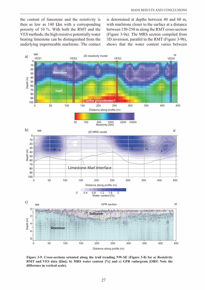
27
MAIN RESULTS AND CONCLUSIONS
the content of limestone and the resistivity is then as low as 140 m with a corresponding porosity of 10 %. With both the RMT and the VES methods, the high resistive potentially water bearing limestone can be distinguished from the underlying impermeable marlstone. The contact
is determined at depths between 40 and 60 m, with marlstone closer to the surface at a distance between 150-250 m along the RMT cross-section (Figure 3-9a). The MRS section compiled from 3D inversion, parallel to the RMT (Figure 3-9b), shows that the water content varies between
c)
Distance along profile (m)
NW SEGPR section
0 50 100 150 200 250 300 350 400 4508
6
4
2
0
limestone
Soil cover
0 50 100 150 200 250 300 350 400 450 100
90 8070
60 50 40 30 20 10
0
Water content [%]0 0.4 0.8 1.2 1.6 2
Distance along profile (m)
NW SE2D MRS modelb)
Limestone-Marl interface
Dep
th (m
)
100 90 80 70 60 50 40 30 20 10
0
2D resistivity model
Distance along profile (m)0 50 100 150 200 250 300 350 400 450
Dep
th (m
)D
epth
(m)
NW SEa)
limestone
marl
saline groundwater?
VES1 VES2 VES3 VES4
Resistivity [Ωm]30 100 300 1000 3200 10000
Figure 3-9. Cross-sections oriented along the trail trending NW-SE (Figure 3-8) for a) Resistivity
difference in vertical scale).
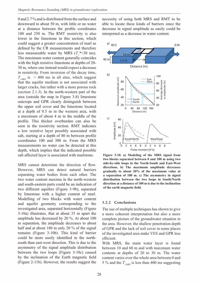
28
Magnetic Resonance Sounding (MRS) in groundwater exploration.
0 and 2.7 % and is distributed from the surface and downward to about 50 m, with little or no water
100 and 250 m. The RMT resistivity is also lower in the limestone in this section, which could suggest a greater concentration of marl as
less measureable water by MRS ( 2*<30 ms). The maximum water content generally coincides with the high resistive limestone at depths of 20-30 m, where one instead would expect a decrease in resistivity. From inversion of the decay time,
1MRS is < 400 ms in all sites, which suggest that the aquifer medium is not associated with larger cracks, but rather with a more porous rock (section 2.1.3). In the north-western part of the area (outside the map in Figure 3-8) limestone outcrops and GPR clearly distinguish between the upper soil cover and the limestone located at a depth of 0.5 m in the western area, with a maximum of about 4 m in the middle of the
seen in the resistivity section. RMT indicates a low resistive layer possibly associated with
coordinates 100 and 300 m. From the MRS measurements no water can be detected at this depth, which implies that the indicated possible salt affected layer is associated with marlstone.
However, MRS can detect natural barriers separating water bodies from each other. Thetwo water content maxima in the north-western and south-eastern parts could be an indication of two different aquifers (Figure 3-9b), separated by limestone with a higher content of marl. Modelling of two blocks with water content and aquifer geometry corresponding to the investigated area, separated horizontally (Figure 3-10a) illustrates, that at about 35 m apart the amplitude has decreased by 20 %. At about 100 m separation, the amplitude decreases to about half and at about 180 m only 20 % of the signal remains (Figure 3-10b). This kind of barrier
south than east-west direction. This is due to the asymmetry of the signal amplitude distribution between the two loops (Figure 3-10c) caused
(Figure 2-11b). However, the results suggest the
necessity of using both MRS and RMT to be able to locate these kinds of barriers since the decrease in signal amplitude as easily could be interpreted as a decrease in water content.
Figure 3-10. a) Modeling of the MRS signal from
side-by-side loops in the North-South and East-West directions. b) The maximum amplitude decreases
a separation of 180 m. c) The asymmetry in signal distribution between the two loops in South/North direction at a distance of 100 m is due to the inclination
0 40 80 120 16020
40
60
80
20
40
60
80
100
Max
imum
am
plitu
de [n
V]
Aver
age
decr
ease
in a
mpl
itude
[%]
Distance [m]
EastWest
SouthNorth
b)
a)
40 m
W/S E/N
10 m
Distance [m]
1.7 %
c)
20 4 6 8 20 4 6 8
South/North West/EastAm
plitu
de [n
V]
Pulse moment [A*s]
0
20
40
60
3.2.2 Conclusions
The use of multiple techniques has shown to give a more coherent interpretation but also a more complete picture of the groundwater situation in the area. However, the shallow penetration depth of GPR and the lack of soil cover in some places of the investigated area make VES and GPR less
With MRS, the main water layer is found between 10 and 60 m and with maximum water contents at depths of 20 to 30 m. The water content varies over the whole area between 0 and 5 % and the 1MRS is less than 400 ms suggesting
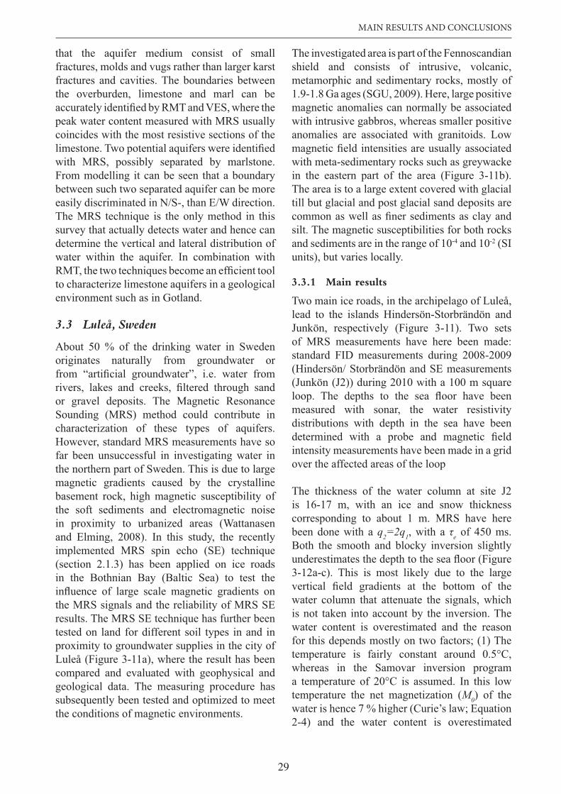
29
MAIN RESULTS AND CONCLUSIONS
that the aquifer medium consist of smallfractures, molds and vugs rather than larger karst fractures and cavities. The boundaries between the overburden, limestone and marl can be
peak water content measured with MRS usually coincides with the most resistive sections of the
with MRS, possibly separated by marlstone. From modelling it can be seen that a boundary between such two separated aquifer can be more easily discriminated in N/S-, than E/W direction. The MRS technique is the only method in this survey that actually detects water and hence can determine the vertical and lateral distribution of water within the aquifer. In combination with
to characterize limestone aquifers in a geological environment such as in Gotland.
3.3 Luleå, Sweden
About 50 % of the drinking water in Sweden originates naturally from groundwater or
or gravel deposits. The Magnetic Resonance Sounding (MRS) method could contribute in characterization of these types of aquifers. However, standard MRS measurements have so far been unsuccessful in investigating water in the northern part of Sweden. This is due to large magnetic gradients caused by the crystalline basement rock, high magnetic susceptibility of the soft sediments and electromagnetic noise in proximity to urbanized areas (Wattanasen and Elming, 2008). In this study, the recently implemented MRS spin echo (SE) technique (section 2.1.3) has been applied on ice roads in the Bothnian Bay (Baltic Sea) to test the
the MRS signals and the reliability of MRS SE results. The MRS SE technique has further been tested on land for different soil types in and in proximity to groundwater supplies in the city of Luleå (Figure 3-11a), where the result has been compared and evaluated with geophysical and geological data. The measuring procedure has subsequently been tested and optimized to meet the conditions of magnetic environments.
The investigated area is part of the Fennoscandian shield and consists of intrusive, volcanic, metamorphic and sedimentary rocks, mostly of 1.9-1.8 Ga ages (SGU, 2009). Here, large positive magnetic anomalies can normally be associated with intrusive gabbros, whereas smaller positive anomalies are associated with granitoids. Low
with meta-sedimentary rocks such as greywacke in the eastern part of the area (Figure 3-11b). The area is to a large extent covered with glacial till but glacial and post glacial sand deposits are
silt. The magnetic susceptibilities for both rocks and sediments are in the range of 10-4 and 10-2 (SI units), but varies locally.
3.3.1 Main results
Two main ice roads, in the archipelago of Luleå, lead to the islands Hindersön-Storbrändön and Junkön, respectively (Figure 3-11). Two sets of MRS measurements have here been made: standard FID measurements during 2008-2009 (Hindersön/ Storbrändön and SE measurements (Junkön (J2)) during 2010 with a 100 m square
measured with sonar, the water resistivity distributions with depth in the sea have been
intensity measurements have been made in a grid over the affected areas of the loop
The thickness of the water column at site J2 is 16-17 m, with an ice and snow thickness corresponding to about 1 m. MRS have here been done with a q2=2q1, with a e of 450 ms. Both the smooth and blocky inversion slightly
3-12a-c). This is most likely due to the large
water column that attenuate the signals, which is not taken into account by the inversion. The water content is overestimated and the reason for this depends mostly on two factors; (1) The
whereas in the Samovar inversion program
temperature the net magnetization (M0) of the water is hence 7 % higher (Curie’s law; Equation 2-4) and the water content is overestimated
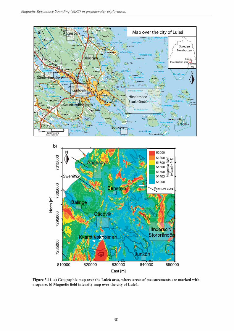
30
Magnetic Resonance Sounding (MRS) in groundwater exploration.
8ki lometers
Scale: 1:256 400
0 4
Map over the city of LuleåÄngesbyn
Sandnäsudden
Bensbyn
Gäddvik
Hindersön/Storbrändön
Junkön
Kvarnträskholmen
810000 820000 830000 840000 850000East [m]
7285
000
7295
000
7305
000
7315
000
Nor
th [m
]
Ängesbyn
Gäddvik
Hindersön/Storbrändön
Sweref99
N
51000
5140051500516005170051800
52000
Mag
netic
fiel
d In
tens
ity [n
T]
Luleå
BothniaBay
SwedenNorrbotten
Investigation area
a)
b)
N
Junkön
Fracture zone
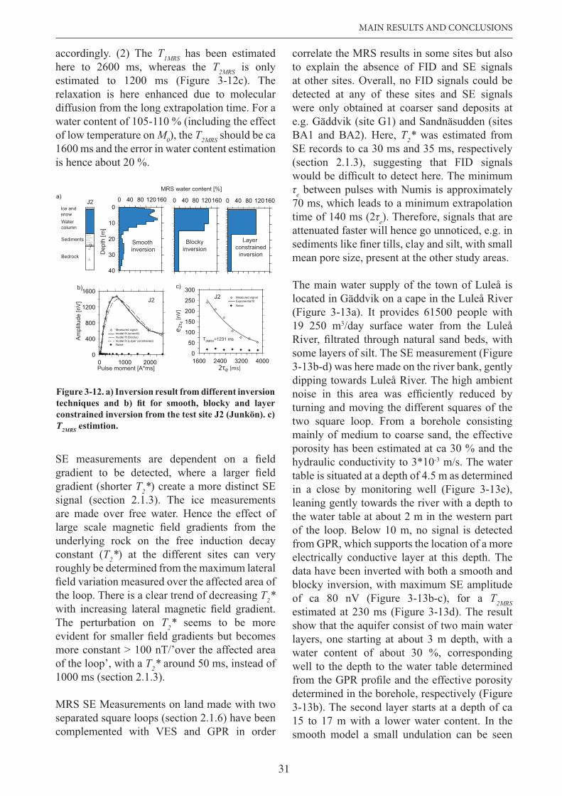
31
MAIN RESULTS AND CONCLUSIONS
accordingly. (2) The 1MRS has been estimated here to 2600 ms, whereas the 2MRS is only estimated to 1200 ms (Figure 3-12c). The relaxation is here enhanced due to molecular diffusion from the long extrapolation time. For a water content of 105-110 % (including the effect of low temperature on M0), the 2MRS should be ca 1600 ms and the error in water content estimation is hence about 20 %.
correlate the MRS results in some sites but also to explain the absence of FID and SE signals at other sites. Overall, no FID signals could be detected at any of these sites and SE signals were only obtained at coarser sand deposits at e.g. Gäddvik (site G1) and Sandnäsudden (sites BA1 and BA2). Here, 2* was estimated from SE records to ca 30 ms and 35 ms, respectively (section 2.1.3), suggesting that FID signals
e between pulses with Numis is approximately 70 ms, which leads to a minimum extrapolation time of 140 ms (2 e). Therefore, signals that are attenuated faster will hence go unnoticed, e.g. in
mean pore size, present at the other study areas.
The main water supply of the town of Luleå is located in Gäddvik on a cape in the Luleå River (Figure 3-13a). It provides 61500 people with 19 250 m3/day surface water from the Luleå
some layers of silt. The SE measurement (Figure 3-13b-d) was here made on the river bank, gently dipping towards Luleå River. The high ambient
turning and moving the different squares of the two square loop. From a borehole consisting mainly of medium to coarse sand, the effective porosity has been estimated at ca 30 % and the hydraulic conductivity to 3*10-3 m/s. The water table is situated at a depth of 4.5 m as determined in a close by monitoring well (Figure 3-13e), leaning gently towards the river with a depth to the water table at about 2 m in the western part of the loop. Below 10 m, no signal is detected from GPR, which supports the location of a more electrically conductive layer at this depth. The data have been inverted with both a smooth and blocky inversion, with maximum SE amplitude of ca 80 nV (Figure 3-13b-c), for a 2MRSestimated at 230 ms (Figure 3-13d). The result show that the aquifer consist of two main water layers, one starting at about 3 m depth, with a water content of about 30 %, corresponding well to the depth to the water table determined
determined in the borehole, respectively (Figure 3-13b). The second layer starts at a depth of ca 15 to 17 m with a lower water content. In the smooth model a small undulation can be seen
0 40 80 120160
40
30
20
10
00 40 80 120160
MRS water content [%]
Dep
th [m
]
0 40 80 120160
Watercolumn
Sediments
Ice and snow
Bedrock
?
a)
1600 2400 3200 40000
50
100
150
200
250
300
2τe [ms]
e 2τ e
[nV]
Measured signalExponential fitNoise
J2
T2MRS=1231 ms
c)
Smoothinversion
Blockyinversion
Layerconstrained
inversion
0 1000 20000
400
800
1200
1600b)
Measured signalmodel fit (smooth)model fit (blocky)model fit (Layer constrained)Noise
J2
Pulse moment [A*ms]
Am
plitu
de [n
V]
J2
Figure 3-12. a) Inversion result from different inversion
T2MRS estimtion.
gradient (shorter 2*) create a more distinct SE signal (section 2.1.3). The ice measurements are made over free water. Hence the effect of
underlying rock on the free induction decay constant ( 2*) at the different sites can very roughly be determined from the maximum lateral
the loop. There is a clear trend of decreasing 2*
The perturbation on 2* seems to be more
more constant > 100 nT/’over the affected area of the loop’, with a 2* around 50 ms, instead of 1000 ms (section 2.1.3).
MRS SE Measurements on land made with two separated square loops (section 2.1.6) have been complemented with VES and GPR in order
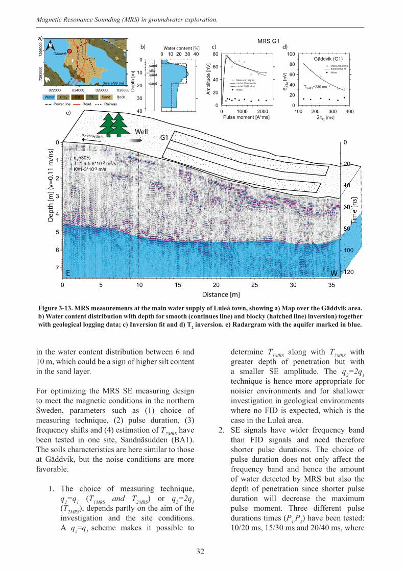
32
Magnetic Resonance Sounding (MRS) in groundwater exploration.
in the water content distribution between 6 and10 m, which could be a sign of higher silt content in the sand layer.
For optimizing the MRS SE measuring design to meet the magnetic conditions in the northern Sweden, parameters such as (1) choice of measuring technique, (2) pulse duration, (3) frequency shifts and (4) estimation of 2MRS have been tested in one site, Sandnäsudden (BA1). The soils characteristics are here similar to those at Gäddvik, but the noise conditions are more favorable.
1. The choice of measuring technique, q2=q1 ( 1MRS 2MRS) or q2=2q1( 2MRS), depends partly on the aim of the investigation and the site conditions. A q2=q1 scheme makes it possible to
determine 1MRS along with 2MRS with greater depth of penetration but with a smaller SE amplitude. The q2=2q1technique is hence more appropriate for noisier environments and for shallower investigation in geological environments where no FID is expected, which is the case in the Luleå area.
2. SE signals have wider frequency band than FID signals and need therefore shorter pulse durations. The choice of pulse duration does not only affect the frequency band and hence the amount of water detected by MRS but also the depth of penetration since shorter pulse duration will decrease the maximum pulse moment. Three different pulse durations times (P P2) have been tested: 10/20 ms, 15/30 ms and 20/40 ms, where
2
7
6
5
4
3
2
1
0
0 5 10 15 20 25 30 35
20
20
0G1
Distance [m]
Dep
th [m
] (v=
0.11
m/n
s)
Well
WE
MRS G1
100 200 300 4000
20
40
60
80
100
2τe [ms]
e 2τ e
[nV]
Gäddvik (G1)Measured signalExponential fitNoise
T2MRS=230 ms
a)b) d)
0 1000 20000
20
40
60
80
Measured signalmodel fit (smooth)model fit (blocky)Noise
Pulse moment [A*ms]
Am
plitu
de [n
V]
40
30
20
10
0sandsiltysand
sand
Dep
th [m
]
e)
c)0 10 20 30 40
Water content [%]
Borehole 30 m
822000 824000 826000 828000
N
Gäddvik7295
000
7293
000
Water SiltClay Till Sand
Road RailwayPower line
Sweref99 [m]
Rock
ne≈30%T=1.6-5.8*10-2 m2/sK=1-3*10-3 m/s
33
SUMMARY
it can be seen that the pulse moment and
the different pulse durations. However a P1 15 ms seems to be a best compromise for this type of deposit, considering depth of penetration and measurable water content.
3. Due to the magnetic gradients present in SE measurements, frequency shifts occur in the data. At site BA1, ±10 Hz frequency shift corresponds to a decrease in maximum SE amplitude of more than 50 %, whereas ±5 Hz correspond to a decrease of 25 %. From inversion it can be seen that frequency shifts smaller than < 5 Hz have smaller impact on the
water content and thickness. 4. By measuring the 2MRS for different
pulse moments with coherent values, the estimation of 2MRS seems to give reliable results.
3.3.2 Conclusions
MRS SE measurements have shown to give reliable results from measurements on ice over open water, although, 2MRS and hence the water content estimation are clearly affected by diffusion due to the long extrapolation time. From
is noticed that gradients > 100 nT/’affected area of the loop’ can diminish the 2* from 1000 ms to < 50 ms. On land, the two separated square
by careful adjustment of the loop layout. MRS SE showed to be suitable for locating aquifers
to the instrument limitation of minimum delay time, leaving signals <140 ms unrecorded. MRS SE result from the site of the Luleå town water supply shows a good agreement with the estimated effective porosity and aquifer geometry from a nearby borehole and it has been showed that a standard SE measuring procedure with pulse durations of 15/30 ms works best in this type of geology.
4 SUMMARY
Groundwater from a global perspective provides about 50 % of the potable-, 40 % of the industrial- and 20 % of the irrigation water. For drinking water, deep groundwater has many advantages compared to surface water and shallow groundwater, since it demands little or no treatment and the access is secured against temporary droughts. However, drilling wells is
knowing the groundwater potential, therefore development of techniques for exploration are of high priority. In this thesis, results fromthree different types of geological environmentsusing the Magnetic Resonance Sounding (MRS) technique have been presented. MRS is based on the principle of nuclear magnetic resonance, and it is in contrast to other geophysical techniques directly sensitive to water.
The sedimentary basin of Vientiane, Laos, with naturally occurring salt in the bedrock at depths as shallow as 50 m, inevitably affects drinking and irrigation water from deep wells. Here MRS and Vertical Electrical Sounding (VES) together with water quality samples from shallow and deep wells have been used to characterize the different geological units in the basin as well as distinguish freshwater aquifers from salt affected water, conductive clay and mudstone with good results. The electric conductivity of the aquifers has then been compared with the conductivity of water from wells, with a poor correlation for shallow wells but a fairly good linear correlation for deep wells (R2=0.69). This is probably due to the higher water content and salinity of the deeper water contributing more to the aquifer conductivity. The water quality parameters most affected by the electric conductivity of water are total dissolved solids ( ), hardness and to a minor extent chloride. Contour maps of ,MRS transmissivity, MRS hydrostatic column together with VES resistivity of the aquifer
groundwater potential and risk of salinisation of the investigated area. Altogether, this makes MRS and VES a powerful tool for guidance of future drilling and water quality estimation.
34
Magnetic Resonance Sounding (MRS) in groundwater exploration.
In karst limestone with underlying marl, on the island of Gotland, Sweden, saltwater intrusion, both recent and relic together with pollution from pesticides and fertilizers, are major threats to an already exhausted drinking water resource. Here, the performance of MRS together with VES, Radiomagnetotelluric (RMT), and Ground Penetrating Radar (GPR) was tested
the central eastern part of the island. The use of multiple techniques has shown to give a more coherent interpretation but also a more complete picture of the groundwater distribution in the area. However, the shallow penetration depth of GPR and the lack of soil cover in some places of the investigated area make VES and GPR less
the potentially water bearing limestone and
by RMT and VES. The peak water content measured with MRS usually coincides with the most resistive sections of the limestone. There are
by a more marl rich limestone. Modelling of two water saturated blocks separated from each other shows that such barrier would be more easily detected in N/S direction than E/W due to asymmetry of the signal distribution caused by
information is important when evaluating the risk of dissemination of contaminations from e.g. salt or pesticides. Altogether, MRS is the only method in this survey that actually detects water and in combination with RMT, they become
in a geological environment such as in Gotland.
In Norrbotten, Sweden, the magnetic environment has made it impossible to use standard MRS to characterize the many natural sand or gravel deposits, which constitutes 50 % of the country’s drinking water resources. Instead, the recent Spin-Echo (SE) technique has been implemented and tested with measurements from ice, in the Bothnian Bay and on land, in and around the city of Luleå. Measurements from the ice showed reliable results in terms of geometry of the water column. However the water content was overestimated. This was due to the enhanced diffusion relaxation caused by the long extrapolation time in the SE-measurement. It
was also shown that lateral magnetic gradients of 100 nT/’affected area of the loop’ can diminish the 2* from 1000 ms to < 50 ms. On land, the
by careful adjustment of the loop layout. MRS SE showed to be suitable for locating aquifers
to instrument limitation of a minimum delay of 70 ms, which means that signals relaxed sooner than 140 ms will not be recorded with current Numis technology. MRS SE result from the site of the Luleå town water supply shows a good agreement with estimated effective porosity and the geometry of the aquifer from a near by borehole and it has been showed that a standard SE measuring procedure with pulse durations of 15/30 ms works best in this type of geology. Small frequency shifts have little effect on the inversion result and 2MRS measurements for different pulse moments give coherent and thus reliable results.
The close relation with hydrogeological parameters and the robust theoretical foundation of the MRS method makes it a very appealing technique to use in groundwater exploration. The often complex acquisition procedure and limitations concerning noise, electrically conductive mediums and magnetic inhomogeneities can be overcome. In the studies
in the geological environments tested and morover MRS has decreased the ambiguity in the geological/hydrological interpretation.
35
REFERENCES
5 REFERENCES
Allen, D. et al., 1997. How to use borehole
summer, pp. 34-57.Archie, G.E., 1942. The electrical resistivity log
as an aid in determining some reservoir characteristics. Metallurgical and Petroleum Engineers 146: 54-62.
Bastani, M., 2001. EnviroMT- A New Controlled Source/Radio Magnetotelluric System Ph.D. Acta Universitatis Upsaliensis, Uppsala Dissertations from the Faculty of Science and Technology 32.
Bates, B.C.E., Kundzewicz, Z.W., Wu, S., Palutikof, J.P., 2008. Climate Change and Water. Technical Paper of the Intergovernmental Panel on Climate Change, IPCC Secretariat, Geneva, 210 pp.
measure a magnetic resonance sounding. Boletín geológico y minero, 118(3): 459-472.
Boucher, M., Favreau, G., Vouillamoz, J.M., Nazoumou, Y., Legchenko, A.,
transmissivity with magnetic resonance
aquifer (Niger). Hydrogeology Journal, 17(7): 1805-1815.
Braun, M., Hertrich, M., Yaramanci, U., 2005. Study on complex inversion of magnetic resonance sounding signals. NEAR SURF GEOPHYS, 3(3): 155-163.
Clesceri, L.S.E., Greenberg, A.E.E., Eaton, A.D.E., 1998. Standard Methods for the Examination of Water and Wastewater. Americal Public Health Association (Washington), American Water Works Association (Denver), and Water Environment Federation (Alexandria, VA), 1220 pp.
Darcy, H., 1856. Les Fontaines Publiques de la Ville de Dijon, Dalmont, Paris.
Dlugosch, R., Mueller-Petke, M., Günther, T., Costabel, S., Yaramanci, U., 2011. Assessment of the potential of a new generation of surface nuclear magnetic resonance instruments. NEAR SURF GEOPHYS, 9: 89-102.
Dongen, P.v., Woodhouse, M., 1994. Findining Groundwater-A Project Manager’s Guide to Techniques and How to Use Them, UNDP-World Bank/Water and Sanitation Program.
Dunn, K.J., Bergman, D.J., Latorraca, G.A., 2002. Nuclear magnetic resonance, petrophysical and logging applications. Handbook of geophysical exploration. Seismic exploration, vol. 32, 282 pp.
Eklund, F., 2005. Förändringar i grundvattenkvaliteten i 19 vattentäkter på Gotland under åren 1989-2004. Länsstyrelsen i Gotlands län, Visby, 133 pp.
El Tabakh, M., Utha-Aroon, C., Schreiber, B.C., 1999. Sedimentology of the Cretaceous Maha Sarakham evaporites in the Khorat Plateau of northeastern Thailand. Sedimentary Geology, 123(1-2): 31-62.
Girard, J.F., Boucher, M., Legchenko, A., Baltassat, J.M., 2007. 2D magnetic resonance tomography applied to karstic conduit imaging. J APPL GEOPHYS, 63(3-4): 103-116.
Grunewald, E., Knight, R., 2011. The effect of pore size and magnetic susceptibility on the surface NMR relaxation parameter T2*. NEAR SURF GEOPHYS, 9: 169-178.
Guillen, A., Legchenko, A., 2002a. Application of linear programming techniques to the inversion of proton magnetic resonance measurements for water prospecting from the surface. J APPL GEOPHYS, 50(1-2): 149-162.
Guillen, A., Legchenko, A., 2002b. Inversion of surface nuclear magnetic resonance data by an adapted Monte Carlo method applied to water resource characterization. J APPL GEOPHYS, 50(1-2): 193-205.
Hahn, E.L., 1950. Spin Echoes. Physical review, 80(4): 580-594.
Hertrich, M., 2008. Imaging of groundwater with nuclear magnetic resonance. Progress in Nuclear Magnetic Resonance Spectroscopy, 53(4): 227-248.
Hertrich, M., Yaramanci, U., 2002. Joint inversion of Surface Nuclear Magnetic Resonance and Vertical Electrical Sounding. J APPL GEOPHYS, 50(1-2): 179-191.
36
Magnetic Resonance Sounding (MRS) in groundwater exploration.
Iris-Instruments, 2005. NUMIS - MRS (Magnetic Resonance Sounding) SYSTEM - User’s manual (electronic resource). http://www.iris-instruments.com/.
JICA, 1993. Design Study Report on the Project for Groundwater Development in Vientiane Province in Lao People’s Democratic Republic. Japan International Cooperation Agency (JICA), 94 pp.
JICA, 1994. Drilling logs from the “Groundwater Development in the Vientiane Province Project”. Japan International Cooperation
Phon Hong, Vientiane Province, Laos., pp. 718.
JICA, 2000. The study on rural water supply and sanitation improvement in the northwest region in the Lao People´s Democratic Republic, Progress report 2,. Japan International Cooperation Agency (JICA), 14 pp.
Kalscheuer, T., Pedersen, L.B., Siripunvaraporn, W., 2008. Radiomagnetotelluric two-dimensional forward and inverse modelling accounting for displacement currents. Geophys J Int, 175(2): 486-514.
Keating, K., Knight, R., 2007. A laboratory study to determine the effect of iron oxides on proton NMR measurements. GEOPHYSICS, 72(1): E27-E32.
Keating, K., Knight, R., 2008. A laboratory study of the effect of magnetite on NMR relaxation rates. J APPL GEOPHYS, 66(3-4): 188-196.
Kenyon, W.E., 1997. Petrophysical principles of applications of NMR logging. The log analyst, March-April: 21-43.
Kirsch, R. (Ed.), 2006. Groundwater Geophysics: a Tool for Hydrogeology. Springer - Verlag, Berlin Heidelberg, 493 pp.
Knödel, K., Lange, G., Voigt, H.-J. (Eds.), 2008. Environmental Geology : Handbook of Field Methods and Case Studies. Springer-Verlag, Berlin, Heidelberg, 1357 pp.
Krawczyk, W.E., Ford, D.C., 2006. Correlating
in limestone and dolomite karst waters. Earth Surface Processes and Landforms, 31(2): 221-234.
Krawczyk, W.E., Ford, D.C., 2007. Correlating
in gypsum karst waters. Earth Surface Processes and Landforms, 32(4): 612-620.
Legchenko, A., 2007. MRS measurements and inversion in presence of EM noise. Boletin Geológico y Minero, 118 (3): 489-508.
Legchenko, A., Baltassat, J.M., Beauce, A., Bernard, J., 2002. Nuclear magnetic resonance as a geophysical tool for hydrogeologists. J APPL GEOPHYS, 50(1-2): 21-46.
Legchenko, A. et al., 2004. Magnetic resonance sounding applied to aquifer characterization. GROUND WATER, 42(3): 363-373.
Legchenko, A. et al., 2011. Three-dimensional magnetic resonance imaging for groundwater. New Journal of Physics, 13: 1-18.
Legchenko, A. et al., 2008. Interpretation of magnetic resonance soundings in rocks with high electrical conductivity. J APPL GEOPHYS, 66(3-4): 118-127.
Legchenko, A., Valla, P., 2002. A review of the basic principles for proton magnetic resonance sounding measurements. J APPL GEOPHYS, 50(1-2): 3-19.
Legchenko, A., Valla, P., 2003. Removal of power-line harmonics from proton magnetic resonance measurements. J APPL GEOPHYS, 53(2-3): 103-120.
Legchenko, A., Vouillamoz, J.-M., Roy, J., 2010. Application of the magnetic resonance sounding method to the investigation of aquifers in the presence of magnetic materials. GEOPHYSICS, 75(6): L91-L100.
Legchenko, A.V., Shushakov, O.A., 1998. Inversion of surface NMR data. GEOPHYSICS, 63(1): 75-84.
Lindewald, H., 1985. Salt grundvatten i Sverige, rapporter och meddelanden. 39, Sveriges geologiska undersökning, Uppsala.
37
REFERENCES
Long, N.X., Lam, N.X., Canh, N.D., 1986. Report on Geological data for Potassium and Manganese in Thangon Region, Dong Bang, Vientiane, Department of Geology and Mining, Vientiane, Laos, Vientiane.
López-Geta, J.A., Fornés, J.M., Ramos, G., Villarroya, F., 2001. Groundwater - A natural underground resource. INSTITUTO GEOLÓGICO Y MINERO DE ESPAÑA, pp. 107.
Lubczynski, M., Roy, J., 2003. Hydrogeological interpretation and potential of the new magnetic resonance sounding (MRS) method. J HYDROL, 283(1-4): 19-40.
Lubczynski, M., Roy, J., 2005. MRS contribution to hydrogeological system parametrization. NEAR SURF GEOPHYS, 3(3): 131-139.
Lubczynski, M., Roy, J., 2007. Use of MRS for hydrogeological system parmeterization and modeling. Boletin Geológico y Minero, 118 (3): 509-530.
Medlicott, K., 2001. Water, sanitation and environmental health in rural Laos PDR. KAP Study for UNICEF, WES Section, 20 pp.
Mohnke, O., Yaramanci, U., 2002. Smooth and block inversion of surface NMR amplitudes and decay times using simulated annealing. J APPL GEOPHYS, 50(1-2): 163-177.
Müller-Petke, M., 2009. Extended use of Magnetic Resonance Sounding (MRS) datasets - QT inversion and resolution studies. PhD Thesis, der Technischen Universität Berlin, Berlin, 125 pp.
Palacky, G.J., 1987. Clay mapping using electromagnetic methods European association of exploration geophysicists. Meeting. 48 (06/1986) First break, pp. 295-306.
Parasnis, D.S., 1997. Principles of applied geophysics. Chapman & Hall, 429 pp.
Pelton, W.H., Ward, S.H., Hallof, P.G., Sill, W.R., Nelson, P.H., 1978. Mineral Discrimination and Removal of Inductive Coupling with Multifrequency-Ip. GEOPHYSICS, 43(3): 588-609.
Plata, J., 1999. Técnicas convencionales de
Hidrogeología. Actualidad de las técnicas Geofísicas aplicadas en Hidrogeología. Granada. 21-32 (in Spanish).
Plata, J.L., Rubio, F.M., 2007. Basic theory of the Magnetic Resonance Sounding Method. Boletin Geológico y Minero, 118 (3): 441-458.
Plata, J.L., Rubio, F.M., 2008. The use of MRS in the determination of hydraulic transmissivity: The case of alluvial aquifers. J APPL GEOPHYS, 66(3-4): 128-139.
Reynolds, T., Richards, P., 1996. Unit operations and processes in Environmental Engineering. PWS Publishing Company, Boston, USA, 798 pp.
Roy, J., Rouleau, A., Chouteau, M., Bureau, M., 2008. Widespread occurrence of aquifers currently undetectable with the MRS technique in the Grenville geological province, Canada. J APPL GEOPHYS, 66(3-4): 82-93.
Semenov, A.G., 1987. NMR Hydroscope for water prospecting, Proceedings of the seminar on Geotomography. Indian Geophysical Union, Hyderabad, pp. 66-67.
Sen, P.N., 1988. Electrical conduction in clay bearing sandstones at low and high salinities. J Appl Phys, 63(10): 4832.
and engineers Lewis Publishers, Boca Raton, 444 pp.
SEPA, 2000. Environmental Quality Criteria - Groundwater. REPORT 5051. Swedish Environmental Protection Agency (SEPA), Kalmar, 142 pp.
SGU, 2009. Map services. Geological Survey of Sweden. http://www.sgu.se/sgu/eng/produkter-tjanster/tjanster/kart-tjanst_start_e.html, Uppsala.
Shiklomanov, I.A., UNESCO, 1999. Trends and forecasts in water use [electronic resource]. http://webworld.unesco.org/water/ihp/db/shiklomanov/part’3/HTML/Tb_18.html (Accessed July 05, 2011). UNEP/GRID-Arendal.
38
Magnetic Resonance Sounding (MRS) in groundwater exploration.
Shirov, M., Legchenko, A., Creer, G., 1991. A new direct non-invasive groundwater detection technology for Australia. Exploration Geophysics 22: 333-338.
Shushakov, O.A., 1996. Groundwater NMR in conductive water. GEOPHYSICS, 61(4): 998-1006.
Singh, V.P., Hubbard, S.S., Rubin, Y. (Eds.), 2005. Hydrogeophysics [electronic resource]. Springer, Dordrecht, 523 pp.
Siripunvaraporn, W., Egbert, G., 2000. An
method for 2-D magnetotelluric data. GEOPHYSICS, 65(3): 791-803.
Triumf, C.-A., Thunehed, H., Antal, I., 2000. Bestämning av elektriska egenskaper hos vulkaniter från Skellefte- och Arvidsjaurgrupperna. Sveriges geologiska undersökning 2000:8: 30 pp.
Trushkin, D.V., Shushakov, O.A., Legchenko, A.V., 1994. The Potential of a Noise-Reducing Antenna for Surface NMR Groundwater Surveys in the Earths Magnetic-Field. Geophysical Prospecting, 42(8): 855-862.
UNEP/GRID-Arendal, 2002a. Freshwater availability: groundwater and river
Graphics Library. http://maps.grida.no/go/graphic/freshwater-availability-
date: 5 July 2011].UNEP/GRID-Arendal, 2002b. Groundwater:
aquifers, wells and circulation. UNEP/GRID-Arendal Maps and Graphics Library, http://maps.grida.no/go/graphic/groundwater_aquifers_wells_and_circulation (Accessed 5 July 2011)
UNEP/GRID-Arendal, 2002c. Trends and forecasts in water use, by sector. UNEP/GRID-Arendal Maps and Graphics Library, http://maps.grida.no/go/graphic/trends-and-forecasts-in-water-use-by-sector (Accessed 5 July 2011)
UNESCO, 2003. Water for People Water for Life-Executive Summary-The United Nations World Water Development Report [electronic resource], Paris, 36 pp.
US Salinity Laboratory Staff, 1954. Diagnosis and Improvement of Saline and Alkali Soils. USDA Agric. Handb. 60. U.S. Gov.
Walsh, D.O., Grunewald, E., Turner, P., Hinnell, A., Ferre, P., 2011. Practical limitations and applications of short dead time surface NMR. NEAR SURF GEOPHYS, 9: 103-111.
Wattanasen, K., Elming, S.A., 2008. Direct and indirect methods for groundwater investigations: A case-study of MRS and VES in the southern part of Sweden. J APPL GEOPHYS, 66(3-4): 104-117.
Vattenmyndigheten, 2007. Miljöövervakning av vatten - tillstånd hos inlands-, kust- och grundvatten i Södra Östersjöns vattendistrikt, Kalmar, 186 pp.
Waxman, M.H., Smits, L.J.H., 1968. Electrical conductivities in oil-bearing shale sands. Soc. Petrol. Eng. J., Trans. AIME, vol 243: 107-122.
Weichman, P.B., Lun, D.R., Ritzwoller, M.H., Lavely, E.M., 2002. Study of surface nuclear magnetic resonance inverse problems. J APPL GEOPHYS, 50(1-2): 129-147.
WHO, 1996. Guidelines for drinking-water quality, third edition, incorporating
Recommendations, Geneva, 210-220 pp.WHO, 2004. Water, Sanitation and Hygiene
- Links to Health - FACTS AND FIGURES. http://www.who.int/water_
Vouillamoz, J.M., Baltassat, J.M., Girard, J.F., Plata, J., Legchenko, A., 2007a. Hydrogeological experience in the use of MRS. Boletin Geológico y Minero, 118 (3): 531-550.
Vouillamoz, J.M., Chatenoux, B., Mathieu, F., Baltassat, J.M., Legchenko, A., 2007b.
characterize coastal aquifer in Myanmar. J APPL GEOPHYS, 61(2): 142-154.
Vouillamoz, J.M., Descloitres, M., Toe, G., Legchenko, A., 2005. Characterization of crystalline basement aquifers with MRS: comparison with boreholes and pumping tests data in Burkina Faso. NEAR SURF GEOPHYS, 3(3): 205-213.
39
REFERENCES
Vouillamoz, J.M., Legchenko, A., Nandagiri, L., 2011. Characterizing aquifers when using magnetic resonance sounding in a
SURF GEOPHYS, 9: 135-144.Yaramanci, U., 2009. Surface nuclear
magnetic resonance-A unique tool for hydrogeophysics. The leading edge, 28(10): 1240.
Yaramanci, U., Hertrich, I., 2007. Inversion of Magnetic Resoance Sounding data. Boletin Geológico y Minero, 118 (3): 473-488.
Yaramanci, U., Lange, G., Hertrich, M., 2002. Aquifer characterisation using Surface NMR jointly with other geophysical techniques at the Nauen/Berlin test site. J APPL GEOPHYS, 50(1-2): 47-65.

40
Magnetic Resonance Sounding (MRS) in groundwater exploration.
Paper I
Characterization of aquifers in the Vientiane Basin, Laos, using Magnetic Resonance Sounding and Vertical Electrical Sounding.
Perttu, N., Wattanasen, K., Phommasone, S-Å., Elming (2011) Journal of Applied Geophysics, 73: 207-220.

Characterization of aquifers in the Vientiane Basin, Laos, using Magnetic ResonanceSounding and Vertical Electrical Sounding
Nils Perttu a,⁎, Kamhaeng Wattanasen a,b, Khamphouth Phommasone c, Sten-Åke Elming a
a Division of Geosciences, Luleå University of Technology, SE-971 87 Luleå, Swedenb Department of Physics, Faculty of Science, Prince of Songkla University, HatYai, 90112 Thailandc Department of Physics, National University of Laos, P.O. Box 7322, DongDok Campus Vientiane, Lao Democratic People's Republic
a b s t r a c ta r t i c l e i n f o
Article history:Received 2 June 2009Accepted 4 January 2011Available online 15 January 2011
Keywords:GeophysicsGroundwaterAquifer characterizationKhorat PlateauMagnetic Resonance SoundingVertical Electrical Sounding
The aim of this study is to define and characterize water bearing geological formation and to test thepossibility of using geophysical techniques to determine the hydrogeological parameters in three areas in theVientiane basin, Laos. The investigated areas are part of the Khorat Plateau where halite is naturally occurringat depths as shallow as 50 m in the Thangon Formation. Magnetic Resonance Sounding (MRS) has been usedin combination with Vertical Electrical Sounding (VES) in different geological environments. In total, 46 siteshave been investigated and the MRS and VES recognized the stratigraphic unit N2Q1–3, consisting of alluvialunconsolidated sediments, as the main water bearing unit. The aquifer thickness varies usually between 10and 40 m and the depth to the main aquifer range from 5 to 15 m. The free water content is here up to 30%,and the decay times vary between 100 and 400 ms, suggesting a mean pore size equivalent to fine sand togravel. The resistivity is highly variable, but usually around 10–1500 Ω-m, except for some sites in areas 1and 2, where the aquifer is of low resistivity, probably related to salt water. Hydraulic and storage-relatedparameters such as transmissivity, hydraulic column, have been estimated from the MRS. The MRS togetherwith VES has been shown to be a useful and important tool for identifying and distinguishing freshwater frompossible salt-affected water as well as the salt-related clay layer of the Thangon Formation. This clay layer ischaracterized by very low free water content and a resistivity lower than 5 Ω-m and can be found in all 3 areasat depths from 15 to 50 m.
© 2011 Elsevier B.V. All rights reserved.
1. Introduction
Lao People's Democratic Republic (Laos) is located in the middle ofsouth-east Asia bordering on Thailand, China, Burma (Myanmar),Vietnam and Cambodia (Fig. 1a).
Laos possesses great water resources as it has been estimated that35% of all water in the Mekong River originates from watersheds inLaos, where 80% of the precipitation falls in the rainy season. The twomost important socio-economic sectors to take advantage of thisnatural resource are irrigation and hydropower (STEA, 2001). Theannual renewable fresh water supply per capita amounts to54,000 m3/person, compared to the current demand of 228 m3/person. This makes Laos the richest country in Asia for renewablefreshwater per capita. Still, only 60% of the urban and 51% of the ruralpopulation had direct access to a water supply in 1998 (STEA, 2001).The Vientiane Basin is located in the central part of Laos on the outeredge of the Khorat Plateau. In the basin, natural salt layers are found inthe Thangon Formation. This affects the groundwater quality in some
deep wells (JICA, 2000). Salinity problems are common in central Laosand central-eastern Thailand and have been studied by among othersSrisuk et al. (1999), Wannakomol (2005), and Williamson et al.(1989).
Most Lao people live in the countryside and are heavily dependenton dug wells as their main water source, but also deep wells, riverwater and rainwater are used (Medlicott, 2001). Dugwells usually dryout during the dry period and in addition, water-borne diseasescaused by the infiltration of domestic waste and excreta from farmanimals, has led to a highmorbidity rate (JICA, 1993;Medlicott, 2001).Deep groundwater has many advantages compared to surface waterand shallow groundwater, since it demands little or no treatment andaccess is secured against temporary droughts. However, for explora-tion the small topography difference in the Vientiane Basin makes itdifficult to evaluate the groundwater potential from the visiblephysical environment. Deep wells are expensive and unprofitable ifdrilling is made without knowing the groundwater potential and thelocation of salt-affected groundwater. Therefore, basic informationthat can guide drilling is essential.
One aim of this study is to investigate the efficiency of usingMagnetic Resonance Sounding (MRS) to define and characterize waterbearing geological formations according to their hydraulic and storage
Journal of Applied Geophysics 73 (2011) 207–220
⁎ Corresponding author. Tel.: +46 920 491884; fax: +46 920 491199.E-mail address: [email protected] (N. Perttu).
0926-9851/$ – see front matter © 2011 Elsevier B.V. All rights reserved.doi:10.1016/j.jappgeo.2011.01.003
Contents lists available at ScienceDirect
Journal of Applied Geophysics
j ourna l homepage: www.e lsev ie r.com/ locate / jappgeo
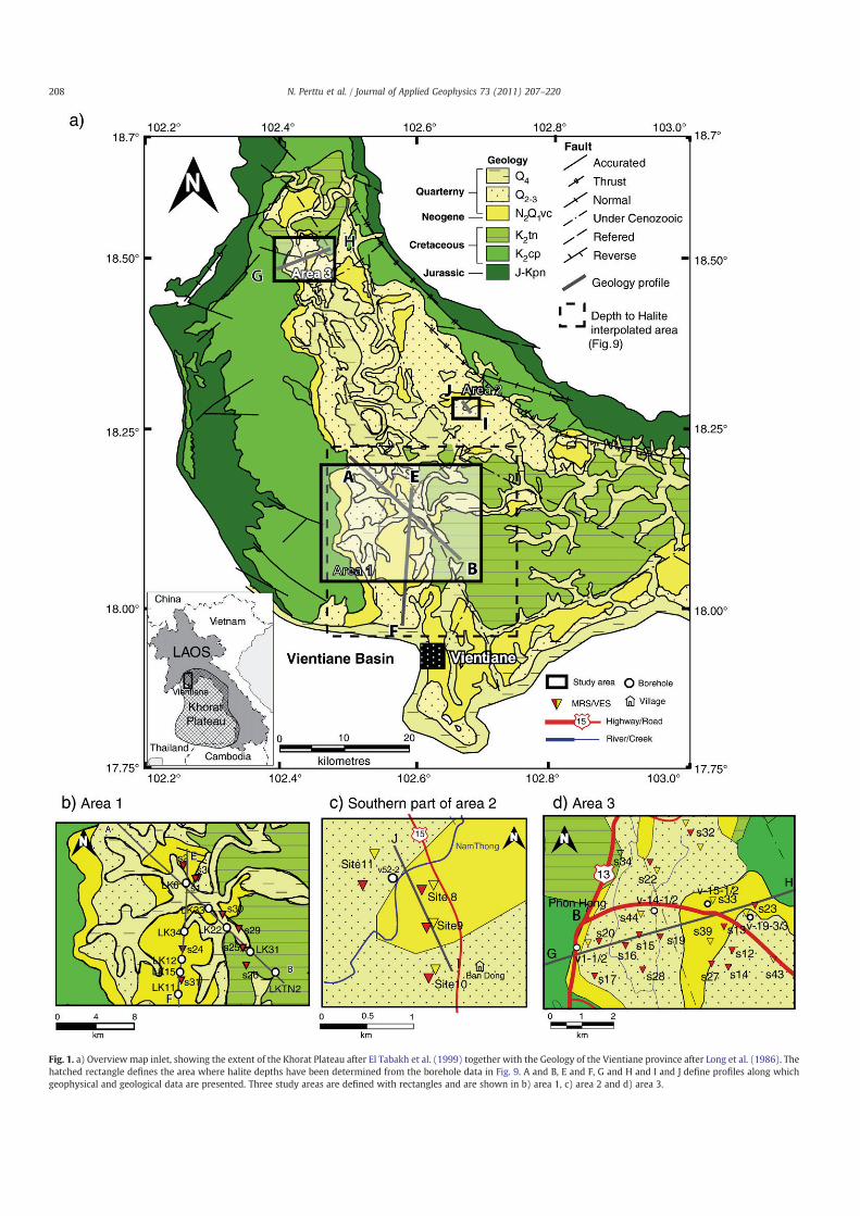
Fig. 1. a) Overview map inlet, showing the extent of the Khorat Plateau after El Tabakh et al. (1999) together with the Geology of the Vientiane province after Long et al. (1986). Thehatched rectangle defines the area where halite depths have been determined from the borehole data in Fig. 9. A and B, E and F, G and H and I and J define profiles along whichgeophysical and geological data are presented. Three study areas are defined with rectangles and are shown in b) area 1, c) area 2 and d) area 3.
208 N. Perttu et al. / Journal of Applied Geophysics 73 (2011) 207–220
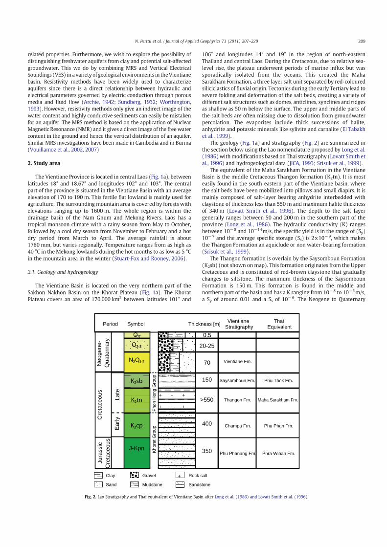
related properties. Furthermore, we wish to explore the possibility ofdistinguishing freshwater aquifers from clay and potential salt-affectedgroundwater. This we do by combining MRS and Vertical ElectricalSoundings (VES) in a varietyof geological environments in theVientianebasin. Resistivity methods have been widely used to characterizeaquifers since there is a direct relationship between hydraulic andelectrical parameters governed by electric conduction through porousmedia and fluid flow (Archie, 1942; Sundberg, 1932; Worthington,1993). However, resistivity methods only give an indirect image of thewater content and highly conductive sediments can easily be mistakenfor an aquifer. The MRS method is based on the application of NuclearMagnetic Resonance (NMR) and it gives a direct image of the freewatercontent in the ground and hence the vertical distribution of an aquifer.Similar MRS investigations have been made in Cambodia and in Burma(Vouillamoz et al., 2002, 2007)
2. Study area
The Vientiane Province is located in central Laos (Fig. 1a), betweenlatitudes 18° and 18.67° and longitudes 102° and 103°. The centralpart of the province is situated in the Vientiane Basin with an averageelevation of 170 to 190 m. This fertile flat lowland is mainly used foragriculture. The surrounding mountain area is covered by forests withelevations ranging up to 1600 m. The whole region is within thedrainage basin of the Nam Gnum and Mekong Rivers. Laos has atropical monsoon climate with a rainy season from May to October,followed by a cool dry season from November to February and a hotdry period from March to April. The average rainfall is about1780 mm, but varies regionally. Temperature ranges from as high as40 °C in the Mekong lowlands during the hot months to as low as 5 °Cin the mountain area in the winter (Stuart-Fox and Rooney, 2006).
2.1. Geology and hydrogeology
The Vientiane Basin is located on the very northern part of theSakhon Nakhon Basin on the Khorat Plateau (Fig. 1a). The KhoratPlateau covers an area of 170,000 km2 between latitudes 101° and
106° and longitudes 14° and 19° in the region of north-easternThailand and central Laos. During the Cretaceous, due to relative sea-level rise, the plateau underwent periods of marine influx but wassporadically isolated from the oceans. This created the MahaSarakham Formation, a three layer salt unit separated by red-colouredsiliciclastics of fluvial origin. Tectonics during the early Tertiary lead tosevere folding and deformation of the salt beds, creating a variety ofdifferent salt structures such as domes, anticlines, synclines and ridgesas shallow as 50 m below the surface. The upper and middle parts ofthe salt beds are often missing due to dissolution from groundwaterpercolation. The evaporites include thick successions of halite,anhydrite and potassic minerals like sylivite and carnalite (El Tabakhet al., 1999).
The geology (Fig. 1a) and stratigraphy (Fig. 2) are summarized inthe section below using the Lao nomenclature proposed by Long et al.(1986) withmodifications based on Thai stratigraphy (Lovatt Smith etal., 1996) and hydrogeological data (JICA, 1993; Srisuk et al., 1999).
The equivalent of the Maha Sarakham Formation in the VientianeBasin is the middle Cretaceous Thangon formation (K2tn). It is mosteasily found in the south-eastern part of the Vientiane basin, wherethe salt beds have been mobilized into pillows and small diapirs. It ismainly composed of salt-layer bearing anhydrite interbedded withclaystone of thickness less than 550 m and maximum halite thicknessof 340 m (Lovatt Smith et al., 1996). The depth to the salt layergenerally ranges between 50 and 200 m in the southern part of theprovince (Long et al., 1986). The hydraulic conductivity (K) rangesbetween 10−8 and 10−14m/s, the specific yield is in the range of (Sy)10−7 and the average specific storage (Ss) is 2x10⁻⁹, which makesthe Thangon Formation an aquiclude or non water-bearing formation(Srisuk et al., 1999).
The Thangon formation is overlain by the Saysomboun Formation(K2sb) (not shown onmap). This formation originates from the UpperCretaceous and is constituted of red-brown claystone that graduallychanges to siltstone. The maximum thickness of the SaysombounFormation is 150 m. This formation is found in the middle andnorthern part of the basin and has a K ranging from 10−8 to 10−5m/s,a Sy of around 0.01 and a Ss of 10−6. The Neogene to Quaternary
Neo
gene
-Q
uate
rnar
yC
reta
ceou
s
Ear
lyLa
te
Jura
ssic
Cre
tace
ous
J-Kpn
0.5
20-25
70
150
>550
400
350
Pho
n H
ong
Gro
upK
hora
t Gro
up
SymbolPeriod Thickness [m] VientianeStratigraphy
Vientiane Fm.
Saysomboun Fm.
Thangon Fm.
Champa Fm.
Phu Phanang Fm.
ThaiEquivalent
Phu Thok Fm.
Maha Sarakham Fm.
Phu Phan Fm.
Phra Wihan Fm.
Clay
Sand
Gravel
Mudstone
Rock salt
Sandstone
Fig. 2. Lao Stratigraphy and Thai equivalent of Vientiane Basin after Long et al. (1986) and Lovatt Smith et al. (1996).
209N. Perttu et al. / Journal of Applied Geophysics 73 (2011) 207–220
Vientiane Formation (N2Q1vc) has a thickness less than 70 m. Thisformation is overlain by stratigraphic units: Q2–3 (b25 m) and Q4
(b0.5 m) of Quaternary origin. N2Q1vc and Q2–3 are alluvial depositsfound in abandoned river channels and contain mostly gravel, sandand clay. Since they share the same characteristics they will bereferred to as the N2Q1–3 unit in this paper. The equivalent Thai unithas a K ranging from 10−6 to 10−4m/s, with Sy around 0.15 and Ssaround 2 to 3x10⁻³. The possibility of developing groundwater inthis unit is regarded as high (JICA, 1993). The above-mentioned unitsare all part of the Phon Hong Group. Underlying the ThangonFormation is the Khorat Group, which among others consists of theChampa- (K2cp) and Phu Pha Nang (J-Kpn) formations. These units,up to 400 m and 350 m thick, respectively, are found primarily in thewestern and eastern part of the basin. They are largely composed ofsandstone of Cretaceous and Jurassic age, with K ranging from 10−8 to10−5 m/s, Sy of around 0.05 and Ss of about 5x10⁻⁶.
2.2. Investigation areas
Three areas were selected for geophysical studies (Fig. 1a), witharea 1 located about 20 km north of Vientiane in the district ofThangon, area 2 located around 40 km northeast in the district ofTholakhom and area 3 located about 60 km northwest of Vientiane inthe district of Phon Hong. Data have been collected from 46 sites, 32MRS and 39 VES sites. The locations have been chosen according todifferences in geology, where geological data were retrieved from JICA(1993), (1994) and the Department of Geology and Mining inVientiane (Long et al., 1986). In an initial survey, noise level(b100 nV on noise analyzer), magnetic susceptibility (b10−3) of theupper soils and accessibility were evaluated, which in most casesresulted in dry rice paddies being chosen as measuring sites.
3. Geophysical methods and interpretation techniques
The MRS measurements in this study have been carried out withthe Numis-Plus equipment manufactured by Iris instruments. Themagnetic field was measured using a G 816 magnetometer (Geomet-rics) with a resolution of 1 nT. The VES measurements wereconducted with a Terrameter SAS4000 (ABEM). Resistivity measure-ments of core samples have been conducted in the geophysicallaboratory at Luleå University of Technology.
3.1. Magnetic Resonance Sounding (MRS)
MRS is a non invasive geophysical technique that energizes thehydrogen nuclei in the groundwater by transmitting an electromag-netic pulse at the Larmor frequency followed by a 30 ms dead time,when the instrument switches from transmitting to receiving mode.The resonance signal emitted by the hydrogen nucleus is thenrecorded. The method and principles are thoroughly described inLegchenko and Valla (2002), Lubczynski and Roy (2003) andYaramanci (2004). The initial amplitude (E0) of the received signalis directly related to the free water content (θMRS) and the transverserelaxation time T2* is a characteristic time for the loss of the spinrotation coherence and is directly linked to the mean pore size andmagnetic susceptibility of the water-filled pores. Typical values of T2*for different lithology classes are presented in Table 1 (Shirov et al.,1991). Fine sediments, such as clay with a highwater content but withmost of its water bound to the pore walls, or sediments with highmagnetic susceptibility cannot be detected due to shorter decay timesthan the current dead time limitation (30 ms) of the Numisequipment. The MRS water content is therefore related to the freewater content and should not be mistaken for the total water content.θMRS is determined from the inversion of E0 and is presented as afunction of θMRS, together with T2* versus depth.
In coarse grained aquifers, parameters such as porosity (η) andeffective porosity (ηe) can be roughly determined directly from theinversion of E0. This is under the assumption that bound water anddead-end, unconnected porosity is negligible (Lubczynski and Roy,2003). Assuming that θMRS reflects η, (θMRS≈η), the specific yield (Sy)or specific drainage (Sd) can be approximately estimated forunconfined, or respectively confined aquifers as:
Sy;d = θMRS−SR ð1Þ
where SR is the specific retention, which can be determined by othermethods (Lubczynski and Roy, 2003) or retrieved from tabled values(Table 1). In the confined aquifers, the specific storage (Ss) can becalculated from:
Ss = ρg α + θMRSβð Þ ð2Þ
where ρ is the density of water, g is the acceleration of gravity, α and βare the compressibilities of the aquifer andwater, respectively (Table 1).
The hydrostatic column (Hw) [m3/m2] gives a direct volumetricestimate of the free water content as a function of depth. This is themost reliable MRS parameter since it is less sensitive to equivalence,than the water content and thickness alone. It is here estimated for adepth extent, for which data are reliable.
HW = ∫Z max
Z min
θMRS⋅Δz: ð3Þ
Access to pumping test data makes it possible to relate T2* andθMRS to transmissivity (Legchenko et al., 2004) according to:
TMRS = CT ∫Δz
θa⋅T�22 ⋅dz ð4Þ
where CT is an area specific constant derived from pumping testtransmissivity (Tp) data:
CT = ∑n
i=1TP�i =∑
n
i=1ΔzMRSθ
aMRS⋅T�22 ð5Þ
and a usually takes the value 1 or 4.In our study, the geomagnetic field in the three areas had an
inclination of 24° and the field intensity varied between 43,620 and43,850 nT equivalent to a Larmor frequency of 1859 to 1868 Hz. Thisallowed notch filters to be used (F=50 Hz power line frequency),since there is little or no influence on the MRS signal when theharmonics of the power line frequency closest to the Larmorfrequency is greater than 8 Hz for a T2*=400 ms (Legchenko andValla, 2003). Depending on the noise amplitude, a 100 m square loopor an eight shaped loop with a 50 m side length was used togetherwith a signal stacking typically of 64 to 100 stacks.
Table 1Typical values of decay time (T2*) for different geological materials (Allen et al., 1997;Shirov et al., 1991). Values of specific retention (SR) after Hamill and Bell (1986),Johnson (1967) and Morris and Johnson (1967). Vertical compressibility (α) for somegeological materials and for water (β) (Domenico and Mifflin, 1965).
Decay time SR [%] α [m2/N] x10-8 Petrophysical information
T2*b3 ms 25–45 6.9–200 Clay bound waterT2* b30 ms Sandy clays30bT2* b60 5–15 1.3–10 Clay sands, very fine sands60bT2* b120 Fine sands120bT2* b180 Medium sands180bT2* b300 3–12 0.52–1 Coarse and gravely sands300bT2* b600 Gravel deposits600bT2* b1500 β [25°C]=4.8x10⁻¹⁰ Surface water bodies
210 N. Perttu et al. / Journal of Applied Geophysics 73 (2011) 207–220
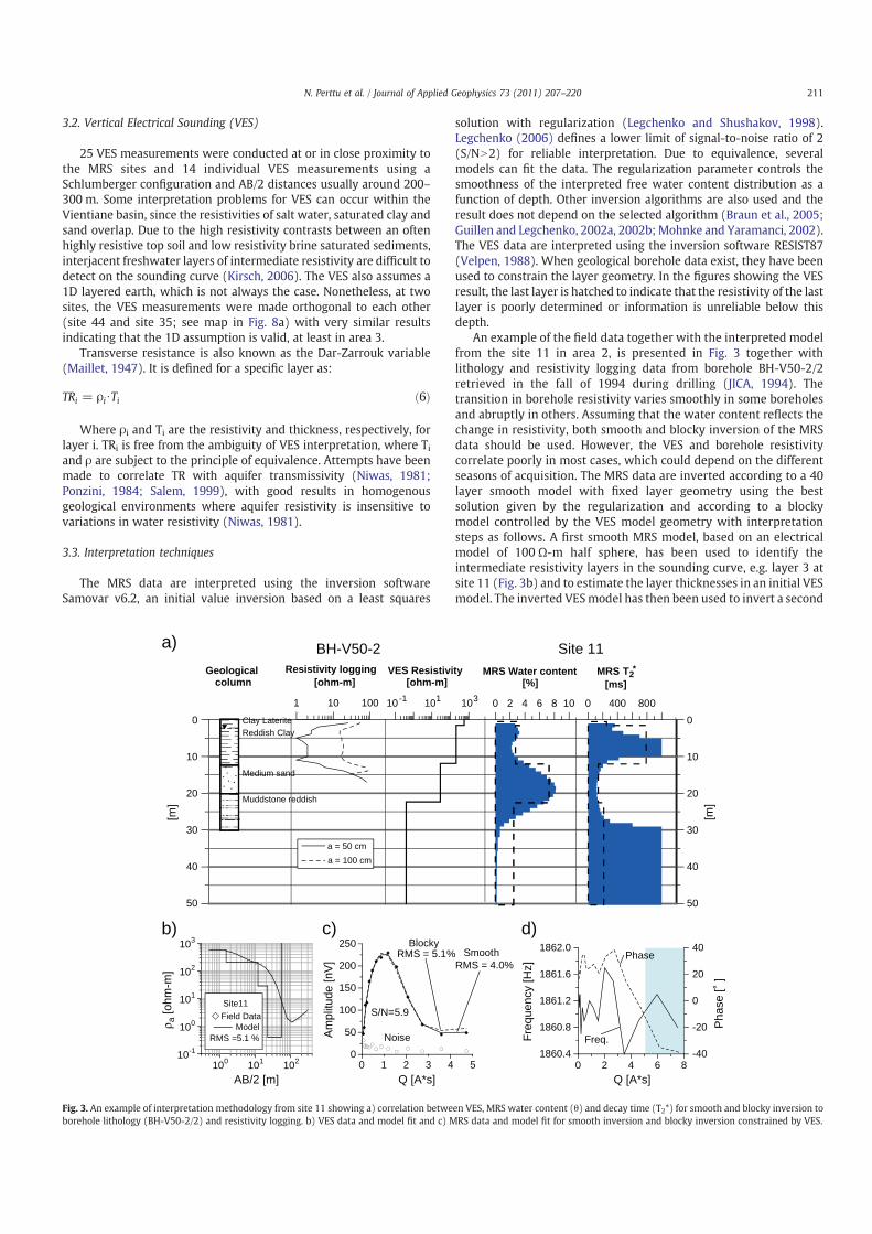
3.2. Vertical Electrical Sounding (VES)
25 VES measurements were conducted at or in close proximity tothe MRS sites and 14 individual VES measurements using aSchlumberger configuration and AB/2 distances usually around 200–300 m. Some interpretation problems for VES can occur within theVientiane basin, since the resistivities of salt water, saturated clay andsand overlap. Due to the high resistivity contrasts between an oftenhighly resistive top soil and low resistivity brine saturated sediments,interjacent freshwater layers of intermediate resistivity are difficult todetect on the sounding curve (Kirsch, 2006). The VES also assumes a1D layered earth, which is not always the case. Nonetheless, at twosites, the VES measurements were made orthogonal to each other(site 44 and site 35; see map in Fig. 8a) with very similar resultsindicating that the 1D assumption is valid, at least in area 3.
Transverse resistance is also known as the Dar-Zarrouk variable(Maillet, 1947). It is defined for a specific layer as:
TRi = ρi⋅Ti ð6Þ
Where ρi and Ti are the resistivity and thickness, respectively, forlayer i. TRi is free from the ambiguity of VES interpretation, where Tiand ρ are subject to the principle of equivalence. Attempts have beenmade to correlate TR with aquifer transmissivity (Niwas, 1981;Ponzini, 1984; Salem, 1999), with good results in homogenousgeological environments where aquifer resistivity is insensitive tovariations in water resistivity (Niwas, 1981).
3.3. Interpretation techniques
The MRS data are interpreted using the inversion softwareSamovar v6.2, an initial value inversion based on a least squares
solution with regularization (Legchenko and Shushakov, 1998).Legchenko (2006) defines a lower limit of signal-to-noise ratio of 2(S/NN2) for reliable interpretation. Due to equivalence, severalmodels can fit the data. The regularization parameter controls thesmoothness of the interpreted free water content distribution as afunction of depth. Other inversion algorithms are also used and theresult does not depend on the selected algorithm (Braun et al., 2005;Guillen and Legchenko, 2002a, 2002b; Mohnke and Yaramanci, 2002).The VES data are interpreted using the inversion software RESIST87(Velpen, 1988). When geological borehole data exist, they have beenused to constrain the layer geometry. In the figures showing the VESresult, the last layer is hatched to indicate that the resistivity of the lastlayer is poorly determined or information is unreliable below thisdepth.
An example of the field data together with the interpreted modelfrom the site 11 in area 2, is presented in Fig. 3 together withlithology and resistivity logging data from borehole BH-V50-2/2retrieved in the fall of 1994 during drilling (JICA, 1994). Thetransition in borehole resistivity varies smoothly in some boreholesand abruptly in others. Assuming that the water content reflects thechange in resistivity, both smooth and blocky inversion of the MRSdata should be used. However, the VES and borehole resistivitycorrelate poorly in most cases, which could depend on the differentseasons of acquisition. The MRS data are inverted according to a 40layer smooth model with fixed layer geometry using the bestsolution given by the regularization and according to a blockymodel controlled by the VES model geometry with interpretationsteps as follows. A first smooth MRS model, based on an electricalmodel of 100 Ω-m half sphere, has been used to identify theintermediate resistivity layers in the sounding curve, e.g. layer 3 atsite 11 (Fig. 3b) and to estimate the layer thicknesses in an initial VESmodel. The inverted VESmodel has then been used to invert a second
50
40
30
20
10
0[m
]
50
40
30
20
10
0
[m]
Clay LateriteReddish Clay
Medium sand
Muddstone reddish
Geologicalcolumn
0 100
[ohm-m]
10-1 101 103
VES Resistivity [ohm-m]
0
MRS Water content[%]
1 1 0 2 4 6 8 1 0 400 800
MRS T2*
[ms]
BH-V50-2 Site 11
a = 50 cm a = 100 cm
Resistivity logging
100 101 102
AB/2 [m]
10-1
100
101
102
103
ρ a [o
hm-m
]
Field Data
RMS =5.1 %
Site11
Model
0 2 31 4 50
50
100
150
200
250RMS = 5.1%
RMS = 4.0%
S/N=5.9
Q [A*s]
Am
plitu
de [n
V]
BlockySmooth
Noise
a)
b) c)
1860.4
1860.8
1861.2
1861.6
1862.0
Freq
uenc
y [H
z]
-40
-20
0
20
40
Pha
se [˚
]
Q [A*s]
d)
Freq.
Phase
0 4 62 8
Fig. 3. An example of interpretation methodology from site 11 showing a) correlation between VES, MRS water content (θ) and decay time (T2*) for smooth and blocky inversion toborehole lithology (BH-V50-2/2) and resistivity logging. b) VES data and model fit and c) MRS data and model fit for smooth inversion and blocky inversion constrained by VES.
211N. Perttu et al. / Journal of Applied Geophysics 73 (2011) 207–220
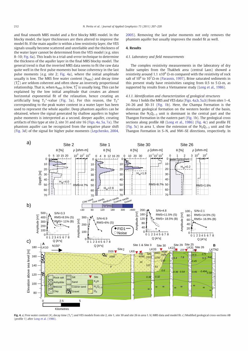
and final smooth MRS model and a first blocky MRS model. In theblocky model, the layer thicknesses are then altered to improve themodel fit. If the main aquifer is within a low resistivity layer, the VESsignals usually become scattered and unreliable and the thickness ofthe water layer cannot be determined from the VES model (e.g. sites8–10; Fig. 6a). This leads to a trial-and-error technique to determinethe thickness of the aquifer layer in the final MRS blocky model. Thegeneral trend is that the inverted MRS data seems to fit the raw dataquite well in the first pulse moments but loose coherency in the lastpulse moments (e.g. site 2; Fig. 4a), where the initial amplitudeusually is low. The MRS free water content (θMRS) and decay time(T2⁎) are seldom coherent and often show an inversely proportionalrelationship. That is, when θMRS is low, T2⁎ is usually long. This can beexplained by the low initial amplitude that creates an almosthorizontal exponential fit of the relaxation, hence creating anartificially long T2*-value (Fig. 3a). For this reason, the T2*corresponding to the peak water content in a water layer has beenused to represent the whole aquifer. Deep phantom aquifers can beobtained, where the signal generated by shallow aquifers in higherpulse moments is interpreted as a second, deeper aquifer, creatingartifacts of this type at site 2, site 31 and site 16 (Figs. 4a, 5a, 7a). Thephantom aquifer can be recognized from the negative phase shift(Fig. 3d) of the signal for higher pulse moments (Legchenko, 2004,
2005). Removing the last pulse moments not only removes thephantom aquifer but usually improves the model fit as well.
4. Results
4.1. Laboratory and field measurements
The complex resistivity measurements in the laboratory of dryhalite samples from the Thakhek area (central Laos) showed aresistivity around 1.1 x10⁶ Ω-m compared with the resistivity of rocksalt of 106 to 107Ω-m (Parasnis, 1997). Brine saturated sediments inthis present study have resistivities ranging from 0.5 to 5 Ω-m, assupported by results from a Vietnamese study (Long et al., 1986).
4.1.1. Identification and characterization of geological structuresArea 1 holds the MRS and VES data (Figs. 4a,b, 5a,b) from sites 1–4,
24–26 and 30–31 (Fig. 1b). Here, the Champa Formation is thedominant geological formation on the western border of the basin,whereas the N2Q1–3 unit is dominant in the central part and theThangon Formation in the eastern part (Fig. 1b). The geological crosssections along profile AB (Long et al., 1986) (Fig. 4c) and profile FE(Fig. 5c) in area 1, show the extension of the N2Q1–3 unit and theThangon Formation in S–N, and NW–SE directions, respectively. In
0 10 15 20
70
60
50
40
30
20
10
0100 102 104
θ [%] ρ [ohm-m]
0 4 8 12 16 20
70
60
50
40
30
20
10
0
θ [%]0 10 20 30
70
60
50
40
30
20
10
010-1101103
θ [%] ρ [ohm-m]0 1 2 3
70
60
50
40
30
20
10
0100 102
θ [%] ρ [ohm-m]Site 2 Site 1 Site 30 Site 26a)
Dep
th [m
]
S/N=3.3RMS=8.5% (S)RMS= 11% (B)
S/N=6.9RMS=6% (S)
S/N=4.8RMS=11.5% (S)RMS= 18.5% (B)
S/N=2.1RMS=14.5% (S)RMS= 16.9% (B)
Hw=4.0
Hw=2.9
Hw=1.9
Hw=0.2
RMS=4.7% RMS=8.7% RMS=1.6%
Q4
LK10LK6
LK33 LK22 LK31LKTN2
A BSite2
Site 1 & Site 3
170
6.8
0.58
175
5.3
0.494
190
14.6
0.45
0.45
220
7.8
0.54
100
5.4
0.36
45001928
233
0.6
4400
1100
63
0.32
5801513
122
0.38
5315150
19
1560
9
8
8 8 8 8 8
8
8
Site 30 Site 29 Site 25
2939Site 26
Ele
vatio
n ab
ove
sea
leve
l [m
]
80
180
160
140
120
100
Q [A*s]
04080
120160200
Am
plitu
de [n
V]
1 2 3 4 5 6 7 80
Q [A*s]
0
100
200
300
Am
plitu
de [n
V]
1 2 3 4 5 6 7 80
0100200300400500
Am
plitu
de [n
V]
Q [A*s] 1 2 3 4 5 6 7 80
020406080
100
Am
plitu
de [n
V]
Q [A*s] 1 2 3 4 5 6 7 80
≤30 120 30060 180 ≥600
Clay sandFine sands
Medium sandsCoarse sands
Gravel
T2 [ms]
N150°
0 2.5 5
Kilometres
Anhydrite
Rock salt
Breccia
Clay
Silt
Sand
Coarse sand
Gravel
K2tn
N2Q1-3
Q4
Site
b)
c)
FID1Noise
5
Fig. 4. a) Free water content (θ), decay time (T2*) and VES models from site 2, site 1, site 30 and site 26 in area 1. b) MRS data and model fit. c) Modified geological cross-sections AB(profile 1) after Long et al. (1986).
212 N. Perttu et al. / Journal of Applied Geophysics 73 (2011) 207–220
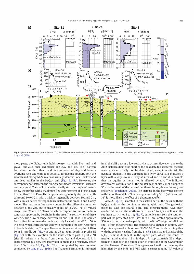
most parts, the N2Q1–3 unit holds coarser materials like sand andgravel but also finer sediments like clay and silt. The ThangonFormation on the other hand, is composed of clay and brecciaoverlying rock salt, with poor potential for hosting aquifers. Both thesmooth and blocky MRS inversion usually identifies one shallow andone deep aquifer in the N2Q1–3 unit (Figs. 4a, 5a). However, thecorrespondence between the blocky and smooth inversions is usuallynot very good. The shallow aquifer usually starts a couple of metersbelow the surfacewith amaximum freewater content of 4 to 6% downto a depth of 10 to 15 m. The deeper aquifer generally starts at a depthof around 10 to 30 mwith a thickness generally between 10 and 30 m,with a much better correspondence between the smooth and blockymodel. The maximum free water content for the different sites variesbetween 5 and 25%, but is usually about 10 to 20%. The T2*-valuesrange from 70 ms to 150 ms, which correspond to fine to mediumsands as supported by boreholes in the area. The resistivities of thesewater-bearing layers range between 10 and 1500 Ω-m. The aquiferfloor differs from site to site but it is usually located around 20 to 50 min depth, which corresponds well with borehole lithology. Accordingto borehole data, the Thangon Formation is located at depths of 40 to50 m in profile AB (Fig. 4c) and at 25 to 50 m depth in profile FE(Fig. 5c), with the exception for the south-eastern part in profile AB(site 26) where it is found from the surface and downward. It ischaracterized by a very low free water content and a resistivity lowerthan 5 Ω-m (site 26; Fig. 4a). This is supported by measurementconducted by Long et al. (1986). The Thangon Formation is indicated
in all the VES data as a low resistivity structure. However, due to theAB/2 distances being too short or the field data too scattered, the trueresistivity can usually not be determined, except in site 26. Thenegative gradient in the apparent resistivity curve still indicates alayer with a very low resistivity at sites 24 and 30 and it is possiblethat the aquifer at these sites is affected by salt. The indicateddownwards continuation of the aquifer (e.g. at site 24) at a depth of30 m is the result of the reduced depth resolution, due to the very lowresistivity (Legchenko, 2008). The increase in the free water contentin the smooth model (N2%) at a depth exceeding 50 m (site 2 and site31) is most likely the effect of a phantom aquifer.
Area 2 (Fig. 1c) is located in the eastern part of the basin, with theN2Q1–3 unit as the dominating stratigraphic unit. The geologicalborehole data are sparse here. The measurements have beenconducted both in the northern part (sites 5 to 7) as well as in thesouthern part (sites 8 to 11; Fig. 7), but only sites from the southernpart will be presented here. Sites 8 to 11 are located approximately500 m apart on a large rice paddy, with the Nam Thong creek dividingsite 11 from the other sites. The compositional change in geology withdepth is expressed in borehole BH-V-52-2/2 and is shown togetherwith the geophysical data from site 11 (Fig. 3a). Clay and laterite of theN2Q1–3 unit is dominant in the upper part, which transcends tomedium sand at about 13 m in depth. At approximately 22 m depththere is a change in the composition to mudstone of the Saysombounor the Thangon Formation. This agrees well with the main aquiferidentified by the MRS and VES with a corresponding T2* value of
N2Q1-3
Q4
LK8LK11 LK15 LK12
LK34 LK6
FE
Site 2 Site1 & Site 3 Site 24Site31
8
8
8 8
9003300
14
80
900
0.2
5005200
19
2940
1560
9
Ele
vatio
n ab
ove
sea
leve
l [m
]
200
180
160
140
120
100
80
101 103
ρ [ohm-m]Site 31 Site 24 Site 3
70
60
50
40
30
20
10
0101 103
θ [%] ρ [ohm-m]
0 0 10 202 4 6 8 0 4 8 1210
70
60
50
40
30
20
10
0
θ [%]
60
50
40
30
20
10
010-1 101 103
θ [%] ρ [ohm-m]
04080
120160200
Am
plitu
de [n
V]
FID1Noise
Dep
th [m
]
70
0
100
200
300
Am
plitu
de [n
V]
Q [A*s]
0
100
200
300
400
Am
plitu
de [n
V]
1 80Q [A*s]
1 80Q [A*s]
1 2 3 4 5 6 7 2 3 4 5 6 7 2 3 4 5 6 780
S/N=2.4RMS=7.1% (S)RMS= 9.2% (B)
S/N=2.5RMS=8.8% (S)RMS= 9.1% (B)
S/N=3.4RMS=14.4% (S)RMS= 16.1% (B)
50 2.5
Kilometers
N5°
a)
b)
c)
Hw=1.2Hw=3.8
Hw=3.7
≤30
60
120
180
300
≥600
Clay sandFine sandsM
edium sands
Coarse sands
Gravel
T2 [ms]RMS=3.2% RMS=8.6% RMS=2.8%
Anhydrite
Rock salt
Breccia
Clay
Silt
Sand
Coarse sand
Gravel
K2tn
N2Q1-3
Q4
Site
K2tn
Fig. 5. a) Freewater content (θ), decay time (T2*) andVESmodels fromsite31, site 24and site 3 inarea1. b)MRSdata andmodelfit. c)Modifiedgeological cross sectionsAB(profile 1) afterLong et al. (1986).
213N. Perttu et al. / Journal of Applied Geophysics 73 (2011) 207–220
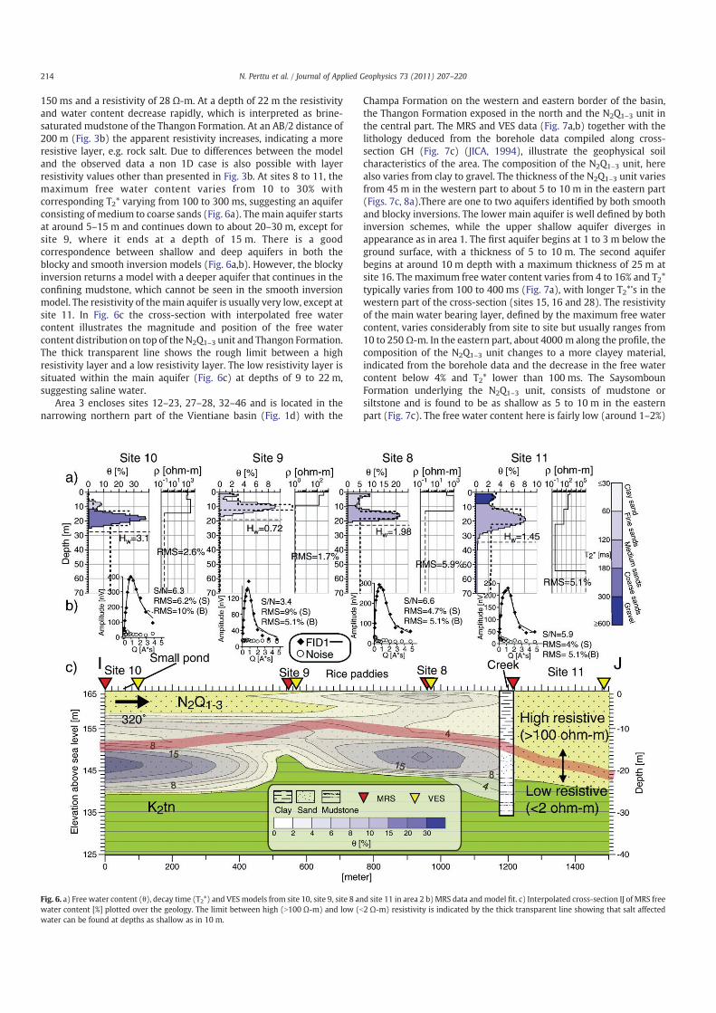
150 ms and a resistivity of 28 Ω-m. At a depth of 22 m the resistivityand water content decrease rapidly, which is interpreted as brine-saturated mudstone of the Thangon Formation. At an AB/2 distance of200 m (Fig. 3b) the apparent resistivity increases, indicating a moreresistive layer, e.g. rock salt. Due to differences between the modeland the observed data a non 1D case is also possible with layerresistivity values other than presented in Fig. 3b. At sites 8 to 11, themaximum free water content varies from 10 to 30% withcorresponding T2* varying from 100 to 300 ms, suggesting an aquiferconsisting of medium to coarse sands (Fig. 6a). Themain aquifer startsat around 5–15 m and continues down to about 20–30 m, except forsite 9, where it ends at a depth of 15 m. There is a goodcorrespondence between shallow and deep aquifers in both theblocky and smooth inversion models (Fig. 6a,b). However, the blockyinversion returns a model with a deeper aquifer that continues in theconfining mudstone, which cannot be seen in the smooth inversionmodel. The resistivity of themain aquifer is usually very low, except atsite 11. In Fig. 6c the cross-section with interpolated free watercontent illustrates the magnitude and position of the free watercontent distribution on top of the N2Q1–3 unit and Thangon Formation.The thick transparent line shows the rough limit between a highresistivity layer and a low resistivity layer. The low resistivity layer issituated within the main aquifer (Fig. 6c) at depths of 9 to 22 m,suggesting saline water.
Area 3 encloses sites 12–23, 27–28, 32–46 and is located in thenarrowing northern part of the Vientiane basin (Fig. 1d) with the
Champa Formation on the western and eastern border of the basin,the Thangon Formation exposed in the north and the N2Q1–3 unit inthe central part. The MRS and VES data (Fig. 7a,b) together with thelithology deduced from the borehole data compiled along cross-section GH (Fig. 7c) (JICA, 1994), illustrate the geophysical soilcharacteristics of the area. The composition of the N2Q1–3 unit, herealso varies from clay to gravel. The thickness of the N2Q1–3 unit variesfrom 45 m in the western part to about 5 to 10 m in the eastern part(Figs. 7c, 8a).There are one to two aquifers identified by both smoothand blocky inversions. The lower main aquifer is well defined by bothinversion schemes, while the upper shallow aquifer diverges inappearance as in area 1. The first aquifer begins at 1 to 3 m below theground surface, with a thickness of 5 to 10 m. The second aquiferbegins at around 10 m depth with a maximum thickness of 25 m atsite 16. The maximum free water content varies from 4 to 16% and T2*typically varies from 100 to 400 ms (Fig. 7a), with longer T2*'s in thewestern part of the cross-section (sites 15, 16 and 28). The resistivityof the main water bearing layer, defined by the maximum free watercontent, varies considerably from site to site but usually ranges from10 to 250 Ω-m. In the eastern part, about 4000 m along the profile, thecomposition of the N2Q1–3 unit changes to a more clayey material,indicated from the borehole data and the decrease in the free watercontent below 4% and T2* lower than 100 ms. The SaysombounFormation underlying the N2Q1–3 unit, consists of mudstone orsiltstone and is found to be as shallow as 5 to 10 m in the easternpart (Fig. 7c). The free water content here is fairly low (around 1–2%)
Fig. 6. a) Free water content (θ), decay time (T2*) and VESmodels from site 10, site 9, site 8 and site 11 in area 2 b)MRS data andmodel fit. c) Interpolated cross-section IJ of MRS freewater content [%] plotted over the geology. The limit between high (N100 Ω-m) and low (b2 Ω-m) resistivity is indicated by the thick transparent line showing that salt affectedwater can be found at depths as shallow as in 10 m.
214 N. Perttu et al. / Journal of Applied Geophysics 73 (2011) 207–220
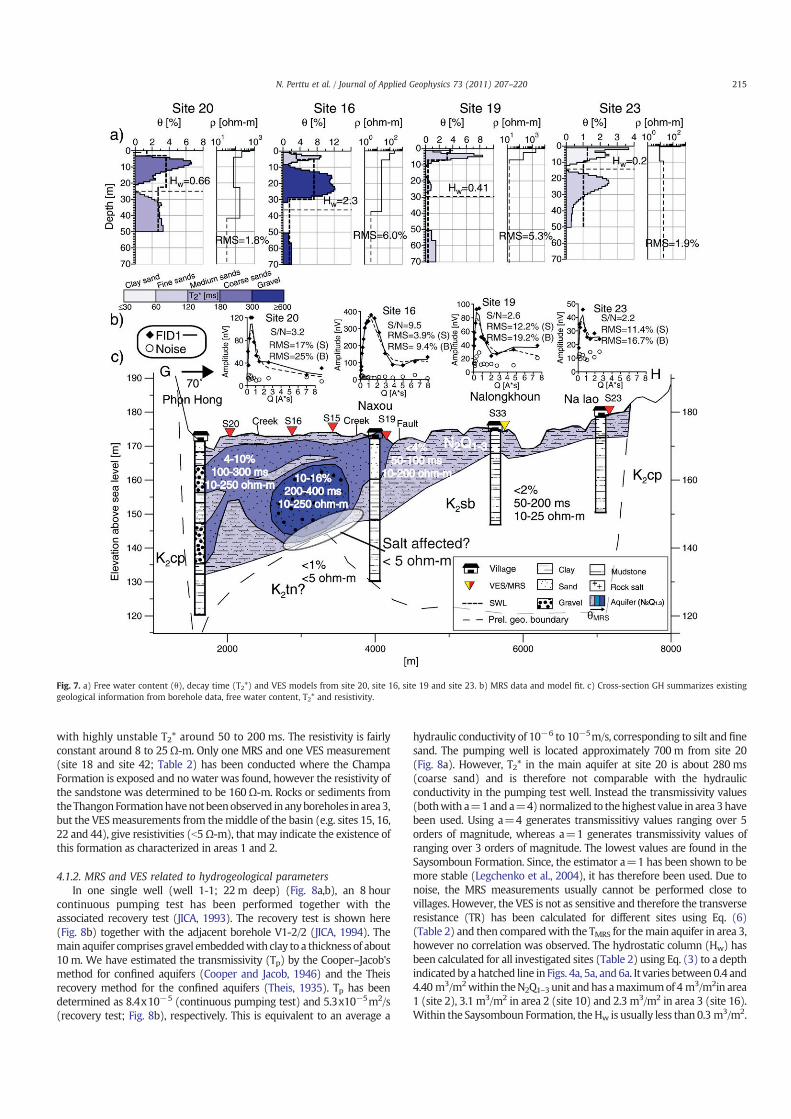
with highly unstable T2* around 50 to 200 ms. The resistivity is fairlyconstant around 8 to 25Ω-m. Only one MRS and one VES measurement(site 18 and site 42; Table 2) has been conducted where the ChampaFormation is exposed and no water was found, however the resistivity ofthe sandstone was determined to be 160Ω-m. Rocks or sediments fromtheThangonFormationhavenotbeenobserved inanyboreholes inarea3,but the VESmeasurements from themiddle of the basin (e.g. sites 15, 16,22 and 44), give resistivities (b5Ω-m), that may indicate the existence ofthis formation as characterized in areas 1 and 2.
4.1.2. MRS and VES related to hydrogeological parametersIn one single well (well 1-1; 22 m deep) (Fig. 8a,b), an 8 hour
continuous pumping test has been performed together with theassociated recovery test (JICA, 1993). The recovery test is shown here(Fig. 8b) together with the adjacent borehole V1-2/2 (JICA, 1994). Themain aquifer comprises gravel embeddedwith clay to a thickness of about10 m. We have estimated the transmissivity (Tp) by the Cooper–Jacob'smethod for confined aquifers (Cooper and Jacob, 1946) and the Theisrecovery method for the confined aquifers (Theis, 1935). Tp has beendetermined as 8.4x10⁻⁵ (continuous pumping test) and 5.3x10⁻⁵m2/s(recovery test; Fig. 8b), respectively. This is equivalent to an average a
hydraulic conductivity of 10−6 to 10−5m/s, corresponding to silt and finesand. The pumping well is located approximately 700 m from site 20(Fig. 8a). However, T2* in the main aquifer at site 20 is about 280 ms(coarse sand) and is therefore not comparable with the hydraulicconductivity in the pumping test well. Instead the transmissivity values(bothwith a=1and a=4)normalized to the highest value in area 3havebeen used. Using a=4 generates transmissitivy values ranging over 5orders of magnitude, whereas a=1 generates transmissivity values ofranging over 3 orders of magnitude. The lowest values are found in theSaysomboun Formation. Since, the estimator a=1 has been shown to bemore stable (Legchenko et al., 2004), it has therefore been used. Due tonoise, the MRS measurements usually cannot be performed close tovillages. However, the VES is not as sensitive and therefore the transverseresistance (TR) has been calculated for different sites using Eq. (6)(Table 2) and then comparedwith the TMRS for themain aquifer in area 3,however no correlation was observed. The hydrostatic column (Hw) hasbeen calculated for all investigated sites (Table 2) using Eq. (3) to a depthindicated by ahatched line in Figs. 4a, 5a, and6a. It varies between0.4 and4.40 m3/m2within theN2Q1–3 unit andhas amaximumof 4 m3/m2in area1 (site 2), 3.1 m3/m2 in area 2 (site 10) and 2.3 m3/m2 in area 3 (site 16).Within the Saysomboun Formation, theHw is usually less than 0.3 m3/m2.
Fig. 7. a) Free water content (θ), decay time (T2*) and VES models from site 20, site 16, site 19 and site 23. b) MRS data and model fit. c) Cross-section GH summarizes existinggeological information from borehole data, free water content, T2* and resistivity.
215N. Perttu et al. / Journal of Applied Geophysics 73 (2011) 207–220
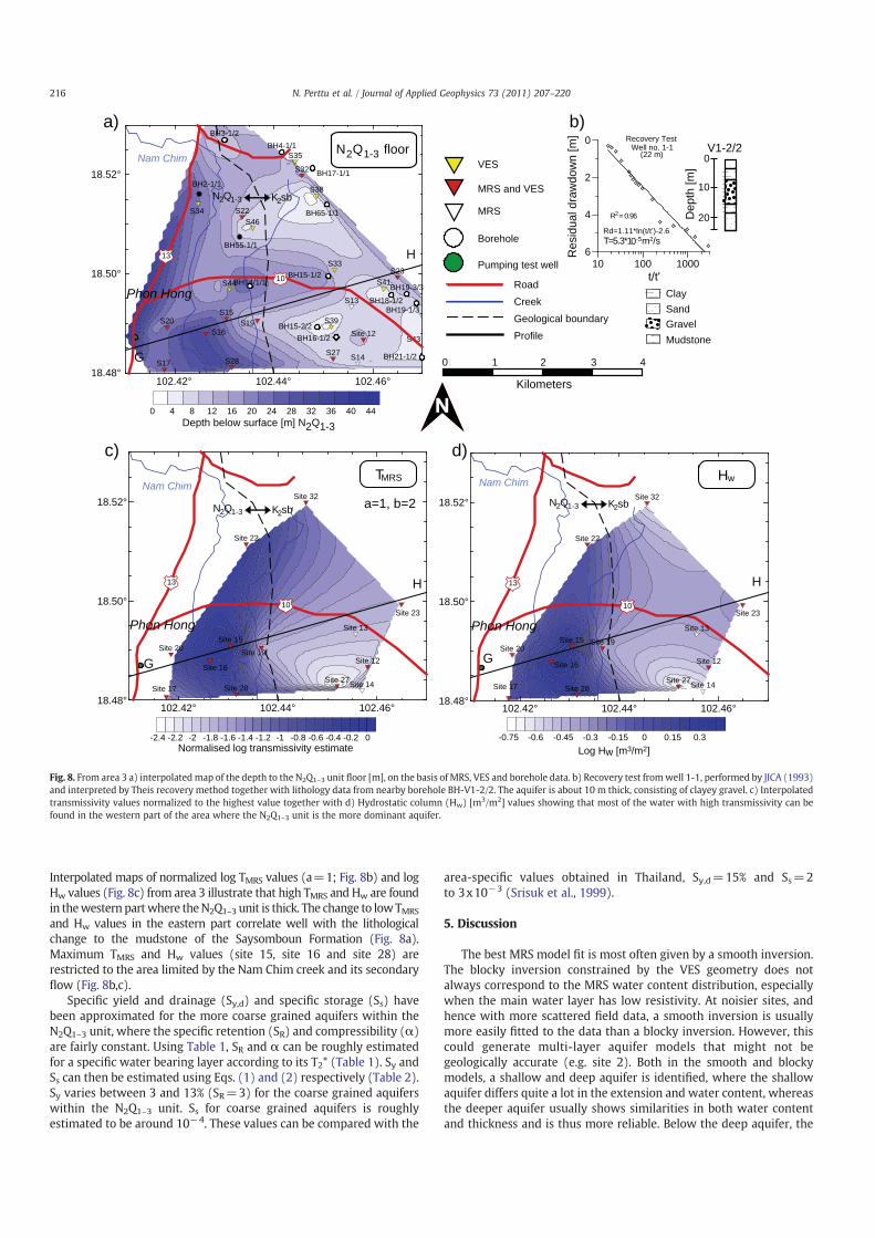
Interpolated maps of normalized log TMRS values (a=1; Fig. 8b) and logHw values (Fig. 8c) from area 3 illustrate that high TMRS and Hw are foundin thewestern partwhere theN2Q1–3 unit is thick. The change to lowTMRS
and Hw values in the eastern part correlate well with the lithologicalchange to the mudstone of the Saysomboun Formation (Fig. 8a).Maximum TMRS and Hw values (site 15, site 16 and site 28) arerestricted to the area limited by the Nam Chim creek and its secondaryflow (Fig. 8b,c).
Specific yield and drainage (Sy,d) and specific storage (Ss) havebeen approximated for the more coarse grained aquifers within theN2Q1–3 unit, where the specific retention (SR) and compressibility (α)are fairly constant. Using Table 1, SR and α can be roughly estimatedfor a specific water bearing layer according to its T2* (Table 1). Sy andSs can then be estimated using Eqs. (1) and (2) respectively (Table 2).Sy varies between 3 and 13% (SR=3) for the coarse grained aquiferswithin the N2Q1–3 unit. Ss for coarse grained aquifers is roughlyestimated to be around 10−4. These values can be compared with the
area-specific values obtained in Thailand, Sy,d=15% and Ss=2to 3x10⁻³ (Srisuk et al., 1999).
5. Discussion
The best MRS model fit is most often given by a smooth inversion.The blocky inversion constrained by the VES geometry does notalways correspond to the MRS water content distribution, especiallywhen the main water layer has low resistivity. At noisier sites, andhence with more scattered field data, a smooth inversion is usuallymore easily fitted to the data than a blocky inversion. However, thiscould generate multi-layer aquifer models that might not begeologically accurate (e.g. site 2). Both in the smooth and blockymodels, a shallow and deep aquifer is identified, where the shallowaquifer differs quite a lot in the extension and water content, whereasthe deeper aquifer usually shows similarities in both water contentand thickness and is thus more reliable. Below the deep aquifer, the
102.42° 102.44° 102.46°18.48°
18.50°
18.52°
0 4 8 12 16 20 24 28 32 36 40 44Depth below surface [m] N2Q1-3
MRS and VES
MRS
Borehole
Pumping test well
RoadCreekGeological boundary
VES
Profile
102.42° 102.44° 102.46°18.48°
18.50°
18.52°
Normalised log transmissivity estimate-2.4 -2.2 -2 -1.8 -1.6 -1.4 -1.2 -1 -0.8 -0.6 -0.4 -0.2 0
102.42° 102.44° 102.46°18.48°
18.50°
18.52°
-0.75 -0.6 -0.45 -0.3 -0.15 0 0.15 0.3Log Hw [m3/m2]
a) b)
c)
Kilometers
0 1 2 3 4
N
10 100 1000t/t'
6
4
2
0
R2= 0.96
Recovery TestWell no. 1-1
(22 m)
T=5.3*10-5m2/s
Res
idua
l dra
wdo
wn
[m]
Rd=1.11*ln(t/t’)-2.6
d)
0
10
20
V1-2/2
Dep
th [m
]
ClaySandGravelMudstone
Site 12
S13
S14
S15
S16
S17
S19S20
S22
S23
S27S28
S32
S33
S34
S35
S38
S39
S41
S43
S44
S46
BH17-1/1
BH3-1/2
BH2-1/1
BH15-2/2
BH15-1/2
BH65-1/1
BH18-1/2
BH21-1/2
BH55-1/1
BH14/1/1
BH16-1/2
BH19-3/3
BH19-1/3
13
10
Phon Hong
G
H
Nam ChimBH4-1/1
N2Q1-3 K2sb
N2Q1-3 floor
Site 12
Site 13
Site 14
Site 15
Site 16
Site 17
Site 19Site 20
Site 22
Site 23
Site 27Site 28
Site 32
Phon Hong
G
H13
Nam Chim
N2Q1-3 K2sb a=1, b=2
TMRS
10
N2Q1-3 K2sb
Hw
Site 12
Site 13
Site 14
Site 15
Site 16
Site 17
Site 19Site 20
Site 23
Site 27Site 28
Site 32
G
H13
10
Nam Chim
Site 22
Phon Hong
Fig. 8. From area 3 a) interpolatedmap of the depth to the N2Q1–3 unit floor [m], on the basis of MRS, VES and borehole data. b) Recovery test fromwell 1-1, performed by JICA (1993)and interpreted by Theis recovery method together with lithology data from nearby borehole BH-V1-2/2. The aquifer is about 10 m thick, consisting of clayey gravel. c) Interpolatedtransmissivity values normalized to the highest value together with d) Hydrostatic column (Hw) [m3/m2] values showing that most of the water with high transmissivity can befound in the western part of the area where the N2Q1–3 unit is the more dominant aquifer.
216 N. Perttu et al. / Journal of Applied Geophysics 73 (2011) 207–220
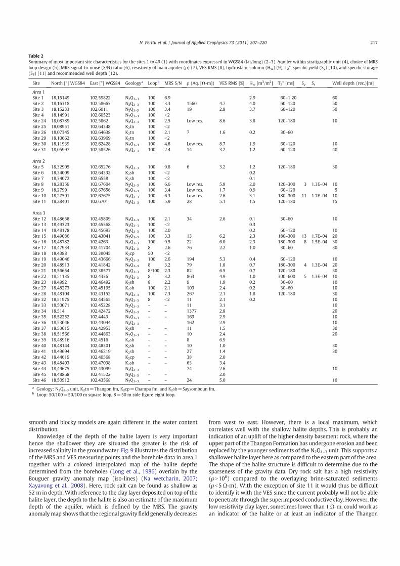
smooth and blocky models are again different in the water contentdistribution.
Knowledge of the depth of the halite layers is very importanthence the shallower they are situated the greater is the risk ofincreased salinity in the groundwater. Fig. 9 illustrates the distributionof the MRS and VES measuring points and the borehole data in area 1together with a colored interpolated map of the halite depthsdetermined from the boreholes (Long et al., 1986) overlain by theBouguer gravity anomaly map (iso-lines) (Na wetcharin, 2007;Xayavong et al., 2008). Here, rock salt can be found as shallow as52 m in depth.With reference to the clay layer deposited on top of thehalite layer, the depth to the halite is also an estimate of themaximumdepth of the aquifer, which is defined by the MRS. The gravityanomalymap shows that the regional gravity field generally decreases
from west to east. However, there is a local maximum, whichcorrelates well with the shallow halite depths. This is probably anindication of an uplift of the higher density basement rock, where theupper part of the Thangon Formation has undergone erosion and beenreplaced by the younger sediments of the N2Q1–3 unit. This supports ashallower halite layer here as compared to the eastern part of the area.The shape of the halite structure is difficult to determine due to thesparseness of the gravity data. Dry rock salt has a high resistivity(ρN106) compared to the overlaying brine-saturated sediments(ρb5 Ω-m). With the exception of site 11 it would thus be difficultto identify it with the VES since the current probably will not be ableto penetrate through the superimposed conductive clay. However, thelow resistivity clay layer, sometimes lower than 1 Ω-m, could work asan indicator of the halite or at least an indicator of the Thangon
Table 2Summary of most important site characteristics for the sites 1 to 46 (1) with coordinates expressed in WGS84 (lat/long) (2–3). Aquifer within stratigraphic unit (4), choice of MRSloop design (5), MRS signal-to-noise (S/N) ratio (6), resistivity of main aquifer (ρ) (7), VES RMS (8), hydrostatic column (Hw) (9), T2*, specific yield (Sy) (10), and specific storage(SS) (11) and recommended well depth (12).
Site North [°] WGS84 East [°] WGS84 Geologya Loopb MRS S/N ρ (Aq. [Ω-m]) VES RMS [%] Hw [m3/m2] T2* [ms] Sy Ss Well depth (rec.)[m]
Area 1Site 1 18,15149 102,59822 N2Q1–3 100 6.9 2.9 60–1 20 60Site 2 18,16318 102,58663 N2Q1–3 100 3.3 1560 4.7 4.0 60–120 50Site 3 18,15233 102,6011 N2Q1–3 100 3.4 19 2.8 3.7 60–120 50Site 4 18,14991 102,60523 N2Q1–3 100 b2Site 24 18,08789 102,5862 N2Q1–3 100 2.5 Low res. 8.6 3.8 120–180 10Site 25 18,08951 102,64348 K2tn 100 b2Site 26 18,07345 102,64638 K2tn 100 2.1 7 1.6 0.2 30–60Site 29 18,10662 102,63969 K2tn 100 b2Site 30 18,11939 102,62428 N2Q1–3 100 4.8 Low res. 8.7 1.9 60–120 10Site 31 18,05997 102,58526 N2Q1–3 100 2.4 14 3.2 1.2 60–120 40
Area 2Site 5 18,32905 102,65276 N2Q1–3 100 9.8 6 3.2 1.2 120–180 30Site 6 18,34009 102,64332 K2sb 100 b2 0.2Site 7 18,34072 102,6558 K2sb 100 b2 0.1Site 8 18,28359 102,67604 N2Q1–3 100 6.6 Low res. 5.9 2.0 120–300 3 1.3E–04 10Site 9 18,2799 102,67656 N2Q1–3 100 3.4 Low res. 1.7 0.9 60–120 5Site 10 18,27501 102,67675 N2Q1–3 100 6.3 Low res. 2.6 3.1 180–300 11 1.7E–04 10Site 11 18,28401 102,6701 N2Q1–3 100 5.9 28 5.1 1.5 120–180 15
Area 3Site 12 18,48658 102,45809 N2Q1–3 100 2.1 34 2.6 0.1 30–60 10Site 13 18,49323 102,45568 N2Q1–3 100 b2 0.3Site 14 18,48178 102,45693 N2Q1–3 100 2.0 0.2 60–120 10Site 15 18,49086 102,43041 N2Q1–3 100 3.3 13 6.2 2.3 180–300 13 1.7E–04 20Site 16 18,48782 102,4263 N2Q1–3 100 9.5 22 6.0 2.3 180–300 8 1.5E–04 30Site 17 18,47934 102,41704 N2Q1–3 8 2.6 76 2.2 1.0 30–60 30Site 18 18,4388 102,39045 K2cp 50 b2Site 19 18,49046 102,43666 N2Q1–3 100 2.6 194 5.3 0.4 60–120 10Site 20 18,48913 102,41842 N2Q1–3 8 3.2 79 1.8 0.7 180–300 4 1.3E–04 20Site 21 18,56654 102,38577 N2Q1–3 8/100 2.3 82 6.5 0.7 120–180 30Site 22 18,51135 102,4336 N2Q1–3 8 3.2 863 4.9 1.0 300–600 5 1.3E–04 10Site 23 18,4992 102,46492 K2sb 8 2.2 9 1.9 0.2 30–60 10Site 27 18,48273 102,45195 K2sb 100 2.1 103 2.4 0.2 30–60 10Site 28 18,48104 102,43152 N2Q1–3 100 7.3 267 2.1 1.8 120–180 30Site 32 18,51975 102,44565 N2Q1–3 8 b2 11 2.1 0.2 10Site 33 18,50071 102,45228 N2Q1–3 – – 11 3.1 10Site 34 18,514 102,42472 N2Q1–3 – – 1377 2.8 20Site 35 18,52252 102,4443 N2Q1–3 – – 163 2.9 10Site 36 18,53046 102,43044 N2Q1–3 – – 162 2.9 10Site 37 18,53615 102,42953 K2sb – – 11 1.5 30Site 38 18,51566 102,44863 N2Q1–3 – – 10 2.4 20Site 39 18,48916 102,4516 K2sb – – 8 6.9Site 40 18,48144 102,48301 K2sb – – 10 1.0 30Site 41 18,49694 102,46219 K2sb – – 27 1.4 30Site 42 18,44619 102,40568 K2cp – – 38 2.0Site 43 18,48403 102,47038 K2sb – – 63 3.4Site 44 18,49675 102,43099 N2Q1–3 – – 74 2.6 10Site 45 18,48868 102,41522 N2Q1–3 – – 2.0Site 46 18,50912 102,43568 N2Q1–3 – – 24 5.0 10
a Geology: N2Q1–3 unit, K2tn=Thangon fm, K2cp=Champa fm, and K2sb=Saysomboun fm.b Loop: 50/100=50/100 m square loop, 8=50 m side figure eight loop.
217N. Perttu et al. / Journal of Applied Geophysics 73 (2011) 207–220
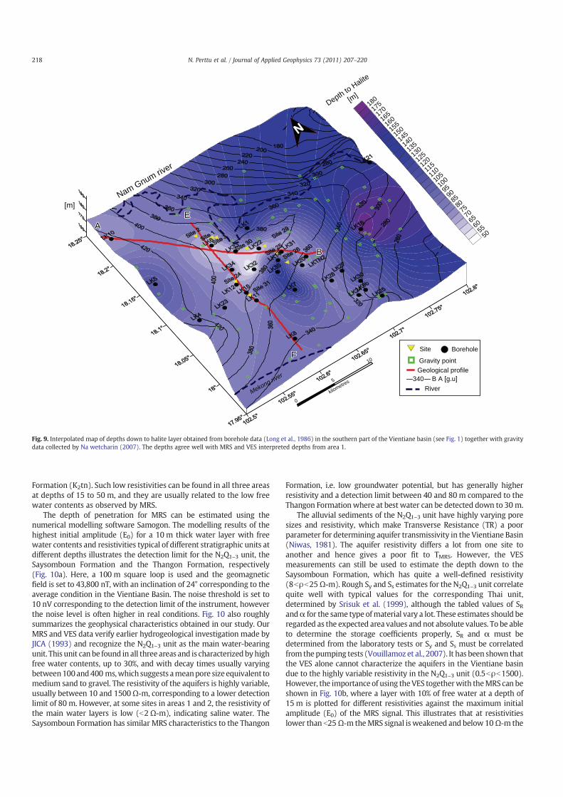
Formation (K2tn). Such low resistivities can be found in all three areasat depths of 15 to 50 m, and they are usually related to the low freewater contents as observed by MRS.
The depth of penetration for MRS can be estimated using thenumerical modelling software Samogon. The modelling results of thehighest initial amplitude (E0) for a 10 m thick water layer with freewater contents and resistivities typical of different stratigraphic units atdifferent depths illustrates the detection limit for the N2Q1–3 unit, theSaysomboun Formation and the Thangon Formation, respectively(Fig. 10a). Here, a 100 m square loop is used and the geomagneticfield is set to 43,800 nT, with an inclination of 24° corresponding to theaverage condition in the Vientiane Basin. The noise threshold is set to10 nV corresponding to the detection limit of the instrument, howeverthe noise level is often higher in real conditions. Fig. 10 also roughlysummarizes the geophysical characteristics obtained in our study. OurMRS and VES data verify earlier hydrogeological investigation made byJICA (1993) and recognize the N2Q1–3 unit as the main water-bearingunit. This unit canbe found in all three areas and is characterized byhighfree water contents, up to 30%, and with decay times usually varyingbetween100and400 ms,which suggests ameanpore size equivalent tomedium sand to gravel. The resistivity of the aquifers is highly variable,usually between 10 and 1500Ω-m, corresponding to a lower detectionlimit of 80 m. However, at some sites in areas 1 and 2, the resistivity ofthe main water layers is low (b2 Ω-m), indicating saline water. TheSaysomboun Formation has similar MRS characteristics to the Thangon
Formation, i.e. low groundwater potential, but has generally higherresistivity and a detection limit between 40 and 80 m compared to theThangon Formationwhere at best water can be detected down to 30 m.
The alluvial sediments of the N2Q1–3 unit have highly varying poresizes and resistivity, which make Transverse Resistance (TR) a poorparameter for determining aquifer transmissivity in the Vientiane Basin(Niwas, 1981). The aquifer resistivity differs a lot from one site toanother and hence gives a poor fit to TMRS. However, the VESmeasurements can still be used to estimate the depth down to theSaysomboun Formation, which has quite a well-defined resistivity(8bρb25 Ω-m). Rough Sy and Ss estimates for the N2Q1–3 unit correlatequite well with typical values for the corresponding Thai unit,determined by Srisuk et al. (1999), although the tabled values of SRandα for the same type ofmaterial vary a lot. These estimates should beregarded as the expected area values and not absolute values. To be ableto determine the storage coefficients properly, SR and α must bedetermined from the laboratory tests or Sy and Ss must be correlatedfrom thepumping tests (Vouillamoz et al., 2007). It has been shown thatthe VES alone cannot characterize the aquifers in the Vientiane basindue to the highly variable resistivity in the N2Q1–3 unit (0.5bρb1500).However, the importance of using theVES togetherwith theMRS can beshown in Fig. 10b, where a layer with 10% of free water at a depth of15 m is plotted for different resistivities against the maximum initialamplitude (E0) of the MRS signal. This illustrates that at resistivitieslower than b25 Ω-m theMRS signal is weakened and below 10 Ω-m the
5055606570758085909510010
5110115120125130135140145150155160165170175180Depth to Halite
[m]
F
EA
B
F
EA
B
0
5
10
kilometres
Site
Geological profile
[m]
340 B A [g.u]
Nam Gnum river
Borehole
Gravity point
River
N
Mekong river
Fig. 9. Interpolated map of depths down to halite layer obtained from borehole data (Long et al., 1986) in the southern part of the Vientiane basin (see Fig. 1) together with gravitydata collected by Na wetcharin (2007). The depths agree well with MRS and VES interpreted depths from area 1.
218 N. Perttu et al. / Journal of Applied Geophysics 73 (2011) 207–220
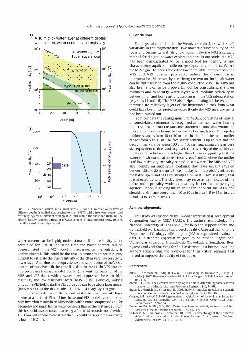
water content can be highly underestimated if the resistivity is notaccounted for. But at the same time the water content can beoverestimated if the VES model is inaccurate, i.e. the resistivity isunderestimated. This could be the case in some sites since it is verydifficult to estimate the true resistivity of the often very low resistivitylower layer. Also, due to the equivalence and suppression of the VES, anumber ofmodels can fit the samefield data. At site 11, the VES data areinterpreted as afive layermodel (Fig. 3c) (in a joint interpretation of theMRS and VES data), with a water layer suppressed between highresistivity and low resistivity layers (RMS=5.1%). However, lookingonly at the VES field data, the VES curve appears to be a four layermodel(RMS=5.3%). In the first model, the low resistivity layer begins at adepth of 22 m, whereas in the second model the low resistivity layerbegins at a depth of 15 m. Using the second VES model as input to theMRS inversion results in anMRSmodelwith amore compressed aquifergeometry andmuch higherwater contents than in thefirstmodel. Fromthis it should also be noted that using a first MRS smooth model with a100 Ω-m half sphere to constrain the VES could be risky if the resistivityis low (b10Ω-m).
6. Conclusions
The physical conditions in the Vientiane basin, Laos, with smallvariations in the magnetic field, low magnetic susceptibility of therocks and sediments and fairly low noise, make the MRS a suitablemethod for the groundwater exploration here. In our study, the MRShas been demonstrated to be a good tool for identifying andcharacterizing aquifers in different geological environments. Wherethe MRS signal-to-noise ratio is too low for reliable interpretation, theMRS and VES together proves to reduce the uncertainty ininterpretation. Moreover, by combining the two methods, salt watercan be distinguished from the highly conductive clay. The MRS hasalso been shown to be a powerful tool for constraining the layerthickness and to identify water layers with medium resistivity inbetween high and low resistivity structures in the VES interpretation(e.g. sites 11 and 16). The MRS also helps to distinguish between theintermediate resistivity layers of the impermeable rock from whatcould have been interpreted as water if only the VES measurementshad been carried out.
From our data the stratigraphic unit N2Q1–3, consisting of alluvialunconsolidated sediments, is recognized as the main water bearingunit. The results from the MRS measurements show that within theregion there is usually one to two water bearing layers. The aquiferthickness ranges from 10 to 40 m and the depth of the main aquiferranges from 5 to 15 m. The free water content is up to 30% and thedecay times vary between 100 and 400 ms, suggesting a mean poresize equivalent to fine sand to gravel. The resistivity of the aquifers ishighly variable but is usually higher than 10 Ω-m suggesting that thewater is fresh, except at some sites in areas 1 and 2, where the aquiferis of low resistivity, probably related to salt water. The MRS and VESalso identify an underlying confining clay layer usually situatedbetween 25 and 50 m depth. Since this clay is most probably related tothe halite layers and has a resistivity as low as 0.5 Ω-m, it is likely thatit is affected by salt. The clay layer may serve as an indicator of thehalite and it probably works as a salinity barrier for the overlyingaquifers. Hence, in guiding future drilling in the Vientiane Basin, oneshould not drill any deeper than 10 to 60 m in area 1, 5 to 15 m in area2 and 10 to 30 m in area 3.
Acknowledgements
This study was funded by the Swedish International DevelopmentCooperation Agency (SIDA-SAREC). The authors acknowledge theNational University of Laos (NUoL) for help and support before andduring field work, making this project a reality. A special thanks to theDepartment of Geology andMining and JICA, who provided invaluabledata. Our deepest appreciation goes to Sounthone Singsoupho,Viengthong Xayavong, Titusadewale Olowokudejo, Sengthong Bou-nyavongand and Xou Yang for field assistance. Last but not least, theauthors acknowledge the reviewers for their critical remarks thathelped to improve the quality of this paper.
References
Allen, D., Andreani, M., Badry, R., Flaum, C., Gossenberg, P., Horkowitz, J., Singer, J.,White, J., 1997. How to use borehole NMR. Schlumberger's Oilfield Review summer,pp. 34–57.
Archie, G.E., 1942. The electrical resistivity log as an aid in determining some reservoircharacteristics. Metallurgical and Petroleum Engineers 146, 54–62.
Braun, M., Hertrich, M., Yaramanci, U., 2005. Study on complex inversion of magneticresonance sounding signals. Near Surface Geophysics 3 (3), 155–163.
Cooper, H.H., Jacob, C.E., 1946. A generalized graphical method for evaluating formationconstants and summarizing well field history. American Geophysical UnionTransactions 27, 526–534.
Domenico, P.A., Mifflin, M.D., 1965. Water from low-permeability sediments and landsubsidence. Water Resources Research 1 (4), 563–576.
El Tabakh, M., Utha-Aroon, C., Schreiber, B.C., 1999. Sedimentology of the CretaceousMaha Sarakham evaporites in the Khorat Plateau of northeastern Thailand.Sedimentary Geology 123 (1–2), 31–62.
0 20 40 60 80 100100
101
102
103
100
101
102
103
Depth [m]
N2Q1-3, T2*=150 ms
K2sb, T2*=70 ms
K2tn, T2*=40 ms
Instrument limitation
B0=43800nT, I=24˚,100 m square loop
A 10 m thick water layer at different depthswith different water contents and resistivity
40
20
0
[m]
10
30
50
104 103 102 101 100 10-1
80
120
160
200
-6
-4
-2
0
ρ [ohm-m]
Max
imum
E0
[nV
]M
axim
um E
0 [n
V]
Max
imum
E0
[nV
]U
nder
estim
atio
n of
θM
RS [%
]
a)
b)
10%
Fig. 10. a) Modelled highest initial amplitudes (E0) for a 10 m thick water layer atdifferent depths (modified after Legchenko et al. (1997)) with a free water content andresistivity typical of different stratigraphic units within the Vientiane Basin. b) Theeffect of resistivity on the estimation of water content [%] illustrates that below 10 Ω-m,the MRS signal is severely affected.
219N. Perttu et al. / Journal of Applied Geophysics 73 (2011) 207–220
Guillen, A., Legchenko, A., 2002a. Application of linear programming techniques to theinversion of proton magnetic resonance measurements for water prospecting fromthe surface. Journal of Applied Geophysics 50 (1–2), 149–162.
Guillen, A., Legchenko, A., 2002b. Inversion of surface nuclear magnetic resonance databy an adapted Monte Carlo method applied to water resource characterization.Journal of Applied Geophysics 50 (1–2), 193–205.
Hamill, L., Bell, F.G., 1986. Groundwater Resource Development. Buttersworth, London.344 pp.
JICA, 1993. Design Study Report on the Project for Groundwater Development inVientiane Province in Lao People's Democratic Republic. Japan InternationalCooperation Agency (JICA). 94 pp.
JICA, 1994. Drilling Logs from the Groundwater Development in the Vientiane ProvinceProject. Japan International Cooperation Agency (JICA), JICA local office in PhonHong, Vientiane Province, Laos, p. 718.
JICA, 2000. Japan International Cooperation Agency. The study on Rural WaterSupply and Sanitation Improvement in the Northwest Region in the LaoPeople's Democratic Republic, Progress Report 2. Japan International Cooper-ation Agency (JICA), Ministry of health, National Center for EnvironmentalHealth and Water Supply. 14 pp.
Johnson, A.I., 1967. Specific yield; compilation of specific yields for various materials.U.S. Geological Survey Professional Paper: D1–D74.
Kirsch, R., 2006. Groundwater Geophysics: A Tool for Hydrogeology. Springer-Verlag,Berlin Heidelberg. 493 pp.
Legchenko, A., 2004. Magnetic resonance sounding: enhanced modeling of a phaseshift. Applied Magnetic Resonance 25 (3–4), 621–636.
Legchenko, A., 2005. Improved modelling of the magnetic resonance signal in thepresence of shallow aquifers. Near Surface Geophysics 3 (3), 121–130.
Legchenko, A., 2006. MRS measurements and inversion in presence of EM noise. 3rdMagnetic Resonance Sounding International Workshop. MRS 2006 Proceedings,Spain, Madrid, pp. 21–24.
Legchenko, A., 2008. Interpretation of magnetic resonance soundings in rocks with highelectrical conductivity. Journal of Applied Geophysics 66 (3–4), 118–127.
Legchenko, A.V., Shushakov, O.A., 1998. Inversion of surface NMR data. Geophysics 63(1), 75–84.
Legchenko, A., Valla, P., 2002. A review of the basic principles for proton magneticresonance sounding measurements. Journal of Applied Geophysics 50 (1–2),3–19.
Legchenko, A., Valla, P., 2003. Removal of power-line harmonics from proton magneticresonance measurements. Journal of Applied Geophysics 53 (2–3), 103–120.
Legchenko, A.V., Beauce, A., Guillen, A., Valla, P., Bernard, J., 1997. Naturalvariations in the magnetic resonance signal used in PMR groundwaterprospecting from the surface. Journal of Environmental and EngineeringGeophysics 2, 173–190.
Legchenko, A., et al., 2004. Magnetic resonance sounding applied to aquifercharacterization. Ground Water 42 (3), 363–373.
Long, N.X., Lam, N.X., Canh, N.D., 1986. Report on Geological Data for Potassium andManganese in Thangon Region, Dong Bang, Vientiane, 1986. Department ofGeology and Mining, Vientiane, Laos, Vientiane.
Lovatt Smith, P.F., Stokes, R.B., Bristow, C., Carter, A., 1996. Mid-Cretaceous inversion inthe northern Khorat Plateau of Lao PDR and Thailand. Tectonic evolution ofSoutheast Asia. Geological Society Special Publication 233–247 (No. 106).
Lubczynski, M., Roy, J., 2003. Hydrogeological interpretation and potential of the newmagnetic resonance sounding (MRS) method. Journal of Hydrology 283 (1–4),19–40.
Maillet, R., 1947. The fundamental equations of electrical prospecting. Geophysics12 (4), 529–556.
Medlicott, K., 2001. Water, Sanitation and Environmental Health in Rural Laos PDR. KAPStudy for UNICEF, WES Section. 20 pp.
Mohnke, O., Yaramanci, U., 2002. Smooth and block inversion of surface NMRamplitudes and decay times using simulated annealing. Journal of AppliedGeophysics 50 (1–2), 163–177.
Morris, D.A., Johnson, A.I., 1967. Summary of hydrologic and physical properties of rockand soil materials, as analyzed by the hydrologic laboratory of the U. S. GeologicalSurvey, 1948–60. U.S. Geological Survey Water-Supply Paper: D1–D42.
Na wetcharin, S., 2007. Gravity Anomalies in Vientiane Capital, Lao PDR. Prince ofSongkla University, Hatyai, Thailand. 85 pp.
Niwas, S., 1981. Estimation of aquifer transmissivity from Dar-Zarrouk parameters inporous media. Journal of Hydrology 50 (1–4), 393–399.
Parasnis, D.S., 1997. Principles of Applied Geophysics. Chapman & Hall. 429 pp.Ponzini, G., 1984. Empirical relation between electrical transverse resistance and
hydraulic transmissivity. Geoexploration 22 (1), 1–15.Salem, H., 1999. Determination of fluid transmissivity and electric transverse resistance
for shallow aquifers and deep reservoirs from surface and well-log electricmeasurements. Hydrology and Earth System Sciences 3 (3), 421–427.
Shirov, M., Legchenko, A., Creer, G., 1991. A new direct non-invasive groundwaterdetection technology for Australia. Exploration Geophysics 22, 333–338.
Srisuk, K., Sriboonlue, V., Buaphan, C., 1999. Groundwater flow, saline water andsaline soils in the Central Khorat Basin, northeast Thailand. Symposium onMineral, Energy and Water Resources of Thailand: Towards the Year 2000,Thailand, pp. 238–251.
STEA, 2001. State of the Environment Report. 2001: Lao People's Democratic Republic.UNEP, RRC.AP, p. 82.
Stuart-Fox, M., Rooney, D.F., 2006. Laos, Land and Resources and EnvironmentalConcerns. Encarta (electronic resource).
Sundberg, K., 1932. Effect of impregnating waters on conductivity of soils and rocks.AIME 97, 367–391.
Theis, C.V., 1935. The relation between the lowering of the piezometric surface and rateand duration of discharge of a well using groundwater storage: AmericanGeophysical Union. Transactions — Institution of Mining and Metallurgy. SectionA. Mining Industry 2, 519.
Velpen, V., 1988. Resist87: A computer processing software for DC resistivityinterpretation, ITC-Delft, The Netherlands, pp. M.sc. thesis.
Vouillamoz, J.M., Descloitres, M., Bernard, J., Fourcassier, P., Romagny, L., 2002.Application of integrated magnetic resonance sounding and resistivity methodsfor borehole implementation. A case study in Cambodia. Journal of AppliedGeophysics 50 (1–2), 67–81.
Vouillamoz, J.M., Chatenoux, B., Mathieu, F., Baltassat, J.M., Legchenko, A., 2007.Efficiency of joint use of MRS and VES to characterize coastal aquifer in Myanmar.Journal of Applied Geophysics 61 (2), 142–154.
Wannakomol, A., 2005. Soil and groundwater salinization problems in the KhoratPlateau, NE Thailand, Integrated Study of Remote Sensing, Geophysical and FieldData. PhD Thesis, Freie Universität Berlin, 204 pp.
Williamson, D.R., Peck, A.J., Turner, J.V., Arunin, S., 1989. Groundwater hydrology andsalinity in a valley in Northeast Thailand. Groundwater Contamination IAHS-AISHPublication 185, 147–154.
Worthington, P., 1993. The uses and abuses of the Archie equations; 1, The formationfactor–porosity relationship. Journal of Applied Geophysics 30 (3), 215–228.
Xayavong, V., Lohawijarn, W., Bhongsuwan, T., 2008. Application of Gravity andResistivity for Mappiong Regional Structures of Vientiane Basin, Lao PDR. Prince ofSongkla University, HatYai. 17 pp.
Yaramanci, U., 2004. New technologies in ground water exploration; surface nuclearmagnetic resonance. Geologica Acta 2, 109–120.
220 N. Perttu et al. / Journal of Applied Geophysics 73 (2011) 207–220
Paper II
Determining Water Quality Parameters of Aquifers in the Vientiane Basin, Laos, Using Geophysical and Water Chemistry Data.
Perttu, N., Wattanasen, K., Phommasone, S-Å., Elming (2011) Near Surface Geophysics, 9: 381-395

© 2011 European Association of Geoscientists & Engineers 381
Determining water quality parameters of aquifers in the Vientiane Basin, Laos, using geophysical and water chemistry data
Nils Perttu1*, Kamhaeng Wattanasen2, Khamphouth Phommasone3 and
Sten-Åke Elming1
1 Division of Ore Geology and Applied Geophysics, Luleå University of Technology, 971 87 Luleå, Sweden2 Department of Physics, Faculty of Science, Prince of Songkla University, HatYa 90112, Thailand3 Department of Physics, National University of Laos, PO Box 7322, DongDok Campus, Vientiane, Laos
Received December 2009, revision accepted April 2011
ABSTRACTThe aim of this study is to test the possibility of using magnetic resonance sounding (MRS) and
vertical electrical sounding (VES) together with groundwater chemistry data from shallow and deep
wells to distinguish freshwater aquifers from salt affected groundwater and moreover determine
water quality parameters directly from geophysical data. Three study areas within the Vientiane
Basin, including 46 sites and 38 sampled wells, have been chosen for the study. The main water qual-
ity parameters affecting the water conductivity in the Vientiane Basin are total dissolved solids (TDS)
and hardness and to a minor extent chloride, which all have shown to have fairly high correlation to
the electrical conductivity (EC) of groundwater. The resistivity of the aquifers is highly variable but
is most often above 4 m, suggesting fresh water. No wells in the investigated areas have water qual-
ity parameters exceeding the limit for unacceptable drinking or irrigation water. There is a fairly
strong relationship between the conductivity of water from deep wells and the conductivity of the
main water bearing layer determined by VES, where the best fit is obtained using:
EC[μS/cm] = 0.4694VES[μS/cm], R2 = 0.69. However, due to equivalence in the VES interpretation
and the difficulty to estimate the resistivity contribution from finer sediments, the equation may be
seen and used as guidance to good water quality only within the Vientiane Basin area or in other areas
with similar geology. The MRS results have been used to identify water layers in the VES inversion
results to decrease the uncertainty in the interpretation The combination of MRS and VES techniques
has been successful in distinguishing high conductive clay and mudstone from water bearing layers
and moreover freshwater aquifers from salt affected water. Altogether, this makes MRS and VES very
promising tools for guidance of future drilling and water quality estimation.
trations of domestic waste and excreta from farm animals,
have lead to a high morbidity rate (JICA 1993; Medlicott
2001). In 1993, the ‘Project for Groundwater Development in
Vientiane Province’ was implemented by the Japan
International Cooperation Agency (JICA), aiming at raising
the water supply ratio in the rural areas by drilling deep wells
(JICA 1993). In total 118 deep wells were drilled and when
evaluating the project in 2000, as much as 60% of the wells
were not used for drinking due to bad water quality or main-
tenance problems (JICA 2000). The bad water quality was
partially due to salt in the groundwater. Rock salt naturally
occurs within the basin as shallow as 50 m in the Thangon
Formation (Williamson et al. 1989; JICA 1993; Srisuk et al. 1999; Wannakomol 2005).
INTRODUCTIONWhen evaluating aquifers for drinking water usage, the qual-
ity of groundwater is as important as its quantity. In Lao
People’s Democratic Republic (Laos), located in the middle
of Southeast Asia (Fig. 1), only 60% of the urban and 51% of
the rural population had direct access to water supply in 1998
(STEA 2001). Most Lao people live in rural parts and are
heavily dependent on dug wells as their main water source.
However, deep wells, river water and rainwater are also used
(Medlicott 2001). Dug wells usually dry out during the dry
period and in addition, water-borne diseases caused by infil-
Near Surface Geophysics, 2011, 9, 381-395 doi:10.3997/1873-0604.2011014
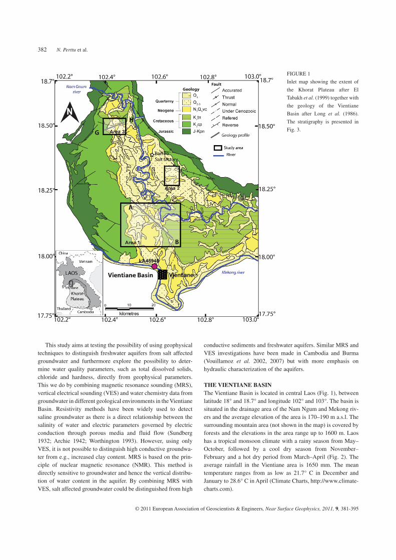
N. Perttu et al.382
© 2011 European Association of Geoscientists & Engineers, Near Surface Geophysics, 2011, 9, 381-395
conductive sediments and freshwater aquifers. Similar MRS and
VES investigations have been made in Cambodia and Burma
(Vouillamoz et al. 2002, 2007) but with more emphasis on
hydraulic characterization of the aquifers.
THE VIENTIANE BASINThe Vientiane Basin is located in central Laos (Fig. 1), between
latitude 18° and 18.7° and longitude 102° and 103°. The basin is
situated in the drainage area of the Nam Ngum and Mekong riv-
ers and the average elevation of the area is 170–190 m a.s.l. The
surrounding mountain area (not shown in the map) is covered by
forests and the elevations in the area range up to 1600 m. Laos
has a tropical monsoon climate with a rainy season from May–
October, followed by a cool dry season from November–
February and a hot dry period from March–April (Fig. 2). The
average rainfall in the Vientiane area is 1650 mm. The mean
temperature ranges from as low as 21.7° C in December and
January to 28.6° C in April (Climate Charts, http://www.climate-
charts.com).
This study aims at testing the possibility of using geophysical
techniques to distinguish freshwater aquifers from salt affected
groundwater and furthermore explore the possibility to deter-
mine water quality parameters, such as total dissolved solids,
chloride and hardness, directly from geophysical parameters.
This we do by combining magnetic resonance sounding (MRS),
vertical electrical sounding (VES) and water chemistry data from
groundwater in different geological environments in the Vientiane
Basin. Resistivity methods have been widely used to detect
saline groundwater as there is a direct relationship between the
salinity of water and electric parameters governed by electric
conduction through porous media and fluid flow (Sundberg
1932; Archie 1942; Worthington 1993). However, using only
VES, it is not possible to distinguish high conductive groundwa-
ter from e.g., increased clay content. MRS is based on the prin-
ciple of nuclear magnetic resonance (NMR). This method is
directly sensitive to groundwater and hence the vertical distribu-
tion of water content in the aquifer. By combining MRS with
VES, salt affected groundwater could be distinguished from high
FIGURE 1
Inlet map showing the extent of
the Khorat Plateau after El
Tabakh et al. (1999) together with
the geology of the Vientiane
Basin after Long et al. (1986).
The stratigraphy is presented in
Fig. 3.
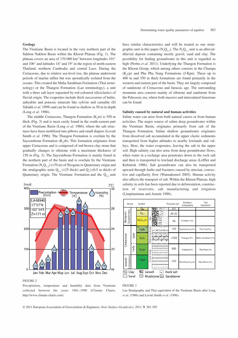
Determining water quality parameters of aquifers 383
© 2011 European Association of Geoscientists & Engineers, Near Surface Geophysics, 2011, 9, 381-395
have similar characteristics and will be treated as one strati-
graphic unit in this paper (N2Q
1-3). The N
2Q
1-3 unit is an alluvial-
diluvial deposit containing mostly gravel, sand and clay. The
possibility for finding groundwater in this unit is regarded as
high (Perttu et al. 2011). Underlying the Thangon Formation is
the Khorat Group, which among others consists in the Champa
(K2cp) and Phu Pha Nang Formations (J-Kpn). These up to
400 m and 350 m thick formations are found primarily in the
western and eastern part of the basin. They are largely composed
of sandstone of Cretaceous and Jurassic age. The surrounding
mountain area consists mainly of siltstone and sandstone from
the Paleozoic era, where both massive and intercalated limestone
can be found.
Salinity caused by natural and human activitiesSaline water can arise from both natural causes or from human
activities. The major source of saline deep groundwater within
the Vientiane Basin, originates primarily from salt of the
Thangon Formation. Saline shallow groundwater originates
from dissolved salt accumulated in the upper clastic sediments
transported from higher altitudes to nearby lowlands and val-
leys. Here, the water evaporates, leaving the salt in the upper
soil. High salinity can also arise from deep groundwater flows,
when water in a recharge area penetrates down to the rock salt
and then is transported to lowland discharge areas (Löffler and
Kubiniok 1986). Salt groundwater can also be transported
upward through faults and fractures caused by artesian, convec-
tive and capillarity flow (Wannakomol 2005). Human activity
also affects the transport of salt. Within the Khorat Plateau, high
salinity in soils has been reported due to deforestation, construc-
tion of reservoirs, salt manufacturing and irrigation
(Limpinuntana and Arunin 1986).
GeologyThe Vientiane Basin is located in the very northern part of the
Sakhon Nakhon Basin within the Khorat Plateau (Fig. 1). The
plateau covers an area of 170 000 km2 between longitudes 101°
and 106° and latitudes 14° and 19° in the region of north-eastern
Thailand, northern Cambodia and central Laos. During the
Cretaceous, due to relative sea-level rise, the plateau underwent
periods of marine influx but was sporadically isolated from the
oceans. This created the Maha Sarakham Formation (Thai termi-
nology) or the Thangon Formation (Lao terminology), a unit
with a three salt layer separated by red-coloured siliciclastics of
fluvial origin. The evaporites include thick successions of halite,
anhydrite and potassic minerals like sylivite and carnalite (El
Tabakh et al. 1999) and can be found as shallow as 50 m in depth
(Long et al. 1986).
The middle Cretaceous, Thangon Formation (K2tn) is 550 m
thick (Fig. 3) and is most easily found in the south-eastern part
of the Vientiane Basin (Long et al. 1986), where the salt struc-
tures have been mobilized into pillows and small diapers (Lovatt
Smith et al. 1996). The Thangon Formation is overlain by the
Saysomboun Formation (K2sb). This formation originates from
upper Cretaceous and is composed of red-brown clay-stone that
gradually changes to siltstone with a maximum thickness of
150 m (Fig. 3). The Saysomboun Formation is mainly found in
the northern part of the basin and is overlain by the Vientiane
Formation (N2Q
1-2) (<70 m) of Neogene to Quaternary origin and
the stratigraphic units Q2-3
(<25 thick) and Q4 (<0.5 m thick) of
Quaternary origin. The Vientiane Formation and the Q
2-3 unit
FIGURE 2
Precipitation, temperature and humidity data from Vientiane
collected between the years 1961–1990 (Climate Charts,
http://www.climate-charts.com).
FIGURE 3
Lao Stratigraphy and Thai equivalent of the Vientiane Basin after Long
et al. (1986) and Lovatt Smith et al. (1996).
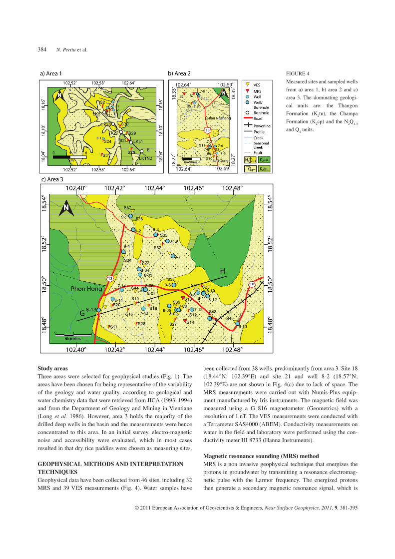
N. Perttu et al.384
© 2011 European Association of Geoscientists & Engineers, Near Surface Geophysics, 2011, 9, 381-395
been collected from 38 wells, predominantly from area 3. Site 18
(18.44°N; 102.39°E) and site 21 and well 8-2 (18.57°N;
102.39°E) are not shown in Fig. 4(c) due to lack of space. The
MRS measurements were carried out with Numis-Plus equip-
ment manufactured by Iris instruments. The magnetic field was
measured using a G 816 magnetometer (Geometrics) with a
resolution of 1 nT. The VES measurements were conducted with
a Terrameter SAS4000 (ABEM). Conductivity measurements on
water in the field and laboratory were performed using the con-
ductivity meter HI 8733 (Hanna Instruments).
Magnetic resonance sounding (MRS) methodMRS is a non invasive geophysical technique that energizes the
protons in groundwater by transmitting a resonance electromag-
netic pulse with the Larmor frequency. The energized protons
then generate a secondary magnetic resonance signal, which is
Study areasThree areas were selected for geophysical studies (Fig. 1). The
areas have been chosen for being representative of the variability
of the geology and water quality, according to geological and
water chemistry data that were retrieved from JICA (1993, 1994)
and from the Department of Geology and Mining in Vientiane
(Long et al. 1986). However, area 3 holds the majority of the
drilled deep wells in the basin and the measurements were hence
concentrated to this area. In an initial survey, electro-magnetic
noise and accessibility were evaluated, which in most cases
resulted in that dry rice paddies were chosen as measuring sites.
GEOPHYSICAL METHODS AND INTERPRETATION TECHNIQUESGeophysical data have been collected from 46 sites, including 32
MRS and 39 VES measurements (Fig. 4). Water samples have
FIGURE 4
Measured sites and sampled wells
from a) area 1, b) area 2 and c)
area 3. The dominating geologi-
cal units are: the Thangon
Formation (K2tn), the Champa
Formation (K2cp) and the N
2Q
1-3
and Q4 units.
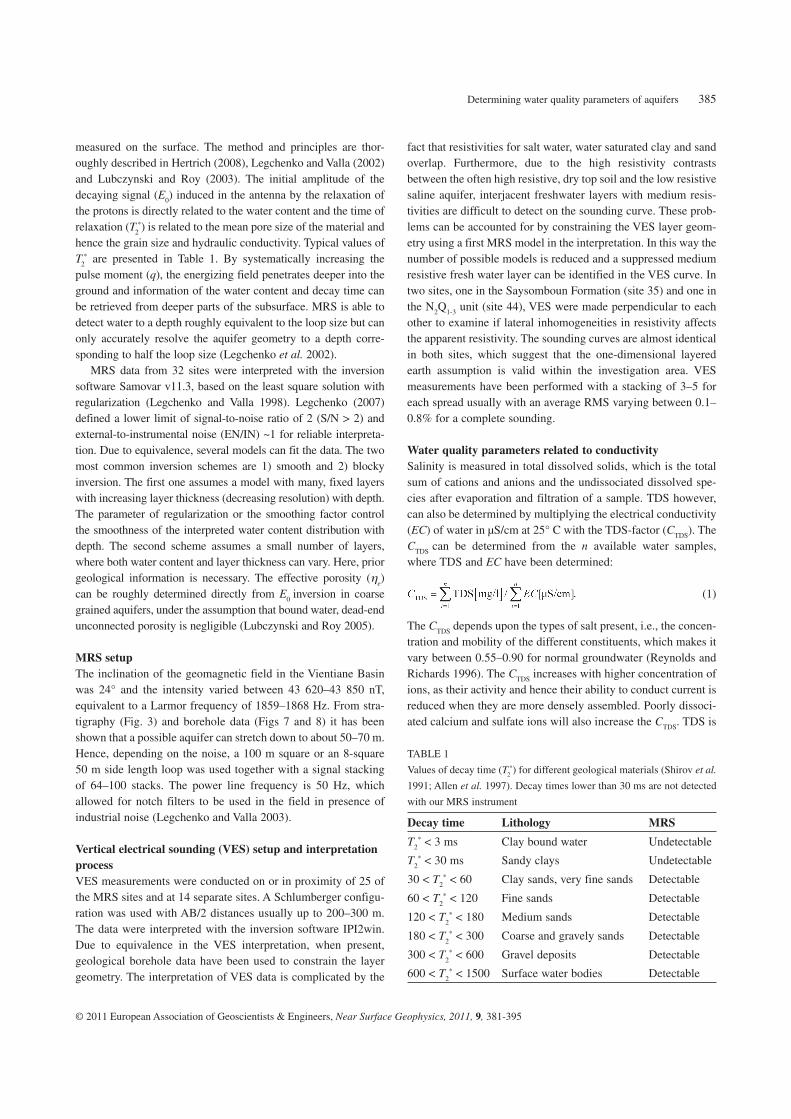
Determining water quality parameters of aquifers 385
© 2011 European Association of Geoscientists & Engineers, Near Surface Geophysics, 2011, 9, 381-395
fact that resistivities for salt water, water saturated clay and sand
overlap. Furthermore, due to the high resistivity contrasts
between the often high resistive, dry top soil and the low resistive
saline aquifer, interjacent freshwater layers with medium resis-
tivities are difficult to detect on the sounding curve. These prob-
lems can be accounted for by constraining the VES layer geom-
etry using a first MRS model in the interpretation. In this way the
number of possible models is reduced and a suppressed medium
resistive fresh water layer can be identified in the VES curve. In
two sites, one in the Saysomboun Formation (site 35) and one in
the N2Q
1-3 unit (site 44), VES were made perpendicular to each
other to examine if lateral inhomogeneities in resistivity affects
the apparent resistivity. The sounding curves are almost identical
in both sites, which suggest that the one-dimensional layered
earth assumption is valid within the investigation area. VES
measurements have been performed with a stacking of 3–5 for
each spread usually with an average RMS varying between 0.1–
0.8% for a complete sounding.
Water quality parameters related to conductivitySalinity is measured in total dissolved solids, which is the total
sum of cations and anions and the undissociated dissolved spe-
cies after evaporation and filtration of a sample. TDS however,
can also be determined by multiplying the electrical conductivity
(EC) of water in μS/cm at 25° C with the TDS-factor (CTDS
). The
CTDS can be determined from the n available water samples,
where TDS and EC have been determined:
(1)
The CTDS
depends upon the types of salt present, i.e., the concen-
tration and mobility of the different constituents, which makes it
vary between 0.55–0.90 for normal groundwater (Reynolds and
Richards 1996). The CTDS
increases with higher concentration of
ions, as their activity and hence their ability to conduct current is
reduced when they are more densely assembled. Poorly dissoci-
ated calcium and sulfate ions will also increase the CTDS
. TDS is
measured on the surface. The method and principles are thor-
oughly described in Hertrich (2008), Legchenko and Valla (2002)
and Lubczynski and Roy (2003). The initial amplitude of the
decaying signal (E0) induced in the antenna by the relaxation of
the protons is directly related to the water content and the time of
relaxation (T2*) is related to the mean pore size of the material and
hence the grain size and hydraulic conductivity. Typical values of
T2* are presented in Table 1. By systematically increasing the
pulse moment (q), the energizing field penetrates deeper into the
ground and information of the water content and decay time can
be retrieved from deeper parts of the subsurface. MRS is able to
detect water to a depth roughly equivalent to the loop size but can
only accurately resolve the aquifer geometry to a depth corre-
sponding to half the loop size (Legchenko et al. 2002).
MRS data from 32 sites were interpreted with the inversion
software Samovar v11.3, based on the least square solution with
regularization (Legchenko and Valla 1998). Legchenko (2007)
defined a lower limit of signal-to-noise ratio of 2 (S/N > 2) and
external-to-instrumental noise (EN/IN) ~1 for reliable interpreta-
tion. Due to equivalence, several models can fit the data. The two
most common inversion schemes are 1) smooth and 2) blocky
inversion. The first one assumes a model with many, fixed layers
with increasing layer thickness (decreasing resolution) with depth.
The parameter of regularization or the smoothing factor control
the smoothness of the interpreted water content distribution with
depth. The second scheme assumes a small number of layers,
where both water content and layer thickness can vary. Here, prior
geological information is necessary. The effective porosity (e)
can be roughly determined directly from E0
inversion in coarse
grained aquifers, under the assumption that bound water, dead-end
unconnected porosity is negligible (Lubczynski and Roy 2005).
MRS setupThe inclination of the geomagnetic field in the Vientiane Basin
was 24° and the intensity varied between 43 620–43 850 nT,
equivalent to a Larmor frequency of 1859–1868 Hz. From stra-
tigraphy (Fig. 3) and borehole data (Figs 7 and 8) it has been
shown that a possible aquifer can stretch down to about 50–70 m.
Hence, depending on the noise, a 100 m square or an 8-square
50 m side length loop was used together with a signal stacking
of 64–100 stacks. The power line frequency is 50 Hz, which
allowed for notch filters to be used in the field in presence of
industrial noise (Legchenko and Valla 2003).
Vertical electrical sounding (VES) setup and interpretation processVES measurements were conducted on or in proximity of 25 of
the MRS sites and at 14 separate sites. A Schlumberger configu-
ration was used with AB/2 distances usually up to 200–300 m.
The data were interpreted with the inversion software IPI2win.
Due to equivalence in the VES interpretation, when present,
geological borehole data have been used to constrain the layer
geometry. The interpretation of VES data is complicated by the
TABLE 1
Values of decay time (T2*) for different geological materials (Shirov et al.
1991; Allen et al. 1997). Decay times lower than 30 ms are not detected
with our MRS instrument
Decay time Lithology MRS
T2* < 3 ms Clay bound water Undetectable
T2* < 30 ms Sandy clays Undetectable
30 < T2* < 60 Clay sands, very fine sands Detectable
60 < T2* < 120 Fine sands Detectable
120 < T2* < 180 Medium sands Detectable
180 < T2* < 300 Coarse and gravely sands Detectable
300 < T2* < 600 Gravel deposits Detectable
600 < T2* < 1500 Surface water bodies Detectable
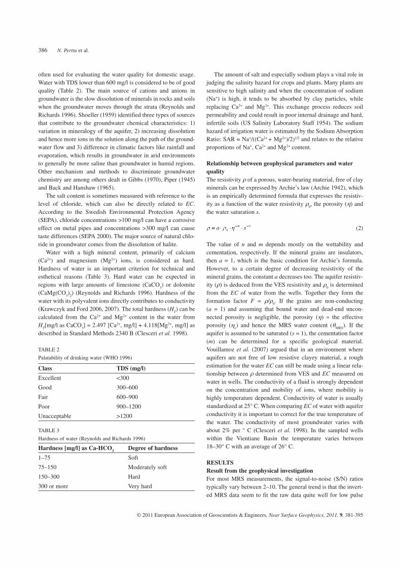
N. Perttu et al.386
© 2011 European Association of Geoscientists & Engineers, Near Surface Geophysics, 2011, 9, 381-395
The amount of salt and especially sodium plays a vital role in
judging the salinity hazard for crops and plants. Many plants are
sensitive to high salinity and when the concentration of sodium
(Na+) is high, it tends to be absorbed by clay particles, while
replacing Ca2+ and Mg2+. This exchange process reduces soil
permeability and could result in poor internal drainage and hard,
infertile soils (US Salinity Laboratory Staff 1954). The sodium
hazard of irrigation water is estimated by the Sodium Absorption
Ratio: SAR = Na+/((Ca2+ + Mg2+)/2)1/2 and relates to the relative
proportions of Na+, Ca2+ and Mg2+ content.
Relationship between geophysical parameters and water qualityThe resistivity of a porous, water-bearing material, free of clay
minerals can be expressed by Archie’s law (Archie 1942), which
is an empirically determined formula that expresses the resistiv-
ity as a function of the water resistivity 0, the porosity ( ) and
the water saturation s.
(2)
The value of n and m depends mostly on the wettability and
cementation, respectively. If the mineral grains are insulators,
then a = 1, which is the basic condition for Archie’s formula.
However, to a certain degree of decreasing resistivity of the
mine ral grains, the constant a decreases too. The aquifer resistiv-
ity ( ) is deduced from the VES resistivity and 0 is determined
from the EC of water from the wells. Together they form the
formation factor F = /0. If the grains are non-conducting
(a = 1) and assuming that bound water and dead-end uncon-
nected porosity is negligible, the porosity ( ) ≈ the effective
porosity (e) and hence the MRS water content (
MRS). If the
aquifer is assumed to be saturated (s = 1), the cementation factor
(m) can be determined for a specific geological material.
Vouillamoz et al. (2007) argued that in an environment where
aquifers are not free of low resistive clayey material, a rough
estimation for the water EC can still be made using a linear rela-
tionship between determined from VES and EC measured on
water in wells. The conductivity of a fluid is strongly dependent
on the concentration and mobility of ions, where mobility is
highly temperature dependent. Conductivity of water is usually
standardized at 25° C. When comparing EC of water with aquifer
conductivity it is important to correct for the true temperature of
the water. The conductivity of most groundwater varies with
about 2% per ° C (Clesceri et al. 1998). In the sampled wells
within the Vientiane Basin the temperature varies between
18–30° C with an average of 26° C.
RESULTSResult from the geophysical investigationFor most MRS measurements, the signal-to-noise (S/N) ratios
typically vary between 2–10. The general trend is that the invert-
ed MRS data seem to fit the raw data quite well for low pulse
often used for evaluating the water quality for domestic usage.
Water with TDS lower than 600 mg/l is considered to be of good
quality (Table 2). The main source of cations and anions in
groundwater is the slow dissolution of minerals in rocks and soils
when the groundwater moves through the strata (Reynolds and
Richards 1996). Shoeller (1959) identified three types of sources
that contribute to the groundwater chemical characteristics: 1)
variation in mineralogy of the aquifer, 2) increasing dissolution
and hence more ions in the solution along the path of the ground-
water flow and 3) difference in climatic factors like rainfall and
evaporation, which results in groundwater in arid environments
to generally be more saline than groundwater in humid regions.
Other mechanism and methods to discriminate groundwater
chemistry are among others dealt in Gibbs (1970), Piper (1945)
and Back and Hanshaw (1965).
The salt content is sometimes measured with reference to the
level of chloride, which can also be directly related to EC.
According to the Swedish Environmental Protection Agency
(SEPA), chloride concentrations >100 mg/l can have a corrosive
effect on metal pipes and concentrations >300 mg/l can cause
taste differences (SEPA 2000). The major source of natural chlo-
ride in groundwater comes from the dissolution of halite.
Water with a high mineral content, primarily of calcium
(Ca2+) and magnesium (Mg2+) ions, is considered as hard.
Hardness of water is an important criterion for technical and
esthetical reasons (Table 3). Hard water can be expected in
regions with large amounts of limestone (CaCO3) or dolomite
(CaMg(CO3)
2) (Reynolds and Richards 1996). Hardness of the
water with its polyvalent ions directly contributes to conductivity
(Krawczyk and Ford 2006, 2007). The total hardness (HT) can be
calculated from the Ca2+ and Mg2+ content in the water from
HT[mg/l as CaCO
3] = 2.497 [Ca2+, mg/l] + 4.118[Mg2+, mg/l] as
described in Standard Methods 2340 B (Clesceri et al. 1998).
TABLE 2
Palatability of drinking water (WHO 1996)
Class TDS (mg/l)
Excellent <300
Good 300–600
Fair 600–900
Poor 900–1200
Unacceptable >1200
TABLE 3
Hardness of water (Reynolds and Richards 1996)
Hardness [mg/l] as Ca-HCO3 Degree of hardness
1–75 Soft
75–150 Moderately soft
150–300 Hard
300 or more Very hard
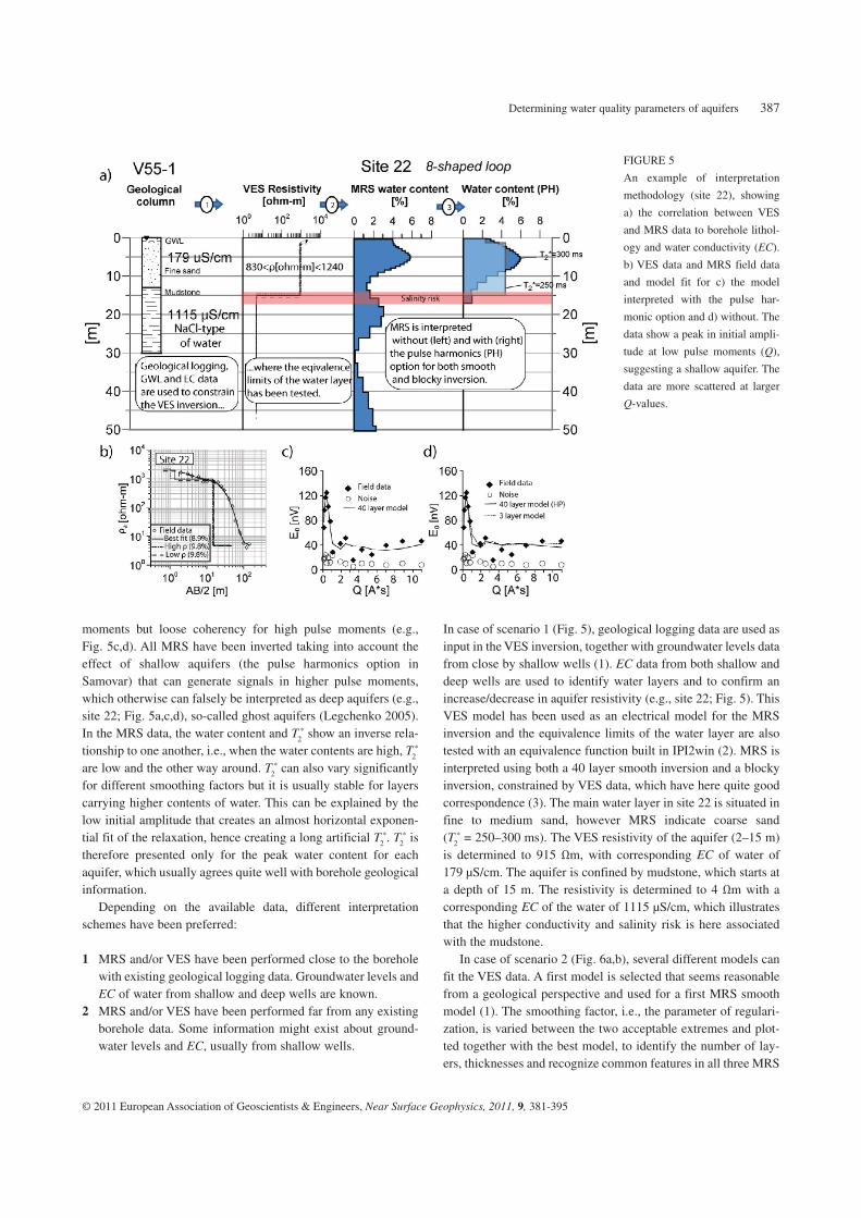
Determining water quality parameters of aquifers 387
© 2011 European Association of Geoscientists & Engineers, Near Surface Geophysics, 2011, 9, 381-395
In case of scenario 1 (Fig. 5), geological logging data are used as
input in the VES inversion, together with groundwater levels data
from close by shallow wells (1). EC data from both shallow and
deep wells are used to identify water layers and to confirm an
increase/decrease in aquifer resistivity (e.g., site 22; Fig. 5). This
VES model has been used as an electrical model for the MRS
inversion and the equivalence limits of the water layer are also
tested with an equivalence function built in IPI2win (2). MRS is
interpreted using both a 40 layer smooth inversion and a blocky
inversion, constrained by VES data, which have here quite good
correspondence (3). The main water layer in site 22 is situated in
fine to medium sand, however MRS indicate coarse sand
(T2* = 250–300 ms). The VES resistivity of the aquifer (2–15 m)
is determined to 915 Ωm, with corresponding EC of water of
179 μS/cm. The aquifer is confined by mudstone, which starts at
a depth of 15 m. The resistivity is determined to 4 Ωm with a
corresponding EC of the water of 1115 μS/cm, which illustrates
that the higher conductivity and salinity risk is here associated
with the mudstone.
In case of scenario 2 (Fig. 6a,b), several different models can
fit the VES data. A first model is selected that seems reasonable
from a geological perspective and used for a first MRS smooth
model (1). The smoothing factor, i.e., the parameter of regulari-
zation, is varied between the two acceptable extremes and plot-
ted together with the best model, to identify the number of lay-
ers, thicknesses and recognize common features in all three MRS
moments but loose coherency for high pulse moments (e.g.,
Fig. 5c,d). All MRS have been inverted taking into account the
effect of shallow aquifers (the pulse harmonics option in
Samovar) that can generate signals in higher pulse moments,
which otherwise can falsely be interpreted as deep aquifers (e.g.,
site 22; Fig. 5a,c,d), so-called ghost aquifers (Legchenko 2005).
In the MRS data, the water content and T2* show an inverse rela-
tionship to one another, i.e., when the water contents are high, T2*
are low and the other way around. T2* can also vary significantly
for different smoothing factors but it is usually stable for layers
carrying higher contents of water. This can be explained by the
low initial amplitude that creates an almost horizontal exponen-
tial fit of the relaxation, hence creating a long artificial T2*. T
2* is
therefore presented only for the peak water content for each
aquifer, which usually agrees quite well with borehole geological
information.
Depending on the available data, different interpretation
schemes have been preferred:
1 MRS and/or VES have been performed close to the borehole
with existing geological logging data. Groundwater levels and
EC of water from shallow and deep wells are known.
2 MRS and/or VES have been performed far from any existing
borehole data. Some information might exist about ground-
water levels and EC, usually from shallow wells.
FIGURE 5
An example of interpretation
methodology (site 22), showing
a) the correlation between VES
and MRS data to borehole lithol-
ogy and water conductivity (EC).
b) VES data and MRS field data
and model fit for c) the model
interpreted with the pulse har-
monic option and d) without. The
data show a peak in initial ampli-
tude at low pulse moments (Q),
suggesting a shallow aquifer. The
data are more scattered at larger
Q-values.
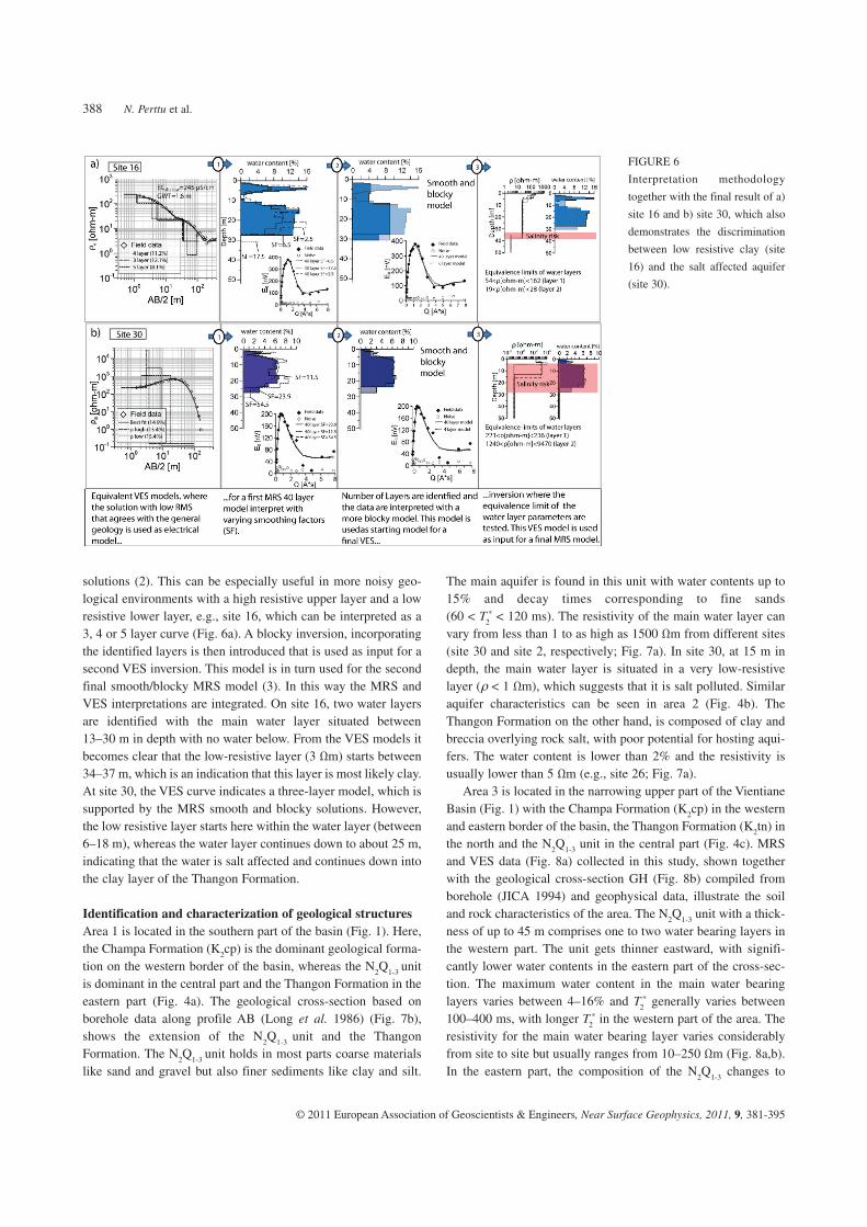
N. Perttu et al.388
© 2011 European Association of Geoscientists & Engineers, Near Surface Geophysics, 2011, 9, 381-395
The main aquifer is found in this unit with water contents up to
15% and decay times corresponding to fine sands
(60 < T2* < 120 ms). The resistivity of the main water layer can
vary from less than 1 to as high as 1500 Ωm from different sites
(site 30 and site 2, respectively; Fig. 7a). In site 30, at 15 m in
depth, the main water layer is situated in a very low-resistive
layer ( < 1 Ωm), which suggests that it is salt polluted. Similar
aquifer characteristics can be seen in area 2 (Fig. 4b). The
Thangon Formation on the other hand, is composed of clay and
breccia overlying rock salt, with poor potential for hosting aqui-
fers. The water content is lower than 2% and the resistivity is
usually lower than 5 Ωm (e.g., site 26; Fig. 7a).
Area 3 is located in the narrowing upper part of the Vientiane
Basin (Fig. 1) with the Champa Formation (K2cp) in the western
and eastern border of the basin, the Thangon Formation (K2tn) in
the north and the N2Q
1-3 unit in the central part (Fig. 4c). MRS
and VES data (Fig. 8a) collected in this study, shown together
with the geological cross-section GH (Fig. 8b) compiled from
borehole (JICA 1994) and geophysical data, illustrate the soil
and rock characteristics of the area. The N2Q
1-3 unit with a thick-
ness of up to 45 m comprises one to two water bearing layers in
the western part. The unit gets thinner eastward, with signifi-
cantly lower water contents in the eastern part of the cross-sec-
tion. The maximum water content in the main water bearing
layers varies between 4–16% and T2* generally varies between
100–400 ms, with longer T2* in the western part of the area. The
resistivity for the main water bearing layer varies considerably
from site to site but usually ranges from 10–250 Ωm (Fig. 8a,b).
In the eastern part, the composition of the N2Q
1-3 changes to
solutions (2). This can be especially useful in more noisy geo-
logical environments with a high resistive upper layer and a low
resistive lower layer, e.g., site 16, which can be interpreted as a
3, 4 or 5 layer curve (Fig. 6a). A blocky inversion, incorporating
the identified layers is then introduced that is used as input for a
second VES inversion. This model is in turn used for the second
final smooth/blocky MRS model (3). In this way the MRS and
VES interpretations are integrated. On site 16, two water layers
are identified with the main water layer situated between
13–30 m in depth with no water below. From the VES models it
becomes clear that the low-resistive layer (3 Ωm) starts between
34–37 m, which is an indication that this layer is most likely clay.
At site 30, the VES curve indicates a three-layer model, which is
supported by the MRS smooth and blocky solutions. However,
the low resistive layer starts here within the water layer (between
6–18 m), whereas the water layer continues down to about 25 m,
indicating that the water is salt affected and continues down into
the clay layer of the Thangon Formation.
Identification and characterization of geological structuresArea 1 is located in the southern part of the basin (Fig. 1). Here,
the Champa Formation (K2cp) is the dominant geological forma-
tion on the western border of the basin, whereas the N2Q
1-3 unit
is dominant in the central part and the Thangon Formation in the
eastern part (Fig. 4a). The geological cross-section based on
borehole data along profile AB (Long et al. 1986) (Fig. 7b),
shows the extension of the N2Q
1-3 unit and the Thangon
Formation. The N2Q
1-3 unit holds in most parts coarse materials
like sand and gravel but also finer sediments like clay and silt.
FIGURE 6
Interpretation methodology
together with the final result of a)
site 16 and b) site 30, which also
demonstrates the discrimination
between low resistive clay (site
16) and the salt affected aquifer
(site 30).
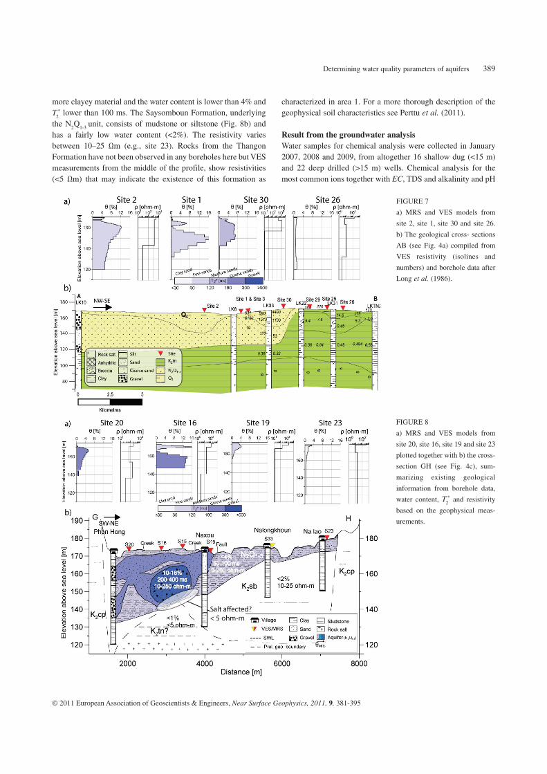
Determining water quality parameters of aquifers 389
© 2011 European Association of Geoscientists & Engineers, Near Surface Geophysics, 2011, 9, 381-395
characterized in area 1. For a more thorough description of the
geophysical soil characteristics see Perttu et al. (2011).
Result from the groundwater analysisWater samples for chemical analysis were collected in January
2007, 2008 and 2009, from altogether 16 shallow dug (<15 m)
and 22 deep drilled (>15 m) wells. Chemical analysis for the
most common ions together with EC, TDS and alkalinity and pH
more clayey material and the water content is lower than 4% and
T2* lower than 100 ms. The Saysomboun Formation, underlying
the N2Q
1-3 unit, consists of mudstone or siltstone (Fig. 8b) and
has a fairly low water content (<2%). The resistivity varies
between 10–25 Ωm (e.g., site 23). Rocks from the Thangon
Formation have not been observed in any boreholes here but VES
measurements from the middle of the profile, show resistivities
(<5 Ωm) that may indicate the existence of this formation as
FIGURE 8
a) MRS and VES models from
site 20, site 16, site 19 and site 23
plotted together with b) the cross-
section GH (see Fig. 4c), sum-
marizing existing geological
information from borehole data,
water content, T2* and resistivity
based on the geophysical meas-
urements.
FIGURE 7
a) MRS and VES models from
site 2, site 1, site 30 and site 26.
b) The geological cross- sections
AB (see Fig. 4a) compiled from
VES resistivity (isolines and
numbers) and borehole data after
Long et al. (1986).
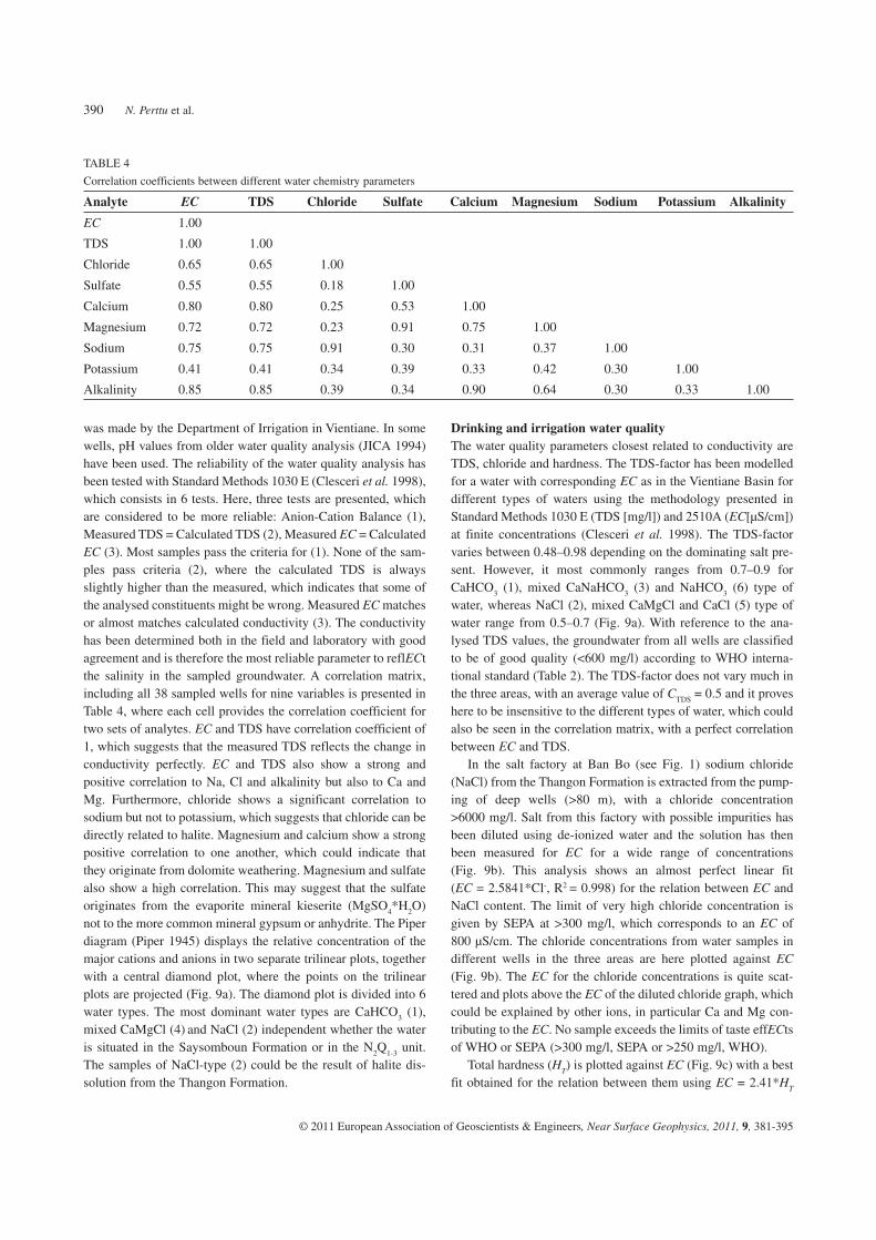
N. Perttu et al.390
© 2011 European Association of Geoscientists & Engineers, Near Surface Geophysics, 2011, 9, 381-395
Drinking and irrigation water qualityThe water quality parameters closest related to conductivity are
TDS, chloride and hardness. The TDS-factor has been modelled
for a water with corresponding EC as in the Vientiane Basin for
different types of waters using the methodology presented in
Standard Methods 1030 E (TDS [mg/l]) and 2510A (EC[μS/cm])
at finite concentrations (Clesceri et al. 1998). The TDS-factor
varies between 0.48–0.98 depending on the dominating salt pre-
sent. However, it most commonly ranges from 0.7–0.9 for
CaHCO3 (1), mixed CaNaHCO
3 (3) and NaHCO
3 (6) type of
water, whereas NaCl (2), mixed CaMgCl and CaCl (5) type of
water range from 0.5–0.7 (Fig. 9a). With reference to the ana-
lysed TDS values, the groundwater from all wells are classified
to be of good quality (<600 mg/l) according to WHO interna-
tional standard (Table 2). The TDS-factor does not vary much in
the three areas, with an average value of CTDS
= 0.5 and it proves
here to be insensitive to the different types of water, which could
also be seen in the correlation matrix, with a perfect correlation
between EC and TDS.
In the salt factory at Ban Bo (see Fig. 1) sodium chloride
(NaCl) from the Thangon Formation is extracted from the pump-
ing of deep wells (>80 m), with a chloride concentration
>6000 mg/l. Salt from this factory with possible impurities has
been diluted using de-ionized water and the solution has then
been measured for EC for a wide range of concentrations
(Fig. 9b). This analysis shows an almost perfect linear fit
(EC = 2.5841*Cl-, R2 = 0.998) for the relation between EC and
NaCl content. The limit of very high chloride concentration is
given by SEPA at >300 mg/l, which corresponds to an EC of
800 μS/cm. The chloride concentrations from water samples in
different wells in the three areas are here plotted against EC
(Fig. 9b). The EC for the chloride concentrations is quite scat-
tered and plots above the EC of the diluted chloride graph, which
could be explained by other ions, in particular Ca and Mg con-
tributing to the EC. No sample exceeds the limits of taste effECts
of WHO or SEPA (>300 mg/l, SEPA or >250 mg/l, WHO).
Total hardness (HT) is plotted against EC (Fig. 9c) with a best
fit obtained for the relation between them using EC = 2.41*HT
was made by the Department of Irrigation in Vientiane. In some
wells, pH values from older water quality analysis (JICA 1994)
have been used. The reliability of the water quality analysis has
been tested with Standard Methods 1030 E (Clesceri et al. 1998),
which consists in 6 tests. Here, three tests are presented, which
are considered to be more reliable: Anion-Cation Balance (1),
Measured TDS = Calculated TDS (2), Measured EC = Calculated
EC (3). Most samples pass the criteria for (1). None of the sam-
ples pass criteria (2), where the calculated TDS is always
slightly higher than the measured, which indicates that some of
the analysed constituents might be wrong. Measured EC matches
or almost matches calculated conductivity (3). The conductivity
has been determined both in the field and laboratory with good
agreement and is therefore the most reliable parameter to reflECt
the salinity in the sampled groundwater. A correlation matrix,
including all 38 sampled wells for nine variables is presented in
Table 4, where each cell provides the correlation coefficient for
two sets of analytes. EC and TDS have correlation coefficient of
1, which suggests that the measured TDS reflects the change in
conductivity perfectly. EC and TDS also show a strong and
positive correlation to Na, Cl and alkalinity but also to Ca and
Mg. Furthermore, chloride shows a significant correlation to
sodium but not to potassium, which suggests that chloride can be
directly related to halite. Magnesium and calcium show a strong
positive correlation to one another, which could indicate that
they originate from dolomite weathering. Magnesium and sulfate
also show a high correlation. This may suggest that the sulfate
originates from the evaporite mineral kieserite (MgSO4*H
2O)
not to the more common mineral gypsum or anhydrite. The Piper
diagram (Piper 1945) displays the relative concentration of the
major cations and anions in two separate trilinear plots, together
with a central diamond plot, where the points on the trilinear
plots are projected (Fig. 9a). The diamond plot is divided into 6
water types. The most dominant water types are CaHCO3 (1),
mixed CaMgCl (4) and NaCl (2) independent whether the water
is situated in the Saysomboun Formation or in the N2Q
1-3 unit.
The samples of NaCl-type (2) could be the result of halite dis-
solution from the Thangon Formation.
TABLE 4
Correlation coefficients between different water chemistry parameters
Analyte EC TDS Chloride Sulfate Calcium Magnesium Sodium Potassium Alkalinity
EC 1.00
TDS 1.00 1.00
Chloride 0.65 0.65 1.00
Sulfate 0.55 0.55 0.18 1.00
Calcium 0.80 0.80 0.25 0.53 1.00
Magnesium 0.72 0.72 0.23 0.91 0.75 1.00
Sodium 0.75 0.75 0.91 0.30 0.31 0.37 1.00
Potassium 0.41 0.41 0.34 0.39 0.33 0.42 0.30 1.00
Alkalinity 0.85 0.85 0.39 0.34 0.90 0.64 0.30 0.33 1.00
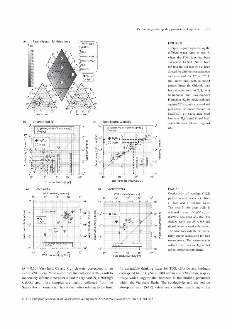
Determining water quality parameters of aquifers 391
© 2011 European Association of Geoscientists & Engineers, Near Surface Geophysics, 2011, 9, 381-395
for acceptable drinking water for TDS, chloride and hardness
correspond to 1200 μS/cm, 800 μS/cm and 720 μS/cm, respec-
tively, which suggest that hardness is the limiting parameter
within the Vientiane Basin. The conductivity and the sodium
absorption ratio (SAR) values are classified according to the
(R2 = 0.70). Very hard, Ca and Mg rich water correspond to an
EC of 720 μS/cm. Most water from the collected wells is soft to
moderately soft but some water is hard to very hard (HT > 300 mg/l
CaCO3) and those samples are mainly collected from the
Saysomboun Formation. The conductivities relating to the limit
FIGURE 9
a) Piper diagram representing the
different water types in area 3,
where the TDS-factor has been
calculated. b) Salt (NaCl) from
the Ban Bo salt factory has been
diluted for different concentration
and measured for EC at 25° C
(full drawn line), with an almost
perfect linear fit. Chloride data
from sampled wells in N2Q
1-3 unit
(diamonds) and Saysomboun
Formation (K2sb) (circles) plotted
against EC are quite scattered and
plot above the linear relation for
NaCl/EC. c) Calculated total
hardness (HT) from Ca2+ and Mg2+
concentrations plotted against
EC.
FIGURE 10
Conductivity of aquifers (VES)
plotted against water EC from
a) deep and b) shallow wells.
The best fit for deep wells is
obtained using EC[μS/cm] =
0.4694VES[μS/cm], R2 = 0.69. For
shallow wells the R2 < 0.3 and
should hence be used with caution.
The error bars indicate the uncer-
tainty due to equivalence for each
measurement. The measurements
without error bars are layers that
are not subject to equivalence.
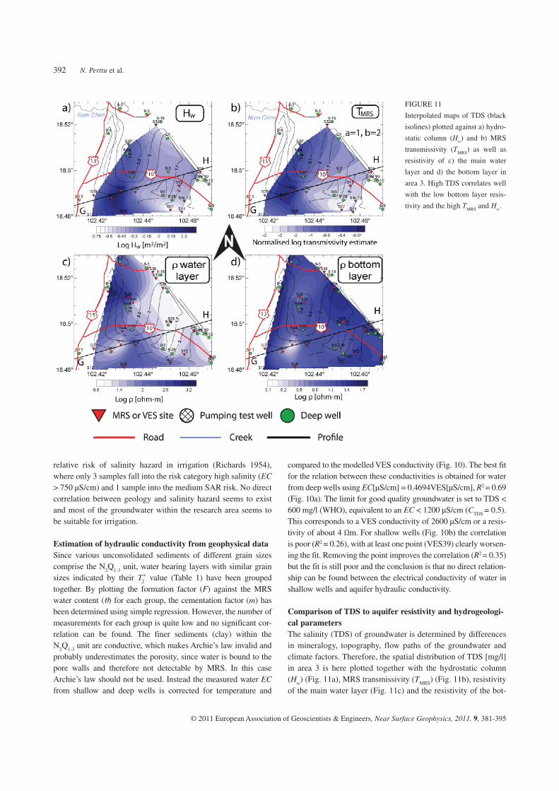
N. Perttu et al.392
© 2011 European Association of Geoscientists & Engineers, Near Surface Geophysics, 2011, 9, 381-395
compared to the modelled VES conductivity (Fig. 10). The best fit
for the relation between these conductivities is obtained for water
from deep wells using EC[μS/cm] = 0.4694VES[μS/cm], R2 = 0.69
(Fig. 10a). The limit for good quality groundwater is set to TDS <
600 mg/l (WHO), equivalent to an EC < 1200 μS/cm (CTDS
= 0.5).
This corresponds to a VES conductivity of 2600 μS/cm or a resis-
tivity of about 4 Ωm. For shallow wells (Fig. 10b) the correlation
is poor (R2 = 0.26), with at least one point (VES39) clearly worsen-
ing the fit. Removing the point improves the correlation (R2 = 0.35)
but the fit is still poor and the conclusion is that no direct relation-
ship can be found between the electrical conductivity of water in
shallow wells and aquifer hydraulic conductivity.
Comparison of TDS to aquifer resistivity and hydrogeologi-cal parametersThe salinity (TDS) of groundwater is determined by differences
in mineralogy, topography, flow paths of the groundwater and
climate factors. Therefore, the spatial distribution of TDS [mg/l]
in area 3 is here plotted together with the hydrostatic column
(Hw) (Fig. 11a), MRS transmissivity (T
MRS) (Fig. 11b), resistivity
of the main water layer (Fig. 11c) and the resistivity of the bot-
relative risk of salinity hazard in irrigation (Richards 1954),
where only 3 samples fall into the risk category high salinity (EC
> 750 μS/cm) and 1 sample into the medium SAR risk. No direct
correlation between geology and salinity hazard seems to exist
and most of the groundwater within the research area seems to
be suitable for irrigation.
Estimation of hydraulic conductivity from geophysical dataSince various unconsolidated sediments of different grain sizes
comprise the N2Q
1-3 unit, water bearing layers with similar grain
sizes indicated by their T2* value (Table 1) have been grouped
together. By plotting the formation factor (F) against the MRS
water content ( ) for each group, the cementation factor (m) has
been determined using simple regression. However, the number of
measurements for each group is quite low and no significant cor-
relation can be found. The finer sediments (clay) within the
N2Q
1-3 unit are conductive, which makes Archie’s law invalid and
probably underestimates the porosity, since water is bound to the
pore walls and therefore not detectable by MRS. In this case
Archie’s law should not be used. Instead the measured water EC
from shallow and deep wells is corrected for temperature and
FIGURE 11
Interpolated maps of TDS (black
isolines) plotted against a) hydro-
static column (Hw) and b) MRS
transmissivity (TMRS
) as well as
resistivity of c) the main water
layer and d) the bottom layer in
area 3. High TDS correlates well
with the low bottom layer resis-
tivity and the high TMRS
and Hw.
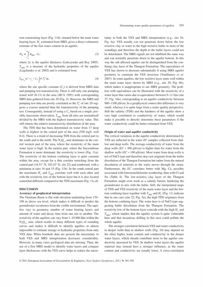
Determining water quality parameters of aquifers 393
© 2011 European Association of Geoscientists & Engineers, Near Surface Geophysics, 2011, 9, 381-395
tainty in both the VES and MRS interpretation (e.g., site 16;
Fig. 6a). VES usually can not penetrate down below the low
resistive clay or water to the high resistive halite in most of the
soundings and therefore the depth to the halite layers could not
be determined. The MRS signals are not inhibited the same way
and can normally penetrate down to the aquifer bottom. In this
way the salt affected aquifer can be distinguished from the con-
fining clay layer of the Thangon Formation. The equivalence of
VES has shown to decrease substantially if using MRS aquifer
geometry to constrain the VES inversion (Vouillamoz et al. 2007). In some aquifers, the low resistive layer starts well within
the main water layer shown by MRS (e.g., site 30; Fig. 6b),
which makes it inappropriate to use MRS geometry. The prob-
lem with equivalence can be illustrated with the resistivity of a
water layer that varies due to equivalence between 9–11 Ωm (site
27; Fig. 10a), corresponding to an aquifer conductivity between
900–1100 μS/cm. In a geophysical context this difference is very
small, whereas it is quite large from a water quality perspective.
Still the salinity (TDS) and the hardness of the aquifer show a
very high correlation to conductivity of water, which would
make it possible to directly determine these parameters if the
water conductivity could be better estimated from VES.
Origin of water and aquifer conductivityThe vertical variations in the aquifer conductivity determined by
VES are reflected in the water EC samples collected from shal-
low and deep wells. The average conductivity of water from the
deep wells (EC ≈ 300 μS/cm) is higher than for water from the
shallow wells (EC ≈ 100 μS/cm). Most water from deep wells is
not of NaCl-type and therefore does not originate from the halite
dissolution of the Thangon Formation but rather from the natural
dissolution of minerals as the water moves through the strata.
Furthermore, the EC correlates better with Mg, Ca, possibly
associated with limestone/dolomite weathering, than with Cl and
Na (Table 4). The low-resistive clay layer of the Thangon
Formation might even work as a salinity barrier, hindering the
groundwater to mix with the halite. Still, the interpolated maps
of TDS and VES resistivity of the main water layer and the bot-
tom confining layer together with TMRS
and Hw (Fig. 11) indicate
that in one case (site 22; Fig. 5a), the high TDS originates from
the bottom confining layer. The water here is of NaCl-type sug-
gesting halite dissolution from the Thangon Formation. The
resistivity low of the bottom layer coincide with the high Hw and
TMRS
, which implies that the aquifer system is quite vulnerable
here and that incautious drilling in this area could pollute the
whole aquifer.
The stronger correlation between VES and water conductivity
in deeper wells than in shallow wells (Fig. 10) may depend on
the often higher water content and conductivity in the deeper
water layers, which should contribute more to the aquifer con-
ductivity measured by VES. In shallow water layers the aquifer
material may instead have a stronger influence, as the water
content and conductivity are usually lower. A cross-correlation
tom constraining layer (Fig. 11d), situated below the main water
bearing layer. Hw estimated from MRS, gives a direct volumetric
estimate of the free water content in an aquifer:
(3)
where Δz is the aquifer thickness (Lubczynski and Roy 2005).
TMRS
is a measure of the hydraulic properties of the aquifer
(Legchenko et al. 2002) and is estimated from
(4)
where the site specific constant (CT) is derived from MRS data
and pumping test transmissivity. There is still only one pumping
tested well (8-13) in the area (JICA 1993) with corresponding
MRS data gathered from site 20 (Fig. 4). However, the MRS and
pumping test data are poorly correlated as the T2* of site 20 sug-
gests a coarser material than the transmissivity of the pumping
test. Consequently, instead of using a CT based on a single, pos-
sibly inaccurate observation, TMRS
from all sites are normalized/
divided by the MRS with the highest transmissivity value. This
still returns the relative transmissivity distribution of the area.
The TDS that has been determined on water from 17 deep
wells is highest in the central part of the area (558 mg/l; well
8-4). There is a trend of decreasing TDS from the central part to
the south and to the north. The N2Q
1-3 unit dominates in the cen-
tral western part of the area, where the resistivity of the main
water layer is high. In the eastern part, where the Saysomboun
Formation is more dominant, the resistivity is lower (Fig. 11a).
The resistivity of the bottom confining layer is quite constant
within the area, except for a thin corridor stretching from the
central part (18.51° N, 102.43° E; site 22) and southward, with a
minimum at sites 16 and 15 (Fig. 11b). In the south central part
the maximum Hw and T
MRS correlate well with each other and
with the resistivity low of the bottom layer but it is also located
somewhat different compared to the TDS maximum (Fig. 11c,d).
DISCUSSIONAccuracy of geophysical interpretationThe Vientiane Basin is flat with elevation undulating from 170–
190 m above sea level, which makes it difficult to predict the
groundwater occurrence from the visible environment. The aqui-
fers vary in geometry, number of water bearing layers and
amount of water and decay time from one site to another. The
resistivity of the aquifers can vary from 1–10 000 m within the
N2Q
1-3 unit, which results in many different types of sounding
curves and makes it difficult to identify aquifers or almost
impossible to estimate storage or hydraulic properties from only
VES data. When borehole data are present the uncertainty in
both VES and MRS interpretation decreases considerably.
However, in many cases geological data are missing. Then, the
use of a first MRS model to identify water layers and compare
layer thicknesses with the VES curve helps to reduce the uncer-
N. Perttu et al.394
© 2011 European Association of Geoscientists & Engineers, Near Surface Geophysics, 2011, 9, 381-395
There is a fairly strong relationship between the conductivity
of water from deep wells and the conductivity of the main water
bearing layer determined by VES, where the best fit is obtained
using: EC[μS/cm] = 0.4694VES[μS/cm], R2 = 0.69. However,
due to equivalence in the VES interpretation and the difficulty to
estimate the resistivity contribution from finer sediments, the
equation may be seen and used as guidance to good water qual-
ity only within the Vientiane Basin or in other areas with similar
geology.
The combination of MRS and VES techniques has been suc-
cessful in distinguishing high conductive clay and mudstone
from water bearing layers and moreover freshwater aquifers
from salt affected water. Furthermore, the combination of MRS
and VES allows also identifying water layers in the VES curve
and constraining the number of possible MRS and VES solutions
and hence decreasing the uncertainty in the interpretation.
Altogether, this makes MRS and VES very promising tools for
guidance of future drillings and water quality estimation.
ACKNOWLEDGEMENTSThis study was funded by the Swedish International Development
Cooperation Agency (SIDA-SAREC). The authors acknowledge
the National University of Laos (NUoL) for invaluable help and
support before and during field work, making this project a real-
ity. A special thanks to the Department of Geology and Mining
and JICA, who provided invaluable data and the Department of
Irrigation for analysing our water samples. Our deepest apprecia-
tion goes to Sounthone Singsoupho, Viengthong Xayavong,
Titusadewale Olowokudejo and Sengthong Bounyavongand for
field assistance and Fredrik Nordblad for lending out and prepar-
ing the Hanna Instrument for us. We would also like to thank the
anonymous reviewers for their comments and suggestions that
really helped to improve the paper.
REFERENCESAllen D., Andreani M., Badry R., Flaum C., Gossenberg P., Horkowitz J.,
Singer J. and White J. 1997. How to use borehole NMR. Oil Review
(Summer), 34–57.
Archie G.E. 1942. The electrical resistivity log as an aid in determining
some reservoir characteristics. Metallurgical and Petroleum Engineers
146, 54–62.
Back W. and Hanshaw B.B. 1965. Chemical geohydrology. Advances in Hydroscience 2, 49–109.
Clesceri L.S.E., Greenberg A.E.E. and Eaton A.D.E. 1998. Standard Methods for the Examination of Water and Wastewater. American
Public Health Association (Washington), American Water Works
Association (Denver) and Water Environment Federation (Alexandria,
VA).
El Tabakh M., Utha-Aroon C. and Schreiber B.C. 1999. Sedimentology
of the Cretaceous Maha Sarakham evaporites in the Khorat Plateau of
northeastern Thailand. Sedimentary Geology 123, 31–62.
Gibbs R. 1970. Mechanisms controlling world water chemistry. Science
170, 1088–1090.
Hertrich M. 2008. Imaging of groundwater with nuclear magnetic reso-
nance. Progress in Nuclear Magnetic Resonance Spectroscopy 53,
227–248.
between water and aquifer conductivity (Fig. 10) does not
express a possible influence from the aquifer material. Waxman
and Smits (1968) provided a model for current flow in porous,
clayey media, where one part of the aquifer conductivity is
related to the pore water and the other part is associated with the
cation exchange capacity (i.e., clay). The aquifer conductivity is
then the sum of the two. Analogous to their model, it might be
possible to roughly estimate the contribution from the finer sedi-
ments/clay using the relaxation time retrieved from MRS. Here,
the T2* from the VES constrained MRS models have been used.
However, no such indication of serial autocorrelation exists in
the data from the Vientiane area. This could be explained from
the fact that T2* has proven to be difficult to evaluate correctly for
low water contents and especially clayey material. A combina-
tion of VES and induced polarization (IP) could also be used to
better evaluate the relationship between aquifer and water resis-
tivity. However, the relationship between chargeability and clay
content is quite complex (Worthington and Collar 1982) and the
IP data collected in this study were of too poor quality to be used.
Back and Hanshaw (1965) stated that an aquifer with fine
grained material has higher content of dissolved solids than an
aquifer with coarser material. Therefore, finer sediments play an
important role not just in estimation of the aquifer resistivity but
probably also in the composition of the groundwater. Future
research on decay time could help in better estimating the contri-
bution from aquifer material but also in understanding the inter-
action between finer sediments and groundwater quality.
CONCLUSIONSThe main water bearing unit in the Vientiane Basin (N
2Q
1-3) is
characterized by relatively high water contents with decay times
suggesting a mean pore size equivalent to fine sand and gravel
The resistivity of the aquifers is highly variable but is most often
above 4 m, suggesting predominantly fresh water. The salt car-
rying Thangon Formation is usually found beneath N2Q
1-3 and is
characterized by a low resistive clay layer with no free water. The
main water quality parameters affecting the water conductivity
are TDS and hardness and to a minor extent chloride, which all
have shown to have fairly high correlation to the EC of ground-
water. The correlation factors controlling these relationships are
dependent on the type of water present and should therefore be
accounted for if the water quality parameters of the aquifer are to
be determined correctly. None of the wells in the investigated
areas have water quality parameters exceeding the limit for unac-
ceptable drinking or irrigation water, although the hardness and
chloride content in some wells exceed the esthetical and techni-
cal limit. Still, the TDS contour maps plotted over the resistivity
of the main aquifer in area 3 and the layer beneath confining the
aquifer together with MRS parameters like hydrostatic column
and transmissivity show the vulnerability of the aquifer. Here,
the aquifer containing most water with highest transmissivity is
found over a very low restive layer, probably associated with salt
polluted clay of the Thangon Formation.
Determining water quality parameters of aquifers 395
© 2011 European Association of Geoscientists & Engineers, Near Surface Geophysics, 2011, 9, 381-395
Perttu N., Wattanasen K., Phommasone K. and Elming S-Å. 2011.
Characterization of aquifers in the Vientiane Basin, Laos, using mag-
netic resonance sounding and vertical electrical sounding. Journal of Applied Geophysics 73, 207–220. doi:10.1016/j.jappgeo.2011.01.003
Piper A. 1945. A graphic procedure in the geochemical interpretation of
water-analyses. American Geophysical Union Transactions 25, 914–
923.
Reynolds T. and Richards P. 1996. Unit Operations and Processes in Environmental Engineering. PWS Publishing Company.
Richards L.A. 1954. Diagnosis and Improvement of Saline and Alkali Soils. US Salinity Laboratory Staff, Washington.
SEPA 2000. Environmental Quality Criteria – Groundwater. Report
5051, Swedish Environmental Protection Agency (SEPA), Kalmar.
Shirov, M., Legchenko A. and Creer G. 1991. A new direct non-invasive
groundwater detection technology for Australia. Exploration Geophysics 22, 333–338.
Shoeller H. 1959. Arid Zone Hydrology: Recent Developments.
UNESCO.
Srisuk K., Sriboonlue V. and Buaphan C. 1999. Groundwater flow, saline
water and saline soils in the Central Khorat Basin, northeast Thailand.
Symposium on Mineral, Energy and Water Resources of Thailand: Towards the year 2000, Chulalongkorn University, Bangkok, Thailand,
28–29 October 1999, 238–251.
STEA 2001. State of the Environment Report. 2001: Lao People’s Democratic Republic. UNEP, RRC.AP.
Sundberg K. 1932. Effect of impregnating waters on conductivity of soils
and rocks. AIME 97, 367–391.
US Salinity Laboratory Staff 1954. Diagnosis and Improvement of Saline and Alkali Soils. USDA, Washington, DC.
Vouillamoz J.M., Chatenoux B., Mathieu F., Baltassat J.M. and
Legchenko A. 2007. Efficiency of joint use of MRS and VES to char-
acterize a coastal aquifer in Myanmar. Journal of Applied Geophysics
61, 142–154.
Vouillamoz J.M., Descloitres M., Bernard J., Fourcassier P. and Romagny
L. 2002. Application of integrated magnetic resonance sounding and
resistivity methods for borehole implementation. A case study in
Cambodia. Journal of Applied Geophysics 50, 67–81.
Wannakomol A. 2005. Soil and groundwater salinization problems in the Khorat Plateau, NE Thailand, integrated study of remote sensing, geophysical and field data. PhD thesis, Free University of Berlin.
Waxman M.H. and Smits L.J.H. 1968. Electrical conductivities in oil-bearing shale sands. SPE Journal 243, 107–122.
WHO 1996. Guidelines for Drinking-water Quality, 3rd edn, incorporat-
ing first and second addenda, Volume 1 Recommendations.
Williamson D.R., Peck A.J., Turner J.V. and Arunin S. 1989. Groundwater
hydrology and salinity in a valley in Northeast Thailand. Groundwater Contamination IAHS-AISH Publication 185, 147–154.
Worthington P. 1993. The uses and abuses of the Archie equations. 1 –
The formation factor-porosity relationship. Journal of Applied Geophysics 30, 215–228.
Worthington P. and Collar F.A. 1982. The relevance of induced polariza-
tion to quantitative formation evaluation. Transactions of the SPWLA
Annual Logging Symposium, 23.
JICA 1993. Design study report on the Project for Groundwater
Development in Vientiane Province in Lao People’s Democratic
Republic. Japan International Cooperation Agency (JICA).
JICA 1994. Drilling logs from the “Groundwater Development in the
Vientiane Province Project”. Japan International Cooperation Agency
(JICA), JICA Local Office in Phon Hong, Vientiane Province, Laos.
JICA 2000. The study on rural water supply and sanitation improvement
in the northwest region in the Lao People´s Democratic Republic.
Progress report 2, Japan International Cooperation Agency (JICA).
Krawczyk W.E. and Ford D.C. 2006. Correlating specific conductivity
with total hardness in limestone and dolomite karst waters. Earth Surface Processes and Landforms 31, 221–234.
Krawczyk W.E. and Ford D.C. 2007. Correlating specific conductivity
with total hardness in gypsum karst waters. Earth Surface Processes and Landforms 32, 612–620.
Legchenko A. 2005. Improved modelling of the magnetic resonance
signal in the presence of shallow aquifers. Near Surface Geophysics 3,
121–130.
Legchenko A. 2007. MRS measurements and inversion in presence of
EM noise. Boletin Geológico y Minero 118, 489–508.
Legchenko A., Baltassat J.M., Beauce A. and Bernard J. 2002. Nuclear
magnetic resonance as a geophysical tool for hydrogeologists. Journal of Applied Geophysics 50, 21–46.
Legchenko A. and Valla P. 1998. Processing of surface proton magnetic
resonance signals using non-linear fitting. Journal of Applied Geophysics 39, 77–83.
Legchenko A. and Valla P. 2002. A review of the basic principles for
proton magnetic resonance sounding measurements. Journal of Applied Geophysics 50, 3–19.
Legchenko A. and Valla P. 2003. Removal of power-line harmonics from
proton magnetic resonance measurements. Journal of Applied Geophysics 53, 103–120.
Limpinuntana V. and Arunin S. 1986. Salt affected land in Thailand and
its agricultural productivity. Reclamation and Revegation Research 5,
143–149.
Löffler E. and Kubiniok J. 1986. Soil salinization in north-east Thailand.
Erdkunde 42, 89–100.
Long N.X., Lam N.X. and Canh N.D. 1986. Report on geological data
for Potassium and Manganese in Thangon Region, Dong Bang,
Vientiane. Department of Geology and Mining, Vientiane, Laos.
Lovatt Smith P.F., Stokes R.B., Bristow C. and Carter A. 1996. Mid-
Cretaceous inversion in the northern Khorat Plateau of Lao PDR and
Thailand. In: Tectonic Evolution of Southeast Asia (eds R. Hall and D.
Blundell), pp. 233–247. Geological Society of London.
Lubczynski M. and Roy J. 2003. Hydrogeological interpretation and
potential of the new magnetic resonance sounding (MRS) method.
Journal of Hydrology 283, 19–40.
Lubczynski M. and Roy J. 2005. MRS contribution to hydrogeological
system parametrization. Near Surface Geophysics 3, 131–139.
Medlicott K. 2001. Water, sanitation and environmental health in rural
Laos PDR. KAP Study for UNICEF, WES Section.

Paper III
Magnetic Resonance Sounding and Radiomagnetotelluric measurements used to characterize a limestone aquifer in Gotland, Sweden.
Perttu, N., Persson, L., Erlström, M. and Elming, S-Å. (2011) Submitted to Journal of Hydrology

1
Magnetic Resonance Sounding and Radiomagnetotelluric measurements used to characterize a limestone aquifer in Gotland, SwedenNils Perttu1,*, Lena Persson2, Mikael Erlström2, Sten-Åke Elming1
1Division of Ore Geology and Applied Geophysics, Luleå University of Technology, SE-971 87 Luleå, Sweden
2Geological Survey of Sweden, PO Box 670, SE-751 28 Uppsala, Sweden
*Corresponding author: [email protected], Tel: +46-920-491884, Fax: +46-920-491199
AbstractAlmost all drinking water in Gotland is groundwater and is mainly found in karst limestone. However, the unpredictable location and geometry of the karst cracks and caverns makes it very difficult to estimate groundwater storage and movement, as well as contaminant transport. The aim of this study was to test the performance of different geophysical techniques like Magnetic Resonance Sounding (MRS), Radiomagnetotelluric (RMT), Vertical Electrical Sounding (VES), Ground Penetrating Radar (GPR) to characterize aquifers in Gotland, in respect to geometry and storage as well as connectivity over a wider area. The investigated area is located on the south-eastern part of Gotland, about 10 km north-west of the village Ljugarn. The geology here is dominated by 50 to 60 m thick successions of limestone that gradually turn into marlstone. The use of multiple techniques has shown to give a more coherent interpretation. However, the shallow penetration depth of GPR and the lack of soil cover in some places of the investigated area limit the use of geoelectrical methods and GPR. With MRS, the main water layers were identifies at depths between 10 and 60 m and with maximum water content at depths of 20 to 30 m, which coincides with the most resistive sections of the limestone. The water content varies between 0 and 5 %, with a relaxation time (T1MRS) less than 400 ms suggesting that the aquifer is hosted in small fractures, molds and vugs rather than larger karst fractures and caverns. Two potential aquifers were identified with MRS, possibly separated by marlstone. From modelling it can be seen that such boundary separating two aquifer apart can be more easily discriminated in the N/S-, than in the E/W direction. In summary, MRS is therefore the only method in this survey that can detect and determine the vertical and lateral distribution of water within the aquifer together with the total volume of free water. The RMT method has shown effective in characterizing the limestone/marl interface, but also to locate anomalous low resistive zones, possibly associated with salt water. RMT also helps to constrain the final MRS model by choosing a suitable regularization for the MRS 3D inversion. All together, the combination of MRS and RMT seems most efficient and promising for future groundwater explorations on Gotland.
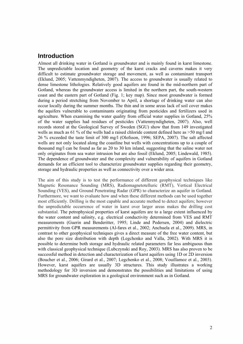
2
IntroductionAlmost all drinking water in Gotland is groundwater and is mainly found in karst limestone. The unpredictable location and geometry of the karst cracks and caverns makes it very difficult to estimate groundwater storage and movement, as well as contaminant transport (Eklund, 2005; Vattenmyndigheten, 2007). The access to groundwater is usually related to dense limestone lithologies. Relatively good aquifers are found in the mid-northern part of Gotland, whereas the groundwater access is limited in the northern part, the south-western coast and the eastern part of Gotland (Fig. 1; key map). Since most groundwater is formed during a period stretching from November to April, a shortage of drinking water can also occur locally during the summer months. The thin and in some areas lack of soil cover makes the aquifers vulnerable to contaminants originating from pesticides and fertilizers used in agriculture. When examining the water quality from official water supplies in Gotland, 25% of the water supplies had residues of pesticides (Vattenmyndigheten, 2007). Also, well records stored at the Geological Survey of Sweden (SGU) show that from 149 investigated wells as much as 61 % of the wells had a raised chloride content defined here as >50 mg/l and 26 % exceeded the taste limit of 300 mg/l (Olofsson, 1996; SEPA, 2007). The salt affected wells are not only located along the coastline but wells with concentrations up to a couple of thousand mg/l can be found as far as 20 to 30 km inland, suggesting that the saline water not only originates from sea water intrusion but are also fossil (Eklund, 2005; Lindewald, 1985). The dependence of groundwater and the complexity and vulnerability of aquifers in Gotland demands for an efficient tool to characterize groundwater supplies regarding their geometry, storage and hydraulic properties as well as connectivity over a wider area.
The aim of this study is to test the performance of different geophysical techniques like Magnetic Resonance Sounding (MRS), Radiomagnetotelluric (RMT), Vertical Electrical Sounding (VES), and Ground Penetrating Radar (GPR) to characterize an aquifer in Gotland. Furthermore, we want to evaluate how and when these different methods can be used together most efficiently. Drilling is the most capable and accurate method to detect aquifers; however the unpredictable occurrence of water in karst over larger areas makes the drilling cost substantial. The petrophysical properties of karst aquifers are to a large extent influenced by the water content and salinity, e.g. electrical conductivity determined from VES and RMT measurements (Guerin and Benderitter, 1995; Linde and Pedersen, 2004) and dielectric permittivity from GPR measurements (Al-fares et al., 2002; Anchuela et al., 2009). MRS, in contrast to other geophysical techniques gives a direct measure of the free water content, but also the pore size distribution with depth (Legchenko and Valla, 2002). With MRS it is possible to determine both storage and hydraulic related parameters far less ambiguous than with classical geophysical technique (Lubczynski and Roy, 2003). MRS has also proven to be successful method in detection and characterization of karst aquifers using 1D or 2D inversion (Boucher et al., 2006; Girard et al., 2007; Legchenko et al., 2008; Vouillamoz et al., 2003). However, karst aquifers are usually 3D structures. This study illustrates a working methodology for 3D inversion and demonstrates the possibilities and limitations of using MRS for groundwater exploration in a geological environment such as in Gotland.
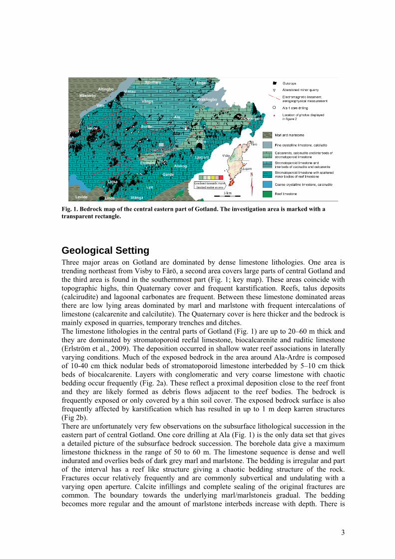
3
Fig. 1. Bedrock map of the central eastern part of Gotland. The investigation area is marked with a transparent rectangle.
Geological Setting Three major areas on Gotland are dominated by dense limestone lithologies. One area is trending northeast from Visby to Fårö, a second area covers large parts of central Gotland and the third area is found in the southernmost part (Fig. 1; key map). These areas coincide with topographic highs, thin Quaternary cover and frequent karstification. Reefs, talus deposits (calcirudite) and lagoonal carbonates are frequent. Between these limestone dominated areas there are low lying areas dominated by marl and marlstone with frequent intercalations of limestone (calcarenite and calcilutite). The Quaternary cover is here thicker and the bedrock is mainly exposed in quarries, temporary trenches and ditches. The limestone lithologies in the central parts of Gotland (Fig. 1) are up to 20–60 m thick and they are dominated by stromatoporoid reefal limestone, biocalcarenite and ruditic limestone (Erlström et al., 2009). The deposition occurred in shallow water reef associations in laterally varying conditions. Much of the exposed bedrock in the area around Ala-Ardre is composed of 10-40 cm thick nodular beds of stromatoporoid limestone interbedded by 5–10 cm thick beds of biocalcarenite. Layers with conglomeratic and very coarse limestone with chaotic bedding occur frequently (Fig. 2a). These reflect a proximal deposition close to the reef front and they are likely formed as debris flows adjacent to the reef bodies. The bedrock is frequently exposed or only covered by a thin soil cover. The exposed bedrock surface is also frequently affected by karstification which has resulted in up to 1 m deep karren structures (Fig 2b). There are unfortunately very few observations on the subsurface lithological succession in the eastern part of central Gotland. One core drilling at Ala (Fig. 1) is the only data set that gives a detailed picture of the subsurface bedrock succession. The borehole data give a maximum limestone thickness in the range of 50 to 60 m. The limestone sequence is dense and well indurated and overlies beds of dark grey marl and marlstone. The bedding is irregular and part of the interval has a reef like structure giving a chaotic bedding structure of the rock. Fractures occur relatively frequently and are commonly subvertical and undulating with a varying open aperture. Calcite infillings and complete sealing of the original fractures are common. The boundary towards the underlying marl/marlstoneis gradual. The bedding becomes more regular and the amount of marlstone interbeds increase with depth. There is
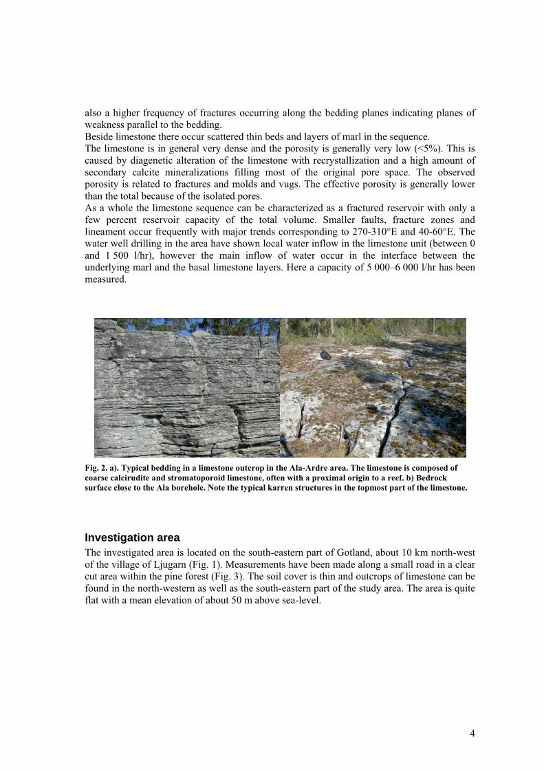
4
also a higher frequency of fractures occurring along the bedding planes indicating planes of weakness parallel to the bedding. Beside limestone there occur scattered thin beds and layers of marl in the sequence. The limestone is in general very dense and the porosity is generally very low (<5%). This is caused by diagenetic alteration of the limestone with recrystallization and a high amount of secondary calcite mineralizations filling most of the original pore space. The observed porosity is related to fractures and molds and vugs. The effective porosity is generally lower than the total because of the isolated pores. As a whole the limestone sequence can be characterized as a fractured reservoir with only a few percent reservoir capacity of the total volume. Smaller faults, fracture zones and lineament occur frequently with major trends corresponding to 270-310°E and 40-60°E. The water well drilling in the area have shown local water inflow in the limestone unit (between 0 and 1 500 l/hr), however the main inflow of water occur in the interface between the underlying marl and the basal limestone layers. Here a capacity of 5 000–6 000 l/hr has been measured.
Fig. 2. a). Typical bedding in a limestone outcrop in the Ala-Ardre area. The limestone is composed of coarse calcirudite and stromatoporoid limestone, often with a proximal origin to a reef. b) Bedrock surface close to the Ala borehole. Note the typical karren structures in the topmost part of the limestone.
Investigation area The investigated area is located on the south-eastern part of Gotland, about 10 km north-west of the village of Ljugarn (Fig. 1). Measurements have been made along a small road in a clear cut area within the pine forest (Fig. 3). The soil cover is thin and outcrops of limestone can be found in the north-western as well as the south-eastern part of the study area. The area is quite flat with a mean elevation of about 50 m above sea-level.
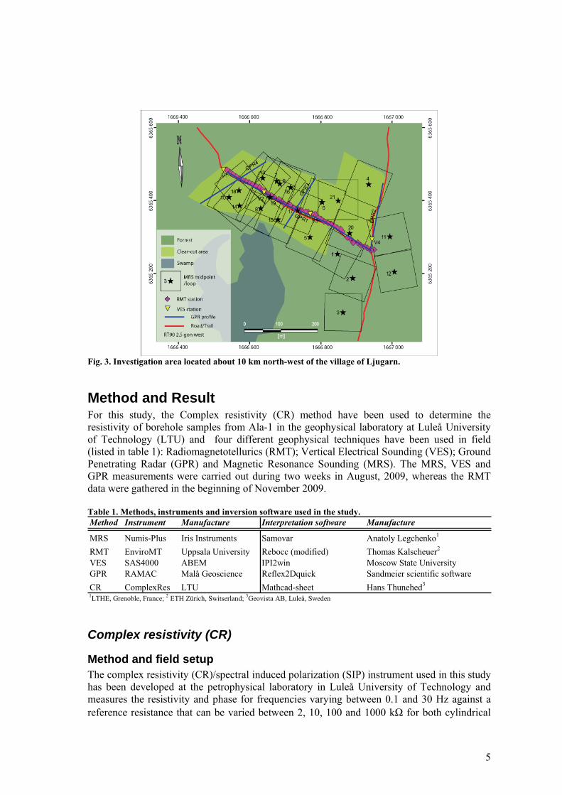
5
Fig. 3. Investigation area located about 10 km north-west of the village of Ljugarn.
Method and Result For this study, the Complex resistivity (CR) method have been used to determine the resistivity of borehole samples from Ala-1 in the geophysical laboratory at Luleå University of Technology (LTU) and four different geophysical techniques have been used in field (listed in table 1): Radiomagnetotellurics (RMT); Vertical Electrical Sounding (VES); Ground Penetrating Radar (GPR) and Magnetic Resonance Sounding (MRS). The MRS, VES and GPR measurements were carried out during two weeks in August, 2009, whereas the RMT data were gathered in the beginning of November 2009.
Table 1. Methods, instruments and inversion software used in the study. Method Instrument Manufacture Interpretation software Manufacture
MRS Numis-Plus Iris Instruments Samovar Anatoly Legchenko1
RMT EnviroMT Uppsala University Rebocc (modified) Thomas Kalscheuer2
VES SAS4000 ABEM IPI2win Moscow State University GPR RAMAC Malå Geoscience Reflex2Dquick Sandmeier scientific software CR ComplexRes LTU Mathcad-sheet Hans Thunehed3
1LTHE, Grenoble, France; 2 ETH Zürich, Switserland; 3Geovista AB, Luleå, Sweden
Complex resistivity (CR)
Method and field setup The complex resistivity (CR)/spectral induced polarization (SIP) instrument used in this study has been developed at the petrophysical laboratory in Luleå University of Technology and measures the resistivity and phase for frequencies varying between 0.1 and 30 Hz against a reference resistance that can be varied between 2, 10, 100 and 1000 k for both cylindrical
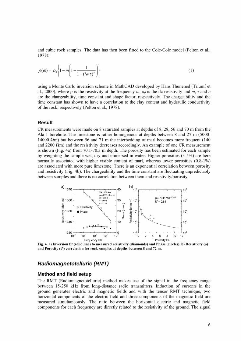
6
and cubic rock samples. The data has then been fitted to the Cole-Cole model (Pelton et al., 1978):
cim
)(1111)( 0 (1)
using a Monte Carlo inversion scheme in MathCAD developed by Hans Thunehed (Triumf et al., 2000), where is the resistivity at the frequency , 0 is the dc resistivity and m, and care the chargeability, time constant and shape factor, respectively. The chargeability and the time constant has shown to have a correlation to the clay content and hydraulic conductivity of the rock, respectively (Pelton et al., 1978).
ResultCR measurements were made on 8 saturated samples at depths of 8, 28, 56 and 70 m from the Ala-1 borehole. The limestone is rather homogenous at depths between 8 and 27 m (5000- 14000 m) but between 56 and 71 m the interbedding of marl becomes more frequent (140 and 2200 m) and the resistivity decreases accordingly. An example of one CR measurement is shown (Fig. 4a) from 70.1-70.3 m depth. The porosity has been estimated for each sample by weighting the sample wet, dry and immersed in water. Higher porosities (3-5%) are here normally associated with higher visible content of marl, whereas lower porosities (0.8-1%) are associated with more pure limestone. There is an exponential correlation between porosity and resistivity (Fig. 4b). The chargeability and the time constant are fluctuating unpredictably between samples and there is no correlation between them and resistivity/porosity.
Fig. 4. a) Inversion fit (solid line) to measured resistivity (diamonds) and Phase (circles). b) Resistivity ( )and Porosity ( ) correlation for rock samples at depths between 8 and 72 m.
Radiomagnetotelluric (RMT)
Method and field setup The RMT (Radiomagnetotelluric) method makes use of the signal in the frequency range between 15-250 kHz from long-distance radio transmitters. Induction of currents in the ground generates electric and magnetic fields and with the tensor RMT technique, two horizontal components of the electric field and three components of the magnetic field are measured simultaneously. The ratio between the horizontal electric and magnetic field components for each frequency are directly related to the resistivity of the ground. The signal
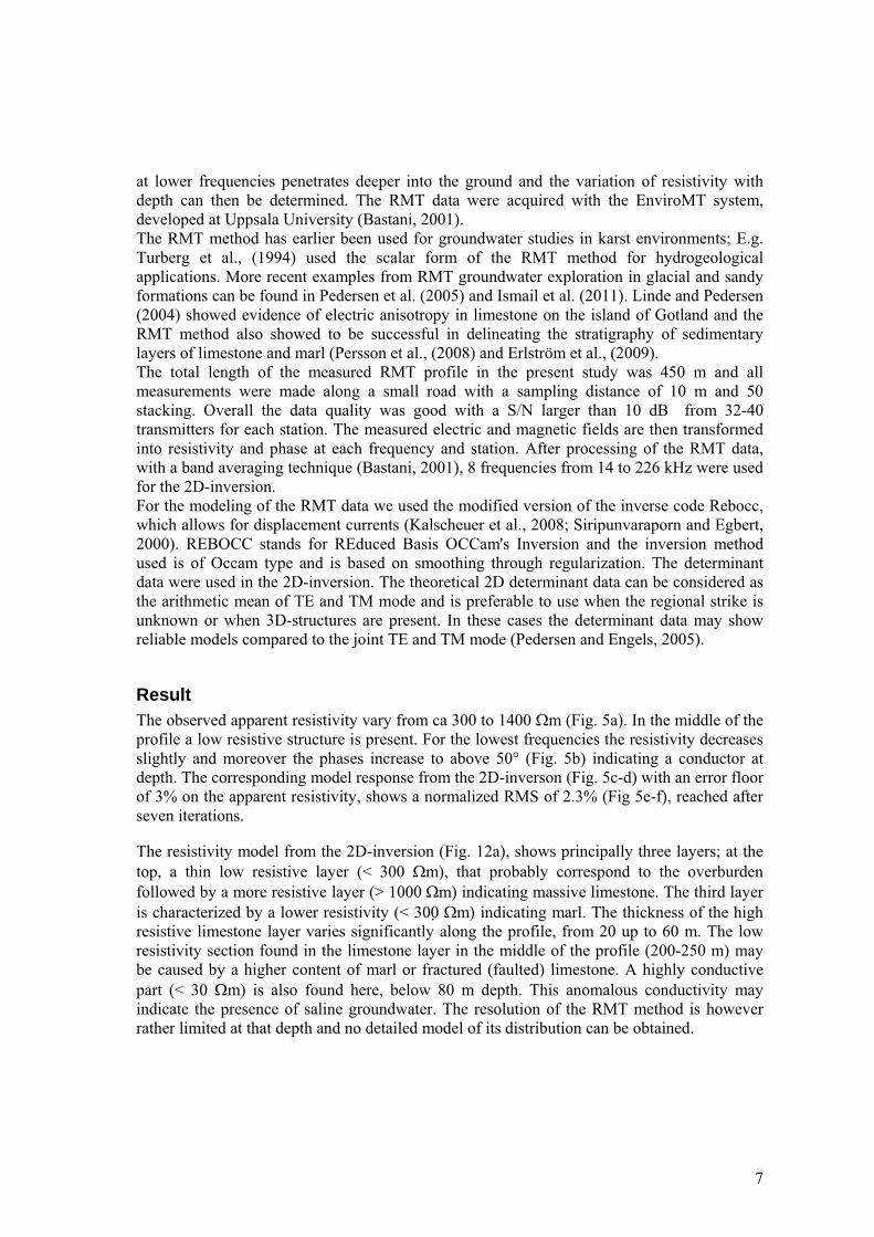
7
at lower frequencies penetrates deeper into the ground and the variation of resistivity with depth can then be determined. The RMT data were acquired with the EnviroMT system, developed at Uppsala University (Bastani, 2001). The RMT method has earlier been used for groundwater studies in karst environments; E.g. Turberg et al., (1994) used the scalar form of the RMT method for hydrogeological applications. More recent examples from RMT groundwater exploration in glacial and sandy formations can be found in Pedersen et al. (2005) and Ismail et al. (2011). Linde and Pedersen (2004) showed evidence of electric anisotropy in limestone on the island of Gotland and the RMT method also showed to be successful in delineating the stratigraphy of sedimentary layers of limestone and marl (Persson et al., (2008) and Erlström et al., (2009). The total length of the measured RMT profile in the present study was 450 m and all measurements were made along a small road with a sampling distance of 10 m and 50 stacking. Overall the data quality was good with a S/N larger than 10 dB from 32-40 transmitters for each station. The measured electric and magnetic fields are then transformed into resistivity and phase at each frequency and station. After processing of the RMT data, with a band averaging technique (Bastani, 2001), 8 frequencies from 14 to 226 kHz were used for the 2D-inversion. For the modeling of the RMT data we used the modified version of the inverse code Rebocc, which allows for displacement currents (Kalscheuer et al., 2008; Siripunvaraporn and Egbert, 2000). REBOCC stands for REduced Basis OCCam's Inversion and the inversion method used is of Occam type and is based on smoothing through regularization. The determinant data were used in the 2D-inversion. The theoretical 2D determinant data can be considered as the arithmetic mean of TE and TM mode and is preferable to use when the regional strike is unknown or when 3D-structures are present. In these cases the determinant data may show reliable models compared to the joint TE and TM mode (Pedersen and Engels, 2005).
ResultThe observed apparent resistivity vary from ca 300 to 1400 m (Fig. 5a). In the middle of the profile a low resistive structure is present. For the lowest frequencies the resistivity decreases slightly and moreover the phases increase to above 50° (Fig. 5b) indicating a conductor at depth. The corresponding model response from the 2D-inverson (Fig. 5c-d) with an error floor of 3% on the apparent resistivity, shows a normalized RMS of 2.3% (Fig 5e-f), reached after seven iterations.
The resistivity model from the 2D-inversion (Fig. 12a), shows principally three layers; at the top, a thin low resistive layer (< 300 m), that probably correspond to the overburden followed by a more resistive layer (> 1000 m) indicating massive limestone. The third layer is characterized by a lower resistivity (< 300 m) indicating marl. The thickness of the high resistive limestone layer varies significantly along the profile, from 20 up to 60 m. The low resistivity section found in the limestone layer in the middle of the profile (200-250 m) may be caused by a higher content of marl or fractured (faulted) limestone. A highly conductive part (< 30 m) is also found here, below 80 m depth. This anomalous conductivity may indicate the presence of saline groundwater. The resolution of the RMT method is however rather limited at that depth and no detailed model of its distribution can be obtained.
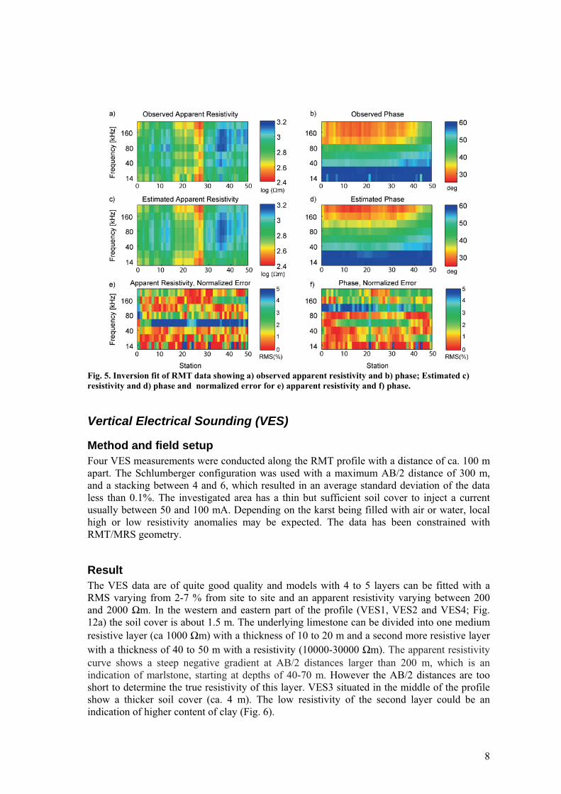
8
Fig. 5. Inversion fit of RMT data showing a) observed apparent resistivity and b) phase; Estimated c) resistivity and d) phase and normalized error for e) apparent resistivity and f) phase.
Vertical Electrical Sounding (VES)
Method and field setup Four VES measurements were conducted along the RMT profile with a distance of ca. 100 m apart. The Schlumberger configuration was used with a maximum AB/2 distance of 300 m, and a stacking between 4 and 6, which resulted in an average standard deviation of the data less than 0.1%. The investigated area has a thin but sufficient soil cover to inject a current usually between 50 and 100 mA. Depending on the karst being filled with air or water, local high or low resistivity anomalies may be expected. The data has been constrained with RMT/MRS geometry.
ResultThe VES data are of quite good quality and models with 4 to 5 layers can be fitted with a RMS varying from 2-7 % from site to site and an apparent resistivity varying between 200 and 2000 m. In the western and eastern part of the profile (VES1, VES2 and VES4; Fig. 12a) the soil cover is about 1.5 m. The underlying limestone can be divided into one medium resistive layer (ca 1000 m) with a thickness of 10 to 20 m and a second more resistive layer with a thickness of 40 to 50 m with a resistivity (10000-30000 m). The apparent resistivity curve shows a steep negative gradient at AB/2 distances larger than 200 m, which is an indication of marlstone, starting at depths of 40-70 m. However the AB/2 distances are too short to determine the true resistivity of this layer. VES3 situated in the middle of the profile show a thicker soil cover (ca. 4 m). The low resistivity of the second layer could be an indication of higher content of clay (Fig. 6).
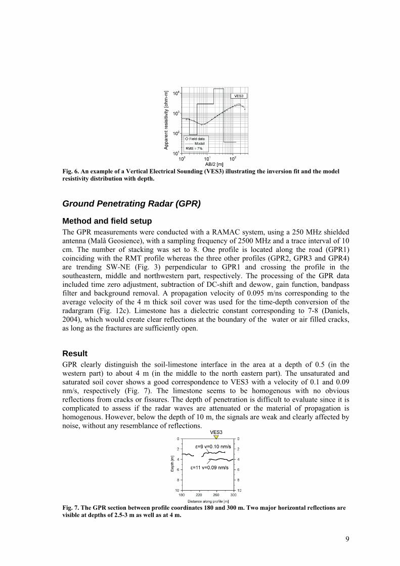
9
Fig. 6. An example of a Vertical Electrical Sounding (VES3) illustrating the inversion fit and the model resistivity distribution with depth.
Ground Penetrating Radar (GPR)
Method and field setup The GPR measurements were conducted with a RAMAC system, using a 250 MHz shielded antenna (Malå Geosience), with a sampling frequency of 2500 MHz and a trace interval of 10 cm. The number of stacking was set to 8. One profile is located along the road (GPR1) coinciding with the RMT profile whereas the three other profiles (GPR2, GPR3 and GPR4) are trending SW-NE (Fig. 3) perpendicular to GPR1 and crossing the profile in the southeastern, middle and northwestern part, respectively. The processing of the GPR data included time zero adjustment, subtraction of DC-shift and dewow, gain function, bandpass filter and background removal. A propagation velocity of 0.095 m/ns corresponding to the average velocity of the 4 m thick soil cover was used for the time-depth conversion of the radargram (Fig. 12c). Limestone has a dielectric constant corresponding to 7-8 (Daniels, 2004), which would create clear reflections at the boundary of the water or air filled cracks, as long as the fractures are sufficiently open.
ResultGPR clearly distinguish the soil-limestone interface in the area at a depth of 0.5 (in the western part) to about 4 m (in the middle to the north eastern part). The unsaturated and saturated soil cover shows a good correspondence to VES3 with a velocity of 0.1 and 0.09 nm/s, respectively (Fig. 7). The limestone seems to be homogenous with no obvious reflections from cracks or fissures. The depth of penetration is difficult to evaluate since it is complicated to assess if the radar waves are attenuated or the material of propagation is homogenous. However, below the depth of 10 m, the signals are weak and clearly affected by noise, without any resemblance of reflections.
Fig. 7. The GPR section between profile coordinates 180 and 300 m. Two major horizontal reflections are visible at depths of 2.5-3 m as well as at 4 m.
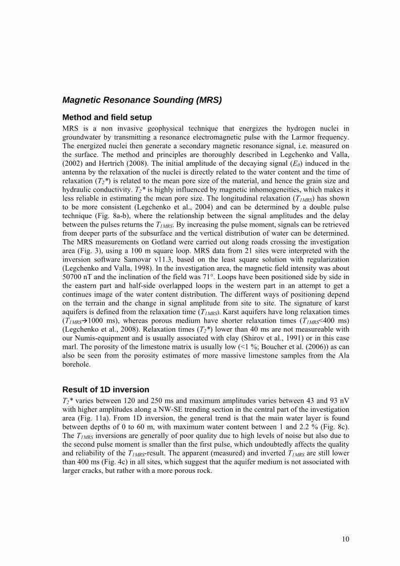
10
Magnetic Resonance Sounding (MRS)
Method and field setup MRS is a non invasive geophysical technique that energizes the hydrogen nuclei in groundwater by transmitting a resonance electromagnetic pulse with the Larmor frequency. The energized nuclei then generate a secondary magnetic resonance signal, i.e. measured on the surface. The method and principles are thoroughly described in Legchenko and Valla, (2002) and Hertrich (2008). The initial amplitude of the decaying signal (E0) induced in the antenna by the relaxation of the nuclei is directly related to the water content and the time of relaxation (T2*) is related to the mean pore size of the material, and hence the grain size and hydraulic conductivity. T2* is highly influenced by magnetic inhomogeneities, which makes it less reliable in estimating the mean pore size. The longitudinal relaxation (T1MRS) has shown to be more consistent (Legchenko et al., 2004) and can be determined by a double pulse technique (Fig. 8a-b), where the relationship between the signal amplitudes and the delay between the pulses returns the T1MRS. By increasing the pulse moment, signals can be retrieved from deeper parts of the subsurface and the vertical distribution of water can be determined. The MRS measurements on Gotland were carried out along roads crossing the investigation area (Fig. 3), using a 100 m square loop. MRS data from 21 sites were interpreted with the inversion software Samovar v11.3, based on the least square solution with regularization (Legchenko and Valla, 1998). In the investigation area, the magnetic field intensity was about 50700 nT and the inclination of the field was 71°. Loops have been positioned side by side in the eastern part and half-side overlapped loops in the western part in an attempt to get a continues image of the water content distribution. The different ways of positioning depend on the terrain and the change in signal amplitude from site to site. The signature of karst aquifers is defined from the relaxation time (T1MRS). Karst aquifers have long relaxation times (T1MRS 1000 ms), whereas porous medium have shorter relaxation times (T1MRS<400 ms) (Legchenko et al., 2008). Relaxation times (T2*) lower than 40 ms are not measureable with our Numis-equipment and is usually associated with clay (Shirov et al., 1991) or in this case marl. The porosity of the limestone matrix is usually low (<1 %; Boucher et al. (2006)) as can also be seen from the porosity estimates of more massive limestone samples from the Ala borehole.
Result of 1D inversion T2* varies between 120 and 250 ms and maximum amplitudes varies between 43 and 93 nV with higher amplitudes along a NW-SE trending section in the central part of the investigation area (Fig. 11a). From 1D inversion, the general trend is that the main water layer is found between depths of 0 to 60 m, with maximum water content between 1 and 2.2 % (Fig. 8c). The T1MRS inversions are generally of poor quality due to high levels of noise but also due to the second pulse moment is smaller than the first pulse, which undoubtedly affects the quality and reliability of the T1MRS-result. The apparent (measured) and inverted T1MRS are still lower than 400 ms (Fig. 4c) in all sites, which suggest that the aquifer medium is not associated with larger cracks, but rather with a more porous rock.
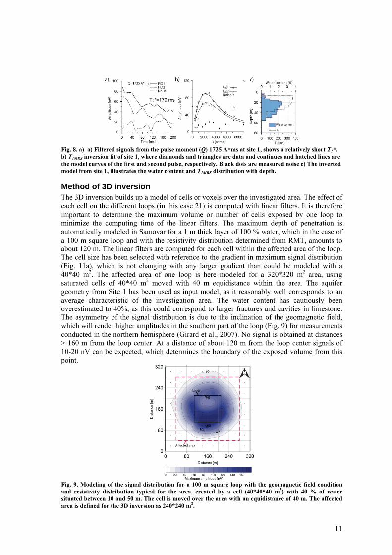
11
Fig. 8. a) a) Filtered signals from the pulse moment (Q) 1725 A*ms at site 1, shows a relatively short T2*.b) T1MRS inversion fit of site 1, where diamonds and triangles are data and continues and hatched lines are the model curves of the first and second pulse, respectively. Black dots are measured noise c) The inverted model from site 1, illustrates the water content and T1MRS distribution with depth.
Method of 3D inversion The 3D inversion builds up a model of cells or voxels over the investigated area. The effect of each cell on the different loops (in this case 21) is computed with linear filters. It is therefore important to determine the maximum volume or number of cells exposed by one loop to minimize the computing time of the linear filters. The maximum depth of penetration is automatically modeled in Samovar for a 1 m thick layer of 100 % water, which in the case of a 100 m square loop and with the resistivity distribution determined from RMT, amounts to about 120 m. The linear filters are computed for each cell within the affected area of the loop. The cell size has been selected with reference to the gradient in maximum signal distribution (Fig. 11a), which is not changing with any larger gradient than could be modeled with a 40*40 m2. The affected area of one loop is here modeled for a 320*320 m2 area, using saturated cells of 40*40 m2 moved with 40 m equidistance within the area. The aquifer geometry from Site 1 has been used as input model, as it reasonably well corresponds to an average characteristic of the investigation area. The water content has cautiously been overestimated to 40%, as this could correspond to larger fractures and cavities in limestone. The asymmetry of the signal distribution is due to the inclination of the geomagnetic field, which will render higher amplitudes in the southern part of the loop (Fig. 9) for measurements conducted in the northern hemisphere (Girard et al., 2007). No signal is obtained at distances > 160 m from the loop center. At a distance of about 120 m from the loop center signals of 10-20 nV can be expected, which determines the boundary of the exposed volume from this point.
Fig. 9. Modeling of the signal distribution for a 100 m square loop with the geomagnetic field condition and resistivity distribution typical for the area, created by a cell (40*40*40 m3) with 40 % of water situated between 10 and 50 m. The cell is moved over the area with an equidistance of 40 m. The affected area is defined for the 3D inversion as 240*240 m2.
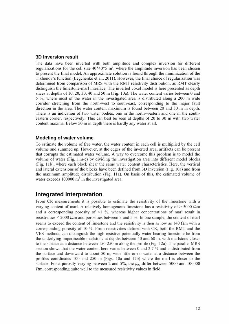
12
3D Inversion result The data have been inverted with both amplitude and complex inversion for different regularizations for the cell size 40*40*5 m3, where the amplitude inversion has been chosen to present the final model. An approximate solution is found through the minimization of the Tikhonov’s function (Legchenko et al., 2011). However, the final choice of regularization was determined from comparison of MRS with the RMT resistivity distribution, as RMT clearly distinguish the limestone-marl interface. The inverted voxel model is here presented as depth slices at depths of 10, 20, 30, 40 and 50 m (Fig. 10a). The water content varies between 0 and 5 %, where most of the water in the investigated area is distributed along a 200 m wide corridor stretching from the north-west to south-east, corresponding to the major fault direction in the area. The water content maximum is found between 20 and 30 m in depth. There is an indication of two water bodies, one in the north-western and one in the south-eastern corner, respectively. This can best be seen at depths of 20 to 30 m with two water content maxima. Below 50 m in depth there is hardly any water at all.
Modeling of water volume To estimate the volume of free water, the water content in each cell is multiplied by the cell volume and summed up. However, at the edges of the inverted area, artifacts can be present that corrupts the estimated water volume. A way to overcome this problem is to model the volume of water (Fig. 11a-c) by dividing the investigation area into different model blocks (Fig. 11b), where each block shear the same water content characteristics. Here, the vertical and lateral extensions of the blocks have been defined from 3D inversion (Fig. 10a) and from the maximum amplitude distribution (Fig. 11a). On basis of this, the estimated volume of water exceeds 100000 m3 in the investigated area.
Integrated Interpretation From CR measurements it is possible to estimate the resistivity of the limestone with a varying content of marl. A relatively homogenous limestone has a resistivity of > 5000 mand a corresponding porosity of <1 %, whereas higher concentrations of marl result in resistivities 2000 m and porosities between 3 and 5 %. In one sample, the content of marl seems to exceed the content of limestone and the resistivity is then as low as 140 m with a corresponding porosity of 10 %. From resistivities defined with CR, both the RMT and the VES methods can distinguish the high resistive potentially water bearing limestone be from the underlying impermeable marlstone at depths between 40 and 60 m, with marlstone closer to the surface at a distance between 150-250 m along the profile (Fig. 12a). The parallel MRS section shows that the water content here varies between 0 and 2.7 % and is distributed from the surface and downward to about 50 m, with little or no water at a distance between the profiles coordinates 100 and 250 m (Figs. 10a and 12b) where the marl is closer to the surface. For a porosity varying between 2 and 5%, the aq differ between 5000 and 100000
m, corresponding quite well to the measured resistivity values in field.
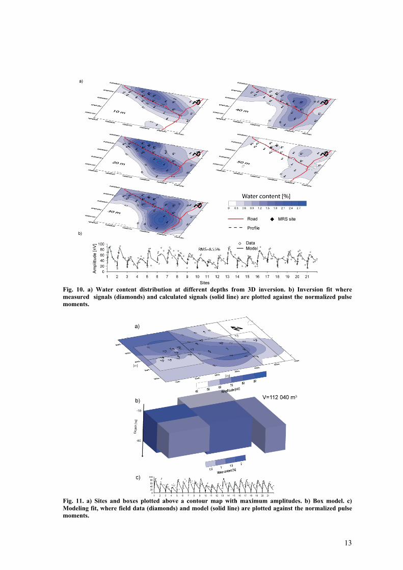
13
Fig. 10. a) Water content distribution at different depths from 3D inversion. b) Inversion fit where measured signals (diamonds) and calculated signals (solid line) are plotted against the normalized pulse moments.
Fig. 11. a) Sites and boxes plotted above a contour map with maximum amplitudes. b) Box model. c) Modeling fit, where field data (diamonds) and model (solid line) are plotted against the normalized pulse moments.
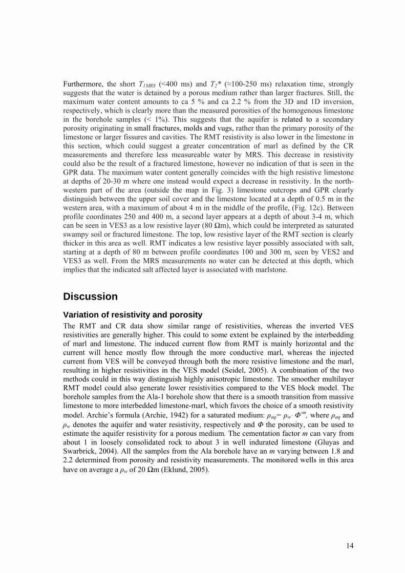
14
Furthermore, the short T1MRS (<400 ms) and T2* ( 100-250 ms) relaxation time, strongly suggests that the water is detained by a porous medium rather than larger fractures. Still, the maximum water content amounts to ca 5 % and ca 2.2 % from the 3D and 1D inversion, respectively, which is clearly more than the measured porosities of the homogenous limestone in the borehole samples (< 1%). This suggests that the aquifer is related to a secondary porosity originating in small fractures, molds and vugs, rather than the primary porosity of the limestone or larger fissures and cavities. The RMT resistivity is also lower in the limestone in this section, which could suggest a greater concentration of marl as defined by the CR measurements and therefore less measureable water by MRS. This decrease in resistivity could also be the result of a fractured limestone, however no indication of that is seen in the GPR data. The maximum water content generally coincides with the high resistive limestone at depths of 20-30 m where one instead would expect a decrease in resistivity. In the north-western part of the area (outside the map in Fig. 3) limestone outcrops and GPR clearly distinguish between the upper soil cover and the limestone located at a depth of 0.5 m in the western area, with a maximum of about 4 m in the middle of the profile, (Fig. 12c). Between profile coordinates 250 and 400 m, a second layer appears at a depth of about 3-4 m, which can be seen in VES3 as a low resistive layer (80 m), which could be interpreted as saturated swampy soil or fractured limestone. The top, low resistive layer of the RMT section is clearly thicker in this area as well. RMT indicates a low resistive layer possibly associated with salt, starting at a depth of 80 m between profile coordinates 100 and 300 m, seen by VES2 and VES3 as well. From the MRS measurements no water can be detected at this depth, which implies that the indicated salt affected layer is associated with marlstone.
Discussion Variation of resistivity and porosity The RMT and CR data show similar range of resistivities, whereas the inverted VES resistivities are generally higher. This could to some extent be explained by the interbedding of marl and limestone. The induced current flow from RMT is mainly horizontal and the current will hence mostly flow through the more conductive marl, whereas the injected current from VES will be conveyed through both the more resistive limestone and the marl, resulting in higher resistivities in the VES model (Seidel, 2005). A combination of the two methods could in this way distinguish highly anisotropic limestone. The smoother multilayer RMT model could also generate lower resistivities compared to the VES block model. The borehole samples from the Ala-1 borehole show that there is a smooth transition from massive limestone to more interbedded limestone-marl, which favors the choice of a smooth resistivity model. Archie’s formula (Archie, 1942) for a saturated medium: aq= w· -m, where aq and
w denotes the aquifer and water resistivity, respectively and the porosity, can be used to estimate the aquifer resistivity for a porous medium. The cementation factor m can vary from about 1 in loosely consolidated rock to about 3 in well indurated limestone (Gluyas and Swarbrick, 2004). All the samples from the Ala borehole have an m varying between 1.8 and 2.2 determined from porosity and resistivity measurements. The monitored wells in this area have on average a w of 20 m (Eklund, 2005).
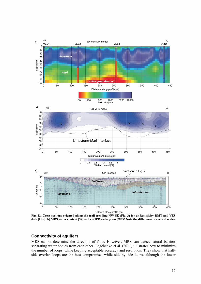
15
Fig. 12. Cross-sections oriented along the trail trending NW-SE (Fig. 3) for a) Resistivity RMT and VES data [ m]; b) MRS water content [%] and c) GPR radargram (OBS! Note the difference in vertical scale).
Connectivity of aquifers MRS cannot determine the direction of flow. However, MRS can detect natural barriers separating water bodies from each other. Legchenko et al. (2011) illustrates how to minimize the number of loops, while keeping acceptable accuracy and resolution. They show that half-side overlap loops are the best compromise, while side-by-side loops, although the lower
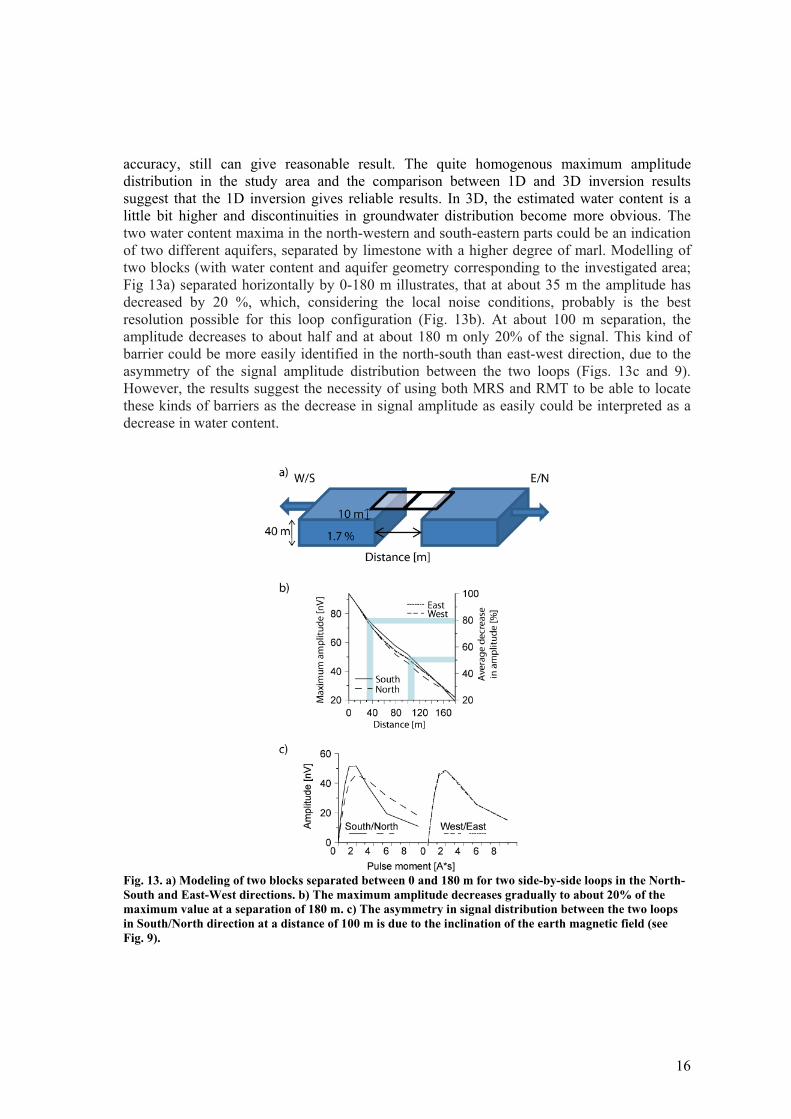
16
accuracy, still can give reasonable result. The quite homogenous maximum amplitude distribution in the study area and the comparison between 1D and 3D inversion results suggest that the 1D inversion gives reliable results. In 3D, the estimated water content is a little bit higher and discontinuities in groundwater distribution become more obvious. Thetwo water content maxima in the north-western and south-eastern parts could be an indication of two different aquifers, separated by limestone with a higher degree of marl. Modelling of two blocks (with water content and aquifer geometry corresponding to the investigated area; Fig 13a) separated horizontally by 0-180 m illustrates, that at about 35 m the amplitude has decreased by 20 %, which, considering the local noise conditions, probably is the best resolution possible for this loop configuration (Fig. 13b). At about 100 m separation, the amplitude decreases to about half and at about 180 m only 20% of the signal. This kind of barrier could be more easily identified in the north-south than east-west direction, due to the asymmetry of the signal amplitude distribution between the two loops (Figs. 13c and 9). However, the results suggest the necessity of using both MRS and RMT to be able to locate these kinds of barriers as the decrease in signal amplitude as easily could be interpreted as a decrease in water content.
Fig. 13. a) Modeling of two blocks separated between 0 and 180 m for two side-by-side loops in the North-South and East-West directions. b) The maximum amplitude decreases gradually to about 20% of the maximum value at a separation of 180 m. c) The asymmetry in signal distribution between the two loops in South/North direction at a distance of 100 m is due to the inclination of the earth magnetic field (see Fig. 9).
17
Conclusions In this study the geophysical methods MRS, RMT, VES and GPR were tested for characterizing aquifers in Gotland, in respect to geometry and storage as well as the connectivity of the aquifer over a more extensive area. The use of multiple techniques has shown to give a more coherent interpretation but also a more complete picture of the groundwater situation in the area. However, the shallow penetration depth of GPR and the lack of soil cover in some places of the investigated area make geoelectrical methods and GPR less efficient. MRS identifies the aquifer at depths between 10 and 60 m with maximum water contents at depths of 20 to 30 m. The water content varies between 0 and 5 % and relaxation times (T1MRS) less than 400 ms suggest that the aquifer medium consist of small fractures, molds and vugs rather than larger karst fractures and cavities. The boundaries between overburden, limestone and marl can be identified by RMT and VES. The peak water content measured with MRS usually coincides with the most resistive sections of the limestone, but no clear correlation can be seen between water content and resistivity. MRS is therefore the only method in this survey that actually detects water and thus determines the vertical and lateral distribution of water within the aquifer together with the free volume of water. Two potential aquifers were identified with MRS, possibly separated by marlstone. From modelling of two water saturated blocks it can be seen that a boundary between such two separated aquifer can be more easily discriminated in N/S-, than E/W direction due to the asymmetry of the signal distribution. RMT has shown to effectively characterize the limestone/marl interface but also to locate anomalous low resistive zones, possibly associated with salt water. RMT also helps to constrain the final MRS model by choosing a suitable regularization for the MRS 3D inversion. All together, the combination of MRS and RMT seems most efficient and promising for future groundwater explorations in geological environments like in Gotland.
Acknowledgement This study was funded by the foundation for technological and scientific research in memory of J. Gust. Richert (SWECO). Our deepest appreciation goes to Anatoly Legchenko for guidance of MRS 3D inversion and valuable advice in the interpretation of the MRS result. The authors acknowledge the Geological Survey of Sweden (SGU) for providing geological, geophysical and groundwater data from Gotland.
18
References Al-fares, W., Bakalowicz, M., Guerin, R. and Dukhan, M., 2002. Analysis of the karst aquifer
structure of the Lamalou area (Herault, France) with ground penetrating radar. JOURNAL OF APPLIED GEOPHYSICS, 51(2-4): 97-106.
Anchuela, O.P., Casas-Sainz, A.M., Soriano, M.A. and Pocovi-Juan, A., 2009. Mapping subsurface karst features with GPR: results and limitations. Environmental Geology, 58(2): 391-399.
Archie, G.E., 1942. The electrical resistivity log as an aid in determining some reservoir characteristics. Metallurgical and Petroleum Engineers 146: 54-62.
Bastani, M., 2001. EnviroMT- A New Controlled Source/Radio Magnetotelluric System Ph.D. Acta Universitatis Upsaliensis, Uppsala Dissertations from the Faculty of Science and Technology 32.
Boucher, M. et al., 2006. Using 2D inversion of magnetic resonance soundings to locate a water-filled karst conduit. JOURNAL OF HYDROLOGY, 330(3-4): 413-421.
Daniels, D.J., 2004. Ground Penetrating Radar Knoval (Institution of Engineering and Technology), London, 734 pp.
Eklund, F., 2005. Förändringar i grundvattenkvaliteten i 19 vattentäkter på Gotland under åren 1989-2004. Länsstyrelsen i Gotlands län, Visby, 133 pp.
Erlström, M., Persson, L., Sivhed, U. and Wickström, L., 2009. Beskrivning till regional berggrundskarta över Gotlands län. 978-91-7158-957-6, Sveriges geologiska undersökning, K221.
Girard, J.F., Boucher, M., Legchenko, A. and Baltassat, J.M., 2007. 2D magnetic resonance tomography applied to karstic conduit imaging. JOURNAL OF APPLIED GEOPHYSICS, 63(3-4): 103-116.
Gluyas, J. and Swarbrick, R.E., 2004. Petroleum geoscience. Blackwell publishing company, Oxford, UK, 361 pp.
Guerin, R. and Benderitter, Y., 1995. Shallow Karst Exploration Using Mt-Vlf and Dc Resistivity Methods. Geophysical Prospecting, 43(5): 635-653.
Hertrich, M., 2008. Imaging of groundwater with nuclear magnetic resonance. Progress in Nuclear Magnetic Resonance Spectroscopy, 53(4): 227-248.
Ismail, N., Schwarz, G. and Pedersen, L.B., 2011. Investigation of groundwater resources using controlled-source radio magnetotellurics (CSRMT) in glacial deposits in Heby, Sweden. JOURNAL OF APPLIED GEOPHYSICS, 73(1): 74-83.
Kalscheuer, T., Pedersen, L.B. and Siripunvaraporn, W., 2008. Radiomagnetotelluric two-dimensional forward and inverse modelling accounting for displacement currents. Geophysical Journal International, 175(2): 486-514.
Legchenko, A. et al., 2004. Magnetic resonance sounding applied to aquifer characterization. GROUND WATER, 42(3): 363-373.
Legchenko, A. et al., 2011. Three-dimensional magnetic resonance imaging for groundwater New Journal of Physics 13: 1-17.
19
Legchenko, A. et al., 2008. Locating water-filled karst caverns and estimating their volume using magnetic resonance soundings. GEOPHYSICS, 73(5): G51-G61.
Legchenko, A. and Valla, P., 1998. Processing of surface proton magnetic resonance signals using non-linear fitting. JOURNAL OF APPLIED GEOPHYSICS, 39(2): 77-83.
Legchenko, A. and Valla, P., 2002. A review of the basic principles for proton magnetic resonance sounding measurements. JOURNAL OF APPLIED GEOPHYSICS, 50(1-2): 3-19.
Linde, N. and Pedersen, L.B., 2004. Evidence of electrical anisotropy in limestone formations using the RMT technique. GEOPHYSICS, 69(4): 909-916.
Lindewald, H., 1985. Salt grundvatten i Sverige, rapporter och meddelanden. 39, Sveriges geologiska undersökning, Uppsala.
Lubczynski, M. and Roy, J., 2003. Hydrogeological interpretation and potential of the new magnetic resonance sounding (MRS) method. JOURNAL OF HYDROLOGY, 283(1-4): 19-40.
Olofsson, B., 1996. Salt Groundwater in Sweden - Occurence and Origin, Rapporter och meddelanden nr 87. In: SWIM (Editor), 14th Salt Water Intrusion Meeting. Geological Survey of Sweden, Malmö, Sweden, pp. 91-100.
Pedersen, L.B., Bastani, M. and Dynesius, L., 2005. Groundwater exploration using combined control led-source and radiomagnetotelluric techniques. GEOPHYSICS, 70(1): G8-G15.
Pedersen, L.B. and Engels, M., 2005. Routine 2D inversion of magnetotelluric data using the determinant of the impedance tensor. GEOPHYSICS, 70(2): G33-G41.
Pelton, W.H., Ward, S.H., Hallof, P.G., Sill, W.R. and Nelson, P.H., 1978. Mineral Discrimination and Removal of Inductive Coupling with Multifrequency-Ip. GEOPHYSICS, 43(3): 588-609.
Persson, L., Erlström, M., Bastani, M. and Pedersen, L.B., 2008. Airborne VLF measurement over the island of Gotland, Sweden, Extended abstract AEM2008, 5th International Conference on Airborne Electromagnetics, Haikko Manor, Finland, pp. 28-30.
Seidel, K., 2005. Elektromagnetische Zweispulen-Systeme, Prinzip der Methode. In: K.K. Knödel K, Lange G (Editor), Handbuch zur Erkundung des Untergrundes von Deponien und Altlasten. Springer, Berlin Heidelberg NewYork.
SEPA, 2007. Environmental quality criteria for groundwater, Swedish Environmental Protection Agency (SEPA).
Shirov, M., Legchenko, A. and Creer, G., 1991. A new direct non-invasive groundwater detection technology for Australia. Exploration Geophysics 22: 333-338.
Siripunvaraporn, W. and Egbert, G., 2000. An efficient data-subspace inversion method for 2-D magnetotelluric data. GEOPHYSICS, 65(3): 791-803.
Triumf, C.-A., Thunehed, H. and Antal, I., 2000. Bestämning av elektriska egenskaper hos vulkaniter från Skellefte- och Arvidsjaurgrupperna. Sveriges geologiska undersökning 2000:8: 30 pp.
Turberg, P., 1994. Hydrogeological investigation of porous environments by radio magnetotelluric-resistivity (RMT-R 12-240 kHz). JOURNAL OF APPLIED GEOPHYSICS, 31(1-4): 133.

20
Vattenmyndigheten, 2007. Miljöövervakning av vatten - tillstånd hos inlands-, kust- och grundvatten i Södra Östersjöns vattendistrikt, Kalmar, 186 pp.
Vouillamoz, J.M. et al., 2003. Localization of saturated karst aquifer with magnetic resonance sounding and resistivity imagery. GROUND WATER, 41(5): 578-586.
Paper IV
Field evaluation of the MRS Spin-Echo method under geological conditions typical for the northern part of Sweden
Perttu, N., Legchenko, A., Vouillamoz, J.M. and Elming, S-Å (2011) Submitted to Journal of Applied Geophysics

1
Field evaluation of the MRS Spin-Echo method under geological conditions typical for the northern Sweden N. Perttua,*, A. Legchenkob, J.M. Vouillamozb, S-Å. Elminga aDivision of Geosciences, Luleå University of Technology, SE-971 87 Luleå, Sweden bIRD/ UJF-Grenoble 1/CNRS/G-INP, LTHE UMR 5564, Grenoble F-38041, France *Corresponding author. Tel.: +46 920 491884; fax: +46 920 491199. E-mail address: [email protected] (N. Perttu).
AbstractThe Magnetic Resonance Sounding (MRS) method, unlike other geophysical techniques, is directly sensitive to the water content in the ground and could contribute in characterization of aquifers in Sweden. However, standard MRS measurements have so far been unsuccessful in detecting water in the northern part of Sweden. This is due to large magnetic gradients caused by the crystalline basement rock, high magnetic susceptibility of the soils and electromagnetic noise in or in proximity to urbanized areas. In this study, the recently implemented MRS spin echo (SE) technique has been applied on ice roads in the Bothnian bay (Baltic Sea) to test the reliability of MRS SE results and the influence of large scale magnetic gradients on the MRS signals. The MRS SE technique has further been tested for different soil types in and in proximity to groundwater supplies in the city of Luleå, where the result has been compared and evaluated with geophysical and geological data. The measuring procedure has subsequently been tested and optimized to meet the conditions of magnetic environments. MRS SE measurements have shown to give reliable results from measurements on ice over free water, although, T2MRS are clearly affected by diffusion due to the long extrapolation time. From Earth magnetic field variations over the loop, it is noticed that even small horizontal intensity gradients in the field affect the T2* and that larger gradients > 100 nT/’affected area of the loop’ can diminish the T2* from 1000 ms to < 50 ms. The two separated square loop configuration used for measurements on land has shown to be very flexible in terms of location of the two squares compared to the figure eight loop but also efficient in reducing noise by careful adjustment of the loop layout. Measurements made in different geological environments show that the MRS SE technique cannot detect water in finer tills, silt and clays, constrained by the minimum delay time of the instrument (ca 70 ms), but is more suitable in coarser soils such as sand and gravel deposits. The MRS SE result from the site of the Luleå town water supply shows a good agreement with the estimated effective porosity from a near by borehole. Complementary GPR measurements have shown to be very efficient in characterizing the aquifer in respect to the groundwater table, layering and sediment structures. No free induction decay (FID) signals were observed in MRS records in measurement made on land, which decreases the risk of mixing FID and SE signals. Therefore, a standard SE measuring procedure (q2=2q1) is most successful with a pulse duration of 15 ms (q1).
2
IntroductionSweden’s favorable climate (on average 554 mm of rain/year) and the eligible geology, in particular the many sand and gravel deposits, create perfect reservoirs for clean and easy accessible drinking water. About 50 % of the drinking water in Sweden originates naturally from groundwater or from “artificial groundwater”, i.e. water from rivers, lakes and creeks, filtered through sand or gravel deposits. The groundwater from municipal drinking water sources in Sweden is generally considered to be of good quality. However, in a nationwide survey of groundwater quality of private wells (Socialstyrelsen, 2008), the water in as much as 10 % of the drilled wells and 35 % of the dug wells in the study were declared unfit for human consumption. The main problems were related to microbiological growth, and elevated concentration of nutrients, salt, arsenic and uranium. Some of the major threats to Swedish drinking water resources are: the depletion of natural gravel deposits from quarrying, pollution from industrial activities, transportation and construction, and excessive withdrawal of groundwater in coastal areas leading to saltwater intrusion (SGU, 2011). The challenges of future groundwater planning and management according to SGU are on the determination of (1) where potential groundwater reservoirs are seated and the assessment of their capacity to provide sufficient and clean water on a yearly basis; (2) where lake or river water can be treated naturally by artificial infiltration and (3) where water can be obtained if a regular source for some reason has been contaminated or in other respects unfit to be used. Soil-, bedrock- and groundwater maps provide information about the locality of potential aquifers, however, little is known about vertical extension, layering, homogeneity, yield, porosity or transmissivity. Magnetic Resonance Sounding method (MRS) is a relatively new, non invasive method that in contrast to all other geophysical techniques is directly sensitive to the water content in the ground (Hertrich, 2008; Legchenko and Valla, 2002; Shirov et al., 1991). MRS has also proven to be a very promising tool in estimating storage and hydraulic parameters in fractured and weathered non-magnetic hard rocks (Baltassat et al., 2005; Descloitres et al., 2008; Legchenko et al., 2008; Lubczynski and Roy, 2005; Roy and Lubczynski, 2003). Due to large magnetic gradients caused by the crystalline basement rock, high magnetic susceptibility of the soils and high electromagnetic noise in or in proximity to urbanized areas, MRS measurements have until recently been unsuccessful in detecting water in the northern part of Sweden (Wattanasen and Elming, 2008). Problems related to high magnetic gradients resulting in poor MRS signals or unreliable data have been reported from other parts of the world as well (Legchenko et al., 2002; Roy et al., 2008). Recently, the more intricate MRS Spin Echo (SE) technique (Hahn, 1950) has been implemented in magnetic environments, such as Canada, Cyprus and India (Legchenko et al., 2010; Vouillamoz et al., 2011) and it has proven successful in detecting water where standard MRS measuring procedures earlier were unsuccessful. In this study, standard- and SE measurements have been conducted on ice roads in the Bothnian bay, situated in the very northern part of the Baltic Sea (Fig. 1a). The area offers a good environment to test the reliability of MRS SE result and the influence of large scale magnetic gradients on the MRS signals. The MRS SE technique has also been tested in different soil types in and in proximity to the main groundwater supplies of the city of Luleå, where the result was compared and evaluated with geophysical and existing geological data. The measuring procedure has subsequently been optimized to meet the conditions of magnetic environments.
3
Geological setting The investigated area is part of the Fennoscandian shield and consists of intrusive, volcanic, metamorphic and sedimentary rocks, mostly of 1.9-1.8 Ga ages (SGU, 2009). In parts of the study area, geological maps are lacking. Still, large positive magnetic anomalies can normally be associated with intrusive gabbros, whereas smaller positive anomalies are associated with granitoids. Low magnetic field intensities are usually associated with meta-sedimentary rocks such as meta-greywacke in the eastern part of the area. The largest magnetic gradients are found in the area of Hindersön and Kvarnträskholmen (Fig. 1b). Larger fracture zones are present in the western part of the study area (Fig. 1b), trending in northwest-southeast directions and associated with magnetic field minima. The area is to a large extent covered with glacial till but glacial and post glacial sand deposits are common within the investigated area as well as finer sediments as clay and silt. The average depth to the bed rock is 15 m, but varies from 0 to 64 m. Soils with high aquifer potential are usually associated with coarser sediments, such as sand and gravel (producing 5-25 l/s) and constitutes less than 3.5 % of the investigated area, whereas potential rock aquifers (0.2-0.6 l/s) are usually associated with high fracture density. The magnetic susceptibilities of the rocks from outcrops (SGU, 2009) varies on average between 10-3 to 10-2 SI with same range of values for soft sediments like sand and till, but somewhat smaller values for more clayey soils.
The MRS Spin-Echo (SE) Method The MRS SE method is a large-scale geophysical implementation of the spin-echo technique developed by Hahn in 1950 for measuring Nuclear Magnetic Resonance (NMR) response in a non homogenous static magnetic field (Hahn, 1950). The hydrogen nuclei in water have magnetic moments, as they can be seen as charged particles spinning in the Larmor frequency ( L). The net magnetization (M0) of the nuclei (1) will be oriented along the Earth magnetic field (B0) (Fig. 2a (1)). In the MRS technique a coincident transmitting-receiving loop is used to transmit a pulse moment (q1) of alternating current in the Larmor frequency ( L) (Fig. 2b(2)). This will deflect the magnetization vector 90° into the x-y plane. After the pulse is turned off, the instrument turn into receiving mode during a dead time of 40 ms. The nuclei return to their equilibrium position, while creating a relaxation magnetic field measured in the same loop on the surface, where the initial amplitude of the field is proportional to the amount of water within the investigated volume. Due to magnetic inhomogeneities, the individual magnetic moments are spinning at different rates, some faster and some slower (Fig. 2a-b (2)), dispersing the relaxation magnetic field and shortening the relaxation time (T2*) of the signal. Free induction decay (FID) signals with T2* shorter than 40 ms are not measureable with current Numis equipment. After a period of time ( e), a second pulse moment (q2=2·q1) with a flip angle ( ) of 180° ( 2=2· 1) turns the spins over to the other side of the x-y plane (Fig. 2a-b (3)). The nuclei with higher Larmor frequencies are now behind whereas the nuclei with lower Larmor frequencies are ahead. At the time of e after the second pulse all the spins are once again in phase creating a rise in the relaxation field signal (Fig. 2a-b (4)) that under near resonance conditions can be calculated as M =-M0·sin( 1) · sin2( 1) (Bloom, 1955), where the amplitude of the SE signal (e2 ) at time 2· e after the first pulse is
MRS
e
TSEe
202
2exp (1)
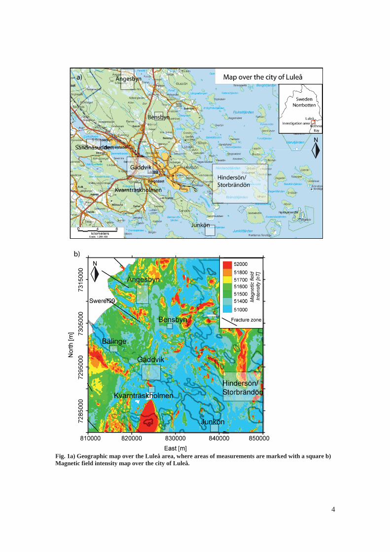
4
Fig. 1a) Geographic map over the Luleå area, where areas of measurements are marked with a square b) Magnetic field intensity map over the city of Luleå.
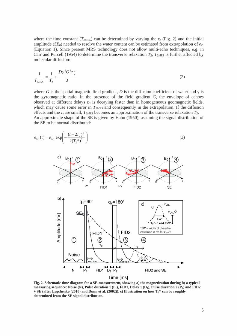
5
where the time constant (T2MRS) can be determined by varying the e (Fig. 2) and the initial amplitude (SE0) needed to resolve the water content can be estimated from extrapolation of e2 (Equation 1). Since present MRS technology does not allow multi-echo techniques, e.g. in Carr and Purcell (1954) to determine the transverse relaxation T2, T2MRS is further affected by molecular diffusion:
311
222
22
e
MRS
GD
TT (2)
where G is the spatial magnetic field gradient, D is the diffusion coefficient of water and is the gyromagnetic ratio. In the presence of the field gradient G, the envelope of echoes observed at different delays ei is decaying faster than in homogeneous geomagnetic fields, which may cause some error in T2MRS and consequently in the extrapolation. If the diffusion effects and the e are small, T2MRS becomes an approximation of the transverse relaxation T2. An approximate shape of the SE is given by Hahn (1950), assuming the signal distribution of the SE to be normal distributed:
22
2
2 *)(2)2(exp)(
Ttete e
SE e (3)
Fig. 2. Schematic time diagram for a SE-measurement, showing a) the magnetization during b) a typical measuring sequence: Noise (N), Pulse duration 1 (P1), FID1, Delay 1 (D1), Pulse duration 2 (P2) and FID2 + SE (after Legchenko (2010) and Dunn et al. (2002)). c) Illustration on how T2* can be roughly determined from the SE signal distribution.
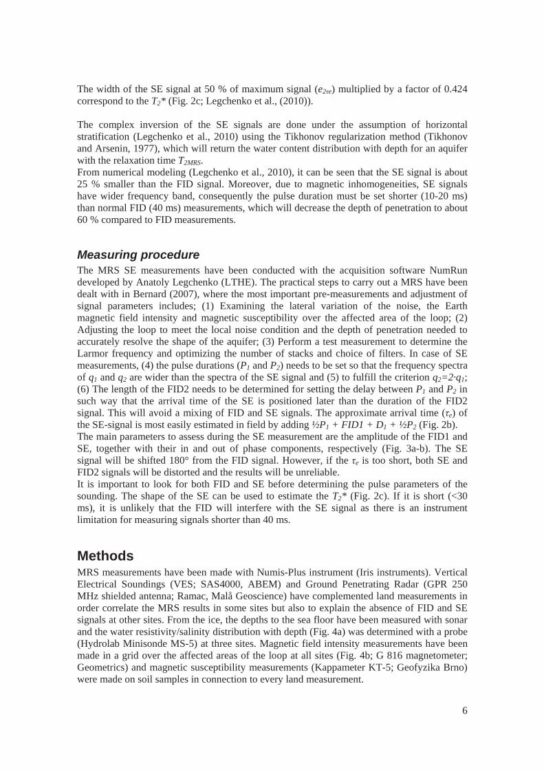
6
The width of the SE signal at 50 % of maximum signal (e2 e) multiplied by a factor of 0.424 correspond to the T2* (Fig. 2c; Legchenko et al., (2010)). The complex inversion of the SE signals are done under the assumption of horizontal stratification (Legchenko et al., 2010) using the Tikhonov regularization method (Tikhonov and Arsenin, 1977), which will return the water content distribution with depth for an aquifer with the relaxation time T2MRS. From numerical modeling (Legchenko et al., 2010), it can be seen that the SE signal is about 25 % smaller than the FID signal. Moreover, due to magnetic inhomogeneities, SE signals have wider frequency band, consequently the pulse duration must be set shorter (10-20 ms) than normal FID (40 ms) measurements, which will decrease the depth of penetration to about 60 % compared to FID measurements.
Measuring procedure The MRS SE measurements have been conducted with the acquisition software NumRun developed by Anatoly Legchenko (LTHE). The practical steps to carry out a MRS have been dealt with in Bernard (2007), where the most important pre-measurements and adjustment of signal parameters includes; (1) Examining the lateral variation of the noise, the Earth magnetic field intensity and magnetic susceptibility over the affected area of the loop; (2) Adjusting the loop to meet the local noise condition and the depth of penetration needed to accurately resolve the shape of the aquifer; (3) Perform a test measurement to determine the Larmor frequency and optimizing the number of stacks and choice of filters. In case of SE measurements, (4) the pulse durations (P1 and P2) needs to be set so that the frequency spectra of q1 and q2 are wider than the spectra of the SE signal and (5) to fulfill the criterion q2=2·q1; (6) The length of the FID2 needs to be determined for setting the delay between P1 and P2 in such way that the arrival time of the SE is positioned later than the duration of the FID2 signal. This will avoid a mixing of FID and SE signals. The approximate arrival time ( e) of the SE-signal is most easily estimated in field by adding ½P1 + FID1 + D1 + ½P2 (Fig. 2b). The main parameters to assess during the SE measurement are the amplitude of the FID1 and SE, together with their in and out of phase components, respectively (Fig. 3a-b). The SE signal will be shifted 180° from the FID signal. However, if the e is too short, both SE and FID2 signals will be distorted and the results will be unreliable. It is important to look for both FID and SE before determining the pulse parameters of the sounding. The shape of the SE can be used to estimate the T2* (Fig. 2c). If it is short (<30 ms), it is unlikely that the FID will interfere with the SE signal as there is an instrument limitation for measuring signals shorter than 40 ms.
MethodsMRS measurements have been made with Numis-Plus instrument (Iris instruments). Vertical Electrical Soundings (VES; SAS4000, ABEM) and Ground Penetrating Radar (GPR 250 MHz shielded antenna; Ramac, Malå Geoscience) have complemented land measurements in order correlate the MRS results in some sites but also to explain the absence of FID and SE signals at other sites. From the ice, the depths to the sea floor have been measured with sonar and the water resistivity/salinity distribution with depth (Fig. 4a) was determined with a probe (Hydrolab Minisonde MS-5) at three sites. Magnetic field intensity measurements have been made in a grid over the affected areas of the loop at all sites (Fig. 4b; G 816 magnetometer; Geometrics) and magnetic susceptibility measurements (Kappameter KT-5; Geofyzika Brno) were made on soil samples in connection to every land measurement.
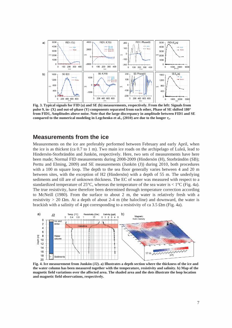
7
Fig. 3. Typical signals for FID (a) and SE (b) measurements, respectively. From the left: Signals from pulse 9, in- (X) and out-of-phase (Y) components separated from each other, Phase of SE shifted 180° from FID1, Amplitudes above noise. Note that the large discrepancy in amplitude between FID1 and SE compared to the numerical modeling in Legchenko et al., (2010) are due to the longer e.
Measurements from the ice Measurements on the ice are preferably performed between February and early April, when the ice is as thickest (ca 0.7 to 1 m). Two main ice roads on the archipelago of Luleå, lead to Hindersön-Storbrändön and Junkön, respectively. Here, two sets of measurements have here been made; Normal FID measurements during 2008-2009 (Hindersön (H), Storbrändön (SB); Perttu and Elming, 2009) and SE measurements (Junkön (J)) during 2010, both procedures with a 100 m square loop. The depth to the sea floor generally varies between 4 and 20 m between sites, with the exception of H2 (Hindersön) with a depth of 55 m. The underlying sediments and till are of unknown thickness. The EC of water was measured with respect to a standardized temperature of 25°C, whereas the temperature of the sea water is < 1°C (Fig. 4a). The true resistivity, have therefore been determined through temperature correction according to McNeill (1980). From the surface to about 2 m, the water is relatively fresh with a resistivity > 20 m. At a depth of about 2-4 m (the halocline) and downward, the water is brackish with a salinity of 4 ppt corresponding to a resistivity of ca 3.5 m (Fig. 4a).
Fig. 4. Ice measurement from Junkön (J2). a) Illustrates a depth section where the thickness of the ice and the water column has been measured together with the temperature, resistivity and salinity. b) Map of the magnetic field variations over the affected area. The shaded area and the dots illustrate the loop location and magnetic field observations, respectively.
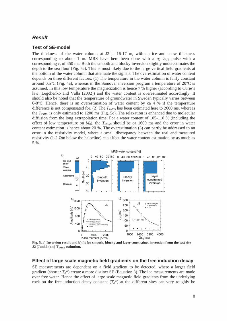
8
Result
Test of SE-model The thickness of the water column at J2 is 16-17 m, with an ice and snow thickness corresponding to about 1 m. MRS have here been done with a q2=2q1 pulse with a corresponding e of 450 ms. Both the smooth and blocky inversion slightly underestimates the depth to the sea floor (Fig. 5a). This is most likely due to the large vertical field gradients at the bottom of the water column that attenuate the signals. The overestimation of water content depends on three different factors; (1) The temperature in the water column is fairly constant around 0.5°C (Fig. 4a), whereas in the Samovar inversion program a temperature of 20°C is assumed. In this low temperature the magnetization is hence 7 % higher (according to Curie’s law; Legchenko and Valla (2002)) and the water content is overestimated accordingly. It should also be noted that the temperature of groundwater in Sweden typically varies between 6-8°C. Hence, there is an overestimation of water content by ca 4 % if the temperature difference is not compensated for. (2) The T1MRS has been estimated here to 2600 ms, whereas the T2MRS is only estimated to 1200 ms (Fig. 5c). The relaxation is enhanced due to molecular diffusion from the long extrapolation time. For a water content of 105-110 % (including the effect of low temperature on M0), the T2MRS should be ca 1600 ms and the error in water content estimation is hence about 20 %. The overestimation (3) can partly be addressed to an error in the resistivity model, where a small discrepancy between the real and measured resistivity (1-2 m below the halocline) can affect the water content estimation by as much as 5 %.
Fig. 5. a) Inversion result and b) fit for smooth, blocky and layer constrained inversion from the test site J2 (Junkön). c) T2MRS estimtion.
Effect of large scale magnetic field gradients on the free induction decaySE measurements are dependent on a field gradient to be detected, where a larger field gradient (shorter T2*) create a more distinct SE (Equation 3). The ice measurements are made over free water. Hence the effect of large scale magnetic field gradients from the underlying rock on the free induction decay constant (T2*) at the different sites can very roughly be
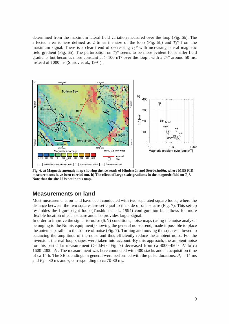
9
determined from the maximum lateral field variation measured over the loop (Fig. 6b). The affected area is here defined as 2 times the size of the loop (Fig. 5b) and T2* from the maximum signal. There is a clear trend of decreasing T2* with increasing lateral magnetic field gradient (Fig. 6b). The perturbation on T2* seems to be more evident for smaller field gradients but becomes more constant at > 100 nT/’over the loop’, with a T2* around 50 ms, instead of 1000 ms (Shirov et al., 1991).
Fig. 6. a) Magnetic anomaly map showing the ice roads of Hindersön and Storbrändön, where MRS FID measurements have been carried out. b) The effect of large scale gradients in the magnetic field on T2*.Note that the site J2 is not in this map.
Measurements on land Most measurements on land have been conducted with two separated square loops, where the distance between the two squares are set equal to the side of one square (Fig. 7). This set-up resembles the figure eight loop (Trushkin et al., 1994) configuration but allows for more flexible location of each square and also provides larger signal. In order to improve the signal-to-noise (S/N) conditions, noise maps (using the noise analyzer belonging to the Numis equipment) showing the general noise trend, made it possible to place the antenna parallel to the source of noise (Fig. 7). Turning and moving the squares allowed to balancing the amplitude of the noise and thus efficiently reduce the ambient noise. For the inversion, the real loop shapes were taken into account. By this approach, the ambient noise for this particular measurement (Gäddvik; Fig. 7) decreased from ca 4000-4500 nV to ca 1600-2000 nV. The measurement was here conducted with 400 stacks and an acquisition time of ca 14 h. The SE soundings in general were performed with the pulse durations: P1 = 14 ms and P2 = 30 ms and e corresponding to ca 70-80 ms.
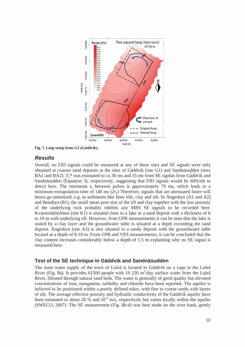
10
Fig. 7. Loop setup from G1 (Gäddvik).
Results Overall, no FID signals could be measured at any of these sites and SE signals were only obtained at coarser sand deposits at the sites of Gäddvik (site G1) and Sandnäsudden (sites BA1 and BA2). T2* was estimated to ca 30 ms and 35 ms from SE signlas from Gäddvik and Sandnäsudden (Equation 3), respectively, suggesting that FID signals would be difficult to detect here. The minimum e between pulses is approximately 70 ms, which leads to a minimum extrapolation time of 140 ms (2 e) Therefore, signals that are attenuated faster will hence go unnoticed, e.g. in sediments like finer tills, clay and silt. In Ängesbyn (A1 and A2) and Bensbyn (B1), the small mean pore size of the till and clay together with the low porosity of the underlying rock probably inhibits any MRS SE signals to be recorded here. Kvarnträskholmen (site K1) is situated close to a lake in a sand deposit with a thickness of 6 to 10 m with underlying till. However, from GPR measurements it can be seen that the lake is sealed by a clay layer and the groundwater table is situated at a depth exceeding the sand deposit. Ängesbyn (site A3) is also situated in a sandy deposit with the groundwater table located at a depth of 8-10 m. From GPR and VES measurements, it can be concluded that the clay content increases considerably below a depth of 1.5 m explaining why no SE signal is measured here.
Test of the SE technique in Gäddvik and Sandnäsudden The main water supply of the town of Luleå is located in Gäddvik on a cape in the Luleå River (Fig. 8a). It provides 61500 people with 19 250 m3/day surface water from the Luleå River, filtrated through natural sand beds. The water is generally of good quality but elevated concentrations of iron, manganese, turbidity and chloride have been reported. The aquifer is believed to be positioned within a poorly defined esker, with fine to coarse sands with layers of silt. The average effective porosity and hydraulic conductivity of the Gäddvik aquifer have been estimated to about 20 % and 10-3 m/s, respectively but varies locally within the aquifer (SWECO, 2007). The SE measurement (Fig. 8b-d) was here made on the river bank, gently
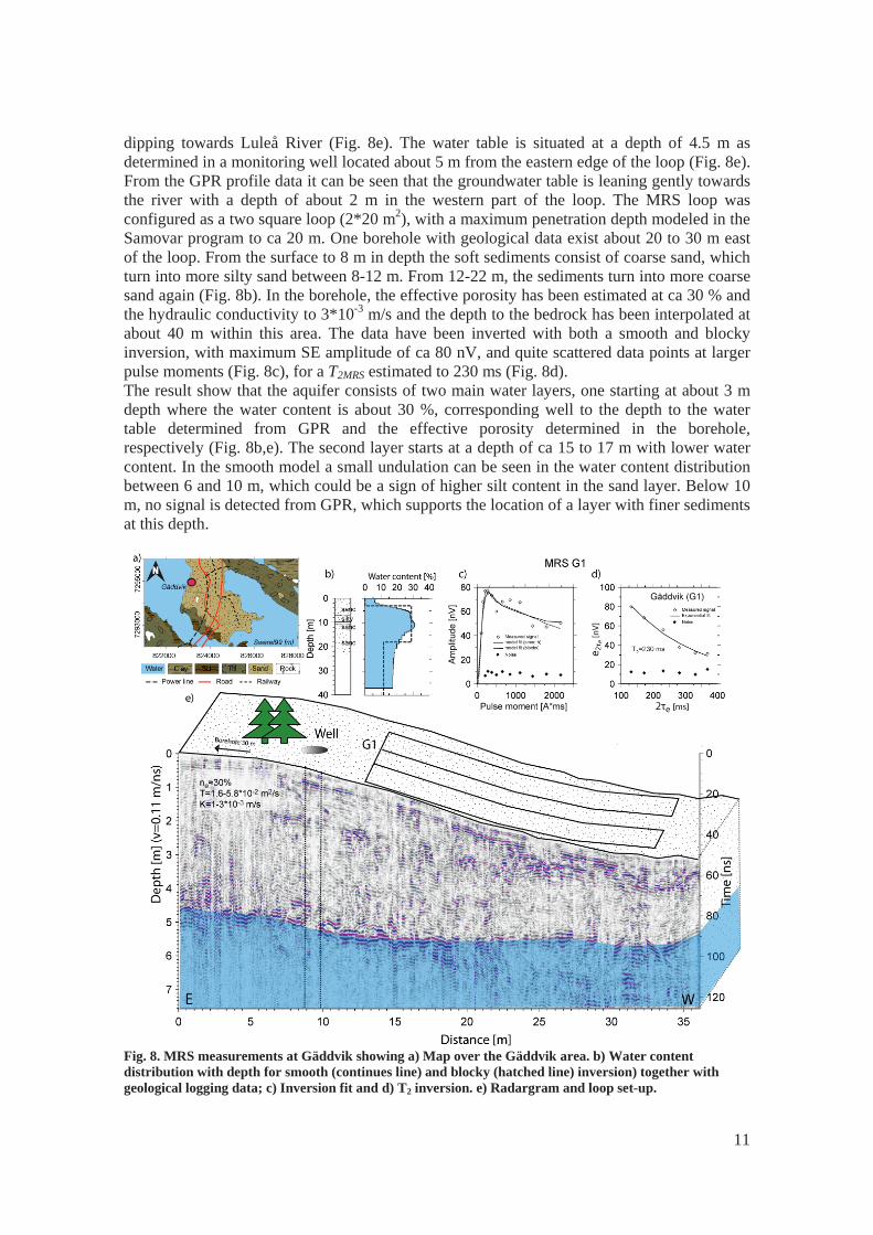
11
dipping towards Luleå River (Fig. 8e). The water table is situated at a depth of 4.5 m as determined in a monitoring well located about 5 m from the eastern edge of the loop (Fig. 8e). From the GPR profile data it can be seen that the groundwater table is leaning gently towards the river with a depth of about 2 m in the western part of the loop. The MRS loop was configured as a two square loop (2*20 m2), with a maximum penetration depth modeled in the Samovar program to ca 20 m. One borehole with geological data exist about 20 to 30 m east of the loop. From the surface to 8 m in depth the soft sediments consist of coarse sand, which turn into more silty sand between 8-12 m. From 12-22 m, the sediments turn into more coarse sand again (Fig. 8b). In the borehole, the effective porosity has been estimated at ca 30 % and the hydraulic conductivity to 3*10-3 m/s and the depth to the bedrock has been interpolated at about 40 m within this area. The data have been inverted with both a smooth and blocky inversion, with maximum SE amplitude of ca 80 nV, and quite scattered data points at larger pulse moments (Fig. 8c), for a T2MRS estimated to 230 ms (Fig. 8d). The result show that the aquifer consists of two main water layers, one starting at about 3 m depth where the water content is about 30 %, corresponding well to the depth to the water table determined from GPR and the effective porosity determined in the borehole, respectively (Fig. 8b,e). The second layer starts at a depth of ca 15 to 17 m with lower water content. In the smooth model a small undulation can be seen in the water content distribution between 6 and 10 m, which could be a sign of higher silt content in the sand layer. Below 10 m, no signal is detected from GPR, which supports the location of a layer with finer sediments at this depth.
Fig. 8. MRS measurements at Gäddvik showing a) Map over the Gäddvik area. b) Water content distribution with depth for smooth (continues line) and blocky (hatched line) inversion) together with geological logging data; c) Inversion fit and d) T2 inversion. e) Radargram and loop set-up.
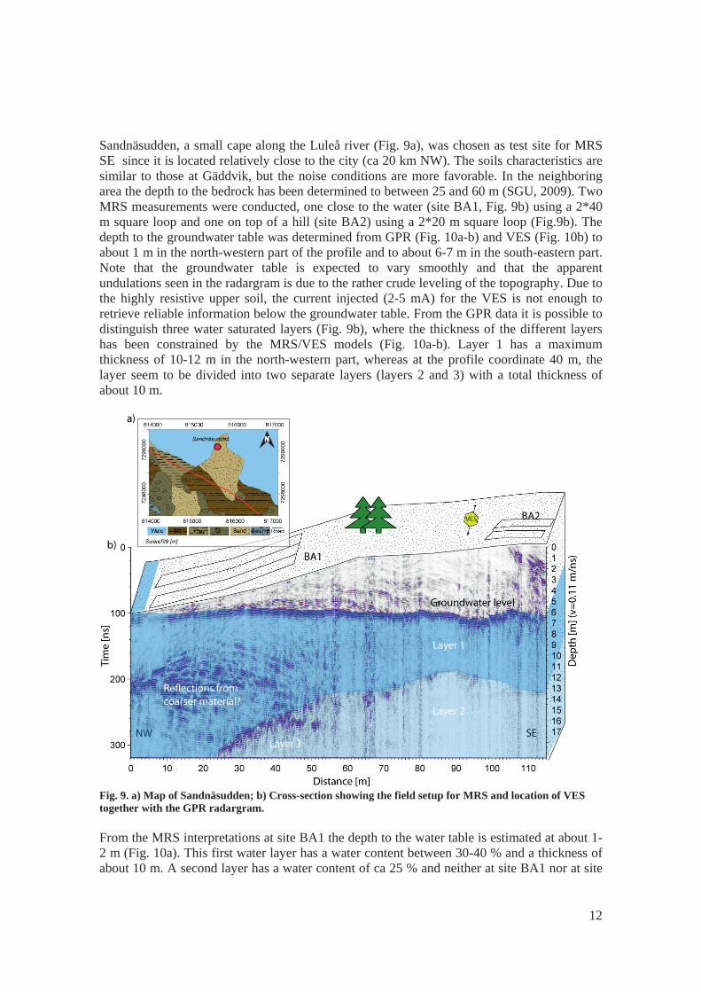
12
Sandnäsudden, a small cape along the Luleå river (Fig. 9a), was chosen as test site for MRS SE since it is located relatively close to the city (ca 20 km NW). The soils characteristics are similar to those at Gäddvik, but the noise conditions are more favorable. In the neighboring area the depth to the bedrock has been determined to between 25 and 60 m (SGU, 2009). Two MRS measurements were conducted, one close to the water (site BA1, Fig. 9b) using a 2*40 m square loop and one on top of a hill (site BA2) using a 2*20 m square loop (Fig.9b). The depth to the groundwater table was determined from GPR (Fig. 10a-b) and VES (Fig. 10b) to about 1 m in the north-western part of the profile and to about 6-7 m in the south-eastern part. Note that the groundwater table is expected to vary smoothly and that the apparent undulations seen in the radargram is due to the rather crude leveling of the topography. Due to the highly resistive upper soil, the current injected (2-5 mA) for the VES is not enough to retrieve reliable information below the groundwater table. From the GPR data it is possible to distinguish three water saturated layers (Fig. 9b), where the thickness of the different layers has been constrained by the MRS/VES models (Fig. 10a-b). Layer 1 has a maximum thickness of 10-12 m in the north-western part, whereas at the profile coordinate 40 m, the layer seem to be divided into two separate layers (layers 2 and 3) with a total thickness of about 10 m.
Fig. 9. a) Map of Sandnäsudden; b) Cross-section showing the field setup for MRS and location of VES together with the GPR radargram. From the MRS interpretations at site BA1 the depth to the water table is estimated at about 1-2 m (Fig. 10a). This first water layer has a water content between 30-40 % and a thickness of about 10 m. A second layer has a water content of ca 25 % and neither at site BA1 nor at site
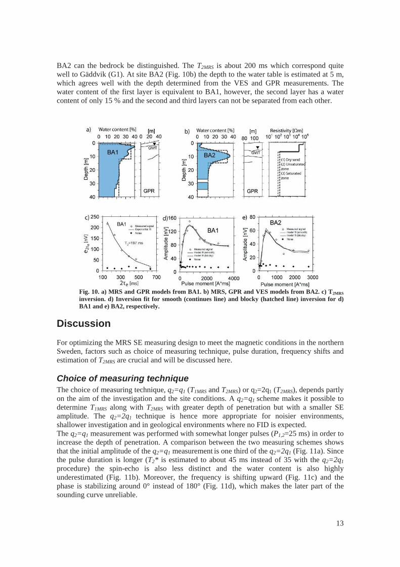
13
BA2 can the bedrock be distinguished. The T2MRS is about 200 ms which correspond quite well to Gäddvik (G1). At site BA2 (Fig. 10b) the depth to the water table is estimated at 5 m, which agrees well with the depth determined from the VES and GPR measurements. The water content of the first layer is equivalent to BA1, however, the second layer has a water content of only 15 % and the second and third layers can not be separated from each other.
Fig. 10. a) MRS and GPR models from BA1. b) MRS, GPR and VES models from BA2. c) T2MRSinversion. d) Inversion fit for smooth (continues line) and blocky (hatched line) inversion for d) BA1 and e) BA2, respectively.
Discussion
For optimizing the MRS SE measuring design to meet the magnetic conditions in the northern Sweden, factors such as choice of measuring technique, pulse duration, frequency shifts and estimation of T2MRS are crucial and will be discussed here.
Choice of measuring technique The choice of measuring technique, q2=q1 (T1MRS and T2MRS) or q2=2q1 (T2MRS), depends partly on the aim of the investigation and the site conditions. A q2=q1 scheme makes it possible to determine T1MRS along with T2MRS with greater depth of penetration but with a smaller SE amplitude. The q2=2q1 technique is hence more appropriate for noisier environments, shallower investigation and in geological environments where no FID is expected. The q2=q1 measurement was performed with somewhat longer pulses (P1,2=25 ms) in order to increase the depth of penetration. A comparison between the two measuring schemes shows that the initial amplitude of the q2=q1 measurement is one third of the q2=2q1 (Fig. 11a). Since the pulse duration is longer (T2* is estimated to about 45 ms instead of 35 with the q2=2q1 procedure) the spin-echo is also less distinct and the water content is also highly underestimated (Fig. 11b). Moreover, the frequency is shifting upward (Fig. 11c) and the phase is stabilizing around 0° instead of 180° (Fig. 11d), which makes the later part of the sounding curve unreliable.
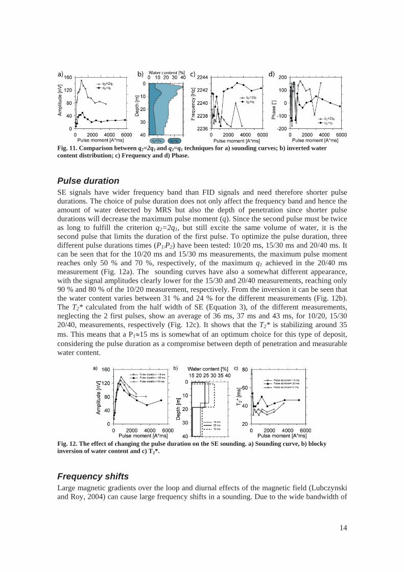
14
Fig. 11. Comparison between q2=2q1 and q2=q1 techniques for a) sounding curves; b) inverted water content distribution; c) Frequency and d) Phase.
Pulse duration SE signals have wider frequency band than FID signals and need therefore shorter pulse durations. The choice of pulse duration does not only affect the frequency band and hence the amount of water detected by MRS but also the depth of penetration since shorter pulse durations will decrease the maximum pulse moment (q). Since the second pulse must be twice as long to fulfill the criterion q2=2q1, but still excite the same volume of water, it is the second pulse that limits the duration of the first pulse. To optimize the pulse duration, three different pulse durations times (P1/P2) have been tested: 10/20 ms, 15/30 ms and 20/40 ms. It can be seen that for the 10/20 ms and 15/30 ms measurements, the maximum pulse moment reaches only 50 % and 70 %, respectively, of the maximum q1 achieved in the 20/40 ms measurement (Fig. 12a). The sounding curves have also a somewhat different appearance, with the signal amplitudes clearly lower for the 15/30 and 20/40 measurements, reaching only 90 % and 80 % of the 10/20 measurement, respectively. From the inversion it can be seen that the water content varies between 31 % and 24 % for the different measurements (Fig. 12b). The T2* calculated from the half width of SE (Equation 3), of the different measurements, neglecting the 2 first pulses, show an average of 36 ms, 37 ms and 43 ms, for 10/20, 15/30 20/40, measurements, respectively (Fig. 12c). It shows that the T2* is stabilizing around 35 ms. This means that a P1 15 ms is somewhat of an optimum choice for this type of deposit, considering the pulse duration as a compromise between depth of penetration and measurable water content.
Fig. 12. The effect of changing the pulse duration on the SE sounding. a) Sounding curve, b) blocky inversion of water content and c) T2*.
Frequency shifts Large magnetic gradients over the loop and diurnal effects of the magnetic field (Lubczynski and Roy, 2004) can cause large frequency shifts in a sounding. Due to the wide bandwidth of
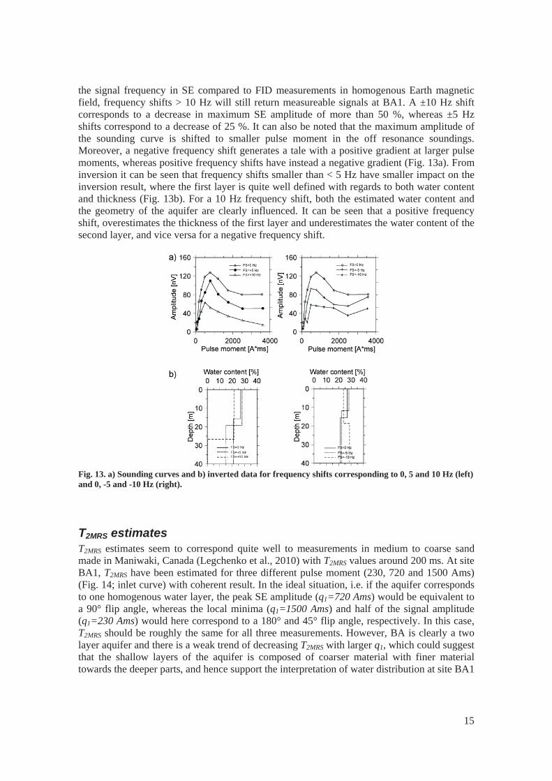
15
the signal frequency in SE compared to FID measurements in homogenous Earth magnetic field, frequency shifts > 10 Hz will still return measureable signals at BA1. A ±10 Hz shift corresponds to a decrease in maximum SE amplitude of more than 50 %, whereas ±5 Hz shifts correspond to a decrease of 25 %. It can also be noted that the maximum amplitude of the sounding curve is shifted to smaller pulse moment in the off resonance soundings. Moreover, a negative frequency shift generates a tale with a positive gradient at larger pulse moments, whereas positive frequency shifts have instead a negative gradient (Fig. 13a). From inversion it can be seen that frequency shifts smaller than < 5 Hz have smaller impact on the inversion result, where the first layer is quite well defined with regards to both water content and thickness (Fig. 13b). For a 10 Hz frequency shift, both the estimated water content and the geometry of the aquifer are clearly influenced. It can be seen that a positive frequency shift, overestimates the thickness of the first layer and underestimates the water content of the second layer, and vice versa for a negative frequency shift.
Fig. 13. a) Sounding curves and b) inverted data for frequency shifts corresponding to 0, 5 and 10 Hz (left) and 0, -5 and -10 Hz (right).
T2MRS estimates T2MRS estimates seem to correspond quite well to measurements in medium to coarse sand made in Maniwaki, Canada (Legchenko et al., 2010) with T2MRS values around 200 ms. At site BA1, T2MRS have been estimated for three different pulse moment (230, 720 and 1500 Ams) (Fig. 14; inlet curve) with coherent result. In the ideal situation, i.e. if the aquifer corresponds to one homogenous water layer, the peak SE amplitude (q1=720 Ams) would be equivalent to a 90° flip angle, whereas the local minima (q1=1500 Ams) and half of the signal amplitude (q1=230 Ams) would here correspond to a 180° and 45° flip angle, respectively. In this case, T2MRS should be roughly the same for all three measurements. However, BA is clearly a two layer aquifer and there is a weak trend of decreasing T2MRS with larger q1, which could suggest that the shallow layers of the aquifer is composed of coarser material with finer material towards the deeper parts, and hence support the interpretation of water distribution at site BA1
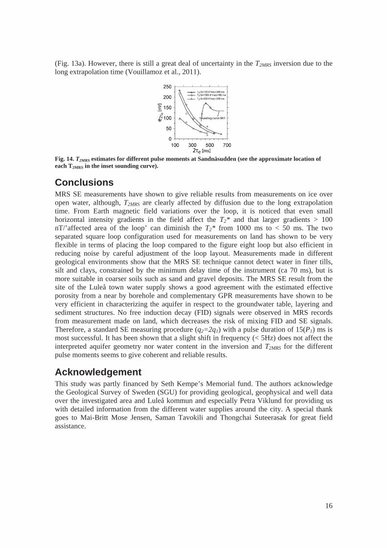
16
(Fig. 13a). However, there is still a great deal of uncertainty in the T2MRS inversion due to the long extrapolation time (Vouillamoz et al., 2011).
Fig. 14. T2MRS estimates for different pulse moments at Sandnäsudden (see the approximate location of each T2MRS in the inset sounding curve).
Conclusions MRS SE measurements have shown to give reliable results from measurements on ice over open water, although, T2MRS are clearly affected by diffusion due to the long extrapolation time. From Earth magnetic field variations over the loop, it is noticed that even small horizontal intensity gradients in the field affect the T2* and that larger gradients > 100 nT/’affected area of the loop’ can diminish the T2* from 1000 ms to < 50 ms. The two separated square loop configuration used for measurements on land has shown to be very flexible in terms of placing the loop compared to the figure eight loop but also efficient in reducing noise by careful adjustment of the loop layout. Measurements made in different geological environments show that the MRS SE technique cannot detect water in finer tills, silt and clays, constrained by the minimum delay time of the instrument (ca 70 ms), but is more suitable in coarser soils such as sand and gravel deposits. The MRS SE result from the site of the Luleå town water supply shows a good agreement with the estimated effective porosity from a near by borehole and complementary GPR measurements have shown to be very efficient in characterizing the aquifer in respect to the groundwater table, layering and sediment structures. No free induction decay (FID) signals were observed in MRS records from measurement made on land, which decreases the risk of mixing FID and SE signals. Therefore, a standard SE measuring procedure (q2=2q1) with a pulse duration of 15(P1) ms is most successful. It has been shown that a slight shift in frequency (< 5Hz) does not affect the interpreted aquifer geometry nor water content in the inversion and T2MRS for the different pulse moments seems to give coherent and reliable results.
Acknowledgement This study was partly financed by Seth Kempe’s Memorial fund. The authors acknowledge the Geological Survey of Sweden (SGU) for providing geological, geophysical and well data over the investigated area and Luleå kommun and especially Petra Viklund for providing us with detailed information from the different water supplies around the city. A special thank goes to Mai-Britt Mose Jensen, Saman Tavokili and Thongchai Suteerasak for great field assistance.
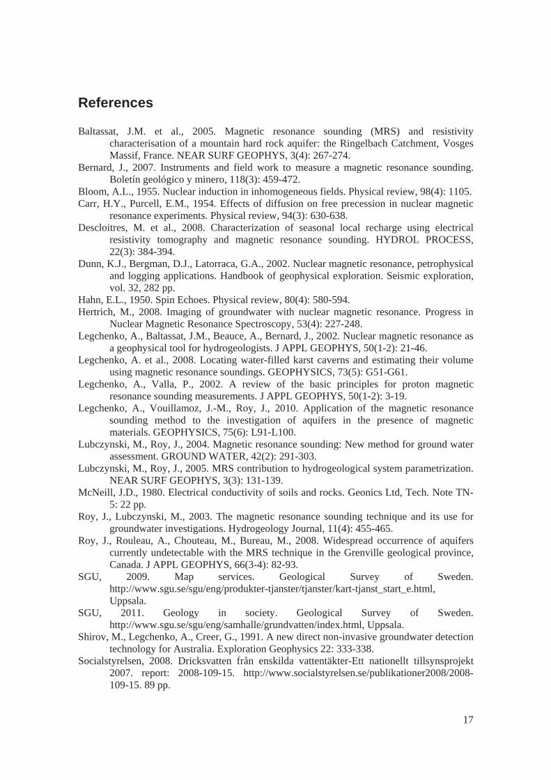
17
References Baltassat, J.M. et al., 2005. Magnetic resonance sounding (MRS) and resistivity
characterisation of a mountain hard rock aquifer: the Ringelbach Catchment, Vosges Massif, France. NEAR SURF GEOPHYS, 3(4): 267-274.
Bernard, J., 2007. Instruments and field work to measure a magnetic resonance sounding. Boletín geológico y minero, 118(3): 459-472.
Bloom, A.L., 1955. Nuclear induction in inhomogeneous fields. Physical review, 98(4): 1105. Carr, H.Y., Purcell, E.M., 1954. Effects of diffusion on free precession in nuclear magnetic
resonance experiments. Physical review, 94(3): 630-638. Descloitres, M. et al., 2008. Characterization of seasonal local recharge using electrical
resistivity tomography and magnetic resonance sounding. HYDROL PROCESS, 22(3): 384-394.
Dunn, K.J., Bergman, D.J., Latorraca, G.A., 2002. Nuclear magnetic resonance, petrophysical and logging applications. Handbook of geophysical exploration. Seismic exploration, vol. 32, 282 pp.
Hahn, E.L., 1950. Spin Echoes. Physical review, 80(4): 580-594. Hertrich, M., 2008. Imaging of groundwater with nuclear magnetic resonance. Progress in
Nuclear Magnetic Resonance Spectroscopy, 53(4): 227-248. Legchenko, A., Baltassat, J.M., Beauce, A., Bernard, J., 2002. Nuclear magnetic resonance as
a geophysical tool for hydrogeologists. J APPL GEOPHYS, 50(1-2): 21-46. Legchenko, A. et al., 2008. Locating water-filled karst caverns and estimating their volume
using magnetic resonance soundings. GEOPHYSICS, 73(5): G51-G61. Legchenko, A., Valla, P., 2002. A review of the basic principles for proton magnetic
resonance sounding measurements. J APPL GEOPHYS, 50(1-2): 3-19. Legchenko, A., Vouillamoz, J.-M., Roy, J., 2010. Application of the magnetic resonance
sounding method to the investigation of aquifers in the presence of magnetic materials. GEOPHYSICS, 75(6): L91-L100.
Lubczynski, M., Roy, J., 2004. Magnetic resonance sounding: New method for ground water assessment. GROUND WATER, 42(2): 291-303.
Lubczynski, M., Roy, J., 2005. MRS contribution to hydrogeological system parametrization. NEAR SURF GEOPHYS, 3(3): 131-139.
McNeill, J.D., 1980. Electrical conductivity of soils and rocks. Geonics Ltd, Tech. Note TN-5: 22 pp.
Roy, J., Lubczynski, M., 2003. The magnetic resonance sounding technique and its use for groundwater investigations. Hydrogeology Journal, 11(4): 455-465.
Roy, J., Rouleau, A., Chouteau, M., Bureau, M., 2008. Widespread occurrence of aquifers currently undetectable with the MRS technique in the Grenville geological province, Canada. J APPL GEOPHYS, 66(3-4): 82-93.
SGU, 2009. Map services. Geological Survey of Sweden. http://www.sgu.se/sgu/eng/produkter-tjanster/tjanster/kart-tjanst_start_e.html, Uppsala.
SGU, 2011. Geology in society. Geological Survey of Sweden. http://www.sgu.se/sgu/eng/samhalle/grundvatten/index.html, Uppsala.
Shirov, M., Legchenko, A., Creer, G., 1991. A new direct non-invasive groundwater detection technology for Australia. Exploration Geophysics 22: 333-338.
Socialstyrelsen, 2008. Dricksvatten från enskilda vattentäkter-Ett nationellt tillsynsprojekt 2007. report: 2008-109-15. http://www.socialstyrelsen.se/publikationer2008/2008-109-15. 89 pp.
18
SWECO, 2007. GÄDDVIKS VATTENTÄKT, Beskrivning, översiktliga optimeringsanvisningar och driftplan, Göteborg, 356 pp.
Tikhonov, A., Arsenin, V., 1977. Solutions of ill-posed problems. John Wiley & Sons, Washington DC, 258 pp.
Trushkin, D.V., Shushakov, O.A., Legchenko, A.V., 1994. The Potential of a Noise-Reducing Antenna for Surface NMR Groundwater Surveys in the Earths Magnetic-Field. Geophysical Prospecting, 42(8): 855-862.
Wattanasen, K., Elming, S.A., 2008. Direct and indirect methods for groundwater investigations: A case-study of MRS and VES in the southern part of Sweden. J APPL GEOPHYS, 66(3-4): 104-117.
Vouillamoz, J.M., Legchenko, A., Nandagiri, L., 2011. Characterizing aquifers when using magnetic resonance sounding in a heterogeneous geomagnetic field. NEAR SURF GEOPHYS, 9: 135-144.


