Radio sounding in space: magnetosphere and topside ionosphere

Journal of Atmospheric and Solar-Terrestrial Physics 63 (2001) 87–98www.elsevier.nl/locate/jastp

Radio sounding in space: magnetosphere and topsideionosphere

B.W. Reinischa ; ∗, D.M. Hainesa, R.F. Bensonb, J.L. Greenb,G.S. Salesa,W.W.L. TaylorcaCenter for Atmospheric Research, University of Massachusetts Lowell, 600 Su�olk Street, Lowell, MA 01854, USA

bNASA Goddard Space Flight Center, Code 630, Greenbelt, MD 20771, USAcRaytheon ITTS=GSFC, Code 630, Greenbelt, MD 20771, USA

Received 12 November 1999; accepted 21 January 2000

Abstract

Modern sounding techniques have been developed for the space-borne exploration of Earth’s magnetosphere and topsideionosphere. Two new satellite instruments will use the advanced techniques of the ground-based Digisondes. The RadioPlasma Imager (RPI), a low-frequency sounder with 500-m dipole antennas designed to sweep from 3 kHz to 3 MHz, will bepart of NASA’s IMAGE mission to be launched in February 2000 into an elliptical orbit with an altitude at apogee of 7Re.While in the magnetospheric cavity, RPI will receive echoes from the magnetopause and the plasmasphere and will measurethe direct response of the magnetosphere’s con�guration to changes in the solar wind. With three orthogonal dipole antennas(two 500-m tip-to-tip antennas in the spin plane used for transmission and reception, one 20-m antenna along the spin axisfor reception only) the arrival angle of returning echoes can be determined with high accuracy. The other instrument is theTOPside Automated Sounder (TOPAS), which was originally conceived for the Ukrainian WARNING mission with a launchdate in 2001. Using one antenna for transmission and three orthogonal 10-m antennas for reception, TOPAS will be able todetermine the arrival angle of ionospheric echoes and their wave polarization. It will then be possible to automatically scalethe topside ionograms and calculate the electron density pro�les in real time. Operating as a high-frequency radar, TOPASwill for the �rst time measure topside plasma velocities by tracking the motions of plasma irregularities. c© 2001 ElsevierScience Ltd. All rights reserved.

Keywords: Radio sounding; Magnetosphere; Topside ionosphere

1. Introduction

Radio sounding is a well-established technique that was�rst deployed in the 1920s for ionospheric sounding fromthe ground (Breit and Tuve, 1926). In recent years, advanceddigital sounders have been developed for ground-based ob-servations that provide detailed information about the struc-ture and dynamics of the bottomside ionosphere (Reinisch,1996). These modern sounders measure more than justthe time of ight and amplitude of the echoes, they also

∗ Corresponding author. Tel.: +1-978-934-4903; fax: +1-978-459-7915.E-mail address: bodo [email protected] (B.W. Reinisch).

determine the arrival angle, wave polarization and Dopplerfrequency. Radio sounding relies on total re ection of radiowaves from plasma structures that have a plasma frequencyfN equal to the radio frequency f. It is, therefore, not possi-ble to receive echoes re ected from the topside ionosphereor the magnetosphere on the ground since the F2 layerprevents all transmitted waves with frequencies f¡fo F2from propagating beyond the height of the F2 layer peak.Topside ionospheric sounders, �rst described by Franklinand Maclean (1969), recorded the amplitudes and echo de-lay times of ionospheric echoes as a function of frequency inthe same way as it was done by the ground-based soundersof the time. Data from the highly successful Alouette=ISIStopside sounders (Jackson et al., 1980; Jackson, 1986) were

1364-6826/01/$ - see front matter c© 2001 Elsevier Science Ltd. All rights reserved.PII: S1364 -6826(00)00133 -4

88 B.W. Reinisch et al. / Journal of Atmospheric and Solar-Terrestrial Physics 63 (2001) 87–98

Fig. 1. (a) RPI transmits omidirectionally and can receive echoesfrom the magnetopause, plasmapause and the cusp. Two orthogonal500-m dipoles are used for transmission. (b) Vertical and obliqueechoes received by a topside sounder. The Doppler shifts of theecho signals are proportional to the di�erence between the satellitevelocity vs and the velocity vl of the irregularities.

the basis for nearly 1000 scienti�c publications (Bensonet al., 1998). The typical frequency range of the analogsounders was 0.1–20 MHz (Pulinets, 1989) correspondingto the plasma frequencies in the ionosphere. For magne-tospheric sounding, the required frequency range is 3 kHzto 3 MHz, corresponding to electron densities Ne≈ 105–1011 m−3, since fN=Hz≈ 9

√Ne=m−3. The cartoons in

Fig. 1 illustrate the geometries for magnetosphericand topside sounding. As discussed below, transmis-sion will be nearly omnidirectional and echoes canbe returned from many directions. In the magneto-spheric case, the possible arrival angles cover thefull sphere, and for topside sounding the lower half-sphere.

To correctly interpret the echoes in terms of plasma den-sity and echo location it is, therefore, necessary to determinethe arrival angles of the echoes together with the distanceto the re ection point and the wave polarization. Section 4describes how the polarization ellipse and the angle ofarrival are determined from in-phase and quadratureSAMPLES of the signals from three orthogonal antennas.Ionospheric sounders on the ground usually use interfero-metric techniques with three or more spaced antennas todetermine the arrival angle, and crossed dipoles to �nd thepolarization (Reinisch, 1996). A single-point measurementof these quantities with three orthogonal antennas on theground is di�cult to carry out because of the ground ef-fects, but it can in principle be done (Afraimowich et al.,1999; Marie et al., 1999). Both the interferometric andthe single point technique assume that only one signal offrequency f arrives at a given time at the receive antennas.This condition is normally not satis�ed since echoes fromdi�erent directions will superimpose. For pulsed signals,only echoes from targets with a virtual distance betweenR′ and R′ + c PW=2 will superimpose where c is thefree-space speed of light and PW the pulse width. The vir-tual distance, or range, is de�ned as R′ =0:5c te where te isthe measured echo travel time. Pulsing the transmit signalreduces the number of time-coincident echoes, but therecan still be many echoes dependent on the structure of theplasma which would void the direction �nding techniquesreferenced above. Bibl and Reinisch (1978) overcame thisdi�culty by �rst Fourier analyzing the echo signals, thusseparating any time-coincident echoes by making use of thedirection-dependent Doppler shifts. It is very unlikely thatechoes from di�erent directions have the same propagationdelay between te and te + PW=2 and the same Doppler shiftd= K · (v − vS)=�, where K = (2�=�)n is the wave vector,v is the target velocity, vS is the spacecraft velocity, � isthe free-space wavelength, and n is the wave normal. Thisecho source identi�cation technique, using interferometricDoppler imaging (IDI), had been pioneered for ionosphericradio sounding from the ground (where vS = 0) by Bibl andReinisch (1978), but is equally applicable in space wherethe single-point direction �nding technique replaces theinterferometry.Modern sounding techniques will now be applied to the

remote sensing of plasma structures above the peak of theF2 layer. The radio plasma imager (RPI) will be ying onNASA’s magnetospheric IMAGER satellite to be launchedin February 2000, and the TOPAS is being developed fora satellite orbiting at ∼ 1000 km altitude. Both instrumentsuse in-phase and quadrature sampling of signals received onthree orthogonal antennas and advanced signal processingtechniques including pulse compression and Fourier integra-tion. The instruments and the di�erent waveforms used arebrie y described in Sections 2 and 3. The calculations ofthe polarization ellipse, the wave mode, and the arrival an-gle, which are the same for both instruments, are discussedin Section 4.

B.W. Reinisch et al. / Journal of Atmospheric and Solar-Terrestrial Physics 63 (2001) 87–98 89

2. The radio plasma imager on the IMAGE mission

NASA’s IMAGE mission is scheduled for launch fromVandenberg AFB, CA, in March 2000. The 14.5-h orbit willbe highly elliptical with 7Re altitude at apogee and 1000km at perigee. The mission’s scienti�c objective is to deter-mine the dynamic characteristics of the magnetosphere inresponse to changes in the solar wind. The changing charac-teristics of the magnetospheric plasma structures, from themagnetopause to the auroral ionosphere, can be captured byremote sensing from a single satellite using imaging tech-niques. IMAGE, which will be NASA’s �rst Medium-classExplorer (MIDEX) mission, will carry three di�erent typesof sensors: neutral atom, UV and the radio plasma imagers.Burch of Southwest Research Institute in San Antonio, TX,is the principal investigator of the IMAGE mission (Burch,2000).

2.1. The RPI instrument

The RPI functions as a radar, transmitting radio wavessimultaneously into all directions and measuring the arrivalangle and delay time of all echoes (Reinisch et al., 2000;Green et al., 1998). It will use three orthogonal thin-wiredipole antennas for reception, two of which are 500-mtip-to-tip dipole antennas in the spin plane; these two dipolesare also used for transmission. The third antenna, along thespin axis, is 20m long and is used for reception only. Thethree thin-wire dipole antennas and their deployers havebeen designed and built by Able Engineering Company(AEC). The antenna material is 7-strand BeCu wire witha diameter of 0.4 mm. The IMAGE spacecraft will have aspin rate of 0.5 rotations per minute, su�cient to keep thetwo 500-m dipoles with their tip masses of 50 g in stablepositions. A thin-wire antenna is also required for the dipolealong the spin axis in order to minimize the photoelectricnoise that can a�ect the quasi-thermal noise spectroscopymeasurements (Meyer-Vernet et al., 1998) RPI plans tocarry out. Two self-erecting �berglass lattice booms extendthe two 10-m wires to their measurement positions.Right- and left-hand polarized signals will be transmitted

by feeding the currents into the long-wire antennas 90◦ outof phase as discussed by Reinisch et al. (2000) in an RPIinstrument paper. This produces a nearly isotropic radiationpattern with maxima in the direction of the spin axis anda 3 dB minimum in the spin plane (Reinisch et al., 1999).In a feasibility paper (Calvert et al., 1995), we have shownthat a 10 W transmitter together with low-noise receiversprovide adequate signal-to-noise ratios to determine rangeand direction of echo signals up to a distance of at least5Re. Unlike radio sounding on the ground, magnetosphericsounding is not limited by the interference from man-madesources, but by natural external noise. Moderately intenseto intense natural noises, in RPI’s frequency range, consistof Type III solar-noise bursts and storms, auroral kilometricradiation (AKR), and the non-thermal continuum (escaping

and trapped). These natural noises have the potential to a�ectRPI’s ability to clearly distinguish the echoes that will begenerated. However, due to several mitigation strategies anda favorable orbit, RPI should be able to operate withoutsigni�cant impact from these natural noises.Natural noise takes several forms. Type III solar

storms consist of thousands of Type III bursts producedquasi-continuously, resulting in broadband emissions. Thefrequency range for Type III emissions extends from abovethe RPI maximum frequency of 3 MHz to the lowestfrequencies that can propagate through the earth’s magne-tosheath, typically 30 to 100 kHz. Type III bursts are nearlyas intense as the most intense AKR, whereas Type III solarstorms have typical power uxes only about an order ofmagnitude above the cosmic noise background (Benson andFainberg, 1991; Bougeret et al., 1984). Type III bursts willbe observed by RPI in any location in its orbit making echodetection extremely di�cult while they last; however, theyare relatively rare and will not a�ect detection of echoes atlower frequencies. AKR is associated with auroral arcs andoriginates above auroral regions at about one half to a fewRe altitude. The frequency of the emission is from about 30to about 700 kHz with peak emission between 100 and 400kHz, depending on local time and magnetic activity. Themaximum power for AKR is many orders of magnitudeabove the cosmic and receiver noise. Propagation e�ects(see Green et al., 1977) restrict AKR to higher magneticlatitudes over certain local times. Fortunately, both O andX mode AKR are very narrowband, in the order of 1 kHzor less (Gurnett and Anderson, 1981; Benson et al., 1988).In this case, RPI’s frequency agility capability will be im-portant and it is expected that AKR will not pose a majorproblem in RPI’s ability to generate and detect echoes be-tween AKR narrowbanded emissions. Continuum radiationhas two components, trapped and escaping (Gurnett, 1975).The trapped component ranges in frequency from about 30kHz to the magnetosheath fp, which is between 30 and 100kHz. The frequency range of the escaping component variesfrom the magnetosheath fp (∼ 30 kHz) to a few hundredkHz. Continuum radiation is believed to be generated pri-marily in the O mode. The source region appears to benear the low-latitude plasmapause, primarily on the dawnsector. In a recent study by Green and Boardsen (1999),the angular distribution of the non-thermal continuum ra-diation was studied with observations from the Hawkeyespacecraft and modeled with ray tracing calculations. Fromthese results it is clear that the trapped continuum radiationdoes not uniformly illuminate the magnetospheric cavitybut is mainly con�ned to low latitudes. Thus, RPI shouldrarely encounter continuum radiation since IMAGE will bein a high-inclination orbit. In comparison to these naturalnoises, the receiver and cosmic noise are of less importance.Fig. 2 shows the system con�guration for RPI. The elec-

tronics, including two transmitter exciters, three receivers,and digital control and power circuits, are contained on sixprinted circuit boards mounted inside the main chassis. The


Fig. 2. RPI instrument con�guration.

Fig. 3. RPI transmitter and antenna coupler for one antenna element.

two exciters drive four RF ampli�ers, each feeding the RFcurrent through a tuning coupler to a 250-m antenna. InFig. 3, the RF ampli�er is identi�ed as a transmitter consist-ing of a variable 6 to 24 V power supply and two FET am-

pli�ers driving a step-up transformer. The variable supplyvoltage is controlled to limit the voltage at the antenna feedpoint to 1:5 kVrms, i.e., 3 kVrms between antenna terminals,reducing the risk of arcing. For f¡ 300 kHz, the antennaimpedance is capacitive with a reactance of Xa=1=!C wherethe capacitance of the 500-m dipole is C = 533 pF. The ra-diated power is Pr = I 2a Rr where Ia is the antenna current andRr the radiation resistance. For a short thin-wire dipole theradiation resistance is Rr =20�2 (L=�)2 (Kraus, 1988 Chap-ter 5), where L = 500 m for RPI, and � is the wavelength.By measuring the antenna current we were able to deter-mine the radiated power as function of frequency. Fig. 4shows the power radiated by each 250-m antenna element. A10 W power maximum is imposed by spacecraft powerlimitations.


Fig. 4. Variation with frequency of the RF power radiated by oneantenna element. Below ∼ 280 kHz, the power is limited by theimposed voltage maximum of 1:5 kVrms. At the higher frequencies,the power supply voltage is reduced to limit the radiated power to∼ 10W.

The entire RPI operation is controlled by the SC7 centralprocessing unit (CPU) in the main chassis. The space qual-i�ed SC7, built by Southwest Research Institute, is basedon a Texas Instruments TMS320C30 digital signal proces-sor. The CPU controls all analog and digital operationsincluding frequency synthesis, receiver gain selection, wave-form shaping and timing, signal processing, and measure-ment programming. Each of the six antenna elements drivesa high-impedance, low-noise preampli�er mounted at theantenna feed point (Fig. 2). The preampli�ers have been de-signed to recover rapidly from the high voltage generatedduring the transmitter pulses. The 300-Hz receiver band-width, matched to the bandwidth of the transmitted wave-form (Table 1), provides a range resolution of 480 km. The�nal intermediate frequency signal at the receiver output,IF = 45 kHz, is digitized, and digital-signal processing isapplied depending on the selected operational waveforms.The overall system sensitivity limit is about 8 nV=

√Hz for

the Z receiver connected to the short antenna along the spinaxis, and 25 nV=

√Hz for the X and Y receivers connected

to the long antennas in the spin plane. The corresponding�eld strength sensitivities are therefore ∼ 800 pV=m for thez component and ∼ 100 pV=m for the x and y components.Internal calibration signals are fed to the receiver inputs be-fore the transmission for each selected frequency to calibratethe receiver gains.The RPI receivers are specially designed for tolerance to

the high-level transmitter pulse and recovery to full sensi-tivity within less than 7 ms. This fast recovery time of lessthan two reciprocal bandwidths is made possible by twospecial design features. Firstly, the 300-Hz receiver band-width is the result of seven tuned stages of receiver IF, eachwith a bandwidth of 1 kHz. The tuning is performed withferrite-loaded transformers and inductors, which are criti-cally tuned based on the magnetic permeability of the ferritecore material. When a stage of the receiver is saturated, the

currents are su�cient to depress the e�ective permeabilityof the tuned circuit in that stage. This core saturation de-tunes the stage thereby reducing the amplitude of the signalpassed on to the next stage. During the transmitter pulse,all stages are bordering on saturation and it is important todischarge the tuned circuits as quickly as possible after thetransmit pulse in order to be ready for echo signal recep-tion. Secondly, a �xed receiver gain is set before any pulsesare transmitted, eliminating any consideration of an auto-matic gain control (AGC) response time. The receivers havean instantaneous dynamic range of 60 dB. In addition, thecomputer controlled AGC can vary the receiver gain by 66dB, resulting in an overall signal operating range of 126 dB,from 0 to −126 dB m. The sensitivity is increased furtherby the pulse compression and signal integration with a typi-cal signal processing gain of ∼ 20 dB, resulting in a systemsensitivity of −146 dB m or about 12 nVrms. This sensitiv-ity will enable RPI to detect pulse echoes from ranges inexcess of 5Re. The output of the X, Y and Z receivers is a 45kHz intermediate frequency (IF) signal, which is digitizedtaking in-phase and quadrature samples every 1.6 s. Table 1summarizes the speci�cations for the RPI instrument.

2.2. Waveforms and signal processing

Because of the largely unknown magnitude of transportvelocities of plasma structures or wave velocities in the mag-netopause, the coherence and the Doppler characteristics ofthe expected RPI echoes can only be estimated. Therefore,RPI was designed with several waveforms of widely vary-ing characteristics. The capability of the various waveformsis intimately related to the algorithms used to process theecho returns.

2.2.1. Coherent integrationThe critical issue in selection of a waveform is the coher-

ence time of the medium (Fung et al., 2000). The coherencetime is the interval during which the phase of each of the si-nusoidal components in an echo signal does not signi�cantlychange, that is, the complex amplitudes of successive sam-ples of the same echo will sum in phase when accumulatedover the integration period. If the signal samples are not co-herent then the mean amplitude of the accumulated sum ofN samples will be larger than a single sample by the squareroot of N , which is the same increase that is achieved whenintegrating random noise. However, if the multiple samplesare coherent, the amplitude of the accumulated sum is Ntimes a single sample, which is root N larger than the ac-cumulated noise component of the signal, and therefore in-creases detectability, even for signals which are weaker thanthe received noise. It would appear then that any Dopplershift large enough to change the phase of a signal by morethan 90◦ during the integration would ruin the coherence.Spectral integration, however, corrects this phase shift foreach resolvable Doppler frequency, thereby allowing coher-ent integration for any signal that has a constant Doppler


Table 1RPI speci�cations

System parameter Nominal Limits Rationale

Radiated power 10 W at 5 to 10 W per antenna Required for adequate SNR20% duty cycle element

Frequency range 3 kHz–3 MHz Covers expected range of plasmadensities.

Freq. accuracy 1× 10−5 Accurately measures observed plasmadensities.

Freq. steps 5% steps ¿ 100 Hz 5% in frequency gives 10% in plasmadensity resolution.

Measurement duration 1 s to ∼ minutes 50 ms Di�erent spatial and temporalrequirements along orbit

Maximum virtual 120,000 km 300,000 km Extent of expected magnetosphericrange echo rangesMinimum virtual 980 km with 3.2 ms 0 km for passive Pulse width + receiver recovery time is 7 msrange short pulses modesRange increments 240 km 240 or 480 km Required sampling resolutionPulse rep rate 1 s−1 0.5–20 s−1 Sets unambiguous rangePulse width 3.2 ms 3.2 ms–1.9 s Provide 480 km range resolutionReceiver bandwidth 312 Hz Consistent with 3.2 ms pulse widthReceiver sensitivity 25 nV=

√Hz (X & Y); Keeps receiver noise below cosmic

8 nV=√Hz (Z) noise

Coherent integration 8 s 125 ms–64 s Provides both processing gain &time Doppler resolutionDoppler resolution 125 mHz Determined by coherent integration

timeReceiver saturation 6 ms Specially designed monostatic radarrecovery receiverDoppler range ±2 Hz ±150 Hz To measure expected plasma velocitiesAmplitude resolution 3 dB 3=8 dB Data format allows 3=8 dB, but typical

display is 3 dBAngle-of-arrival 2◦ 1◦ when SNR is Identify echo direction with requiredresolution 40 dB or better accuracyAntenna length 10 and 250 m SNR requiredProcessing gain 21 dB 0–33 dB To enhance weak echoesMass incl. antennas 56 kgAverage power 32 W

over the integration period. The characteristics that limit co-herent integration time have to do with the extent to whichthe observed object is accelerating, since such accelerationleads to glinting, blinking or twinkling. The RPI instrumentuses a variety of waveforms to ensure target detection inthe presence of high Doppler shifts, acceleration or rapidlychanging objects.

2.2.2. Natural noise mitigationNatural noise, including auroral kilometric radiation

(AKR) will interfere with the reception of weak echoes.Since the frequency spectrum of AKR noise is highly vari-able it will generally be possible to �nd quiet frequencieswith low noise. A “frequency search” technique is there-fore used at each nominal sounding frequency just priorto the transmission of the pulse or the sequence of pulses.Five frequencies spaced by 300 Hz are tested around the

nominal frequency, and the one with the lowest noise levelis selected for sounding.

2.2.3. Evenly spaced pulse sequences and their limitationsTo provide a detection range of 60,000 or 120,000 km

requires a pulse repetition rate of 2 or 1Hz, respectively, inorder to avoid range aliasing. With such a slow repetitionrate, several seconds are required to integrate repeated pulsetransmissions. For instance, the integration of 16 pulsesspaced by 0.5 s, requiring 8 s of integration time, providesa 12 dB signal-to-noise enhancement if the signal remainscoherent for this time. Since this is not assured we haveprovided the 16-chip complimentary phase code and theFM chirp waveforms that provide 12 and 18 dB of signalenhancement, respectively, within one second (see below).A serious disadvantage of evenly spaced pulses is themaximum Doppler frequency that can be unambiguously


sampled, which is half the repetition rate. Very fast mov-ing structures, such as plasmoids and waves in the mag-netopause, are estimated to produce tens of Hz Dopplershifts leading to aliasing, i.e., fold-over in the computedDoppler spectrum. The pulse repetition rate is equal to thedata-sampling rate, since for each range one data sampleis obtained after each transmitted 3.2 ms pulse. If the echofrequency is shifted by tens of Hz, it becomes quite mean-ingless to produce a Doppler spectrum from the repeatedpulse echoes. For such high Doppler conditions, the FMchirp pulse can be used to achieve a similar processing gainusing only a single pulse. This single-pulse technique doesnot, however, provide a Doppler spectrum. On the otherhand, Doppler processing is desired to determine the radialvelocity of the observed structures; also, as discussedearlier, Doppler separation is a prerequisite for arrival anglemeasurements.

2.2.4. Long pulseTo measure the true radial velocity of very fast moving

plasma irregularities, RPI can use the long-pulse waveform.The long pulse of either 125 or 500 ms duration is longenough to provide a Doppler spectrum with a resolutionsomewhere between 2 and 8 Hz, and a Doppler range of±150 Hz, limited only by the 300 Hz analog bandwidth ofthe receiver. Of course, these long pulses provide no usefulrange resolution.

2.2.5. Staggered pulse sequenceThe staggered pulse sequence (SPS) provides the same

Doppler range, but also provides range information with480-km resolution. It consists of 212 pseudo-randomlyspaced 3.2-ms pulses transmitted in about 2.5 s (Reinischet al., 2000). Echoes from previously transmitted pulses arereceived in the listening time between transmissions. Anecho received during a given listening time may have comefrom any of the preceding transmitted pulses, therefore theprocessing algorithm provides discrimination of one rangeversus another, but there is some inevitable leakage of en-ergy from one range to the others. A random phase shiftis applied to the transmitted signals and is removed uponreception, so successive echoes will coherently integrateonly for those echoes that result from the correct transmit-ted pulse, that is, those that experienced the time delay thatcorresponds to the range currently being processed.

2.2.6. FM chirpFor the detection of high Doppler echoes, the FM chirp

waveform can be used. The chirp waveform has a RF car-rier that is linearly increasing in frequency (Barry, 1971)modulated by a rectangular pulse. The RPI chirp waveformhas a sweep rate of 244 Hz in 0.125 s. The received signalsare mixed with a local oscillator signal which sweeps at thesame rate used for the transmitted pulse, and the di�erencefrequency is therefore linearly proportional to the time delay

of the echo. A spectral analysis of the down-converted sig-nal produces a range pro�le of all echoes received (Poole,1985). Since the receiver is linear, overlapping receptionof multiple echoes from di�erent ranges are resolved sincethey produce di�erent Fourier components.

2.3. RPI data products

It is di�cult to present RPI’s multi-dimensional sound-ing data in one image since, for each sounding frequency,echoes can arrive from all directions with di�erent delays(ranges). The most direct display is the plasmagram, whichis similar to the ionogram for ionospheric sounding. Theplasmagram does not show, however, from what directionthe echoes are arriving, and a complementary display is re-quired, the echo-map, to assess the 3-D plasma distributionin the magnetosphere.

2.3.1. PlasmagramsLike the ionogram for ionospheric sounding, the plasma-

gram gives the most complete visualization of the receivedsignals for magnetospheric sounding. It presents all signalsreceived in a frequency-versus-range frame. Fig. 5 showsa simulated plasmagram with simulated noise. The echoranges were calculated using ray tracing through a plasmadensity model that includes an ionosphere, plasmasphere,polar cap, cusp, magnetosphere and magnetopause. Theecho amplitudes were derived from the radiated power (seeFig. 3) and a �eld strength inversely proportional to thedistance. The actual �eld strengths may di�er by ∼ ± 6 dBsince the virtual range is larger than the distance, and be-cause of focussing and defocussing (Calvert et al., 1995).The noise consists of the band near the electron plasmafrequency, denoted by Fpe on the frequency axis, and theinstrument noise that was measured as a function of fre-quency. The echoes at a range of about 3Re are from themagnetopause. The echoes which extend from about 3Reand 6 kHz to about 5:5Re and 80 kHz are from the cusp,and the remaining echoes are from the magnetosphere,plasmasphere and ionosphere below the spacecraft. Actualplasmagrams can be expected to be much more complicated,containing spread traces, echoes from plasma irregularities,and multi-hop echoes. From the variation of the virtualecho ranges R′(f) with frequency, one can calculate theactual (or “true”) ranges R(f) and the plasma concentra-tion pro�le using the techniques developed for ionosphericionograms (Jackson, 1969; Huang and Reinisch, 1982).

2.3.2. Echo-mapsThe arrival angle (see Section 4) and range of an echo at

frequency f determine the location and plasma frequencyof the re ection point. The echo-map is a 2-D cross-sectionof the 3-D space, with all echoes projected into the orbitalplane. The intersection of this plane with the magnetopauseand plasmapause (Fung and Green, 1996) is shown to aidthe interpretation of the echoes. (Fig. 6). The echo range is


Fig. 5. Simulated plasmagram showing the signal amplitudes as function of range and frequency. Signal and noise amplitudes use the colorcode shown on the right.

Fig. 6. Simulated echo-map. The echo locations are projected into the orbital plane conserving echo range and azimuth angle. The echocolors identify the sounding frequency.


conserved by projecting each echo along an arc with radiusR′ into the echo-map. Thus, the echo locations on the 2-Dplane present both azimuth and range information. The col-ors of the echoes represent the sounding frequency, i.e.,the plasma frequency of the re ecting structure. Inherentin the construction of the echo-maps is the 180◦ ambiguityof the echo location as discussed in Section 4. We there-fore show the echo together with a “ghost” echo assumed toarrive from the opposite hemisphere. The browse display as-sumes one answer, shown in color, and indicates the ghostlocation in gray. In most instances it will be possible toresolve the 180◦ ambiguity by inspecting the plasmagramtraces and comparing the deduced echo locations with pre-dictions based on magnetospheric Ne models.

3. Topside sounder

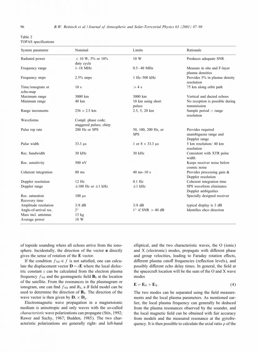
Originally planned for the Ukrainian satellite missionWARNING, the design of a topside automated sounder(TOPAS) followed the concepts developed for UML’ssuccessful ground-based ionosonde, the Digisonde PortableSounder (DPS) (Reinisch et al., 1997). The radio imagingtechnique uses the single point method described in Sec-tion 4. The instrument con�guration is very similar toRPI’s shown in Fig. 2. The instrument speci�cations,summarized in Table 2, di�er of course from RPI’s. Thefrequency range is from 0.5 to 30 MHz covering densi-ties from 109 to 1013 m−3. Three orthogonal 10-m an-tennas will be used for reception. To keep the total massdown, only one transmitter will be used to drive one ofthe antennas, which will be electronically tuned to op-timize the transmission e�ciency. Ten watts of radiatedpower will produce signal-to-noise ratios of 30 to 40dB, making use of the digital processing gain obtainedby applying the pulse compression and Fourier analysistechniques developed for the DPS. An additional wave-form, a staggered pulse sequence with 33.3 �s pulseswill expand the Doppler frequency range to ±1 kHz,large enough to avoid aliasing caused by the satellitemotion.By measuring the arrival angles and the Doppler shift of

the ionospheric echoes it will be possible to determine thevertical electron density pro�les in real time, and also tocalculate the velocity of ionospheric irregularities (Fig. 1b).After identifying and disregarding the o�-vertical echoes,the vertical echo traces can be automatically scaled and theNe pro�le calculated (Reinisch and Huang, 1982; Huang andReinisch, 1982). The availability of real time topside pro�leswill be a valuable input to space weather forecasting. Byanalyzing the Doppler frequencies for the di�erent echoesit will also be possible to determine the drift velocity of thetopside plasma irregularities similar to the Digisonde’s IDItechnique (Cannon et al., 1991; Scali et al., 1995; Smithet al., 1998).

4. Spaceborne radio imaging

Radio imaging from a single spacecraft can be done byusing three orthogonal receiver antennas. Since the trans-mission for low and high frequencies is nearly omnidirec-tional, the echo direction must be determined by measuringthe arrival angle of the received signals. Morgan and Evans(1951) had proposed the use of space-quadrature sinusoidalcomponents of the electric-�eld vector to determine thepolarization plane of an arriving plane wave for ground-based HF measurements. Afraimowich et al. (1999) ex-perimentally veri�ed this single-point technique using themethod of spectral decomposition of the received signalsintroduced by Bibl and Reinisch (1978). Shawhan (1970)proposed the use of orthogonal magnetic antennas for direc-tion �nding in space. Both sounders described in this paperuse electric antennas to measure the wave normal direction.Since for most echoes fNS.f with fNS being the plasmafrequency at the spacecraft location, the E �eld componentin the direction of the wave normal is negligible, and thenormal to the wave front is the wave direction.To �nd the polarization plane, the instruments determine

two vectors Ei and Eq (Fig. 7) from the quadrature samplesof the three antenna signals. We can write for the voltagesat the three receiver outputs:

Vx(t) = V̂xei(!t+�x);

Vy(t) = V̂yei(!t+�y);

Vz(t) = V̂zei(!t+�z): (1)

The peak voltages V̂m and the phases �m (m = x; y; z) aredetermined from the quadrature samples Im and Qm taken attimes !t = 0 and !t = �=2:

Im = V̂mei�m ; Qm = V̂me

i(�m+�=2): (2a)

V̂m =√I 2m + Q2m; �m = tan

−1QmIm: (2b)

The e�ective receiver gains need to be carefully adjustedso that the ratios Vm=Em = �m are the same for the threecomponents. The ratio �m can be expressed as the productof the e�ective antenna length L′ ≈ 0:5 La and the receivervoltage gain G, where La is the actual length of the an-tenna. For RPI, L′x = L

′; y ≈ 250 m; L′z ≈ 10 m; Gx = Gy,

and Gz = 25 Gx. For TOPAS, L′x = L′; y = L

′z ≈ 5 m, and

Gx =Gy; =Gz . Careful calibration is required to correct thedigital data for di�erences in �m for the three channels. Ifwe de�ne the quadrature vectors I = (Ix; Iy; Iz), and Q =(Qx;Qy;Qz) we can write for the wave normal

n =Ei × Eq|Ei × Eq| =

I ×Q|I ×Q| : (3)

This vector is parallel to the wave normal, but has a 180◦

ambiguity in its pointing direction that must be resolvedwith the help of the plasmagram and echo-map for the RPIobservations. This complication does not arise in the case


Table 2TOPAS speci�cations

System parameter Nominal Limits Rationale

Radiated power ¡ 10 W, 5% or 10% 10 W Produces adequate SNRduty cycle

Frequency range 1–18 MHz 0.5–40 MHz Measure in situ and F-layerplasma densities

Frequency steps 2.5% steps 1 Hz–500 kHz Provides 5% in plasma densityresolution

Time=ionogram or 10 s ¿ 4 s 75 km along orbit pathecho-mapMaximum range 3000 km 3000 km Vertical and ducted echoesMinimum range 40 km 10 km using short No reception is possible during

pulses transmissionRange increments 256× 2:5 km 2.5, 5, 20 km Sample period = range

resolutionWaveforms Compl. phase code;

staggered pulses; chirpPulse rep rate 200 Hz or SPS 50, 100, 200 Hz, or Provides required

SPS unambiguous range andDoppler range

Pulse width 33:3 �s 1 or 8× 33:3 �s 5 km resolution= 40 kmresolution

Rec. bandwidth 30 kHz 30 kHz Consistent with XTR pulsewidth

Rec. sensitivity 500 nV Keeps receiver noise belowcosmic noise

Coherent integration 80 ms 40 ms–10 s Provides processing gain &Doppler resolution

Doppler resolution 12 Hz 0.1 Hz Coherent integration timeDoppler range ±100 Hz or ±1 kHz ±1 kHz SPS waveform eliminates

Doppler ambiguitiesRec. saturation 100 �s Specially designed receiverRecovery timeAmplitude resolution 3=8 dB 3=8 dB typical display is 3 dBAngle-of-arrival res. 2◦ 1◦ if SNR ¿ 40 dB Identi�es ehco directionMass incl. antennas 13 kgAverage power 18 W

of topside sounding where all echoes arrive from the iono-sphere. Incidentally, the direction of the vector n directlygives the sense of rotation of the E vector.If the condition fNS.f is not satis�ed, one can calcu-

late the displacement vector D= �E where the local dielec-tric constant � can be calculated from the electron plasmafrequency fNS and the geomagnetic �eld BS at the locationof the satellite. From the resonances in the plasmagram orionogram, one can �nd fNS and BS, a B �eld model can beused to determine the direction of BS. The direction of thewave vector is then given by Di ×Dq.Electromagnetic wave propagation in a magnetoionic

medium is anisotropic and only waves with the so-calledcharacteristicwave polarizations can propagate (Stix, 1992;Rawer and Suchy, 1967; Budden, 1985). The two char-acteristic polarizations are generally right- and left-hand

elliptical, and the two characteristic waves, the O (ionic)and X (electronic) modes, propagate with di�erent phaseand group velocities, leading to Faraday rotation e�ects,di�erent plasma cuto� frequencies (re ection levels), andpossibly di�erent echo delay times. In general, the �eld atthe spacecraft location will be the sum of the O and X wavemodes

E = EO + EX : (4)

The two modes can be separated using the �eld measure-ments and the local plasma parameters. As mentioned ear-lier, the local plasma frequency can generally be deducedfrom the plasma resonances observed by the sounder, andthe local magnetic �eld can be obtained with fair accuracyfrom models and the measured resonance at the gyrofre-quency. It is then possible to calculate the axial ratio � of the


Fig. 7. The polarization ellipse with the semi-major axis, a and thesemi-minor axis b= �a. The vectors Ei and Eq are obtained fromthe quadrature samples at times !t = 0 and �=2.

characteristic polarization ellipses (Kelso, 1964). Reinischet al. (1999) expressed the �eld in the polarization planex′y′ in terms of the semi-major axes aO and aX of the po-larization ellipses of the O and X modes, and the phase dif-ference � between them. Equating the resulting expressionto the �eld measured on the x; y, and z antennas yields

E= [(aO + aX�ei�)x′ + (aO�− aXei�)y′]ei!t= [Exx + Eyy + Ezz]ei!t : (5)

Ex; Ey and Ez are the measured �eld components, and theparameters aO; aX, and �, characterizing the polarization el-lipses, can therefore be calculated from the three componentequations in (5).

5. Summary

Modern radio sounders in space open new possibilitiesfor the exploration of space plasmas. Alternate waveformsand advanced signal processing have reduced the powerand mass requirements previously associated with radiosounding. The use of three orthogonal receiver antennasand in-phase and quadrature sampling of the three antennasignals, combined with complex spectral analysis, make itpossible to determine the arrival angles of the echoes thus“imaging” the plasma boundaries and irregularities. TheDoppler measurements give information about the veloci-ties of the plasma structures. Both of the two instrumentsdescribed will provide new and much needed informa-tion. The magnetospheric RPI will directly determine theresponse of the magnetopause and the plasmasphere tochanges in the solar wind, and the ionospheric topside au-tomated sounder will be able to provide the topside pro�lesdown to the F2 layer peak in real time.

Acknowledgements

Parts of this research were supported by NASA subcon-tracts 83822 to UML and 83814 to Raytheon ITSS fromSwRI, by AF contract F19628-96-C-0159 to UML, and byNASA contract NASW-97002 to Raytheon ITSS.

References

Afraimowich, E.L., Chernukhov, V.V., Kobzar, V.A., Palamart-chouk, K.S., 1999. Determining polarization parameters andangles of arrival of HF radio signals using three mutuallyorthogonal antennas. Radio Science 34 (5), 1217–1225.

Barry, G.H., 1971. A low-power vertical-incidence ionosonde.IEEE Transactions GE-9, 86–95.

Benson, R., Fainberg, J., 1991. Maximum power ux of auroralkilometric radiation. Journal of Geophysical Research 96,13749–13762.

Benson, R., Mellott, M., Hu�, R., Gurnett, D., 1988. Ordinarymode auroral kilometric radiation �ne structure observed byDE 1. Journal of Geophysical Research 93, 7515–7520.

Benson, R.F., Reinisch, B.W., Green, J.L., Fung, S.F., Calvert,W., Haines, D.M., Bougeret, J.L., Manning, R., Carpenter,D.L., Gallagher, D.L., Rei�, P., Taylor, W.W.L., 1998.Magnetospheric radio sounding on the IMAGE mission, RadioScience Bulletin, No. 285, ISSN 1024–4530, InternationalUnion of Radio Science, URSI, c=o University of Gent, 9–20.

Bibl, K., Reinisch, B.W., 1978. The universal digital ionosonde.Radio Science 13, 519–530.

Bougeret, J.-L., Fainberg, J., Stone, R.G., 1984. Interplanetaryradio storms, 1, Extension of solar active regions throughoutthe interplanetary medium. Astronomy and Astrophysics 136,255–262.

Breit, G., Tuve, M.A., 1926. A test for the existence of theconducting layer. Physical Review 28, 554–575.

Budden, K.G., 1985. The propagation of radio waves, the theory ofradio waves of low power in the ionosphere and magnetosphere,Cambridge University Press, New York, p. 19 RSB.

Burch, J.L., 2000. IMAGE Mission Overview, Space ScienceReviews, IMAGE special issue 91, 1–14.

Calvert, W., Benson, R.F., Carpenter, D.L., Fung, S.F., Gallagher,D.L., Green, J.L., Haines, D.M., Rei�, P.H., Reinisch, B.W.,Smith, M.F., Taylor, W.W.L., 1995. The feasibility ofradio sounding in the magnetosphere. Radio Science 30 (5),1577–1595.

Cannon, P.S., Reinisch, B.W., Buchau, J., Bullett, T.W., 1991.Response of the Polar Cap F Region Convection Directionto Changes in the Interplanetary Magnetic Field: DigisondeMeasurements in Northern Greenland. Journal of GeophysicalResearch 96 (A2), 1239–1250.

Franklin, C.A., Maclean, M.A., 1969. The design of swept-frequency topside sounders. Proceedings of IEEE 57, 897–929.

Fung, S.F., Green, J.L., 1996. Global imaging and radio remotesensing of the magnetosphere, Radiation belts Models andStandards, Geophysical Monograph, American GeophysicalUnion 97, AGU, Washington, DC, 285–290.

Fung, S.F., Benson, R.F., Carpenter, D.L., Reinisch, B.W.,Gallagher, D.L., 2000. Investigations of Irregularities in RemotePlasma Regions by Radio Sounding: Applications of the


Radio Plasma Imager on IMAGE, Space Science Reviews 91,391–419.

Green, J.L., Boardsen, S.A., 1999. Con�nement of non-thermalcontinuum radiation to low latitudes. Journal of GeophysicalResearch 104, 10307–10316.

Green, J.L., Gurnett, D.A., Shawhan, S.D., 1977. The angulardistribution of auroral kilometric radiation. Journal ofGeophysical Research 82, 1825.

Green, J.L., Taylor, W.W.L., Fung, S.F., Benson, R.F., Calvert, W.,Reinisch, B.W., Gallagher, D.L., Rei�, P.H., 1998. Radio remotesensing of magnetospheric plasmas, Measurement Techniques inSpace Plasma: Fields, Geophysical Monograph, American 103,AGU, Washington, DC, 193–198.

Gurnett, D.A., 1975. The Earth as a radio source: The nonthermalcontinuum. Journal of Geophysical Research 80, 2751–2763.

Gurnett, D., Anderson, R., 1981. The kilometric radio emissionspectrum: Relationship to auroral acceleration processes, In:Akasofu, S.-I., Kan, J. (Eds.), Physics of Auroral Arc Formation.Geophysical Monograph, American Geophysical Union Series25, 341–350, AGU, Washington, DC.

Huang, X., Reinisch, B.W., 1982. Automatic calculation of electrondensity pro�les from digital ionograms 2. True height inversionof topside ionograms with the pro�le-�tting method. RadioScience 17 (4), 837–844.

Jackson, J.E., 1986. Alouette-ISIS Program Summary, NSSDCReport 86–09. National Space Science Data Center, Greenbelt,MD.

Jackson, J.E., Schmerling, E.R., Whitteker, J.H., 1980. Mini-reviewon topside sounding. IEEE Transactions on AntennasPropagation AP-28, 284–288.

Jackson, J.E., 1969. Reduction of topside ionograms toelectron-density pro�les. Proceedings of IEEE 57, 960–976.

Kelso, J.M., 1964. Radio Ray Propagation in the Ionosphere.McGraw-Hill, New York.

Kraus, J.D., 1988. Antennas (Chapter 5). McGraw-Hill, New York.Marie, F., Bertel, L., Lemur, D., Erhel, Y. 1999. Comparison ofHF direction �nding experimental results obtained with circularand collocated antenna arrays. Proceedings, Ionospheric E�ectsSymposium 1999, Alexandria, VA.

Meyer-Vernet, N, Hoang, S., Issautier, K., Maksimovic, M.,Manning, R., Moncuquet, M., Stone, R., 1998. Measuringplasma parameters with thermal noise spectroscopy. In:Borovsky, E., Pfa�, R. (Eds.), Measurements Techniquesin Space Plasmas. Geophysical Monography, AmericanGeophysical Union 103: 205–210.

Morgan, M., Evans, W., 1951. Synthesis and analysis ofelliptic polarization loci in terms of space-quadrature sinusoidalcomponents. Proceedings of IRE 39, 552–556.

Poole, A.W.V., 1985. Advanced sounding 1, the FMCWalternative. Radio Science 20, 1609–1620.

Pulinets, S.A., 1989. Prospects of topside sounding. In: Liu, C.H.(Ed.), WITS Handbook No. 2, 99-127. SCOSTEP Publishing,Urbana, IL.

Rawer, K., Suchy, K., 1967. Radio observations of the ionosphere.Flugge, S. (Ed.), Encyclopedia of Physics XLIX=2, GeophysicsIII/2, Section 7, Springer, Berlin.

Reinisch, B.W., Huang, X., 1982. Automatic Calculation ofElectron Density Pro�les from Digital. 1. Automatic O and XTrace Identi�cation for Topside Ionograms. Radio Science 17(2), 421–434.

Reinisch, B.W., 1996. Modern Ionosondes. In: Kohl, H.,R�uster, R., Schlegel, K. (Eds.), Modern Ionospheric Science,European Geophysical Society. Katlenburg-Lindau, Germany,pp. 440–458.

Reinisch, B.W., Haines, D.M., Bibl, K., Galkin, I., Huang, X.,itrosser, D.F., Sales, G.S., Scali, J.L., 1997. Ionospheric soundingin support of OTH radar. Radio Science 32 (4), 1681–1694.

Reinisch, B.W., Haines, D.M., Bibl, K., Cheney, G., Galkin, I.A.,Huang, X., Myers, S.H., Sales, G.S., Benson, R.F., Fung, S.F.,Green, J.L., Boardsen, S., Taylor, W.W.L., Bougeret, J-L.,Manning, R., Meyer-Vernet, N., Moncuquet, M., Carpenter,D.L., Gallagher, D.L., Rei�, P., 2000. The Radio Plasma Imagerinvestigation on the IMAGE spacecraft. Space Science Reviews91, 319–459.

Reinisch, B.W., Sales, G.S., Haines, D.M., Fung, S.F., Taylor,W.W.L., 1999. Radio wave active Doppler imaging of spaceplasma structures: angle-of-arrival, wave polarization, andFaraday rotation measurements with RPI. Radio Science 34 (6),1513–1524.

Scali, J.L., Reinisch, B.W., Heinselman, C.J., Bullett, T., 1995.Coordinated Digisonde and incoherent scatter radar F regiondrift measurements at Sondre Stromfjord. Radio Science 30 (5),1481–1498.

Shawhan, S.D., 1970. The use of multiple receivers to measurethe wave characteristics of very-low-frequency noise in space.Space Science Reviews 10, 689–763.

Smith, P.R., Dyson, P.L., Monselesan, D.P., Morris, R.J., 1998.Ionospheric convection at Casey, a southern polar cap station.Journal of Geophysical Research. 103 (A2), 2209–2218.

Stix, T.H., 1992. Waves in Plasmas. AIP, New York.

Documents

Radio sounding in space: magnetosphere and topside ionosphere