Market Crashes and Modeling Volatile Markets

Copyright c©S.T.Rachev,Y.S.Kim,M-L.Bianchi,F.J.Fabozzi

Market Crashes and Modeling Volatile Markets

S.T.Rachev1, Y.S.Kim2, M.L.Bianchi3 and F.J.Fabozzi4

1Chair Professor, Chair of Econometrics, Statistics and Mathematical Finance, School of Economics and BusinessEngineering, University of Karlsruhe and Karlsruhe Institute of Technology (KIT)

& Department of Statistics and Applied Probability, University of California, Santa Barbara& Chief-Scientist, FinAnalytica INC

www.statistik.uni-karlsruhe.de

2Department of Econometrics, Statistics and Mathematical Finance, School of Economics and Business Engineering,University of Karlsruhe and Karlsruhe Institute of Technology (KIT)

3Department of Mathematics, Statistics, Computer Science and Applications, University of Bergamo

4School of Management, Yale University

July 1, 2008

Rachev,Kim,Bianchi,Fabozzi (-) July 1, 2008 1 / 49

www.statistik.uni-karlsruhe.de


Copyright c©

These lecture-notes cannot be copied and/or distributed withoutpermission.

Prof. Svetlozar (Zari) T.RachevChair Professor, Chair of Econometrics, Statisticsand Mathematical FinanceSchool of Economics and Business EngineeringUniversity of KarlsruheKollegium am Schloss, Bau II, 20.12, R210Postfach 6980, D-76128, Karlsruhe, GermanyTel. +49-721-608-7535, +49-721-608-2042FAX: +49-721-608-3811http://www.statistik.uni-karlsruhe.de



Outline

MotivationInfinitely divisible GARCH modelsPortfolio optimization



Motivation

Increasing uncertainty in financial market.Complex structure of contingent claims.Improving computing technology.Classical models do not work.



CognityTM Framework

Market Risk ModuleModel Selection and FittingFactor Analysis Module

Credit Risk Module (early stage)Portfolio Optimization ModuleFund of Funds Module



Focus & Differentiator

. Normal distribution

. Volatility and VaR

. Markowitz portfolios

. Sharpe ratio︸︷︷︸Classical Approach

+

. Fat-Tailed Distributions

. Expected tail loss (ETL)

. Optimal ETL portfolios

. STARR ratio

. Volatility clustering

. Skewed copula

. Factor models

. Stress tests

. Robust correlations

. Bayes estimates



Stable Distributions

Rich history in probability theoryKolmogorov and Levy (1930-1950), Feller (1960’s)

Long known to be useful model for heavy-tailed returnsMandelbrot (1963) and Fama (1965)

But hardly used in Finance! Why?No probability density except for three cases: normal, Cauchy andone density for a positive stable random variableNot easy to teach, not penetrated educational processDelicate computational problem to estimate density and compute amaximum likelihood estimate (MLE). Must get the tails right,requires very precise estimation of characteristic function at theorigin

Only recent research has made use viable



Stable Density Example

Positive skewed densities(α = 1.5)

Symmetric densities(β = 0)



Accurate Probabilities of Extreme Events

1997 Asian Turmoil 1998 Russian Default2000 Dotcom Collapse2001 9/11 Attack

The familiar Normal distribu-tion ignores “extreme events”assigning them zero probabil-ity!· · · when in fact they occurabout every 233 trading days!



Accurate Probabilities of Extreme Events

With Cognity stable distribution fit:

P(DJIA return ≤ −.05)

= .0043 =1

233

DJIA DAILY RETURNS

TA

IL P

RO

BA

BIL

ITY

DE

NS

ITIE

S

-0.08 -0.07 -0.06 -0.05 -0.04 -0.03

0.0

0.5

1.0

1.5

2.0

STABLE DENSITYNORMAL DENSITY

DJIA DAILY RETURNS

Stable distribution parameter estimates: α = 1.699, β = −.120, µ = .0002, σ = .006Normal distribution parameter estimates: µ = .0003, σ = .010



Nonlinear Dependency Structure

Nasdaq vs. Russell 2000 - the crisis in Aug-Nov 1987:

















Copulas and asymmetric heavy taileddistributions are clearly the better

choice!!Rachev,Kim,Bianchi,Fabozzi (-) July 1, 2008 15 / 49


Out of sample fits

604 Interest rates, 52 Yield Curves. Yield Curves are simulated by 3stochastic PCA factors (slope, shift and curvature) plus stochasticresidual

Symmetric Stable EMCM Jumps,

60.26%

Symmetric Stable Jumps, 1.32%

Symmetric Stable EMCM, 0.00%

Symmetric Stable, 5.30%

Normal EMCM Jumps, 0.00%

Asymmetric Stable, 0.00%

Asymmetric Stable EMCM, 0.00%

Asymmetric Stable Jumps, 0.00%

Asymmetric Stable EMCM Jumps,

3.81%

Normal, 0.99%

Normal EMCM, 0.00%

Normal Jumps, 28.31%



Infinitely Divisible GARCH Models



Overview

Black Scholes Model-Brownian Motion---Markov Property---Gaussian Distribution

Volatility Smile

Markovian + Non-Gaussian

α Stable ModelJump Diffusion Model

VG ModelTempered Stable Model

(CGMY, NTS, NIG, MTS)

Non-Markovian + Gaussian

Dual's GARCH(1,1) modelHeston's Stochastic Volatility Model

Volatlity ClusteringSkewness

Leptokurtosis

Non-Markovian + Non-Gaussian

α Stable GARCH modelGARCH Model with Jump

SV Levy Model

GARCH Model with ID Dist. Innov.(TS-GARCH Model)



α-stable and ID distributions

The characteristic functions:

α-stable{

exp(imu − σα|u|α

(1− iβsgn(u) tan

(πα2

)))if α 6= 1

exp(imu − σ|u|

(1 + iβsgn(u)

( 2π

)ln(|u|)

))if α = 1

CTS: exp[ium + Γ(−α){C1((λ+ − iu)α − λ+α) + C2((λ− + iu)α − λ−α)}]

MTS: exp(imu + GR(u;α,C, λ+, λ−) + GI(u;α,C, λ+, λ−))

KR-TS: exp(ium + Hα(u; k+, r+,p+) + Hα(−u; k−, r−,p−))

GR (u;α,C, λ+, λ−) =√πC2−(α+3)/2Γ

(−α

2

)((λ2

+ + u2)α/2 − λα+ + (λ2− + u2)α/2 − λα−

)

GI (u;α,C, λ+, λ−) =iuCΓ

(1−α

2

)2α+1

2

(λα−1+ F

(1,

1− α2

;3

2;−

u2

λ2+

)− λα−1

− F

(1,

1− α2

;3

2;−

u2

λ2−

))

Hα(u; x, y, p) =xΓ(−α)

p(F (p,−α; 1 + p; iyu)− 1)

C,C1,C2, λ±, r±, k± > 0, p± > −1/2, α ∈ (0, 2), m ∈ R, σ > 0 and β ∈ [−1, 1].



Example: MTS distributions

−0.5 −0.4 −0.3 −0.2 −0.1 0 0.1 0.2 0.3 0.4 0.50

0.5

1

1.5

2

2.5

3

3.5

α = 1.58

C = 0.014

λ+=50, λ

−=30

λ+=50, λ

−=40

λ+=50, λ

−=50

λ+=40, λ

−=50

λ+=30, λ

−=50

−0.25 −0.2 −0.15 −0.1 −0.05 0 0.05 0.1 0.15 0.2 0.250

2

4

6

8

10

12

14

α = 1.4

λ1 = 50

λ2 = 50

µ = 0

C=0.0025C=0.005C=0.01C=0.02



Example: MTS distributions

−0.25 −0.2 −0.15 −0.1 −0.05 0 0.05 0.1 0.15 0.20

5

10

15

20

25C = 0.02λ

1 = 50

λ2 = 50

µ = 0

α=1.4α=1.2α=1.1α=0.9α=0.8

30

40

50

60

70

30

40

50

60

70

−0.1

−0.05

0

0.05

0.1

0.15

λ+λ

−

skew

ness

30

40

50

60

70

30

40

50

60

70

0.02

0.04

0.06

0.08

λ+λ

−

kurt

osis



Properties of the tempered stable distributions

They (CTS, MTS, and KR) have finite moments of all orders.They have finite exponential moments on some real interval.They have heavier tails than the normal distribution, and thinnerthan α stable distribution.By give appropriate values to parameters, they can have zeromeans and unit variance : standard CTS, standard MTS, standardKR distributions.The innovation process of GARCH model can be assumed to bethe standard CTS (MTS, or KR) distributions : CTS-GARCH,MTS-GARCH, and KR-GARCH models.



Properties of the tempered stable distributions

The KR distribution convergesweakly to the CTS distribu-tion as p± → ∞ provided thatk± = c(α + p±)r−α± where c > 0.

−0.2 −0.1 0 0.1 0.2 0.30

1

2

3

4

5

6

7

8CGMYKR p

+=p

−=−0.2

KR p+=p

−=1

KR p+=p

−=10



standard TS distribution

standard CTS distribution :

C = C1 = C2 :=(

Γ(2− α)(λ+α−2 + λ−

α−2))−1

m := −Γ(1− α)(C1λ+α−1 − C2λ−

α−1)

standard MTS distribution :

C := 2α+1

2

(√πΓ(

1− α

2

)(λα−2

+ + λα−2−

))−1

m := −Γ( 1−α

2

) (λα−1

+ − λα−1−

)√πΓ(1− α

2

) (λα−2

+ + λα−2−

)standard KR distribution:

m := −Γ(1− α)

(k+r+

p+ + 1− k−r−

p− + 1

)k+ := c(α + p+)r−α+ , k− := c(α + p−)r−α− ,

where

c =1

Γ(2− α)

(α + p+

2 + p+r 2−α+ +

α + p−2 + p−

r 2−α−

)−1



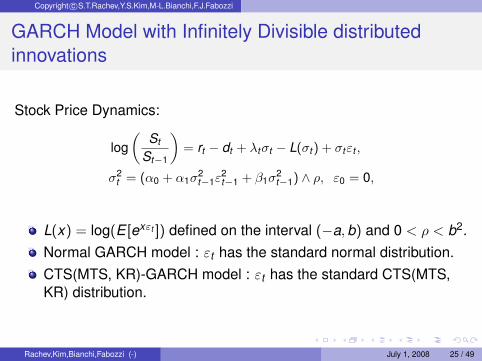
GARCH Model with Infinitely Divisible distributedinnovations

Stock Price Dynamics:

log(

St

St−1

)= rt − dt + λtσt − L(σt ) + σtεt ,

σ2t = (α0 + α1σ

2t−1ε

2t−1 + β1σ

2t−1) ∧ ρ, ε0 = 0,

L(x) = log(E [exεt ]) defined on the interval (−a,b) and 0 < ρ < b2.Normal GARCH model : εt has the standard normal distribution.CTS(MTS, KR)-GARCH model : εt has the standard CTS(MTS,KR) distribution.



Historical parameter estimation

Table: Statistic of the goodness of fit tests

Ticker Model KS(p-value) χ2(p-value) ADSPX normal-GARCH 0.0311 (0.0158) 323.4665 (0.4979) 401.9810

CTS-GARCH 0.0278 (0.0414) 304.2689 (0.6123) 0.6835MTS-GARCH 0.0276 (0.0436) 310.1418 (0.5191) 0.7354KR-GARCH 0.0277 (0.0426) 307.9739 (0.5378) 0.0595

IBM normal-GARCH 0.0547 (0.0000) 413.5590 (0.0000) 52009.9121CTS-GARCH 0.0223 (0.1656) 262.0601 (0.1462) 0.4819MTS-GARCH 0.0194 (0.3022) 237.5442 (0.4595) 0.5646KR-GARCH 0.0217 (0.1892) 262.2524 (0.1248) 0.0459

INTC normal-GARCH 0.0239 (0.1150) 352.4107 (0.0003) 133934.5383CTS-GARCH 0.0221 (0.1746) 300.8394 (0.0169) 0.3973MTS-GARCH 0.0221 (0.1718) 307.0700 (0.0090) 0.3715KR-GARCH 0.0220 (0.1765) 299.7535 (0.0152) 0.0496

MSFT normal-GARCH 0.0330 (0.0086) 329.1551 (0.0009) 12223.5241CTS-GARCH 0.0143 (0.6838) 226.5456 (0.6761) 0.9734MTS-GARCH 0.0149 (0.6331) 229.7076 (0.6383) 1.2923KR-GARCH 0.0121 (0.8558) 227.6621 (0.6222) 0.0540

AMZN normal-GARCH 0.0894 (0.0000) 367.7290 (0.0000) 204.7783CTS-GARCH 0.0222 (0.5718) 181.5525 (0.1791) 0.3310MTS-GARCH 0.0181 (0.8090) 176.6796 (0.2531) 0.3729KR-GARCH 0.0213 (0.6229) 178.3598 (0.1943) 0.0583



Normal-GARCH vs TS-GARCH

Normal

−3 −2 −1 0 1 2 3

−3

−2

−1

0

1

2

3

MTS

−3 −2 −1 0 1 2 3

−3

−2

−1

0

1

2

3

Data : Daily return for IBM



Normal-GARCH vs TS-GARCH

CTS

−3 −2 −1 0 1 2 3

−3

−2

−1

0

1

2

3

KR

−3 −2 −1 0 1 2 3

−3

−2

−1

0

1

2

3



Option prices

Call prices (March 10, 2006) with multi-maturities1. Normal-GARCH

1150 1200 1250 1300 1350 14000

20

40

60

80

100

120

140

3. KR-GARCH

1150 1200 1250 1300 1350 14000

20

40

60

80

100

120

140

2. CTS-GARCH

1150 1200 1250 1300 1350 14000

20

40

60

80

100

120

140



Implied volatility

Errors between the market and model prices[Time to maturity : 1 week, date : March 10, 2006]

APE AAE RMSE ARPENormal-GARCH 0.014214 0.47237 0.60438 0.27075CTS-GARCH 0.014994 0.49829 0.62068 0.30319KR-GARCH 0.0098485 0.3273 0.38034 0.28453

0.9 0.95 1 1.05 1.1 1.150.05

0.1

0.15

0.2

0.25

0.3

0.35

0.4

moneyness(K/S0)

impli

ed vo

latilit

y

marketNormal−GARCHCTS−GARCHKR−GARCH



Portfolio Optimization



Portfolio optimization

A realistic model for portfolio optimization has to consider someempirical facts:

volatility clustering ARMA-GARCH modelsheavy tails and skewness ⇒ TS distributions

tail dependence t-copula⇓

TS simulationt-copula fitting and simulation

optimization








optimization








optimization



Mean-Risk analysis

minw

ρ(rp)

subject to w ′e = 1w ′µ ≥ Rw ≥ 0

w vector of portfolio weightsρ is a risk measureR is a lower bound for the expected portfolio returnµ is the vector of stocks expected returns and e = (1, ..,1)

When ρ is the variance, we have the classic Markowitz mean-varianceproblem



Mean-Risk analysis

minw

ρ(rp)


w vector of portfolio weightsρ is a risk measureR is a lower bound for the expected portfolio returnµ is the vector of stocks expected returns and e = (1, ..,1)

When ρ is the variance, we have the classic Markowitz mean-varianceproblem



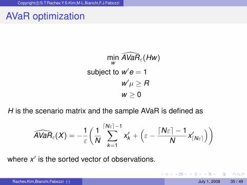
AVaR optimization

AVaRε(X ) :=1ε

∫ ε

0VaRp(X )dp

Why AVaR?coherent risk measureconsistent with the preference relations of risk-averse investorsan informed view of losses beyond VaRconvex and smooth function of portfolio weights



AVaR optimization

minw

AVaRε(Hw)


H is the scenario matrix and the sample AVaR is defined as

AVaRε(X ) = −1ε

(1N

dNεe−1∑k=1

x ′k +(ε− dNεe − 1

Nx ′dNεe

))where x ′ is the sorted vector of observations.



Asymmetric skewed t-copula

A multivariate skewed Student’s t distribution X with degree of freedomν is defined by means of the following stochastic representation

X = µ+ γW + Z√

W (1)

where µ ∈ Rd is a location vector, γ ∈ Rd is a vector accounting for theskewness, W ∼ IG(ν/2, ν/2) and Z ∼ N(0,Σ) is independent to W .

The stochastic representation (1) facilitates scenario generationan attractive model in higher dimensionstail dependence and asymmetric dependence



Simulating TS distributions

A CGMY process {Xt}[0,T ] with parameters (C, G, M, Y , 0) can besimulated by

Xtd=∞∑

j=1

[(Y Γj

2C

)−1/Y

∧ EjU1/Yj |Vj |−1

]Vj

|Vj |I{U′j≤t} + tbT t ∈ [0,T ],

{U ′j } ∼ U(0,T ), {Uj} ∼ U(0,1),{Ej} and {E ′j } ∼ Exp(1), {Γj} = E ′1 + . . .+ E ′j ,

{Vj} with P(Vj = −G) = P(Vj = M) = 12

0 < Y < 2, ‖σ‖ = 2C and bT ∈ R{Uj}, {Ej}, {E ′j }, {U ′j } and {Vj} are mutually independent.



Simulating TS distributions

0 0.2 0.4 0.6 0.8 1−5

0

5

10

15

20

KRCGMYα−stable



Implemented algorithm

Step 0 - data set

478 companies included in the S&P 500 index (daily data)time window from 12 March 2003 to 12 March 2008back-testing time period is 4 years from 12 March 2004 to 12March 2008




Step 1We reduce the dimensionality of the problem by modelling stockreturns with a multi factor linear model

Xi = αi +K∑

j=1

βi,jFj + εi

where factors are give by the PCA. Furthermore, we estimateparameters αi and βi,j .




PCA factors

0 50 100 150 200 250 300−0.8

−0.6

−0.4

−0.2

0

0.2

0.4

0.6

0.8

1




Step 2We model separately the univariate time-series

εi,t = ri,t − αi −K∑

j=1

βi,jFj,t

with αi , βi,j and εi,t estimated in the previous step. We assumethat time series εi,t , 1 ≤ t ≤ T follow an ARMA(1,1)-GARCH(1,1)dynamic with a stdCGMY noise and calibrate the model.




Step 3We assume that marginals of the multivariate time-series of factorreturns

(Fj,t )1≤j≤K ,1≤t≤T

follow an ARMA(1,1)-GARCH(1,1) dynamic with a stdCGMY noiseand calibrate each single one dimensional factor. Moreover, thedependence structure is also modelled by a skewed T-copula andcalibrated as well.




Step 4The scenarios matrix H is generated by 10.000 Monte Carlosimulations and the AVaR optimization problem is solved with R =6 mo U.S. Treasury + 5%

Step 5We rebalance the portfolio by moving the time window of 6 monthsand we repeat from Step 1 to Step 4 for a total of 8 times until thelast period from 12 September 2006 to 12 September 2007.

Step 6Then, we compare the performance of our optimal portfolio withthe S&P500 index and with an investment in the 6 months U.S.Treasury.



Results

0 200 400 600 800 1000 12001000

1100

1200

1300

1400

1500

1600

1700

1800

1900

days

valu

e in

$

S&P500AVaR portfolio6 months U.S. Treasury

Average number of holdings = 85



Ex post analysis

Sharpe ratio

SR(w) =w ′Er − rf

σp

S&P500 AVaR1 0.0453 0.51852 1.1884 2.03873 0.2710 1.28294 0.3377 1.34865 0.0095 0.32356 0.9673 1.33137 0.3010 -0.03288 -1.1418 -1.5320



Ex post analysis

Stable tail-adjusted return ratio

STARRε(w) =w ′Er − rf

AVaRε(w ′r)

S&P500 AVaR1 0.0218 0.21532 0.6353 1.01543 0.1396 0.64254 0.1628 0.63445 0.0046 0.15936 0.3810 0.54547 0.1238 -0.01338 -0.5212 -0.7156



Further improvements

increase the number of rebalancing times (each month, eachweek...)consider realistic constrains (transaction costs, turnover, numberof holdings,...)comparison by using different distributional hypothesis (KR,MTS,...)



S. Demarta and A.J. McNeil.The t Copula and Related Copulas.International Statistical Review, 73(1):111–129, 2005.

P. Embrechts, F. Lindskog, and A. McNeil.Modelling Dependence with Copulas and applications to risk management.In S.T. Rachev, editor, Handbook of heavy-tailed distributions in finance, pages 329–384, 2003.

Y. S. Kim, S. T. Rachev, M. L. Bianchi, and F. J. Fabozzi.A new tempered stable distribution and its application to finance.In Bol G., Rachev S. T., and Wuerth R., editors, Risk Assessment: Decisions in Banking and Finance, pages 51–84.Physika Verlag, Springer, 2008.

Y. S. Kim, S. T. Rachev, M. L. Bianchi, and F. J. Fabozzi.Financial market models with lévy processes and time-varying volatility.Journal of Banking and Finance, 32(7):1363–1378, 2008.

S.T. Rachev.Handbook of Heavy Tailed Distributions in Finance.Elsevier, 2003.

S.T. Rachev and S. Mittnik.Stable Paretian Models in Finance.Wiley New York, 2000.

S.T. Rachev, S. Mittnik, F.J. Fabozzi, S.M. Focardi, and T. Jašic.Financial Econometrics: From Basics to Advanced Modeling Techniques.The Frank J. Fabozzi series. Wiley, 2007.

S.T. Rachev, S.V. Stoyan, and F.J. Fabozzi.Advanced Stochastic Models, Risk Assessment, and Portfolio Optimization: The Ideal Risk, Uncertainty, and PerformanceMeasures.The Frank J. Fabozzi series. Wiley, 2008.


Documents

Market Crashes and Modeling Volatile Markets