Model and analysis of chemotactic bacterial patterns in a liquid medium

J. Math. Biol. (1999) 38: 359—375

Model and analysis of chemotactic bacterial patternsin a liquid medium

Rebecca Tyson1, S. R. Lubkin2, J. D. Murray3

1Department of Applied Mathematics, Box 352420, University of Washington, Seattle,WA 98195-2420, USA ([email protected])2Biomathematics Program, Box 8203, North Carolina State University, Raleigh,NC 27695-8203, USA ([email protected])3Department of Applied Mathematics, Box 352420, University of Washington, Seattle,WA 98195-2420, USA ([email protected]).

Received: 10 March 1998 /Revised version: 7 June 1998

Abstract. A variety of spatial patterns are formed chemotactically bythe bacteria Escherichia coli and Salmonella typhimurium. We focus inthis paper on patterns formed by E. coli and S. typhimurium in liquidmedium experiments. The dynamics of the bacteria, nutrient andchemoattractant are modeled mathematically and give rise to a nonlin-ear partial differential equation system.

We present a simple and intuitively revealing analysis of the pat-terns generated by our model. Patterns arise from disturbances toa spatially uniform solution state. A linear analysis gives rise toa second order ordinary differential equation for the amplitude of eachmode present in the initial disturbance. An exact solution to thisequation can be obtained, but a more intuitive understanding of thesolutions can be obtained by considering the rate of growth of indi-vidual modes over small time intervals.

Key words: Chemotaxis — Partial differential equations — Bacteria— Mathematical Modeling — Pattern formation

Introduction

In this paper we present a simple and intuitively revealing mathemat-ical analysis of transient solutions to a chemotaxis model involvingpartial differential equations. Our model equations are motivated byexperiments performed by Budrene and Berg [3], in which they

observed patterns formed by Escherichia coli and Salmonellatyphimurium. When placed in a liquid medium and exposed to inter-mediates of the tricarboxylic acid (TCA) cycle, the bacteria arrangethemselves into high density aggregates. The patterns appear, rear-range and eventually fade on a time scale which is short compared withthe generation time of the bacteria.

The simplest patterns are produced when the liquid medium con-tains a uniform distribution of bacteria and TCA cycle intermediate. Ofthe latter, succinate and fumarate produced the strongest effect. Onlya small amount is necessary, as the bacteria are merely exposed to theTCA cycle intermediate as a stimulant, and do not rely on it asa carbon source. The initially uniform distribution of bacteria begins toform a stranded pattern of higher-density regions. Subsequently, thepattern resolves into discrete clumps of roughly uniform size over theentire surface of the liquid, though the pattern often starts in onegeneral area and spreads from there. Over time the aggregates coalesce,thus becoming larger and decreasing in number. Ultimately the patterndissipates and cannot be induced to re-form.

Fluid dynamic convection cells are not believed to be responsiblefor these patterns (H. C. Berg, personal communication); we hypothe-size instead a primarily chemotactic mechanism. It is known that thebacteria secrete aspartate, a potent chemoattractant, in response to thestimulant. A chemoattractant is a chemical which the cells seek, inthe sense that they move up gradients of that chemical. This processtends to increase the local cell density, while diffusion tends to do theopposite. The competition between the two processes is the drivingforce behind the patterns observed. Thus the main players in theexperiments are the cells, the stimulant (succinate or fumarate) and thechemoattractant (aspartate).

The disappearance of the pattern is thought to be due to saturationof the chemotactic response. Since cellular production of chemoattrac-tant is not countered by any form of chemoattractant degradation (orinhibition), the amount of chemoattractant in the dish increases con-tinuously. As a result, the chemotactic response eventually saturates,and diffusion dominates.

We represent the experiments mathematically as a reaction-diffusion chemotaxis model. The numerical and analytic solutions ofthe equations verify our interpretation of the experimental results.

1 The model: a perturbation approach

Careful study of these experiments [3] has revealed that the biologicalprocesses most crucial in the formation of these bacterial patterns are

360 R. Tyson et al.

random migration and chemotaxis of bacteria. Also playing an impor-tant role is production of chemoattractant. There is no growth or deathof cells over the brief time course of the liquid experiments, nor is thereany uptake of aspartate by the cells as the liquid medium containssufficient nutrient for the cells from other sources (E. O. Budrene,personal communication). We thus formulate a model consisting oftwo conservation equations

LnLt

"Dn+2n!+ ·C

k1n

(k2#c)2

+cD(1)

LcLt

"Dc+2c#k

3s

k4n2

k9#n2

.

The variables n, c and s represent cell density, chemoattractant concen-tration, and nutrient concentration respectively. There is no equationfor the nutrient in these experiments since so little of the nutrient isconsumed. Thus, s is a parameter in this study. The terms on the righthand side represent, in order left to right and top to bottom, randomand chemotactic cellular motion, chemoattractant diffusion, andchemoattractant production.

These equations are discussed in detail in [11]. We summarize themain points here. E. coli and S. typhimurium have been studied in detailand experimental results are available to aid in the selection of func-tional forms for the terms in equation (1). Diffusion coefficients for therandom migration of cells [1, 2, 10] and chemotactic flux [5—7] havebeen measured by a number of researchers. For aspartate production,succinate is necessary, and the amount produced increases with theamount of succinate present [4]. Analysis of the parent model to thecurrent one [11] shows that the production of aspartate must increasesufficiently quickly at low succinate concentrations. It must also satu-rate however, since the cells do not have unlimited capacity to produceaspartate, Thus, guided by the experimental data, we arrive at themathematical model (in dimensionless form)

LuLt

"du+2u!a+ · C

u(1#v)2

+vD(2)

LvLt

"+2v#wu2

k#u2

where u, v and w represent cell density, chemoattractant concentrationand succinate concentration respectively. In this paper we focus on theexperiments where succinate is initially uniformly distributed and not

Model and analysis of chemotactic bacterial patterns in a liquid medium 361

consumed. In this case w is constant. For our model analysis, presentedbelow, we consider the one-dimensional situation, and generalise totwo dimensions numerically. Zero flux boundary conditions are usedthroughout, in order to make the analysis and simulations consistentwith the experiment.

The absence of growth and death in the cell population (over thetime course of the experiment) gives the conservation equation

Pl

0

u (x, t) dx"u0l"l,

where uois the average initial nondimensional cell density. The param-

eter values are listed in Table 1 (dimensional) and Table 2 (dimensiona-less). The parameter k is unknown to us. The ratio of dimensionlesstime to dimensional time is unknown, by the Buckingham Pi theorem.The initial conditions of the experiment are uniform nonzero celldensity and zero concentration of chemoattractant. So, from the non-dimensionalization we have

u(x, 0)" 1 and v(x, 0)"0.

Table 1. Known and estimated dimensional parameter values used in equations (1)

Parameter Value Source

k1

3.9]10~9Mcm2s~1 Dahlquist, Lovely and Koshland, 1972k2

5]10~6M Dahlquist, Lovely and Koshland, 1972k3

Unknownk4

Unknownk9

UnknownD

n2—4]10~6 cm2 s~1 Berg and Turner, 1990; Berg, 1983 p93

Dc

8.9]10~6 cm2 s~1 Berg 1983D

s+9]10~6 cm2 s~1 Berg 1983

n0

108 cellsml~1 Budrene and Berg, 1991s0

1—3]10~3M Budrene and Berg, 1995

Table 2. Known and estimated values for the dimensionless variables and parametersused in the study of the E. coli and S. typhimurium model, equations (2)

Variable Initial value Parameter Value

u0

1.0 a 80—90w0

1.0 du

0.25—0.5v0

0.0 k Unknown

362 R. Tyson et al.

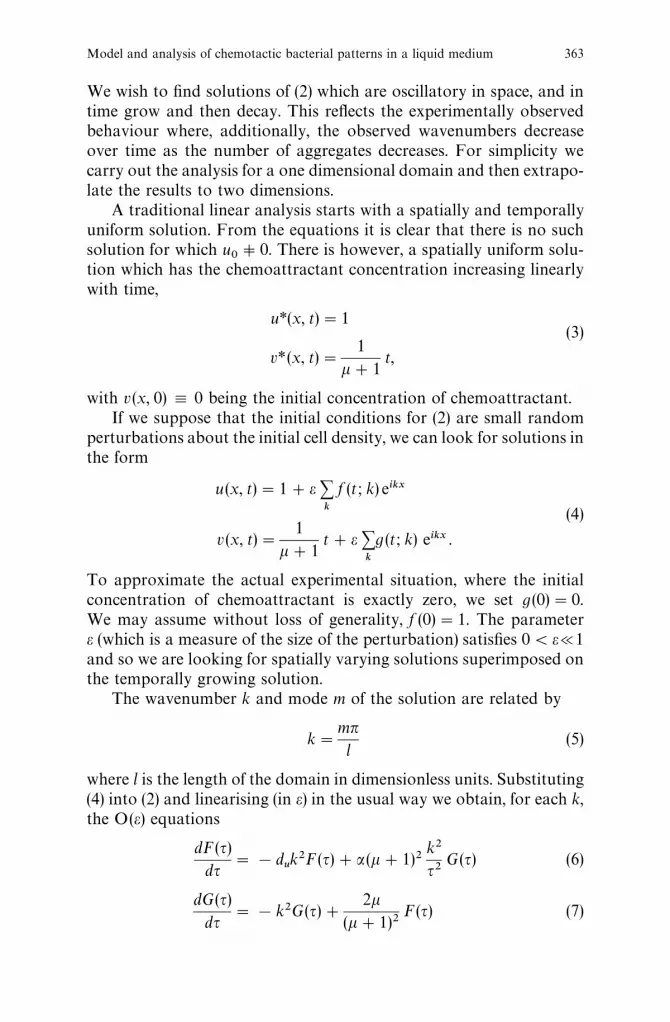
We wish to find solutions of (2) which are oscillatory in space, and intime grow and then decay. This reflects the experimentally observedbehaviour where, additionally, the observed wavenumbers decreaseover time as the number of aggregates decreases. For simplicity wecarry out the analysis for a one dimensional domain and then extrapo-late the results to two dimensions.

A traditional linear analysis starts with a spatially and temporallyuniform solution. From the equations it is clear that there is no suchsolution for which u

090. There is however, a spatially uniform solu-

tion which has the chemoattractant concentration increasing linearlywith time,

u*(x, t)"1(3)

v*(x, t)"1

k#1t,

with v (x, 0),0 being the initial concentration of chemoattractant.If we suppose that the initial conditions for (2) are small random

perturbations about the initial cell density, we can look for solutions inthe form

u (x, t)"1#e +k

f (t ; k) eikx

(4)

v (x, t)"1

k#1t#e +

k

g (t ; k) eikx .

To approximate the actual experimental situation, where the initialconcentration of chemoattractant is exactly zero, we set g(0)"0.We may assume without loss of generality, f (0)"1. The parametere (which is a measure of the size of the perturbation) satisfies 0(e@1and so we are looking for spatially varying solutions superimposed onthe temporally growing solution.

The wavenumber k and mode m of the solution are related by

k"mnl

(5)

where l is the length of the domain in dimensionless units. Substituting(4) into (2) and linearising (in e) in the usual way we obtain, for each k,the O(e) equations

dF(q)dq

"!duk2F(q)#a (k#1)2

k2

q2G(q) (6)

dG(q)dq

"!k2G(q)#2k

(k#1)2F(q) (7)


where q"k#1#t (note that q0"k#1'0) and for a given k,

F(q),f (t ; k), G(q),g(t ; k). The coefficient of the second term on theright hand side of (6) is the only one which depends on the chemotaxisparameter a.

It is clear from (6) that as qPR the coefficient of G (q) tends tozero, and the solution for F(q) reduces to a decaying exponential. Oncethis happens, the solution of (7) also gives a decaying exponential. So,with the forms (4) the mechanism accounts for ultimate pattern dis-appearance with time. This is also consistent with the original equa-tions (2). Since the cells do not die (no death term in the first equation)and since the chemoattractant is produced but never degraded (nodegradation term in the second equation), the chemoattractant concen-tration should continually increase. Thus, since the chemotaxis term isonly large when v, the chemoattractant concentration, is small, theeffect of chemotaxis will continually decrease until diffusion dominates.Let us now consider the temporary growth of spatial pattern from theinitial disturbance.

For q near q0

more insight can be gained by combining equations(6) and (7) to create a single second order differential equation for theamplitude of the cell density pattern, F(q):

d2Fdq2

#k2 A(du#1)#2q B

dFdq

#k2 Aduk2#2d

uq

!

2akq2 B F"0 (8)

This equation has an exact solution in terms of hypergeometricfunctions

F(q)"e~(1`A)q`Cln(q)2 q1`B

2 CK2H

U AC2A

#

1#B2

, 1#B, AqB#K

1H

1F1 AC2A

#

1#B2

, 1#B, AqBDwhere

A"k2 Ddu!1 D

B"J1#8akk2

C"2k2(k2(du#1)!2d

u)

.

The special functions HU

and H1F1

are the confluent hypergeometricfunction and the Kummer confluent hypergeometric function respec-tively. This exact solution is not intuitively revealing, and so we useother approaches to obtain a clear understanding of the solution F(q).

364 R. Tyson et al.

2 An analytic approximation

To begin the analysis, we make the assumption that the coefficients ofthe second order ordinary differential equation (8) change much lessrapidly than the function itself and its derivatives. This lets us compare(8) to a constant coefficient second order equation over small intervalsof q. Denoting the coefficients of (8) by D (q) and N(q) we obtain

d2Fdq2

#D(q)dFdq

#N (q) F"0 (9)

where

N(q)"k2Aduk2#2d

uq

!

2akq2 B (10)

D(q)"k2 A(du#1)#2qB. (11)

The last term in the bracketed expression in (10) is the only one inwhich a appears. The parameter k appears explicitly only in that sameterm, but is also contained in the expression for q and so its effect is notso easily isolated. Note that D(q) is positive for all times q greater thanq0, while N(q) can be positive, negative or zero for q near q

0. For all

q sufficiently large, N(q)'0. Considering N(q) and D (q) constant forthe moment, the solution of (9) over any sufficiently small q intervals isof the form

FI (q)"k1ej`q#k

2ej~q

where

j$"1

2(!D(q)$JD (q)2!4N(q)) (12)

Since D(q)'0 ∀q, we have Re(j~

)(0 ∀q. The sign of Re(j`) can

vary however, and depends on the sign of N(q). When N(q)(0 forsome k2, Re(j

`)'0 and the amplitude of that mode grows.

We focus our attention on how the chemotaxis coefficient a and thewavenumber k alter the solutions. If a is sufficiently large then N(q)will be negative for small values of q, including q

0. As q increases, N(q)

will increase through zero and become positive. The effect on j`

is tomake the real part of the eigenvalue positive for small q and negativefor large q. The point q

#3*5at which j

`passes through zero is the same

point at whichN(q) becomes zero. Thus, for small q, one component ofFI is a growing exponential, while for larger q both exponentials aredecaying. We predict then, that a has a destabilising influence, that is,the growth of pattern becomes more likely as a increases.


For sufficiently large k2, N(q) becomes positive for all q, resulting insolutions which are strictly decaying. Thus we would not expect to seewavenumbers larger than K, where

K2"2

du(1#k) A

ak1#k

!duB (13)

is found by solving N (q0)"0. As time advances, fewer and fewer

modes remain unstable, and as qPR, the only unstable modes arethose in a diminishing neighbourhood of 0. We can determine thefastest-growing wavenumber, K

'308, at any time by setting

j`

(k2)"0,N(q)"0 and solving for k2 . This gives

K2'308

"

2q A

akduq!1B

which decreases with time. Thus we would not expect any wavenumberlarger than K

'308to dominate the solution.

If our constant coefficient assumption is approximately correctover small but finite intervals of q, then a series of solutions FI com-puted in sequential intervals *q could give rise to a solution whichincreases to a maximum and then decreases for all subsequent q. Theincreasing portion would occur while j

`is positive. When we compute

a numerical solution of the equation, we obtain the expected behaviour(Fig. 1). To obtain the numerical solution, we used the NAG stiff ODEsolver D02NBF with set up routines D02NSF and D02NVF. Thelatter is the integrator set-up routine for Backward DifferentiationFormulae.

We now construct an approximate analytic form for F(q). The truelocation q"q

#3*5of the maximum value of F(q), F

.!9, may be close to

q8#3*5

, where

N (q8#3*5

)"0 8 q8#3*5

"

!1#J1#2akdu

k2

k2. (14)

We compare q8#3*5

with q#3*5

obtained numerically; the results are shownin Fig. 2. The dotted line corresponds to q8

#3*5which we can compute for

continuous values of k2. The circles correspond to the numericallycomputed q

#3*5at various values of k2. The comparison is very close,

and improves as k2 and a increase.The difference between q8

#3*5and q

#3*5gives an indication of the size of

d2F/dq2 at q#3*5

. By definition, q#3*5

is the time at which dF/dq"0 andso (9) reduces to

d2Fdq2 K q#3*5"!N (q

#3*5)F.

366 R. Tyson et al.

Fig. 1. The amplitude F(q) of the k"1.6 perturbation of the initial uniform celldensity. The other parameter values are: d

u"0.33, a"80, k"1, u

0"1, w"1 and

l"10

Fig. 2. Comparison of q#3*5

(circles) and q8#3*5

(predicted q#3*5

) (dotted line) plotted againstwavenumber. Parameter values are a"80, d

u"0.33, k"1, u

0"1, w"1 and l"10

Since the second derivative of a function is always less than zero ata maximum we know that N (q

#3*5) is positive. Thus q has already

increased past the point where N (q) changes sign, and q8#3*5

gives usa minimum estimate for q

#3*5. From Fig. 2 we see that q8

#3*5and q

#3*5are

reasonably close, which suggests that N(q#3*5

) may be close to zero. Inturn, this indicates that d2F/dq2 may be numerically small at themaximum, F

.!9.


We are thus encouraged to solve equation (9) with the secondderivative term omitted, and compare the approximate solution withthe numerical one. After some straightforward algebra we find thesolution of the first order ordinary differential equation to be

F1(q)"C

(du#1)k2q

0#2

(du#1)k2q#2 D

2akk22

!2du(du`1~2)(du`1)2

Cqq0D

2akk22

e dudu`1 k2(q0~q). (15)

Plots of the first order and second order equation solutions F(q) andF1(q) are shown in Fig. 3. For this figure a was set to 30, since the two

curves have such disparity in magnitude for a"80 that they cannot beviewed on the same coordinate grid. The observations below applyequally however, for the larger value of a.

At first glance we notice the marked difference in the height of thetwo functions. Apart from this difference however, the two functionshave many similarities: (1) the peaks occur at approximately the samevalue of q, (2) the peak interval, defined as the time during whichF(q)'F (q

0), is about the same, especially for the lower frequencies,

and (3) the two curves appear to be similarly skewed to the left.Increasing a results in a large increase in both F

.!9and F

1.!9, but

doesn’t change the slope. The two solutions are also similar withrespect to the behaviour of the different modes investigated. The largerthe value of k2, the earlier q

#3*5is reached, and the shorter the interval

over which F or F1

is larger than the initial value F0.

If we normalise the data for F(q) and F1(q) so that it lies in the

interval [0, 1] we see that the two solutions map almost directly on topof each other (Fig. 4). The main difference therefore, between theapproximate solution and the exact solution (obtained numerically) is

Fig. 3. F (q) (solid line) and F1(q) (dotted line) plotted together against q for a"30 and

various values of k. The other parameter values are as listed in Fig. 2

368 R. Tyson et al.

Fig. 4. The solutions F(q) (solid line) and F1(q) (dotted line) plotted against q and

normalised to lie between 0 and 1. The parameter values are as listed in Fig. 2

simply in a scaling factor. This scaling factor is very large, suggestingthat the second order derivative term is not small outside the neigh-bourhood of the maximum.

At this stage we have an intuitive understanding of the solutionsF(q) of equation (8). We also have an approximate analytic solution,F1(q), which we can use to predict the effect of changing various

parameters.

3 Interpretation of results

In terms of the model equations, we are particularly interested inpredicting the size and number of aggregates which will form, and thelength of time during which they will be visible, that is, when F(q) issufficiently large. If nonlinear effects are not too strong, we expect thatthe number of aggregates will be determined by the combined effect ofthe solutions corresponding to the various modes.

Numerical results are shown in Fig. 5. We observe that there is onewavenumber which attains a higher amplitude than any other. Werefer to this wavenumber as k

.!9(here k

.!9"2.20). We also note that

every wavenumber k larger than k.!9

initially has a slightly highergrowth rate than k

.!9. These high frequencies quickly begin decaying

however, while the amplitude of the k.!9

pattern is still growingrapidly.

Once the k.!9

solution begins to decay, solutions corresponding tosmaller wavenumbers become largest in decreasing order. The ampli-tude of each solution with k(k

.!9is always in the process of decaying,

once it supersedes the next highest mode. Thus we should see acontinuous decrease in the wavenumber of the observed pattern as


Fig. 5. F(q) for discrete values of k"mn/l, m"4 to 9 (or k"1.26 to 2.83). The m"9curve decays the fastest, then the m"8 curve, etc. The curve corresponding to m"7has the highest peak. The other parameter values are: d

u"0.33, a"80, k"1, u

0"1,

w"1 and l"10. (K"10.9)

t increases, accompanied by a decrease in amplitude. This correspondsto the biologically observed coalescing of aggregates and eventualdissipation of pattern. Note that for these figures K

'308"5.47 and so

k.!9

is less than K'308

by a factor of 2. For all of the numerical solutionsobserved in this study, k

.!9was consistently much less than K

'308.

4 Numerical simulation results

We can now compare the predictions of the linear theory with theactual solution behaviour of the partial differential equations. Simula-tion results were obtained using Strang Splitting and Clawpack [8, 9].The method and its behaviour is discussed in detail in Tyson et al. [12].For all of the simulations, zero flux boundary conditions were used.The initial condition in chemoattractant concentration is zero every-where on the domain, and in cell density is a random perturbationabout u

0"1. The random perturbation was obtained via the Fortran

random number generator routine, rand, which produces pseudo-random real numbers distributed uniformly over (0, 1). Various seeds

370 R. Tyson et al.

and grid refinements were used. The results presented in the figuresbelow are all generated from runs using the same seed, grid spacing(Dx"0.06) and noise amplitude (order 10~1).

A time sequence for a"80 is shown in Fig. 6. The sequence wastruncated at the time beyond which little change was observed in thenumber of peaks, and the pattern amplitude simply decreased. Theplots in the left hand column of each figure are the cell density profilesat various times q, while the plots in the right hand column are thecorresponding power spectral densities. The density axis for the latterplots are restricted to lie above the mean value of the initial powerspectral density, at q"q

0. This highlights the pattern modes which

grow.As predicted in equation (13), the power spectral density plots

indicate that spatial pattern modes with wavenumber higher thanK"10.9 do not grow. Also, spread of ‘‘nonzero’’ modes decreases astime increases. In the actual cell density distribution, the patternobserved initially has many peaks, and the number of these decreasesover time. Our prediction for the value of k

.!9is off by a factor of two

in these figures. The solution is actually dominated by k.!9

+1.1 whilethe predicted value was 2.2.

Moving to two dimensional simulations, we obtain the same typeof results from the model as was observed in the one dimensional case.An initial condition consisting of small random perturbations abouta uniform distribution of cells produces patterns consisting of a ran-dom arrangement of spots (Fig. 7). From the surface plot, Fig. 8, it isclear that the aggregates of cells are very dense in comparison to theregions in between. The number of spots is large at first and thendecreases over time as neighbouring spots coalesce. Eventually, all ofthe spots disappear.

Recall that this is exactly what is observed in the bacterial experi-ments. To begin with, bacteria are added to a petri dish containinga uniform concentration of succinate. The mixture is well-stirred, andthen allowed to rest. At this point, the state of the solution in the petridish is mimicked by the initial condition for our model: small perturba-tions of a uniform distribution of cells and succinate. After a shortperiod of time, on the order of 20 minutes, the live bacteria aggregateinto numerous small clumps which are very distinct from one another.This behaviour corresponds to the random arrangement of spotsseparated by regions of near-zero cell density observed in the modelsolutions. Experimentally, the bacterial aggregates are seen to jointogether, forming fewer and larger clumps. This also is present inthe mathematical model, and is clearly evident when the solutionsare displayed as a movie with the frames separated by small time


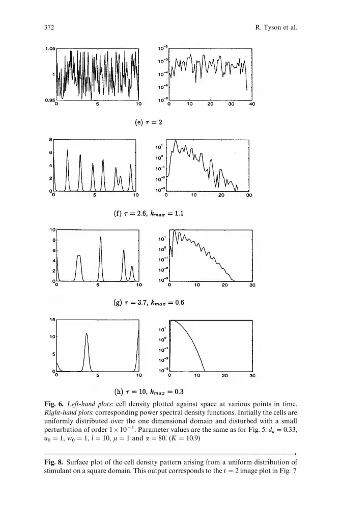
Fig. 6. ¸eft-hand plots: cell density plotted against space at various points in time.Right-hand plots: corresponding power spectral density functions. Initially the cells areuniformly distributed over the one dimensional domain and disturbed with a smallperturbation of order 1]10~1. Parameter values are the same as for Fig. 5: d

u"0.33,

u0"1, w

0"1, l"10, k"1 and a"80. (K"10.9)

&&&&&&&&&&&&&&&&&&&&&&&&&&&&&&&&&&&&"Fig. 8. Surface plot of the cell density pattern arising from a uniform distribution ofstimulant on a square domain. This output corresponds to the t"2 image plot in Fig. 7

372 R. Tyson et al.

Fig. 7. Two dimensional cell density pattern arising from a uniform distribution ofstimulant on a square domain. White corresponds to high cell density, black to low celldensity. Parameter values: d

u"0.33, a"80, k"1, u

0"1, w"1 and l"10


increments. In both the model and experiment, the spots eventuallydisappear and cannot be induced to re-form. This is explained by themathematical model as a saturation of the chemotactic response,which no longer has any effect as the production of chemoattractantincreases continually.

5 Conclusions

In this paper, we explored a simple and intuitively revealing analysiswhich explains how evolving patterns of randomly arranged spotsappear transiently in a chemotaxis model and in experiment. Thecentral idea is to consider the rate of growth of individual modesover small time intervals, and extrapolate from this to the combinedbehaviour of all disturbance frequencies. Low mode number per-turbations to the uniform solution are unstable and grow in magni-tude, but eventually these stabilize and decay with the larger modenumbers stabilizing first. This agrees qualitatively, and to a greatextent quantitatively, with what is observed experimentally and nu-merically: clumps form, coalesce into larger aggregates, and eventuallydisappear.

Acknowledgements. We thank Julian Cook for his helpful contributions to this project.This work has been supported in part by NSF grants DMS-9306108 (SRL) andDMS-9500766 (SRL, JDM), and by NSERC scholarships PGSA and PGSB (RT).

References

1. H. C. Berg and L. Turner. Chemotaxis of bacteria in glass capillary arrays.Biophys. J., 58: 919—930, 1990

2. Howard C. Berg. Random Walks in Biology. Princeton University Press, Prin-ceton, NJ, 1983

3. E. O. Budrene and H. C. Berg. Complex patterns formed by motile cells ofescherichia coli. Nature, 349(6310): 630—633, 1991

4. E. O. Budrene and H. C. Berg. Dynamics of formation of symmetrical patterns bychemotactic bacteria. Nature, 376 (6535): 49—53, 1995

5. F. W. Dahlquist, P. Lovely, and Koshland, Jr, D. E. Qualitative analysis ofbacterial migration in chemotaxis. Nat. New Biol., 236: 120—123, 1972

6. R. M. Ford and D. A. Lauffenburger. Analysis of chemotactic bacterial distribu-tions in population migration assays using a mathematical model applicable tosteep or shallow attractant gradients. Bulletin of Mathematical Biology, 53(5):721—749, 1991

7. R. Lapidus and R. Schiller. Model for the chemotactic response of a bacterialpopulation. Biophys. J., 16: 779—789, 1976

374 R. Tyson et al.

8. R. J. LeVeque. CLAWPACK software. available from netlib.att.com in net-lib/pdes/claw or on the Web at the URL http: //www.amath.washington. edu/&rjl/clawpack.html

9. R. J. LeVeque. CLAWPACK USER NOTES. available from netlib.bell-labs.comin netlib/pdes/claw/doc or at http://www.amath.washington.edu/&rjl/claw-pack.html

10. B. R. Phillips, J. A. Quinn, and H. Goldfine. Random motility of swimmingbacteria: Single cells compared to cell-populations. AIChE Journal, 40: 334—348,1994

11. R. Tyson, S. R. Lubkin, and J. D. Murray. A minimal mechanism of bacterialpattern formation. Proc. Roy. Soc. B (in press, 1999)

12. R. Tyson, L. G. Stern, and R. J. LeVeque. Fractional step methods applied toa chemotaxis model. Journal of Mathematical Biology (in press, 1999)


Documents

Model and analysis of chemotactic bacterial patterns in a liquid medium