Embed Size (px)
Citation preview
Modeling shallow water table evaporationin irrigated regions
Chuck Young & Wesley Wallender & Gerrit Schoups &Graham Fogg & Blaine Hanson & Thomas Harter &
Jan Hopmans & Richard Howitt & Ted Hsiao &
Sorab Panday & Ken Tanji & Susan Ustin & Kristen Ward
Published online: 30 May 2007# Springer Science + Business Media B.V. 2007
Abstract Groundwater discharge through evaporation due to a shallow water table can be animportant component of a regional scale water balance. Modeling this phenomenon inirrigated regions where soil moisture varies on short time scales is most accuratelyaccomplished using variably saturated modeling codes. However, the computational demandsof these models limit their application to field scale problems. The MODFLOW groundwatermodeling code is applicable to regional scale problems and it has an evapotranspirationpackage that can be used to estimate this form of discharge, however, the use of time-invariantparameters in this module result in evaporation rates that are a function of water table depthonly. This paper presents a calibration and validation of the previously developed MOD-HMSmodel code using lysimeter data. The model is then used to illustrate the dependence of baresoil evaporation rates on water table depth and soil moisture conditions. Finally, an approachfor estimating the time varying parameters for the MODFLOW evapotranspiration packageusing a 1-D variably saturated MOD-HMS model is presented.
Keywords Evaporation . Groundwater model . Shallowwater table
Irrig Drainage Syst (2007) 21:119–132DOI 10.1007/s10795-007-9024-4
C. Young (*)Stockholm Environment Institute, 133 D Street, Suite F Davis, CA 95618, USAe-mail: [email protected]
W. Wallender :G. Fogg : B. Hanson : T. Harter : J. Hopmans : T. Hsiao :K. Tanji : S. UstinDepartment of Land, Air, and Water Resources, U.C. Davis, One Shields Avenue, Davis,CA 95616, USA
G. SchoupsDepartment of Integrated Environmental Studies, Flemish Institute for Technological Research (VITO),Boeretang 200, 2400 Mol, Belgiume-mail: [email protected]
R. Howitt : K. WardDepartment of Agricultural and Resource Economics, U.C. Davis, One Shields Avenue, Davis,CA 95616, USA
S. PandayHydrogeologic Incorporated, 1155 Herndon Parkway, Suite 900, Herndon, VA 20170, USA
Introduction
Water that moves upwards through capillary rise from a shallow water table can enter theatmosphere through plant transpiration or direct evaporation from bare soil. On the onehand, this upward flux can be beneficial to agriculture from the standpoint of meeting cropwater requirements (Wallender et al. 1979; Eching et al. 1994), but on the other hand,salinity in the water can lead to crop damage and soil degradation (Gardner 1958; SJVDP1990). Ground water models representing regions with shallow water tables need to accountfor this important path of groundwater discharge (Belitz et al. 1993). Model codes such asMOD-HMS and HYDRUS calculate variably saturated flow and bare soil evaporationusing the Richards Equation (Panday and Huyakorn 2004; Simunek et al. 1998), however,their application to regional problems is constrained by computational demands. In contrast,the MODFLOW groundwater modeling code (MacDonald and Harbaugh 1988; Banta2000) can be applied to regional problems. It includes a simplified representation ofgroundwater discharge through capillary rise from the water table.
In regional scale modeling efforts using MODFLOW, evapotranspiration from irrigatedlands is often calculated in a pre-processing step using climatic data and published cropcoefficients (Allen et al. 1998), however, the effects of a shallow water table are notconsidered in this approach. This leaves a model designer with the need to account forgroundwater discharge in the form of bare soil evaporation that is not calculated usingclimatic data and crop coefficients. One approach is to use crop coefficients and climaticdata to estimate plant transpiration and the bare soil evaporation associated with irrigation.Evaporation caused by the presence of a shallow water table is then calculated using theevapotranspiration package. A potential problem with this approach is the lack of accountingfor soil moisture between the water table and the ground surface. In irrigated regions wheresoil moisture varies on a daily or hourly time scale, this can lead to poor estimates of baresoil evaporation. One solution to this problem is the use of detailed, 1-D, MOD-HMS orHYDRUS models to calculate parameters for the regional scale MODFLOW model.
The objectives of this paper are to illustrate the effect of a shallow water table on baresoil evaporation rates in a transient irrigated setting and provide a method for utilizing avariably saturated model code to inform the parameterization of the evapotranspirationpackage in MODFLOW. The first part describes MOD-HMS and its approach to modelingflow in the unsaturated zone including bare soil evaporation. The second part is adescription of the first calibration and validation of the MOD-HMS bare soil evaporationmodule using lysimeter data. The third part presents an approach to the parameterization ofthe evapotranspiration package in MODFLOW using the results of a MOD-HMS model.
Background
Studies of capillary rise from the water table have centered on steady state analyticalsolutions, transient state analytical solutions, and lysimeter experimental studies. Steadystate analytical solutions have their origins in the work of Gardner and Fireman (1958) andGardner (1958). The solutions presented describe steady state vertical upward flow from thewater table to a bare soil surface. The authors reported the upward flux was limited by theatmospheric evaporative potential when the water table was shallow. With deeper watertables, soil physical properties limited upward flow. Gardner (1958) also describes thecontribution of the vapor phase to overall evaporation. It was concluded that subsurfacevapor movement would seldom exceed 20% of maximum liquid transport and would
120 Irrig Drainage Syst (2007) 21:119–132
usually be much less. More recent research has reinforced this conclusion by finding thatliquid water movement deeper in the soil limits total evaporation on daily or greater timescales (Saravanapavan and Salvucci 2000). Transient analytical models have beendeveloped to study the role of capillary rise in soil salinization (Jorenush and Sepaskhah2003; Prathapar et al. 1992). These models cannot describe how much of capillary risewater goes to bare soil evaporation versus transpiration. Lysimeter studies (Yang et al.2000; Soppe and Ayars 2003) also cannot separate the paths of capillary rise water.
In MODFLOW 2000, evapotranspiration is treated as a head-dependant flux boundary.The functional relationship between water table depth and evapotranspiration rate isexpressed using line segments. This is an improvement over the original evapotranspirationpackage in MODFLOW in which the user could only specify the maximum rate, itsassociated elevation (ET surface) and the extinction depth. For water table elevationsbetween the evaporating surface and the extinction depth, the evaporation rate variedlinearly between the maximum rate and zero. In MODFLOW 2000, for water table depthsbetween the ET surface and the extinction depth, the evaporation rate varies linearly withinuser specified segments. This allows the user to specify a more realistic exponential curveshape for the functional relationship.
Numerical model
MOD-HMS, created by HydroGeologic Inc. (Panday and Huyakorn 2004), was used for thenumerical experiments described in this paper. MOD-HMS is a modified version ofMODFLOW (McDonald and Harbaugh 1988), the widely used finite differencegroundwater modeling code created by the USGS. The modifications allow the user tosolve a single equation representing Richard’s Equation in the unsaturated zone andgroundwater flow in the saturated region.
@
@xKxxkrw
@h
@x
� �þ @
@yKyykrw
@h
@y
� �þ @
@zKzzkrw
@h
@z
� ��W ¼ φ
@Sw@t
þ SwSs@h
@tð1Þ
where:
x, y, and z are Cartesian coordinates (L);Kxx, Kyy, andKzz
are the components of the hydraulic conductivity tensor in the x, y, and zdirections (L/T);
krw is the relative permeability which is a function of water saturation;h is the total hydraulic head (L);W represents sinks and/or sources (T−1);φ is the porosity;Sw is the degree of saturation which is a function of pressure head;Ss is the specific storage of the porous material (L−1); andt is time (T).
When a model cell is fully saturated Sw=1.0, krw=1.0, and Equation 1 reduces to thegroundwater flow equation:
@
@xKxx
@h
@x
� �þ @
@yKyy
@h
@y
� �þ @
@zKzz
@h
@z
� ��W ¼ Ss
@h
@tð2Þ
Irrig Drainage Syst (2007) 21:119–132 121
In addition to the parameters specified above, the relationships between effective watersaturation, pressure head, and relative permeability must be specified. MOD-HMS representsthe relative saturation – pressure head relationship using the van Genuchten parameters.
Se ¼ Sw � Swr1� Swr
¼ 1
1þ ahp� �bh ig ð3Þ
where:
Se is effective water saturation;Swr is residual water saturation;hp is pressure head defined as the negative of (h–z) with z as the vertical upward
coordinate (L);α, β, andγ
are the van Genuchten parameters with γ=1–1/β.
Relative permeability is related to effective water saturation through:
krw ¼ S1=2e 1� 1� S1=γe
� �γh i2ð4Þ
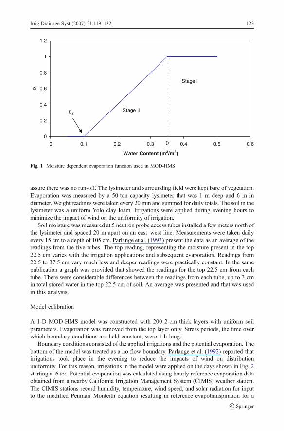
The evaporation algorithm is based on the two-stage evaporation concept (Ritchie 1972).During the first stage, evaporation is limited by available energy at the ground surface. DuringStage II the soil has dried to the point that unsaturated hydraulic conductivity limits theevaporation rate as water is transported up through the soil profile in response to the hydraulicgradient. The evaporation is a flux boundary calculated as a function of water content:
ESI ¼ aI Ep
� �EDFI ð5Þ
where
ESI is evaporation from bare soil in model layer I (L/T)Ep is the evaporative potential (L/T)EDFI is the evaporation distribution function over the model layers, the sum of EDFI over
all layers is 1αI is a piece-wise linear function that reduces the evaporation rate as a function of
water content within layer I (Fig. 1).
The function shown in Fig. 1 reduces the evaporation rate linearly from the user specified,layer specific values of θ1 to θ2 (Stage II). At water contents greater than θ1 (Stage I),evaporation from layer I is removed at the potential rate (Ep×EDFI). For water contentvalues less than θ2 no water is removed.
Calibration and validation of model
Field experiment
Field data were obtained from lysimeter experiments described by Parlange and others (Katuland Parlange 1992; Parlange et al. 1992, 1993). The experiments were carried out fromSeptember 4 to December 12, 1990 at the University of California at Davis experimentalfarm. During that time 14 sprinkler irrigations were applied at a rate no greater than 0.5 cm/h to
122 Irrig Drainage Syst (2007) 21:119–132
assure there was no run-off. The lysimeter and surrounding field were kept bare of vegetation.Evaporation was measured by a 50-ton capacity lysimeter that was 1 m deep and 6 m indiameter. Weight readings were taken every 20 min and summed for daily totals. The soil in thelysimeter was a uniform Yolo clay loam. Irrigations were applied during evening hours tominimize the impact of wind on the uniformity of irrigation.
Soil moisture was measured at 5 neutron probe access tubes installed a few meters north ofthe lysimeter and spaced 20 m apart on an east–west line. Measurements were taken dailyevery 15 cm to a depth of 105 cm. Parlange et al. (1993) present the data as an average of thereadings from the five tubes. The top reading, representing the moisture present in the top22.5 cm varies with the irrigation applications and subsequent evaporation. Readings from22.5 to 37.5 cm vary much less and deeper readings were practically constant. In the samepublication a graph was provided that showed the readings for the top 22.5 cm from eachtube. There were considerable differences between the readings from each tube, up to 3 cmin total stored water in the top 22.5 cm of soil. An average was presented and that was usedin this analysis.
Model calibration
A 1-D MOD-HMS model was constructed with 200 2-cm thick layers with uniform soilparameters. Evaporation was removed from the top layer only. Stress periods, the time overwhich boundary conditions are held constant, were 1 h long.
Boundary conditions consisted of the applied irrigations and the potential evaporation. Thebottom of the model was treated as a no-flow boundary. Parlange et al. (1992) reported thatirrigations took place in the evening to reduce the impacts of wind on distributionuniformity. For this reason, irrigations in the model were applied on the days shown in Fig. 2starting at 6 PM. Potential evaporation was calculated using hourly reference evaporation dataobtained from a nearby California Irrigation Management System (CIMIS) weather station.The CIMIS stations record humidity, temperature, wind speed, and solar radiation for inputto the modified Penman–Monteith equation resulting in reference evapotranspiration for a
0
0.2
0.4
0.6
0.8
1
1.2
0 0.1 0.2 0.3 0.4 0.5 0.6
Water Content (m3/m3)
α
θ2
θ1
Stage I
Stage II
Fig. 1 Moisture dependent evaporation function used in MOD-HMS
Irrig Drainage Syst (2007) 21:119–132 123
well watered, cool season grass. This reference evapotranspiration was converted intopotential evaporation by multiplication with a factor of 1.2 (Allen et al. 1998).
Since soil moisture data were provided as average values for the top 22.5 cm of soilsome uncertainty existed regarding the initial soil moisture distribution with depth. Toovercome this, moisture contents on the first day of the experiment (Julian day 245) wereassumed to linearly decrease from the soil surface to a depth of 22 cm. The values were setso that the average in the top 22 cm agreed with the observed value and that the value at21 cm was equivalent to the average value observed for 22.5–37.5 cm. Water contentsbelow 22 cm were all set equivalent to the observed value for 22.5–37.5 cm. To furtherremove the effects of the assumptions regarding initial conditions, data generated by themodel prior to Julian day 248 was not considered during the calibration. This allowed waterapplied during irrigation on Julian day 245 to redistribute and evaporate resulting in a morerealistic moisture distribution with depth on the first day of calibration.
The model was calibrated using data from Julian days 248–270. During that period twoirrigation events occurred which provided wetting and drying events useful for comparison ofmodeled and observed cumulative evaporation and soil moisture contents. Initially, soilparameters α, β, Swr, Kzz, φ for a clay loam soil were obtained from the ROSETTA databasemaintained by the United States Soil Salinity Laboratory (Table 1). Analysis of preliminarymodel runs revealed that adjustment of θ1 and θ2 alone would not provide an acceptablecalibration to the observed data. For this reason, α, β, Swr, Kzz, φ were varied in addition toθ1 and θ2. To facilitate calibration the parameter estimation program PEST was used. ThePEST program uses the Gauss–Marquardt–Levenberg algorithm to minimize a user definedobjective function (Watermark Numerical Computing 2002). The objective function is:
Φ ¼Xmi¼1
wirið Þ2 ð6Þ
0
5
10
15
20
25
30
35
40
45
50
245 250 255 260 265 270
Day
Cu
mu
lati
ve E
vap
ora
tio
n (
cm)
0
2
4
6
8
10
12
14
16
18
20
Ap
plie
d W
ater
(m
m)
Observed
Modeled
Applied Water
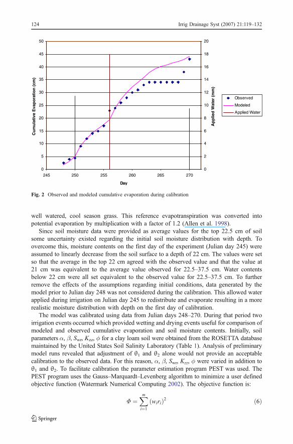
Fig. 2 Observed and modeled cumulative evaporation during calibration
124 Irrig Drainage Syst (2007) 21:119–132
where:
Φ is the objective function to be minimized;m is the number of observations;rI is the residual expressed as the difference between the modeled and observed values;wI is the weight for the ith residual;
The observations used in the calibration were the average moisture contents for the top22.5 cm for Julian days 248–270 and the cumulative evaporation for the same period,which totals 4.3 cm. Weights were applied in Equation 6 to account for differences in themagnitude of observation types. In this case there were measurements of soil water contentwith magnitudes ranging from 0.22 to 0.33 and cumulative evaporation of 4.3 cm. ThePEST manual recommends that weights be calculated as the inverse of the standarddeviation of the observed data. It was assumed that soil water content and cumulativeevaporation measurements had a standard deviation of 0.05 and 0.1 resulting in weights of20 and 10, respectively.
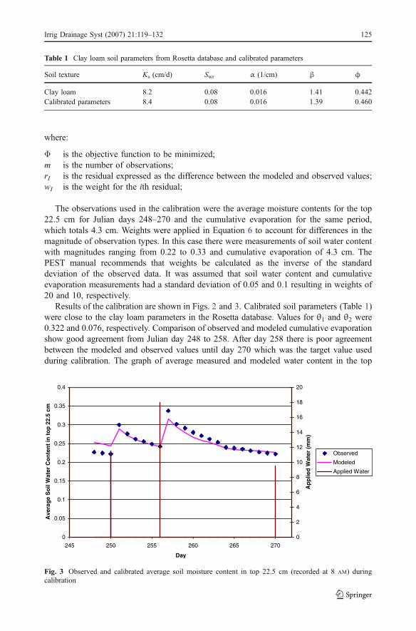
Results of the calibration are shown in Figs. 2 and 3. Calibrated soil parameters (Table 1)were close to the clay loam parameters in the Rosetta database. Values for θ1 and θ2 were0.322 and 0.076, respectively. Comparison of observed and modeled cumulative evaporationshow good agreement from Julian day 248 to 258. After day 258 there is poor agreementbetween the modeled and observed values until day 270 which was the target value usedduring calibration. The graph of average measured and modeled water content in the top
Table 1 Clay loam soil parameters from Rosetta database and calibrated parameters
Soil texture Ks (cm/d) Swr α (1/cm) β φ
Clay loam 8.2 0.08 0.016 1.41 0.442Calibrated parameters 8.4 0.08 0.016 1.39 0.460
0
0.05
0.1
0.15
0.2
0.25
0.3
0.35
0.4
245 250 255 260 265 270
Day
Ave
rag
e S
oil
Wat
er C
on
ten
t in
to
p 2
2.5
cm
0
2
4
6
8
10
12
14
16
18
20
Ap
plie
d W
ater
(m
m)
Observed
Modeled
Applied Water
Fig. 3 Observed and calibrated average soil moisture content in top 22.5 cm (recorded at 8 AM) duringcalibration
Irrig Drainage Syst (2007) 21:119–132 125
22.5 cm show good agreement particularly after the irrigation event on day 250. If bothFigs. 2 and 3 are compared it is interesting to note that the observed evaporation ceasesbetween days 263 and 268 and then increases on days 269 and 270. This is in contrast to thesoil moisture storage which continues to decrease during this period. Because of the anomalyin the observed cumulative evaporation data between days 263 and 270 and the reasonablefit between days 248 to 258, the calibration was considered acceptable. It should also benoted that the moisture content readings from the 5 neutron probe access tubes did differ andit is not clear which values best represent the conditions in the lysimeter.
Model validation
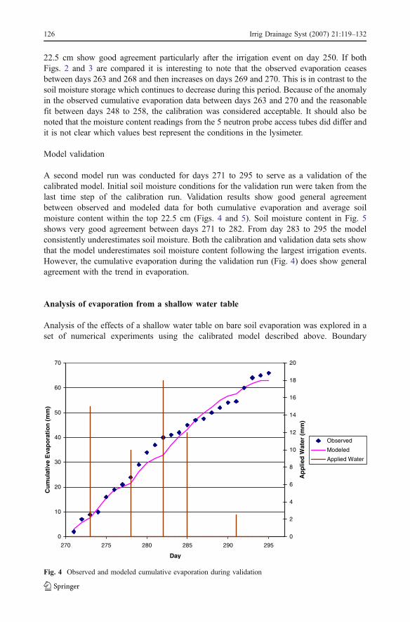
A second model run was conducted for days 271 to 295 to serve as a validation of thecalibrated model. Initial soil moisture conditions for the validation run were taken from thelast time step of the calibration run. Validation results show good general agreementbetween observed and modeled data for both cumulative evaporation and average soilmoisture content within the top 22.5 cm (Figs. 4 and 5). Soil moisture content in Fig. 5shows very good agreement between days 271 to 282. From day 283 to 295 the modelconsistently underestimates soil moisture. Both the calibration and validation data sets showthat the model underestimates soil moisture content following the largest irrigation events.However, the cumulative evaporation during the validation run (Fig. 4) does show generalagreement with the trend in evaporation.
Analysis of evaporation from a shallow water table
Analysis of the effects of a shallow water table on bare soil evaporation was explored in aset of numerical experiments using the calibrated model described above. Boundary
0
10
20
30
40
50
60
70
270 275 280 285 290 295
Day
Cu
mu
lati
ve E
vap
ora
tio
n (
mm
)
0
2
4
6
8
10
12
14
16
18
20
Ap
plie
d W
ater
(m
m)
Observed
Modeled
Applied Water
Fig. 4 Observed and modeled cumulative evaporation during validation
126 Irrig Drainage Syst (2007) 21:119–132
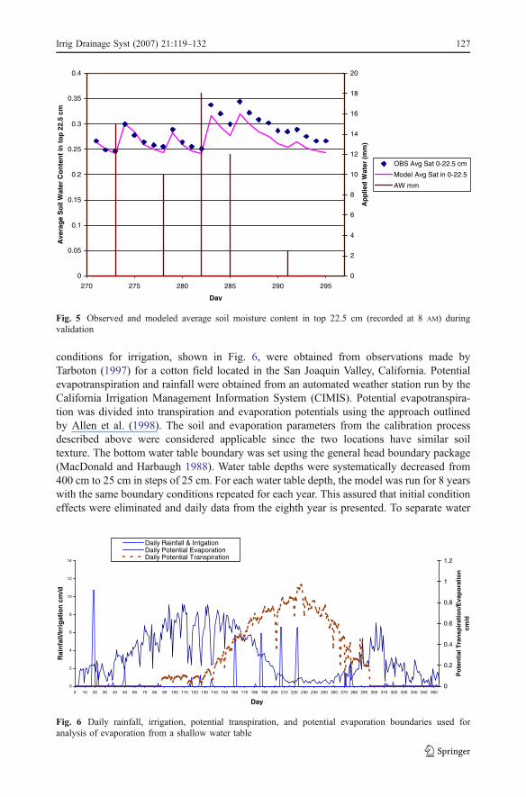
conditions for irrigation, shown in Fig. 6, were obtained from observations made byTarboton (1997) for a cotton field located in the San Joaquin Valley, California. Potentialevapotranspiration and rainfall were obtained from an automated weather station run by theCalifornia Irrigation Management Information System (CIMIS). Potential evapotranspira-tion was divided into transpiration and evaporation potentials using the approach outlinedby Allen et al. (1998). The soil and evaporation parameters from the calibration processdescribed above were considered applicable since the two locations have similar soiltexture. The bottom water table boundary was set using the general head boundary package(MacDonald and Harbaugh 1988). Water table depths were systematically decreased from400 cm to 25 cm in steps of 25 cm. For each water table depth, the model was run for 8 yearswith the same boundary conditions repeated for each year. This assured that initial conditioneffects were eliminated and daily data from the eighth year is presented. To separate water
0
0.05
0.1
0.15
0.2
0.25
0.3
0.35
0.4
270 275 280 285 290 295
Day
Ave
rag
e S
oil
Wat
er C
on
ten
t in
to
p 2
2.5
cm
0
2
4
6
8
10
12
14
16
18
20
Ap
plie
d W
ater
(m
m)
OBS Avg Sat 0-22.5 cm
Model Avg Sat in 0-22.5
AW mm
Fig. 5 Observed and modeled average soil moisture content in top 22.5 cm (recorded at 8 AM) duringvalidation
0
2
4
6
8
10
12
14
0 10 20 30 40 50 60 70 80 90 100 110 120 130 140 150 160 170 180 190 200 210 220 230 240 250 260 270 280 290 300 310 320 330 340 350 360
Day
Rai
nfa
ll/Ir
rig
atio
n c
m/d
0
0.2
0.4
0.6
0.8
1
1.2
Po
ten
tial
Tra
nsp
irat
ion
/Eva
po
rati
on
cm
/d
Daily Rainfall & IrrigationDaily Potential EvaporationDaily Potential Transpiration
Fig. 6 Daily rainfall, irrigation, potential transpiration, and potential evaporation boundaries used foranalysis of evaporation from a shallow water table
Irrig Drainage Syst (2007) 21:119–132 127
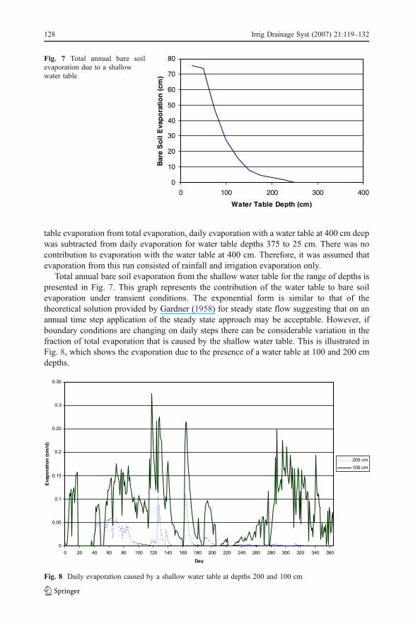
table evaporation from total evaporation, daily evaporation with a water table at 400 cm deepwas subtracted from daily evaporation for water table depths 375 to 25 cm. There was nocontribution to evaporation with the water table at 400 cm. Therefore, it was assumed thatevaporation from this run consisted of rainfall and irrigation evaporation only.
Total annual bare soil evaporation from the shallow water table for the range of depths ispresented in Fig. 7. This graph represents the contribution of the water table to bare soilevaporation under transient conditions. The exponential form is similar to that of thetheoretical solution provided by Gardner (1958) for steady state flow suggesting that on anannual time step application of the steady state approach may be acceptable. However, ifboundary conditions are changing on daily steps there can be considerable variation in thefraction of total evaporation that is caused by the shallow water table. This is illustrated inFig. 8, which shows the evaporation due to the presence of a water table at 100 and 200 cmdepths.
0
10
20
30
40
50
60
70
80
0 100 200 300 400
Water Table Depth (cm)
Bar
e S
oil
Eva
po
rati
on
(cm
)
Fig. 7 Total annual bare soilevaporation due to a shallowwater table
0
0.05
0.1
0.15
0.2
0.25
0.3
0.35
0 20 40 60 80 100 120 140 160 180 200 220 240 260 280 300 320 340 360
Day
Eva
po
rati
on
(cm
/d)
200 cm
100 cm
Fig. 8 Daily evaporation caused by a shallow water table at depths 200 and 100 cm
128 Irrig Drainage Syst (2007) 21:119–132
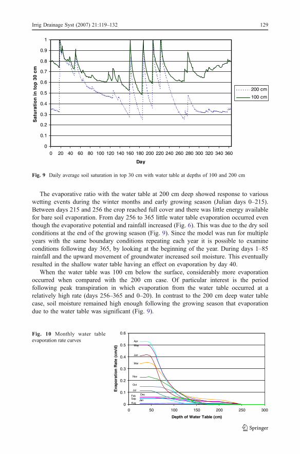
The evaporative ratio with the water table at 200 cm deep showed response to variouswetting events during the winter months and early growing season (Julian days 0–215).Between days 215 and 256 the crop reached full cover and there was little energy availablefor bare soil evaporation. From day 256 to 365 little water table evaporation occurred eventhough the evaporative potential and rainfall increased (Fig. 6). This was due to the dry soilconditions at the end of the growing season (Fig. 9). Since the model was run for multipleyears with the same boundary conditions repeating each year it is possible to examineconditions following day 365, by looking at the beginning of the year. During days 1–85rainfall and the upward movement of groundwater increased soil moisture. This eventuallyresulted in the shallow water table having an effect on evaporation by day 40.
When the water table was 100 cm below the surface, considerably more evaporationoccurred when compared with the 200 cm case. Of particular interest is the periodfollowing peak transpiration in which evaporation from the water table occurred at arelatively high rate (days 256–365 and 0–20). In contrast to the 200 cm deep water tablecase, soil moisture remained high enough following the growing season that evaporationdue to the water table was significant (Fig. 9).
0
0.1
0.2
0.3
0.4
0.5
0.6
0 50 100 150 200 250 300
Depth of Water Table (cm)
Eva
po
rati
on
Rat
e (c
m/d
)
Apr
May
Jun
Mar
Nov
Oct
Jul
DecFeb
JanAug
Sep
Fig. 10 Monthly water tableevaporation rate curves
0
0.1
0.2
0.3
0.4
0.5
0.6
0.7
0.8
0.9
1
0 20 40 60 80 100 120 140 160 180 200 220 240 260 280 300 320 340 360
Day
Sat
ura
tio
n i
n t
op
30
cm
200 cm
100 cm
Fig. 9 Daily average soil saturation in top 30 cm with water table at depths of 100 and 200 cm
Irrig Drainage Syst (2007) 21:119–132 129
MODFLOW evapotranspiration package parameterization
A method for parameterization of the evapotranspiration package in MODFLOW wasdeveloped. Using the results of the model runs with varying water table depths, a set ofcurves relating water table evaporation to water table depth was calculated. These curveswere calculated by averaging the evaporation rate over the period of interest for each watertable depth (monthly curves are shown in Fig. 10). These curves can be used toparameterize the line segments used to define the relationship between water table depthand evapotranspiration rate in MODFLOW 2000.
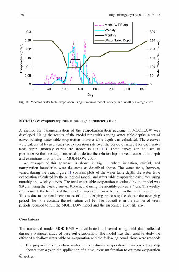
An example of this approach is shown in Fig. 11 where irrigation, rainfall, andtranspiration boundaries were the same as described above. The water table, however,varied during the year. Figure 11 contains plots of the water table depth, the water tableevaporation calculated by the numerical model, and water table evaporation calculated usingmonthly and weekly curves. The total water table evaporation calculated by the model was8.9 cm, using the weekly curves, 9.5 cm, and using the monthly curves, 9.4 cm. The weeklycurves match the features of the model’s evaporation curve better than the monthly example.This is due to the non-linear nature of the underlying processes; the shorter the averagingperiod, the more accurate the estimation will be. The tradeoff is in the number of stressperiods required to run the MODFLOW model and the associated input file size.
Conclusions
The numerical model MOD-HMS was calibrated and tested using field data collectedduring a lysimeter study of bare soil evaporation. The model was then used to study theeffect of a shallow water table on evaporation and the following conclusions were reached:
1. If a purpose of a modeling analysis is to estimate evaporative fluxes on a time stepshorter than a year, the application of a time invariant function to estimate evaporation
0
0.05
0.1
0.15
0.2
0.25
0.3
0 50 100 150 200 250 300 350
Day
Eva
po
rati
on
(cm
/d)
0
50
100
150
200
250
300
Wat
er T
able
Dep
th (
cm)
Model WT Evap
Weekly
Monthly
Water Table Depth
Fig. 11 Modeled water table evaporation using numerical model, weekly, and monthly average curves
130 Irrig Drainage Syst (2007) 21:119–132
from a water table in an irrigated setting is not recommended due to the transient natureof soil moisture.
2. In arid irrigated regions where the soil is dry after crop harvest, little or no evaporationfrom a shallow water table will occur until the soil profile has been rewetted by rainfall,irrigation, or upward water movement from the water table.
3. The MODFLOW evapotranspiration package can be parameterized to estimate theshallow water table portion of total evapotranspiration using the results of a 1-Dvariably saturated flow model analysis based on an irrigation, rainfall, and transpirationregime typical to the model study area. Due to the non-linearity of the underlyingprocesses, the shorter the time period used in creating the average evaporation curvesthe more accurate the estimation of evaporation.
Acknowledgements We would like to acknowledge the suuport of the USDA Fund For Rural America, theUSBR Fresno office, and the UC Salinity Drainage Program.
References
Allen, RG, Pereira LS, Raes D, Smith M (1998) Crop evapotranspiration – guidelines for computing cropwater requirements – FAO irrigation and drainage paper 56. FAO – Food and Agricultural Organizationof the United Nations, Rome
Banta ER (2000) Modflow 2000, the U.S. Geological Survey modular ground-water model – documentationof packages for simulating evapotranspiration with a segmented function (ETS1) and drains with returnflow (DRT1). Open File Report 00-466. U.S. Geological Survey, Washington, DC, p 127
Belitz K, Phillips SP, Gronberg JM (1993) Numerical simulation of ground-water flow in the central part ofthe Western San Joaquin Valley, California. U.S. Geological Survey Water-Supply Paper 2396.Sacramento, Ca., p 69
Eching SO, Hopmans JW, Wallender WW, MacIntyre JL, Peters D (1994) Estimation of local and regionalcomponents of drain-flow from an irrigated field. Irrig Sci 15:153–157
Gardner WR (1958) Some steady-state solutions of the unsaturated moisture flow equation with applicationto evaporation from a water table. Soil Sci 85:228–232
Gardner WR, Fireman M (1958) Laboratory studies of evaporation from soil columns in the presence of awater table. Soil Sci 85:244–249
Jorenush MH, Sepaskhah AR (2003) Modelling capillary rise and soil salinity for shallow saline water tableunder irrigated and non-irrigated conditions. Agric Water Manag 61:125–141
Katul GG, Parlange MB (1992) A Penman–Brutsaert model for wet surface evaporation. Water Resour Res28:121–126
McDonald MG, Harbaugh AH (1988) A modular three-dimensional finite-difference ground-water flowmodel. In: Techniques of water resources investigations of the United States geological survey, Book 6,chap. A1, U.S. Geol. Surv., Washington, DC.
Panday S, Huyakorn PS (2004) A fully coupled physically-based spatially-distributed model for evaluatingsurface/subsurface flow. Adv Water Resour 27:361–382
Parlange MB, Katul GG, Cuenca RH, Kavvas ML, Nielsen DR, Mata M (1992) Physical basis for a timeseries model of soil water content. Water Resour Res 28:2437–2446
Parlange MB, Katul GG, Folegatti MV, Nielsen DR (1993) Evaporation and the field scale soil waterdiffusivity function. Water Resour Res 29:1279–1286
Prathapar SA, Robbins CW, Meyer WS, Jayawardane NS (1992) Models for estimating capillary rise in aheavy clay soil with a saline shallow water table. Irrig Sci 13:1–7
Ritchie JT (1972) Model for predicting evaporation from a row crop with incomplete cover. Water ResourRes 8:1204–1213
San Joaquin Valley Drainage Program (1990) A management plan for agricultural subsurface drainage andrelated problems on the westside San Joaquin Valley. San Joaquin Valley Drainage Program,Sacramento, CA, p 183
Saravanapavan T, Saluvucci GD (2000) Analysis of rate-limiting processes in soil evaporation withimplications for soil resistance models. Adv Water Resour 23:493–502
Irrig Drainage Syst (2007) 21:119–132 131

Šimůnek J, Šejna M, van Genuchten MTh (1998) The HYDRUS-1D software package for simulating theone-dimensional movement of water, heat, and multiple solutes in variably-saturated media, Version 2.0,IGWMC- TPS-70. International Ground Water Modeling Center, Colorado School of Mines, Golden,Colorado, pp 202
Soppe RWO, Ayars JE (2003) Characterizing ground water use by safflower using weighing lysimeters.Agric Water Manag 60(1):59–71
Tarboton KC (1997) Integrated hydrological model for irrigation drainage management. DoctoralDissertation, University of California, Davis. Davis, CA, p 362
Wallender WW, Grimes DW, Henderson DW, Stromberg LK (1979) Estimating the contribution of a perchedwater table to the seasonal evapotranspiration of cotton. Agron J 71:1056–1060
Watermark Numerical Computing (2002) PEST – Model independent parameter estimation. WatermarkNumerical Computing, p 279
Yang J, Li B, Liu S (2000) A large weighing lysimeter for evapotranspiration and soil–water–groundwaterexchange studies. Hydrol Process 2000:1887–1897
132 Irrig Drainage Syst (2007) 21:119–132


