Vol.1, No.1, 1-9 (2010) doi:10.4236/as.2010.11001

Copyright © 2010 SciRes. Openly accessible at http://www.scirp.org/journal/as/

Agricultural Sciences

Modification of water application uniformity among closed circuit trickle irrigation systems

Hani A.-G. Mansour1*, Mohamed Yousif Tayel1, Mohamed A. Abd El-Hady1, David A. Lightfoot2, Abdel-Ghany Mohamed El-Gindy3

1Water Relations and Field Irrigation Department, National Research Centre, Giza, Egypt; *Corresponding Author: hanimansour88@yahoo.com 2Soil & Plant and Agricultural Systems Department, Southern Illinois University, Carbondale, USA 3Agricultural Engineering Department, Faculty of Agriculture, Ain Shams University, Cairo, Egypt

Received 2 April 2010; revised 30 April 2010; accepted 5 May 2010.

ABSTRACT

The aim of this research was determine the ma- ximum application uniformity of closed circuit trickle irrigation systems designs. Laboratory tests carried out for Two types of closed circuits: a) One manifold for lateral lines or Closed cir-cuits with One Manifold of Trikle Irrigation Sys-tem (COMTIS); b) Closed circuits with Two Manifolds of Trikle Irrigation System (CTMTIS), and c) Traditional Trikle Irrigation System (TTIS) as a control. Three lengths of lateral lines were used, 40, 60, and 80 meters. PE tubes lateral lines: 16 mm diameter; 30 cm emitters distance, and GR built-in emitters 4 lph when operating pressure 1 bar. Experiments were conducted at the Agric. Eng. Res. Inst., ARC, MALR, Egypt. With COMTIS the emitter flow rate was 4.07, 3.51, and 3.59 lph compared to 4.18, 3.72, and 3.71 lph with CTMTIS and 3.21, 2.6, and 2.16 lph with TTIS (lateral lengths 40, 60, and 80 meters respec-tively). Uniformity varied widely within individual lateral lengths and between circuit types. Under CTMTIS uniformity values were 97.74, 95.14, and 92.03 %; with COMTIS they were 95.73, 89.45, and 83.25 %; and with TTIS they were 88.27, 84.73, and 80.53 % (for lateral lengths 40, 60, 80 meters respectively). The greatest uniformity was observed under CTMTIS and COMTIS when using the shortest lateral length 40 meters, then lateral length 60 meters, while the lowest value was observed when using lateral length 80 me-ters this result depends on the physical and hy-draulic characteristics of the emitter and lateral line. CTMTIS was more uniform than either COMTIS or TTIS. Friction losses were decreased with CTMTIS in the emitter laterals at lengths 40 meters compared to TTIS and COMTIS. There-fore, differences may be related to increased

friction losses when using TDIS and COMDIS.

Keywords: Trickle Irrigation; Closed Circuits; Manifold; Lateral; Flow Rate; Uniformity

1. INTRODUCTION

Trickle irrigation has been used since ancient times when buried clay pots were filled with water, which would gradually seep into the grass. Perforated pipe was intro-duced in Germany in the 1920s and in 1934, Nobey ex-perimented with irrigating through porous canvas hose at Michigan State University. Plastic microtubing and vari-ous types of emitters began to be used in the greenhouses of Europe and the United States.

Qualitative classification standards for the production of emitters, the emitter discharge rate q (m3/h) has been described by a power law, = xq kH , where operating pressure head H (m), emitter coefficient (k), and expo-nent (x) depend on emitter characteristics [1]. Capra and Scicolone [2] indicated that the major sources of emitter flow rate variations are emitter design, the material used to manufacture the lateral line, and precision. According to [3] the main factors affecting trickle irrigation system uniformity are: 1) manufacturing variations in emitters and pressure regulators, 2) pressure variations caused by elevation changes, 3) friction head losses throughout the pipe network, 4) emitter sensitivity to pressure and irriga-tion water temperature changes, and 5) emitter clogging. Similarly, according to the manufacturer’s coefficient of emitter variation (CVm), have been developed by ASAE. CVm values below 10% are suitable and > 20% are un-acceptable [4]. The emitter discharge variation rate (qvar) should be evaluated as a design criterion in trickle irriga-tion systems; qvar < 10% may be regarded as good and qvar > 20% as unacceptable [5,6]. The acceptability of micro-irrigation systems has also been classified accord-

H. A.-G. Mansour et al. / Agricultural Sciences 1 (2010) 1-9

Copyright © 2010 SciRes. Openly accessible at http://www.scirp.org/journal/as/

2

ing to the statistical parameters, Uqs and EU; namely, EU = 94%-100% and Uqs = 95%-100% are excellent, and EU < 50% and Uqs < 60% are unacceptable [7]. Ortega et al [8] calculated emission uniformity (EU), pressure variation coefficient (VCp), and flow variation coeffi-cient per emitter (VCq) at localized systems and reported that they were 84.3%, 0.12, and 0.19, respectively. They classified the systems unacceptable for VCq > 0.4 and excellent for VCq < 0.1. In addition to pressure variation along irrigation tape, variation in emitter structure or emitter geometry has been known to cause poor uniform-ity of emitter discharge [1,5,9]. Differences in emitter geometry may be caused by variation in injection pres-sure and heat instability during their manufacture, as well as by a heterogeneous mixture of materials used for the production [1]. Berkowitz [10] observed reductions in emitter irrigation flow ranging from 7 to 23% at five sites observed. Reductions in scouring velocities were also observed from the designed 0.6 m/s (2ft/s) to 0.3 m/s (1ft/s). Lines also developed some slime build-up, as reflected by the reduction in scouring velocities, but this occurred to a less degree with higher quality effluent. In their treatments they generally used approximate friction equations such as Hazen-Williams and Scobey, neglected the variation of the velocity head along the lateral and assumed initial uniform emitter flow. Warrick & Yitayew [11] assumed a lateral with a longitudinal slot and pre-sented design charts based on spatially varied flow. The latter solution has neglected the presence of laminar flow in a considerable length of the downstream part of the lateral. Hathoot et al [12] provided a solution based on uniform emitter discharge but took into account the change of velocity head and the variation of Reynold’s number. They used the Darcy-Weisbach friction equation in estimating friction losses. Hathoot et al [13] consid-ered individual emitters with variable outflow and pre-sented a step by step computer program for designing either the diameter or the lateral length. In this study we considered the pressure head losses due to emitters pro-trusion. These losses occur when the emitter barb protru-sion obstructs the water flow. Three sizes of emitter barbs were specified, small, medium and large in which the small barb has an area equal or less than 20 mm², the medium barb has an area between 21-31mm² and the large one has an area equal to or more than 32 mm². The objectives of the present research were:

1) Recovery the problem of pressure reduction at the end stage of lateral lines.

2) Investigate emitter discharge application uniformity and its dependence on operation pressures and Laterals lengths (40, 60, and 80 m).

3) To compare emitter discharge uniformity between tow type of closed circuits (COMTIS and CTMTIS) and traditional trickle system (TTIS).

2. MATIRIALS AND METHODS 2.1. Site Location and Experimental Design

This experiment was conducted at Irrigation Devices and Equipments Tests Laboratory, Agricultural Engineering Research Institute, Agriculture Research Center, Cairo, Egypt. The experimental design was randomized com-plete block with three replicates. Three irrigation new lateral lines 40, 60, 80 m long that were installed at con-stant level and under ten operating pressures 0.2, 0.4, 0.6, 0.8, 1.0, 1.2, 1.4, 1.6, 1.8, and 2.0 bar for ten minutes at each pressure. Details of the pressure and water supply control have been described by [14], to evaluate the Built-in Dripper (GR), discharge, 4 lph design emitter spacing of 30 cm at 1 bar nominal operating pressure in order to reach an modified way to resolve the problem of lack of pressure at the end of lateral lines in the tradi-tional trickle irrigation system.

2.2. Trickle Irrigation Components

The components of closed circuits the trickle system include, supply lines, control valves, supply and return manifolds, trickle lateral lines, trickle emitters, check valves and air relief valves/vacuum breakers. Figures 1 and 2 show the closed circuits of trickle irrigation sys-tem: 1) Closed circuit with Tow Manifold of trickle Irri-gation System (CTMTIS) and 2) Closed circuit with One Manifold of trickle Irrigation System (COMTIS) while Figure 3 is 3) Traditional of Trickle Irrigation System (TTIS). Supply lines provide water to the supply mani-folds of the system after passing through the zone con-trol valve in systems with more than one zone. The sup-ply manifold distributes water to the individual trickle laterals within the zone. The laterals then connect to a return manifold. Along the supply and return manifold, air relief/vacuum breakers are installed at the highest point of the manifolds to allow air to enter the system during depressurization [15]. The return manifold is used during system flushing to collect water from the laterals and carry it to the return line which returns to the pre-treatment device. Prior to connecting the return manifold to the return line a check valve is installed to prevent water from entering the zone during the operation of other zones.

max minvar

max

q qq

q

(1)

SCV

q (2)

1

1

n

ni

qi qUC

q

(3)

where:

H. A.-G. Mansour et al. / Agricultural Sciences 1 (2010) 1-9

Copyright © 2010 SciRes. Openly accessible at http://www.scirp.org/journal/as/

3

Figure 1. Layout of Closed circuit with Tow Manifolds of Trickle Irrigation System (CTMTIS).

Figure 2. Layout of Closed circuits with One Manifold of Trickle Irrigation System (COMTIS).

Figure 3. Layout of Traditional Trickle Irrigation System (TTIS).

qmax and qmin are maximum and minimum emitter

discharge, respectively, q and S are the mean and

standard deviation, respectively, of discharge (q), and n is the number of emitters.

Emission uniformity of the quarter was calculated us-ing the equation [8]

25 100%qqEU (4)

where: 25q % is the mean of the lowest 0.25 of emitter dis-

charge. The coefficient of variation in this calculation refers to

the depth of water applied. This statistical uniformity coefficient describes the uniformity of water distribution assuming a normal distribution of flow rates from the emitters.

H. A.-G. Mansour et al. / Agricultural Sciences 1 (2010) 1-9

Copyright © 2010 SciRes. Openly accessible at http://www.scirp.org/journal/as/

4

Application uniformity of a system is affected by hy-draulic design, topography, operating pressure, pipe size, emitter spacing, and emitter discharge variability. Dis-charge variability is due to manufacturer’s coefficient of variation, emitter wear, and emitter plugging [7]. Table 1 illustrates the acceptability depending on the range of statistical uniformity. ASAE [16] also represents flow variation through the Christiansen Uniformity Coeffi-cient:

1 qu q

C (5)

where: Cu = the uniformity coefficient %,

q = the mean emitter flow (lph), and

q = the mean absolute deviation from the mean

emitter flow (lph). An additional method of evaluating the application

uniformity of a system is described in [17]. This method uses a distribution uniformity using the average depth of application of the lower quartile over the average depth of application (Equation (8)). This method has been used by USDA and NRCS since the 1940s.

avg .low quarter depthavg .depth of water accumulated in aallelmentsDUlq

(6)

2.2.1. Head Loss in a Pipe The head loss in pipes due to water flow is proportional to the pipe’s length.

HJ

L

(7)

where J = The head loss in a pipe is usually expressed by either %.

The head loss due to friction is calculated by Hazen- Williams equation [18]:

12 1 852 4 871 21 10 ( ) . .QJ . x D

C

(8)

where: J = head loss is expressed by (m/100 m) or %. Q = flow rate is expressed by m³/h. D = Inside diameter of a pipe is expressed by mm. C = (Hazen-Williams coefficient) smoothness (the

roughness) of the internal pipe, (the range for a commer-cial pipe is 100 – 150)

For polyethelene tubes when diameter < 40 mm and (C = 150) [19,20].

For laminar flow [21] where R 2000 the coefficient

Table 1. Methods of comparison of statistical uniformity [7].

Method Ac-ceptability

Statistical Uniformity, Us (%)

Excellent 95-100 Good 85-90 Fair 75-80 Poor 65-70

Unacceptable <60

of friction is given by: 64

fR

(9)

in which R, Reynolds number is given by: VD

R

(10)

where: R = Reynolds number,

V = flow velocity (m/s), D = inside diameter (m), and ν = kinematic viscosity of irrigation water. Critical velocity could be calculated by (10) and the

following equations. For turbulent flow (3000 R 105) the Blasius

equation can be used: 25.0R316.0f (11)

For fully turbulent flow, 105 R 107, Watters and Keller [22] recommended the following equation:

172.0R13.0f (12)

2.3. Statistical Analysis

All the collected data were subjected to the statistical analysis as the usual technique of analysis of variance (ANOVA) and the least significant difference (L.S.D) between systems at 5% had been done according to [23]. 3. RESULTS AND DISCUSSION

3.1. The Effect of Closed Circuits at Different Laterals Lengths on Emitter Discharge and the Cumulative Flow Lines Subsidiary

1) Closed circuits with tow manifolds of trickle irriga-tion system (CTMDIS):

Data of Figures 4(a), 4(b) and 4(c) indicate the effect of closed circuits with tow manifolds of trickle irrigation system (CTMTIS) at different laterals lengths (40, 60, and 80 m) on dripper flows and the Cumulative flows lines subsidiary. Under the lateral lines length (40 m), emitter flow was the highest value (4.18 lph), then came the lateral line length (60 m) value was 3.72 lph. The lowest value was 3.71 lph achieved under lateral line length (80 m). While as for the cumulative flow under lateral length (80 m) was the highest (990.0 lph), then lateral length (60 m) (744.0 lph), while the lowest value of the cumulative flow was 599.9 under lateral length (40 m) as shown in Figures 4(a), 4(b) and 4(c) at (1.0 bar) operating pressure and under the laboratory condi-tions as stated by [14,22,24,25]. There were significant differences at the 5% level in the emitters flow and the cumulative flows between any two lateral lengths of CTMTIS. The increase in emitters flow and the cumulative

H. A.-G. Mansour et al. / Agricultural Sciences 1 (2010) 1-9

Copyright © 2010 SciRes. Openly accessible at http://www.scirp.org/journal/as/

5

Cu

mu

lati

ve

Flo

w (

Lp

h)

0

1

2

3

4

5

0 5 10 15 20 25 30 35 40

0

200

400

600

800

1000

1200

Dripper flow(L/h) Cumulative(L/h)

0

1

2

3

4

5

0 5 10 15 20 25 30 35 40 45 50 55 60

0

200

400

600

800

1000

1200

Dripper flow(L/h) Cumulative(L/h)

(b)

0

1

2

3

4

5

0 5 10 15 20 25 30 35 40 45 50 55 60 65 70 75 80

0

200

400

600

800

1000

1200

Dripper flow(L/h) Cumulative(L/h)

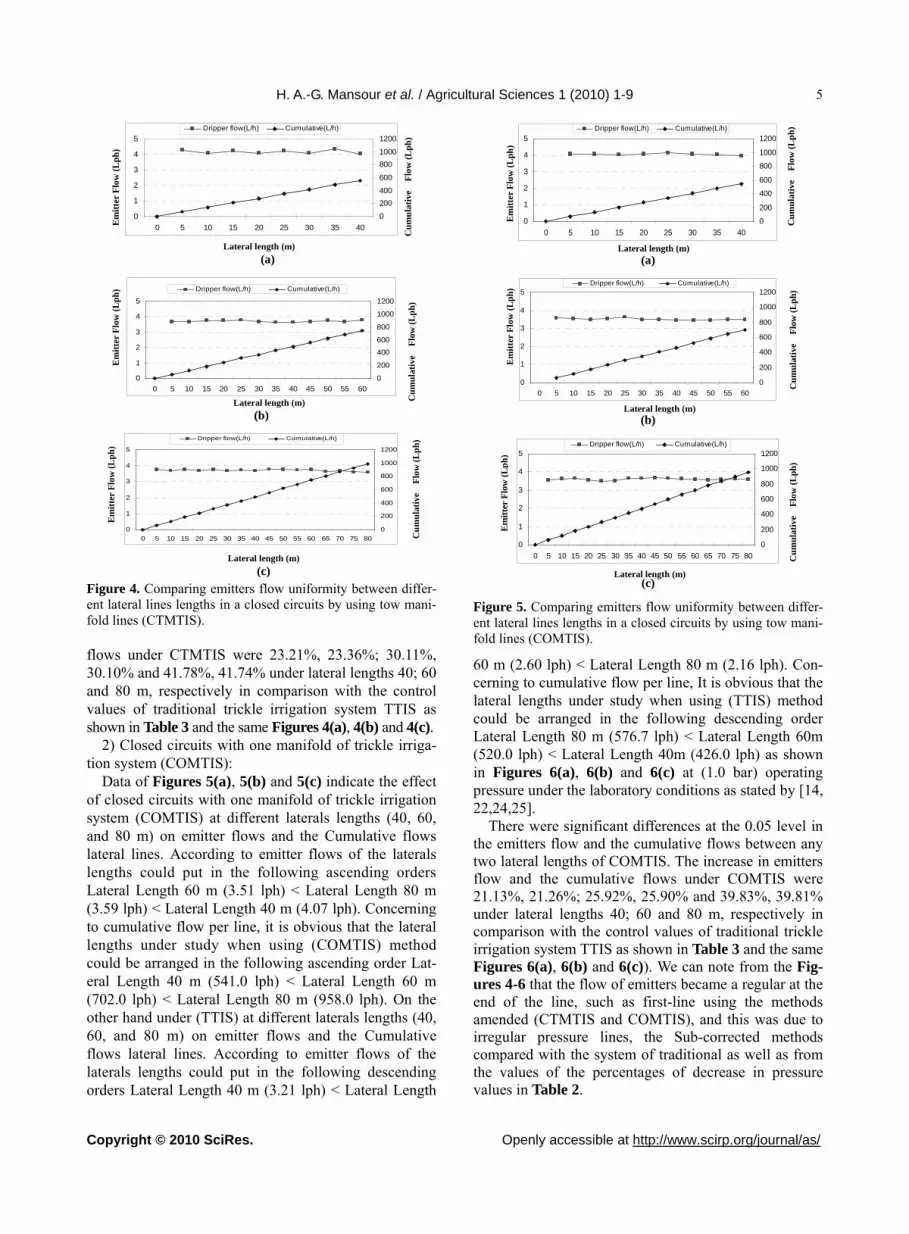
Figure 4. Comparing emitters flow uniformity between differ-ent lateral lines lengths in a closed circuits by using tow mani-fold lines (CTMTIS). flows under CTMTIS were 23.21%, 23.36%; 30.11%, 30.10% and 41.78%, 41.74% under lateral lengths 40; 60 and 80 m, respectively in comparison with the control values of traditional trickle irrigation system TTIS as shown in Table 3 and the same Figures 4(a), 4(b) and 4(c).

2) Closed circuits with one manifold of trickle irriga-tion system (COMTIS):

Data of Figures 5(a), 5(b) and 5(c) indicate the effect of closed circuits with one manifold of trickle irrigation system (COMTIS) at different laterals lengths (40, 60, and 80 m) on emitter flows and the Cumulative flows lateral lines. According to emitter flows of the laterals lengths could put in the following ascending orders Lateral Length 60 m (3.51 lph) < Lateral Length 80 m (3.59 lph) < Lateral Length 40 m (4.07 lph). Concerning to cumulative flow per line, it is obvious that the lateral lengths under study when using (COMTIS) method could be arranged in the following ascending order Lat-eral Length 40 m (541.0 lph) < Lateral Length 60 m (702.0 lph) < Lateral Length 80 m (958.0 lph). On the other hand under (TTIS) at different laterals lengths (40, 60, and 80 m) on emitter flows and the Cumulative flows lateral lines. According to emitter flows of the laterals lengths could put in the following descending orders Lateral Length 40 m (3.21 lph) < Lateral Length

0

1

2

3

4

5

0 5 10 15 20 25 30 35 40

0

200

400

600

800

1000

1200Dripper flow(L/h) Cumulative(L/h)

Cu

mu

lati

ve

Flo

w (

Lp

h)

Em

itte

r F

low

(L

ph

)

Em

itte

r F

low

(L

ph

)

Lateral length (m)

(a) (a) Lateral length (m)

0

1

2

3

4

5

0 5 10 15 20 25 30 35 40 45 50 55 60

0

200

400

600

800

1000

1200Dripper flow(L/h) Cumulative(L/h)

Em

itte

r F

low

(L

ph

)

Cu

mu

lati

ve

Flo

w (

Lp

h)

Em

itte

r F

low

(L

ph

)

Cu

mu

lati

ve

Flo

w (

Lp

h)

Lateral length (m)

(b) Lateral length (m)

Cu

mu

lati

ve

Flo

w (

Lp

h)

0

1

2

3

4

5

0 5 10 15 20 25 30 35 40 45 50 55 60 65 70 75 80

0

200

400

600

800

1000

1200Dripper flow(L/h) Cumulative(L/h)

Em

itte

r F

low

(L

ph

)

Em

itte

r F

low

(L

ph

)

Cu

mu

lati

ve

Flo

w (

Lp

h)

Lateral length (m)

(c) (c)

Lateral length (m)

Figure 5. Comparing emitters flow uniformity between differ-ent lateral lines lengths in a closed circuits by using tow mani-fold lines (COMTIS).

60 m (2.60 lph) < Lateral Length 80 m (2.16 lph). Con-cerning to cumulative flow per line, It is obvious that the lateral lengths under study when using (TTIS) method could be arranged in the following descending order Lateral Length 80 m (576.7 lph) < Lateral Length 60m (520.0 lph) < Lateral Length 40m (426.0 lph) as shown in Figures 6(a), 6(b) and 6(c) at (1.0 bar) operating pressure under the laboratory conditions as stated by [14, 22,24,25].

There were significant differences at the 0.05 level in the emitters flow and the cumulative flows between any two lateral lengths of COMTIS. The increase in emitters flow and the cumulative flows under COMTIS were 21.13%, 21.26%; 25.92%, 25.90% and 39.83%, 39.81% under lateral lengths 40; 60 and 80 m, respectively in comparison with the control values of traditional trickle irrigation system TTIS as shown in Table 3 and the same Figures 6(a), 6(b) and 6(c)). We can note from the Fig-ures 4-6 that the flow of emitters became a regular at the end of the line, such as first-line using the methods amended (CTMTIS and COMTIS), and this was due to irregular pressure lines, the Sub-corrected methods compared with the system of traditional as well as from the values of the percentages of decrease in pressure values in Table 2.

H. A.-G. Mansour et al. / Agricultural Sciences 1 (2010) 1-9

Copyright © 2010 SciRes. Openly accessible at http://www.scirp.org/journal/as/

6

3) Uniformity coefficient under different lateral lengths of closed circuits methods:

0

1

2

3

4

5

0 5 10 15 20 25 30 35 40

Dripper flow(L/h) line flow

0

200

400

600

800

1000

1200

Em

itte

r F

low

(L

ph

) E

mit

ter

Flo

w (

Lp

h)

Em

itte

r F

low

(L

ph

)

Uniformity coefficient under CTMTIS were the high-est values (97.74%; 95.14% and 92.03%), then COMTIS (95.73%; 89.45% and 83.25%), while the lowest values of uniformity coefficient was 88.27%; 84.73% and 80.53% under TTIS when using three laterals line lengths (40, 60 and 80 m), respectively as stated by [4], as shown in Table 3. That LSD 0.05 value was (2.5) and (2.1) show there are significant differences in uniformity coefficient between all lateral lengths in each connection methods of irrigation, with the exception of that between CTMTIS and COMTIS in the same lateral lengths 40m. The increases percentage in uniformity coefficient under CTMTIS were 9.68%; 10.94% and 12.49 %, while the increases percentage under COMTIS were 7.79%; 5.27% and 3.26% at three lateral lengths 40, 60, and 80 m, re-spectively relative to TTIS. According to the uniformity coefficient, the interaction between the connection methods and lateral lengths treatments was significant, as stated [5,6,8,26] about the classification of acceptabil-ity of trickle irrigation system.

Lateral length (m)

(a)

0

1

2

3

4

5

0 5 10 15 20 25 30 35 40 45 50 55 60

0

200

400

600

800

1000

1200Dripper flow(L/h) Cumulative(L/h)

Cu

mu

lati

ve

Flo

w (

Lp

h)

(b) Lateral length (m)

0

1

2

3

4

5

0 5 10 15 20 25 30 35 40 45 50 55 60 65 70 75 80

0

200

400

600

800

1000

1200Dripper flow(L/h) Cumulative(L/h)

Cu

mu

lati

ve

Flo

w (

Lp

h)

The variation is in uniformity coefficient between the lateral lengths under CTMTIS and COMTIS according to LSD at 0.05 values and Figure 7. Due to hydraulics, and adjusted friction loss in lateral lines values for new irrigation methods are shown in Figure 8.

Lateral length (m)

(c)

4) Effect of closed circuits methods and lateral length on friction loss:

Figure 6. Comparing emitters flow uniformity between differ-ent lateral lines lengths under trickle traditional system (TTIS).

Table 2. Effect of the closed circuits irrigation methods on emitter flow and cumulative flow.

Irrigation Method Lateral Length

(m)

Emitter Flow (lph)

Reduction Pres-sure (%)

Cumulative Flow (lph)

40 4.18 3.70 555.9 60 3.72 5.60 744.0 CTMTIS 80 3.71 7.00 990.0 40 4.07 3.99 541.0 60 3.51 6.10 702.0 COMTIS 80 3.59 8.90 958.0 40 3.21 8.35 426.0 60 2.60 13.87 520.0 TTIS 80 2.16 30.58 576.7

LSD 0.05 0.03 0.24 3.3

Table 3. Effect of closed methods and lateral lengths on uniformity coefficient (%) and friction loss (bar).

Irrigation con-nection Method

Lateral Length

(m)

Uniformity Coefficient,%

Coefficient Variation (CV)

Acceptability By ASAE 1996

Friction Loss

(bar) 40 97.74 0.08 Excellent 0.050 60 95.14 0.06 Excellent 0.130 CTMTIS 80 92.03 0.12 good 0.170 40 95.73 0.07 Excellent 0.080

60 89.45 0.16 good 0.170 COMTIS 80 83.25 0.23 good 0.250

40 88.27 0.18 good 0.114

60 84.73 0.22 good 0.221 TTIS 80 80.53 0.28 fair 0.400

LSD 0.05 0.21 0.01

H. A.-G. Mansour et al. / Agricultural Sciences 1 (2010) 1-9

Copyright © 2010 SciRes. Openly accessible at http://www.scirp.org/journal/as/

7

Figure 7. Effect of lateral length on uniformity coefficient under closed circuit with one or two manifolds of trickle irrigation system (COMTIS) or (CTMTIS).

Figure 8. Effect of lateral length on friction loss under closed circuits with one or two manifolds of trickle irrigation system (COMTIS) or (CTMTIS).

According to friction loss as shown in Figure 8, the

lowest values (0.05; 0.13 and 0.17 bar) were under CTMTIS, then COMTIS values of friction loss were 0.08; 0.17 and 0.25 bar, while the highest values were under TTIS (0.114; 0.221 and 0.4 bar) when using three lateral lines lengths (40; 60 and 80 m), respectively as stated by [11-13]. The variation in uniformity coefficient between the lateral lengths under CTMTIS and COMTIS according to LSD at 0.05 values and Figures 3 and 4. Due to hydraulics, and adjusted friction loss in lateral lines values for new irrigation methods are shown in Figure 8.

As shown LSD 0.05 values in Table 4 there are sig-nificant differences in friction loss values between all lateral lengths and all methods. The decrease percentage in friction loss under CTMTIS were 56.14%; 41.17% and 57.50%, while the decrease percentage under COMTIS were 29.82; 23.07 and 37.50 at three lateral lengths (40; 60 and 80), respectively. According to the friction losses, The interaction between the connection methods and lat-eral lengths treatments was significant and the main rea-son of increase uniformity coefficient of closed circuits methods CTMTIS and COMTIS is that the friction loss decreased significantly under these methods Data as we can note the data in Tables 3 and 4.

The study is confirms that the closed circuits of trickle irrigation systems (CTMTIS) and (COMTIS) by some modifications in manifolds and laterals are; generally, polyethylene pipes of (0% slope) fixed level and fitted with similar and equally spaced emitters whose dis-charges usually decrease in the head losses along the lines with flow direction which led to that increase in the above-described Uniformity coefficients as shown in Tables 3 and 4 and Figures 7 and 8. Many investigators provided approximate solutions for the problem of trickle irrigation lateral design. Among the earlier inves-tigators were [14,22,24,25].

5) Effect of different operating pressures on emitters discharge of lateral lines closed circuits:

In Table 5 we can be observed there was a direct rela-tionship between the operating pressures and the average discharge of lateral lines along the lines in all cases and this is logical. When operating pressure 0.8 bar was un-der used CTMTIS method, the average of emitter dis-charge when lateral length 40 m was 4.48 lph and when using the COMTIS and the value of the average dis-charge of emitter was 4.20 lph under the same length of the line.

While with the change in the operating pressure it’s increased to 1.0 bar. When the length of lateral lines was

H. A.-G. Mansour et al. / Agricultural Sciences 1 (2010) 1-9

Copyright © 2010 SciRes. Openly accessible at http://www.scirp.org/journal/as/

8

Table 4. Effect of operating pressures 1.0 bar on the flow parameters of PE lateral tubes.

LL (m) of TTIS

LL (m) of CTMTIS

LL (m) of COMTIS Hydraulic

Parameters 40 60 80 40 60 80 40 60 80

No. of emitters

133 200 267 133 200 267 133 200 267

Emitter (Q) (lph) 3.21 2.60 2.16 4.18 3.72 3.71 4.07 3.51 3.59

Total (Q) (lph) 427 520 577 556 744 990 541 702 958

Velocity avg. m/s 0.94 1.62 1.97 0.86 1.54 1.88 0.91 1.73 1.92

Renold Number 3234 3489 3612 3238 3001 3062 3859 3753 3810

Flow Type Turbulent

Critical Velocity 0.89 1.58 1.93 0.82 1.48 2.83 0.87 1.68 1.85

f = ε /d 0.23

Hf (bar) 0.114 0.221 0.400 0.050 0.130 0.170 0.080 0.170 0.250

ε /d = Roughens Coefficient; LL = Lateral Length (m); Rn > 3000 = Turblent flow; Rn < 3000 = Laminar flow.

Table 5. Effect of operating pressures (bar) on discharges of the closed circuits.

Discharge values (lph)

Lateral lengths(m) of TTIS

Lateral lengths(m) of CTMTIS

Lateral lengths(m) of COMTIS

Pressure

(bar)

40 60 80 40 60 80 40 60 80

0.2 1.35 1.26 0.89 2.00 2.15 2.30 1.66 1.48 1.11

0.4 1.50 1.39 1.01 2.60 2.35 2.63 2.00 1.84 1.53

0.6 1.84 1.58 1.15 3.87 3.35 3.67 2.88 2.31 2.25

0.8 2.25 1.82 1.37 4.38 3.74 3.74 4.20 3.40 3.37

1.0 2.93 2.18 1.73 4.48 3.94 3.86 4.33 3.57 3.68

1.2 3.10 2.49 1.98 4.52 4.02 3.94 4.41 3.69 3.71

1.4 3.24 2.98 2.23 4.59 4.11 4.15 4.53 3.78 3.80

1.6 3.47 3.35 2.52 4.64 4.27 4.31 4.64 3.96 3.92

1.8 3.65 3.49 2.88 4.70 4.33 4.43 4.70 4.15 4.13

2.0 3.84 3.55 3.32 4.76 4.48 4.56 4.76 4.35 4.26

*The shading areas are all discharge values at the nominal pressure (1.0 bar) and the discharge values above stander discharge value (4.0 lph). *Standard value of GR dripper Built-in is (4.00 lph at Operating pressure 1.00 bar ). *Values above (4.0 lph) when press more 1.0 bar no accepted because they need high energy.

40 m, the average value of the discharge in this case was 4.48 lph under using CTMTIS While the average value of the discharge was 4.33 lph with using the COMTIS method. The lateral lines at all cases of Control TTIS and lengths 60 and 80 m under used (CTMTIS, COM-TIS), the average value of the discharge didn’t reach the nominal value for this type of emitters (GR Built-in) where the nominal value for this type of emitters is 4 lph at the operating pressure is 1.0 bar as shown in Table 5. 4. CONCLUSIONS It could be concluded that:

Irrigation systems at 40, 60, 80 m could be arranged according to emitters flow, the cumulative flow, and uniformity coefficient in the following ascending order: TTIS < COMTIS < CTMTIS. Irrigation systems at 40, 60, 80 m could be arranged according to friction losses of lateral lines in the following ascending order: CTMTIS < COMTIS < TTIS.

The increases percentage in uniformity coefficient under CTMTIS were 9.68%; 10.94% and 12.49 %, while the increases percentage under COMTIS were 7.79%; 5.27% and 3.26% at three lateral lengths 40, 60, and 80 m, respectively relative to TTIS. Was reached values higher than the standard value for the discharge of this emitters type, a 4 L/h at operating pressure 1.00 bar by using a closed irrigation systems at a low operating pressure 0.8 bar, giving an important indicator of energy saving operation using these modifications to the trickle irriga-tion system. Under using the CTMTIS and COMTIS when Lateral Length 40 m we got on a 4.38, 4.20 L/h, respectively, Finally, observed data recommend that ap-plication CTMTIS when lateral length are 40, 60 and 80 m, COMTIS when lateral length 40 and 60 m and TTIS when lateral length 40 due to an increase the emitters uniform-ity (above 85% UC) and low friction losses (less than 20%) in lateral lines, which led to constant pressure along the line sub-flow and balance at the end of the line such as the beginning.

H. A.-G. Mansour et al. / Agricultural Sciences 1 (2010) 1-9

Copyright © 2010 SciRes. Openly accessible at http://www.scirp.org/journal/as/

9

REFERENCES [1] Kirnak, H., Doğan, E., Demir, S. and Yalçin, S. (2004)

Determination of hydraulic performance of trickle irrigation emitters used in irrigation system in the Harran Plain. Turkish Journal of Agriculture and Forestry, 28, 223- 230.

[2] Capra, A. and Scicolone, B. (1998) Water quality and distribution uniformity in drip/trickle irrigation systems. Journal of Agricultural Engineering Research, 70(4), 355-365.

[3] Mizyed, N. and Kruse, E.G. (1989) Emitter discharge evaluation of subsurface trickle irrigation systems. Trans- actions of the American Society of Agricultural and Biological Engineers, 32(4), 1223-1228.

[4] American Society of Agricultural Engineers (2003) EP405.1 FEB03. Design and installation of microirrigation systems. ASAE Standards, ASAE, St. Joseph, 901-905.

[5] Wu, I.P. and Gitlin, H.M. (1973) Hydraulics and uniformity for drip irrigation. Journal of the Irrigation and Drain- age Division, 99(2), 157-168.

[6] Camp, C.R., Sadler, E.J. and Busscher, W.J. (1997) A comparison of uniformity measure for drip irrigation systems. Transactions of the American Society of Agri- cultural Engineers, 40(4), 1013-1020.

[7] American Society of Agricultural Engineers (1999) Design and installation of microirrigation systems. ASAE Stan- dards, ASAE, St. Joseph, 875-879.

[8] Ortega, J.F., Tarjuelo, J.M. and de Juan, J.A. (2002) Evaluation of irrigation performance in localized irri- gation system of semiaridregions (Castilla-La Mancha, Spain). Agricultural Engineering International: The CIGR Journal of Scientific Research and Development, 4, 1-17.

[9] Alizadeh, A. (2001) Principles and practices of trickle irrigation. Ferdowsi University, Mashad.

[10] Berkowitz, S.J. (2001) Hydraulic performance of sub- surface wastewater drip systems. In: Mancl, K., Ed., On-Site Wastewater Treatment: Proceedings of 9th Inter- national Symposium on Individual and Small Community Sewage Systems, 11-14 March 2001, Fort Worth, Ameri- can Society of Agricultural Engineers, St. Joseph, 583-592.

[11] Warrick, A.W. and Yitayew, M. (1988) Trickle lateral hydraulics. I: Analytical solution. Journal of Irrigation and Drainage Engineering, American Society of Civil Engineers, 114(2), 281-288.

[12] Hathoot, H.M., Al-Amoud, A.I. and Mohammed, F.S. (1991) Analysis of a pipe with uniform lateral flow.

Alexandria Engineering Journal, 30(1), C49-C54. [13] Hathoot, H.M., Al-Amoud, A.I. and Mohammed, F.S.

(1993) Analysis and design of trickle irrigation laterals. Journal of the Irrigation and Drainage Division, American Society of Agricultural Engineers, 119(5), 756-767.

[14] Perold, R.P. (1977) Design of irrigation pipe laterals. Journal of the Irrigation and Drainage Division, American Society of Civil Engineers, 103(2), 179-195.

[15] Netafim Irrigation, Inc. (2002) Bioline design guild. http://www.netafim.com. Fresno, C.A. and Perkins, J.P. (1989) On-site wastewater disposal. National Environ- mental Health Association, Lewis Publishers, Inc., Chelsea.

[16] American Society of Agricultural Engineers (1983) Designs and operation of farm irrigation systems. ASAE, St. Joseph, 3, 189-232.

[17] Burt, C.M., Clemens, A.J., Strelkoff, T.S., Solomon, K.H., Blesner, R.D., Hardy, L.A. and Howell, T.A. (1997) Irrigation performance measures: Efficiency and uniformity. Journal of the Irrigation and Drainage Division, American Society of Civil Engineers, 123(6), 423-442.

[18] Williams, G.S. and Hazen, A. (1960) Hydraulic tables. 3rd Edition, John Wiley and Sons, New York.

[19] Mogazhi, H.E.M. (1998) Estimating of Hazen-Williams coefficient for polyethylene pipes. Journal of Trans- portation Engineering, 124(2), 197-199.

[20] Bombardelli, F.A. and Garcia, M.H. (2003) Hydraulic design of largediameter pipes. Journal or Hydraulic Engineering, 129(11), 839-846.

[21] Hathoot, H.M., Al-Amoud, A.I. and Mohammed, F.S. (1994) The accuracy and validity of Hazen-Williams and Scobey pipe friction formulas. Alexandria Engineering Journal, 33(3), C97-C106.

[22] Watters, G.Z. and Keller, J. (1978) Trickle irrigation tubing hydraulics. ASAE Technical, American Society of Agricultural Engineers, St. Joseph, 17.

[23] Dospekhov, B.A. (1984) Field experimentation statistical procedures. Mir Publishers, Moscow, 351.

[24] Gillbert, R.G., Nakayama, F.S. and Bucks, D.A. (1979) Trickle irrigation: Prevention of clogging. Transactions of American Society of Agricultural Engineers, 22(3), 514-519.

[25] Khatri, K.C., Wu, I.P., Gitlin, H.M. and Phillips, A.L. (1979) Hydraulics of micro tube emitters. Journal of Irrigation and Drainage Engineering, American Society of Civil Engineers, 105(2), 163-173.

[26] American Society of Agricultural Engineers (1996) EP458. Field evaluation of microirrigation systems. ASAE Stan- dards, 43rd Edition, ASAE, St. Joseph, 756-761.