Nonlinear controllers for vibration suppression in a large flexible structure

~ ) P e r g a m o n

PII:S0967-0661 (96)00070-6

Control Eng. Practice, Vol. 4, No. 6, pp. 791-806, 1996 Copyright © 1996 Elsevier Science Ltd

Printed in Great Britain. All rights reserved 0967-0661196 $15.00 + 0.00

NONLINEAR CONTROLLERS FOR VIBRATION SUPPRESSION IN A LARGE FLEXIBLE STRUCTURE

F. Casella, A. Locatelli and N. Schiavoni

Dipartimento di Elettronica e lnformazione, Politecnico di Milano, Piazza Leonardo da Vinci, 32-20133 Milano, Italy (case lla @ elet.polimi, it)

(Received September 1995; in final form March 1996)

Abstract: This paper deals with the problem of active vibration suppression in a laboratory model of a large flexible space structure, using nonlinear control laws. The basic control strategy is first presented in the simplified case of a one-degree-of-freedom mechanical oscillator; the results of this analysis are then used for the synthesis of two different controllers for the truss structure, one employing on-off air jet thrusters and the other employing piezoelectric active members as actuators. Experimental results obtained with the first controller are also given.

Keywords: Large space structures, modal control, nonlinear control systems, state estimation, vibration active damping

1. INTRODUCTION

Active control of Large Space Structures (LSS) represents a vast field of research, and has encouraged many theoretical and experimental works all over the world (Juang and Sparks, 1992). In this context, research work is being conducted at the Politecnico di Milano for the development and experimental verification of active controls for a laboratory model of a LSS, a large modular truss suspended by soft springs (Ercoli-Finzi, et al., 1993). This structure (Fig. 1) has been designed to be used as a test bed for various kinds of control systems, using different kinds of actuators: at the moment, only Air Jet Thruster (AJT) actuators are installed on the structure, while Piezoelectric Active Member (PAM) installation is planned for the near future. The aim of this paper is to present two different control solutions, with regard to this structure, using AJT and PAM actuators, respectively. Nonlinear control laws have been studied; this choice was initially motivated by the on-off nature of the AJTs. Various papers have been found in the literature, dealing with

nonlinear (bang-bang or time-optimal) control of flexible structures: (Barbieri and Ozguner, 1988; Bashein, 1971; Ben-Asher, et al., 1987; Blanchini, 1992; Dodds and Williamson, 1984; De Santis and De Santis, 1992; DeViieger, et al., 1982; Keerthi and Gilbert, 1987; Knudsen, 1964; Pao and Franklin, 1990, 1992; Singh, et al., 1989; Thompson, et al.,

1989; Vander Velde and He, 1983). However, none of the proposed solutions was applicable to the truss structure, which has many degrees of freedom (vibration modes) and many actuators at the same time: this led to the design of a new kind of controller. The concepts developed for the AJT controller, together with ideas previously developed by Cristiani and Guidotti (1992) and Bemelli- Zazzera, et al., (1993), have then been used for the design of a PAM nonlinear controller, so as to fully exploit the available control intensity of these actuators.

Both controllers are designed to provide active vibration suppression for the first bending modes of the structure, while the rigid movements are ignored.

791

792 F. Casella et al.

Fig. 1. The laboratory structure

The reason for doing this lies in the suspension system: while the dynamics of the bending modes is not substantially altered by the presence of the suspension springs, the dynamics of the rigid modes in the laboratory structure (suspension-spring- induced oscillations) is completely different from that of a real space-borne structure (free inertial motion). It does not, therefore, seem worthwhile to design and test a rigid-mode control system that is suited for the laboratory environment but not for a real space-operating structure.

The paper is structured as follows: a short description of the plant and of its mathematical model is first given (Section 2), then the control problem for a simple mechanical oscillator is discussed in Section 3: this provides a fundamental insight and guidelines for the synthesis of the controller in the more general case of the truss. Two different controllers, employing AJT and PAM actuators respectively, are then presented in Sections 4 and 5, along with the results of simulations performed in idealised conditions (i.e. accessible state variables, lack of nonlinearities and delays). Section 6 contains the results of the simulated behaviour of the two controllers in more realistic conditions, using a state variable estimator, based on a time-invariant Kalman predictor. Finally, experimental results obtained with the AJT control system are given in Section 7.

2. PLANT DESCRIPTION

2.1. Exper imenta l device

The laboratory structure (Fig. 1) is a modular truss

M1 M2 M3 M4

having a mass of 75 Kg and a total length of 19 m, built with commercial PVC elements (Ercoli-Finzi, et al., 1993). The truss is suspended by three pairs of soft springs assuring an acceptable decoupling of rigid and elastic vibration modes. It has been designed so that bending modes are either in the horizontal or in the vertical plane; this permits the control to be applied in the horizontal plane only, without any loss of generality.

The structure is currently equipped with six on-off AJT actuators, as shown in Fig. 2. Each of them can provide a thrust of 2 N in the horizontal plane. Actuator locations have been chosen in a previous work (Bernelli-Zazzera and Mantegazza, 1993) as a compromise between maximization of structure controllability and minimisation of static deformation, due to the actuator weights; in this research they are considered as given and not subject to change.

Alternatively, four pairs of active members can be installed on the truss, in place of regular structural elements, as shown in Fig. 2. Each active member can generate an axial force up to 100 N, under electrical excitation; by commanding two opposite members with opposite signals, a net bending moment is generated on the structure. The criterion used in determining the positions of the actuators will be discussed in Section 5.

Each kind of actuator has its own advantages and deficiencies. Jet actuators are very efficient in suppressing large structural vibrations, since the force they generate is aligned with the vibrational displacements of the structure; however, they also influence the overall attitude of the structure and consume fuel that must be supplied from ground at high cost. Active members, on the contrary, consume renewable electric energy; moreover, they do not influence the overall attitude of the structure, since only internal forces are generated; on the other hand, they are not very efficient, as they produce a bending torque across the small diameter of the structure, thus requiring high forces. Finally, unlike jets, they have not been extensively experimented with in the space environment. The purpose of this work is not to decide which solution is best, but only to show what can be accomplished With either of them.

J1

Fig. 2. AJT (J), PAM (M) and sensor (o) positions - Top view

Nonlinear Controllers for Vibration Suppression 793

The motion of the structure is measured by six piezoresistive accelerometers, co-located with the AJT actuators; the signals coming from these sensors must then be appropriately processed to obtain estimates of the variables needed by the control law.

An electro-mechanical shaker is available for structure excitation at its natural frequencies; after the desired initial conditions have been reached, it is automatically disconnected from the structure before the control experiment begins.

eight modes in the horizontal plane.

Equations (1)-(3) can be easily rearranged in the standard form

2(t) = Az(t) + Bu(t) y(t) = Cz(t) + Du(t) (4)

where

[ o i ] [o; z = ; A = -f2 2 -2El2 ; B = ~b,Ma

2.2. Mathematical model C = [ - M s ' E l 2 -2MsrDGf2fl ]; D = M s ~ ' M a

The linear mathematical model of the structure is as follows:

from which a discrete time model can be obtained through a customary sampling transformation.

x = * n (1)

ij + 2Ef2fl + f22rl = ~'Mau (2)

y = Ms~ = - M s ~ 2 r l - 2Msq~Ef2"/I + Msq~'Mau (3)

The motion of the truss, represented by the vector x of the physical (cartesian) coordinates of all the truss nodes, is described as a superposition of different vibration modes; the vector 1"1 contains the amplitudes of the different vibration modes, while the columns of the modal shape matrix q~ contain the displacement of the truss nodes for each vibration mode. The dynamics of the different modes are uncoupled, i.e. the matrices ~ and E of the natural frequencies and damping coefficients are diagonal. The matrix M s transforms x in the vector of the sensor displacements and thus depends on their position and orientation; the matrix M a indicates the influence of the control vector u on the structure and thus depends on the type and position of the actuators. The acceleration measurements are contained in vector y. The matrices of the natural frequencies ~ and modal shapes • have been calculated with a finite element analysis program, while the damping coefficients in E have been determined experimentally. Table 1 gives the natural frequencies and damping coefficients for the first

Table 1. Natural frequencies and damping coefficients

Mode f (Hz)

Rigid Rot. 0.293 0.0032 Rigid Transl. 0.312 0.0085 I bending 1.032 0.0139 II bending 2.930 0.0110 III bending 5.536 0.0110 IV bending 8.781 0.0100 V bending 12.880 0.0100 VI bending 17.699 0.0100

If the AJTs are used, system (4) is completely controllable; conversely, the part comprising the displacements and rates of the rigid modes is obviously uncontrollable if PAMs are used.

The aim of the control system is to damp the vibrations of the first four bending modes in the horizontal plane. The design of the state estimator needed by the controller is carried out on a model which considers the two rigid and the first six bending modes in the horizontal plane; the reason for the two additional bending modes will be explained later in Section 6.2. Computer simulations are carried out with a model comprising the first 28 modes in both the horizontal and vertical plane (up to 32 Hz), in such a way as to test the effect of the high- frequency, unmodeled modes on the performance of the control system.

3. THE ONE-DEGREE-OF-FREEDOM CASE

3.1. The system

Since the truss is essentially a lightly damped mechanical oscillator having many degrees of freedom, insight into the control problem can be gained by first considering the simplified case, in which the plant is a one-degree-of-freedom undamped spring-mass oscillator.

Consider the mechanical system of Fig. 3, where a body of mass m, moving along the x axis with velocity v, is connected to the ground through a

m k

I i

0 v

X

Fig. 3. The spring-mass system


a) v

u=-I

2 ; u--

Phase 1

j x

b) Phase 1

I v : Phase 2 i,- v - ~ DZVt

E ] -Vt

u=-I

u = O - - e - - - - ~ B x

F u=+l

Fig. 4. Phase-plane trajectories of the spring-mass system - VS control law

The resulting control transient can be divided in two phases. In the first phase (Fig. 4a), far away from the origin, the system trajectory is a spiral of decreasing radius. The second phase (Fig. 4b) begins when the trajectory first crosses one of the two segments CD and EF, i.e. when the elastic force becomes weaker than the control force, so that the controller will succeed in keeping the velocity small even if the position is far away from the origin. Due to the particular kind of discontinuity in the control law, the differential equations (5) and (6) have no solution in the classical sense; supposing to have a small delay At between the crossing instant and the control variable switching, the trajectory shown in Fig. 4b can be obtained, which in turn tends to a sliding motion with velocity v = v t towards the final free trajectory when At--->0. If it is required that the residual velocity be small, the threshold has to be kept low, causing the control transient to lengthen and much more control action to be used. Moreover, the presence of high-frequency commutations could be harmful when applying this control law in the case of the truss, where high-frequency vibration modes could be unnecessarily excited.

spring of stiffness k and subject to the control force fma~x u, u ~ {-1; 0; +1}. The equation of motion of the system is:

= - m 2 x + m u , m = (5)

Provided that a suitable scale is adopted for the velocity axis, system trajectories on the position- velocity phase plane are clockwise oriented circumference arcs, centred in the equilibrium points A(-fmax/k,0), O(0,0), B(+fmax/k, 0) when f = -fmax, f = 0, f-- +fmax, respectively.

3.2. The velocity sign (VS) control law

One of the simplest control laws which can be implemented is the one that emulates friction on a plane, i.e.:

u = -sign(v) (6)

which, however, causes persistent control switching near the equilibrium condition, since the control value can never be zero. In order to prevent this outcome, a suitable dead band can be introduced in the control law, delimited by a velocity threshold vt:

3.3. The Velocity Sign with Elastic Switch-off (VSES) control law

Some simple considerations suggest a suitable modification of the control law. For example (see Fig. 4b), let x < 0 and v > 0, so that -kx > 0 and f = -fmax < 0: the elastic force of the spring is pulling the body towards the origin, while the control force is directed away from the origin. When the body passes through the equilibrium point x -- -fmax/k, the control force becomes predominant, so that their vector sum is directed away from the origin. If the velocity towards the origin is low enough, it can become lower than the threshold before the origin has been reached, thus starting the high-frequency control commutations. The simplest way to avoid that is to inhibit the activation of the control force whenever it is greater and opposite to the elastic force acting on the body.

The resulting control law and control system trajectory are shown in Fig. 5; far away from the origin the trajectory is again a sort of spiral, while it can be easily proved that, once it has crossed the segment AB, further intersections with the x axis will occur at a distance from the origin

x( i+ l ) : ( ~ - d ) , (8)

(VS control law) (7) 0 Wl <

V t

u= -sign(v) Ivl > vt

d = AO = OB =fmax/k.


a)=_ ~ . = _

u +1 ~ u=+l

b) U=-I

u=+l

v ~ u=-I

: O B- A ~ u = + l

X

Fig. 5. Phase-plane trajectories of the spring-mass system - VSES control law

The velocity will decrease accordingly, since the trajectories in the second and fourth quadrant are circumference arcs centred in the origin.

The origin is a globally stable equilibrium point for the nonlinear discrete-time system (8), since x(i+l) < x(i). Near to the origin, the right hand side ofeq. (8) can be approximated with the first non-zero term of its McLaurin expansion, that is

x(i+l) ~ x(i) , Ix(i)l << d , (9)

the ael-V plane instead of the x-v plane, where ael = -kx/m is the acceleration term due to the spring force and a c = fmax/m is the acceleration that the control force can impress to the body. Figure 6 clearly shows the structure of the control law: the control force is activated with the maximum available intensity in opposition to the velocity; however, a switching logic based on the value of the elastic acceleration term and of the velocity itself may inhibit the activation of the control force. This control strategy will be generalised to the case of the truss in the next two sections.

4. DESIGN OF THE AJT CONTROLLER

4.1. The VSES control law

The basic idea for the AJT-based control system is to fire each actuator in opposition to its velocity, i.e. to apply the VS control law (7) to each actuator. However, this very simple controller suffers from the drawbacks already discussed when dealing with the one-degree-of-freedom case: in the second phase of the control transient the actuators try to keep the structure bent out of the equilibrium position (Fig. 7), causing high-frequency control switchings, unnecessary waste of jet fuel and increased perturbation on the rigid motion of the structure.

This problem can be overcome if the truss is thought of as a collection of interconnected subsystems, each one composed by an actuator and the nearby segment of the truss. Each subsystem is subject to two kinds of forces: the local actuator thrust (having on-off nature) and the elastic force exerted by the remaining part of the structure, which is a function of its deformation state. If the accelerations caused by these two forces could be computed, then the control

showing how the trajectory asymptotically converges to the origin. Finally, in order to avoid persistent control action in the neighbourhood of the origin, the control law of Fig. 5 can be suitably modified by adding a velocity dead band.

The resulting control law (velocity sign with elastic switchoff, VSES for convenience) is then defined on

u=- 1 I,::U=O] u=- 1

u=+l u:+l ael

0.02 f Tip position

(m) o i

= -0.02

0 1 2 3

o.2~ : i i 0 . 1 ~ ~ ,-

Tipvelocity 0~ ~, ~ ' :

(m/s) _o.1 t ~ : i ' -o.2~ , " i i

0 1 2 3

Tip control

0 1 2 3 Time (s)

Fig. 6. VSES control law Fig. 7. VS control law applied to the truss


law of Fig. 6 could be implemented for each actuator. Since the interest is in the vibration suppression of the bending modes, only the velocity component relative to these modes will be considered.

The above considerations can be formalised as follows: consider the dynamic model of the truss

i~ + 2Ef2fl + ~ 2 r l = O'Mau (10)

x = MsO*r 1 ; v = MsO*fl (11)

number of state and control variables and the presence of strong nonlinearities in the state derivatives; it is however possible to show that the control law has some stabilising properties. Taking the total mechanical energy

1 1 , 2 E = ~ fl'fl + ~ r l ~ rl (14)

as a Lyapunov function, it is rather straightforward to show that, with control laws of the kind

where x is the vector of the transverse displacements of the control sections, relative to the bending modes, v the vector of the corresponding velocities, Ms transforms the vector of the node coordinates in the vector of the lateral displacements of the actuators, • * is the modal shape matrix • in which the first two columns have been set to zero, thus eliminating the rigid motion components from the output variables x and v. The term 2E~fl can be ignored, since the low damping property of the structure makes it at least one order of magnitude smaller than the control term. The bending dynamics of the control sections is therefore:

i = -MsO*f22rl + MsO*O'Mau (12)

In other words, the instantaneous acceleration of each control section is the sum of two terms: the first is a function of the modal amplitudes q, i.e. o f the state of deformation, the other is a function of the control variables. Provided that the actuators are sufficiently spaced from each other, the matrix Ms~*~ 'M a is almost diagonal; this means that the instantaneous acceleration of a control section depends mainly on its corresponding control variable and not on the others. Therefore, for each actuator, the following approximate equation holds:

u i = - c q ( q , q ) sign(vi), cq(rl, f l ) > 0 , (15)

the following equation holds:

IS = - E i cq F i Iv~l - 2fl'E~fl (16)

where F i is the maximum value of the force produced by each actuator and El2 is positive definite (note that the VSES control law, discussed above, can be written in the form (15), where cq is either one or zero depending on the local velocity and on the elastic deformation of the structure). Therefore

l~ < 0 (17)

IE=0 iff Vi, c q = 0 a n d r i i = 0 . (18)

Lyapunov's stability theorem cannot be applied here, since E(t) is not continuous, due to the discontinuity of the control law; however, equations (17)-(18) imply that the above-mentioned controller reduces the mechanical energy of the structure. If the controller is smart enough, the conditions of eq. (18) should hold only in a small neighbourhood of the equilibrium position. Extensive simulation work is thus required to verify that the proposed controller works properly.

i i ~ -kiq + aiui (13)

where k i is the i-th row of the matrix Msqb*ff22 and a i is the i-th diagonal element of the matrix Ms~*O'M a. At this point, the same control law, obtained in the spring-mass case, can be used, that is the one defined in Fig. 6, where ael --= -k i t I and a c = ai:

The algorithm actually used is slightly more complex, in order to cope with some actuators which are not sufficiently spaced from each other, so that MsO*~'M a is only block diagonal (see Casella and Gruppi, 1994). However, the underlying philosophy is exactly the same.

4.2. Stability analysis

A theoretical analysis of the truss dynamics under VSES control is rather difficult, because of the

4.3. Simulation in ideal conditions

The behaviour of the proposed controller has been verified by means of simulation in ideal conditions, that is removing the high-frequency uncontrolled modes from the plant model and assuming accessible modal variables and lack of actuator delays and measurement noise. In this way, it is possible to assess whether the proposed controller is inherently good or not. The effect of non-idealities and the fact that the modal variables cannot be directly measured will be taken into account in Section 6.

Initial conditions for the simulations are set as follows: either a single bending mode is excited, so as to have a tip velocity of 25 cm/s for the first three modes and of 6 cm/s for the fourth (Fig. 9), or all the first four bending modes are simultaneously excited, with tip velocities of 12, 12, 12, 4 cm/s respectively


(Fig. 8). The numerical values have been selected in such a way as to be physically realisable with the laboratory equipment, and will be consistently used for all the simulations and experiments. The velocity threshold has been set to 1.5 mm/s.

For each set of initial conditions, the velocity of the truss tip and the corresponding actuator action are plotted. The velocity components relative to the rigid modes have been subtracted from the velocity signal, since they are irrelevant to the controller. In order to appreciate the effectiveness of the controller, the tip velocity corresponding to the free motion obtained with the same initial conditions is also plotted (thin line).

It is clear that the problem experienced with the VS controller in the second phase of the control transient (see Fig. 7) has been successfuly solved.

5. DESIGN OF THE PAM CONTROLLER

5.1. Introduction

PAMs are not inherently on-off devices, as AJTs are; however, since their action is rather weak, it seems a good idea to devise a nonlinear control law that exploits their control action as much as possible. Again, the simplest solution is a local feedback on the deformation velocity, i.e. to apply the control law (7) to each actuator, in which v is the relative velocity of the two extremes of the actuator. This simple control law is not satisfactory, as in the case of the AJTs: in the second phase of the control transient, the controller tries to keep the structure bent out of the rest equilibrium position.

Unfortunately, the discussion presented for the AJT controller is not valid anymore, because the effect of each actuator on the structure's acceleration is not

Tip velocity 0 1 - ~ - / : ~ / . . ~ _ L X

<,.,.> o,t '77- I - - t / ; i 0 1 2 3 4

0.5 -

Tip control 0

-0.5

1- 0 1

i t ' ' i i i

2 3 4 T i m e ( s )

0.2 - / ; '-

Tip velocity 0 { ~ t l , ~ _ ' ' ' ' ' ' '

(m/s) - & l

-0.2 , -

0 1 2 3 4 5

1 - : - ~ - ~ 0.5 I - I , ~ - 3

T ip control 0 • - , i

o, lll l N II i 0 1 2 3 4 5

T ime (s)

f ~ f f f 0.2 ~ i ~ - - 0.1 . . . . + - - ~ -

T ip (m/s)Vel°city 020 t / t l

1

0.5

T ip control 0

-0.5

-1

-1.5

0 1 2 3 4 5

J : ,: '

i i

1 2 3 4 5 T ime ( s )

0.2

0.1

T ip ve loc i ty 0

( m / s ) -0.1

- o . 2 !LJ

0.5

T ip cont ro l 0

-0 .5

-1 h

-1 .5 1

3 4 5

J J i

2 3 4 T i m e (s)

T f ! 0.2 - ~ ~ - :

i i !

0.1 - 4 i- - ~ - ,- T ip v e l o ~ t y

-0.1 - ~ - , - ~ , -

-0.2

1 2 3 4 5

• . i _ _ _ j r 1 i I , r

i - 4 i 0 . 5 i i i

Tip control 0 ~ , , ,

-0.5 i ~ - - T : i l i

0 1 2 3 4 5 T ime (s)

Fig. 8. AJT VSES simulations in ideal conditions combined-mode excitation

Fig. 9. AJT VSES simulations in ideal conditions single-mode excitation


local. Calling ei the elongation of the i-th actuator and Msp the matrix transforming the vector x of the node coordinates in the vector e, repeating the calculations of eq. (10)-(12) it is found that the matrix Msp~*~'M a does not show dominant diagonal terms, and therefore it is not possible to write equations such as (13), that give the local acceleration as a function of the local control variable only. From a physical point of view, this is due to the fact that the action of the PAM propagates ahnost instantaneously across the whole structure, that is very stiff along the longitudinal axis, unlike the transversal action of the AJT, that requires build- up of structural bending before the action of one actuator is propagated to the others.

An alternative is to apply the control method derived in Section 3 via the Independent Modal Space Control methodology (Meirovitch, 1990); the main drawback of this approach is that it is necessary to use as many actuators as the number of modes to be controlled.

5.2. Independent Modal Space Control." VSES control law

Consider the modal equation of the truss:

ii + 2Ef2fl + f)Zrl = ~'Mau. (19)

Since the matrices ~ and E are diagonal, the dynamics of the different modal variables is uncoupled; however, each control variable influences all of them, since the matrix ~'M a is not diagonal. In fact, as already noticed in Section 2, the rigid mode variables cannot be controlled by PAMs; therefore, the first two rows of matrix ~ 'M a are zero and will be dropped out.

If the number of actuators is assumed to be equal to the number n of bending modes to be controlled (e.g. four), an equivalent modal control vector can be defined:

= T u , T = ~ ' M a; (20)

where det(T) ¢ 0 if the actuators are suitably positioned. The equation of the truss dynamics thus becomes

ii + 2Eff2il + f22rl = fi (21)

that is

i i i + 2{i~0ifli + eoi2qi = fii, i = 1 . . . . . n ; (22)

Eq. (22) implies that, in principle, each vibration mode can be controlled independently from the others, by using its corresponding modal control

variable. However, the values for each ui cannot be arbitrarily chosen, since the physical control variables ui are subject to the constraints:

lui]-< Umax ; (23)

the largest possible values should be chosen for the modal control variables, provided they satisfy condition (23). In general, it will not be possible to do so with the equality sign for all the variables: that is why this method is not suitable when using on-off actuators.

The control law discussed in Section 3, applied to each vibration mode, is particularly suited for this approach, since it requires the control variable to be either positive (as large as possible) or negative (as large as possible) or zero. For each combination of requirements on the modal control variables the largest possible value that also satisfies condition (23) should therefore be found. In doing that, some k i ~ of trade-off will be generally involved, i.e. it co~d be possible to increase ui at the expense of decreasing ~j; a weight vector a can be defined, trying then to obtain a modal control vector such that

V ui ¢ O, fij ¢ O, ai Ifiil = aj IfijI ; (24)

the elements of a will then denote the relative weights of the control action on the different vibration modes.

In general, different choices of the weights ai are possible, depending on system specifications. In particular it can be easily shown that, taking

ai = 1, (25)

if all the modes are simultaneously excited so that the initial velocities of the truss tip corresponding to each of them are equal, they will reach the equilibrium roughly in the same instant. This assumption will be held in what follows.

The algorithm described in the appendix computes the admissible values of the modal and physical control variables for each combination of requirements on each modal control variables (positive, negative or zero) and puts them in the Modal Control Table (MCT); this table can be computed off-line once for all.

At this point, one could think of finding the sign of each modal control variable (+,0,-) by applying the control law defined by Fig. 6 to each vibration mode, and then finding the physical control values in the MCT. However this is not directly possible, since the value of ac for each mode is not fixed but depends on the available modal control intensity, which in turn depends on the state of the other modes, due to the

for Vibration Suppression

global constraint (23). An iterative procedure should then be used: for each mode, values for the modal control variables fii are first searched, such that their sign is opposite to that of the modal velocity fli; subsequently each vibration mode is checked to ascertain whether the control activation should be inhibited (this happens when the control acceleration term is opposite and greater than the elastic term, or when the modal velocity falls in the dead band, see Fig. 6). In case some of the modal control variables have to be set to zero, a new table look-up is performed and the process is iterated until no more control variables have to be set to zero. The algorithm to find the values of the physical control vector u is therefore the following:

1: let s = -sign(~) 2: look up on the table the values of u and fi*

corresponding to s 3: for all i

ael = -co i rli if (rli > -rhi and 0 < ael < ui) or (fli < rlti and -u i < %1 < 0)

then si = 0 4: if vector s has changed in step 3, go to step 2

The process terminates after at most n iterations. The modal velocity thresholds "qti should be taken as low as possible, in such a way that the controller does not cause persistent control switching near the equilibrium condition.

5.3. Stability analysis

The stability analysis for this controller is analogous to that performed in Section 4.3. The equations of the i-th vibrational mode and its associated energy are:

i]i + 2~i COi fli + O)i2qi = Ui ; (26)

Ei = ~ 1;li 2 + (0i2qi 2 (27)

and the control law is such that

fii = -oti(rl,fi) sign(ill), (xi(rl, 1]) --- 0 ; (28)

therefore

]~i = -Oti Iflil- 2~o)fl 2 (29)

and, summing the energies associated to each mode to obtain the total energy, the result is:

_< 0 (30)

E = 0 only i f Vi, o t i = 0 a n d r h = 0 . (31)

Pos 2 11

799 Nonlinear Controllers

5 10 15 20 25 Pos 1

Fig. 10. Contour plot ofJ(P1, P2)

5.4. Actuator positioning

The position of the actuators can be decided so as to optimise, in some sense, the effectiveness of the above-described control law. Let C be the set of all the possible actuator configurations; for each configuration, consider all the modal control vectors i~, stored in the MCT, such that all their components i ~j are nonzero; a possible optimality criterion is the following:

max J = min laj 'ujl (32) c i,j

that is optimising the minimum of the weighted intensity of the different modal control values, when all the modal controls are active. If only the symmetrical actuator configurations are considered, the performance index J is a function of the positions P1, P2 of the first two actuators. The contour plot of J (PI , P2) is shown in Fig. 10, with the actually chosen configuration marked by an asterisk.

5.5. Simulation in ideal conditions

As for the AJT controller, simulations in ideal conditions have been performed, to demonstrate the validity of the proposed PAM controller; results are reported in Fig. 11 (single-mode excitation) and Fig. 12 (combined-mode .excitation). The initial conditions for the simulated control experiments are the same used for the AJT controller (see Sect. 4.3). It should be noted that a direct comparison between the results obtained with the two controllers is meaningless, since they depend on the maximum thrust/axial force available from the actuators. However, it can be noticed that, the initial velocities being equal, the PAM controller needs shorter control times when the higher-frequency modes are excited, while the AJT controller needs approximately equal control times for all the modes.


Tip velocity (m/s)

u(1)

I ! , T

°h tAI\ -°"Fv-: i_o !

0 1 2 3 4 5

1oo t : , , , ]

-50

- lOO l , , , , t 0 1 2 3 4 5

Time (s)

Tip velocity O~ H 1 ~ M ~ "' " "

0 1 2 3 4

100 , 1

50 , i

u(1)

L

0 1 2 3 4 Time (s)

a J ~ , _

0.10.2 II '~ ~ ' , ~ _

Tip velocity 0 ] (m,,> : : t . . . .

100

50

u(1) o

-50

-100

Time (s)

02t i ̧ F ; 0.1F ~ : -

/

(m/s) r~vvvvvv~vv . . . . . . , , -o . t I- , : ~

-o.2~ : ; ; ; 0 1 2 3 4

100 , : [

,

i I

u(1) I

- i

I I i

-100 [ -

0 1 2 3 4 Time (s)

Fig. 11. PAM VSES simulations in ideal conditions; single-mode excitation

0.2

0.1 Tip velocity 0

(m/s) -0.1

-0.2

u(1)

Fig.

. o i i I 1 _ _

0 1 2 3

100 i I

50

0

-50

-100 d

0 1 2 3 4 Time (s)

12. PAM VSES simulations in ideal conditions; combined-mode excitation

6. SIMULATION RESULTS

6.1. Introduction

The analysis carried out in Sections 4 and 5 on the AJT and PAM controllers assumed directly accessible modal (state) variables and lack of non- idealities, such as measurement noise or actuator delays. Both these assumptions are actually not true: the modal variables must be reconstructed from acceleration measurements, corrupted by additive noise; moreover, the AJT actuators used generate thrust with a delay of approximately 12 ms, which can have destabilising effects on the control system. Last but not least, the high frequency, unmodeled vibration modes could also have an unpredictable effect on the controller performance. A suitable state variable estimator has therefore been devised, so as to provide estimates of the state variables of the controlled modes, to suppress the high-frequency mode output, and to compensate for the control loop delays. Simulations have then been performed with both the AJT and PAM controllers, to verify that plant non-idealities, measurement noise and the use of the estimator do not substantially degrade the attainable performance. The model of the plant used in these simulations is more accurate (including 28 modes) than the one used for the design of the Kalman predictor (including 8 modes only), in order to take into account, as much as possible, the effect of the plant's high-frequency uncontrolled modes on the controller's performance.

6. 2. The state variable est imator

The state estimator should estimate the variables needed by the control law (e.g. actuator velocities or modal amplitudes and rates), while compensating for the various control loop delays. A fundamental problem arises here: the estimator has a reduced order with respect to the plant, that is substantially a


I I "" r i

"L .e on I L

S t a t e e s t i m a t o r

Fig. 13. State variable estimator

resonant system having many (in principle infinite, since it is a distributed-parameter system) closely spaced natural frequencies; however, the contribution of high-frequency unmodeled modes on the sensor output is not negligible, because of the high- frequency spectral components of the input signal, that makes sharp on-off transitions. It is therefore desirable to suppress these components, that could have unpredictable or even destabilising effects on the control system.

This task can be accomplished with the system of Fig. 13. The idea is to use a high-order lowpass filter to eliminate the acceleration components of the unmodeled modes. This filter introduces a phase lag that is roughly equivalent to that of a pure time delay of n sample periods for the lower-frequency modes; in other words, the output y of this filter closely resembles the delayed output y* of an equivalent plant in which higher-order modes have been removed. This signal can now be safely used as input for the reduced-order state estimator, that should provide a suitable predictive action to compensate for this delay, along with the delay of m sample periods introduced by the anti-aliasing filter and by the actuators.

If a standard, time-invariant Kalman predictor (Anderson and Moore, 1979) is used, the deterministic input to the system, i.e. the control variables, can also be taken into account. However, for reasons of consistency, this signal must be filtered with the same filter used for the acceleration signals and delayed by the same time delay of the actuators, as shown in the diagram. This means that the last values of the control variables are not actually used in the state predictions; it is then possible to add a feed-forward term that takes into account their effect on the plant's state.

As a compromise between accuracy and computational burden, a time-invariant Kalman predictor with 16 state variables (modal amplitudes and rates for the first 8 horizontal plane modes) has been used. The incoming acceleration signals are processed by a sixth-order Butterworth filter, with a

I . . . . . . . . I ' ~ nco.~o,n c~.c I D.,.y 2SMog. : L a w e a y i Mode~

i t i

L F e e d f o r w a r d '

. . . . ~ - - . q b - . . . .

Fi l ters

Fig. 14. The complete AJT control system

cut-off frequency of 15 Hz. This filter introduces a phase lag that, for the first 6 modes, is roughly equivalent to that of a pure time delay of 40 ms; the signals relative to the 7 th and 8 th modes suffer heavier distortion, and are not therefore used for the computation of the control action, while further modal components are almost completely attenuated. This system then provides accurate estimations of the motion components of the 2 rigid and the first 4 bending modes and can be implemented on a standard PC with a sampling frequency of 200 Hz.

The Kalman predictor used for the control experiments has been tuned to find the best compromise in the estimates between response times and noise level (see Casella et al., 1995, for details).

6.3. Simulation of the complete AJT control system

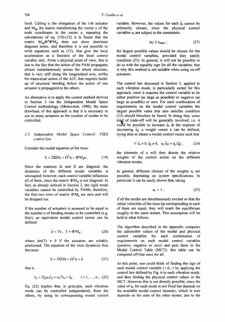
The block diagram of the model for the complete AJT control system is sketched in Fig. 14. Results of the simulation of the AJT control system are given in Fig. 15 (combined-mode excitation) and Fig. 16 (single-mode excitation). Initial conditions are the same as those used in Section 5.5 (simulations in ideal conditions). To ensure proper operation of the controller, it has been necessary to increase the velocity threshold from 1.5 to 2.0 mm/s. The control transients are somewhat longer than in the ideal case, due to the estimator's settling time.

0 . 2 i ,

0.1 - - 1 , i i = i Tip v e l o c i t y 0 ' " '

h L

0 1 2 3 4

. |ItRt : , Tip control-IOIIJkIIII'I~""I4LIJJII : : :

I , , ,

- 1 .51 ~ = i L 0 1 2 3 4 5

T i m e (s )

Fig. 15. Simulations of the complete AJT VSES control system, combined-mode excitation


0.2 ~ = • ,

Tip velocity ~ ,

_0.2 0 1 2 3 4 5

! 05 . . . . ii Tip controlii~

0 1 2 Time (s)

h

3 4 5

0.2 ~ ,

0.1 ~ , . , i Tip velocity 0 ~ - ~

'~ '"-o,t / /~ ~ ! i ! ° 2 r ~ ; i i

0 2 3 4 5

0 5 ; ' ' - Tip control 0 ' i :

-0.

. , -st - - i i , 0 2 3 4 5

Time (s)

0.2

0.1 Tip velocity 0 i

(m/s) -0.1

-°,21~ "

1,111,I,1,tll ' Tip control

.o tilt - 1 I

" 1 " 5 I . . . . . ~ , 0 1 2

Time (s)

! I

T

J

4 5

I

4 5

t ~ r 1 t o.2 , ; i :

Ti veocity O l ,m,s, o10 . . . . . 1 . o 2 ~ : i 1

0 1 3 4

1 ~ r

0,5 * Tip control 0 - _ "- 2

-o,5

0 1 2 3 4 Time (s)

Fig. 16. Simulations of the complete AJT VSES control system, single-mode excitation

0.2

0.1 Tip velocity 0

(m/s) -0.1

-0.2

100

50

u(1) 0

-50

-100

l T ' r

2 3 4 5

I

i 1

I 2 3 4 5 Time (s)

Tip velocity 0" 10 ~ 1 1 / ~ , ~ ~ , . , , ~ ~ - ! - , .

0 1 3 4 I

5o ', u(1) 0

-50

-100 i

1 3 4 5 Time (s)

o.2 0.1;

Tip velocity 0

(m/s) -0.1

-0.2

100

50

u(1)

-50 -100

i I T

I I

i

I 4

i ! 1

i i

3 4

I

;I i

3 4 Time (s)

02r i i : 0.1~- - , ~ ~

T~pve,o~ty 0 h : : : (m/s) [ w i i i

0 2

u , , ~ 11

0 2 Time (s)

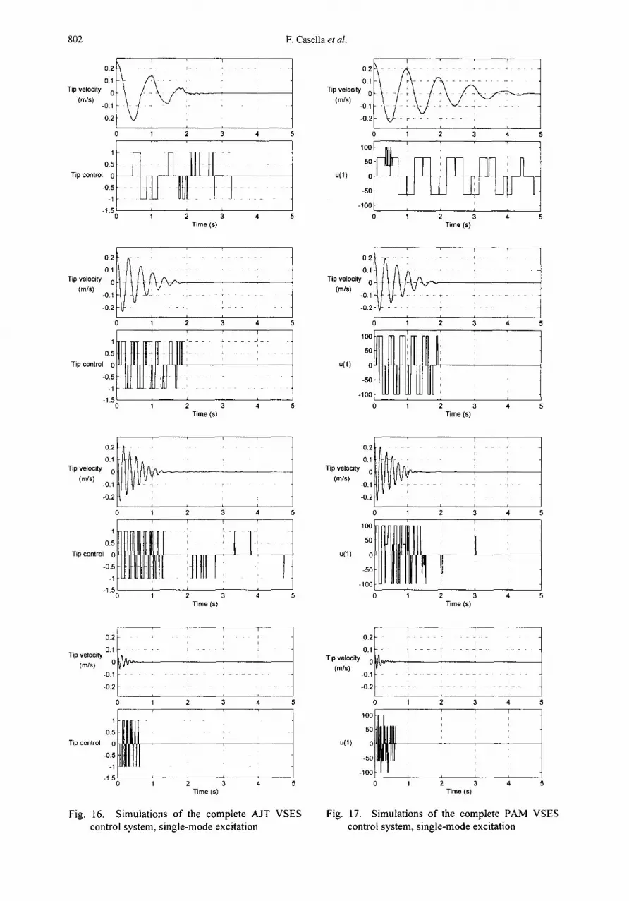
Fig. 17. Simulations of the complete PAM VSES control system, single-mode excitation


0.2 0.1

Tip velocity 0 (m/s)

-0.1

uO)

-0.2

0 1 i I i

1 2 3 4

100

50

0

-50

-100

o . 2 ~ _ A _ . L _ ' , . . . . ~ __i ::> .... : .

velocitY ~ ' ' '

- o q ~ - , - ; - •

0 1 2

0.5 Tip control 0 i

-o.s

-11 i 0 1 2

Time (s)

Time ($)

Fig. 18. Simulations of the c9mplete PAM VSES control system, combined-mode excitation

6. 4. Simulation of the complete PAM control system

Results of the simulation of the PAM control system with the usual initial conditions are given in Figs 17 and 18. The block diagram of the system is analogous to the one in Fig. 14, the only difference being the absence of the actuator delay. To ensure proper operation of the controller, it has been necessary to increase the velocity threshold from 1.0 to 2.0 mm/s of tip velocity for each vibration mode. Note that the ideal controller (Figures 11 and 12) has direct access to the state variables, and being based on the IMSC concept is such that, if one mode only is excited, the control variables will influence that mode only; here, instead, state estimates are used by the controller, and they are different from zero also for the other modes, due to the estimator's settling transient; the controller therefore acts accordingly, as if they had really been excited. This explains the spikes that can be observed when the first mode is excited, between .3 and .6 seconds, and the different control levels in the other cases.

0 1 ~ ~ - ~ . . . . . . . . . . . . . . 4 /

0

Ti° coo,, _o:s U Eli L -1.5 0

2 4 i

LI L

2 Time (s)

i ,

0.1 • ~ . ~ ~

Tip velocitY.o.2 -0.1 0 , ~ ~ , , ,

0 1 2 ' T r

'l]ll ltittqllll I iI l 0.5 i Tip control -0_.~0 ii I

: 0 1 2 3

Time (s)

7. EXPERIMENTAL RESULTS

The AJT controller has actually been implemented and tested in the laboratory (Casella and Gruppi, 1994, Bernelli-Zazzera, et al., 1995). Significant results are given in Figs 19 and 20. The initial conditions for the experiments are set by a mechanical excitation system, that brings the structure in a steady oscillation, with the maximum velocities relative to each mode approximately equal to those used in the simulations. When the excitator is disconnected from the structure, the control experiment begins: this means that the initial conditions are not exactly the same used for the simulations, since the initial phase of each mode is unknown; they are however equivalent from an energy point of view.

0 2 - ~ ~ - - ~ • -

/ /

Tip velodty 0 ~ ' ~ ~ ~ ~

-0.1 ~- ~ * i I I

-o2 F • ~ _ , L ~ i J i

0 1 2 3 4

II1[ [ILLLI ILl I;ILL ti;l Tip control 0 ~ r~ l~ l i: ,

o m,,rllll I111111I I -1 , i - 1 . 5 ~ ' ' ' ~ ; ~ ; ;

Time (s)

Fig. 19. Experimental results of the AJT VSES controller, single-mode excitation


0.2

0.1 Tip velocity 0

-0.1

-02

1

0.5

T ip~n t ro l 0

-0.5

-1

-1.5

i i i '

i i =

I J

1 2 3

,

i = I

1 2 3 Time (s)

4

T 4

J 5

Fig. 20. Experimental results of the AJT VSES controller, combined-mode excitation

frequency, unmodeled dynamics. Finally the AJT controller has also been successfully tested in the laboratory. Future research may consider the experimental validation of the PAM controller, the design of an integrated controller using both AJTs and PAMs, and the study of the control system response to external disturbances other than the simple disturbance on the initial conditions studied in this work.

APPENDIX: CALCULATION OF THE MCT

The algorithm described here finds the largest possible values of the modal control variables

= Tu, subject to the following constraints

iuil ~ Umax ; (33)

Note that it has been necessary to increase the velocity threshold of the controller to 2.5 mm/s. The velocity signals have been obtained from the experimental acceleration measurements by means of a Kalman filter; this was necessary to be able to remove the rigid mode velocity components. The velocity signals shown in Figures 19 and 20 are therefore significant only after the settling time for the filter has elapsed. With these considerations in mind, the experimental results fully confirm those obtained by simulation.

The control spikes that appear when the fourth mode is excited are due to the suspension springs, whose vibration mode is also excited, having a natural frequency (9.2 Hz) very close to that of the truss (8.9 Hz). In this case, the springs act as exogenous disturbance generators, since their motion is not controllable by the actuators. The controller then tries to counteract their effect until their motion ends by natural damping. This is the reason why the initial velocity of the tip has been kept smaller for the fourth mode than for the others.

For further details, the reader is referred to (Casella and Gruppi, 1994) and (Casella, e t al., 1995).

8. CONCLUSIONS

Two nonlinear controllers, based on a common principle, have been proposed for vibration suppression in a laboratory structure, representative of a real space-borne structure; these two controllers employ AJT and PAM actuators respectively. The resulting control systems have been tested by means of simulations, and it has been verified that, with the use of a suitable state estimator, good system performance can be achieved even in the presence of measurement noise, actuator delays and high

V ui ¢ 0, Uk ~ 0, ai [~il = ak I~kl ; (34)

for each combination of requirements on each modal control variables (i.e. positive, negative or zero); eq. (33) is the physical realisability constraint, while eq. (34) describes the relative weighting of the different modal control variables.

The algorithm is executed off-line, building the Modal Control Table (MCT), whose entries are all the combinations of requirements on the modal control variables. Subsequently, a simple table look- up is needed by the real-time controller to obtain the desired physical control variables in all cases.

The bi-dimensional case will be first examined graphically, for the sake of clarity; then the algorithm will be extended to the n-dimensional case.

Define the vector tx as

1 D ,

~i = ai ai ~: 0

c q = 0 , a i = 0 (35)

Figures 21a and 21b show the space of the modal control variable with two different values of the T transform matrix: the shaded area is the admissible region, where eq. (33) holds, while the two straight lines r, s represent the constraints:

Fig. 21. Modal control admissible values


+al Ul = +a2 U2 ; (36)

-a l Ul = +a2 fi2 ; (37)

If, for instance, fil > 0 and fi2 = 0 are required, point A will be chosen, that is the one that solves

max a* '

Uk = 0 V a k = 0

lUkl < Urea x V k = 1 ..... n ; u = T -1

max +~1 ~1 (38)

~2 = O. (39)

The actual physical control values will then be easily calculated via the inverse transform matrix T q.

In a case where Ul > 0 and ~2 < 0 are required, point B will be chosen, that is the one that solves:

max --~1 Ul + 0~2 U2 (40)

ai* ui = ak* Uk V i ¢ k I ui ¢ 0, Uk ¢ 0 (44)

and let u* = u.

3. For all the possible subsets o f the set o f constraints (44)

solve the problem of step 2 with the reduced set o f constraints

ifabs(uk) > abS(Uk*) V k = 1 ..... n

then fi* = ft.

-a l Ul = +a2 fi2 ; (41) 4. Let u = T "1 u*.

When fil > 0 and U2 > 0, things become less straightforward: in the case of Fig. 21a the required solution will be point C, i.e.:

max +a l fil + t:t2 u2 (42)

+al fil = +a2 u2 , (43)

while in the case of Fig. 21b it seems more reasonable to choose point D instead, i.e. the solution of eq. (42) without the constraint (43), since both its coordinates are greater than those of point C. In other words, only Pareto-optimal solutions should be considered, i.e. solutions that are not dominated by others.

Many of the constraints (44) are actually linearly dependent, and thus redundant; standard linear algebra methods can be exploited to extract the independent ones.

Step 3 should be performed by progressively removing the constraints, i.e. first examining the subset SI obtained by removing one constraint from (44), then the subset S 2 obtained by removing two constraints, and so on. Different solutions can be found, depending on the order in which the elements of each Si are examined; however, since none of them would dominate the others, the choice among them is arbitrary, and therefore any examination order for the elements of each Si subset is equally good.

The algorithm to compute the physical control variable vector u in the general n-dimensional case, given the requirements on the sign of the modal control variables, can now be sketched.

1. Build vectors a*, ct*, as

f +a k ifuk > 0 ak* = 0 i fu k = 0

- a k if Uk < 0

1 if~k > 0 ak

Ctk* = 0 i fu k = 0

- 1 i fuk < 0. ak

2. Solve the linear programming problem

A C K N O W L E D G E M E N T S

This paper has partially been supported by MURST (40% and 60% funds) and CNR (Centro Teoria dei Sistemi). The authors are grateful to Prof. Franco Bernelli-Zazzera and Prof. Amalia Ercoli-Finzi (Dipartimento di Ingegneria Aerospaziale), who have made this research possible, and to Marco Gruppi, who worked with the authors on the AJT controller design and experimental testing.

REFERENCES

Anderson, B. D. O. and J. B. Moore (1979). Optimal Filtering, pp. 105-115. Prentice-Hall.

Barbieri, E. and U. Ozguner (1988). Rest-to-Rest Slewing of Flexible Structures in Minimum


Time. Proceedings of the 27 th Conference on Decision & Control pp. 1633-1638.

Bashein, G. (1971). A Simplex Algorithm for On- Line Computation of Time Optimal Controls. IEEE Transactions on Automatic Control AC- 16, pp. 479-482.

Ben-Asher, J., J. A. Bums and E. M. Cliff (1987). Time Optimal Slewing of Flexible Spacecraft. Proceedings of the 26 th Conference on Decision & Control, pp. 524-528.

Bernelli-Zazzera F., F. Casella, A. Ercoli-Finzi, A. Locatelli and N. Schiavoni (1995). Modified Discrete-Time Velocity Feedback for Vibration Suppression of a LSS Laboratory Model, Proceedings of the 10 th VPI&SU Symposium on Dynamics and Control of Large Structures, Blacksburg-Virginia.

Bemelli-Zazzera F., D. Cristiani, A. Ercoli-Finzi, A. Guidotti, A. Locatelli and N. Schiavoni (1993). A Study on Nonlinear Control of Space Structures Using Active Members and Jet Thrusters. Proceedings of the 9 th VPI&SU Symposium on Dynamics and Control of Large Structures, Blacksburg-Virginia, pp. 505-516.

Bernelli-Zazzera F. and P. Mantegazza (1993). An Experiment on Active Control of Large Space Structures by Means of Jet Thrusters. Proceedings of the 12 th AIDAA Conference, Como, Italy, pp. 1139-1147.

Blanchini, F., (1992). Minimum Time Control for Uncertain Discrete-Time Linear Systems. Proceedings of the 31 st Conference on Decision & Control, pp. 2629-2634.

Casella F. and M. Gruppi (1994). Progetto e Sperimentazione di un Sistema di Controllo Mediante Attuatori a Getto delle Vibrazioni di una Grande Struttura Flessibile. Graduation thesis (in italian), Politecnico di Milano, Italy.

Casella F., A. Locatelli and N. Schiavoni (1995). Nonlinear Controllers for Vibration Suppression in a Large Flexible Structure. Internal report 027-95, Dipartimento di Elettronica e Informazione, Politecnico di Milano, Italy.

Cristiani D. and A. Guidotti (1992). Simulazione e Controllo delle Vibrazioni di un Modello di Laboratorio di una Grande Struttura Spaziale. Graduation Thesis, Politecnico di Milano, Italy.

De Santis, R. M. and S. De Santis (1992). A Bang- Bang Controller for Vibration Reduction in a Rotating Flexible Beam. Proceedings of the 31 st Conference on Decision & Control pp. 3123- 3125.

DeVlieger, J. H., H. B. Verbruggen and P. M. Bruijn (1982). A Time Optimal Control Algorithm for Digital Computer Control. Automatica 18, pp. 239-244.

Dodds, S. J. and S. E. Williamson (1984). A Signed Switching Time Bang-Bang Attitude Control Law for Fine Pointing of Flexible Spacecraft. International Journal of Control 40, pp. 795- 811.

Ercoli-Finzi A., D. Gallieni and S. Ricci (1993). Design, Modal Testing and Updating of a Large Space Structure Laboratory Model (TESS). Proceedings of the 9 th VPI&SU Symposium on Dynamics and Control of Large Structures, Blacksburg-Virginia, pp.409-420.

Juang, J.N. and D. W. Sparks (1992). Survey of Experiments and Experimental Facilities for Control of Flexible Structures. Journal of Guidance, Control and Dynamics 15, pp. 801- 816

Keerthi, S. S. and E. G. Gilbert (1987). Computation of Mininum-Time Feedback Control Laws for Discrete-Time Systems with State-Control Constraints. IEEE Transactions on Automatic Control AC-32, pp. 432-435.

Knudsen, H. K. (1964). An Iterative Procedure for Computing Time-Optimal Controls. IEEE Transactions on Automatic Control AC-9, pp. 23-30.

Meirovitch, L. (1990). Dynamics and Control of Structures, J. Wiley & Sons.

Pao, L. Y. and G. F. Franklin (1990). Time-Optimal Control of Flexible Structures. Proceedings of the 29 th Conference on Decision & Control pp. 2580-2581

Pao, L. Y. and G. F. Franklin (1992). Robustness Studies of a Proximate Time-Optimal Controller. Proceedings of the 31 st Conference on Decision & Control pp. 3559-3564.

Singh, G., P. T. Kabamba and N. H. McClamroch (1989). Planar, Time-Optimal, Rest-to-Rest, Slewing Maneuvers of Flexible Spacecraft. Journal of Guidance, Control & Dynamics 12, pp. 71-81.

Thompson, R. C., J. L. Junkins and S. R. Vadali (1989). Near Minimum Time Open Loop Slewing of Flexible Vehicles. Journal of Guidance, Control & Dynamics 12, pp. 82-88.

Vander Veide, W., E. and J. He (1983). Design of Space Structure Control System Using On-Off Thrusters. Journal of Guidance, Control & Dynamics 6, pp. 53-60.

Documents

Nonlinear controllers for vibration suppression in a large flexible structure