Multivariate Student-t Regression Models:

Pitfalls and Inference

By Carmen Fernandez and Mark F.J. Steel 1

CentER for Economic Research and Department of EconometricsTilburg University, 5000 LE Tilburg, The Netherlands

FIRST VERSION DECEMBER 1996; CURRENT VERSION JANUARY 1997

Abstract

We consider likelihood-based inference from multivariate regression models with in-dependent Student-t errors. Some very intruiging pitfalls of both Bayesian and classicalmethods on the basis of point observations are uncovered. Bayesian inference may beprecluded as a consequence of the coarse nature of the data. Global maximization of thelikelihood function is a vacuous exercise since the likelihood function is unbounded as wetend to the boundary of the parameter space. A Bayesian analysis on the basis of setobservations is proposed and illustrated by several examples.

KEY WORDS: Bayesian inference; Coarse data; Continuous distribution; Maximum like-lihood; Missing data; Scale mixture of Normals.

1. INTRODUCTION

The multivariate regression model with unknown scatter matrix is widely used inmany fields of science. Applications to real data often indicate that the analytically con-venient assumption of Normality is not quite tenable and thicker tails are called for inorder to adequately capture the main features of the data. Thus, we consider regressionerror vectors that are distributed as scale mixtures of Normals. We shall mainly emphasizethe empirically relevant case of independent sampling from a multivariate Student-t distri-bution with unknown degrees of freedom. In particular, we provide a complete Bayesian

1 Carmen Fernandez is Research Fellow, CentER for Economic Research and Assistant Professor, De-partment of Econometrics, Tilburg University, 5000 LE Tilburg, The Netherlands. Mark Steel is SeniorResearch Fellow, CentER for Economic Research and Associate Professor, Department of Econometrics,Tilburg University, 5000 LE Tilburg, The Netherlands. We gratefully acknowledge the extremely valu-able help of F. Chamizo in the proof of Theorem 3 as well as useful comments from B. Melenberg andW.J. Studden. Both authors benefitted from a travel grant awarded by the Netherlands Organization forScientific Research (NWO) and were visiting the Statistics Department at Purdue University during muchof the work on this paper.

2

analysis of the linear Student-t regression model, and also comment on the behaviour ofthe likelihood function.

The Bayesian model will be completed with a commonly used improper prior on theregression coefficients and scatter matrix, and some proper prior on the degrees of freedom.Section 3 examines the usual posterior inference on the basis of a recorded sample of pointobservations. Even though Theorem 1 indicates that Bayesian inference is possible foralmost all samples (i.e. except for a set of zero probability under the sampling model),problems can occur since any sample of point observations formally has probability zero ofbeing observed. In practice, this can become relevant due to rounding or finite precision ofthe recorded observations, and we can easily end up with a sample for which inference isprecluded. This incompatibility between the continuous sampling model and any sample ofpoint observations can have very disturbing consequences: the posterior distribution maynot exist, even if it already existed on the basis of a subset of the sample. New observationscan, thus, have a devastating effect on the usual Bayesian inference. Fernandez and Steel(1996a) present a detailed discussion of this phenomenon in the context of a univariatelocation-scale model.

Section 4 presents a solution through the use of set observations, which have positiveprobability under the sampling model, and are, thus, in agreement with the samplingassumptions. This leads to a fully coherent Bayesian analysis where new observationscan never harm the possibility of conducting inference. A Gibbs sampling scheme [seee.g. Gelfand and Smith (1990) and Casella and George (1992)] is seen to be a convenientway to implement this solution in practice. Some examples are presented: a univariateregression model for the well-known stackloss data [see Brownlee (1965)], and a bivariatelocation-scale model for the iris setosa data of Fisher (1936).

The analysis through set observations is naturally extended to the case where somecomponents of the multivariate response are not observed (missing data). We illustratethis with the artificial Murray (1977) data, extended with some extreme values in Liu andRubin (1995).

In addition, we find that none of the results concerning the feasibility of Bayesianinference with set observations depend on the particular scale mixture of Normals that wesample from.

Finally, in Section 5 the Student likelihood function for point observations is analyzedin some detail: it is found that the likelihood is unbounded as we tend to the boundaryof the parameter space in a certain direction. This casts some doubt on the meaning andvalidity of a maximum likelihood analysis of this model [as performed in e.g. Lange, Littleand Taylor (1989), Lange and Sinsheimer (1993) and Liu and Rubin (1994, 1995)]. Thisbehaviour of the likelihood function is illustrated through the stackloss data example, andit also explains the source of the problems encountered by Lange et al. (1989) and Langeand Sinsheimer (1993) when applying the EM algorithm for joint estimation of regressioncoefficients, scale and degrees of freedom to the radioimmunoassay data set of Tiede andPagano (1979).

All proofs are grouped in Appendix A, whereas Appendix B recalls some matricvariateprobability densities used in the body of the paper. With some abuse of notation, we do notexplicitly distinguish between random variables and their realizations, and p(·) (a density

3

function) or P (·) (a measure) can correspond to either a probability measure or a generalσ-finite measure. All density functions are Radon-Nikodym derivatives with respect to theLebesgue measure in the corresponding space, unless stated otherwise.

2. THE MODEL

Observations for the p-variate response variable yi are assumed to be generated throughthe linear regression model

yi = β′xi + εi, i = 1, . . . , n, (2.1)

where β is a k × p matrix of regression coefficients, xi is a k-dimensional vector of ex-planatory variables and the entire design matrix, X = (x1, . . . , xn)′, is taken to be offull column rank k [denoted as r(X) = k]. The error vectors εi are independent andidentically distributed (i.i.d.) as p-variate scale mixtures of Normals with mean zero andpositive definite symmetric (PDS) covariance matrix Σ. The mixing variables, denoted byλi, i = 1, . . . , n, follow a probability distribution Pλi|ν on <+, which can depend on a pa-rameter ν ∈ N (possibly of infinite dimension). Thus, we have n independent replicationsfrom the sampling density

p(yi|β,Σ, ν) =

∫ ∞0

λp/2i

(2π)p/2|Σ|1/2exp

−λi

2(yi − β

′xi)′Σ−1(yi − β

′xi)

dPλi|ν . (2.2)

By changing Pλi|ν we cover the class of p-variate scale mixtures of Normals. The latter is asubset of the elliptical class [see Fang, Kotz and Ng (1990), chap. 2], with ellipsoids in <p

as isodensity sets, while allowing for a wide variety of tail behaviour. Leading examples arefinite mixtures of Normals, corresponding to a discrete distribution on λi, and multivariateStudent-t distributions with ν > 0 degrees of freedom, where Pλi|ν is a Gamma distributionwith unitary mean and both shape and precision parameters equal to ν/2. Most of thesubsequent discussion will focus on the empirically relevant case of Student-t sampling.

Special cases of the model in (2.1) are the multivariate location-scale model, wherek = 1 and xi = 1, and the univariate regression model for p = 1.

The Bayesian model needs to be completed with a prior distribution for (β,Σ, ν). Inparticular, we assume a product structure between the three parameters where

p(β,Σ) ∝ |Σ|−(p+1)/2 (2.3)

andPν is any probability measure on N . (2.4)

The prior in (2.3) is the “usual” default prior in the absence of compelling prior informationon (β,Σ). Under fixed ν it corresponds to the Jeffreys’ prior under “independence” and isthus invariant under separate reparameterizations of β and of Σ.

Note that the model in (2.1) implies that all p components of yi are regressed on thesame variables xi. Thus, we treat a special case of Zellner’s (1962) seemingly unrelated

4

regression (SUR) model, which allows for different regressors on the p components. Al-ternatively, our framework can be extended to general SUR models by considering priorsthat impose zero restrictions on certain elements of β.

3. BAYESIAN INFERENCE USING POINT OBSERVATIONS

We now consider the feasibility of a Bayesian analysis of the model in (2.2)− (2.4) onthe basis of the recorded point observations, as is the usual practice. Since the prior in(2.3) is improper, we clearly need to verify the existence of the posterior distribution. Thefollowing Theorem addresses this issue.

Theorem 1. Consider n independent replications from (2.2) with any mixing distributionPλi|ν and the prior in (2.3)− (2.4) with any proper Pν. Then the conditional distributionof (β,Σ, ν) given y ≡ (y1, . . . , yn)′ exists if and only if n ≥ k + p.

Somewhat surprisingly, neither the mixing distribution nor the prior on ν affects theexistence of the conditional distribution of the parameters given the observables (i.e. theposterior distribution). Thus, whenever n ≥ k+ p, the fact that the prior is improper is ofno consequence for the existence of the posterior distribution. However, probability theorytells us that a conditional distribution is only defined up to a set of measure zero in theconditioning variables. In other words, Theorem 1 assures us that p(y) <∞ except possiblyon a set of Lebesgue measure zero in <n×p. Theoretically, this validates inference sinceproblems can only occur for samples that have zero probability of being observed. However,as stressed in Fernandez and Steel (1996a), any recorded sample of point observations haszero probability of occurrence under any continuous sampling distribution. Thus, Theorem1 does not guarantee that p(y) < ∞ for our particular observed sample, and the latterhas to be verified explicitly. Note that this problem stems from an inherent violation ofthe rules of probability calculus, since the recorded observations are in contradiction withthe assumed sampling model, and is in no way linked to the improperness of the prior [seeFernandez and Steel (1996a) for a more detailed discussion].

If we complement Theorem 1 by considering any possible point y ∈ <n×p, Lemma 1in the Appendix shows that both Pλi|ν and Pν can intervene. It is immediate from Lemma1 that

for finite mixtures of Normals, p(y) <∞ if and only if r(X : y) = k + p, (3.1)

which is the minimal possible requirement for any scale mixture of Normals. In the sequelof this Section, we shall, therefore, assume that this rank condition holds.

Let us now analyze the more challenging case of Student-t sampling, where we shalluse the following Definition:

Definition 1. For a design matrix X and a sample y ∈ <n×p, sj , j = 1, . . . , p, is thelargest number of observations such that the rank of the corresponding submatrix of X isk while the rank of the corresponding submatrix of (X : y) is k + p− j.

Clearly, since r(X : y) = k + p, we obtain that k ≤ sp < sp−1 < . . . < s1 < n. Nowwe can present the following Theorem.

5

Theorem 2. Let y = (y1, . . . , yn)′ be a sample of n independent replications from a p-variate Student-t distribution in (2.2), and consider the prior in (2.3) − (2.4). Assumingthat r(X : y) = k + p and defining

m = maxj=1,...,p

jn− k

n− sj− p

,

while recalling Definition 1 for s1, . . . , sp, we obtain that(i) if m = 0, then p(y) <∞;(ii) if m > 0, then p(y) <∞ if and only if

Pν(0,m] = 0 and

∫ m+ρ

m

(ν −m)−qdPν <∞, for all ρ > 0,

where q denotes the number of indices j ∈ 1, . . . , p for which m = j n−kn−sj

− p.

From Definition 1 we note that sj = k+ p− j (which implies m = 0), for all y ∈ <n×p

excluding a set of Lebesgue measure zero. Thus, Theorem 2 (i) will apply and inferenceis feasible with almost all samples, as was already clear from Theorem 1. However, aswill be illustrated in the Examples in Section 4, observed samples often lead to valuesof m > 0, as a consequence of rounding or the finite precision of the measuring device.Then, Theorem 2 (ii) indicates that the prior for ν can not put any mass on values ofν ≤ m. As an immediate consequence, inference based on samples for which m > 0is precluded under any prior Pν with support including (0,K) for some K > 0. Thisnegative result even extends to improper priors for ν. Thus, popular choices for Pν suchas the improper Uniform on <+, Jeffreys’ prior [Liu (1995)] or distributions in the Gammafamily [Geweke (1993)] can never lead to a posterior distribution whenever m > 0 for theparticular sample of point observations under consideration. Bounding ν away from zeroby some fixed constant [as in Relles and Rogers (1977) or Liu (1995, 1996)] provides nogeneral solution either, since m is typically updated as sample size grows and can reach anupper bound of n− k− p (when s1 = n− 1). This continual updating of m has the rathershocking consequence that adding new observations can actually destroy the properness ofa posterior which was proper with the previous sample!

In the special case of univariate regression (p = 1), the quantity m in Theorem 2simplifies to m = (s1 − k)/(n − s1) where s1 is the largest number of observations suchthat both the corresponding submatrix of X and the corresponding submatrix of (X : y)have rank k. Now, s1 ≥ k will have the interpretation of the largest possible number ofobservations for which yi can be fitted exactly by β′xi for some fixed value of β. Of course,q introduced in Theorem 2 (ii) is one in this case.

If we further specialize to k = 1 and take xi = 1, we are in the univariate location-scale model analyzed in Fernandez and Steel (1996a). Then, m becomes (s1− 1)/(n− s1),where s1 is the largest number of observations that are all the same. In that case, as soonas the sample contains repeated observations, a Bayesian analysis on the basis of pointobservations is precluded if the support of Pν is not bounded away from zero.

6

4. BAYESIAN INFERENCE USING SET OBSERVATIONS

A formal solution to the problem mentioned in Section 3 is to consider set observationswhich have positive probability under the continuous sampling model. In practice, itseems natural to consider a neighbourhood Si of the recorded point observation yi on thebasis of the precision of the measuring device. This avoids the incompatibility betweenobservations and sampling assumptions and, under a proper prior, posterior inference isalways guaranteed. For the improper prior in (2.3)− (2.4) a formal examination leads tothe following Theorem:

Theorem 3. Consider the Bayesian model (2.2)−(2.4) and n compact sets Si, i = 1, . . . , n,of positive Lebesgue measure in <p. Then P (y1 ∈ S1, . . . , yn ∈ Sn) < ∞ if and only ifr(X : y) = k + p for all y1 ∈ S1, . . . , yn ∈ Sn.

Remark that neither the mixing distribution Pλi|ν nor the prior of ν, Pν , intervene inTheorem 3, which thus holds for any scale mixture of Normals. Now Bayesian inference isfully coherent and adding extra observations can never destroy the possibility of conductinginference.

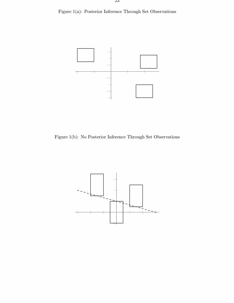
The condition r(X : y) = k+ p, which was always necessary under point observations[see (3.1)], becomes both necessary and sufficient when extended to sets as in Theorem 3.In the case of a location-scale model (k = 1 and xi = 1), the latter condition is equivalentto the absence of a (p − 1)-dimensional affine space that intersects with all of the setsS1, . . . , Sn. Figure 1 graphically illustrates this issue in the bivariate case (p = 2): whilethe set observations in Figure 1 (a) allow for posterior inference, the latter is precluded inFigure 1 (b).

In general, Bayesian inference using set observations can easily be implemented througha Gibbs sampler on the parameters augmented with y = (y1, . . . , yn)′. We then conditionon the set observations y1 ∈ S1, . . . , yn ∈ Sn, which shall, for convenience, be denotedas y ∈ S. Let us present this in more detail for Student-t sampling. In this case, it willprove convenient to also augment with the mixing variables λ = (λ1, . . . , λn)′ introducedin (2.2), leading to the following full conditionals:

p(y|β,Σ, ν, λ, y ∈ S) ∝ fn×pMN (y|Xβ,Σ⊗ Λ−1)IS(y), (4.1)

where we have used the notation for a matricvariate Normal explained in Appendix B,Λ = diag(λ1, . . . , λn) and IS(·) denotes the indicator function of the set S. Note that from(4.1) the yi’s are independently drawn from p-variate Normal distributions with mean β′xiand covariance matrix λ−1

i Σ, truncated to the relevant sets Si.The second conditional is

p(β,Σ|ν, y, λ, y ∈ S) = fk×pMN (β|β,Σ⊗ (X ′ΛX)−1)fpIW (Σ|Σ, n− k), (4.2)

i.e. the product of a matricvariate Normal and an Inverted Wishart density function (as

defined in Appendix B), where β = (X ′ΛX)−1X ′Λy and Σ = y′Λ−ΛX(X ′ΛX)−1X ′Λy.

7

The conditional distribution of ν is absolutely continuous with respect to Pν withRadon-Nikodym derivative proportional to

(ν2

)nν/2 Γ(ν

2

)−nexp

−ν

2

n∑i=1

(λi − log λi)

. (4.3)

For exponential Pν (as used in the Examples below), drawings from this non-standarddistribution can be generated following Geweke (1994) and Fernandez and Steel (1996b).

Finally, n independent Gamma distributions constitute the required conditional forλ:

p(λ|β,Σ, ν, y, y ∈ S) =n∏i=1

fG

(λi∣∣ν + p

2,ν + (yi − β′xi)′Σ−1(yi − β′xi)

2

), (4.4)

where fG(λi|a, b) ∝ λa−1i exp(−bλi) denotes the probability density function (p.d.f.) of a

Gamma distribution.Using the Gibbs sampler in (4.1) − (4.4), we can easily analyze the following three

Examples under Student-t sampling with the prior in (2.3)− (2.4). In all cases, we takePν to be exponential with mean 10 and variance 100, i.e.

p(ν) = fG(ν|1, 1/10), (4.5)

which spreads the prior mass over a wide variety of tail behaviour. Throughout, resultsare based on 250,000 Gibbs drawings with a burn-in of 10,000.

We start with a univariate regression model:

Example 1. Stackloss dataThis classical data set, originally presented in Brownlee (1965), has been subjected to

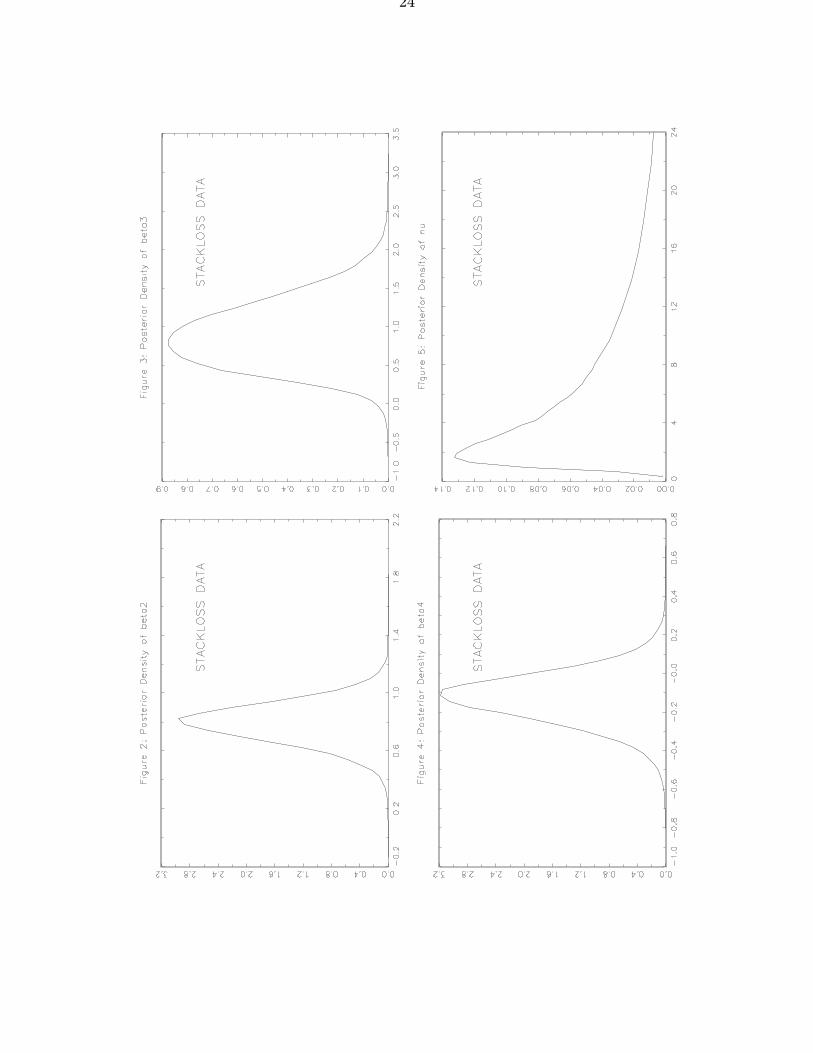
numerous robust methods [e.g. Andrews (1974) and Rousseeuw and van Zomeren (1990)]and was treated under Student-t sampling by Lange et al. (1989) in a classical maximumlikelihood framework. The data consist of n = 21 observations of a univariate response(stackloss) given an intercept and three other regressors. Thus, p = 1 and k = 4. RecallingDefinition 1, we can derive that for this data set s1 = 8, which means that we can fit eightobservations yi by β′xi for a certain value of β ∈ <4, namely β = (−36, 0.5, 1, 0)′. Thus,m in Theorem 2 takes the value (s1 − k)/(n − s1) = 4/13, precluding Bayesian inferenceon the basis of these point observations under Student sampling with the prior in (2.3),(2.4) and (4.5).

Here, we shall conduct inference through set observations in accordance with the preci-sion implicit in the number of digits recorded. We have verified that these set observationsfulfill the condition stated in Theorem 3, thus allowing for a Bayesian analysis. Figures2-5 summarize the posterior inference on the regression coefficients β2, . . . , β4 (excludingthe intercept) and the degrees of freedom ν.

The mixing variables λi in (2.2) can be seen as observation-specific precision factors, sothat unusually small values of λi correspond to “outlying” observations. The EM algorithmused in Lange et al. (1989) takes the mean of the conditional distribution of λi in (4.4) as

8

the weight of observation i [see also Pettitt (1985) and West (1984)]. On the basis of theseweights Lange et al. (1989) identify observations 21, 4, 3 and 1 as outliers, like in the leastsquares analysis of Daniel and Wood (1971) and the robust analysis of Andrews (1974).In a Bayesian setup, we naturally focus on the marginal posterior distribution of the λi’sand find indeed that the posterior means for these four observations are considerably lowerthan that for the others. However, we also note that the posterior distributions of the λi’sdisplay a substantial spread. •

The second example is a multivariate location-scale model:

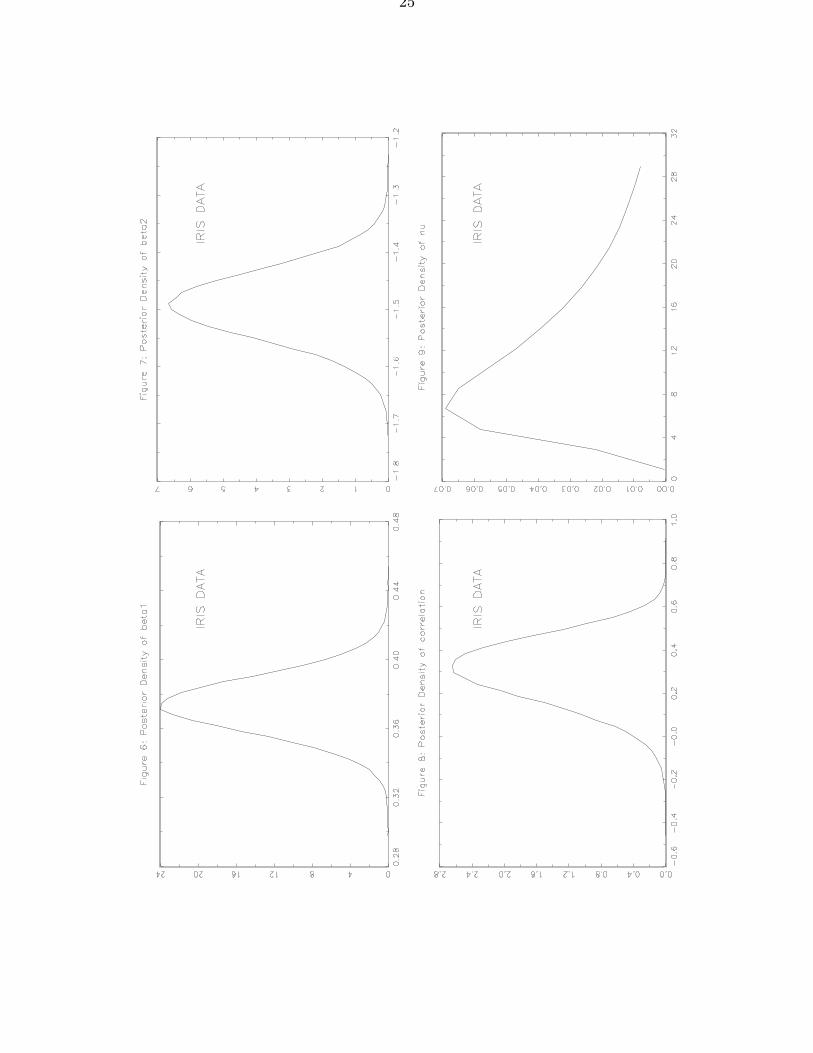
Example 2. Fisher’s Iris data

This data set, consisting of n = 50 bivariate measurements (of petal length andwidth) for Iris setosa, was analyzed in Fisher (1936) and Heitjan (1989). These data willsimply be modelled as a bivariate location-scale model; thus, p = 2, k = 1 and xi = 1.The original measurements were transformed to logarithms [as suggested in Gnanadesikan(1977) and Heitjan (1989)] and the set observations were transformed accordingly. Heitjan(1989) advocates the use of grouped likelihood for this example and maximizes a Normallikelihood integrated over the respective sets Si (i = 1, . . . , n). For these data, we caneasily ascertain that s1 = 35 and s2 = 29 (see Definition 1), which implies that m = 8/3and, thus, Theorem 2 (ii) again indicates that point observations can not form the basisof a Bayesian analysis under Student sampling with the prior (2.3), (2.4) and (4.5).

The use of set observations leads to the posterior densities plotted in Figures 6-9,where “correlation” denotes the off-diagonal element of Σ divided by the square root ofthe product of the diagonal elements. Posterior inference is quite close to Heitjan’s classicalresults. •

A natural extension of our context of set observations is that of missing observations.In a classical analysis of this problem, the EM algorithm was introduced in Dempster, Lairdand Rubin (1977), while Bayesian approaches rely on data augmentation [see Tanner andWong (1987)] or imputation methods [e.g. Rubin (1987) and Kong, Liu and Wong (1994)].

Whereas, sofar, we considered observations consisting of bounded sets Si, the factthat some components of yi are missing implies that the corresponding set observationbecomes unbounded (in the direction of each missing component). Let us now examinethe case where r < n observations lead to compact sets, while n− r observations containunobserved elements.

Theorem 4. Consider the Bayesian model in (2.2) − (2.4). The observations consist ofr < n compact sets S1, . . . , Sr, whereas Sr+1, . . . , Sn are unbounded due to missing com-ponents. All n sets have positive Lebesgue measure in <p. Defining X(r) = (x1, . . . , xr)′

and y(r) = (y1, . . . , yr)′, we obtain:

(i) if r(X(r) : y(r)) = k+p, for all y1 ∈ S1, . . . , yr ∈ Sr, then P (y1 ∈ S1, . . . , yn ∈ Sn) <∞;(ii) if we can find values y1 ∈ S1, . . . , yn ∈ Sn for which r(X : y) < k + p, thenP (y1 ∈ S1, . . . , yn ∈ Sn) =∞.

From Theorems 3 and 4 (i) we immediately deduce that whenever the compact setobservations S1, . . . , Sr lead to a proper posterior, the same holds if we add the unboundedset observations Sr+1, . . . , Sn (corresponding to missing data). Clearly, adding observations

9

that do not contradict the sampling model can never destroy the existence of an alreadywell-defined posterior distribution.

Theorem 4 (ii) addresses the situation where the compact set observations do not resultin a posterior [since r(X(r) : y(r)) < k + p for some y(r)], and establishes the necessity ofr(X : y) = k + p for all y1 ∈ S1, . . . , yn ∈ Sn, for conducting Bayesian inference. In otherwords, Theorem 4 (ii) says that the necessary condition stated in Theorem 3 for compactsets extends to any sample of sets S1, . . . , Sn (possibly unbounded).

As explained in the discussion of Theorem 3, the assumption of Theorem 4 (ii) is mosteasily interpreted in the location-scale case (k = 1 and xi = 1), where r(X : y) < 1 + pmeans that there exists a (p − 1)-dimensional affine space that intersects all of the setsS1, . . . , Sn. Note that if we can find one such space that, in addition, intersects with allp coordinate axes, any new set corresponding to missing data will necessarily have anintersection with this (p − 1)-dimensional affine space. Thus, adding any number of setscorresponding to observations with missing components can never result in a posteriordistribution. Figure 10 graphically illustrates this point in the bivariate case (p = 2).

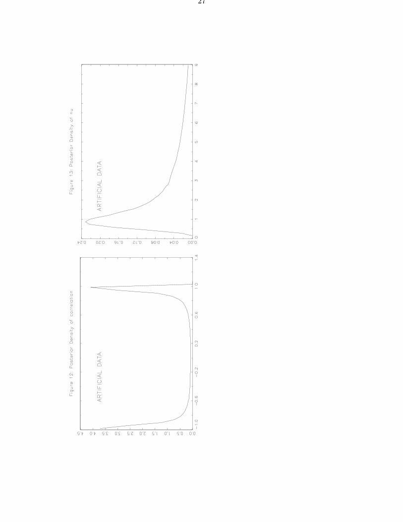
Example 3. Extended Murray data

In this Example, we focus on the artificial data originally introduced by Murray (1977)and extended with four extreme values in Liu and Rubin (1995). This results in thefollowing bivariate data set:

yi1 −1 −1 1 1 −2 −2 2 2 ? ? ? ? −12 12 ? ?yi2 −1 1 −1 1 ? ? ? ? −2 −2 2 2 ? ? −12 12

(4.6)

where n = 16, p = 2 and ? denotes a missing value. We use a location-scale model underStudent-t sampling, as in the maximum likelihood analysis of Liu and Rubin (1995) andthe Bayesian analysis of Liu (1995). Here, Bayesian inference will be conducted under theprior (2.3), (2.4) and (4.5), using set observations with a unitary width for the observedcomponents.

Figure 11 depicts the four compact sets (corresponding to the first four observations),and from Theorem 4 (i) we can immediately deduce properness of the posterior as no singleline can cross all four sets S1, . . . , S4. Note that deleting any one of these compact setobservations would result in an improper posterior [see Theorem 4 (ii) and the discussionthereafter] as the dashed line in Figure 11 indicates. Figures 12-13 plot posterior p.d.f.’sfor the correlation (as defined in Example 2) and the degrees of freedom ν. Compared tothe same analysis on the basis of the original Murray data [i.e. the first twelve in (4.6)],the correlation is more extreme and degrees of freedom tend to be substantially smaller.As expected, the analysis based on all sixteen set observations identifies the four extraobservations [i.e. the last four in (4.6)] as outliers through small values of the mixingvariables λi associated with these observations. In addition, we have found that inferencewith this model is remarkably insensitive with respect to the width chosen for the setobservations (in directions where they are bounded). •

10

5. THE STUDENT-t LIKELIHOOD FUNCTION

In this Section, we examine some peculiarities of the likelihood function correspondingto independent Student-t sampling in a general regression context. We shall only focuson the use of point observations, and present some classical counterparts of the problemsdescribed in Section 3 under a Bayesian treatment of this model.

In particular, we consider n replications from the following sampling density functionfor yi ∈ <p:

p(yi|β,Σ, ν) =Γ(ν + p)/2

Γ(ν/2)(πν)p/2|Σ|1/2

[1 +

1

νyi − gi(β)′Σ−1yi − gi(β)

]−(ν+p)/2

, (5.1)

where β ∈ B and gi(·) is a known continuous function from B to <p, possibly dependingon regressors xi. Thus, we extend the linear regression context of the previous Sections tomore general regression functions.

We shall reparameterize the PDS matrix Σ as (σ, V ) through

Σ = σ2V, (5.2)

where σ ∈ <+ and V ∈ Cp1 , which will denote the space of p×p PDS matrices with element(1, 1) equal to one. This reparameterization is useful for presenting the main result of thisSection.

Theorem 5. Let l(β, σ, V, ν) be the likelihood function corresponding to n independentreplications from (5.1) with the reparameterization in (5.2). Then:(i) l(β, σ, V, ν) is a finite continuous function in the entire parameter space B × (0,∞) ×Cp1 × (0,∞).(ii) For given values β = β0, V = V0 and ν = ν0, let 0 ≤ s(β0) ≤ n be the number ofobservations for which yi = gi(β0). We obtain:(iia)

if ν0 <s(β0)p

n− s(β0), then lim

σ→0l(β0, σ, V0, ν0) =∞;

(iib)

if ν0 =s(β0)p

n− s(β0), then lim

σ→0l(β0, σ, V0, ν0) ∈ (0,∞);

(iic)

if ν0 >s(β0)p

n− s(β0), then lim

σ→0l(β0, σ, V0, ν0) = 0.

From Theorem 5, whenever we can find a value β0 such that yi = gi(β0) holds forat least one observation, the likelihood function does not possess a global maximum. In-deed, for small enough values of ν [see (iia)], we can make l(β0, σ, V0, ν0) arbitrarily largeby letting σ tend to zero. Note that, in practice, we can typically find values β0 such

11

that s(β0) > 0. For example, in the case of p-variate linear regression with k regressors(considered in the previous Sections), we can deduce from Definition 1 that

maxβ∈<k×p

s(β) = sp ≥ k, (5.3)

thus precluding global maximization of the likelihood function, irrespectively of the sample.This finding casts some doubt on maximum likelihood (ML) estimation under Student-

t regression models with unknown degrees of freedom ν. In the existing literature, ν istypically allowed to vary in <+ [see e.g. Lange et al. (1989) and Lange and Sinsheimer(1993)]. Reported ML estimates must, therefore, correspond to local and not to globalmaxima, although this is not stated in these papers. To our knowledge, the existenceand uniqueness of such local maxima and the asymptotic properties of the correspondingestimators have not been formally established in the literature. In a pure location-scalecontext with fixed degrees of freedom, constrained to be sufficiently large, Maronna (1976)proves that the likelihood equations have a unique solution that leads to a consistent andasymptotically Normal estimator of (β,Σ). However, we have not encountered similarresults for unknown ν.

We remind the reader that a Bayesian analysis of the linear regression model basedon point observations breaks down if we assign prior probability to values of ν ≤ m, wherem is defined in Theorem 2. From Theorem 5 (ii) with (5.3) the likelihood is unbounded ifν < spp/(n−sp), which can generally be larger or smaller than m. In the case of univariatelinear regression (p = 1), the latter quantity becomes s1/(n − s1), which is always largerthan m = (s1 − k)/(n − s1). Thus, in this case, the likelihood is still integrable with theprior in (2.3)− (2.4) if Pν bounds ν strictly away from (s1− k)/(n− s1) (Theorem 2), butis unbounded for values of ν smaller than s1/(n−s1). Furthermore, there is a fundamentaldifference between classical and Bayesian results: as remarked in the discussion of Theorem2, m equals zero for all y ∈ <n×p except for a set of Lebesgue measure zero, implying thata Bayesian analysis is feasible for almost all samples (see also Theorem 1). In practiceproblems only occur due to the coarse nature of observed data. From Theorem 5 (iia) and(5.3), on the other hand, it is immediately clear that global maximization of the likelihoodis precluded for any sample y ∈ <n×p.

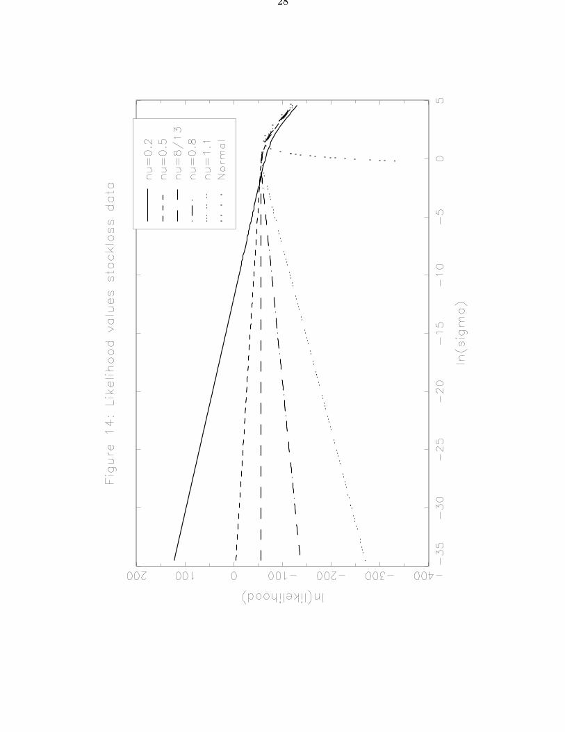
In order to illustrate the behaviour of the likelihood function, let us reconsider Exam-ple 1.

Example 1. (continued) Stackloss dataAs explained in Example 1, the value β0 = (−36, 0.5, 1, 0)′ allows us to exactly fit

eight of the 21 observations. Thus, from Theorem 5 (iia), taking ν0 < 8/13 leads tolimσ→0 l(β0, σ, 1, ν0) =∞ (note that p = 1 implies V0 = 1).

Figure 14 plots the logarithm of l(β0, σ, 1, ν0) as a function of the logarithm of σ, forβ0 as above and different values of ν0, illustrating Theorem 5 (ii). Values of ν0 smaller than8/13 clearly lead to an unbounded likelihood, for ν0 = 8/13 the likelihood converges to apositive finite value as σ → 0, whereas ν0 > 8/13 leads to a zero limit as σ tends to zero.From the form of the likelihood function it is immediate that for small values of σ, the loglikelihood is approximately linear in ln(σ) with slope coefficient ν0n − s(β0) − s(β0)p,which is also apparent from Figure 14.

12

Lange et al. (1989) estimate ν to be 1.1, which presumably corresponds to a localmaximum of the likelihood. •

In some cases, numerical optimization procedures (such as the EM algorithm) mayattempt to converge to an area with unbounded likelihood. A case in point is the analysisof the radioimmunoassay data in Lange et al. (1989) and Lange and Sinsheimer (1993).This concerns a nonlinear regression model with p = 1 (i.e. univariate) and 4 regressionparameters introduced in Tiede and Pagano (1979), where the n = 14 data points arelisted. Whereas Lange et al. (1989, p.883) already report that “ML estimation of ν forthis data is not very satisfactory” and report an ML estimate of ν equal to 0.29, Langeand Sinsheimer (1993) report ML estimates of ν equal to 0.05 and of σ equal to 0. Thelatter also state that 10 of the 14 weights [i.e. the mean of λi in (4.4)] are found to bezero and the EM algorithm has not converged after 300 iterations. From their estimates ofβ it is clear that they exactly fit four of the observations, while they consider values of νsmaller than 4/10, which takes them to a region of unbounded likelihood. Thus, Theorem5 provides an immediate explanation for the “potential problems with the t” mentioned inLange and Sinsheimer (1993, p.195).

When some of the components of the p-variate observations yi, i = 1, . . . , n are missing,the resulting likelihood still displays the same type of behaviour as explained in Theorem5. In particular, the latter Theorem will apply in this more general context if we replacethe bound s(β0)p/n− s(β0) for ν by the quantity∑

i∈I pi

n− s(β0),

where pi ≤ p is the number of observed components of yi, I is the set of indices forwhich the observed components of yi are exactly fitted by the corresponding componentsof gi(β0), and s(β0) is the cardinality of I. Thus, the stationary values reported in Liuand Rubin (1994, 1995) for Student-t models with unknown ν and missing data do notcorrespond to global maxima of the likelihood function.

In conclusion, we feel that the use of ML methods for Student-t models with unknowndegrees of freedom can not be advocated without further careful study of the existenceand properties of local maxima. Alternatively, classical inference could be based on effi-cient likelihood estimation [Lehmann (1983, chap. 6)], grouped likelihoods [see Giesbrechtand Kempthorne (1976) for a lognormal model and Beckman and Johnson (1987) for theStudent-t case], sample percentiles [Resek (1976)], modified likelihood [as in Cheng andIles (1987)] or spacings methods [as in Cheng and Amin (1979)]. For a general discussionof non-regular likelihood problems, see Smith (1989) and Cheng and Traylor (1995).

6. CONCLUSION

In this paper we considered likelihood-based inference from multivariate regressionmodels with errors that are distributed as scale mixtures of Normals. Some very intruigingpitfalls of both Bayesian and classical methods are uncovered. A fully coherent procedureis proposed from a Bayesian point of view.

13

The Bayesian model consists of independent sampling from a linear regression modelwith a scale mixture of Normals error distribution, combined with a commonly used im-proper reference prior. Usually, Bayesian analysis is conducted given a sample of pointobservations. We show (Theorem 1) that the conditional distribution of the parameters θgiven the observables y exists if and only if sample size n ≥ k + p, where k is the numberof regressors and p is the dimension of the response variable. Thus, it seems that theextension of the sampling distribution from multivariate Normal to the entire class of scalemixtures of multivariate Normals leaves the existence of the posterior entirely unaffected.There are, however, two crucial facts to be noted: firstly, a conditional distribution is de-fined up to a set of measure zero in the conditioning variable, and, secondly, any sample y0

of point observations that we record has probability zero of occurring under a continuoussampling model. Thus, Theorem 1 does not assure us that p(y0) < ∞ for our particularsample, and this needs to be verified explicitly. It turns out that the set of measure zero forwhich p(y) =∞ does depend on the mixing distribution. For the leading case of Student-tsampling with unknown degrees of freedom, ν, Theorem 2 characterizes the samples forwhich p(y) < ∞. Many samples that are likely to occur on practice (due to roundingor finite precision) are seen to require a positive lower bound on ν. As this lower boundchanges with each new observation and can get as large as n − k − p, the usual Bayesiananalysis given point observations can not be recommended as a generally applicable pro-cedure. Once a posterior is found to exist, this does not guarantee inference on the basisof an extended sample!

This problem, which derives from a fundamental incompatibility between the contin-uous sampling model and point observations [see Fernandez and Steel (1996a) for a moredetailed discussion], is solved by considering set observations. Instead of on the actuallyrecorded value, we condition inference on a set around each recorded value. The necessaryand sufficient condition that validates Bayesian inference using set observations is exactlythe same for every member in the class of scale mixtures of Normals (Theorem 3). All weneed is that the full column rank condition on the matrix of regressors and observables,(X : y), holds for all values of y in the set observations we consider. The analysis is nowfully coherent, in that new observations can never destroy the possibility of conductinginference.

A simple Gibbs sampling strategy is proposed to implement Bayesian analysis withset observations and a number of Examples is considered, all under Student sampling withan Exponential prior on ν. A univariate regression model with k = 4 regressors is used forthe well-known stackloss data [Brownlee (1965)], whereas the Fisher iris data are handledwith a bivariate location-scale model. In both cases, we find that a Bayesian analysis usingpoint observations is precluded if ν is not bounded away from zero. Bayesian inferencethrough set observations is, however, quite feasible and requires only moderate numericaleffort. The identification of outliers is straightforward.

We also consider the case where some components of the p-variate response are notobserved, i.e. missing data. It is seen in Theorem 4 that observations with missing compo-nents will typically not help in establishing properness of the posterior distribution. Theartificial data set used in Liu and Rubin (1995) is analyzed in Example 3.

A closer look at the likelihood function of a multivariate Student-tmodel with possibly

14

nonlinear regression leads to the following finding: Using point observations, the likelihoodfunction is unbounded as we tend to the boundary of the parameter space for small enoughvalues of ν (Theorem 5). This result, which also generalizes to the case with missingdata, raises questions regarding the interpretation and validity of maximum likelihood forStudent models with unknown ν. This immediately provides an explanation for problemssuch as encountered by Lange et al. (1989) and Lange and Sinsheimer (1993) in the analysisof the radioimmunoassay data from Tiede and Pagano (1979). Even if local maxima arefound with numerical techniques, such as the EM algorithm, the theoretical properties ofthe corresponding estimators seem, as yet, not established in the literature.

Although this behaviour of the likelihood function is, of course, related to the Bayesianresults on existence of the posterior based on point observations, there are some importantdifferences. The restrictions on ν required to avoid the problems in the univariate regressionmodel (p = 1) are stronger for classical inference than for Bayesian inference. Moreimportantly, whereas Bayesian inference is only precluded for a set of Lebesgue measurezero in the observables (and problems may occur in practice due to rounding), the likelihoodwill always be unbounded, irrespectively of the sample.

In summary, extending the error distribution of regression models to independentStudent-t sampling is not as innocuous an extension from a theoretical point of view as itmight seem from a merely numerical angle. Whereas computational methods to analyzesuch models are readily available [Monte Carlo Markov Chain methods such as Gibbssampling for Bayesian inference, and EM-type algorithms for ML], they should not beapplied blindly, since some theoretical pitfalls may preclude inference in actual practice.

APPENDIX A: PROOFS OF THEOREMS

Throughout the Appendices, | · | will stand for determinant, tr(·) will denote trace andCp the set of p × p PDS matrices. The following Lemma will be instrumental for provingthe Theorems:

Lemma 1. Consider y = (y1, . . . , yn)′ ∈ <n×p a sample of n independent replicationsfrom (2.2) and the prior in (2.3)− (2.4). Then p(y) < ∞ if and only if r(X : y) = k + pand ∫

(0,∞)n

( ∏i6=m1,...,mk+p

λp/2i

)( k+p∏i=k+1

λ−(n−k−p)/2mi

)dP(λ1,...,λn) <∞, (A.1)

where we have defined

P(λ1,...,λn) ≡

∫N

(n∏i=1

Pλi|ν

)dPν (with a slight abuse of notation), (A.2)

k∏i=1

λmi ≡ max

k∏i=1

λli : |xl1 . . . xlk | 6= 0

(A.3)

15

andk+p∏i=1

λmi ≡ max

k+p∏i=1

λli :

∣∣∣∣xl1 . . . xlk+p

yl1 . . . ylk+p

∣∣∣∣ 6= 0

. (A.4)

Proof: A sample of n independent replications from (2.2) with the prior in (2.3)− (2.4)leads to

p(y) ∝

∫<k×p×Cp×(0,∞)n

|Λ|p/2

|Σ|(n+p+1)/2exp

[−trΣ−1(y −Xβ)′Λ(y −Xβ)

2

]dβdΣdP(λ1,...,λn),

(A.5)where Λ = diag(λ1, . . . , λn) and P(λ1,...,λn) was defined in (A.2). The integrand in (A.5)is proportional to

|Λ|p/2

|X ′ΛX|p/2|Σ|−(n−k+p+1)/2 exp

−tr(Σ−1Σ)

2

fk×pMN (β|β,Σ ⊗ (X ′ΛX)−1), (A.6)

where β = (X ′ΛX)−1X ′Λy, Σ = y′Λ−ΛX(X ′ΛX)−1X ′Λy and we use the notation forthe matricvariate Normal density function introduced in Appendix B. From the expressionin (A.6) we note that β can immediately be integrated out, whereas standard distributiontheory results show that integrating out Σ requires n ≥ k + p and Σ to be a PDS matrix.Thus, we need to impose that |Σ| > 0. It is easy to see that

|Σ| =|L′L|

|X ′ΛX|, with L = Λ1/2(X : y). (A.7)

Since r(X) = k, |X ′ΛX| > 0; therefore, |Σ| > 0 if and only if r(L) = k + p, which isequivalent to r(X : y) = k + p. In summary, we have obtained that

p(y) <∞ requires r(X : y) = k + p.

When this rank condition holds, we can integrate out Σ using an Inverted Wishart distri-bution, which leaves us with [see (A.6), (A.7) and (B.2)] a constant times

|Λ|p/2

|X ′ΛX|p/2|Σ|(n−k)/2=|Λ|p/2|X ′ΛX|(n−k−p)/2

|L′L|(n−k)/2(A.8)

to be integrated with respect to P(λ1,...,λn). Applying the Binet-Cauchy formula [see Gant-macher (1959, p. 9)] leads to

|X ′ΛX| =∑

1≤l1<...<lk≤n

(k∏i=1

λli

)|xl1 . . . xlk |

2

and |L′L| =∑

1≤l1<...<lk+p≤n

(k+p∏i=1

λli

)∣∣∣∣xl1 . . . xlk+p

yl1 . . . ylk+p

∣∣∣∣2 .(A.9)

16

Thus, |X ′ΛX| has upper and lower bounds both proportional to∏ki=1 λmi , defined in

(A.3), whereas |L′L| has upper and lower bounds both proportional to∏k+pi=1 λmi , defined

in (A.4). This implies that integrability of the expression in (A.8) with respect to P(λ1,...,λn)

is equivalent to (A.1), thus concluding the proof of the Lemma.

Proof of Theorem 1The conditional distribution of (β,Σ, ν) exists if and only if p(y) <∞ for all y ∈ <n×p,

possibly excluding a set of Lebesgue measure zero.From Lemma 1, it is immediate that p(y) <∞ always requires n ≥ k + p.On the other hand, if n ≥ k + p, then for all y ∈ <n×p excluding a set of Lebesgue

measure zero, r(X : y) = k + p and maxλi : i 6= m1, . . . ,mk+p ≤ minλmi : i =k + 1, . . . , k+ p [see (A.3) and (A.4)]. This implies a bounded integrand in (A.1), which,in turn, implies that (A.1) holds since P(λ1,...,λn) is a probability distribution. Sufficiencyof n ≥ k + p is now immediate from Lemma 1.

Proof of Theorem 2In order to check whether (A.1) holds, we shall decompose the domain of integration,

(0,∞)n, into all n! possible orderings of λ1, . . . , λn. It is enough to focus on those orderingsfor which λ(n−sj:n) = λmk+j for all j = 1, . . . , p [where sj was given in Definition 1 and

λ(i:n) denotes the ith order statistic] since they lead to the largest value for the integrandin (A.1). For any such ordering, we first integrate with respect to

∏ni=1 Pλi|ν [where Pλi|ν

is a Gamma(ν/2, ν/2) distribution] and finally with respect to Pν . In each of the steps ofthe integration process we shall use the upper and lower bounds

exp(−bλi+1)λai+1

a≤

∫ λi+1

0

λa−1i exp(−bλi)dλi ≤

λai+1

a, for any a, b > 0. (A.10)

Iterative use of the lower bound in (A.10) directly shows that a finite integral in (A.1)requires Pν(0,m] = 0, with m as defined in Theorem 2.

If we now assume that Pν(0,m] = 0, we can integrate with respect to∏ni=1 Pλi|ν and,

applying (A.10), we obtain a lower bound proportional to

h(ν)n−nν/2ν1−sp , (A.11)

and an upper bound proportional to

h(ν)(n− sp + 1)ν − p(sp − k)1−sp , (A.12)

where we have defined

h(ν) ≡Γ(nν/2)

Γ(ν/2)n(ν+p)−(n−s1−1)

p−1∏j=1

n−sj+1−1∏l=n−sj

ν −

(jn− k

l− p

)−1(ν − psp − k

n− sp

)−1

.

(A.13)(i) m = 0 clearly implies sp = k, and the upper bound in (A.12) is finite for all ν > 0 andhas a finite limit as ν converges to zero. Thus, integrability over any finite interval (0,K)is assured under any proper prior Pν.

17

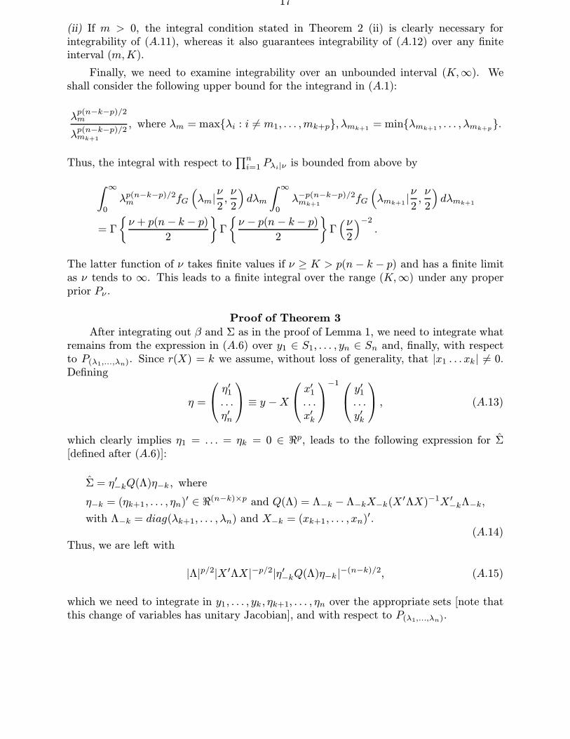
(ii) If m > 0, the integral condition stated in Theorem 2 (ii) is clearly necessary forintegrability of (A.11), whereas it also guarantees integrability of (A.12) over any finiteinterval (m,K).

Finally, we need to examine integrability over an unbounded interval (K,∞). Weshall consider the following upper bound for the integrand in (A.1):

λp(n−k−p)/2m

λp(n−k−p)/2mk+1

, where λm = maxλi : i 6= m1, . . . ,mk+p, λmk+1 = minλmk+1 , . . . , λmk+p.

Thus, the integral with respect to∏ni=1 Pλi|ν is bounded from above by∫ ∞

0

λp(n−k−p)/2m fG

(λm|

ν

2,ν

2

)dλm

∫ ∞0

λ−p(n−k−p)/2mk+1

fG

(λmk+1 |

ν

2,ν

2

)dλmk+1

= Γ

ν + p(n − k − p)

2

Γ

ν − p(n − k − p)

2

Γ(ν

2

)−2

.

The latter function of ν takes finite values if ν ≥ K > p(n − k − p) and has a finite limitas ν tends to ∞. This leads to a finite integral over the range (K,∞) under any properprior Pν .

Proof of Theorem 3After integrating out β and Σ as in the proof of Lemma 1, we need to integrate what

remains from the expression in (A.6) over y1 ∈ S1, . . . , yn ∈ Sn and, finally, with respectto P(λ1,...,λn). Since r(X) = k we assume, without loss of generality, that |x1 . . . xk| 6= 0.Defining

η =

η′1. . .η′n

≡ y −X x′1. . .x′k

−1 y′1. . .y′k

, (A.13)

which clearly implies η1 = . . . = ηk = 0 ∈ <p, leads to the following expression for Σ[defined after (A.6)]:

Σ = η′−kQ(Λ)η−k , where

η−k = (ηk+1, . . . , ηn)′ ∈ <(n−k)×p and Q(Λ) = Λ−k − Λ−kX−k(X ′ΛX)−1X ′−kΛ−k,

with Λ−k = diag(λk+1, . . . , λn) and X−k = (xk+1, . . . , xn)′.(A.14)

Thus, we are left with

|Λ|p/2|X ′ΛX|−p/2|η′−kQ(Λ)η−k|−(n−k)/2, (A.15)

which we need to integrate in y1, . . . , yk , ηk+1, . . . , ηn over the appropriate sets [note thatthis change of variables has unitary Jacobian], and with respect to P(λ1,...,λn).

18

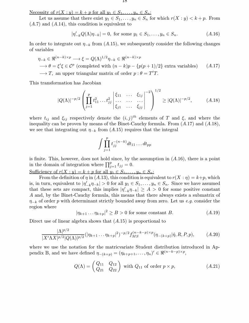
Necessity of r(X : y) = k + p for all y1 ∈ S1, . . . , yn ∈ Sn:Let us assume that there exist y1 ∈ S1, . . . , yn ∈ Sn for which r(X : y) < k+ p. From

(A.7) and (A.14), this condition is equivalent to

|η′−kQ(Λ)η−k| = 0, for some y1 ∈ S1, . . . , yn ∈ Sn. (A.16)

In order to integrate out η−k from (A.15), we subsequently consider the following changesof variables

η−k ∈ <(n−k)×p −→ ξ = Q(Λ)1/2η−k ∈ <

(n−k)×p

−→ θ = ξ′ξ ∈ Cp (completed with (n− k)p− p(p+ 1)/2 extra variables)

−→ T, an upper triangular matrix of order p : θ = T ′T.

(A.17)

This transformation has Jacobian

|Q(Λ)|−p/2

p∏j=1

t211 . . . t2jj

∣∣∣∣∣∣ξ11 . . . ξ1j. . . . . . . . .ξj1 . . . ξjj

∣∣∣∣∣∣−2

1/2

≥ |Q(Λ)|−p/2, (A.18)

where tij and ξij respectively denote the (i, j)th elements of T and ξ, and where theinequality can be proven by means of the Binet-Cauchy formula. From (A.17) and (A.18),we see that integrating out η−k from (A.15) requires that the integral∫ p∏

j=1

t−(n−k)jj dt11 . . . dtpp

is finite. This, however, does not hold since, by the assumption in (A.16), there is a pointin the domain of integration where

∏pj=1 tjj = 0.

Sufficiency of r(X : y) = k + p for all y1 ∈ S1, . . . , yn ∈ Sn:From the definition of η in (A.13), this condition is equivalent to r(X : η) = k+p, which

is, in turn, equivalent to |η′−kη−k| > 0 for all y1 ∈ S1, . . . , yn ∈ Sn. Since we have assumedthat these sets are compact, this implies |η′−kη−k| ≥ A > 0 for some positive constantA and, by the Binet-Cauchy formula, this means that there always exists a submatrix ofη−k of order p with determinant strictly bounded away from zero. Let us e.g. consider theregion where

|ηk+1 . . . ηk+p|2 ≥ B > 0 for some constant B. (A.19)

Direct use of linear algebra shows that (A.15) is proportional to

|Λ|p/2

|X ′ΛX|p/2|Q(Λ)|p/2(|ηk+1 . . . ηk+p|

2)−p/2f(n−k−p)×pMS (η−(k+p)|η, R, P, p), (A.20)

where we use the notation for the matricvariate Student distribution introduced in Ap-pendix B, and we have defined η−(k+p) = (ηk+p+1, . . . , ηn)′ ∈ <(n−k−p)×p,

Q(Λ) =

(Q11 Q12

Q21 Q22

)with Q11 of order p× p, (A.21)

19

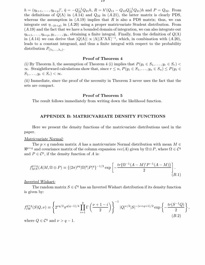
h = (ηk+1, . . . , ηk+p)′, η = −Q−122 Q21h, R = h′(Q11 −Q12Q

−122 Q21)h and P = Q22. From

the definitions of Q(Λ) in (A.14) and Q22 in (A.21), the latter matrix is clearly PDS,whereas the assumption in (A.19) implies that R is also a PDS matrix; thus, we canintegrate out η−(k+p) in (A.20) using a proper matricvariate Student distribution. From(A.19) and the fact that we have a bounded domain of integration, we can also integrate outηk+1, . . . , ηk+p, y1, . . . , yk, obtaining a finite integral. Finally, from the definition of Q(Λ)in (A.14) we can derive that |Q(Λ)| ∝ |Λ||X ′ΛX|−1, which, in combination with (A.20),leads to a constant integrand, and thus a finite integral with respect to the probabilitydistribution P(λ1,...,λn).

Proof of Theorem 4

(i) By Theorem 3, the assumption of Theorem 4 (i) implies that P (y1 ∈ S1, . . . , yr ∈ Sr) <∞. Straightforward calculations show that, since r ≤ n, P (y1 ∈ S1, . . . , yn ∈ Sn) ≤ P (y1 ∈S1, . . . , yr ∈ Sr) <∞.

(ii) Immediate, since the proof of the necessity in Theorem 3 never uses the fact that thesets are compact.

Proof of Theorem 5

The result follows immediately from writing down the likelihood function.

APPENDIX B: MATRICVARIATE DENSITY FUNCTIONS

Here we present the density functions of the matricvariate distributions used in thepaper.

Matricvariate Normal:

The p× q random matrix A has a matricvariate Normal distribution with mean M ∈<p×q and covariance matrix of the column expansion vec(A) given by Ω⊗P , where Ω ∈ Cq

and P ∈ Cp, if the density function of A is:

fp×qMN (A|M,Ω ⊗ P ) ≡ (2π)pq |Ω|p|P |q−1/2 exp

[−trΩ−1(A−M)′P−1(A−M)

2

].

(B.1)

Inverted Wishart:

The random matrix S ∈ Cq has an Inverted Wishart distribution if its density functionis given by:

fq×qIW (S|Q, ν) ≡

2νq/2πq(q−1)/4

q∏i=1

Γ

(ν + 1− i

2

)−1

|Q|ν/2|S|−(ν+q+1)/2 exp

−tr(S−1Q)

2

,

(B.2)where Q ∈ Cq and ν > q − 1.

20

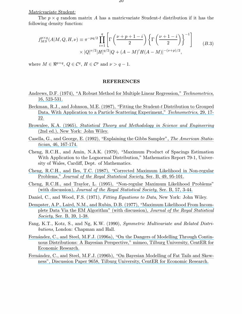
Matricvariate Student:The p × q random matrix A has a matricvariate Student-t distribution if it has the

following density function:

fp×qMS (A|M,Q,H, ν) ≡ π−pq/2q∏i=1

[Γ

(ν + p + 1− i

2

)Γ

(ν + 1− i

2

)−1]

× |Q|ν/2|H|q/2|Q+ (A−M)′H(A−M)|−(ν+p)/2,

(B.3)

where M ∈ <p×q, Q ∈ Cq, H ∈ Cp and ν > q − 1.

REFERENCES

Andrews, D.F. (1974), “A Robust Method for Multiple Linear Regression,” Technometrics,16, 523-531.

Beckman, R.J., and Johnson, M.E. (1987), “Fitting the Student-t Distribution to GroupedData, With Application to a Particle Scattering Experiment,” Technometrics, 29, 17-22.

Brownlee, K.A. (1965), Statistical Theory and Methodology in Science and Engineering(2nd ed.), New York: John Wiley.

Casella, G., and George, E. (1992), “Explaining the Gibbs Sampler”, The American Statis-tician, 46, 167-174.

Cheng, R.C.H., and Amin, N.A.K. (1979), “Maximum Product of Spacings EstimationWith Application to the Lognormal Distribution,” Mathematics Report 79-1, Univer-sity of Wales, Cardiff, Dept. of Mathematics.

Cheng, R.C.H., and Iles, T.C. (1987), “Corrected Maximum Likelihood in Non-regularProblems,” Journal of the Royal Statistical Society, Ser. B, 49, 95-101.

Cheng, R.C.H., and Traylor, L. (1995), “Non-regular Maximum Likelihood Problems”(with discussion), Journal of the Royal Statistical Society, Ser. B, 57, 3-44.

Daniel, C., and Wood, F.S. (1971), Fitting Equations to Data, New York: John Wiley.

Dempster, A.P., Laird, N.M., and Rubin, D.B. (1977), “Maximum Likelihood From Incom-plete Data Via the EM Algorithm” (with discussion), Journal of the Royal StatisticalSociety, Ser. B, 39, 1-38.

Fang, K.T., Kotz, S., and Ng, K.W. (1990), Symmetric Multivariate and Related Distri-butions, London: Chapman and Hall.

Fernandez, C., and Steel, M.F.J. (1996a), “On the Dangers of Modelling Through Contin-uous Distributions: A Bayesian Perspective,” mimeo, Tilburg University, CentER forEconomic Research.

Fernandez, C., and Steel, M.F.J. (1996b), “On Bayesian Modelling of Fat Tails and Skew-ness”, Discussion Paper 9658, Tilburg University, CentER for Economic Research.

21

Fisher, F.A. (1936), “The Use of Multiple Measurements in Taxonomic Problems,” Annalsof Eugenics, 8, 179-188.

Gantmacher, F.R. (1959), The Theory of Matrices (Vol.1), New York: Chelsea.

Gelfand, A., and Smith, A.F.M. (1990), “Sampling-Based Approaches to CalculatingMarginal Densities”, Journal of the American Statistal Association, 85, 398-409.

Geweke, J. (1993), “Bayesian Treatment of the Independent Student-t Linear Model,”Journal of Applied Econometrics, 8, S19-S40.

Geweke, J. (1994), “Priors for Macroeconomic Time Series and Their Applications,” Econo-metric Theory, 10, 609-632.

Giesbrecht, F., and Kempthorne, O. (1976), “Maximum Likelihood Estimation in theThree-parameter Lognormal Distribution”, Journal of the Royal Statistical Society,Ser. B, 38, 257-264.

Gnanadesikan, R. (1977), Methods for Statistical Data Analysis of Multivariate Observa-tions, New York: John Wiley.

Heitjan, D.F. (1989), “Inference From Grouped Continuous Data: A Review” (with dis-cussion), Statistical Science, 4, 164-183.

Kong, A., Liu, J.S., and Wong, W.H. (1994), “Sequential Imputations and Bayesian Miss-ing Data Problems,” Journal of the American Statistical Association, 89, 278-288.

Lange, K.L., Little, R.J.A., and Taylor, J.M.G. (1989), “Robust Statistical Modeling Usingthe t-Distribution. Journal of the American Statistical Association, 84, 881-896.

Lange, K.L., and Sinsheimer, J.S. (1993), “Normal/Independent Distributions and TheirApplications in Robust Regression,” Journal of Computational and Graphical Statis-tics, 2, 175-198.

Lehmann, E.L. (1983), Theory of Point Estimation, New York: John Wiley.

Liu, C.H. (1995), “Missing Data Imputation Using the Multivariate t Distribution,” Jour-nal of Multivariate Analysis, 53, 139-158.

Liu, C.H. (1996), “Bayesian Robust Multivariate Linear Regression With IncompleteData,” Journal of the American Statistical Association, 91, 1219-1227.

Liu, C.H., and Rubin, D.B. (1994), “The ECME Algorithm: A Simple Extension of EMand ECM With Faster Monotone Convergence,” Biometrika, 81, 633-648.

Liu, C.H., and Rubin, D.B. (1995), “ML Estimation of the Multivariate t DistributionWith Unknown Degrees of Freedom,” Statistica Sinica, 5, 19-39.

Maronna, R. (1976), “Robust M-estimators of Multivariate Location and Scatter,” Annalsof Statistics, 4, 51-67.

Murray, G.D. (1977), Comment on “Maximum Likelihood From Incomplete Data Via theEM Algorithm,” by A.P. Dempster, N.M.Laird, and D.B. Rubin, Journal of the RoyalStatistical Society, Ser. B, 39, 27-28.

Pettitt, A.N. (1985), “Re-Weighted Least Squares Estimation With Censored and GroupedData: An Application of the EM Algorithm,” Journal of the Royal Statistical Society,Ser. B, 47, 253-260.

22

Relles, D.A., and Rogers, W.H. (1977), “Statisticians Are Fairly Robust Estimators ofLocation,” Journal of the American Statistical Association, 72, 107-111.

Resek, R.W. (1976), “Estimation of the Parameters of a General Student’s t Distribution,”Communications in Statistics, Part A-Theory and Methods, 5, 635-645.

Rousseeuw, P.J., and van Zomeren, B.C. (1990), “Unmasking Multivariate Outliers andLeverage Points,” Journal of the American Statistical Association, 85, 633-639.

Rubin, D.B. (1987), “A Noniterative Sampling/Importance Resampling Alternative to theData Augmentation Algorithm for Creating a Few Imputations When Fractions ofMissing Observations Are Modest: The SIR Algorithm, Comment on Tanner andWong (1987),” Journal of the American Statistical Association, 82, 543-546.

Smith, R.L. (1989), “A Survey of Nonregular Problems,” in Proceedings of the InternationalStatistical Institute Conference, 47th Session, pp.353-372.

Tanner, M.A., and Wong, W.H. (1987), “The Calculation of Posterior Distributions byData Augmentation” (with discussion), Journal of the American Statistical Associa-tion, 82, 528-550.

Tiede, J.J., and Pagano, M. (1979), “The Application of Robust Calibration to Radioim-munoassay,” Biometrics, 35, 567-574.

West, M. (1984), “Outlier Models and Prior Distributions in Bayesian Linear Regression,”Journal of the Royal Statistical Society, Ser. B, 46, 431-439.

Zellner, A. (1962), “An Efficient Method of Estimating Seemingly Unrelated Regressionsand Tests for Aggregation Bias,” Journal of the American Statistical Association, 58,977-992.

23

Figure 1(a): Posterior Inference Through Set Observations

-2 -1 1 2

-2

-1.5

-1

-0.5

0.5

1

1.5

Figure 1(b): No Posterior Inference Through Set Observations

-3 -2 -1 1 2 3

-0.5

0.5

1

1.5

24

25

26

Figure 10: Set Observations With Missing Components Do Not Help

-6 -4 -2 2 4 6

-4

-2

2

4

6

Figure 11: Compact Set Observations in Murray Data

-2 -1.5 -1 -0.5 0.5 1 1.5

-1.5

-1

-0.5

0.5

1

1.5

2

27

28