Studying Co-movements in Large Multivariate Data

Prior to Multivariate Modelling�

Gianluca Cubadda

Università di Roma "Tor Vergata"

Alain Hecq

Maastricht University

Franz C. Palmy

Maastricht University

September 23, 2008

Abstract

For non-stationary vector autoregressive models (VAR hereafter, or VAR with moving average,

VARMA hereafter), we show that the presence of common cyclical features or cointegration leads to

a reduction of the order of the implied univariate autoregressive-moving average (ARIMA hereafter)

models. This �nding can explain why we identify parsimonious univariate ARIMA models in applied

research although VAR models of typical order and dimension used in macroeconometrics imply non-

parsimonious univariate ARIMA representations.

Next, we develop a strategy for studying interactions between variables prior to possibly modelling

them in a multivariate setting. Indeed, the similarity of the autoregressive roots will be informative

about the presence of co-movements in a set of multiple time series. Our results justify both the use of a

panel setup with homogeneous autoregression and heterogeneous cross-correlated vector moving average

errors and a factor structure, and the use of cross-sectional aggregates of ARIMA series to estimate the

homogeneous autoregression.

Keywords: Interactions, multiple time series, co-movements, ARIMA, cointegration, common cycles,

dynamic panel data. JEL: C32

�Previous drafts of this paper were presented at the Joint Statistical Meetings in Salt Lake City, 62nd European Meeting ofthe Econometric Society in Budapest, and EC2 Conference on Advanced Time Series Econometrics in Faro. We wish to thanktwo anonymous referees and the editor Arnold Zellner for useful comments. The usual disclaimers apply.

yCorresponding author: Franz C. Palm, Maastricht University, Department of Quantitative Economics, P.O.Box 616, 6200MD Maastricht, The Netherlands. Email: f.palm@ke.unimaas.nl.

1

1 Introduction

The analysis of interactions between individuals, groups of agents, organizations, regions or countries is a

key objective of scienti�c inquiry. Huge collections of data (national accounts for virtually all countries,

unemployment data for hundreds of types of jobs, prices for thousands of products, assets and services,

purchases by individual consumers, environmental data on CO2 emissions and climate change, on health

care, education,. . . ) are almost instantaneously available at relatively low cost. The IMF and the World

Bank publish statistical information for 150 countries. In the European Union, starting for the six founding

countries, Eurostat now collects and analyzes hundreds of variables for the 27 member countries. The

availability of sets of data for a large number of individual entities and the importance of understanding

individual behavior and interaction between individuals have created a demand for methods to analyze these

types of phenomena using large sets of data.

To capture interactions between a large set of time series requires imposing structure on the models used

in the analysis. Examples of structure often imposed are the dynamic factor models put forward by Forni et

al. (2000) and by Stock and Watson (2002). Another example is the approach of using the common factor

structure adopted in the recent literature on dynamic macro-panels to account for cross-sectional correlation

(e.g. Bai and Ng, 2004). In these approaches, the common factors usually account for the impact of changes

in the environment that is largely exogenous and in which individual entities have to take decisions and to

interact. Individual speci�cities are often accounted for by including individual e¤ects.

Alternatively, partial systems are built for country-speci�c analyses or for a speci�c variable such as

for instance GDP for a subset of countries or regions. An often adopted framework to analyze a limited

number of time series is the vector autoregressive model (VAR hereafter). A VAR, allowing all variables

to be endogenous, can only be implemented for small systems, with typically �ve or six variables. Still, in

such cases, the number of parameters is large. To deal with the dimensionality problem in VARs, di¤erent

approaches have been adopted such as inter alia Bayesian analysis, simulation-based techniques, separability

assumptions (as for instance used in panel data models when they are accompanied by the homogeneity

assumption of the autoregressive parameters across units), automatic selection by deleting non-signi�cant

coe¢ cients and reduced-rank regressions.

In this paper we take a di¤erent route and make two new contributions to the literature. Instead of

designing a system which captures interactions between entities, we �rst address the question what the

implications are of the presence of common factors in a possibly large VAR system on the marginal processes

for individual entities. The common factor structure could arise from the presence of common cyclical or

other features (see e.g. Engle and Kozicki, 1993). For non-stationary series, a common factor structure

could result from the presence of cointegration, that is from the occurrence of common stochastic trends.

The �rst main contribution of the paper is that the presence of common factors or common features in a VAR

leads to a reduction of the order of the implied univariate autoregressive-moving average (ARIMA hereafter)

schemes for the individual series. In a way, individual series keep a print of the system as a whole. Second,

we propose a strategy, that allows to identify the print of common features from individual data, that is to

study aspects of interactions between individual variables without or prior to modelling these interactions

2

in a multivariate framework.

Before implementing this strategy, we derive the implications of the presence of a common factor structure

for the univariate processes implied by a VAR, both in absence of and under exogeneity restrictions. More

precisely, in Section 2, we extend results by Zellner and Palm (1974) by showing that VARs with reduced

rank restrictions coming from short- or long-run co-movements (see inter alia Vahid and Engle, 1993, and

Ahn, 1997) o¤er an alternative explanation to the well known paradox in time series: on the one hand,

small multivariate systems imply non-parsimonious individual ARIMA processes whereas on the other hand

empirically selected and estimated univariate models are generally of low order.

Section 3 proposes and evaluates an estimation strategy based upon the common univariate autoregressive

parameters of series generated by the same VAR system. Indeed, a homogeneous panel framework with

common autoregressive parameters is the by-product of a large VAR. We propose to use cross-sectional

aggregates to estimate these common autoregressive parameters, and we evaluate this estimation strategy

in a small Monte Carlo experiment. Section 4 focuses on the link between the growth rates of GDP among

Latin American economies. The occurrence of common autoregressive parts for the individual series is used

as an indication that these series exhibit the same common features and therefore are subject to the same

co-movements. This indication is then formally tested and found to be supported by the information in the

data. A �nal section concludes and provides suggestions for further research.

2 Multivariate and implied univariate time series models

The aim of this section is to present new results on the relations between univariate and multivariate time

series models. In particular, Subsection 2.1 brie�y reviews the paradox, namely that VARs of typical order

and dimension used in macroeconometrics imply non-parsimonious univariate ARMA representations, which

are rarely observed in empirical applications. Subsection 2.2 shows how VARs with certain reduced rank

structures can solve this paradox, and Subsection 2.3 specializes the results to the case of block-diagonal

and block-triangular VARs. Moreover, Subsection 2.4 explores the implications of short-run co-movements

for the vector moving average (VMA hereafter) component of the so-called �nal equation representation of

a VAR model (Zellner and Palm, 1974). The �ndings may explain why MA orders of univariate models are

often found to be smaller than those theoretically implied by multivariate models. Finally, Subsection 2.5

illustrates concepts and methods with an empirical analysis of the relationship between quarterly growth

rates of the industrial production indexes in the US and Canada.

2.1 The paradox

The literature on the link between multivariate time series and the behavior of univariate variables stresses

the fact that univariate ARIMA analyses provide tools for the diagnostic testing of VAR (or VARMA)

models. Important contributions in this area are the monograph by Quenouille (1957) and papers by Zellner

and Palm (1974, 1975, 2004), Palm and Zellner (1980), Palm (1977) or Maravall and Mathis (1994). Some

textbooks devote a few pages to that issue (e.g. Franses (1998, 198-199) or Lütkepohl (2005, 494-495)).

3

More formally, let us �rst consider the stationary1 multivariate VARMA process for an n vector of time

series zt = (z1t; : : : ; znt)0, and without deterministic terms for simplicity:

�(L)zt = �(L)"t; t = 1; : : : ; T; (1)

where �(L) and �(L) are �nite order polynomial coe¢ cient matrices with the usual lag operator L such that

Lzt = zt�1: The sequence of "t is a multivariate white noise process with each "t � N(0;�): The VARMAmodel in (1) encompasses several useful speci�cations. For example, if �(L) � I we have the vector movingaverage representation or VMA; if �(L) � I we have a VAR(p). Let us concentrate the analysis on VAR

models of order p, denoted VAR(p), one of the cornerstone speci�cation in empirical macroeconometrics:

�(L)zt = "t: (2)

Following Zellner and Palm (1974), the univariate representation of elements of zt can be obtained by

premultiplying both sides of (2) by �(L)adj ; the adjoint matrix (or the adjugate) associated with �(L); in

order to obtain the "�nal equations" (FEs henceforth):

det[�(L)]zt = �(L)adj"t; (3)

where the determinant det[�(L)] is a scalar �nite order polynomial in L: This means that each series is a

�nite order ARMA(p�; q�), with the same lag structure and the same coe¢ cients for the autoregressive part

for every series, although the multivariate system is a �nite order VAR(p). For instance for the ith element

of zt we have

det[�(L)]zit = �i�(L)adj"t = �i(L)uit;

�i�(L)adj denoting the ith row of the matrix �(L)adj ; �i(L) is a scalar polynomial in L and uit is a scalar

innovation with respect to the past of zit: This recognition and the compatibility of these p� and q� with n

and p of the VAR(p) is the �rst step of an approach that has been developed in Zellner and Palm (1974, 1975)

as a general modelling strategy called SEMTSA (Structural Economic Modelling Time Series Analysis). In

the �rst stage of this approach, information from univariate schemes is used to restrict the dynamics of the

structural model. However, given the conditions associated with that �rst diagnostic checking, one often

faces a paradoxical situation: a small order VAR with few series already generates univariate ARMA with

large p� and q�, an implication that is rejected when tested on economic data where one usually �nds quite

parsimonious models with low order autoregressive and moving average polynomials.

Indeed, an n dimensional VAR(p) would imply at most individual ARMA(np; (n� 1)p) processes. Thiswell known result is simply due to the fact that det[�(L)] contains by construction up to Lnp terms and the

adjoint matrix is a collection (n � 1) � (n � 1) cofactor matrices, each of the matrix elements can containthe terms 1; L; ::Lp: But whatever the simplicity of that result, it leads to implausible univariate models for

1The generalisation to non-stationarity processes will be considered later in this section..

4

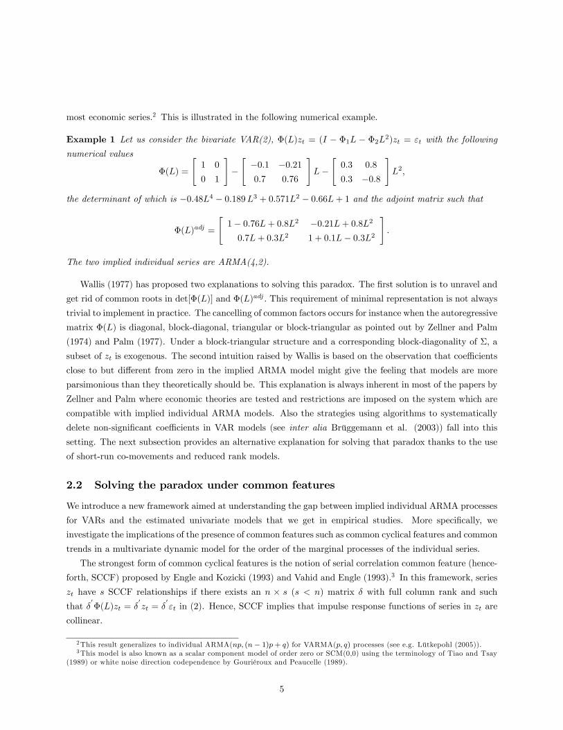
most economic series.2 This is illustrated in the following numerical example.

Example 1 Let us consider the bivariate VAR(2), �(L)zt = (I � �1L � �2L2)zt = "t with the following

numerical values

�(L) =

"1 0

0 1

#�"�0:1 �0:210:7 0:76

#L�

"0:3 0:8

0:3 �0:8

#L2;

the determinant of which is �0:48L4 � 0:189L3 + 0:571L2 � 0:66L+ 1 and the adjoint matrix such that

�(L)adj =

"1� 0:76L+ 0:8L2 �0:21L+ 0:8L2

0:7L+ 0:3L2 1 + 0:1L� 0:3L2

#:

The two implied individual series are ARMA(4,2).

Wallis (1977) has proposed two explanations to solving this paradox. The �rst solution is to unravel and

get rid of common roots in det[�(L)] and �(L)adj : This requirement of minimal representation is not always

trivial to implement in practice. The cancelling of common factors occurs for instance when the autoregressive

matrix �(L) is diagonal, block-diagonal, triangular or block-triangular as pointed out by Zellner and Palm

(1974) and Palm (1977). Under a block-triangular structure and a corresponding block-diagonality of �; a

subset of zt is exogenous. The second intuition raised by Wallis is based on the observation that coe¢ cients

close to but di¤erent from zero in the implied ARMA model might give the feeling that models are more

parsimonious than they theoretically should be. This explanation is always inherent in most of the papers by

Zellner and Palm where economic theories are tested and restrictions are imposed on the system which are

compatible with implied individual ARMA models. Also the strategies using algorithms to systematically

delete non-signi�cant coe¢ cients in VAR models (see inter alia Brüggemann et al. (2003)) fall into this

setting. The next subsection provides an alternative explanation for solving that paradox thanks to the use

of short-run co-movements and reduced rank models.

2.2 Solving the paradox under common features

We introduce a new framework aimed at understanding the gap between implied individual ARMA processes

for VARs and the estimated univariate models that we get in empirical studies. More speci�cally, we

investigate the implications of the presence of common features such as common cyclical features and common

trends in a multivariate dynamic model for the order of the marginal processes of the individual series.

The strongest form of common cyclical features is the notion of serial correlation common feature (hence-

forth, SCCF) proposed by Engle and Kozicki (1993) and Vahid and Engle (1993).3 In this framework, series

zt have s SCCF relationships if there exists an n � s (s < n) matrix � with full column rank and such

that �0�(L)zt = �

0zt = �

0"t in (2). Hence, SCCF implies that impulse response functions of series in zt are

collinear.

2This result generalizes to individual ARMA(np; (n� 1)p+ q) for VARMA(p; q) processes (see e.g. Lütkepohl (2005)).3This model is also known as a scalar component model of order zero or SCM(0,0) using the terminology of Tiao and Tsay

(1989) or white noise direction codependence by Gouriéroux and Peaucelle (1989).

5

Although convenient in terms of parsimony and economic interpretation of shocks�transmission mecha-

nisms (see, inter alia, Centoni et al., 2007), assumptions underlying SCCF may be too strong. Indeed, the

de�nition of SCCF does not take account of the possibility that common serial correlation is present among

non-contemporaneous elements of series zt (see e.g. Ericsson, 1993). In order to overcome this limitation,

several variants of the SCCF were proposed, see, inter alia, Vahid and Engle (1997), Schleicher (2007), Hecq

et al. (2006), Cubadda (2007), and Cubadda and Hecq (2001). In particular, these latter authors assume

that there exists an n � s polynomial matrix such that �0(L)zt � (�0 + �1L)0zt = �

0

0"t. This model is a

polynomial SCCF model of order one, which is denoted PSCCF(1).4 The notion of PSCCF can be general-

ized to account for adjustment delays of m periods instead of one lag as in the PSCCF(1). In this case the

polynomial matrix �(L) is of order m, where m � p, a model denoted PSCCF(m) (see Cubadda and Hecq(2001) for details).

For simplicity reasons, we start with the most parsimonious model, in which there exists a SCCF matrix.

We �rst illustrate the consequences of the presence of one SCCF relationship in a bivariate example with

p = 2 before generalizing to the n dimensional case for any polynomial order p and other forms of non

contemporaneous co-movements (e.g. PSCCF):

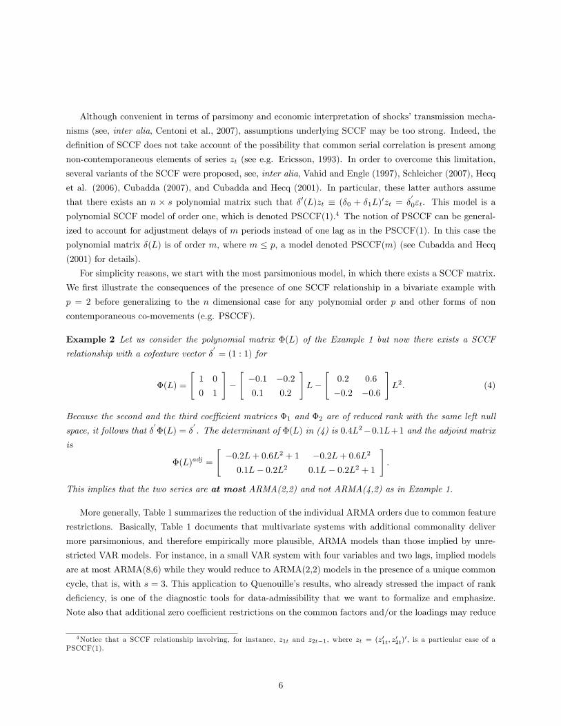
Example 2 Let us consider the polynomial matrix �(L) of the Example 1 but now there exists a SCCF

relationship with a cofeature vector �0= (1 : 1) for

�(L) =

"1 0

0 1

#�"�0:1 �0:20:1 0:2

#L�

"0:2 0:6

�0:2 �0:6

#L2: (4)

Because the second and the third coe¢ cient matrices �1 and �2 are of reduced rank with the same left null

space, it follows that �0�(L) = �

0. The determinant of �(L) in (4) is 0:4L2�0:1L+1 and the adjoint matrix

is

�(L)adj =

"�0:2L+ 0:6L2 + 1 �0:2L+ 0:6L2

0:1L� 0:2L2 0:1L� 0:2L2 + 1

#:

This implies that the two series are at most ARMA(2,2) and not ARMA(4,2) as in Example 1.

More generally, Table 1 summarizes the reduction of the individual ARMA orders due to common feature

restrictions. Basically, Table 1 documents that multivariate systems with additional commonality deliver

more parsimonious, and therefore empirically more plausible, ARMA models than those implied by unre-

stricted VAR models. For instance, in a small VAR system with four variables and two lags, implied models

are at most ARMA(8,6) while they would reduce to ARMA(2,2) models in the presence of a unique common

cycle, that is, with s = 3: This application to Quenouille�s results, who already stressed the impact of rank

de�ciency, is one of the diagnostic tools for data-admissibility that we want to formalize and emphasize.

Note also that additional zero coe¢ cient restrictions on the common factors and/or the loadings may reduce

4Notice that a SCCF relationship involving, for instance, z1t and z2t�1, where zt = (z01t; z02t)

0, is a particular case of aPSCCF(1).

6

these implied maximal orders. This means that the ARMA(2,2) obtained under short-run co-movements can

be more parsimonious with additional exclusion restrictions.

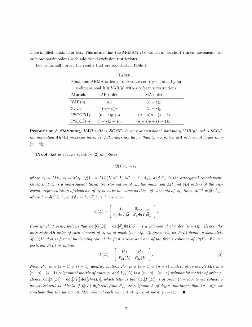
Let us formally prove the results that are reported in Table 1.

Table 1

Maximum ARMA orders of univariate series generated by an

n-dimensional I(0) VAR(p) with s cofeature restrictions

Models AR order MA order

VAR(p) np (n� 1)pSCCF (n� s)p (n� s)pPSCCF(1) (n� s)p+ s (n� s)p+ (s� 1)PSCCF(m) (n� s)p+ sm (n� s)p+ (s� 1)m

Proposition 3 Stationary VAR with s SCCF. In an n-dimensional stationary VAR(p) with s SCCF,

the individual ARMA processes have: (i) AR orders not larger than (n� s)p; (ii) MA orders not larger than(n� s)p.

Proof. Let us rewrite equation (2) as follows

Q(L)xt = et;

where xt = Mzt, et = M"t, Q(L) = M�(L)M�1, M 0 � [� : �?], and �? is the orthogonal complement.

Given that xt is a non-singular linear transformation of zt, the maximum AR and MA orders of the uni-

variate representation of elements of zt must be the same as those of elements of xt. Since M�1 = [� : �?],

where � = �(�0�)�1, and �? = �?(�0?�?)

�1, we have

Q(L) =

"Is 0s�(n�s)

�0?�(L)� �0?�(L)�?

#;

from which it easily follows that det[Q(L)] = det[�0?�(L)�?] is a polynomial of order (n � s)p. Hence, theunivariate AR order of each element of zt is, at most, (n� s)p. To prove (ii), let P (L) denote a submatrixof Q(L) that is formed by deleting one of the �rst s rows and one of the �rst s columns of Q(L). We can

partition P (L) as follows

P (L) =

"P11 P12

P21(L) P22(L)

#: (5)

Now, P11 is a (s � 1) � (s � 1) identity matrix, P12 is a (s � 1) � (n � s) matrix of zeros, P21(L) is a(n�s)� (s�1) polynomial matrix of order p, and P22(L) is a (n�s)� (n�s) polynomial matrix of order p.Hence, det[P (L)] = det[P11] det[P22(L)], which tells us that det[P (L)] is of order (n� s)p. Since cofactorsassociated with the blocks of Q(L) di¤erent from P11 are polynomials of degree not larger than (n� s)p, weconclude that the univariate MA order of each element of zt is, at most, (n� s)p.

7

Proposition 4 Stationary VAR with s PSCCF(1). In an n stationary VAR(p) with s PSCCF(1) the

individual ARMA processes have: (i) AR orders not larger than (n� s)p+ s;(ii) MA orders not larger than(n� s)p+ (s� 1).

Proof. Along the same lines of the previous proof, let us consider R(L) =M0�(L)M�10 ,M 0

0 � [�0 : �0?],and M�1

0 � [�0 : �0?]. Then, we have

R(L) =

"�0(L)�0 �01�0?L

�00?�(L)�0 �00?�(L)�0?

#:

Hence,

det[R(L)] = det[�0(L)�0] det[�00?�(L)�0? � �00?�(L)�0(�0(L)�0)�1�01�0?L]:

Writing (�0(L)�0)�1 = (�0(L)�0)

adj=det[�0(L)�0] and substituting it above we get

det[R(L)]det[�0(L)�0]n�s�1| {z }

s(n�s�1)

= det

8><>:�00?�(L)�0?| {z }p

det[�0(L)�0]| {z }s

� �00?�(L)�0| {z }p

(�0(L)�0)adj| {z }

s�1

�01�0?L| {z }1

9>=>;from which follows that the degree of the polynomial of det[R(L)] is, at most, equal to (n�s)p+s. Regardingthe order of the MA component, let us denote G(L) a submatrix of R(L) that is formed by deleting one of

the �rst s rows and one of the �rst s columns of R(L). We can partition G(L) as follows

G(L) =

"G11(L) G12L

G21(L) G22(L)

#;

where G11(L) is a (s� 1)� (s� 1) polynomial matrix of order 1, G12 is a (s� 1)� (n� s) matrix, G21(L)is a (n � s) � (s � 1) polynomial matrix of order p, and G22(L) is a (n � s) � (n � s) polynomial matrixof order p. Hence, following a similar reasoning as above, we conclude that the individual MA order is, at

most, (n� s)p+ (s� 1).These results can be easily generalized for the PSCCF(m) case as reported in Table 1. Also note that

we do not consider a mixed model that can have both SCCF and PSCCF relationships but results can be

trivially deduced from results beneath.

The above propositions can be extended to the case of an I(1) VAR. Let us consider the vector error

correction model (VECM henceforth) of variables zt

�(L)�zt = ��0zt�1 + "t; (6)

where � = (1 � L), �(L) = In �Pp�1

i=1 �iLi, �i = �

Ppj=i+1 �j for i = 1; 2; :::; p � 1, � and � are full-

column rank n� r (r < n) matrices such that �(1) = ���0 and �0?�(1)�? has full rank. The process zt iscointegrated of order (1,1), denoted by CI(1,1), the columns of � span the cointegrating space, the elements

of � are the corresponding adjustment coe¢ cients, see e.g. Johansen (1996).

8

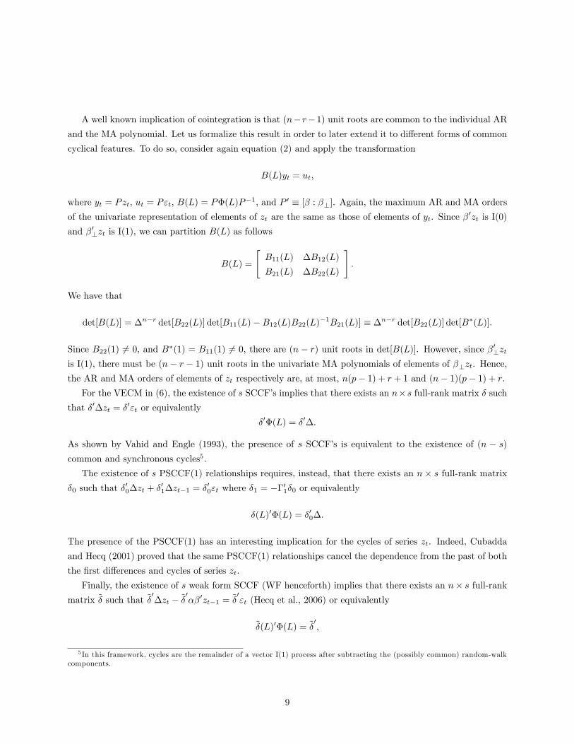
A well known implication of cointegration is that (n� r�1) unit roots are common to the individual ARand the MA polynomial. Let us formalize this result in order to later extend it to di¤erent forms of common

cyclical features. To do so, consider again equation (2) and apply the transformation

B(L)yt = ut;

where yt = Pzt, ut = P"t, B(L) = P�(L)P�1, and P 0 � [� : �?]. Again, the maximum AR and MA orders

of the univariate representation of elements of zt are the same as those of elements of yt. Since �0zt is I(0)

and �0?zt is I(1), we can partition B(L) as follows

B(L) =

"B11(L) �B12(L)

B21(L) �B22(L)

#:

We have that

det[B(L)] = �n�r det[B22(L)] det[B11(L)�B12(L)B22(L)�1B21(L)] � �n�r det[B22(L)] det[B�(L)]:

Since B22(1) 6= 0, and B�(1) = B11(1) 6= 0, there are (n � r) unit roots in det[B(L)]. However, since �0?ztis I(1), there must be (n� r � 1) unit roots in the univariate MA polynomials of elements of �?zt. Hence,the AR and MA orders of elements of zt respectively are, at most, n(p� 1) + r + 1 and (n� 1)(p� 1) + r.For the VECM in (6), the existence of s SCCF�s implies that there exists an n�s full-rank matrix � such

that �0�zt = �0"t or equivalently

�0�(L) = �0�:

As shown by Vahid and Engle (1993), the presence of s SCCF�s is equivalent to the existence of (n � s)common and synchronous cycles5 .

The existence of s PSCCF(1) relationships requires, instead, that there exists an n� s full-rank matrix�0 such that �

00�zt + �

01�zt�1 = �

00"t where �1 = ��01�0 or equivalently

�(L)0�(L) = �00�:

The presence of the PSCCF(1) has an interesting implication for the cycles of series zt. Indeed, Cubadda

and Hecq (2001) proved that the same PSCCF(1) relationships cancel the dependence from the past of both

the �rst di¤erences and cycles of series zt.

Finally, the existence of s weak form SCCF (WF henceforth) implies that there exists an n� s full-rankmatrix ~� such that ~�

0�zt � ~�

0��0zt�1 = ~�

0"t (Hecq et al., 2006) or equivalently

~�(L)0�(L) = ~�0;

5 In this framework, cycles are the remainder of a vector I(1) process after subtracting the (possibly common) random-walkcomponents.

9

where ~�(L) = ~� + ~�1L; ~�1 = �(��0 + In)~�. Interestingly, the same WF relationships cancel the dependencefrom the past of both the levels and cycles of series zt (Cubadda, 2007). Hence, we can interpret the WF as

an analogous property to the PSCCF(1) that applies to the levels rather than to the di¤erences of series zt.

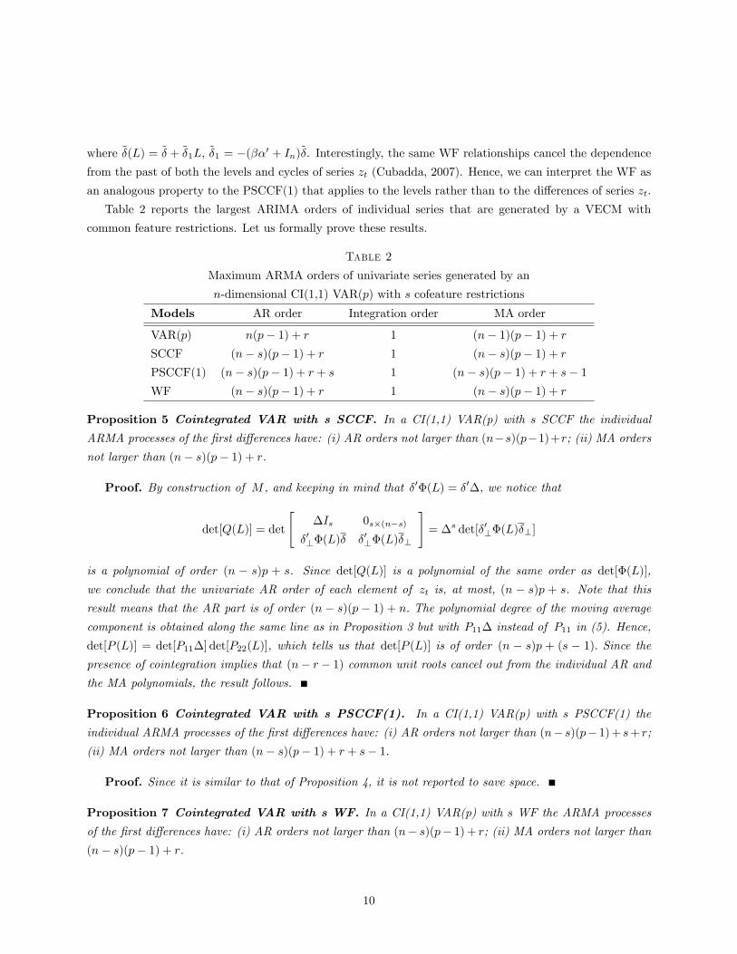
Table 2 reports the largest ARIMA orders of individual series that are generated by a VECM with

common feature restrictions. Let us formally prove these results.

Table 2

Maximum ARMA orders of univariate series generated by an

n-dimensional CI(1,1) VAR(p) with s cofeature restrictions

Models AR order Integration order MA order

VAR(p) n(p� 1) + r 1 (n� 1)(p� 1) + rSCCF (n� s)(p� 1) + r 1 (n� s)(p� 1) + rPSCCF(1) (n� s)(p� 1) + r + s 1 (n� s)(p� 1) + r + s� 1WF (n� s)(p� 1) + r 1 (n� s)(p� 1) + r

Proposition 5 Cointegrated VAR with s SCCF. In a CI(1,1) VAR(p) with s SCCF the individual

ARMA processes of the �rst di¤erences have: (i) AR orders not larger than (n�s)(p�1)+r; (ii) MA ordersnot larger than (n� s)(p� 1) + r.

Proof. By construction of M , and keeping in mind that �0�(L) = �0�, we notice that

det[Q(L)] = det

"�Is 0s�(n�s)

�0?�(L)� �0?�(L)�?

#= �s det[�0?�(L)�?]

is a polynomial of order (n � s)p + s. Since det[Q(L)] is a polynomial of the same order as det[�(L)],we conclude that the univariate AR order of each element of zt is, at most, (n � s)p + s. Note that thisresult means that the AR part is of order (n � s)(p � 1) + n: The polynomial degree of the moving averagecomponent is obtained along the same line as in Proposition 3 but with P11� instead of P11 in (5). Hence,

det[P (L)] = det[P11�] det[P22(L)], which tells us that det[P (L)] is of order (n � s)p + (s � 1): Since thepresence of cointegration implies that (n� r � 1) common unit roots cancel out from the individual AR and

the MA polynomials, the result follows.

Proposition 6 Cointegrated VAR with s PSCCF(1). In a CI(1,1) VAR(p) with s PSCCF(1) the

individual ARMA processes of the �rst di¤erences have: (i) AR orders not larger than (n� s)(p� 1)+ s+ r;(ii) MA orders not larger than (n� s)(p� 1) + r + s� 1.

Proof. Since it is similar to that of Proposition 4, it is not reported to save space.

Proposition 7 Cointegrated VAR with s WF. In a CI(1,1) VAR(p) with s WF the ARMA processes

of the �rst di¤erences have: (i) AR orders not larger than (n� s)(p� 1)+ r; (ii) MA orders not larger than(n� s)(p� 1) + r.

10

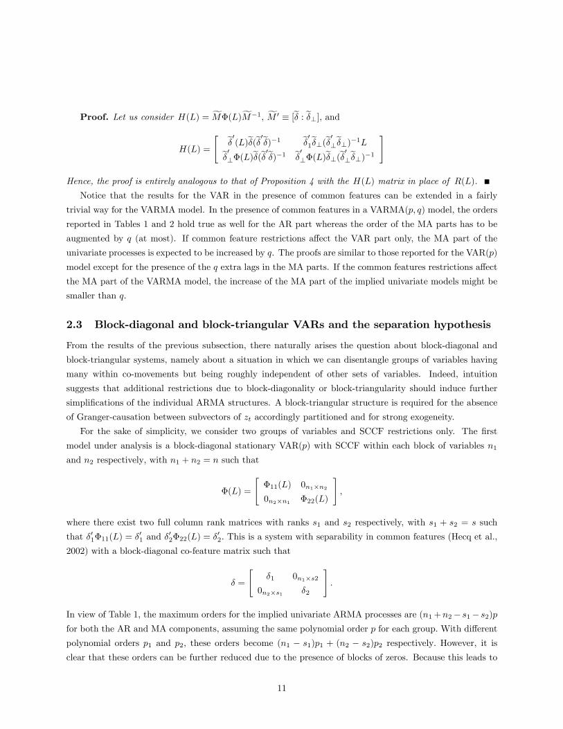
Proof. Let us consider H(L) = fM�(L)fM�1, fM 0 � [e� : e�?], andH(L) =

" e�0(L)e�(e�0e�)�1 e�01e�?(e�0?e�?)�1Le�0?�(L)e�(e�0e�)�1 e�0?�(L)e�?(e�0?e�?)�1#

Hence, the proof is entirely analogous to that of Proposition 4 with the H(L) matrix in place of R(L).

Notice that the results for the VAR in the presence of common features can be extended in a fairly

trivial way for the VARMA model. In the presence of common features in a VARMA(p; q) model, the orders

reported in Tables 1 and 2 hold true as well for the AR part whereas the order of the MA parts has to be

augmented by q (at most). If common feature restrictions a¤ect the VAR part only, the MA part of the

univariate processes is expected to be increased by q. The proofs are similar to those reported for the VAR(p)

model except for the presence of the q extra lags in the MA parts. If the common features restrictions a¤ect

the MA part of the VARMA model, the increase of the MA part of the implied univariate models might be

smaller than q.

2.3 Block-diagonal and block-triangular VARs and the separation hypothesis

From the results of the previous subsection, there naturally arises the question about block-diagonal and

block-triangular systems, namely about a situation in which we can disentangle groups of variables having

many within co-movements but being roughly independent of other sets of variables. Indeed, intuition

suggests that additional restrictions due to block-diagonality or block-triangularity should induce further

simpli�cations of the individual ARMA structures. A block-triangular structure is required for the absence

of Granger-causation between subvectors of zt accordingly partitioned and for strong exogeneity.

For the sake of simplicity, we consider two groups of variables and SCCF restrictions only. The �rst

model under analysis is a block-diagonal stationary VAR(p) with SCCF within each block of variables n1and n2 respectively; with n1 + n2 = n such that

�(L) =

"�11(L) 0n1�n2

0n2�n1 �22(L)

#;

where there exist two full column rank matrices with ranks s1 and s2 respectively, with s1 + s2 = s such

that �01�11(L) = �01 and �

02�22(L) = �

02: This is a system with separability in common features (Hecq et al.,

2002) with a block-diagonal co-feature matrix such that

� =

"�1 0n1�s2

0n2�s1 �2

#:

In view of Table 1, the maximum orders for the implied univariate ARMA processes are (n1+n2� s1� s2)pfor both the AR and MA components, assuming the same polynomial order p for each group:With di¤erent

polynomial orders p1 and p2; these orders become (n1 � s1)p1 + (n2 � s2)p2 respectively: However, it isclear that these orders can be further reduced due to the presence of blocks of zeros. Because this leads to

11

the presence of common roots between the AR and MA parts, the maximum orders of both AR and MA

components are (n1 � s1)p1 for the �rst block and (n2 � s2)p2 for the second group of series.Due to separation in the form of block-diagonality of �(L); the implied univariate ARMA-processes need

not to have identical AR polynomials. In fact, the model allows for inter-block AR parameter heterogeneity

and intra-block AR parameter homogeneity. Note that this form of separation is often used when studying

data for a set of countries using a panel-data framework. In some panel-data studies, a single variable is

analyzed for a set of countries which can be clustered in groups with intergroup block-diagonality of �(L)

combined with intragroup homogeneity so that the implied univariate ARMA models for a given group have

identical AR polynomials.

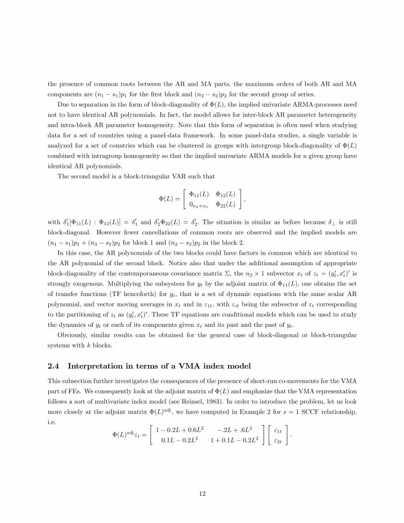
The second model is a block-triangular VAR such that

�(L) =

"�11(L) �12(L)

0n2�n1 �22(L)

#;

with �01[�11(L) : �12(L)] = �01 and �02�22(L) = �02: The situation is similar as before because �? is still

block-diagonal. However fewer cancellations of common roots are observed and the implied models are

(n1 � s1)p1 + (n2 � s2)p2 for block 1 and (n2 � s2)p2 in the block 2.In this case, the AR polynomials of the two blocks could have factors in common which are identical to

the AR polynomial of the second block. Notice also that under the additional assumption of appropriate

block-diagonality of the contemporaneous covariance matrix �; the n2 � 1 subvector xt of zt = (y0t; x0t)0 is

strongly exogenous. Multiplying the subsystem for yt by the adjoint matrix of �11(L); one obtains the set

of transfer functions (TF henceforth) for yt; that is a set of dynamic equations with the same scalar AR

polynomial, and vector moving averages in xt and in "1t; with "it being the subvector of "t corresponding

to the partitioning of zt as (y0t; x0t)0: These TF equations are conditional models which can be used to study

the dynamics of yt or each of its components given xt and its past and the past of yt.

Obviously, similar results can be obtained for the general case of block-diagonal or block-triangular

systems with k blocks.

2.4 Interpretation in terms of a VMA index model

This subsection further investigates the consequences of the presence of short-run co-movements for the VMA

part of FEs. We consequently look at the adjoint matrix of �(L) and emphasize that the VMA representation

follows a sort of multivariate index model (see Reinsel, 1983). In order to introduce the problem, let us look

more closely at the adjoint matrix �(L)adj ; we have computed in Example 2 for s = 1 SCCF relationship;

i.e.

�(L)adj"t =

"1� 0:2L+ 0:6L2 �:2L+ :6L2

0:1L� 0:2L2 1 + 0:1L� 0:2L2

#""1t

"2t

#:

12

We can also write the previous expression in terms of coe¢ cient matrices and we observe the presence of a

common right factor, namely of common right null spaces such that

�(L)adj"t =

""1t

"2t

#+

"�:20:1

# h1 1

i " "1t�1"2t�1

#+

"0:6

�0:2

# h1 1

i " "1t�2"2t�2

#

with the obvious numerical observation that �(L)adj�? = �?, and �0? = (1 : �1). We now show that the

VMA component of (3) has a structure that is analogous to the multivariate index model of Reinsel (1983),

and this leads to the following general proposition:

Proposition 8 In a stationary VAR(p), the existence of s SCCF vectors implies that in the FE represen-

tation the VMA coe¢ cient matrices associated with degrees strictly larger than (n� s� 1)p have a commonright null space that is spanned by �?: Hence, post-multiplying the adjoint matrix �(L)adj by �? reduces the

order of the VMA component to a degree of at most (n� s� 1)p instead of (n� s)p.

Proof. We know from Proposition 3 that det[�(L)] and �(L)adj are both polynomials of order (n� s)p.Moreover, under SCCF we have that

�(L) = In �pXj=1

�?0jL

j ;

where �j = �?0j : Hence we can write

det[�(L)]In = �(L)adj�(L) = �(L)adj � [�(L)adj�?]

pXj=1

0jLj ;

from which it follows that �(L)adj�? is a polynomial of order (n� s� 1)p.

Corollary 9 In the particular case with n� 1 = s, the VMA component of the FEs follows an index modelas in Reinsel (1983).

The last result is more a mathematical curiosity than a device to be used in an empirical analysis. We

might think to use it for fully e¢ cient estimation of the FEs for instance. But this shows that there exists a

factor structure in the VMA component. In empirical investigations, this result can partially explain why the

MA order is often found to be smaller than what it should be according to the theoretical implied models

in Tables 1 and 2. Consider, for instance, the case with wt = "t + H1"t�1, where wt = �(L)adj"t. The

�rst autocovariance of wt = det[�(L)]zt is then given by E(wt�1w0t) = H1� and, since �? spans the right

null space of H1, we have E(wt�1w0t) = 0 when � = �?��0?, where � is a symmetric semi-positive de�nite

matrix. Of course, under the condition � = �?��0? the VAR innovations would be perfectly collinear and

this cannot occur in practice. However, it might well be that � � �?��0?, and we label this case as a nearcoincidental situation.

13

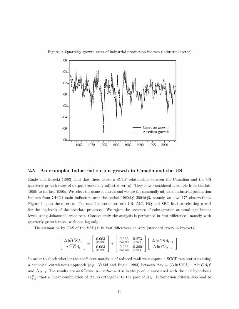
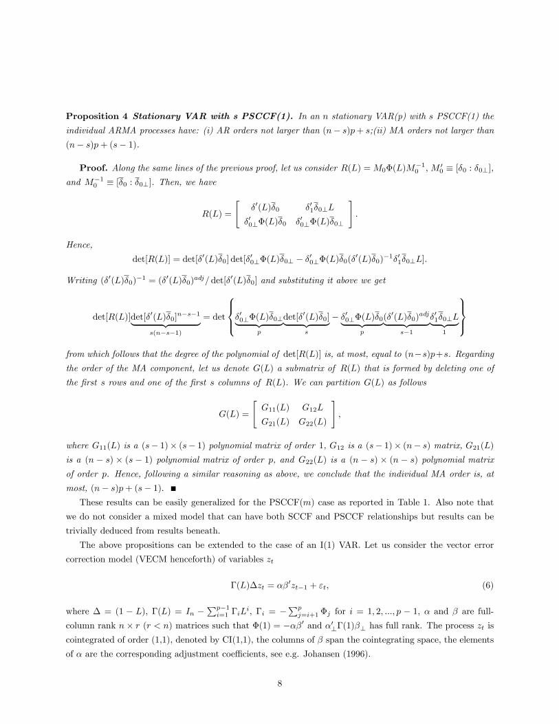
Figure 1: Quarterly growth rates of industrial production indexes (industrial sector)

­.08

­.06

­.04

­.02

.00

.02

.04

.06

1965 1970 1975 1980 1985 1990 1995 2000

Canadian growthAmerican growth

2.5 An example: Industrial output growth in Canada and the US

Engle and Kozicki (1993) �nd that there exists a SCCF relationship between the Canadian and the US

quarterly growth rates of output (seasonally adjusted series). They have considered a sample from the late

1950s to the late 1990s. We select the same countries and we use the seasonally adjusted industrial production

indexes from OECD main indicators over the period 1960:Q1-2004:Q3, namely we have 175 observations.

Figure 1 plots these series. The model selection criteria LR, AIC, HQ and SBC lead to selecting p = 2

for the log-levels of the bivariate processes. We reject the presence of cointegration at usual signi�cance

levels using Johansen�s trace test. Consequently the analysis is performed in �rst di¤erences, namely with

quarterly growth rates, with one lag only.

The estimation by OLS of the VAR(1) in �rst di¤erences delivers (standard errors in brackets)

" d� lnUSAtd� lnCAt

#=

264 0:003(0:001)

0:003(0:001)

375+264 0:333

(0:088)0:273(0:079)

0:265(0:102)

0:360(0:092)

375" � lnUSAt�1� lnCAt�1

#:

In order to check whether the coe¢ cient matrix is of reduced rank we compute a SCCF test statistics using

a canonical correlations approach (e.g. Vahid and Engle, 1993) between �zt = (� lnUSAt : � lnCAt)0

and �zt�1: The results are as follows: p � value = 0:31 is the p-value associated with the null hypothesis(�2(1)) that a linear combination of �zt is orthogonal to the past of �zt. Information criteria also lead to

14

select s = 1 (Hecq, 2006): The estimated common cyclical feature relationship is � lnUSAt � 1:05� lnCAt:Without any constraints on the short-run, both implied series should follow ARMA(2,1) processes. However,

the sample ACF and PACF indicate (�gures not reported in the paper) that the orders are probably shorter

and that AR(1) models for industrial production in both countries are more appropriate. For univariate

AR(1) models, the estimated equations have quite similar AR roots

d� lnUSAt = 0:003(0:001)

+ 0:554(0:062)

� lnUSAt�1;

d� lnCAt = 0:004(0:001)

+ 0:533(0:064)

� lnCAt�1;

where for both equations, the null of no disturbance autocorrelation is not rejected using LM tests.

One part of our story is con�rmed, i.e., the implied individual ARMA models have smaller AR orders

than those that we should get in absence of common feature restrictions and the two series exhibit one

signi�cant SCCF relationship. Moreover, the AR roots are similar for both countries. What might look

as evidence against our prediction is the absence of a MA component because both growth rates should be

ARMA(1,1).6 However, since � is close to (1 : �1)0, the variances of VAR residuals are similar, and the

correlation of VAR residuals is around 0.65, the results presented in Subsection 2.4 may explain why the

MA(1) components are almost negligible.

3 Estimation procedures for implied univariate models and mod-

elling considerations

As mentioned above, the �nding that a set of series have identical autoregressive polynomials is an indication

that these series have been generated by a VAR with non-(block)-diagonal and non-(block)-triangular matrix

�(L) and that beyond having this common univariate autoregressive polynomial, they share other common

features.7 This indication for the existence of common features calls for testing whether the moving average

part of the set of variables zit with identical autoregressive polynomials exhibits the multivariate index

structure implied by the presence of common features (see Subsection 2.4). A test of the multivariate index

structure could be carried out using the residuals of det[�(L)]zit. The properties of such a residual-based

test would be a¤ected by the properties of the estimator of the univariate autoregressive polynomials �i(L):

It is therefore important to estimate these polynomials as accurately as possible.

We address the problem of estimation and testing of univariate ARMA models implied by a VAR(p)

model with cofeature restrictions. Univariate ARMA models can be estimated in a straightforward way by

the maximum likelihood method, that is we identify and estimate by ML for each series individually the

6Using univariate maximum likelihood estimation, the MA(1) component has p-values of 0.16 and 0.32 for respectively theUS and Canada.

7Of course variables zit with di¤erent univariate autoregressive polynomials could be generated by di¤erent sub-systems ofa multivariate VAR with a corresponding block-diagonal matrix �(L):

15

parsimonious empirical ARMA(pi; qi) such that

zit = �i +�pij=1�ijzit�j +�

qik=1�ikuit�k + uit; i = 1 : : : n; t = 1 : : : T; (7)

where �i; �ij and �ik are estimated scalar parameters for series i; i 2 f1; 2; :::; ng; pi and qi are the lagorders of the ARMA model for the ith series and they might empirically di¤er from series to series. This

�rst stage of the analysis is helpful because we can get a �rst idea about a maximum AR order p as well as

of the number of series that might share co-movements.8 In doing so, we obtain a rough indication, a sort

of upper bound say, regarding the possible number of common feature vectors, with max(pi) = (n � s)p:Also, if for a series the AR order di¤ers much from that for other series, then probably it does not share a

common cycle with these other variables. Indeed, in absence of cancellation of common roots in the ARMA

representations, the �ij�s should be the same for all zit�s.

For sets of univariate ARMA models derived from a stationary multivariate ARMA model, Wallis (1977)

has considered maximum likelihood estimation, whereas Palm and Zellner (1980) have considered both

maximum likelihood and e¢ cient two-step estimation. For (di¤erence)-stationary series, the asymptotic

properties of univariate and multivariate estimation and test procedures are standard and known. For

integrated processes with or without cointegration present, when the unit root is not imposed, the asymptotic

procedures generally are non-standard. Whether standard asymptotics hold or not, likelihood and e¢ cient

two-step methods for systems may be cumbersome to implement when the set of variables is large. Therefore,

for empirical work, it will be useful to have tools at the disposal which can be easily implemented and lead

to reliable inference. Satisfying this need is the objective of this section.

3.1 Estimation of the common autoregressive polynomial using aggregates of

individual series

It has been emphasized in Section 2 that the series implied by the VAR must have the same AR coe¢ cients.

Consequently we investigate whether imposing this restriction using an estimator of the common AR part9

such that

zit = �i +�pij=1�jzit�j +�

qik=1�ikuit�k + uit; (8)

where �j is the jth lag order common coe¢ cient to all n that should be preferred to estimating ARMA

models for the individual series: In order to avoid new notation, we use the same symbols as in (7) for the

estimated intercept and moving average parameters.

The intuition underlying the use of (8) is twofold. First, under the null hypothesis, this is a correct way to

impose the commonality observed in di¤erent series. Secondly, under the alternative namely when including

a set of n1 variables that does not belong to the same multivariate process then, erroneously imposing a

8Note that even though we do not identify the VAR order, we may nonetheless have an idea about p. For instance, withannual data p is typically at most 4 but p = 2 is the most common choice in empirical applications, whereas for quarterly datap is rarely found to be larger than 9.

9Note that the common AR operator can be obtained by factorizing the AR-polynomials for the individual series into theproduct of the individual operators and then cancelling common factors (Lütkepohl, 2005, 496).

16

common AR root for the n�n1 variables induces autocorrelation in the error terms. As a result, the detectedorder of the MA part can be higher than those observed for individual components. But before tackling this

issue, we need to get estimates of the common AR component.

After having identi�ed and estimated the parsimonious empirical ARMA(pi; qi) by ML for each series

individually; one solution is to compute the average of n AR parameters such that �mg

j = n�1Pn

i=1 �ij ;

j = 1:::max(pi): However proceeding this way the homogeneity we have under the null is ignored. Moreover

the estimation of n equations by ML induces a lot of variability in the estimation of that average.

Instead, because the implied model for det[�(L)]�zt is at most a MA[(n� s)p)] model in the presence ofSCCF vectors for instance, we further use this observation and estimate an ARMA model for the average of

the n series in the ML estimation of

�zt = �� �pj=1�av

j �zt�j +�qk=1�k�t�k + �t; (9)

with �zt = n�1�ni=1zit the simple average of n series, �t being the innovation of the univariate ARMA(p; q)

for �zt and �k being the k-th lag parameter of the moving average part of �zt: In this second setting we might

use a LM test for no autocorrelation or graphical tools (i.e. ACF, PACF) on �t to check the white noise

hypothesis. A rejection of that null is a sign of misspeci�cation, namely that we have likely included in

the analysis a series that is not implied by the same system and consequently does not have the same �nal

equation or does not have features in common with the other series in the system and therefore has higher

degree AR and MA polynomials.

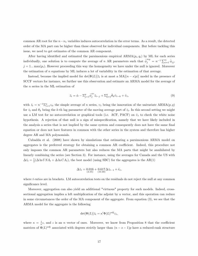
Cubadda et al. (2008) have shown by simulations that estimating a parsimonious ARMA model on

aggregates is the preferred strategy for obtaining a common AR coe¢ cient. Indeed, this procedure not

only imposes the common AR parameters but also reduces the MA parts that might be annihilated by

linearly combining the series (see Section 3). For instance, using the averages for Canada and the US with

��zt =12 (� lnUSAt +� lnCAt), the best model (using SBC) for the aggregates is the AR(1)

��zt = 0:016(3:55)

+ 0:617(10:40)

��zt�1 + et;

where t-ratios are in brackets. LM autocorrelation tests on the residuals do not reject the null at any common

signi�cance level.

Moreover, aggregation can also yield an additional "virtuous" property for such models. Indeed, cross-

sectional aggregation implies a left multiplication of the adjoint by a vector, and this operation can reduce

in some circumstances the order of the MA component of the aggregate. From equation (3), we see that the

ARMA model for the aggregate is the following

det[�(L)]�zt = �0�(L)adj"t;

where � = 1n �, and � is an n vector of ones. Moreover, we know from Proposition 8 that the coe¢ cient

matrices of �(L)adj associated with degrees strictly larger than (n� s� 1)p have a reduced-rank structure

17

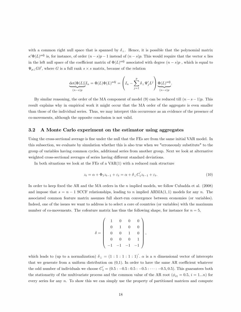
with a common right null space that is spanned by �?. Hence, it is possible that the polynomial matrix

�0�(L)adj is, for instance, of order (n� s)p� 1 instead of (n� s)p. This would require that the vector � liesin the left null space of the coe¢ cient matrix of �(L)adj associated with degree (n� s)p , which is equal top?G�

0, where G is a full rank s� s matrix, because of the relation

det[�(L)]| {z }(n�s)p

In = �(L)�(L)adj =

0@In � pXj=1

�?0jL

j

1A�(L)adj| {z }(n�s)p

:

By similar reasoning, the order of the MA component of model (9) can be reduced till (n� s� 1)p. Thisresult explains why in empirical work it might occur that the MA order of the aggregate is even smaller

than those of the individual series. Thus, we may interpret this occurrence as an evidence of the presence of

co-movements, although the opposite conclusion is not valid.

3.2 A Monte Carlo experiment on the estimator using aggregates

Using the cross-sectional average is �ne under the null that the FEs are from the same initial VAR model. In

this subsection, we evaluate by simulation whether this is also true when we "erroneously substitute" to the

group of variables having common cycles, additional series from another group. Next we look at alternative

weighted cross-sectional averages of series having di¤erent standard deviations.

In both situations we look at the FEs of a VAR(1) with a reduced rank structure

zt = �+�1zt�1 + "t = �+ �?C0

1zt�1 + "t: (10)

In order to keep �xed the AR and the MA orders in the n implied models, we follow Cubadda et al. (2008)

and impose that s = n � 1 SCCF relationships, leading to n implied ARMA(1; 1) models for any n. Theassociated common feature matrix assumes full short-run convergence between economies (or variables).

Indeed, one of the issues we want to address is to select a core of countries (or variables) with the maximum

number of co-movements. The cofeature matrix has thus the following shape, for instance for n = 5;

� =

0BBBBBBB@

1 0 0 0

0 1 0 0

0 0 1 0

0 0 0 1

�1 �1 �1 �1

1CCCCCCCA;

which leads to (up to a normalization) �? = (1 : 1 : 1 : 1 : 1)0: � is a n dimensional vector of intercepts

that we generate from a uniform distribution on (0,1): In order to have the same AR coe¢ cient whatever

the odd number of individuals we choose C0

1 = (0:5 : �0:5 : 0:5 : �0:5 : � � � : �0:5; 0:5): This guarantees boththe stationarity of the multivariate process and the common value of the AR root (�i1 = 0:5; i = 1:::n) for

every series for any n. To show this we can simply use the property of partitioned matrices and compute

18

det[I � �1L] when considering the (n � 1) � (n � 1) upper-left block of (I � �1L). We use M = 2000

replications of T + 50 observations before dropping the �rst 50 points to initialize the random sequence.

3.2.1 Experiment 1: Impact of adding series not generated from a VAR

In this �rst experiment we successively consider n = 5; 11; 23 series generated by the VAR (10) for T =

50; 100; 250. However, for the last n2 = (n � 1)=2 series, we substitute series generated by the followingdiagonal VAR:

yt = �1yt + "t; t = 1:::T; (11)

where �1 = diag( ) + U(�0:125; 0:125), and = 0; 0:25; 0:5. These are heterogeneous AR(1) processes

such that only when = 0:5 the coe¢ cient comes from an uniform distribution centered around the same

AR parameter of the FEs associated with (10). For the covariance matrix of the VAR errors we use in

this �rst experiment �" = I: This implies cross-correlated errors wt = �(L)adj"t in the FEs because their

contemporaneous covariance matrix is E(wtw0t) = I + �1�0

1: This corresponds to a correlation between the

disturbances of the implied equations of � = 0:55 for all pairs.

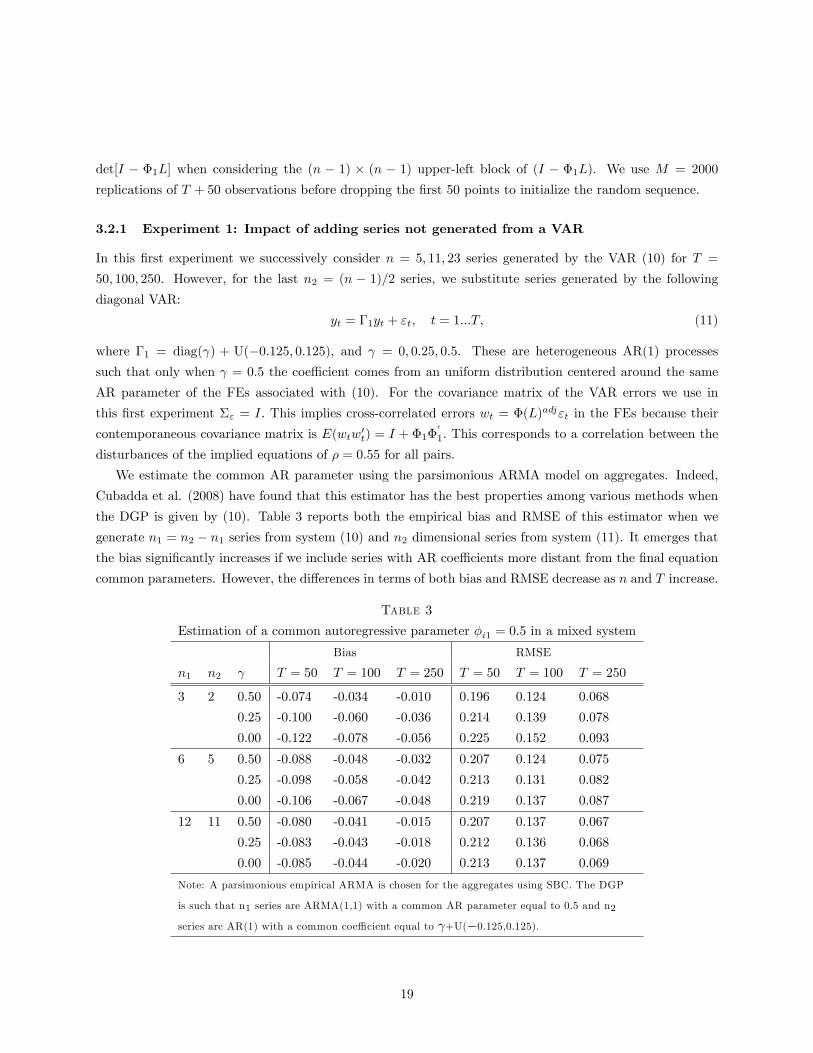
We estimate the common AR parameter using the parsimonious ARMA model on aggregates. Indeed,

Cubadda et al. (2008) have found that this estimator has the best properties among various methods when

the DGP is given by (10). Table 3 reports both the empirical bias and RMSE of this estimator when we

generate n1 = n2 � n1 series from system (10) and n2 dimensional series from system (11). It emerges that

the bias signi�cantly increases if we include series with AR coe¢ cients more distant from the �nal equation

common parameters. However, the di¤erences in terms of both bias and RMSE decrease as n and T increase.

Table 3

Estimation of a common autoregressive parameter �i1 = 0:5 in a mixed system

Bias RMSE

n1 n2 T = 50 T = 100 T = 250 T = 50 T = 100 T = 250

3 2 0:50 -0.074 -0.034 -0.010 0.196 0.124 0.068

0:25 -0.100 -0.060 -0.036 0.214 0.139 0.078

0:00 -0.122 -0.078 -0.056 0.225 0.152 0.093

6 5 0:50 -0.088 -0.048 -0.032 0.207 0.124 0.075

0:25 -0.098 -0.058 -0.042 0.213 0.131 0.082

0:00 -0.106 -0.067 -0.048 0.219 0.137 0.087

12 11 0:50 -0.080 -0.041 -0.015 0.207 0.137 0.067

0:25 -0.083 -0.043 -0.018 0.212 0.136 0.068

0:00 -0.085 -0.044 -0.020 0.213 0.137 0.069

Note: A parsimonious empirical ARMA is chosen for the aggregates using SBC. The DGP

is such that n1 series are ARMA(1,1) with a common AR parameter equal to 0.5 and n2

series are AR(1) with a common coe¢ cient equal to +U(�0.125,0.125).

19

3.2.2 Experiment 2: Simple vs. weighted averages

In this second experiment, we extend the Monte Carlo analysis of Cubadda et al. (2008) to allow for

heterogenous variances of the individual series. In particular, we now use in DGP (10) a covariance matrix

of the VAR �" such that its diagonal elements are (12; 22; :::; n2) and the correlation is equal to 0.7 for

any pair of errors. This implies a contemporaneous covariance matrix E(wtw0t) = �" + �1�"�0

1. We use

M = 2000 replications of n = 5; 11; 23 individuals with T = 50; 100; 250 observations after having discarded

50 points as starting values.

Since weighted averages are more appropriate than simple averages when series have di¤erent variances,

we compare the performances of four types of aggregates:

1. Av1 is a simple average of the series;

2. Av2 is a weighted average where the weights are proportional to the inverse of the unconditional

standard deviations of the series;

3. Av3 is a weighted average where the weights are proportional to the inverse of the conditional standard

deviations of the series �ui obtained through the estimated ARMA(1,1) models;

4. Av4 is a weighted average where the weights are proportional to the inverse of the standard deviationsq�2ui(1 + �

2i1) of the MA(1) innovations of the series obtained through the estimated ARMA(1,1)

models.

Table 4 reports the empirical bias and RMSE of the estimators of the common AR parameter for the

above aggregates. It emerges that the estimator based on Av4 has, overall, the best performance. The

intuition behind this �nding is that, since the MA component is noise in this estimation problem, the Av4weighted average gives more weight to less noisy series. However, the di¤erences in terms of performance of

the various estimators are not large, and they tend to disappear as both n and T become large.

20

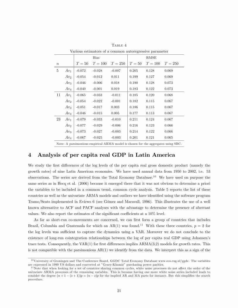
Table 4

Various estimators of a common autoregressive parameter

Bias RMSE

n T = 50 T = 100 T = 250 T = 50 T = 100 T = 250

5 Av1 -0.072 -0.028 -0.007 0.205 0.128 0.069

Av2 -0.054 -0.012 0.011 0.199 0.127 0.069

Av3 -0.046 -0.006 0.018 0.190 0.128 0.073

Av4 -0.040 -0.001 0.019 0.183 0.122 0.073

11 Av1 -0.065 -0.033 -0.011 0.185 0.120 0.068

Av2 -0.054 -0.022 -0.001 0.182 0.115 0.067

Av3 -0.051 -0.017 0.003 0.186 0.115 0.067

Av4 -0.046 -0.015 0.005 0.177 0.113 0.067

23 Av1 -0.079 -0.033 -0.010 0.211 0.124 0.067

Av2 -0.077 -0.029 -0.006 0.216 0.123 0.066

Av3 -0.073 -0.027 -0.003 0.214 0.122 0.066

Av4 -0.067 -0.025 -0.003 0.201 0.121 0.065

Note: A parsimonious empirical ARMA model is chosen for the aggregates using SBC.

4 Analysis of per capita real GDP in Latin America

We study the �rst di¤erences of the log levels of the per capita real gross domestic product (namely the

growth rates) of nine Latin American economies. We have used annual data from 1950 to 2002, i.e. 53

observations. The series are derived from the Total Economy Database.10 We have used on purpose the

same series as in Hecq et al. (2006) because it emerged there that it was not obvious to determine a priori

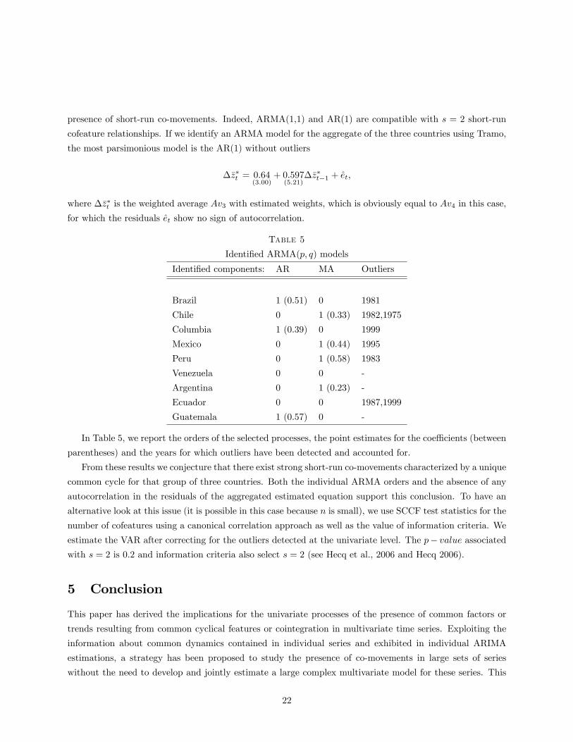
the variables to be included in a common trend, common cycle analysis. Table 5 reports the list of these

countries as well as the univariate ARMA models and outliers we have identi�ed using the software program

Tramo/Seats implemented in Eviews 6 (see Gómez and Maravall, 1996). This illustrates the use of a well

known alternative to ACF and PACF analyses with the advantage to determine the presence of aberrant

values. We also report the estimates of the signi�cant coe¢ cients at a 10% level.

As far as short-run co-movements are concerned, we can �rst form a group of countries that includes

Brazil, Columbia and Guatemala for which an AR(1) was found.11 With these three countries, p = 2 for

the log levels was su¢ cient to capture the dynamics using a VAR. Moreover we do not conclude to the

existence of long-run cointegration relationships between the log of per capita real GDP using Johansen�s

trace tests. Consequently, the VAR(1) for �rst di¤erences implies ARMA(3,2) models for growth rates. This

is not compatible with the parsimonious AR(1) we identify from the data. We interpret this as a sign of the

10University of Groningen and The Conference Board, GGDC Total Economy Database www.eco.rug.nl/ggdc. The variablesare expressed in 1990 US dollars and converted at �Geary-Khamis�purchasing power parities.11Note that when looking for a set of countries sharing common cycles, white noise processes do not a¤ect the order of the

univariate ARMA processes of the remaining variables. This is because having one more white noise series included leads toconsider the degree (n+ 1� (s+ 1))p = (n� s)p for the implied AR and MA parts for instance: But this simpli�es the searchprocedure.

21

presence of short-run co-movements. Indeed, ARMA(1,1) and AR(1) are compatible with s = 2 short-run

cofeature relationships. If we identify an ARMA model for the aggregate of the three countries using Tramo,

the most parsimonious model is the AR(1) without outliers

��z�t = 0:64(3:00)

+ 0:597(5:21)

��z�t�1 + et;

where ��z�t is the weighted average Av3 with estimated weights, which is obviously equal to Av4 in this case,

for which the residuals et show no sign of autocorrelation.

Table 5

Identi�ed ARMA(p; q) models

Identi�ed components: AR MA Outliers

Brazil 1 (0.51) 0 1981

Chile 0 1 (0.33) 1982,1975

Columbia 1 (0.39) 0 1999

Mexico 0 1 (0.44) 1995

Peru 0 1 (0.58) 1983

Venezuela 0 0 -

Argentina 0 1 (0.23) -

Ecuador 0 0 1987,1999

Guatemala 1 (0.57) 0 -

In Table 5, we report the orders of the selected processes, the point estimates for the coe¢ cients (between

parentheses) and the years for which outliers have been detected and accounted for.

From these results we conjecture that there exist strong short-run co-movements characterized by a unique

common cycle for that group of three countries. Both the individual ARMA orders and the absence of any

autocorrelation in the residuals of the aggregated estimated equation support this conclusion. To have an

alternative look at this issue (it is possible in this case because n is small), we use SCCF test statistics for the

number of cofeatures using a canonical correlation approach as well as the value of information criteria. We

estimate the VAR after correcting for the outliers detected at the univariate level. The p� value associatedwith s = 2 is 0.2 and information criteria also select s = 2 (see Hecq et al., 2006 and Hecq 2006).

5 Conclusion

This paper has derived the implications for the univariate processes of the presence of common factors or

trends resulting from common cyclical features or cointegration in multivariate time series. Exploiting the

information about common dynamics contained in individual series and exhibited in individual ARIMA

estimations, a strategy has been proposed to study the presence of co-movements in large sets of series

without the need to develop and jointly estimate a large complex multivariate model for these series. This

22

strategy is based on the theoretical results for the orders of the FEs for VAR models with co-features. The

strategy is shown to yield sensible results in an application involving GDP data for nine countries.

Many further developments are currently under investigations such as, inter alia, the development of

panel unit root tests and the extension to seasonal models. Moreover, the small sample and asymptotic

properties of the proposed methods must be more deeply evaluated.

The tools we introduce can be extended in several directions. For instance, they allow to study co-

movements between variables or convergence among economies, forecast series, and build business cycle

indices without requiring a full parametric system with many variables. The advantages of our approach are:

1) its feasibility when it is not possible to jointly analyze a complete system or when we prefer to work using a

sub-system, 2) its usefulness to detect sets of variables that are likely to be generated by seemingly unrelated

subsystems for subsets of variables that have some features in common, 3) the accuracy of forecasts, 4) the

ease of its implementation when a large number of jointly dependent variables has to be studied in complex

situations, 5) the potential empirical applications in many �elds.

Finally, the insights obtained from the analyses of single series and subset of series with identical AR parts,

and from testing for short-run and long-run co-feature restrictions can be incorporated in the multivariate

model for all series to be modeled.

References

[1] Ahn, S.K. (1997), Inference of Vector Autoregressive Models with Cointegration and Scalar Compo-

nents, Journal of the American Statistical Association, 92, 350-356.

[2] Bai, J. and S. Ng (2004), A PANIC Attack on Unit Roots and Cointegration, Econometrica 72,

1127-1177.

[3] Brüggemann, R., Krolzig, H.M. and H. Lütkepohl (2003), Comparison of Model Reduction

Methods for VAR Processes, Economics Papers #2003-W13, Economics Group, Nu¢ eld College, Uni-

versity of Oxford.

[4] Centoni M., Cubadda G., and A. Hecq (2007), Common Shocks, Common Dynamics, and the

International Business Cycle, Economic Modelling, 24, 149-166.

[5] Cubadda, G. and A. Hecq (2001), On Non-Contemporaneous Short-Run Comovements, Economics

Letters, 73, 389-397.

[6] Cubadda, G. (2007), A Unifying Framework for Analyzing Common Cyclical Features in Cointegrated

Time Series, Computational Statistics and Data Analysis, 52, 896-906

[7] Cubadda, G., Hecq, A. and F.C. Palm (2008), Macro-panels and Reality, Economics Letters, 99,

537-540.

[8] Engle, R.F. and S. Kozicki (1993), Testing for Common Features (with comments), Journal of

Business and Economic Statistics 11, 369-395.

23

[9] Ericsson, N., 1993, Comment (on Engle and Kozicki, 1993), Journal of Business and Economic

Statistics, 11, 380�383.

[10] Forni M., M. Hallin, Lippi M. and L. Reichlin (2000), The Generalized Dynamic Factor Model:

Identi�cation and Estimation, Review of Economics and Statistics, 82, 4, 540-554.

[11] Franses, P.H. (1998), Time Series Models for Business and Economic Forecasting, Cambridge Uni-

versity Press.

[12] Gómez, V. and A. Maravall (1996), Programs TRAMO (Time series Regression with Arima noise,

Missing observations, and Outliers) and SEATS (Signal Extraction in Arima Time Series). Instructions

for the User, Working Paper 9628, Research Department, Banco de España.

[13] Gouriéroux, Ch. and I. Peaucelle (1989), Detecting a Long-run Relationship, CEPREMAP Dis-

cussion Paper, 8902.

[14] Hecq, A. (2006), Cointegration and Common Cyclical Features in VAR Models: Comparing Small

Sample Performances of the 2-Step and Iterative Approaches, University of Maastricht Research Mem-

orandum.

[15] Hecq, A., Palm, F.C. and J.P. Urbain (2002), Separation, weak exogeneity and P-T decomposition

in cointegrated VAR systems with common features, Econometric Reviews, 21, 273�307.

[16] Hecq, A., Palm, F.C. and J.P. Urbain (2006), Common Cyclical Features Analysis in VAR Models

with Cointegration, Journal of Econometrics, 132, 117-141.

[17] Johansen, S. (1996), Likelihood-Based Inference in Cointegrated Vector Autoregressive Models (Oxford

University Press: Oxford).

[18] Lütkepohl, H. (2005), New Introduction to Multiple Time Series Analysis, Springer Verlag, Berlin.

[19] Maravall, A. and A. Mathis (1994), Encompassing Univariate Models in Multrivariate Time Series:

a Case Study, Journal of Econometrics, 61, 197-233.

[20] Palm, F.C. (1977), On Univariate Time Series Methods and Simultaneous Equation Econometric

Models, Journal of Econometrics, 5, 379-388.

[21] Palm, F.C. and A. Zellner (1980), Large-Sample Estimation and Testing Procedures for Dynamic

Equation Systems, Journal of Econometrics, 12, 251-283.

[22] Quenouille, M.H. (1957, 1968 2nd ed), The Analysis of Multiple Time-Series, Hafner Publishing

Co., New-York.

[23] Reinsel, G. (1983), Some Results on Multivariate Autioregressive Index Models, Biometrika, 70,

145-156.

24

[24] Schleicher, Ch. (2007), Codependence in Cointegrated Autoregressive Models, Journal of Applied

Econometrics, 22, 137-159.

[25] Stock J.H. and M.W. Watson (2002),Macroeconomic Forecasting Using Di¤usion Indexes, Journal

of Business and Economic Statistics, 20, 2, 147-162.

[26] Tiao, G.C. and R.S. Tsay (1989), Model Speci�cation in Multivariate Time Series (with comments),

Journal of Royal Statistical Society, Series B, 51, 157-213.

[27] Vahid, F. and R.F. Engle (1993), Common Trends and Common Cycles, Journal of Applied Econo-

metrics, 8, 341-360.

[28] Vahid, F. and R.F. Engle (1997), Codependent Cycles, Journal of Econometrics, 80, 199-221.

[29] Wallis, K.F. (1977), Multiple Time Series Analysis and the Final Form of Econometric Models,

Econometrica, 45, 1481-97.

[30] Zellner, A. and F.C. Palm (1974), Time Series Analysis and Simultaneaous Equation Econometric

Models, Journal of Econometrics, 2, 17-54.

[31] Zellner, A. and F.C. Palm (1975), Time Series and Structural analysis of Monetary Models of the

US Economy, Sanhya: The Indian Journal of Statistics, Series C, 37, 12-56.

[32] Zellner, A. and F.C. Palm (2004), The Structural Econometric Time Series Analysis Approach,

Cambridge University Press.

25