Nerve fiber conduction velocity distributions: Studies of normal and diabetic human nerves

634 Electroencephalography and Clinical Neurophysiology, 1979, 46:634--646 © Elsevier/North-Holland Scientific Publishers, Ltd.

NERVE FIBER CONDUCTION-VELOCITY DISTRIBUTIONS. I. ESTIMATION BASED ON THE SINGLE-FIBER AND COMPOUND ACTION POTENTIALS 1

KENNETH L. CUMMINS, DONALD H. PERKEL and LESLIE J. DORFMAN 2

(D.H.P.) Department of Biological Sciences, Stanford University, and Department of Neurology, Stanford University Medical Center, Stanford, Calif. 94305 (U.S.A.)

(Accepted for publication: September 29, 1978)

Clinical medicine relies in part on the elec- trophysiological properties of nerve and muscle for characterizing peripheral nerve funct ion in health and disease. The most commonly used measure of nerve funct ion is the conduct ion velocity (CV) of the fastest fibers in the nerve bundle. The objective of this paper is to demonstra te how nerve bundle conduct ion properties may be more com- pletely characterized using a general procedure for estimating the nerve fiber CV distribution from measurements of the nerve compound action potential (CAP).

A vast amount of knowledge concerning the electrogenesis of the CAP has been accumulated over the past half century. Gasser and Erlanger (1927) first described the quantitative principles relating nerve fiber diameter, CV, single-fiber action potential (SFAP), and the nerve bundle CAP. Gasser and Erlanger demonstra ted that a wave form similar to the recorded CAP could be 'recon- s t ructed ' using hypothesized SFAPs and measured fiber diameter distributions. Since that t ime, many investigators have studied the relationships and interdependencies among the parameters involved, yielding a rather dis- parate body of informat ion (Blair and Erlanger 1933; Zot terman 1937; Gasser and Grundfest 1939; Hursh 1939; Rushton 1951;

1 Supported by USPH Grant NS 09744 (D.H.P.) and by a grant from the Kroc Foundation (L.J.D.).

2 Reprint requests: Leslie J. Dorfman, M.D., Dept. of Neurology, Stanford University Medical Center, 300 Pasteur Drive, Stanford, Calif. 94305, U.S.A.

Paintal 1966). There is general consensus as to the basic parameters involved; however, there is little agreement about the quantitative relationships among CV, SFAP and fiber diameter. Discrepancies among the results obtained might be at t r ibuted to the varying recording techniques and instrumentat ion or to actual phylogenetic or class differences among the nerves under study. In either case, a unified general model of the CAP, capable of incorporating any of the proposed relationships, would be a useful tool for comparing various assumptions, accommodat ing variations in the nerves under study, and account- ing for changes in assumptions due to new and more accurate evidence.

This paper presents a model of the nerve CAP and a general procedure, based on this model, for estimating the distribution of CVs within a nerve bundle. A short discussion of previous related work by other investigators is given first, in order to place this work in historical context . Finally, we describe the application of the procedure both to experimental data of historical interest and to clinically derived CAPs.

Background of the estimation problem

Attempts have been made to estimate the distribution of fiber CVs in a nerve bundle using several different stratagems. Thomas et al. (1959) tried to determine the range of alpha moto r CVs by observing single motor unit action potentials after selective blockade of some descending impulses from a supra-

NERVE CONDUCTION-VELOCITY DISTRIBUTIONS. I 635

maximal shock. This blockade was achieved via 'collision' of orthodromic and antidromic impulses in the same nerve fibers. Improve- ments and extensions of this collision technique have been adopted for similar purposes by Hopf (1963) and Gilliatt et al. (1976). Juul-Jensen and Mayer (1966) studied slow motor fibers using low-level stimulation and bipolar needle recordings in the muscle. All the methods indicated above are based on the observability of individual motor unit action potentials, and therefore are not of general applicability. Leifer et al. (1977) developed a direct method for estimating motor nerve CV distributions based on a generalization of the collision scheme.

An alternative method for analyzing motor CV in humans was described by Lee et al. (1975). They first determined a 'mean motor unit action potential ' ; then, using histological data, they reconstructed an 'expected' muscle CAP. By varying the CV distribution in a systematic fashion, they observed the effects on the simulated muscle CAP. In this manner, they determined specific CV distributions that could give rise to certain pathological muscle CAPs. This type of analysis was also performed for sensory fibers by Buchthal and Rosenfalck (1971). These methods suffer from various technical problems, including complex experimental protocols, subjective computer-aided analysis, or inapplicability to sensory and mixed nerve studies.

Olson (1973) introduced a detailed mathematical model of the monopolarly recorded nerve CAP, and a related procedure for estimating the CV distribution. This procedure circumvents many of the pitfalls and limitations inherent in the earlier methods. The model and procedure developed in this paper represent extensions and elabora- tions of the concepts developed by Olson (1973). In this model, the various assumptions and findings in the literature may be viewed as affecting one of 3 parametric values. This construction unifies the study of the CAP by making each assumption a special case of a general model.

Model of the compound nerve action potential (CAP)

Fig. 1 depicts the general model of the CAP in terms of its 3 parameters: a finite set of SFAPs, delay elements and amplitude weighting coefficients. The CAP, in this case, results from single-pulse activation at some point along the nerve remote from the recording site. Simply stated, the CAP is a weighted sum of delayed SFAPs. Two assumptions allow us to utilize the structure shown:

(1) SFAP wave forms may be grouped into classes based on CV, where each class is considered to be well represented by a single known wave form.

(2) All fibers are considered to be activated at known times, and therefore have known delays for specified CVs.

The second assumption can be satisfied by activating the nerve bundle with a fast voltage or current pulse. Minor variations in activation time may be accounted for in the delays, as described below. The first assumption is the more critical, since without it a useful model of the CAP is not possible,.. There are no reports in the literature describing systematic variations in SFAP wave shape (for a given stable recording environment) with any factors other than fiber diameter and CV (Blair and Erlanger 1933; Paintal 1966). Given a fixed relationship between diameter and velocity, the first assumption is reasonable. In fact, most investigators have assumed that SFAP wave shape was independent even of velocity (Gasser and Erlanger 1927; Gasser and Grundfest 1937; Rushton 1951; Buchthal and Rosenfalek 1966).

Given these two assumptions, a mathematical statement of the CAP may be expressed as follows:

N

C(t) = ~ wifi(t -- di) (1) i = l

where C( t )= the observed CAP, as a func- t ion of time; N = the number of fiber classes;

636 K.L. CUMMINS ET AL.

SINGLE-FIBER ACTION POTENTIALS

DELAYS DELAYED ACTION WEIGHTING POTENTIALS COEFFICIENTS

~ , ~ ) . ~ . ~ " ~ ~ f l ( t -d l )

C(t)

C(t) = ~ wifi(t-di) i = 1

TIME

Fig. 1. Diagrammatic representa t ion of the c o m p o u n d nerve act ion potent ia l [C(t)] in terms of its cons t i tuent nerve fiber act ion potent ials and their conduc t ion characteristics. The wave form fi(t) is the single-fiber act ion potent ia l for fibers in conduc t ion veloci ty class i; the quan t i ty d i is the propagat ion t ime from act ivat ion site to recording site for fibers in class i, and w i is the ampl i tude weighting coeff ic ient for the delayed single-fiber act ion potent ia l f i ( t - di) , represent ing the ampl i tude con t r ibu t ion of fiber class i to the c o m p o u n d act ion potential . The c o m p o u n d act ion potent ia l is thus considered to be a weighted sum of delayed single-fiber act ion potentials .

wi = the amplitude-weighting coefficient for class i; f i ( t )= the SFAP for CV class i; di = the propagation delay for fibers in class i.

Parameters of the model

(A ) Velocity c lasses - segregation of SFAPs by CV

We assume that SFAP shape is a function of velocity only, for a given recording confi- guration and environment. We then divide the range of CVs into N classes. The division of these classes must be sufficiently fine so that the SFAP produced by each fiber in velocity class i (i = 1, 2, ..., N) is essentially indistin- guishable from that produced by any other fiber in its class. We denote this SFAP as fi(t) (Fig. 1). These action potential functions are normalized to a magnitude of one, with any amplitude dependence on CV incorporated into the weighting coefficients (wi). This

enables us to account for all amplitude-related factors with a single set of coefficients, which proves useful in implementing the estimation procedure. If, in practice, there are variations in the SFAPs of an individual class (for example, due to location within the nerve bundle or to local variations in fiber characteristics), the functions fi(t) are the corresponding expected values, in the usual sense.

(B) Delay elements -- factors affecting SFAP propagation times

The major factors determining the delay times, i.e., the time elapsed from the instant of nerve activation until the action potential arrives at the recording site, are the distance traveled along the nerve and the velocity of propagation. In the case where CV in a fiber varies along the nerve, an average CV is used. Ideally, the delay values may be obtained from the equation

di = L / v i (2)


where di = de lay t ime fo r f ibers in ve loc i ty c lass i ; L = m e a s u r e d d i s tance f r o m the s t imula t ing c a t h o d e to the record ing site; v~ = the CV r ep re sen t ed b y ve loc i ty class i.

In general , t w o fac tors m a y m o d i f y the delays expressed in eqn. (2). When an e x t r e m e l y high s t imulus in tens i ty is used, the a p p a r e n t ac t iva t ion site, or 'v i r tua l c a t h o d e ' , m a y no t c o r r e s p o n d to the loca t ion of the ca thoda l e l ec t rode (Wiederhol t 1970) . F o r s t imulus intensi t ies ranging b e t w e e n 2 and 20 t imes m a x i m a l , exc i t a t i on o f the fas tes t f ibers m a y occu r at 1--2 c m f r o m the ca thode . This e f f ec t is m u c h less p r o n o u n c e d wi th lower s t imulus levels. Gi l l ia t t et al. (1965) obse rved de lay var ia t ions on the o rder o f 0 . 0 5 - O . 1 5 msec for s t imulus intensi t ies b e t w e e n th resho ld and 25% above t h a t requi red for m a x i m a l CAP a m p l i t u d e , as measured a t the e lbow. I t is r easonab le to assume t h a t this p h e n o m e n o n a f fec t s f ibers o f differ- en t CV classes unequa l ly (Gasser and Er langer 1939) , and t h e r e f o r e a var iable co r r ec t ion f ac to r m igh t be inc luded for each d~.

T h e second f a c t o r a f fec t ing the de lay mea- sures is the ac t iva t ion t ime for elicit ing a p r o p a g a t i n g ac t ion po ten t i a l . Blair and Er langer (1935) f o u n d t h a t this ac t iva t ion t ime was an e x p o n e n t i a l f unc t i on of s t imulus in tens i ty , a p p r o a c h i n g zero fo r inf ini te vol tage or cu r ren t , and close to 0.2 msec fo r a level twice the abso lu te th resho ld vol tage for a given f iber . A co r r e s pond i ng delay correc- t ion t e r m for this ac t iva t ion t ime can be inc luded in the model . I t wou ld be largest ( 0 . 2 - 0 . 4 msec) for higher t h r e sho ld (generally s lower conduc t ing ) f iber classes, and wou ld a p p r o a c h zero for the fas tes t f ibers, due to the i r l ower exc i t ab i l i ty th resho lds (Dawson 1956; Wiederhol t 1970) . Thus , the general express ion for the delays b e c o m e s

d i = (L --~i)/Vi + dai (3)

whe re ~i = v e l o c i t y - d e p e n d e n t c o r r e c t i o n fo r vi r tual c a t h o d e effects ; dai = e x p e c t e d activa- t ion t ime fo r f ibers in c!ass i.

In prac t ica l t e rms , r ecord ing dis tances are

o f t en long enough t h a t ~i m a y be cons ide red a c o n s t a n t and dai m a y be ignored :3

(C) Weighting coefficients -- factors affecting fiber class amplitude

T h e weight ing coef f ic ien t s (wi) are general p a r a m e t e r s to a c c o u n t for all inf luences on the c o n t r i b u t i o n of each f iber class to the observed CAP. Since the a m p l i t u d e of the SFAP m a y va ry f r o m class to class, w i has a f ac to r A(vi) to a c c o u n t for this d e p e n d e n c e . T h e c o n t r i b u t i o n o f the f ibers in class i t o the CAP will also be in f luenced b y the n u m b e r o f f ibers in the class (mi); this d e p e n d e n c e is d e n o t e d H(mi ) . T h u s wi m a y be expressed as

Wi = A(v i )H(mi )

mi = Mp(vi) (4)

where M = the t o t a l n u m b e r o f f ibers activa ted in the nerve bund le ; mi = the n u m b e r o f f ibers ac t iva ted in class i (E mi = M); A(vi) = SFAP a m p l i t u d e d e p e n d e n c e on CV; H(mi) = func t iona l d e p e n d e n c e o f the weigh t ing coef f ic ien t s on the n u m b e r o f f ibers in class i; p(vi) = the i ' th e l e m e n t o f the n o r m a l i z e d CV d i s t r ibu t ion (E p ( v i ) = 1) . The :Fraction of f ibers in class i, p(vi) , is the u n k n o w n pa rame- te r o f in teres t fo r each CV class. A(vi) repre- sents any a m p l i t u d e d e p e n d e n c e of the SFAPs in a given class on the CV. This par- t icular f unc t i on has been assigned d i f f e ren t

3 Virtual cathode effects and activation time may have little influence on the delay if conduction distances are long (Cummins 1977). Based on data by Buchthal and Rosenfalck (1966), in agreement with Wiederholt (1970), a constant value of 0.75 cm for ~i will introduce errors in CV of less than 2.5% for a conduction distance of 20 cm and stimulus levels up to 3 times that required for maximal CAP amplitude. Activation time will have even less effect. For a 20 cm conduction distance, errors in CV resulting from ignoring activation time will be no greater than 2%. Finally, the two phenomena act in opposition to each other, thus minimizing their combined effect.


forms by different investigators. Gasser and Erlanger (1927), Rushton (1951) and Buchthal and Rosenfalck (1966) all considered SFAP amplitude propor t ional to the square of the CV, whereas a linear rela- t ionship between SFAP ampli tude and CV was assumed by Blair and Erlanger (1933) and Gasser and Grundfest (1939). In modeling transfer characteristics of nerve bundles, Williams (1972) considered ampli tude to be independent of CV. In our general model, any explicit funct ion for A(vi) may be chosen.

The term H(mi) denotes the influence of the number of fibers in CV classi on the amplitude contr ibut ion of that class to the CAP. In most cases (Gasser and Erlanger 1927; Gasser and Grundfest 1939; Buchthal and Rosenfalck 1966; Olson 1973) this func- t ion is assumed to be simply mi, implying a linear cont r ibut ion of each nerve fiber to the total response. Buchthal (1973) and Tackmann et al. (1976) presented data on the sural nerve suggesting that the amplitude of the CAP increased as the logarithm of the number of fibers. In this case H(mi) would be proportional to log(mi). A third possibility (Lambert and Dyck 1975) is that amplitude may be proport ional to the density of fibers in each class. Assuming the nerve bundle to have a homogeneous distribution of fibers th roughout , H(mi) would then be simply cmi, where c is a positive constant.

Estimating the CV distribution

The CAP model of eqn. (1) can be formu- lated in terms of discrete time by using equally spaced samples for the SFAP and CAP functions. The discrete form is

N

C(tk) = ~ w i f i ( t k - -d i ) (5) i = l

where tk is the k ' th discrete (equally spaced) time point. From this equation, it can be seen that each time sample of the CAP [C(tk)] is a linear combinat ion of single const i tuents from

each CV class. Assuming that there are K values of the CAP, eqn. (5) may be writ ten in matrix form

c = Fw (6)

where c = a K × 1 column vector composed of K time samples of the CAP {C(tl), C(t2) ..., C(tK)} ; F = a K X N matrix whose i ' th column is the sampled SFAP funct ion fi(tk -- di); w - a N × 1 column vector of the N weighting coeff ic ients {Wl, w2 . . . . . WN}.

In terms of estimating the CV distribution from a measured CAP and known SFAP properties, eqn. (6) may be viewed as a set of K equations in N unknowns (the vector w). If the matrix F were square (i.e., if K = N) and non-singular, it would be possible in principle to solve eqn. (6) directly for the vector w. In practice, however, reasonable choices for CV classes can lead to a singular matrix F. Even if non-singular, the solution would be highly sensitive to noise in the CAP measurement and to minor variations in parameter values. Instead, we require the number of time samples to exceed the number of velocity classes (i.e., K > N). The system of simultaneous linear equations is then overdeter- mined. The matrix expression for the CAP readily allows a least-squares fit to be found for the vector w. It is a well known proper ty of such systems (Greville 1959) that the least- squares solution for the vector w, if the matrix F has rank N, is obtained by premulti- plying both sides of eqn. (6) by the transpose of the matrix F:

FTc = FTFw (7)

and solving to obtain the least-squares estimate of the weighting coefficients

V¢ = [FTF]- IFTc (8)

The columns of the matrix F are independent, as they are the sampled SFAPs having different delay times. Therefore , the N f N matrix FTF invariably has an inverse. The product [FTF]-I F T is of ten called the pseudoinverse of F (Penrose 1955; Greville 1959; Luenberger 1969). In practice, it is not


necessary to invert FTF to solve the system of eqn. (7); one may use any convenient stan- dard algorithm for solving simultaneous linear equations.

Since the number of equations to be solved is the same as the number of velocity classes (N), it follows that increasing the precision of time sampling (increasing K) does not increase the size of the system of equations to be solved. It does serve to improve the least- squares solution, by reducing the effects of time sampling.

The formulation described above yields a unique, closed-form estimate of the weighting coefficients (wi) in the general CAP model, and is readily implemented on a computer. In the examples to be discussed below, we solved eqn. (7) using Gaussian elimination (Forsythe and Moler 1967). The program was written in Fortran and run on a Digital Equipment Corporation PDP 11/34 computer.

Once the weighting coefficients are determined, eqn. (4) must be solved to obtain the normalized CV distribution. The advantage of grouping all the amplitude-related factors into one set of weighting coefficients becomes apparent here. The same optimal solution for the weighting coefficients can be used for a variety of assumed forms for the dependence of amplitude on fiber density and CV. An unique normalized CV distribution can be recovered through eqn. (4) as long as H ( m i ) is a monotonic function of m i. Almost any imaginable (physically meaningful) function H(.) meets this requirement.

One final point of interest is that M, the actual number of nerve fibers activated, will not, in general, be known; nor will the abso- lute amplitudes of the individual SFAPs. When H(mi) is proportional to the number of fibers in each class, as usually assumed, both of these factors are simply scaling constants. When at tempting to recover only the normalized CV distribution, these constants have no effect on the results.

In order to determine how well an observed CAP is matched by the model and the estimated CV distribution, the CAP can be

reconstructed using the F matrix created during the estimation procedure, together with the least-squares estimate of the vector w, using eqn. (6).

Application of the method

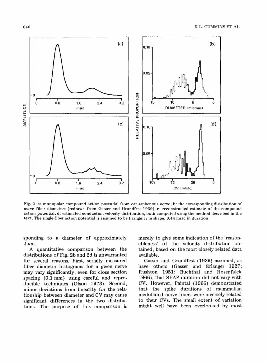
Some examples of the use of our model and estimation procedure are presented in Figs. 2, 3 and 4, using data of historical interest. The CAP and fiber diameter distribution in Fig. 2a and 2b, respectively, are redrawn from Gasser and Grundfest (1939, Figs. 5 and 7, cat saphenous nerve). They reconstructed the CAP of Fig. 2a using a triangular SFAP (0.44 msec duration), the diameter distribution of Fig. 2b, and the fol- lowing assumptions: (a) CV varies linearly with fiber diameter, and (b) SFAP amplitude increases linearly with CV (and thus linearly with fiber diameter). Gasser and Grundfest 's reconstruction was remarkably similar to the original CAP wave form when 'corrected' for irregularities which they assumed were due to variations in axon-to-outside diameters.

Fig. 2d is an estimated CV distribution, derived utilizing Gasser and Grundfest 's SFAP to construct the F matrix for eqn. (8). In this case, virtual cathode effects were significant due to the short conduction distance (4 cm). This was compensated for in the CAP wave form by Gasser and Grundfest (p. 405). The irregularity of the late portion o1! the reconstructed CAP in Fig. 2c is related to the CV class interval selected. A smaller interval would have given a smoother reconstruction.

The estimate of the CV distribution was calculated and plotted to allow a general comparison with the fiber diameter distribution in Fig. 2b. The CV axis in Fig. 2d was scaled in accordance with Gasser and Grundfest 's con- version factor of 7 .14m/sec per pm of diameter. The major difference between the two distributions involves the slowest fibers. Due to the brief duration of the CAP (3.2 msec, Fig. 2a), there are no fibers conducting more slowly than 14.5 m/sec, corre-


L~J £3

l-- m -J 0-

<

-0 !

0

(a)

I I I I

0.8 1.6 2.4 3.2 msec

(c)

n i ! 0.8 1 6 2.4 msec

-o J I I 0 3.2

a .

uJ > I . - < .,J LIJ

0.10-

D.05-

15

0.I0~

!

0.05-

10 5

DIAMETER (microns)

Y .d ! I

108 72 36

CV (m/sec)

(b)

(d)

Fig. 2. a: monopolar compound action potential from cat saphenous nerve; b: the corresponding distribution of nerve fiber diameters (redrawn from Gasser and Grundfest 1939); c: reconstructed estimate of the compound action potential; d: estimated conduction velocity distribution, both computed using the method described in the text. The single-fiber action potential is assumed to be triangular in shape, 0.44 msec in duration.

sponding to a diameter of approximately 2 pm.

A quantitative comparison between the distributions of Fig. 2b and 2d is unwarranted for several reasons. First, serially measured fiber diameter histograms for a given nerve may vary significantly, even for close section spacing (0.1 mm) using careful and repro- ducible techniques (Olson 1973). Second, minor deviations from linearity for the relationship between diameter and CV may cause significant differences in the two distributions. The purpose of this comparison is

merely to give some indication of the 'reason- ableness' of the velocity distribution obtained, based on the most closely related data available.

Gasser and Grundfest (1939) assumed, as have others (Gasser and Erlanger 1927; Rushton 1951; Buchthal and Rosenfalck 1966), that SFAP duration did not vary with CV. However, Paintal (1966) demonstrated that the spike durations of mammalian medullated nerve fibers were inversely related to their CVs. The small extent of variation might well have been overlooked by most


early investigators. We have studied the sensitivity of our model to different assumptions about SFAP duration. Fig. 3a, c and e show 3 different 'assumed' SFAPs. They each have a 1 : 2 ratio of rise time to fall time. The

Z (a)

o ~ - o'~ o~o o~.~ o~o ,mec

(b)

O~

108 72 36 CV q~,l,sec~

o ~ (c)

015 030 045 060 msec

-0 ~ (e)

/ 0 0 10 030 (] 45 0.60 mse¢

06] (g}

~°~1 ~o~

°'~ ,'0 4b ~'o 0'0 C V {m/sec}

01

J I z 108 72 36 ~0 C V (m/see)

0 1

8 CV ( m,'~ec )

Ol

, i

CV Im/sec}

(d)

(h)

Fig. 3. Effect of single-fiber action potential duration on the conduction velocity distribution. The compound action potential of Fig. 2a interacts with 3 hypothetical single-fiber action potentials of different durations (a, c, e), giving rise to the 3 corresponding conduction velocity distributions (b, d, f). If single-fiber action potential duration is permitted to vary with conduction velocity as shown in g (redrawn from Paintal 1966), the distribution in h is obtained.

SFAP in Fig. 3c is the one assumed by Gasser and Grundfest (1939) , having a duration of 0 .44 msec. In Fig. 3a, the SFAP is shorter in duration (0.34 msec), while in Fig. 3e the SFAP is longer (0.54 msec). Using the CAP from Fig. 2a, the effects o f these differences in SFAP duration are shown in the corresponding CV distributions of Fig. 3b, d and f. The CV class interval widths in Fig. 3 were set at 3.5 m/sec (as compared to 1.75 m/sec in Fig. 2d), to yield slightly smoother CV distribution estimates, making it easier to observe changes due to the varied SFAP parameters.

The conformations of the CV estimates in

0.11i = 0.0 (a)

8 0

: 1,0 0.2-

0,1-

108 72 36

0"1 I=2"0

0.2-

(b)

(c)

o

108 72 36 C V ( m / s e c )

Fig. 4. Influence of the single-fiber action potential amplitude exponent (the exponent, n, in A(vi )= cv n) on the conduction velocity distribution of Fig. 3d. In a, single-fiber action potential amplitude is independent of velocity. In b, amplitude is linearly related to conduction velocity. In c, amplitude is proportional to the square of conduction velocity.


Fig. 3b, d, and f have 3 basic differences. The most obvious difference is the height of the slow-fiber peak (15--35m/sec) . As SFAP duration increases from 0.34 to 0.54 msec, the proportion of slow fibers increases from 0.13 to 0.195. A more subtle change takes place in the proportion of fibers conducting between 40 and 70 m/sec. This proportion decreases monotonical ly as duration is increased and reflects the increasing area

under the SFAP functions as duration increases. The final point of interest is the 'smoothness ' of the distributions. As the SFAP is made wider, there are more fluctua- tions between adjacent velocity classes, particularly for the mid-range fibers. This phenomenon occurs regularly when the SFAP is too wide. In extreme cases, large negative values appear in the CV distribution, indicating an 'a t tempt ' by the estimation proce-

SFAP NORMAL CAP ABNORMAL CAP

o vL AlO VI

(c) (d ) (e) 0.30- ( i )

[[.. 0.15- t -

o o o o - ,-

a .

7- o.2o- (j) <

( f ) (g) (h ) -J

0"10"

o .o , , ,

70 515 40 25

I I CV (m/sec) 2 msec

Fig. 5. Conduc t ion veloci ty dis tr ibut ions derived f rom normal and abnormal c o m p o u n d act ion potentials, a, normal; b, abnormal human sensory c o m p o u n d act ion potent ials ; and c, ' assumed ' single-fiber act ion potentials , redrawn f rom Buchthal and Rosenfa lck (1971). Appl ica t ion of the es t imat ion procedure to these data yields the conduc t ion veloci ty dis t r ibut ions shown in i and the recons t ruc ted c o m p o u n d act ion potent ia ls in d and e. The cont inuous , open dis t r ibut ion in i corresponds to the normal c o m p o u n d act ion potent ial , whereas the inter- rupted, shaded dis t r ibut ion corresponds to the abnormal c o m p o u n d act ion potent ial , g, h, j, recons t ruc ted compound act ion potent ia ls and conduc t ion ve loc i ty dis tr ibut ions obta ined using the modif ied single-fiber act ion potent ia l in f. In both cases, the dis t r ibut ions derived f rom the abnormal c o m p o u n d act ion potent ia l are shifted toward the s lower conduc t ion velocities.


dure to compensate for the wide SFAPs. The CV distribution in Fig. 3h was also ob-

tained from the data of Gasser and Grundfest (1939). In this case, the SFAP form remained triangular, but its duration was assumed to vary with CV as described by Paintal (1966). The duration function is shown in Fig. 3g, as redrawn from Paintal (Fig. 2, p. 796) for cat saphenous nerve at 37.1 ° C.

In terms of the model of eqn. (5), the various examples shown in Fig. 3 demonstrate manipulations of the functions fi(tk). For Fig. 3a, c, and e, fi(tk) is independent of the CV class index i. In Fig. 3g, the class index determined the duration of fi(tk) through its velocity.

These results indicate that changes in SFAP characteristics do affect the CV distribution. However, variations as large as 20--30% in duration may cause only minor changes in the distribution.

The effects of different amplitude functions, denoted n ( v i ) in eqn. (4), are demonstrated in Fig. 4, using the SFAP of Fig. 3c. The exponent expressed in each element of the figure is the value specifying A(vi) = cvni, where c is an arbitrary positive constant. It is obvious from Fig. 4 that the exponent dra- matically alters the CV distribution estimate. Note, however, that the exponent does not alter the basic shape of the distribution. Therefore, erroneous assumptions about A(vi), if applied uniformly to all nerves under study, would not affect the ability of the distribution estimate to characterize variations among nerve bundles.

Discussion

The procedure for estimating the CV distribution of nerve fibers based on measurement of the CAP can incorporate the model presented in this paper in its most general form. The specific model parameters in the examples reflect assumptions made by the original investigators, and are not constraints on the estimation procedure. It is important

to emphasize that we do not estimate the fiber diameter distributions of the nerves under study. In part, this is due to the sensitivity of any model to the CV: diameter relationship. More important , it is fiber CV, not diameter, which most closely reflects nerve function in the clinical sense (Sharma and Thomas 1974).

There are some factors which could affect the general applicability of the model and procedure presented. It is possible that variability in SFAP wave shape among fibers in a single CV class might be too great to be characterized by a single function fi(t). In this case, the first assumption required for the model would be violated. From the example presented, it would seem that the variability in SFAP duration would have to be on the order of 20% to be significant. A second factor affecting the model as stated would be the occurrence of a nonmonotonic function for H(mi). In such a case, the CV distribution could not be recovered from knowledge of the weighting coefficients, because a single value for wi could be associated with two or more values of mi. In practice, one would expect H(mi) to be monotonic, such as a linear or logarithmic function.

There are several practical points pertaining to the application of the estimation procedure. First, it is desirable to pick the longest possible distance between stimulating and recording sites along the nerve. This will minimize sensitivity to measurement of conduction distance. Also, it might allow one to neglect virtual cathode and activation time effects, as their contributions become less significant with increasing delay time. Another important detail is the choice of CV class size. If the class divisions are defined too coarsely, the reconstructed CAP will be excessively irregular, indicating a poor fit. For this reason, it is advisable in implementations to compute and display the reconstructed CAP. On the other hand, too fine a division may result in an excessive number of weighting coefficients, increasing the computat ional burden. Not only must the


number of weighting coefficients remain less than the number of time samples of the CAP (allowing the least-squares fit), but also the velocity classes must be broad enough to insure that no two columns of the F matrix are identical. In our experience, appropriate choice of class intervals rapidly becomes obvious. In some cases, one may choose to have varying class intervals, allowing more detail in desired areas of the distribution.

The selection of wave form for the SFAPs may pose a problem, particularly when the method is applied to non-invasive clinical studies. Kovacs et al. (1977), using a related method for estimating the CV distribution, proposed the response to low-intensity electrical nerve stimulation as an estimate of the SFAP. As previously discussed, excessively broad SFAPs result in an unreasonable number of negative values in the recovered CV distribution. We have purposely not con- strained the estimates to be non-negative, in order to facilitate recognition of faulty model specifications. In the CAP of Gasser and Grundfest, the question of variation of SFAP duration with CV did not appear terribly important; however, in surface recordings, where SFAP wave shapes may be complex, accurate information about SFAP wave shapes becomes more important and less accessible.

An example of this problem is demonstrated in Fig. 5. The sensory CAPs in Fig. 5a and b are redrawn from Buchthal and Rosenfalck (1971, Fig. 2, p. 245). The smaller amplitude and longer latency of the abnormal CAP (Fig. 5b) may be accounted for by a 20% slowing in all fibers, as concluded by the original authors. Fig. 5i shows the CV distributions obtained with our estimation procedure, using the SFAP (Fig. 5c) and assumptions of Buchthal and Rosenfalck (1966, p. 95). The CV distribution of the abnormal CAP (shaded area) is shifted toward the right. However, the irregularity of the CV distribution appears excessive and indicates that the assumed SFAP is probably too wide.

The assumed SFAP in Fig. 5f is slightly

narrower than that in Fig. 5c and its details are more realistic. Using this SFAP and the same CAP data as above, we obtained the CV distributions in Fig. 5j. Note the increased smoothness and the virtual elimination of negative values in these histograms. They clearly indicate that the abnormal nerve (shaded area) has a reduced number of fibers conducting more rapidly than 40 m/sec, and an overall shift of fiber CVs to the slower velocity classes. The reconstructed CAPs in Fig. 5g and h were derived using the SFAP in Fig. 5f and the CV distributions in Fig. 5j. They are slightly 'rougher' than those in Fig. 5d and e (derived from the SFAP of Fig. 5c and the distributions of 5i), due to the narrower SFAP.

It is not possible to determine from the CV distributions alone whether there is a general slowing of conduction in all fibers of the abnormal nerve, or a selective loss (block) of the faster fibers. This could be determined only if the normal and abnormal CAPs were recorded with electrically identical electrodes at the same distance from the nerve, therefore allowing comparison of non-normalized CV distributions. It is well demonsl;rated, however, that the differences between the normal and abnormal CAPs occur as a result of dramatic differences in the CV distributions of the two nerves under study.

As illustrated above, the estimates of CV distribution are somewhat sensitive to poly- phasic SFAP wave shapes. This should be kept in mind when selecting a specific recording method, which will have some bearing on the complexity of the SFAPs. With purely monopolar (referential) recording, the SFAPs are often biphasic (Brown 1968; Plonsey 1974). With bipolar recordings, the SFAPs are generally triphasic, having various ratios of first positive peak to second positive peak, depending on electrode locations. Also, with bipolar recording, an explicit dependence of SFAP wave shape on CV is introduced, because potentials recorded in this manner represent the difference between two monopolar SFAPs recorded at a fixed spacing


(Hill 1934}. This d e p e n d e n c e can be expl ic i t ly a c c o u n t e d for , b u t will increase the d i f f i cu l ty o f SFAP spec i f ica t ion . I f the a p p r o p r i a t e SFAPs are k n o w n , t hen the p r o c e d u r e presented here can be readi ly i m p l e m e n t e d in prac t ica l app l ica t ions .

In a c o m p a n i o n p a p e r ( C u m m i n s et al. 1979) , we descr ibe a m e t h o d fo r e s t ima t ing the CV d i s t r ibu t ion (again based on the m o d e l deve loped in this paper}, which does n o t require expl ic i t k n o w l e d g e o f the SFAPs, bu t does requi re two m e a s u r e m e n t s o f the CAP at d i f f e ren t loca t ions a long the nerve. We con- sider the la t te r t e chn ique , by v i r tue of its i n d e p e n d e n c e f r o m k n o w l e d g e o f the SFAPs, to have grea ter po t en t i a l prac t ica l app l i ca t ion in the diagnosis and assessment of pe r iphera l nerve diseases. Howeve r , each m e t h o d has its o w n advan tages and special appl ica t ions .

d u c t i o n de la f ibre nerveuse dans un faisceau ne rveux . Ce t t e m ~ t h o d e est bas~e sur un modu le g~n~ral d~taill~ du po t en t i e l d ' a c t i o n global du fa isceau ne rveux , qui est caract~ris~ pa r la s o m m e pond~r~e des po ten t i e l s d ' a c t i o n re tard~s des f ibres isol~es. Ce t t e m ~ t h o d e d ' e s t i m a t i o n non- i t~ra t ive est appl iqu~e deux exemple s pris dans la l i t t~ra ture exi- s t an te p o u r m o n t r e r la similarit~ en t re vitesse de c o n d u c t i o n et d i s t r ibu t ion des d iam~tres des fibres, la sensibilit~ des mesures ~ des var ia t ions des pa ram~t res i m p o r t a n t s du mo- dule, et l ' appl icabi l i t~ de la d i f f~renc ia t ion de la f onc t i on du ne r f n o r m a l et ano rma l .

We thank Michael A. Hatfield for help with a preliminary version of this technique. We also thank Nicholas T. Carnevale for his helpful suggestions and review of the manuscript.

S u m m a r y

A m e t h o d is descr ibed for e s t ima t ing the d i s t r ibu t ion o f nerve- f iber c o n d u c t i o n veloci- t ies in a nerve bund le . This m e t h o d is based on a deta i led general m o d e l o f the nerve bund l e c o m p o u n d ac t ion po ten t i a l , which is cha rac te r i zed as a we igh ted sum of de l ayed single-f iber ac t ion po ten t ia l s . T h e non- i t e ra t ive e s t ima t ion m e t h o d is app l ied to t w o e x a m p l e s t a k e n f r o m exis t ing l i t e ra ture , d e m o n s t r a t i n g the s imi lar i ty o f c o n d u c t i o n ve loc i ty and f iber d i a m e t e r d i s t r ibu t ions , sens i t iv i ty o f the esti- m a t e to va r ia t ions in i m p o r t a n t m o d e l p a r a m - eters , and app l icab i l i ty to t he d i f f e r en t i a t i on o f n o r m a l and a b n o r m a l nerve func t ion .

R~sum~

Distr ibut ion des vitesses de conduc t i on de la fibre nerveuse. I. Es t imat ion basde sur les po ten t i e l s d 'act ion unitaires et g lobaux

Les au teurs d~cr ivent une m ~ t h o d e d 'es t i - m a t i o n de la d i s t r ibu t ion de la vi tesse de con-

Re fe r ences

Blair, E.A. and Erlanger, J. A comparison of the characteristics of axons through their individual electrical pulses. Amer. J. Physiol., 1933, 106: 524--564.

Blair, E.A. and Erlanger, J. On the process of excita- tion by brief shocks on axons. Amer. J. Physiol., 1935, 114: 309--316.

Brown, B.H. Theoretical and experimental waveform analysis of human compound nerve action potentials using surface electrodes. Med. Biol. Engng, 1968, 6: 376--386.

Buchthal, F. Sensory and motor conduction in poly- neuropathies. In: J.E. Desmedt (Ed.), New Devel- opments in Electromyography and Clinical Neuro- physiology, Vol. 2. Karger, Basel, 1973: 259--271.

Buchthal, F. and Rosenfalck, A. Evoked action potentials and conduction velocity in human sensory nerves. Brain Res., 1966, 3: 1--122.

Buchthal, F. and Rosenfalck, A. Sensory potentials in polyneuropathy. Brain, 1971, 94: 241--262.

Cummins, K.L. Estimation of Nerve-Bundle Conduc- tion Velocity Distributions: Methods Based on a Linear Model of the Compound Action Potential (Ph.D. dissertation). Stanford Univ., Stanford, Calif., 1978.

Cummins, K.L., Dorfman, L.J. and Perkel, D.H. Nerve fiber conduction-velocity distributions. II. Estimation based on two compound action potentials. Electroenceph. clin. Neurophysiol., 1979, 46: 647--658.


Dawson, G.D. The relative excitability and conduction velocity of sensory and motor nerve fibers in man. J. Physiol. (Lond.), 1956, 131: 436--451.

Forsythe, G. and Moler, C.B. Computer Solution of Linear Algebraic Systems. Prentice-Hall, Englewood Cliffs, N.J., 1976: 27--47.

Gasser, H.S. and Erlanger, J. The role played by the sizes of the constituent fibers of the nerve trunk in determining the form of its action potential wave. Amer. J. Physiol., 1927, 80: 522--545.

Gasser, H.S. and Grundfest, H. Axon diameters in relation to the spike dimensions and the conduction velocity in mammalian A fibers. Amer. J. Phys io l . , t939, 127: 393--414.

Gilliatt, R.W., Melville, I.D., Velate, A.S. and Willison, R.G. A study of normal nerve action potentials using an averaging technique (barrier grid storage tube). J. Neurol. Neurosurg. Psychiat., 1965, 28: 191--200.

Gilliatt, R.W., Hopf, H.C. and Baraitser, M. Axonal velocities of motor units in the hand and foot muscles of the baboon. J. neurol. Sci., 1976, 29: 249--258.

Greville, T. The pseudoinverse of a rectangular or singular matrix and its application to the solution of systems of linear equations. Soc. Indust. appl. Math. Rev., 1959, 1: 38--43.

Hill, A.V. The relation between the monophasic and diphasic electrical response. J. Physiol. (Lond.), 1934, 1--2P.

Hopf, H.C. Electromyographic study on so-called mononeuritis. Arch. Neurol. (Chic.), 1963, 9: 307--318.

Hursh, J. Conduction velocity and diameter of nerve fibers. Amer. J. Physiol., 1939, 127: 131--139.

Juul-Jensen, P. and Mayer, R.F. Threshold stimulation for nerve conduction studies in man. Arch. Neurol. (Chic.), 1966, 15: 410--419.

Kovacs, Z.L., Johnson, T.L. and Sax, D.S. The estimation of the distribution of conduction velocities in peripheral nerves. In: Proc. Joint Automatic Control Conf., 1977: 770--775.

Lambert, E.H. and Dyck, P.J. Compound action potentials of sural nerve in vitro in peripheral neuropathy. In: P.J. Dyck, P.K. Thomas and E.H. Lambert (Eds.), Peripheral Neuropathy. Saunders, Philadelphia, Pa., 1975, 2: 427--441.

Lee, R., Ashby, P., White, D. and Aguayo, A. Analysis of motor conduction velocity in human median

nerve by computer simulation of compound action potentials. Electroenceph. clin. Neurophysiol., 1975, 39: 225--237.

Leifer, L., Meyer, M., Morf, M. and Petrig, B. Nerve bundle conduction velocity distribution measurement and transfer function analysis. Proc. IEEE, 1977, 65: 747--755.

Luenberger, D. Optimization by Vector" Space Meth- ods. Wiley, New York, 1969: 78--83.

Olson, W.H. Peripheral Nerve Compound Action Potentials and Fiber Diameter Histograms (Ph.D. dissertation). Univ. of Michigan, Ann Arbor, Mich., 1973.

Paintal, A.S. The influence of diameter of medullated nerve fibers of cats on the rising and falling phases of the spike and its recovery. J. Physiol. (Lond.), 1966, 184: 791--811.

Penrose, R. A generalized inverse for matrices. Proc. Cambridge Phil. Soc., 1955, 51: 406--413.

Plonsey, R. The active fiber in a volume conductor. IEEE Trans. biomed. Engng, 1974, BME-21: 371-- 381.

Rushton, W.A.H. A theory of the effects of fibre size in medullated nerve. J. Physiol. (Lond.), 1951, 115: 101--122.

Sharma, A.K. and Thomas, P.K. Peripheral nerve structure and function in experimemal diabetes. J. neurol. Sci., 1974, 23: 1--15.

Tackmann, W., Spalke, H.J. and Oginszus, H.J. Quantitative histometric studies and relation of number and diameter of myelinated fibers to elec- trophysiological parameters in normal sensory nerves in man. Z. Neurol. (Berl.), 1976, 212: 71-- 84.

Thomas, P.K., Sears, T.A. and Gilliatt, R.W. The range of conduction velocity in normal motor nerve fibers in the small muscles of the hand and foot. J. Neurol. Neurosurg. Psychiat., 1959, 22: 175--181.

Wiederholt, W.C. Threshold and conduction velocity in isolated mixed mammalian nerves. Neurology (Minneap.), 1970, 20: 347--352.

Williams, W. Transfer characteristics of dispersive nerve bundles. IEEE Trans. Syst. Man Cybernet., 1972, SMC-2: 72--85.

Zotterman, Y. A note on the relation between conduction rate and fibre size in mammalian nerves. Skand. Arch. Physiol., 1937, 77: 123--128.

Documents

Nerve fiber conduction velocity distributions: Studies of normal and diabetic human nerves