arX

iv:1

103.

3553

v1 [

gr-q

c] 1

8 M

ar 2

011

Stability analysis in Modified Non-Local Gravity

Hossein Farajollahi∗ and Farzad Milani†

Department of Physics, University of Guilan, Rasht, Iran

(Dated: March 21, 2011)

Abstract

In this paper we consider FRW cosmology in modified non-local gravity. The stability analysis

shows that there is only one stable critical point for the model and the universe undergoes a

quintessence dominated era.

PACS numbers: 04.50.Kd; 98.80.-k

Keywords: Modified gravity; non local; stability; phantom crossing; quintessence

∗Electronic address: hosseinf@guilan.ac.ir†Electronic address: fmilani@guilan.ac.ir

1

1. INTRODUCTION

Cosmological observations such as Super-Nova Ia (SNIa), Wilkinson Microwave

Anisotropy Probe (WMAP), Sloan Digital Sky Survey (SDSS), Chandra X-ray Observa-

tory disclose some cross-checked information of our universe [1]–[4]. Based on them, the

universe is spatially flat, and consists of approximately 70% dark energy (DE) with nega-

tive pressure, 30% dust matter (cold dark matters plus baryons), and negligible radiation.

The combined analysis of SNIa, that is based upon the background expansion history of

the universe around the redshift z < O(1), galaxy clusters measurements and WMAP data,

offers an evidence for the accelerated cosmic expansion [5][6]. The cosmological acceleration

strongly indicates that the present day universe is dominated by smoothly distributed slowly

varying DE component [7]. The ΛCDM model with an equation of state (EoS) parameter

being −1 has been continuously favored from observations. From Cosmic Microwave Back-

ground (CMB) and Baryon Acoustic Oscillations (BAO) [8][9], a new constraint on the EoS

parameter are observed to be around the cosmological constant value −1 ± 0.1 [6]-[10] and

a possibility that the parameter is time dependent.

The DE models with the possible phantom crossing can be broadly classified into two

categories, (I) by adding one or more scalar field into the standard formalism of gravity, for

example see ([11]-[16] and refs. therein) (II) by any kind of modification in the geometry

of the gravity, see [17]-[27]. However, a major issue in analyzing cosmological models stems

from the fact that the field equations are nonlinear and thus limits the possibility of obtaining

exact solutions and analyzing the behavior of the cosmological parameters. On the other

hand, in recent years, an increasing realization of the importance of the asymptotic behavior

of cosmological models in comparison with the observational data, emphasis study of the

qualitative properties of the equations and of the long-term behavior of their solutions [28].

In this context, similar to the work by the authors in [29] with different approach, we

use perturbation method, especially linear stability and phase-plane analysis to study the

stability of a modified non local cosmological model and investigate the possible quintessence

scenarios in the formalism.

The paper is organized as follows: Section two is concerned with the dynamics of the

FRW cosmology in modified non local gravity. In section three we study the stability of

the autonomous system of differential equations. We consider a linear perturbation for

2

our model and investigate the evolution of the cosmological perturbations and identify the

attractor solution for the perturbations during the tracking regime. We also examine the

dynamics of the universe by stability analysis. Finally, we summaries our paper in section

four .

2. THE MODEL

We start with the action of the non-local gravity as a simple modified garvity given by

[30],

S =

∫

d4x√−g

{

M2

p

2R(1 + f(⊔⊓−1R))

}

· (1)

whereMp is Plank mass, f is some function and ⊔⊓ is d’Almbertian for scalar field. Generally

speaking, such non-local effective action, derived from string theory, may be induced by

quantum effects. A Bi- scalar reformation of non-local action can be presented by introducing

two scalar fields φ and ψ, where changes the above action to a local from:

S =

∫

d4x√−g

{

M2

p

2[R(1 + f(φ)) + ψ(⊔⊓φ− R)]

}

, (2)

where ψ, at this stage, plays role of a lagrange multiplier. One might further rewrite the

above action as

S =

∫

d4x√−g

{

M2

p

2[R(1 + f(φ)− ψ)− ∂µψ∂

µφ]

}

, · (3)

which now is equivalent to a local model with two extra degrees of freedom. By the variation

over ψ, we obtain ⊔⊓φ = R or φ = ⊔⊓−1R.

Now in a FRW cosmological model with invariance of the action under changing fields

and vanishing variations at the boundary, the equations of motion for only time dependent

scalar fields, φ and ψ, become

φ+ 3Hφ+R = 0, (4)

ψ + 3Hψ − Rf ′ = 0, (5)

where the scalar curvature R is R = 12H2 + 6H, H is Hubble parameter and prime means

derivative with respect to the scalar field. Variation of action (3) with respect to the metric

3

tensor gµν gives,

0 =1

2gµν {R(1 + f − ψ)− ∂ρψ∂

ρφ} − Rµν(1 + f − ψ) +1

2(∂µψ∂νφ+ ∂µφ∂νψ)

− (gµν⊔⊓ −∇µ∇ν)(f − ψ)· (6)

The 00 and ii components of the equation (6) are

0 = −3H2(1 + f − ψ) +1

2ψφ− 3H(f ′φ− ψ), (7)

0 = (2H + 3H2)(1 + f − ψ) +1

2ψφ+ (

d2

dt2+ 2H

d

dt)(f − ψ)· (8)

Equations (7) and (8) can be rewritten as

3H2 =1

2ψφ− 3H(f ′φ− ψ)

(1 + f − ψ), (9)

2H + 3H2 = −1

2ψφ+ ( d2

dt2+ 2H d

dt)(f − ψ)

(1 + f − ψ)· (10)

Comparison with the standard Friedman equations, the right hand side of the equations (9)

and (10) can be treated as the effective energy density and pressure:

ρeffM2

p

=1

2ψφ− 3H(f ′φ− ψ)

(1 + f − ψ), (11)

peffM2

p

=1

2ψφ+ ( d2

dt2+ 2H d

dt)(f − ψ)

(1 + f − ψ)· (12)

Using Eqs. (4) and (5) and doing some algebraic calculation we can read the effective energy

density and pressure from the above as,

ρeff =M2

p

1 + f − ψ

{

1

2ψφ− 3H(f ′φ− ψ)

}

· (13)

peff =M2

p

1 + f − ψ − 6f ′

1

2ψφ+ f ′′φ2 −H(f ′φ− ψ) +

f ′[

6H(f ′φ− ψ)− ψφ]

1 + f − ψ

· (14)

Now by using Eqs. (13) and (14) the conservation equation can be obtained as,

ρeff + 3Hρeff(1 + ωeff) = 0, (15)

where ωeff is the EoS parameter of the model.

4

3. PERTURBATION AND STABILITY

In this section, we study the structure of the dynamical system via phase plane analysis,

by introducing the following four dimensionless variables,

x = −f(φ), y =φ

H, z =

ψ

6H, k = ψ. (16)

From Friedmann Eq.(9) and assuming f(φ) = f0eσφ, one finds the Friedmann constraint

equation in terms of the new dynamical variables as

1 = x+ k + zy + σxy + 6z. (17)

Then using equations (4)–(5), (9)-(10), and (15) the evolution equations of these variables

become,

x′ =dx

d ln a=

x

H= σyx, (18)

y′ =dy

d ln a=

y

H= −(3 +

H

H2)y − 6(2 +

H

H2), (19)

z′ =dz

d ln a=

z

H= −(3 +

H

H2)z − σ(2x+

H

H2), (20)

k′ =dk

d ln a=

k

H= 6z. (21)

Also, we can obtain effective EoS parameter and deceleration parameter as q = −1 − HH2 ,

ωeff = −1 − 2

3

HH2 , where in terms of the new dynamical variables we have,

H

H2= −4σx(6 + y) + 4z − σ2xy2 + 6zy

2 (1− x(1− 6σ)− k)· (22)

For an expanding universe with a scale factor a(t) given by a ∝ tp one also can find

p =2 (1− x(1− 6σ)− k)

4σx(6 + y) + 4z − σ2xy2 + 6zy, (23)

in terms of the new dynamical variables. We will restrict our discussion on the existence

and stability of critical points in an expanding universes with H > 0. Critical (fixed) points

correspond to points where x′ = 0, y′ = 0, z′ = 0 and k′ = 0.

In order to study the stability of the critical points, using the Friedman constraint equa-

tion (17) we first reduce Eqs.(18)-(21) to three independent equations for x, y and z. Sub-

stituting linear perturbations x → x + δx, y → y + δy and z → z + δz about the critical

5

points into the above three independent equations to first-order in the perturbations, gives

the evolution equations of the linear perturbations, which yield three eigenvalues λi. Stabil-

ity requires the real part of all eigenvalues to be negative. The linearization of the system

about these fixed points yields three eigenvalues

λ1 = −25

9, λ2 = −4

9, λ3 = −4

9.

After solving the new set of equations we find that there is only one critical point for our

system with the physical property presented in table 1. As stated the critical point is a

stable point in our model for σ = − 20

729.

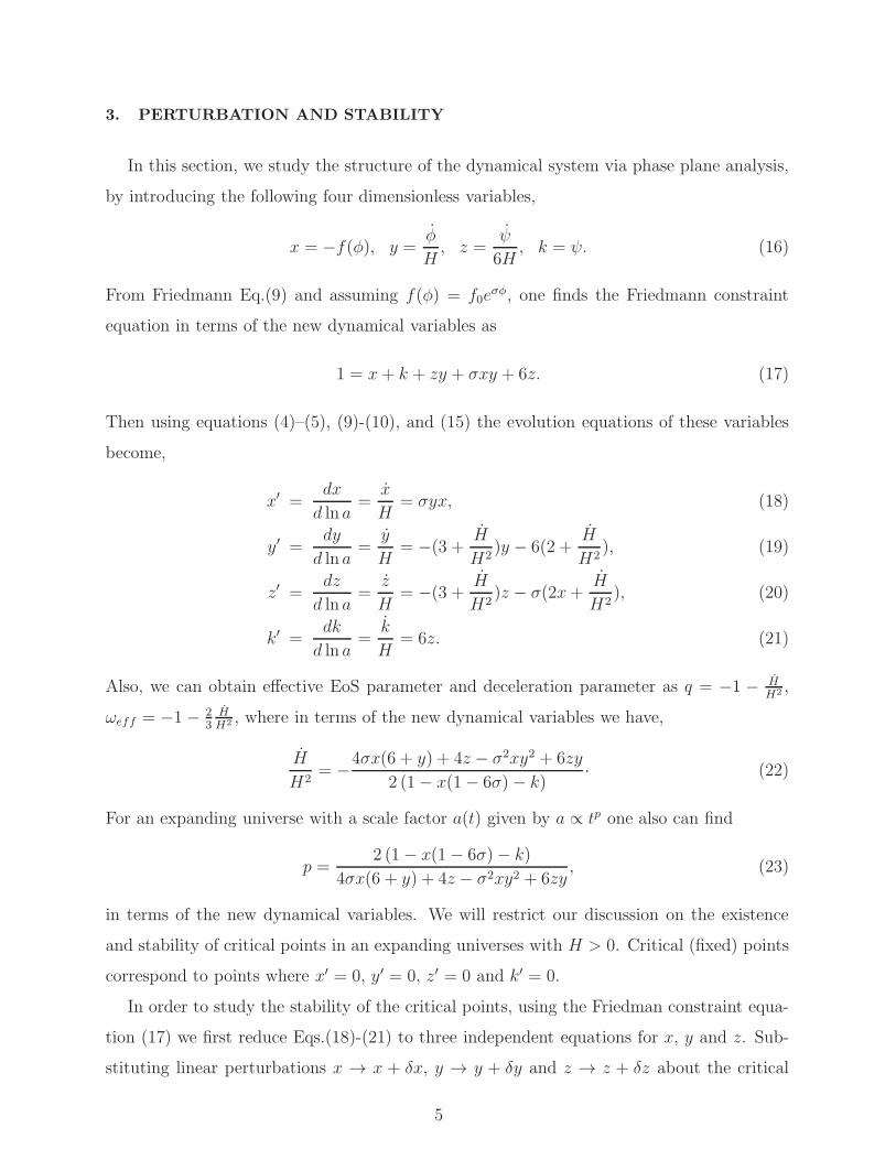
Label x y z ωeff q p Stability

S 1 0 0 1

31 1

2stable

TABLE I: The properties of the critical point.

The stable critical point, S, represents a scalar field-dominated solution in the radiation

dominated evolutive universe with a ∝ t1

2 . In Fig. 1, the attraction of trajectories to the

critical point in the three dimensional phase plane is shown for the given initial conditions.

6

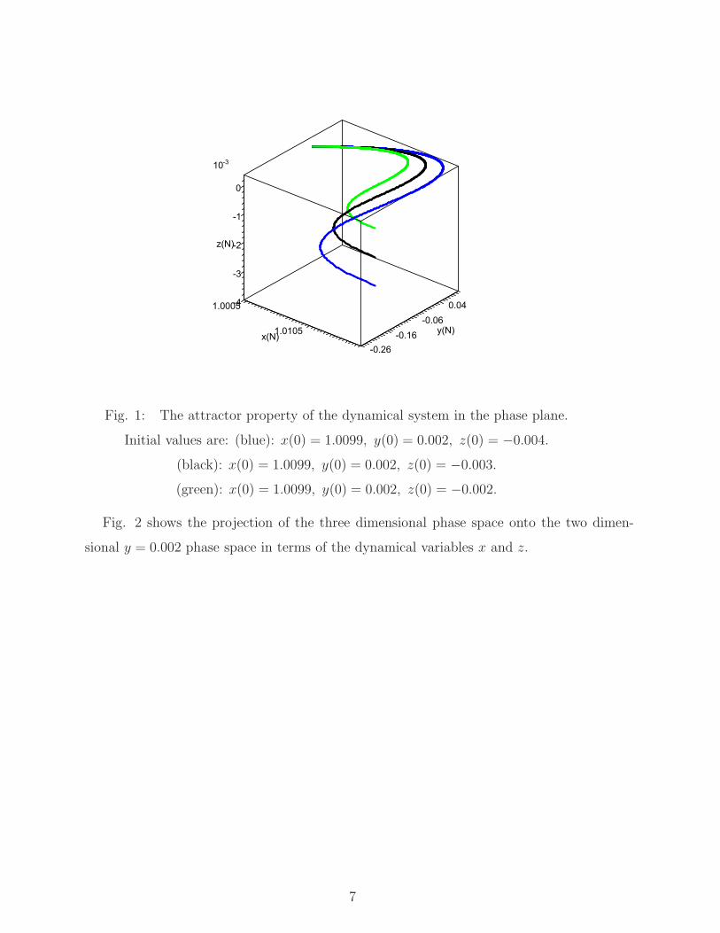
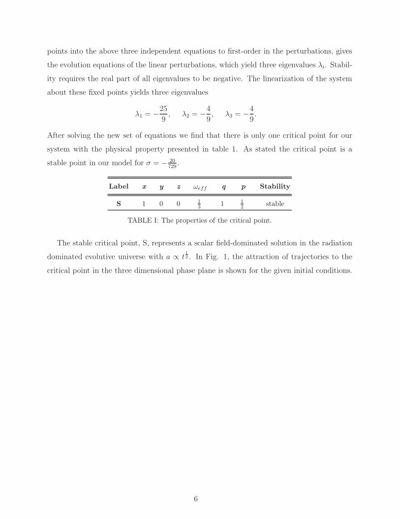
Fig. 1: The attractor property of the dynamical system in the phase plane.

Initial values are: (blue): x(0) = 1.0099, y(0) = 0.002, z(0) = −0.004.

(black): x(0) = 1.0099, y(0) = 0.002, z(0) = −0.003.

(green): x(0) = 1.0099, y(0) = 0.002, z(0) = −0.002.

Fig. 2 shows the projection of the three dimensional phase space onto the two dimen-

sional y = 0.002 phase space in terms of the dynamical variables x and z.

7

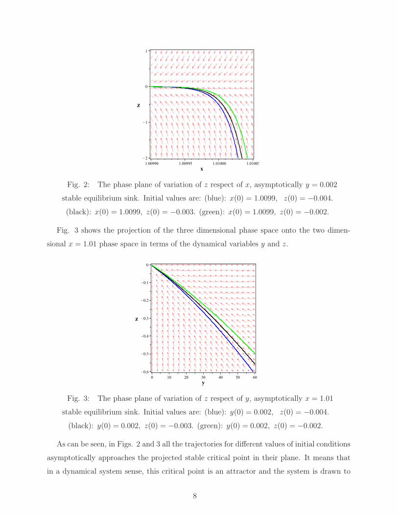
Fig. 2: The phase plane of variation of z respect of x, asymptotically y = 0.002

stable equilibrium sink. Initial values are: (blue): x(0) = 1.0099, z(0) = −0.004.

(black): x(0) = 1.0099, z(0) = −0.003. (green): x(0) = 1.0099, z(0) = −0.002.

Fig. 3 shows the projection of the three dimensional phase space onto the two dimen-

sional x = 1.01 phase space in terms of the dynamical variables y and z.

Fig. 3: The phase plane of variation of z respect of y, asymptotically x = 1.01

stable equilibrium sink. Initial values are: (blue): y(0) = 0.002, z(0) = −0.004.

(black): y(0) = 0.002, z(0) = −0.003. (green): y(0) = 0.002, z(0) = −0.002.

As can be seen, in Figs. 2 and 3 all the trajectories for different values of initial conditions

asymptotically approaches the projected stable critical point in their plane. It means that

in a dynamical system sense, this critical point is an attractor and the system is drawn to

8

this point in a self-organizing manner.

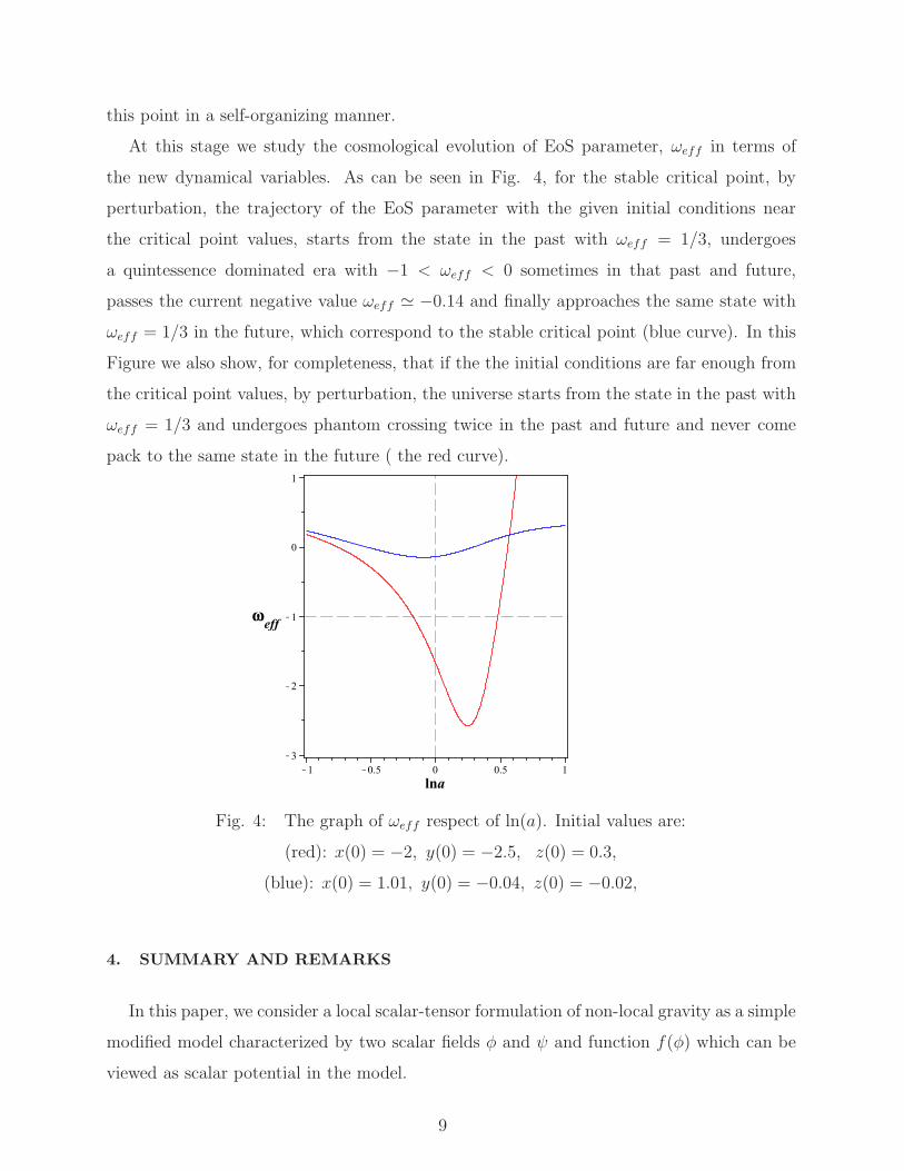
At this stage we study the cosmological evolution of EoS parameter, ωeff in terms of

the new dynamical variables. As can be seen in Fig. 4, for the stable critical point, by

perturbation, the trajectory of the EoS parameter with the given initial conditions near

the critical point values, starts from the state in the past with ωeff = 1/3, undergoes

a quintessence dominated era with −1 < ωeff < 0 sometimes in that past and future,

passes the current negative value ωeff ≃ −0.14 and finally approaches the same state with

ωeff = 1/3 in the future, which correspond to the stable critical point (blue curve). In this

Figure we also show, for completeness, that if the the initial conditions are far enough from

the critical point values, by perturbation, the universe starts from the state in the past with

ωeff = 1/3 and undergoes phantom crossing twice in the past and future and never come

pack to the same state in the future ( the red curve).

Fig. 4: The graph of ωeff respect of ln(a). Initial values are:

(red): x(0) = −2, y(0) = −2.5, z(0) = 0.3,

(blue): x(0) = 1.01, y(0) = −0.04, z(0) = −0.02,

4. SUMMARY AND REMARKS

In this paper, we consider a local scalar-tensor formulation of non-local gravity as a simple

modified model characterized by two scalar fields φ and ψ and function f(φ) which can be

viewed as scalar potential in the model.

9

We have made a perturbative analysis of the cosmological model, to investigate the

stability of the model. The perturbative equations of motion are solved numerically, and we

found that the system is stable for only one critical point under scalar perturbation. The

three dimensional phase space of the model gives the corresponding conditions for tracking

attractor. We have also shown the projected two dimensional phase space in x = constant

and y = constant planes. The stability analysis shows that, for the only stable critical point,

the phantom crossing never occurs. After perturbation, the universe approaches a stable

attractor in the future with ωeff = 1/3 (radiation dominated era) and p = 1/2 (decelerating

expansion era). The universe may undergoes phantom crossing if the chosen initial condition

are far enough from the critical point values, such that the universe never come back to the

initially stable state.

[1] A. G. Riess et al. Astrophys. J. 607 (2004) 665;

[2] C. L. Bennett et al., Astrophys. J. Suppl. 148 (2003) 1.

[3] K. Abazajian et al. Astron. J. 129 (2005) 1755; Astron. J. 128 (2004) 502; M. Tegmark et al.

Astrophys. J. 606 (2004) 702.

[4] S. W. Allen et al., Mon. Not. Roy. Astron. Soc. 353 (2004) 457.

[5] S. J. Perlmutter et al., Astrophys. J. 517 (1999) 565; A. G. Riess et al., Astron. J. 116 (1998)

1009;

[6] J. L. Tonry et al. Astrophys. J. 594 (2003) 1; M. Tegmark at al. Phys. Rev. D 69 (2004)

103501.

[7] P. Astier et al., Astron. Astrophys. 447 (2006) 31; A. G. Riess et al., Astrophys. J. 659

(2007)98; W. M. Wood- Vasey et al., Astrophys. J. 666 (2007) 694; M. Jamil, M. A. Rashid,

Eur.Phys.J.C60:141-147,(2009); M. Jamil, F. Rahaman, Eur. Phys. J. C 64 (2009) 97-105; M.

Jamil, Int.J.Theor.Phys.49:144-151,(2010); H. Farajollahi, N. Mohamadi, Int. J. Theor. Phys.,

49, 1, 72-78,(2010); M. Jamil, Int.J.Theor.Phys.49:62-71,(2010); H. Farajollahi, N. Mohamadi,

H. Amiri, Mod. Phy. lett. A, Vol. 25, No. 30 -2579-2589 (2010).

[8] D. N. Spergel et al. [WMAP Collaboration], Astrophys. J. Suppl. 148, 175 (2003); D. N.

Spergel et al., Astrophys. J. Suppl. 170 (2007) 377.

[9] D. J. Eisenstein et al. [SDSS Collaboration], Astrophys. J. 633 (2005) 560.

10

[10] U. Seljak at al. Phys. Rev. D 71 (2005) 103515; M. Tegmark, JCAP 0504 (2005) 001.

[11] R. R. Caldwell, Phys. Lett. B 545 (2002) 23;

[12] S. Nesseris, L. Perivolaropoulos, Phys. Rev. D 70 (2004) 123529;

[13] P. Singh, M. Sami, N. Dadhich, Phys. Rev. D68 (2003) 023522.

[14] Z.-K. Guo, Y.-Z. Zhang, Phys. Rev. D 71 (2005) 023501 ; S. M. Carroll, A. de Felice, M.

Trodden, Phys. Rev. D 71 (2005) 023525; I. Ya. Arefeva, A. S. Koshelev, S. Yu. Vernov,

Theor. Math. Phys. 148 (2006) 895;

[15] E. J. Copeland, M. Sami and S. Tsujikawa, Int. J. Mod. Phys. D 15 (2006) 1753.

[16] T. Chiba, T. Okabe and M. Yamaguchi, Phys. Rev. D 62 (2000) 023511; C. Armendariz-Picon,

V. Mukhanov and P. J. Steinhardt, Phys. Rev. Lett. 85 (2000) 4438.

[17] S. Capozziello, V. F. Cardone, S. Carloni and A. Troisi, Int. J. Mod. Phys. D 12 (2003) 1969;

S. M. Carroll, V. Duvvuri, M. Trodden and M. S. Turner, Phys. Rev. D 70 (2004) 043528; S.

Nojiri and S. D. Odintsov, Phys. Rev. D 68 (2003) 123512.

[18] M. R. Setare, Phys. Lett. B 654,(2007)1-6; M. R. Setare, Eur. Phys. J. C 52,(2007) 689; Y.

Piao and E. Zhou, Phys. Rev. D 68 (2003) 083515; M. R. Setare, Phys.Lett. B 642,(2006)1-4;

G. R. Dvali, G. Gabadadze and M. Porrati, Phys. Lett. B 485 (2000) 208; V. Sahni and Y.

Shtanov, JCAP 0311 (2003) 014;

[19] S. Tsujikawa, Phys. Rev. D 76 (2007) 023514, astro-ph/0705.1032v4

[20] S. Nojiri and S. D. Odintsov, Int. J. Geom. Meth. Mod. Phys. 4 (2007) 115; J. Phys. Conf.

Ser. 66 (2007) 012005, hep-th/0611071; J. Sadeghi, M.R. Setare, A. Banijamali and F. Milani,

Phys. Lett. B. 662 (2008) 92; S. Zhang and B. Chen, Phys. Lett. B. 669 (2008) 4; J. Sadeghi,

F. Milani and A. R. Amani, Mod. Phys. Lett. A 24, 29 (2009) 2363;

[21] H. Farajollahi, F. Milani, Mod. Phy. lett. A, Vol. 25, No. 27 (2010) 2349-2362.

[22] S. Nojiri, S. D. Odintsov, Phys. Rev. D 68 (2003) 123512; K. Bamba, C. Q. Geng, S. Nojiri

and S. D. Odintsov, Phys. Rev. D 79 (2009) 083014; K. Bamba, C. Q. Geng, S. Nojiri, JCAP

0810 (2008) 045;

[23] H. Farajollahi, A. Salehi, Int. J. Mod. Phys. D, Vol. 19, No. 5 (2010) 1-13

[24] J. Sadeghi, M. R. Setare, A. Banijamali and F. Milani, Phys. Rev. D. 79 (2009) 123003; M.

R. Setare, E. N. Saridakis, Phys.Lett.B670 (2008)1.

[25] F. Faraoni, Phys. Rev. D75 (2007) 067302; J. C. C. de Souza, V. Faraoni Class. Quant. Grav.

24 (2007) 3637; S. Nojiri, S. D. Odintsov, Phys. Rev. D 74 (2006) 086005; S. Capozziello, S.

11

Nojiri, S. D. Odintsov and A. Troisi, Phys. Lett. B 639 (2006) 135; S. Fay, S. Nesseris and

L. Perivolaropoulos, Phys. Rev. D 76 (2007) 063504; W. Hu and I. Sawicki, Phys. Rev. D 76

(2007) 064004; Y. Song, H. Peiris and W. Hu, Phys. Rev. D 76 (2007) 063517; S. Nojiri and

S. D. Odintsov, Phys. Lett. B 657 (2007) 238; Phys. Lett. B 652 (2007)343; S. A. Appleby

and R. A. Battye, Phys. Lett. B 654 (2007) 7.

[26] E. J. Copeland, S. Lee, J. E. Lidsey and S. Mizuno, Phys. Rev. D 71 (2005) 023526; Yi-Fu Cai,

E. N. Saridakis, M. R. Setare, Jun-Qing Xia, arXiv:0909.2776; E. N. Saridakis, S. V. Sushkov,

Phys.Rev.D81:083510,2010; E. N. Saridakis, J. Ward, Phys. Rev. D 80, 083003 (2009);

[27] S. Tsujikawa and M. Sami, Phys. Lett. B 603 (2004) 113; P. K. Townsend and M. N. R.

Wohlfarth, Class. Quant. Grav. 21 (2004) 5375; B. Boisseau, G. Esposito-Farese, D. Polarski,

A. A. Phys. Rev. Lett. 85 (2000) 2236; V. Sahni, Yu. V. Shtanov, JCAP 0311 (2003) 014;

Z.-K. Guo, Y.-S. Piao, X. Zhang, Y.-Z. Zhang, Phys. Lett. B 608 (2005) 177; M. Sami, A.

Toporensky, P. V. Tretjakov, Sh. Tsujikawa, Phys. Lett.

[28] M. R. Setare, E. N. Saridakis, JCAP0809:026,(2008) K. Nozari, M. R. Setare, T. Azizi and

N. Behrouz, Phys. Scripta 80 (2009) 025901; X. m. Chen, Y. Gong, E. N. Saridakis, JCAP

0904:001,(2009).

[29] S. Jhingan, S. Nojiri, S. D. Odintsov, M. Sami, I Thongkool, S. Zerbini, Phys. Lett. B

663,(2008)424. H. Farajollahi, A. Salehi, JCAP, 11, 006 (2010).

[30] S. Nojiri and S. D. Odintsov, Phys. Lett. B 659 (2008) 821.

12