1

Corporate Finance Review, Nov/Dec,7,3,13-21, 2002

The Jackknife Estimator for Estimating Volatility of Volatility of a Stock

Hemantha S. B. Herath* and Pranesh Kumar**

*Assistant Professor, Business Program, University of Northern British Columbia, 3333 University Way, Prince George, British Columbia, Canada V2N 4Z9; Tel (250) 960-6459; email: herathh@unbc.ca. ** Associate Professor, Mathematics and Computer Science, University of Northern British Columbia, 3333 University Way, Prince George, British Columbia, Canada V2N 4Z9; Tel (250) 960-6671; email: kumarp@unbc.ca.

2

Abstract

In this paper we demonstrate application of a statistical technique to estimate the

volatility of volatility of a stock, based on re-sampling method. The jackknife technique

is easy to implement, useful in case of small sample data and does not place a heavy

burden on data requirements. The paper describes the jackknife procedure and illustrates

how it can be used to estimate the volatility of volatility. To demonstrate its practical use

the pricing bias is analyzed using the stochastic volatility estimate as input in Hull and

White (1987) model. Finally, confidence intervals are constructed for selecting among

different weighting schemes as summarized in Mayhew (1995). The proposed technique

is ideal for small data sets when implementing stochastic option pricing models.

3

The Jackknife Estimator for Estimating Volatility of Volatility of a Stock

Introduction

The Black-Scholes option-pricing model for valuing a European option on a

dividend-protected stock depends upon five parameters, the stock price (S), exercise price

(K), volatility of the stock (σ), time to maturity (T) and the risk-free rate (r). The value

of a call option (C) can be written as

)(N)(N 21 dKedSC rT−−=

where T

TrTSdσ

σ )2()log( 2

1++

= and . 12 Tdd σ−=

and N(d) is the cumulative normal distribution value evaluated at d.

Except for the volatility of the stock, all of the other parameters of the model are

relatively easy to observe. The historic volatility of the stock can be estimated by

computing the standard deviation of continuous price return of a series of recent stock

prices. Along with the other parameters, the historic volatility can be plugged into the

Black-Scholes formula to derive a price for the option. As an alternative, the stock's

volatility can be inferred from the market price of a stock by inverting the Black-Scholes

formula. This procedure involves substituting the option's market price along with

values for the exercise price, the time to maturity, risk free rate and the initial stock price

in the model and solving for the volatility parameter. The volatility parameter based on

the market price of an option is called the implied volatility.

The Black and Scholes (BS) formula depends on 10 unrealistic assumptions but

the formula works well than any other formula in a wide range of circumstances (Black

1993). Among others, a critical assumption of the BS model is that a stock's volatility is

4

known and doesn't change over the life of the option. Contrary to this assumption,

empirical evidence on stock prices and their derivatives strongly suggest that the

volatility of a stock is not constant. The asset price volatility is indeed stochastic.

Consequently, changes in the volatility of a stock may have a major impact on the value

of an option, especially if the option is far out-of-the money.

Since the development of the path breaking BS (1973) model, many researchers

have tried to relax its most stringent assumptions. Researchers have introduced

stochastic volatility models that relax the constant volatility assumption. When asset

prices do not exhibit continuous processes, and researchers have introduced jump

diffusion models Merton (1976), Cox and Ross (1976). Many researchers including

Scott (1987, 1991), Hull and White (1987, 1988), Heston (1993a and 1993b) have

generalized the BS model to incorporate stochastic volatility. In order to implement

stochastic option pricing models, an input parameter, the volatility of volatility of the

asset has to be estimated. Ball and Roma (1994), state that estimation problems in

implementing stochastic volatility models are a promising area for future research.

The following quote from Black's (1993) article and above observation by Ball

and Roma (1994) motivated our research: '' Since the volatility can change, we should

really include ways in which it can change the formula. The option value will depend on

the entire future path that we expect the volatility to take, and on the uncertainty about

what the volatility will be at each point in the future. One measure of that volatility is the

volatility of volatility''. The basic question that leads from the above is: how can one

measure a stock's volatility of volatility? Also, if the volatility of an underlying asset

5

itself is stochastic, as assumed in stochastic volatility models, from an implementation

point of view, it is important to estimate the volatility of volatility.

Hull and White (1987) suggest two alternative methods to estimate the volatility

of volatility, which is a parameter in their stochastic option model. They compare each

of the two methods. First, the volatility of volatility is estimated by examining the

changes in volatility implied by option prices. Using the implied volatility is an indirect

procedure and the results they argue can be contaminated since the changes in implied

volatility to some extent can be attributed to pricing errors in the options. Alternatively,

they suggest that one could use the changes in estimates of the actual variances to

estimate the volatility of volatility. This however, would require very large amounts of

data.

In this paper, we propose yet another statistical method to estimate the volatility

of volatility based on re-sampling techniques. The jackknife re-sampling technique is

easy to implement and does not place a heavy burden on data requirements. The

jackknife is a versatile statistical procedure based on the principle of replicability for

estimating the standard error of a statistic non-parametrically. We demonstrate the

usefulness of the jackknife procedure in estimating the volatility of volatility of a stock.

Although the procedure is simple to apply there is a general lack of its use in option

pricing applications. The proposed technique is ideal for small data sets when

implementing stochastic option pricing models.

The paper is organized as follows. First, we describe the jackknife procedure in

detail. Second, we illustrate the jackknife procedure using an example from Gemmill

(1992). Weighted-average techniques for computing the implied volatility have received

6

quite a bit of attention. However, there are mixed results as to whether implied volatility

is better at forecasting future volatility than estimators based on historic data. Next, we

use the jackknife estimate of stochastic volatility as input in Hull and White (1987)

stochastic volatility model to illustrate the pricing bias. Finally, in order to select

volatility estimates based on statistical comparison of different weighting schemes, we

use the jackknife volatility of volatility estimates to construct confidence intervals for

different weighting schemes as summarized in Mayhew (1995).

Jackknife procedure

The jackknife method is computationally intensive but is easy to use

especially if the sample size is small. Efron and Gong (1983) discuss properties of the

jackknife and compare it with the bootstrap method. Buzas (1997) provides an approach

that is faster for estimating the jackknife standard error. The jackknife procedure has

several advantages over other methods. First, it is appropriate for small samples such as

the weekly two-year stock price data typically used for estimating the historic volatility

of a stock. Second, the procedure is sensitive enough to detect the influence of outliers

on the analysis. Third, it uses all the data while eliminating potential bias related to the

inclusion of atypical data. Finally, as we will demonstrate it can easily be implemented

on a spreadsheet and does not need special statistical packages or computer programs as

required for the bootstrap method.

Let R1, R2, ……,Rn be the percent returns for a stock over the n trading periods

calculated from the sequence of the successive closing prices for that stock, i.e., the

percent return

7

⎥⎦

⎤⎢⎣

⎡ +=

−1

log100t

ttt price

dividendspriceR

The standard deviation of the returns σ is a commonly used measure of the volatility of a

stock. In order calculate the price on a European call using the Black and Scholes model

the estimate of the historic volatility 21

)(1

1 RRn

n

t t −−= ∑ =

σ can be used where the

mean return ∑ ==

n

t tRn

R1

1 is based on the n returns.

In order to implement stochastic option pricing models, we need to measure the

volatility of the volatility of a stock, say psi (ξ ). We argue that the jackknife technique

can be efficiently employed to estimate ξ, using the same returns data used to find a

stock’s volatility σ. The procedure is as follows. A given sample n is partitioned into m

sub-samples all of which must be the same size. The value of m can range between one

and the largest multiplicative factor of n. We first calculate a pseudovalue in ,1−θ , which

is the standard deviation of returns after each observation is omitted. We repeat

computation of pseudovalues based on sub-samples to obtain the jackknife estimate of

the volatility of the volatility. Notice that the jackknife statistic is based on the (n – 1)

returns excluding Ri for the ith sub-sample. For example, if there are 19 observations for

stock returns in the sample, to generate the first pseudovalue, the first observation is

omitted and the statistic computed from the remaining 18 observations: to generate the

second sub-sample the second observation is omitted from the given sample of 19

observations. This procedure is repeated until 19 pseudovalues are computed. Then

following Tukey (1958), we estimate the volatility of volatility ξ, by

8

21

1,1 )(1ˆ

−=

− −−

= ∑ n

n

iinn

n θθξ

where ∑ = −− =n

i inn n1 ,11 θθ .

An Example

We illustrate the jackknife procedure using an example from Gemmill (1992).

We selected the same data that Gemmill (1986) used to analyze different volatility

weighting schemes and implied volatility. In Table 1, 20 end of week prices and

dividends for the British oil company, BP for the period August 23 to January 3, 1992 are

presented. The return for week 2 in Table 1 is computed as R2 = 100[ln (352.5/347)] =

1.5726. The average return of the stock price is -0.8452 per week and standard deviation

is (σw = 3.0363%) per week. The annual historic volatility of BP stock is calculated as

22%. The historic volatility of 22% could then be used in the Black and Scholes model

as a forecast of future volatility.

Next, by applying the jackknife procedure we estimate the volatility of volatility

of BP stock as ξ = 3.26%. The Microsoft Excel formulas for computing the average

returns, volatility, pseudovalues and the volatility of volatility are presented in Table 1.

The jackknife procedure is computationally efficient, since the same 20 end of week

prices that are used to estimate the historic volatility can be used to estimate the volatility

of volatility. It requires less data unlike the estimation procedures of Hull and White that

uses changes in estimates of the actual variances. Furthermore, it is also easy to

implement unlike bootstrap procedures. These advantages make it a good choice as an

estimation procedure for implementing stochastic volatility models. In the next section,

9

we use the stochastic volatility parameter that we estimated using the jackknife technique

to illustrate the pricing bias of a BP call option.

[Insert Table 1 Here]

Pricing Bias of BP Calls Caused by Stochastic Volatility

In order to illustrate the pricing bias due to stochastic volatility, we use BP call

option data from Gemmill (1992). A series of BP calls with an initial stock price S = 291,

volatility σ = 22%, days to maturity (T ) = 19 for January call, 110 for April call and 201

for July has the market prices as shown in Table 2. The risk free rate is r = 11% or

(0.1044 compounded continuously). The BS prices based upon the historic volatility of

22% are given in brackets in Table 2.

[Insert Table 2 Here]

In order to demonstrate the pricing bias we use the stochastic volatility parameter

ξ = 3.26% estimated for BP stock using the jackknife procedure as an input in the Hull

and White (1987) stochastic volatility model. Hull and White (1987) developed a model

to price a European call on an asset with stochastic volatility. The option price is

determined in series form for the case where the stochastic volatility is independent of its

underlying stock price. The series form of Hull and White model with the first three

terms of the series solution is given below.

⎥⎦

⎤⎢⎣

⎡−

−−−′+−= − 4

2

4

3211

212 )1(2

4)1)((N

21)(N)(N),( σσ

σσ

kkedddTSdKedSSf

krT

10

5

22

2121211

8)()1)(3)((N

61

σdddddddTS +−−−′

+

.....,3

)618248()189(3

3236 +⎥

⎦

⎤⎢⎣

⎡ +++++−×

kkkkeke kk

σ

where, k = ξ2T , T

TrTSdσ

σ )2()log( 2

1++

= and . 12 Tdd σ−=

In order to compare the pricing bias, of the Hull and White and BS models we use

the at-the-money April 300 call which has just over three months to maturity. The April

300 call is treated as the marker since it is nearest to the money. The implied volatility is

16% since, by setting σ = 16% we obtain a BS price of 10 which is exactly equal to the

market price. The call option parameters to determine the pricing bias are σ = 16%, ξ =

3.26%, T = 110 days, and r = 10.44% respectively. In Figure 1, we compare the Hull

and White call prices with the BS model. In order to illustrate the pricing bias, we have

exaggerated the bias 25,000 times since the actual pricing error is quite small. When the

volatility is un-correlated with the stock we find that the Hull and White option price is

lower compared to the BS price for near the money options. The BS price is too low for

deep in the money and deep out of the money and high at the money. These observations

are consistent with the Hull and White (1987) findings.

[Insert Figure 1 Here]

Confidence Intervals for Weighted Average Implied Volatility

Weighted-average techniques for computing the implied volatility have received

quite a bit of attention. For prices of multiple options with varying strike prices and

11

maturity written on the same underlying asset implied volatility are not the same. For

instance, for the six BP call options in Table 1 the implied volatility are found to be Jan-

280 (15%), Apr-280 (8%), July-280 (1%), Jan –300 (22%), Apr-300 (16%) and July-300

(14%). Consequently, researches have developed various weighting schemes to derive a

single implied volatility estimate that can be used to price options. Mayhew (1995)

provide an excellent literature review on option–implied volatility. In his article, he

describes four implied volatility-weighting schemes that range from simple equal weights

to more complex elasticity weighting.

An important issue in volatility is its predictive ability. Among others, early

literature such as, Latene and Rendleman (1976), Schmalensee and Trippi (1978) and

Beckers (1981) found that implied volatility is better than historic volatility at predicting

actual volatility. Gemmill (1986) compared historic volatility and six different implied

volatility schemes- equal weights, elasticity weights, minimized squared pricing errors,

at-the-money implied volatility, out-of-the money implied volatility, in the money

implied volatility to ascertain the predictive ability of actual volatility. By regressing the

predictors on the actual volatility, Gemmill found that at-the-money implied volatility is

the best predictor of future volatility. Subsequent literatures also support this claim but

results have been mixed Mayhew (1995).

In this section, we use the volatility of volatility estimate obtained using the

jackknife technique to construct confidence intervals for historic volatility (Historic) and

four volatility schemes described in Mayhew (1995) to identify the best predictor of

actual volatility. The four weighted average implied volatility measures are:

(1) Equal weights used by Schmalensee and Trippi (1978) - (Equal weighting);

12

(2) Black-Scholes Vega weighting scheme of Latene and Rendleman (1976) –(Vega

Weighting);

(3) Volatility elasticity used by Chiras and Manaster (1978) – (Elasticity Weighting);

(4) Beckers (1981) Implied Standard Deviation – (Beckers ISD).

The different weighting schemes along with the parameter description and the

volatility estimates are summarized in Table 3. The volatility based on the four

weighting schemes range from 8.3% to 18.5%. Of the four weighting schemes, Beckers

ISD provide the volatility estimate closest to the implied volatility (16%) of the April

300-marker call option.

[Insert Table 3 Here]

Next, using the volatility of volatility estimates obtained from the Jackknife

procedure we develop the 95% and 99% confidence intervals for each of the weighted

average implied volatility scheme. The confidence intervals for historic and the four

weighted average volatility are presented in Figure 2. In Table 4, we present the

estimated call values for the six BP call options. The call prices indicate that for near-

the-money options (300-Jan, 300-April and 300-July) historic volatility, elasticity

weighted and Beckers ISD perform better than the other weighting schemes. Vega

weighting of Chiras and Manaster (1978) price the in-the-money options better than the

other methods. The shaded regions in Table 4 show the best weighting schemes for near-

the-money and in-the-money options.

13

The confidence intervals for the call prices using the jackknife-based volatility of

volatility parameter are given in Table 5. Based on a 95% confidence interval for

implied volatility, we find that Vega weight is more appropriate compared to the other

weighting schemes for in-the money options. In case of pricing near-the-money options

the results are mixed. However, Beckers ISD is found to be consistently performing

better for all three near-the money options followed by historic volatility and elasticity

weighted scheme as shown by the shaded regions in Table 5.

[Insert Figure 2 Here]

[Insert Table 4 Here]

[Insert Table 5 Here]

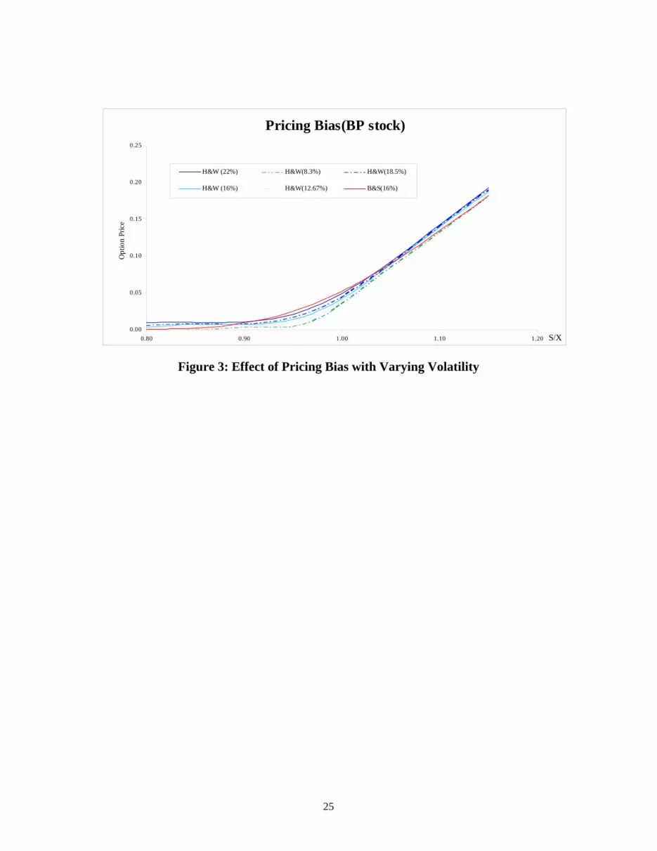
Next, we study the pricing bias of Hull and White stochastic volatility model and

the BS model when different weighted volatility values are used. According to Hull and

White (1987) the principle result of increasing volatility is to make the bias more positive

for out-of-the options and more negative for in-the money options. Consistent with their

findings, the pricing bias is minimum when Hull and White model with historic volatility

of 22% is compared to the BS with implied volatility of 16%. The pricing bias of BS is

maximum when Vega weighting of 8.3% is used in the Hull and White stochastic

volatility model. As shown in Figure 3 the graphs indicate that the bias is inversely

related with the volatility of the stock.

14

[Insert Figure 3 Here]

Conclusions

In this paper we introduce a relatively easy and efficient statistical approach to estimating

the volatility of volatility of an asset. A key contribution of this paper is the Jackknife

procedure to empirically estimate the volatility of volatility parameter, which is an input

to stochastic volatility models. The jackknife method is easy to use especially if the

sample size is small such as the weekly two-year stock price data typically used for

estimating the volatility of a stock. It can easily be implemented on a spreadsheet and

does not need special statistical packages or computer programs. It provides more

conservative and less biased volatility of volatility estimates for implementing stochastic

option pricing models. Further since the purpose of deriving prediction models is for

prediction with future samples, and if a model does not predict well with future samples,

the purpose for which model is designed is lost. Thus, when an external replication is not

feasible, the jackknife statistic is the most appropriate technique to determine result

stability [Ang(1998)].

Next, we demonstrated how one could use volatility of volatility estimates to

develop confidence intervals for selecting among different weighting schemes. As future

extension of this research, we plan to perform a comparative study of different replication

techniques to estimate the volatility of volatility of a stock.

15

References

Ang, R. P. 1998. "Use of the Jackknife Statistic to Evaluate Result Replicability."

Journal of General Psychology, 125(3), 218-228.

Ball C. A., and A. Roma. 1994. “Stochastic Volatility Option Pricing.” Journal of

Financial and Quantitative Analysis, vol. 29: 589-607.

Beckers S. 1981. “Standard Deviation Implied in Option Prices as Predictors of Future

Stock Price Variability.” Journal of Banking and Finance, vol. 5, no. 3,

(September): 363-82.

Black F. 1993. “How to Use the Holes in Black Scholes.” In The New Corporate

Finance: Where Theory Meets Practice, ed. by D. H. Chew, McGraw-Hill:

419-425

Black F., and M. Scholes. 1973. “The Pricing of Options and Corporate Liabilities.”

Journal of Political Economy, vol. 81, no. 3, (May/June): 673-659

Briys E., M. Bellalah, M. H. Mai, F. De Varenne. 1998. Options Futures and Exotic

Derivatives: Theory, Application and Practice, John Wiley and Sons.

Buzas, J.S. 1997. “Fast Estimators of the Jackknife.” The American Statistician, vol. 51,

no.3: 235-240.

Chance D. M. 1999. “Research Trends in Derivatives and Risk Management since

Black-Scholes.” Journal of Portfolio Management, May: 35-46.

Chiras D. P., and S. Manaster. 1978. “The Information Content of Option Prices and a

Test of Market Efficiency.” Journal of Financial Economics, vol. 6, nos. 2/3,

(June/September): 213-234

16

Cox J. C., and S. A. Ross. 1976. “The Valuation of Options for Alternative Stochastic

Processes.” Journal of Financial Economics, vol. 3: 146-166

Efron, B, and G. Gong. 1983. “A Leisurely Look at the Bootstrap, the Jackknife and

Cross Validation.” The American Statistician, vol. 37: 36-48.

Gemmill G. 1986. “The Forecasting Performance of Stock Options on the London

Traded Options Market.” Journal of Business Finance and Accounting, vol. 13,

No. 4 (Winter): 535-46.

Gemmill G. 1992. Options Pricing- An International Perspective, McGraw-Hill.

Heston S. 1993 (a). “A Closed Form Solution for Options with Stochastic Volatility with

Application to Bond and Currency Options.” Review of Financial Studies, vol. 6:

327-343.

Heston S. 1993 (b). “Invisible Parameters in Option Pricing.” Journal of Finance, vol.

48, no. 3: 933-947.

Hull J. and A. White. 1987. “The Pricing of Options on Assets with Stochastic

Volatilities.” Journal of Finance, vol. 42, no. 2 (June): 281-300.

Hull J. and A. White. 1988. “An Analysis of the Bias in Option Pricing Caused by a

Stochastic Volatility.” Advances in Futures and Options Research, vol. 3: 29-61.

Latane H. A., and R. J. Rendleman Jr. 1976. “Standard Deviations of Stock Price Ratios

Implied in Option Prices.” Journal of Finance, vol. 31, no. 2, (May): 369-381.

Mayhew S. 1995. “Implied Volatility.” Financial Analyst Journal, 51, July-August: 8-20.

Merton R. C. 1976. “Option Pricing when Underlying Stock Returns are Discontinuous.”

Journal of Financial Economics, vol. 3, (January-March): 125-144.

17

Schmanlensee R., and R. Trippi. 1978. “Common Stock Volatility Expectations Implied

by Option Premia.” Journal of Finance, vol. 33, no. 1, (March):129-147.

Scott L. O. 1987. “Option Pricing when the Variance Changes Randomly.” Journal of

Financial and Quantitative Analysis, vol. 22: 419-438.

Scott L. O. 1991. “Random Variance Option Pricing: Empirical Tests of the Model and

Delta-Sigma Hedging.” Advances in Futures and Options Research,

vol. 5: 113-135.

Tukey, J.W. 1958. “Bias and Confidence in Not-Quite Large Samples.” (Abstract).

Ann. Math. Statistics, vol. 28: 362.

18

TABLE 1

Weekly Prices Returns and Jack-knife Estimates for BP Stock (August – January 1992)

Week Price Return (ri)Standard Deviation

of ri ( θ18)Cell A B C

1 347

2 352.5 1.5726 3.0657

3 346 -1.8612 3.1140

4 337 -2.6356 3.0923

5 331 -1.7965 3.1153

6 336.5 1.6480 3.0619

7 339 0.7402 3.0992

8 341 0.5882 3.1038

9 352 3.1749 2.9594

10 331 -6.1513 2.8307

11 328 -0.9105 3.1243

12 332.5 1.3626 3.0755

13 324 -0.8760 3.1243

14 311 -4.0951 3.0175

15 302 -2.9366 3.0805

16 291 -3.7104 3.0416

17 297.5 2.2091 3.0302

18 279 -6.4202 2.7985

19 277 -0.7194 3.1241

20 290.5 4.7586 2.7949

⎥⎦⎤

⎢⎣⎡=

3475.352ln100tR

8452.0B20):AVERAGE(B2 −==wR

0363.3B20):STDEV(B2 ==wσ

B20):STDEV(B3 )1,18( =θ

B20):B4STDEV(B2, )2,18( =θ

0344.319

C20):SUM(C2 18 ==θ

19

TABLE 2

Market and BS Model Prices for BP on 3 January 1992

January April July

Expiry price Market

price BS

price Market price

BS price

Market price

BS price

280 13 (14) 20 (26) 26 (34)

300 3 (3) 10 (14) 16 (23)

20

TABLE 3

Weighted Average Volatility

Description Model Estimated Volatility

Historic - 22%

Schmalensee and Trippi (1978) – (Equal weighting)

∑=

=N

iiN 1

1ˆ σσ

σi: implied volatility of ith call 12.67%

Latene and Rendleman (1976) (Vega Weighting)

∑∑ =

=

=N

iiiN

ii

ww 1

22

1

1ˆ σσ

wi: Black-Scholes vegas of option i

8.30%

Chiras and Manaster (1978) (Elasticity Weighting) ∑

∑

=

== N

i i

i

i

i

N

i i

i

i

ii

CC

CC

1

1ˆσ

δσδ

σδσδσ

σ

Ci: Market price of option i

18.5%

Beckers (1981) (Beckers ISD)

Minimize [ ]21

)ˆ(σii

N

ii BSCw −∑

=

BSi: Black-Scholes price of option i 16%

21

TABLE 4

Call Prices Based on Weighting Schemes

Call Option

Market Price Historic Equal

Weighting Vega

Weighting Elasticity Weighting

Beckers ISD

280-Jan 13 14 13 13 13 13

280-April 20 26 21 20 24 23

280-July 26 34 29 27 32 31

300-Jan 3 3 1 0 2 2

300-April 10 14 8 5 12 10

300-July 23 23 15 12 20 18

22

TABLE 5

Estimates of Call Prices Based on Confidence Intervals (CI) for Implied Volatility

Historic Equal Weighting Vega Weighting Elasticity Weighting Beckers ISD Call Option

Market Price

95% CI 99%CI 95% CI 99%CI 95% CI 99%CI 95% CI 99%CI 95% CI 99%CI

280-Jan 13 13.0 15.2 12.7 15.9 12.5 13.5 12.5 14.1 12.5 13.0 0.0 13.4 12.7 14.6 12.5 15.2 12.6 14.1 12.5 14.7

280-April 20 22.4 29.0 21.1 30.9 19.7 24.2 19.7 25.8 19.7 22.1 0.0 23.6 21.0 27.2 20.1 29.0 20.3 25.9 19.7 27.6

280-July 26 30.2 39.0 28.5 41.4 26.7 32.5 26.6 34.7 26.6 29.8 0.0 31.8 28.4 36.6 27.2 38.9 27.4 34.8 26.7 37.1

300-Jan 3 1.4 4.5 0.8 5.3 0.1 2.3 0.0 3.0 0.0 1.3 0.0 2.0 0.8 3.7 0.3 4.5 0.4 3.1 0.1 3.8

300-April 10 9.9 18.2 7.9 20.3 4.1 12.4 2.0 14.4 1.3 9.6 0.0 11.6 7.8 16.1 5.7 18.2 6.2 14.5 4.1 16.6

300-July 23 17.3 28.2 14.6 30.9 10.0 20.5 8.1 23.2 7.8 16.8 0.0 19.5 14.6 25.4 12.0 28.1 12.5 23.2 10.1 26.0

23

Figure 1: Pricing Bias when σ = 16%, ξ = 3.26%, T = 110 days, r = 10.44

Pricing Bias(BP stock)

0

5

10

15

20

25

30

35

40

45

0.80 0.90 1.00 1.10 1.20

S/X

Opt

ion

Pric

e

BS Model H&W model

24

1 Historic, 2 Equal Weighting, 3 Vega Weighting, 4 Elasticity Weighting, 5 Beckers ISD

Figure 2: Confidence Intervals for Historic and Weighted Average Volatility

Schemes.

Comparision o f Volatility Ranges Under Different Weighting Scheme

12%

3%

0%

9%

6%

15%

6%

2%

12%

9%

28%

19%

15%

25%

23%

32%

22%

18%

28%

26%

0%

5%

10%

15%

20%

25%

30%

35%

1 2 3 4 5

Vol

atili

ty

25

Figure 3: Effect of pricing bias with varying volatility.

Figure 3: Effect of Pricing Bias with Varying Volatility

Pricing Bias(BP stock)

0.00

0.05

0.10

0.15

0.20

0.25

0.80 0.90 1.00 1.10 1.20 S/X

Opt

ion

Pric

e

H&W (22%) H&W(8.3%) H&W(18.5%)

H&W (16%) H&W(12.67%) B&S(16%)