arX

iv:m

ath/

9902

025v

2 [

mat

h.O

C]

2 J

ul 1

999

Notions of Input to Output Stability

Eduardo Sontag∗

Dept. of MathematicsRutgers University

New Brunswick, NJ 08903sontag@control.rutgers.edu

Yuan Wang†

Dept. of MathematicsFlorida Atlantic University

Boca Raton, FL 33431ywang@math.fau.edu

Abstract

This paper deals with concepts of output stability. Inspired in part by regulator theory,several variants are considered, which differ from each other in the requirements imposedupon transient behavior. The main results provide a comparison among the various notions,all of which specialize to input to state stability (iss) when the output equals the completestate.

Keywords. input/output stability, ISS, nonlinear control, robust stability, partial stability, regulation

1 Introduction

This paper addresses questions of output stability for general finite-dimensional control systems

x(t) = f(x(t), u(t)), y(t) = h(x(t)) . (1)

(Technical assumptions on f , h, and admissible inputs, are described later.) Roughly, a sys-tem (1) is “output stable” if, for any initial state, the output y(t) converges to zero as t → ∞.Inputs u may influence this stability in different ways; for instance, one may ask that y(t) → 0only for those inputs for which u(t) → 0, or just that y remains bounded whenever u is bounded.Such behavior is of central interest in control theory. As an illustration, we will review belowhow regulation problems can be cast in these terms, letting y(t) represent a quantity such as atracking error. Another motivation for studying output stability arises in classical differentialequations: “partial” asymptotic stability (cf. [26]) is nothing but the particular case of ourstudy in which there are no inputs u and the coordinates of y are a subset of the coordinates ofx (that is to say, h is a projection on a subspace of the state space R

n). The notion of outputstability is also related to that of “stability with respect to two measures”, cf. [9].

The main starting point for our work is the observation that there are many different waysof making mathematically precise what one means by “y(t) → 0 for every initial state” (and,when there are inputs, “provided that u(t) → 0”). These different definitions need not resultin equivalent notions; one must decide how uniform is the rate of convergence of y(t) to zero,and precisely how the magnitudes of inputs and initial states affect convergence.

Indeed, our previous work on input-to-state stability (iss, for short) was motivated in muchthe same way. The concept of iss was originally introduced in [16] to address the problem wheny = x. Major theoretical results were developed in [19] and [22], and applications to controldesign can be found in, among others, [4], [6], [7], [8], [12], [15], [22], and [25], as well as in therecent work [13] as a foundation for the formulation of robust tracking.

Actually, the original paper [16] had already introduced a notion of input/output stability(ios), but the theoretical effort until now was almost exclusively directed towards the iss special

∗This research was supported in part by US Air Force Grant F49620-98-1-0242†This research was supported in part by NSF Grant DMS-9457826

1

case. (There are two ways to formulate the property of input/output stability and its variants.One is in purely input/output terms, where one uses past inputs in order to represent initialconditions. Another is in state space terms, where the effect of past inputs is summarized by aninitial state. In [16] an i/o approach was used, but here, because of our interest in initial-statedependence, we adopt the latter point of view. The relations between both approaches areexplained in [16] and in more detail in [10] and [5].)

It turns out that the ios case is substantially more complicated than iss, in the sense thatthere are subtle possible differences in definitions. One of the main objectives of this paper is toelaborate on these differences and to compare the various definitions; the companion paper [24]provides Lyapunov-theoretic characterizations of each of them.

A second objective is to prove a theorem on output redefinition which (a) extends one ofthe main steps in linear regulation theory to general nonlinear systems, and (b) provides oneof the main technical tools needed for the construction of Lyapunov functions in [24].

The organization of this paper is as follows. Section 1.1 starts with the review of certainfacts from regulation theory; this material is provided merely as an additional motivation forour study, and is not required in order to follow the paper. Because of the technical characterof the paper, it seems appropriate to provide an intuitive overview; thus, the rest of that sectiondescribes the main results in very informal terms. After that, in Section 2, we define our notionscarefully and state precisely the main results. The rest of the paper contains the proofs. Apreliminary version of this paper appeared in [23].

1.1 Additional Motivation and Informal Discussion

Output regulation problems encompass the main typical control objectives, namely, the analysisof feedback systems with the following property: for each exogenous signal d(·) (which mightrepresent a disturbance to be rejected, or a signal to be tracked), the output y(·) (respectively,a quantity being stabilized, or the difference between a certain variable in the system and itsdesired target value) must decay to zero as t → ∞. Typically (see e.g. [18], Section 8.2, or [14],Chapter 15 for linear systems, and [3], Chapter 8, for nonlinear generalizations), the exogenoussignal is unknown but is constrained to lie in a certain prescribed class (for example, the class ofall constant signals). Moreover, this class can be characterized through an “exosystem” givenby differential equations (for example, the constant signals are precisely the possible solutionsof d = 0, for different initial conditions).

In order to focus on the questions of interest for this paper, we assume that we alreadyhave a closed-loop system exhibiting the desired regulation properties, ignoring the question ofhow an appropriate feedback system has been designed. Moreover, let us, for this introduction,restrict ourselves to linear time-invariant systems (local aspects of the theory can be generalizedto certain nonlinear situations employing tools from center manifold theory, see [3]). The objectof study becomes:

z = Az + Pw

w = Sw

y = Cz + Qw ,

seen as a system x = f(x), y = h(x), where the extended state x consists of z and w; thez-subsystem incorporates both the state of the system being regulated (the plant) and thestate of the controller, and the equation w = Sw describes the exosystem that generates the

2

disturbance or tracking signals of interest. This is a system without inputs; later we explainhow inputs may be introduced into the model as well.

As an illustration, take the stabilization of the position y of a second order system y − y =u + w under the action of all possible constant disturbances w. The conventional proportional-integral-derivative (PID) controller uses a feedback law u(t) = c1q(t) + c2y(t) + c3v(t), forappropriate gains c1, c2, c3, where q =

∫y and v = y. Let us take c1 = −1, c2 = c3 = −2. If we

view the disturbances as produced by the “exosystem” w = 0, the complete system becomes

q = y , y = v , v = −q − y − 2v + w , w = 0

with output y. That is, the plant/controller state z is col (q, y, v), and

S = Q = 0 , A =

0 1 00 0 1−1 −1 −2

, C = (0 1 0 ) , P =

001

.

In linear regulator theory, the routine way to verify that the regulation objective has beenmet is as follows. Suppose that the matrix A is Hurwitz and that there is some matrix Π suchthat the following two identities (“Francis’ equations”) are satisfied:

ΠS = AΠ + P

0 = CΠ + Q .

(The existence of Π is necessary as well as sufficient for regulation, provided that the problemis appropriately posed, cf. [2] and [3].) Consider the new variable y := z − Πw. The firstidentity for Π allows decoupling y from w, leading to ˙y = Ay. Since A is a Hurwitz matrix,one concludes that y(t) → 0 for all initial conditions. As the second identity for Π gives thaty(t) = Cy(t), one has the desired conclusion that y(t) → 0.

Let us now express this convergence in a much more informative form. For that purpose, weintroduce the map h : x = (z,w) 7→ |z − Πw| = |y|. We also denote, for ease of future reference,χ(r) := r/ |C| and β(r, t) = r

∣∣etA∣∣ / |C|, using |·| to denote Euclidean norm of vectors and also

the corresponding induced matrix norm. So, y = Cy gives

χ(|y|) = χ(|h(x)|) ≤ h(x) = |y| (2)

for all x, and we also have |y(t)| ≤ β(|y(0)| , t) and in particular

|y(t)| ≤ β(|x(0)| , t) , ∀ t ≥ 0 (3)

along all solutions. This estimate quantifies the rate of decrease of y to zero, and its overshoot,in terms of the initial state of the system. For the auxilliary variable y, we have in addition thefollowing “stability” property:

|y(t)| ≤ σ(|y(0)|) , ∀ t ≥ 0 (4)

where σ(r) := r supt≥0

∣∣etA∣∣.

The use of y (or equivalently, finding a solution Π for the above matrix identities) is akey step in the analysis of regulation problems. Note the fundamental contrast between thebehaviors of y and y: because of (4), a zero initial value y(0) implies y ≡ 0, which in regulationproblems corresponds to the fact that the initial state of the “internal model” of the exosignalmatches exactly the one for the exosignal; on the other hand, for the output y, typically an

3

error signal, it may very well happen that y(0) = 0 but y(t) is not identically zero. The factabout y which allows deriving (3) is that y dominates the original output y, in the sense of (2).One of the main results in this paper provides an extension to very general nonlinear systemsof the technique of output redefinition.

To illustrate again with the PID example: one finds that Π = col (1, 0, 0) is the uniquesolution of the required equations, and the change of variables consists of replacing q by q −w,the difference between the internal model of the disturbance and the disturbance itself, andh(q, y, v, w) = (|q − w|2 + |y|2 + |v|2)1/2. For instance, with x(0) = y(0) = v(0) = 0 andw(0) = 1 we obtain the output y(t) = 1

2 t2e−t. Notice that this output has y(0) = 0 but is notidentically zero, which is consistent with an estimate (3). On the other hand, the dominatingoutput y = (q − w, y, v)) cannot exhibit such overshoot.

The discussion of regulation problems was for systems x = f(x) which are subject to noexternal inputs. This was done in order to simplify the presentation and because classicallyone does not consider external inputs. In general, however, one should study the effect on thefeedback system of perturbations which were not exactly represented by the exosystem model.A special case would be, for instance, that in which the exosignals are not exactly modeled asproduced by an exosystem, but have the form w + u, where w is produced by an exosystem.Then one may ask if the feedback design is robust, in the sense that “small” u implies a “small”asymptotic (steady-state) error for y, or that u(t) → 0 implies y(t) → 0. Experience with thenotion of iss then suggests that one should replace (3) by an estimate as follows:

(ios) |y(t)| ≤ β(|x(0)| , t) + γ(‖u‖) .

By this we mean that for some functions γ of class K and β of class KL which depend onlyon the system being studied, and for each initial state and control, such an estimate holds forthe ensuing output. We suppose as a standing hypothesis that the system is forward-complete,that is to say, solutions exist (and are unique) for t ≥ 0, for any initial condition and anylocally essentially bounded input u. (Recall that a function γ : [0,∞) → [0,∞) is of class Kif it is strictly increasing and continuous, and satisfies γ(0) = 0, and of class K∞ if it is alsounbounded, and that KL is the class of functions [0,∞)2 → [0,∞) which are of class K on thefirst argument and decrease to zero on the second argument.) The reason that inputs u arenot usually incorporated into the regulation problem statement is probably due to the fact thatfor linear systems it makes no difference: it is easy to see, from the variation of parametersformula, that ios holds for all inputs if and only if it holds for the special case u ≡ 0.

Property (4) generalizes when there are inputs to the following “output Lagrange stability”property:

(ol) |y(t)| ≤ σ1(|y(0)|) + σ2(‖u‖) .

As mentioned earlier when discussing the classical tools of regulation theory, one of our mainresults is this: if a system satisfies ios, then we can always find another output , let us call it y,which dominates y, in the sense of (2), and for which the estimate ol holds in addition to ios.

As ˙y = Ay and A is a Hurwitz matrix, in the case of linear regulator theory the redefinedoutput y satisfies a stronger decay condition, which in the input case leads naturally to anestimate as follows:

(siios) |y(t)| ≤ β(|y(0)| , t) + γ(‖u‖)

(we write y instead of y because we wish to define these notions for arbitrary systems). Wewill study this property as well. For linear systems, the conjunction of ios and ol is equivalent

4

to siios. (Sketch of proof: with zero input and any initial state x such that Cx = 0, ol

gives us that CetAx ≡ 0, which means that the kernel of C coincides with the unobservablesubspace O(A,C). Therefore, referring once again to the Kalman observability decompositionand the notations in [18], Equation (6.8), now y can be identified to the first r coordinatesof the state, which represent a stable system.) Remarkably, this equivalence breaks down forgeneral nonlinear systems, as we will show.

Finally, as in the corresponding iss paper [19], there are close relationships between outputstability with respect to inputs, and robustness of stability under output feedback. This suggeststhe study of yet another property, which is obtained by a “small gain” argument from ios: theremust exist some χ ∈ K∞ so that

(ros) |y(t)| ≤ β(|x(0)| , t) if |u(t)| ≤ χ(|y(t)|) ∀ t .

For linear systems, this property is equivalent to ios, because applied when u ≡ 0 it coincideswith ios. One of our main contributions will be the construction of a counterexample to showthat this equivalence also fails to generalize to nonlinear systems.

In summary, we will show that precisely these implications hold:

siios ⇒ ol & ios ⇒ ios ⇒ ros

and show that under output redefinition the two middle properties coincide.

1.2 Related Notions

We caution the reader not to confuse ios with the notion named input/output to state stability(ioss) in [21] (also called “detectability” in [17], and “strong unboundedness observability”in [5]). This other notion roughly means that “no matter what the initial conditions are, iffuture inputs and outputs are small, the state must be eventually small”. It is not a notionof stability; for instance, the unstable system x = x, y = x is ioss. Rather, it represents aproperty of zero-state detectability. There is a fairly obvious connection between the variousconcepts introduced, however: a system is iss if and only if it is both ioss and ios. This factgeneralizes the linear systems theory result “internal stability is equivalent to detectability plusexternal stability” and its proof follows by routine arguments ([16, 10, 5]).

2 Definitions, Statements of Results

We assume, for the systems (1) being considered, that the maps f : Rn × R

m → Rn and

h : Rn → R

p are locally Lipschitz continuous. We also assume that f(0, 0) = 0 and h(0) = 0.We use the symbol |·| for Euclidean norms in R

n, Rm, and R

p.

By an input we mean a measurable and locally essentially bounded function u : I → Rm,

where I is a subinterval of R which contains the origin. Whenever the domain I of an inputu is not specified, it will be understood that I = R≥0. The Lm

∞-norm (possibly infinite) ofan input u is denoted by ‖u‖, i.e. ‖u‖ = (ess) sup|u(t)| , t ∈ I. Given any input u and anyξ ∈ R

n, the unique maximal solution of the initial value problem x = f(x, u), x(0) = ξ (definedon some maximal open subinterval of I) is denoted by x(·, ξ, u). When I = R≥0, this maximalsubinterval has the form [0, tmax), where tmax = tmax(ξ, u). The system is said to be forwardcomplete if for every initial state ξ and for every input u defined on R≥0, tmax = +∞. Thecorresponding output is denoted by y(·, ξ, u), that is, y(t, ξ, u) = h(x(t, ξ, u)) on the domain ofdefinition of the solution.

5

2.1 Main Stability Concepts

Definition 2.1 A forward-complete system is:

• input to output stable (ios) if there exist a KL-function β and a K-function γ such that

|y(t, ξ, u)| ≤ β(|ξ| , t) + γ(‖u‖), ∀ t ≥ 0 ; (5)

• output-Lagrange input to output stable (olios) if it is ios and there exist some K-functionsσ1, σ2 such that

|y(t, ξ, u)| ≤ maxσ1(|h(ξ)|), σ2(‖u‖), ∀ t ≥ 0 ; (6)

• state-independent ios (siios) there exist some β ∈ KL and some γ ∈ K such that

|y(t, ξ, u)| ≤ β(|h(ξ)| , t) + γ(‖u‖), ∀ t ≥ 0 . (7)

In each case, we interpret the estimates as holding for all inputs u and initial states ξ ∈ Rn. 2

To each given system (1) and each smooth function λ : R≥0 → R, we associate the followingsystem with inputs d(·):

x = g(x, d) := f(x, dλ(|y|)) , y = h(x) , (8)

where d ∈ MB, where B denotes the closed unit ball |µ| ≤ 1 in Rm, and where, in general,

MΩ denotes a system with controls restricted to take values in some subset Ω ⊆ Rm. For a

given function λ, we let xλ(·, ξ, d) (and yλ(·, ξ, d), respectively) denote the trajectory (and theoutput function, respectively) of (8) corresponding to each initial state ξ and each input d(·).Note that the system need not be complete even if the original system (1) is, but on the domainof definition of the solution, one has that xλ(t, ξ, d) = x(t, ξ, u), where u(t) = λ(xλ(t, ξ, d)).Also note that, for system (8), ξ = 0 is an equilibrium for every d.

Definition 2.2 A forward-complete system (1) is robustly output stable (ros) if there exists asmooth K∞-function λ such that the corresponding system (8) is forward complete, and thereexists some β ∈ KL such that

|yλ(t, ξ, d)| ≤ β(|ξ| , t), (9)

for all t ≥ 0, ξ ∈ Rn, d ∈ MB. 2

The function λ in (9) represents a robust output gain margin. It quantifies the magnitudeof output feedback that can be tolerated by the system without destroying output stability.

Remark 2.3 Suppose system (8) is forward complete. Then, the existence of a β as in Prop-erty (9) is equivalent to the following:

1. there is a K∞-function δ(·) such that for any ε > 0, it holds that

|yλ(t, ξ, d)| ≤ ε, ∀ t ≥ 0, ∀ d,

whenever |ξ| ≤ δ(ε); and

6

2. for any r ≥ 0 and any ε > 0, there exists some Tr,ε > 0 such that

|yλ(t, ξ, d)| ≤ ε

for all t ≥ Tr,ε, all d, and all |ξ| ≤ r.

This can be shown by following exactly the same steps as done in the proof of Proposition 2.5of [11]. 2

The following implications hold:

siios ⇒ olios ⇒ ios ⇒ ros

and all the reverse implications are false. The first two implications are clear from the defi-nitions, and, not surprisingly, they cannot be reversed, as shown by counterexamples in Sec-tion 2.2. The last implication follows from this result, whose proof is provided in Section 3.2:

Lemma 2.4 If a system is ios, then it is ros.

This lemma is a generalization of a “small gain” argument for iss (for systems with fulloutputs y = x, ios and iss coincide), and its proof is analogous, although technically a bitmore complicated, to the one given for the iss case in [19]. Since in the special case of iss theconverse is true, it would be reasonable to expect that ros and ios be equivalent. Thus, thefollowing result is surprising, cf. Section 4:

Lemma 2.5 There is a ros system which is not ios.

As explained in the introduction, we will prove the following result. We say that a system (1)is olios under output redefinition if there exist a locally Lipschitz map h0 : R

n → R≥0 withh(0) = 0, and a χ ∈ K∞, such that

h0(ξ) ≥ χ(|h(ξ)|)

for all ξ, so that the systemx = f(x, u) , y = h0(x) (10)

is olios.

Theorem 2.1 The following are equivalent for a system (1):

1. The system is ios.

2. The system is olios under output redefinition.

2.2 Some Remarks

The estimate (5) can be restated in various equivalent ways. By causality, one may writeγ(‖u‖[0,t]) instead of γ(‖u‖), where ‖u‖[0,t] denotes the L∞ norm of u restricted to the interval[0, t]. Similarly, the sum β(|ξ| , t)+γ(‖u‖) could be replaced by maxβ(|ξ| , t), γ(‖u‖) (just use2β and 2γ).

When h is the identity, ios coincides with the by know well-known iss property.

7

It is an easy exercise to show that for any class-KL function β and any class-K function γ

there are a function β and a class-K function γ so that minσ(s), β(r, t) ≤ β(s, t

1+γ(r)

)for

all s, r, t. It follows that a system is olios if and only if there exist β ∈ KL, ρ ∈ K, and γ ∈ Ksuch that

|y(t, ξ, u)| ≤ β

(|h(ξ)| ,

t

1 + ρ(|ξ|)

)+ γ(‖u‖), ∀ t ≥ 0,

holds for all trajectories of the system. Note that this property nicely encapsulates both theios and output-Lagrange aspects of the olios notion.

The paper [24] provides necessary and sufficient characterizations for each of the propertiesstudied here, for systems that are uniformly bounded-input bounded-state (ubibs), i.e., systemsfor which there exists some K-function σ such that the solution x(t, ξ, u) is defined for all t ≥ 0and |x(t, ξ, u)| ≤ maxσ(|ξ|), σ(‖u‖) for all t ≥ 0, every input u, and every initial state ξ.Among many other results, an equivalence is established between ios and the existence of somesmooth function V : R

n → R≥0 such that, for some α1, α2 ∈ K∞, α1(|h(ξ)|) ≤ V (ξ) ≤ α2(|ξ|)for all states ξ and, for some χ ∈ K, DV (ξ)f(ξ, µ) < 0 whenever V (ξ) ≥ χ(|µ|) (for allstates ξ and control values µ). Such a V can be alternatively interpreted as a new output y,which dominates the original output y, and which has the property that y(t) converges to zeromonotonically (at least while it is larger than a certain function of the current input). Oneobtains in this manner another output redefinition result. This appears to be the best possibleresult, since it follows from a counterexample given in [24] that, for systems with inputs, it isin general impossible to make a system siios under output redefinition. (For systems withoutinputs, a redefinition result does hold.)

As promised, here are simple counterexamples to the first two implications. Consider thefollowing system:

x1 = −x1 + x2 + u, x2 = −x1 − x2 + u, y = x2. (11)

System (11), being linear and stable, is iss, and hence, it is ios. However, this system is notolios because x2(0) = 0 and u ≡ 0 do not imply x2(t) ≡ 0.

For an example of a olios yet not siios system, we consider:

x1 = 0, x2 = −2x2 + u

1 + x21

, y = x2 , (12)

System (12) is olios. This can be shown by a Lyapunov approach. Let V (ξ) = ξ22/2. Then,

along any trajectory x(t) of the system,

V (x(t)) = −x2(t)2x2(t) + u(t)

1 + x21(t)

≤ −V (x(t))

1 + x1(0)2

whenever ‖u‖ ≤√

V (x(t)). Using a standard comparison argument, (c.f. p441 of [16]), one canshow that

V (x(t)) ≤ max

V (x(0))e

−t

1+x1(0)2 , ‖u‖2

, ∀ t ≥ 0.

Consequently, the system is olios. But this system is not siios, as the decay rate of x2(t)depends on x1(0).

Finally, we remark that, for any linear system (not merely for those arising in regulationproblems), the olios output redefinition can be done in terms of linear functions. Indeed,suppose that the output y = Cx of a linear system x = Ax satisfies y(t) → 0 for all initial

8

states, and let y denote the states of the “observable part” of the system. Then y is a stablevariable and there is also a function χ so that (2) holds. (Sketch of proof, using the Kalmanobservability decomposition and the notations in [18], Equation (6.8): let y denote the first rcoordinates of the state, so that ˙y = A1y. By detectability of (A1, C1), y(t) → 0 implies thaty(t) → 0 for all solutions. Moreover, y = C1y.)

3 Proofs

We will first prove Theorem 2.1, and then we will prove Lemma 2.4.

3.1 Proof of Theorem 2.1

An outline of the proof is as follows. It is natural, if we wish for future outputs to be small whenthe initial output is small and small inputs are applied, to start by defining a map h0(ξ) asthe supremum, over all future inputs, of the difference ‖y‖ − γ(‖u‖) (this is basically the valuefunction for an L∞ differential game). After showing that the required estimates are satisfied,the next step is to show that h0 is locally Lipschitz, and then to smooth-out h0 away from theset where h0 = 0. The final step is to “flatten” h0 near the latter set.

Assume that system (10) with y = h(x) is ios. Thus, for all ξ and u,

|y(t, ξ, u)| ≤ max β(|ξ| , t), γ(‖u‖) , ∀ t ≥ 0,

where β ∈ KL and, without loss of generality, γ ∈ K∞. Let h0 : Rn → R≥0 be defined by

h0(ξ) = supt≥0,u

max|y(t, ξ, u)| − γ(‖u‖), 0 . (13)

Observe that forward completeness is being used in this definition. Since |y(0, ξ, u)| − γ(‖u‖) =|h(ξ)| ≥ 0 for u ≡ 0, the above is equivalent to

h0(ξ) = supt≥0,u

|y(t, ξ, u)| − γ(‖u‖) .

It is clear that|h(ξ)| ≤ h0(ξ) ≤ β0(|ξ|), ∀ ξ ∈ R

n,

where β0(s) = β(s, 0). Since, for any u0 with γ(‖u0‖) ≥ β0(s),

maxβ(|ξ| , t), γ(‖u0‖) − γ(‖u0‖) ≤ maxβ0(|ξ|), γ(‖u0‖) − γ(‖u0‖) = 0,

it follows thath0(ξ) = sup

t≥0,‖u‖≤γ−1(β0(|ξ|))

|y(t, ξ, u)| − γ(‖u‖) . (14)

Also note that for any τ ≥ 0 and any v,

h0(x(τ, ξ, v)) = supt≥0,u

|y(t, x(τ, ξ, v), u)| − γ(‖u‖)

= supt≥0,u

|y(t + τ, ξ, v♯τu)| − γ(‖v♯τu‖[τ,∞))

≤ supt≥0,u

β(|ξ| , t + τ) + γ(‖v♯τu‖) − γ(‖v♯τu‖[τ,∞))

≤ β(|ξ| , τ) + γ(‖v‖[0,τ)), (15)

9

where v♯τu is the concatenation of v and u defined by

v♯τu(t) =

v(t), if 0 ≤ t < τ,u(t − τ), if t ≥ τ .

This shows that the system (10) with the output map y = h0(x) satisfies an ios-type esti-mate (5), with the same functions β and γ as the original system.

Next, let us show that (10) with y = h0(x) also satisfies an output Lagrange estimate (6),with σ1(r) = 2r and σ2(r) = 2γ(r). Indeed, for any input v and any τ ≥ 0, we have

h0(x(τ, ξ, v)) = supt≥0,u

|y(t, x(τ, ξ, v), u)| − γ(‖u‖)

= supt≥0,u

|y(t + τ, ξ, v♯τu)| − γ(‖v♯τu‖[τ,∞))

≤ sups≥0,u

|y(s, ξ, v♯τu)| − γ(‖v♯τu‖) + γ(‖v‖)

≤ sups≥0,u

|y(s, ξ, u)| − γ(‖u‖) + γ(‖v‖)

= h0(ξ) + γ(‖v‖) ≤ max2h0(ξ), 2γ(‖v‖) , (16)

as desired.

Define C := ξ : h0(ξ) = 0. Then for any ξ /∈ C, it holds that

h0(ξ) = sup0≤t≤tξ ,‖u‖≤γ−1(β0(|ξ|))

|y(t, ξ, u)| − γ(‖u‖),

where tξ = T|ξ|(h0(ξ)/2), and Tr(s) is associated with β defined as in Lemma A.1.

Lemma 3.1 The function h0 is locally Lipschitz on the set where h0(ξ) 6= 0 and continuouseverywhere.

Proof. We first remark that

limξ→ξ0

h0(ξ) ≥ h0(ξ0), ∀ ξ0 ∈ Rn, (17)

that is, h0(ξ) is lower semi-continuous on Rn. Indeed, pick ξ0 and let c := h(ξ0). Take any

ε > 0. Then there are some u0 and t0 so that |y(t0, ξ0, u0)| − γ(‖u0‖) ≥ c − ε/2. By continuityof y(t0, ·, u0), there is some neighborhood U0 of ξ0 so that |y(t0, ξ, u0)| − γ(‖u0‖) ≥ c− ε for allξ ∈ U0. Thus h0(ξ) ≥ c − ε for all ξ ∈ U0, and this establishes (17).

Fix any ξ0 6∈ C, and let c0 = h0(ξ0)/2. Then there exists a bounded neighborhood U0 of ξ0

such thath0(ξ) ≥ c0, ∀ ξ ∈ U0.

Let s0 be such that |ξ| ≤ s0 for all ξ ∈ U0. Then

h0(ξ) = sup |y(t, ξ, u)| − γ(‖u‖) : t ∈ [0, t1], ‖u‖ ≤ b , ∀ ξ ∈ U0,

where t1 = Ts0(c0/2), and b = γ−1(β0(s0)). By [11, Proposition 5.5], one knows that x(t, ξ, u) isLipschitz in ξ uniformly on the set ‖u‖ ≤ b, ξ ∈ U0, and t ∈ [0, t1], and therefore, so is y(t, ξ, u).Let L1 be a constant such that

|y(t, ξ, u) − y(t, η, u)| ≤ L1 |ξ − η| , ∀ ξ, η ∈ U0, ∀ 0 ≤ t ≤ t1, ∀ ‖u‖ ≤ b.

10

For any ε > 0 and any ξ ∈ U0, there exist some tξ,ε ∈ [0, t1] and some uξ,ε such that

h0(ξ) ≤ |y(tξ,ε, ξ, uξ,ε)| − γ(‖uξ,ε‖) + ε.

It then follows that, for any ξ, η ∈ U0, for any ε > 0,

h0(ξ) − h0(η) ≤ |y(tξ,ε, ξ, uξ,ε)| − γ(‖uξ,ε‖) + ε − (|y(tξ, ε, η, uξ,ε)| − γ(‖uξ,ε‖))

≤ L1 |ξ − η| + ε.

Consequently,h0(ξ) − h0(η) ≤ L1 |ξ − η| , ∀ ξ, η ∈ U0.

By symmetry,h0(η) − h0(ξ) ≤ L1 |ξ − η| , ∀ ξ, η ∈ U0.

This proves that h0 is locally Lipschitz on Rn \ C.

We now show that h0 is continuous on C. Fix ξ0 ∈ C. One would like to show that

limξ→ξ0

h0(ξ) = 0. (18)

Assume that this does not hold. Then there exists a sequence ξk with ξk → ξ0 and someε0 > 0 such that h0(ξk) > ε0 for all k. Without loss of generality, one may assume that

|ξk| ≤ s1, ∀ k,

for some s1 ≥ 0. It then follows that

h0(ξk) = sup |y(t, ξk, u)| − γ(‖u‖) : t ∈ [0, t2], ‖u‖ ≤ b1 ,

where t2 = Ts1(ε0/2), and b1 = γ−1(β0(s1)). Hence, for each k, there exists some uk with‖uk‖ ≤ b1 and some τk ∈ [0, t2] such that

|y(τk, ξk, uk)| − γ(‖uk‖) ≥ h0(ξk) − ε0/2 ≥ ε0/2. (19)

Again, by the locally Lipschitz continuity of the trajectories, one knows that there is someL2 > 0 such that

|y(t, ξk, u) − y(t, ξ0, u)| ≤ L2 |ξk − ξ0| , ∀ k ≥ 0, ∀ 0 ≤ t ≤ t2, ∀ ‖u‖ ≤ b1.

Hence,|y(τk, ξ0, uk)| − γ(‖uk‖) ≥ |y(τk, ξk, uk)| − ε0/4 − γ(‖uk‖) ≥ ε0/4

for k large enough, contradicting the fact that h0(ξ) = 0. This shows that (18) holds on C.

Now we show how to modify h0 to get an output function h that is locally Lipschitz every-where so that system (10) with h is olios.

We first pick a function h(ξ) that is smooth on Rn \ C with the property

h0(ξ)

2≤ h(ξ) ≤ 2h0(ξ), ∀ ξ ∈ R

n.

This can be done according to, e.g., Theorem B.1 in [11]. According to Lemma 4.3 in [11], thereexists a K∞-function ρ such that ρ h is smooth everywhere. Let h = ρ h. Note then that

ρ(h0(ξ)/2) ≤ h(ξ) ≤ ρ(2h0(ξ)). (20)

11

Combining this with the fact that h0(ξ) ≥ |h(ξ)|, one sees that

h(ξ) ≥ χ(|h(ξ)|), ∀ ξ,

where χ(s) = ρ(s/2). Because of (15), one has

h(x(t, ξ, u)) ≤ β(|ξ| , t) + γ(‖u‖), ∀ t ≥ 0,

where β(s, t) = χ(8β(s, t)), and γ(s) = χ(8γ(s)), and because of (20) and (16), one has

h(x(t, ξ, u)) ≤ ρ(2h0(x(t, ξ, u))) ≤ maxρ(4h0(ξ)), ρ(4γ(‖u‖))

≤ maxρ(8ρ−1(h(ξ))), ρ(4γ(‖u‖)), ∀ t ≥ 0,

that is,h(x(t, ξ, u)) ≤ maxσ1(h(ξ)), σ2(‖u‖), ∀ t ≥ 0,

for all ξ and all u, where σ1(s) = ρ(8ρ−1(s)) and σ2(s) = ρ(4γ(s)). We conclude that system (10)with the output function y = h(x) is olios.

3.2 Proof of Lemma 2.4

An outline of the proof is as follows. After providing a generalization of the “small-gain”result for iss given in [19], we show that any olios system is ros. Then, we use an outputredefinition in order to transform our ios system into a olios one, and finally apply the resultto the transformed system.

3.2.1 Output Lagrange Stability Under Small Output Feedback

Lemma 3.2 Assume that the system (1) is forward complete and admits an output-Lagrangeestimate as in (6). Then, there is a smooth K∞ function λ such that the resulting system (8)is forward complete and

σ2

(|d(t)|λ(|yλ(t, ξ, d)|)

)≤

1

2|h(ξ)| (21)

holds a.e. on [0,∞).

Proof. Let σ1, σ2 be K-functions such that (6) holds. Without loss of generality, we assume thatboth are in K∞ and that σ1(s) ≥ s for all s ≥ 0. Hence, σ−1

1 (s) ≤ s for all s ≥ 0. Let λ be anysmooth K∞-function such that

σ2(λ(s)) <1

4σ−1

1 (s), ∀ s > 0 .

Below we show that with such a choice of λ, the resulting system (8) satisfies the desiredproperties.

Recall that we use xλ(t, ξ, d) and yλ(t, ξ, d) denote the trajectory and the output for sys-tem (8) corresponding to the initial state ξ and the input function d. To show that system (8)is complete, we first prove that (21) holds a.e. on the maximal interval of definition [0, tmax) ofthe solution.

Pick any ξ and any d, and use simply xλ(t) and yλ(t) to denote xλ(t, ξ, d) and yλ(t, ξ, d)respectively. To prove (21) on [0, tmax), it is enough to show that

σ2(λ(|yλ(t)|)) ≤1

2|h(ξ)| (22)

12

for such t.

Case 1: h(ξ) 6= 0. Since σ2(λ(|yλ(0)|)) = σ2(λ(|h(ξ)|)) < 14σ−1

1 (|h(ξ)|) ≤ 14 |h(ξ)|, it follows

that σ2(λ(|yλ(t)|)) ≤ 14 |h(ξ)| for t small enough. Let

t1 = inf

t ∈ (0, tmax) : σ2(λ(|y(t)|)) >

1

2|h(ξ)|

with t1 = tmax if the set is empty. Suppose by way of contradiction that t1 < tmax. Then (22)holds on [0, t1), and hence, (21) holds a.e. on [0, t1). Note that on [0, tmax), yλ(t) = y(t, ξ, u)with u(t) = d(t)λ(|yλ(t)|). With (6), one sees that |yλ(t)| ≤ σ1(|h(ξ)|) for all 0 ≤ t ≤ t1, and inparticular, |y(t1)| ≤ σ1(|h(ξ)|). Consequently,

σ2(λ(|y(t1)|)) ≤1

4σ−1

1 (|y(t1)|) ≤1

4|h(ξ)| ,

contradicting the definition of t1. Thus, (22) holds for all t ∈ [0, tmax).

Case 2: h(ξ) = 0. In this case, it is enough to show that yλ(t) = 0 for all t ∈ [0, tmax).Suppose this is not true. Then there exists some ε > 0 and some t2 ∈ (0, tmax) such that|yλ(t2)| ≥ ε. Let 0 < ε0 < ε be such that λ−1(σ−1

2 (ε0)) < ε/2. Then there is some τ ∈ (0, t2)such that |yλ(τ)| = ε0. Applying (22) proved for case 1 to the new initial state ξ1 := xλ(τ), onesees that

|yλ(t)| ≤ λ−1

(σ−1

2

(1

2|yλ(τ)|

))≤ λ−1

(σ−1

2 (ε0))

< ε/2

for all t ∈ [τ, tmax), and in particular, |yλ(t2)| < ε/2, a contradiction. This shows that yλ(t) = 0for all t ∈ [0, tmax).

We have showed that in both cases, (22) holds for all t ∈ [0, tmax), which implies that,for any ξ and any d, the function u(t) := d(t)λ(|yλ(t, ξ, d)|) remains essentially bounded on[0, tmax). Suppose tmax < ∞, then, by the forward completeness property of system (1), thetrajectory xλ(t, ξ, d) (which is in fact x(t, ξ, u) with u(t) = d(t)λ(|yλ(t, ξ, d)|)) is bounded on[0, tmax). This contradicts the maximality of tmax. Therefore, tmax = ∞ for every ξ and everyd. Consequently, (21) holds for all t ∈ [0,∞).

3.2.2 Output Asymptotic Stability Under Small Output Feedback

Lemma 3.3 If a system (1) is olios, then it is ros.

Proof. Estimates as in (5) and (6) hold. Without loss of generality, we assume that the functionsappearing in the latter satisfy σ1(r) ≥ r for all r and σ2 ∈ K∞. Furthermore, redefining ifnecessary β and γ, we replace (5) by a maximum, and use the same σ2 function, so that thefollowing estimate holds:

|y(t, ξ, u)| ≤ maxβ(|ξ| , t), σ2(‖u‖), ∀t ≥ 0 . (23)

Let the function λ be as in Lemma 3.2 so that system (8) is forward complete and (21)holds for almost all t ≥ 0. By [1, Lemma 2.3], there exist some K-functions 1, 2 and somec ≥ 0 such that

|xλ(t, ξ, d)| ≤ 1(t) + 2(|ξ|) + c (24)

for all ξ, all d, and all t ≥ 0.

13

Below we will show that system (8) satisfies the two properties listed in Remark 2.3. First,by (21) and (6), one has:

|yλ(t, ξ, d)| ≤ max

σ1(|h(ξ)|),

1

2|h(ξ)|

= σ1(|h(ξ)|) ≤ σ(|ξ|), ∀ t ≥ 0,

where σ is any K-function such that σ1(|h(ξ)|) ≤ σ(|ξ|) for all ξ. Property 1 follows readily. Toprove Property 2, we first show the following:

Claim. For each r > 0, s > 0, there is some Tr,s > 0 such that

t ≥ Tr,s, |ξ| ≤ r, |h(ξ)| ≤ s ⇒ |yλ(t, ξ, d)| ≤ s/2. (25)

To prove the claim, note that by (23) and (21), one has, for all ξ as in (25),

|yλ(t, ξ, d)| ≤ max

β(|ξ| , t),

|h(ξ)|

2

≤ max

β(r, t),

s

2

, ∀ t ≥ 0.

Since β ∈ KL, there is some Tr,s > 0 such that β(r, t) ≤ s/2 for all t ≥ Tr,s, and consequently,

|y(t, ξ, u)| ≤s

2, ∀ t ≥ Tr,s.

This Tr,s satisfies the requirements of the claim.

Let κ be a K-function such that |h(ξ)| ≤ κ(|ξ|) for all ξ. Let ε > 0 be given. Pick anyξ 6= 0. Let r = |ξ|. Then |h(ξ)| ≤ κ(r). Let l > 0 be such that 2−lκ(r) < ε. Let s1 = κ(r) andsi = si−1/2 for i ≥ 2. By (25), there is some Tr,s1 > 0 such that

|yλ(t, ξ, d)| ≤ s1/2, ∀ t ≥ Tr,s1, ∀ d.

By (24), one has

|xλ(Tr,s1, ξ, d)| ≤ 1 (Tr,s1) + 2(r) + c := r2, ∀ d.

Applying (25) to r2 and s2, one sees that there is some Tr2,s2 such that the following holds:

|yλ(t + Tr,s1, ξ, d)| ≤ s2/2, ∀ t ≥ Tr2,s2, ∀ d.

Inductively, letting Tk =∑k

i=1 Tri,si(where r1 = r) and applying (25) to sk+1 and

rk+1 := 1

(Tk

)+ 2(r) + c,

one sees that there is some Trk+1,sk+1such that

∣∣∣yλ(t + Tk, ξ, d)∣∣∣ ≤

sk

2, ∀ t ≥ Trk,sk

, ∀ d.

Finally, we let T = T1 + T2 + . . . + Tl. Then, for any t ≥ T and any d,

|yλ(t, ξ, d)| ≤s

2l< ε .

Observe that in the above argument, T only depends on |ξ| and ε. Thus, the system satisfiesProperty 2 of Remark 2.3. Consequently, system (8) admits an estimate (9).

14

3.2.3 Proof of Lemma 2.4

Lemma 2.4 follows easily from Theorem 2.1 and Lemma 3.3. Suppose system (1) is ios. ByTheorem 2.1, there is some locally Lipschitz function h0 and some K∞-function χ as in Theo-rem 2.1 such that system (10) with y = h0(x) as output is olios. By Lemma 3.3, there is somesmooth λ0 ∈ K∞ such that the system

x = f(x, dλ0(|h0(x)|)), y = h0(x), d ∈ MB,

is forward complete, and there is some β0 ∈ KL such that

|h0(xλ0(t, ξ, d))| ≤ β0(|ξ| , t), ∀ t ≥ 0, ∀ d. (26)

Recall that χ ∈ K∞ such that χ(|h(ξ)|) ≤ h0(ξ) for all ξ. Let λ = λ0 χ ∈ K∞. Then,λ(|h(ξ)|) ≤ λ0(|h0(ξ)|) for all ξ.

Consider the system

x = f(x, dλ(|h(x)|)), y = h(x), d ∈ MB. (27)

Pick any ξ and any d. Suppose the corresponding solution xλ(t, ξ, d) is defined on [0, T ) forsome T ≤ ∞. For t ∈ [0, T ), let

d0(t) =λ(|h(xλ(t, ξ, d))|)

λ0(|h0(xλ(t, ξ, d))|)d(t)

if h(xλ(t, ξ, d)) 6= 0, and d0(t) = 0 otherwise. Extend d0 to [0,∞) by letting d0(t) = 0 if t ≥ Tin case T < ∞. Observe that d0 ∈ MB, and by the uniqueness property,

xλ(t, ξ, d) = xλ0(t, ξ, d0), ∀ t ∈ [0, T ). (28)

Suppose T < ∞. Then xλ0(t, ξ, d0) remains bounded on [0, T ), and hence, xλ(t, ξ, d) remainsbounded on [0, T ). This contradicts the maximality of T . Consequently, T = ∞. This showsthat system (27) is forward complete, and thus, (28) holds on [0,∞). Observe that

|h(xλ(t, ξ, d))| ≤ χ−1 (h0(xλ0(t, ξ, d0))) ,

from which it follows by (26) that

|yλ(t, ξ, d)| ≤ β(|ξ| , t), ∀ t ≥ 0, ∀ d,

where β(s, t) := χ−1(β0(s, t)). This shows that system (1) is ros.

4 Example

In this section we show, by means of a counterexample, that ros and ios are not equivalent.We will then modify the example to get a system which is in addition bounded-input bounded-output stable (ubibs), thus showing that even under this very strong stability assumption, ros

does not imply ios.

Consider the following two-dimensional system:

x = ρ(|u| − 1 − |y|)x − yσ(x, y),y = ρ(|u| − 1 − |y|)y + xσ(x, y),

(29)

15

with output y (we write x and y instead of x1 and x2), where ρ is defined by

ρ(s) =

−1 if s < −1,s if |s| ≤ 1,1 if s > 1,

and σ(x, y) is defined by

σ(x, y) = σ0(|y| − 4) + (1 − σ0(|y| − 4))1π + |y|

max1, |x|,

and σ0 is any smooth function such that σ0(s) = 1 if s ≥ 0, σ(s) = 0 if s ≤ −2 and 0 < σ0(s) ≤ 1for s ∈ (−2, 0).

First observe that the system is forward complete. This is because for the function V (x, y) :=(x2 + y2)/2, it holds that

DV (x, y)f(x, y, u) = ρ(|u| − 1 − |y|)(x2 + y2) ≤ 2ρ(|u|)V (x, y) ≤ 2 |u|V (x, y),

which implies that, along any trajectory (x(t), y(t)), one has V (x(t), y(t)) ≤ V (x(0), y(0))e2‖u‖t.This shows that all trajectories corresponding to (locally) bounded inputs are defined for allt ≥ 0. Also note that DV (x, y)f(x, y, u) = ρ(|u| − 1 − |y|)(x2 + y2) implies that

|y| ≥ |u| ⇒ DV (x, y)f(x, y, u) ≤ −(x2 + y2). (30)

This means that every solution of the system (8), with λ the identity function, satisfies theestimate x(t)2 + y(t)2 ≤ (x(0)2 + y(0)2)e−t. In particular, the output y(t) satisfies a decay esti-mate (9), and in fact much more holds, since the origin of the system is globally asymptoticallystable. Next, we show that property (5) fails to hold for the system. We do this by finding abounded control (namely, u ≡ 5) and an initial state such that y(t) is unbounded.

Pick the input function u0 ≡ 5. For this input, the system satisfies the equations

x = ρ(4 − |y|)x − yσ(x, y),y = ρ(4 − |y|)y + xσ(x, y).

(31)

Using polar coordinates, on R2 \ 0, the equations can also be written as

r = ρ(4 − |y|)r,

θ = σ0(|y| − 4) + (1 − σ0(|y| − 4))1π + |y|

max1, |x|.

Note that r > 0 when |y| < 4 and r < 0 when |y| > 4. Also note that θ > 0, and θ = 1 when|y| ≥ 4.

Pick a point z0 = (x0, y0) with x0 > 0 large enough and y0 = 4, and consider the trajectoryς(t) = (x(t), y(t)) with the initial state ς(0) = z0. Let D0 denote the region y > 4. Sincey > 0 at z0 and θ = 1 on D0, there exists 0 < t1 ≤ π such that ς(t) ∈ D0 for all t ∈ (0, t1),and y(t1) = 4. Let p = (x(t1), y(t1)), and for any point a ∈ R

2, let ra = |a|, and let xa (ya,respectively) denote the x-coordinate (y-coordinate, respectively) of a. Since r ≥ −r in D0,one sees that rp ≥ rz0e

−t1 ≥ rz0e−π. Suppose x0 is large enough such that |xp| > 5 (this is

possible because r2p = x2

p + 16 ≥ r2z0

e−2π). Since y > 0 on any point where x > 0 and y = 4, itis impossible to have xp > 0. Hence, xp < −5 (cf. figure 1). Let D1 = (x, y) : x < −5, 2 <

16

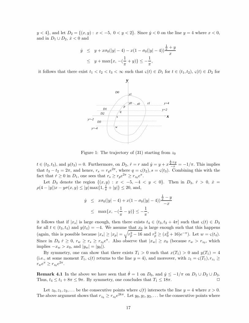
y < 4, and let D2 = (x, y) : x < −5, 0 < y < 2. Since y < 0 on the line y = 4 where x < 0,and in D1 ∪ D2, x < 0 and

y ≤ y + xσ0(|y| − 4) − x(1 − σ0(|y| − 4))1π + y

x

≤ y + maxx, −(1

π+ y) ≤ −

1

π,

it follows that there exist t1 < t2 < t3 < ∞ such that ς(t) ∈ D1 for t ∈ (t1, t2), ς(t) ∈ D2 for

y=-4

y=-2

y=2

y=4z1z0y0

y1

p

q

s

w

D0

D1

D2

D3

x

y

Figure 1: The trajectory of (31) starting from z0

t ∈ (t2, t3), and y(t3) = 0. Furthermore, on D2, r = r and y = y + x1π

+y

−x = −1/π. This implies

that t3 − t2 = 2π, and hence, rs = rqe2π, where q = ς(t2), s = ς(t3). Combining this with the

fact that r ≥ 0 in D1, one sees that rs ≥ rpe2π ≥ rz0e

π.

Let D3 denote the region (x, y) : x < −5, −4 < y < 0. Then in D3, r > 0, x =ρ(4 − |y|)x − yσ(x, y) ≤ |y|max1, 1

π + |y| ≤ 20, and,

y ≤ xσ0(|y| − 4) + x(1 − σ0(|y| − 4))1π − y

−x

≤ maxx, −(1

π− y) ≤ −

1

π,

it follows that if |xs| is large enough, then there exists t4 ∈ (t3, t3 + 4π] such that ς(t) ∈ D3

for all t ∈ (t3, t4) and y(t4) = −4. We assume that x0 is large enough such that this happens

(again, this is possible because |xs| ≥ |xp| =√

r2p − 16 and r2

p ≥ (x20 + 16)e−π). Let w = ς(t4).

Since in D3 r ≥ 0, rw ≥ rs ≥ rz0eπ. Also observe that |xw| ≥ x0 (because rw > rz0 , which

implies −xw > x0, and |yw| = |y0|).

By symmetry, one can show that there exists T1 > 0 such that x(T1) > 0 and y(T1) = 4(i.e., at some moment T1, ς(t) returns to the line y = 4), and moreover, with z1 = ς(T1), rz1 ≥rweπ ≥ rz0e

2π.

Remark 4.1 In the above we have seen that θ = 1 on D0, and y ≤ −1/π on D1 ∪ D2 ∪ D3.Thus, t4 ≤ t1 + 8π ≤ 9π. By symmetry, one concludes that T1 ≤ 18π. 2

Let z0, z1, z2, . . . be the consecutive points where ς(t) intersects the line y = 4 where x > 0.The above argument shows that rzk

≥ rz0e2kπ. Let y0, y1, y2, . . . be the consecutive points where

17

ς(t) intersects the y-axis in the upper half plane. Then (using once more that r ≥ −r and θ = 1on D0) yk ≥ rzk

e−π/2 ≥ rz0e2kπ−π/2 → ∞. This shows that the output y(t) corresponding to

the initial state z0 and the bounded input u ≡ 5 is unbounded, contradicting property (5).

Finally, we modify the above example in the following way to get a ubibs system. Considerthe two-dimensional system:

x = ρ(ϕ(x, y) |u| − 1 − |y|)x − yσ(x, y),y = ρ(ϕ(x, y) |u| − 1 − |y|)y + xσ(x, y),

(32)

where σ, ρ are still defined the same as before, and the function ϕ is a smooth function defined inthe following way. For any point z = (x, y) ∈ C := (x, y) : x > 0, y = 4 with x large enough,let Tz = inft > 0 : ς(t, z) ∈ C, where ς(t, z) denotes the trajectory of (31) with ς(0, z) = z. Itwas shown that |ς(Tz)| ≥ |z| e2π. Now for each k > 0, let Ak be the set z ∈ R

2 : rk ≤ |z| ≤ r′k,where 0 < r1 < r′1 < r2 < r′2 < r3 < r′3 < . . . → ∞ are such that, for any k, there exists somezk ∈ Ak∩C so that for the trajectory ς(t, zk) of (31), it holds that ς(t, zk) ∈ Ak for all t ∈ [0, Tzk

].Then ϕ can be taken as any smooth function such that ϕ(x, y) = 1 on Ak, ϕ(x, y) = 0 for allz = (x, y) such that |z| = (r′k + rk+1)/2 for all k ≥ 1, and 0 ≤ ϕ(x, y) ≤ 1 everywhere else. Inaddition, we assume ϕ(x, y) = 0 on the set A0 := |z| ≤ r1/2.

To show that the system is ubibs, we still let V (x, y) = (x2 + y2)/2. Pick any input u andany initial point z0 = (x0, y0). Let (x(t), y(t)) denote the corresponding trajectory. Let Ak bethe set |z| ≤ r′′k := (r′k +rk+1)/2. Then Ak is forward invariant because on the set |zk| = r′′k,DV (x, y)f(x, y, u) = 2ρ(−1 − |y|)V (x, y) < 0. Hence, if |z0| ≤ r′′k , then |(x(t), y(t))| ≤ r′′k forall t ≥ 0. Observe that A0 is also forward invariant, and if (x(0), y(0)) ∈ A0,

ddtV (x(t), y(t)) ≤

2ρ(−1 − y(t))V (x(t), y(t)) ≤ 0, which implies that V (x(t), y(t)) ≤ V (x(0), y(0)) for all t ≥ 0.Now let σ be any K∞-function such that σ(s) ≥ s for 0 ≤ s ≤ r′′0 , and σ(s) ≥ r′′k+1 forr′′k ≤ s ≤ r′′k+1 for all k ≥ 0. Then V (x(t), y(t)) ≤ σ(|z(0)|) for all t ≥ 0. This shows thatthe system is ubibs. It can also be seen that V still satisfies (30) for system (32), and hence,arguing as before, system (32) is ros.

To show that the system fails to be ios, we again pick the input function u0 ≡ 5. With thisinput, the system satisfies the equations

x = ρ(5ϕ(x, y) − 1 − |y|)x − yσ(x, y),y = ρ(5ϕ(x, y) − 1 − |y|)y + xσ(x, y).

(33)

Observe that, for each k ≥ 1, equations in (33) are the same as in (31) on Ak. For each z ∈ R2,

let ϑ(t, z) denote the trajectory of (33) with the initial state ϑ(0, z) = z. Then, for each k ≥ 1,ϑ(t, zk) = ς(t, zk) for all t ∈ [0, Tzk

]. Let Dk be the complement of the region enclosed by thecurve ϑ(t, zk) : 0 ≤ t ≤ Tzk

and the line segment Lk between zk and ϑ(Tzk) on the line y = 4.

Then Dk is forward invariant by uniqueness and the fact that y > 0 on Lk. This implies thatfor all t > Tzk

, |ϑ(t, zk)| ≥ rk.

For each k ≥ 1, let (xk(t), yk(t)) = ϑ(t, zk). Below we will show that, for each k, thereexists t1 < t2 < t3 < . . . → ∞ such that yk(tl) ≥ rk for all l ≥ 1. It then will follow that

limt→∞

yk(t) ≥ rk. For this purpose, we consider the angular movement θk(t) of ϑ(t, zk). It can beseen that θk(t) satisfies the equation

θ = σ0(|y| − 4) + (1 − σ0(|y| − 4))1π + |y|

max1, |x|.

Since Ak is forward invariant, it holds that |ϑ(t, zk)| ≤ r′′k for all t ≥ 0, and hence,

d

dtθk(t) ≥ min

1,

1π + |yk(t)|

max1, |xk(t)|

≥ min

1,

1π

max1, r′′k

.

18

From this, we know that θk(t) → ∞. This shows that there exist 0 < t1 < t2 < t3 < . . . → ∞such that θk(tl) = 2lπ + π/2. Hence, |yk(tl)| = |ϑ(tl, zk)| ≥ rk for all l ≥ 1. This shows that it

is impossible to have some γ ∈ K such that limt→∞

|yk(t)| ≤ γ(‖u0‖) = γ(5) for all k. We concludethat the system is not ios.

A A Lemma Regarding KL Functions

Lemma A.1 For any KL-function β, there exists a family of mappings Trr≥0 such that

• for each fixed r > 0, Tr : R>0onto−→ R>0 is continuous and strictly decreasing, and T0(s) ≡ 0;

• for each fixed s > 0, Tr(s) is strictly increasing as r increases, and is such that β(r, Tr(s)) <s, and consequently, β(r, t) < s for all t ≥ Tr(s).

Proof. For each r ≥ 0 and each s > 0, let Tr(s) := inft : β(r, t) ≤ s. Then Tr(s) < ∞, forany r, s > 0, β(r, Tr(s)) ≤ s for all r ≥ 0, all s > 0, and it satisfies

Tr(s1) ≥ Tr(s2), if s1 ≤ s2, and Tr1(s) ≤ Tr2(s), if r1 ≤ r2.

Note also that T0(s) = 0 for all s > 0. Following exactly the same steps as in the proof of [11,Lemma 3.1], one can modify Tr(s) to obtain Tr(s) so that for each fixed r ≥ 0, Tr(·) is decreasingand continuous; and for each fixed s, T(·)(s) is increasing. Finally, one lets Tr(s) = Tr(s)+ r

1+s .Then Tr(s) satisfies all conditions required in Lemma A.1.

References

[1] D. Angeli and E. D. Sontag, Forward completeness, unboundedness observability, and theirLyapunov characterizations, Systems & Control Letters, to appear.

[2] B.A. Francis, The linear multivariable regulator problem, SIAM J. Control & Opt. 15

(1977), pp. 486–505.

[3] A. Isidori, Nonlinear Control Systems, Third Edition, Springer-Verlag, London, 1995.

[4] , Global almost disturbance decoupling with stability for non minimum-phase single-input single-output nonlinear systems, Systems & Control Letters, 28 (1996), pp. 115–122.

[5] Z.-P. Jiang, A. Teel, and L. Praly, Small-gain theorem for ISS systems and applications,Mathematics of Control, Signals, and Systems, 7 (1994), pp. 95–120.

[6] H.K. Khalil, Nonlinear Systems (Second Edition), Macmillan, New York, 1996.

[7] M. Krstic and H. Deng, Stabilization of Uncertain Nonlinear Systems, Springer-Verlag,London, 1998.

[8] M. Krstic, I. Kanellakopoulos, and P. V. Kokotovic, Nonlinear and Adaptive ControlDesign, John Wiley & Sons, New York, 1995.

[9] V. Lakshmikantham, S. Leela, and A. A. Martyuk, Practical Stability of Nonlinear Sys-tems, World Scientific, New Jersey, 1990.

19

[10] Y. Lin, Lyapunov Function Techniques for Stabilization, PhD thesis, Rutgers, The StateUniversity of New Jersey, New Brunswick, New Jersey, 1992.

[11] Y. Lin, E. D. Sontag, and Y. Wang, A smooth converse Lyapunov theorem for robuststability, SIAM Journal on Control and Optimization, 34 (1996), pp. 124–160.

[12] W. M. Lu, A class of globally stabilizing controllers for nonlinear systems, Systems &Control Letters, 25 (1995), pp. 13–19.

[13] Marino, R., and P. Tomei, Nonlinear output feedback tracking with almost disturbancedecoupling. IEEE Trans. Automat. Control 44(1999). pp. 18–28.

[14] W.J. Rugh, Linear System Theory, Prentice-Hall, Englewood Cliffs, 1993.

[15] R. Sepulchre, M. Jankovic, and P.V. Kokotovic, Integrator forwarding: a new recursivenonlinear robust design, Automatica 33(1997): 979-984.

[16] E. D. Sontag, Smooth stabilization implies coprime factorization, IEEE Transactions onAutomatic Control, AC-34 (1989), pp. 435–443.

[17] , Some connections between stabilization and factorization, in Proc. IEEE Conf.Decision and Control, Tampa, Dec. 1989, IEEE Publications, 1989, pp. 990–995.

[18] , Mathematical Control Theory, Deterministic Finite Dimensional Systems, SecondEdition, Springer-Verlag, New York, 1998.

[19] E. D. Sontag and Y. Wang, On characterizations of the input-to-state stability property,Systems & Control Letters, 24 (1995), pp. 351–359.

[20] , Detectability of nonlinear systems, in Proc. Conf. on Information Science and Sys-tems (CISS 96), Princeton, NJ, 1996, pp. 1031–1036.

[21] , Output-to-state stability and detectability of nonlinear systems. Systems & ControlLetters, 29 (1997), pp. 279–290.

[22] , New characterizations of the input to state stability property, IEEE Transactionson Automatic Control, 41 (1996), pp. 1283–1294.

[23] , A notion of input to output stability, Proc. European Control Conf., Brussels, July1997, Paper WE-E A2, CD-ROM file ECC958.pdf, 6 pages.

[24] , Lyapunov characterizations of input to output stability, submitted.

[25] Tsinias, J., Input to state stability properties of nonlinear systems and applications tobounded feedback stabilization using saturation, ESAIM Control Optim. Calc. Var.2(1997): 57-85.

[26] V. I. Vorotnikov, Stability and stabilization of motion: Research approaches, results, dis-tinctive characteristics, Automation and Remote Control, 54 (1993).

[27] F.W. Wilson, Jr., Smoothing derivatives of functions and applications, Transactions of theAmerican Mathematical Society, 139 (1969), pp. 413–428.

[28] T. Yoshizawa, Stability Theory and the Existence of Periodic Solutions and Almost Peri-odic Solutions, Springer-Verlag, New York, 1975.

20