Electronic copy available at: http://ssrn.com/abstract=1874668

On the High-Frequency Dynamics of

Hedge Fund Risk Exposures�

Andrew J. Pattony

Duke University

Tarun Ramadoraiz

University of Oxford

14 December 2011

Abstract

We propose a new method to model hedge fund risk exposures using relatively high frequency

conditioning variables. In a large sample of funds, we �nd substantial evidence that hedge fund

risk exposures vary across and within months, and that capturing within-month variation is

more important for hedge funds than for mutual funds. We consider di¤erent within-month

functional forms, and uncover patterns such as day-of-the-month variation in risk exposures.

We also �nd that changes in portfolio allocations, rather than changes in the risk exposures of

the underlying assets, are the main drivers of hedge funds�risk exposure variation.

Keywords: beta, time-varying risk, performance evaluation, window-dressing, hedge funds,

mutual funds.

JEL Codes: G23, G11, C22.

�We thank the Oxford-Man Institute of Quantitative Finance for �nancial support, Alexander Taylor and Sushant

Vale for dedicated research assistance, and Nick Bollen, Michael Brandt, Mardi Dungey, Jean-David Fermanian,

Robert Kosowski, Olivier Scaillet, Kevin Sheppard, Melvyn Teo, and seminar participants at the Fuqua School

of Business, the Oxford-Man Institute Hedge Fund Conference, the CREST-HEC Hedge Fund Conference, the 2010

SoFiE annual conference, Lancaster University, the University of Tasmania, and the 2011 Western Finance Association

conference for useful comments.yDepartment of Economics, Duke University, and Oxford-Man Institute of Quantitative Finance. 213 Social

Sciences Building, Durham NC 27708-0097, USA. Email: andrew.patton@duke.edu.zSaïd Business School, Oxford-Man Institute of Quantitative Finance, and CEPR. Park End Street, Oxford OX1

1HP, UK. Email: tarun.ramadorai@sbs.ox.ac.uk.

Electronic copy available at: http://ssrn.com/abstract=1874668

On the High-Frequency Dynamics ofHedge Fund Risk Exposures

Abstract

We propose a new method to model hedge fund risk exposures using relatively high frequency

conditioning variables. In a large sample of funds, we �nd substantial evidence that hedge fund

risk exposures vary across and within months, and that capturing within-month variation is more

important for hedge funds than for mutual funds. We consider di¤erent within-month functional

forms, and uncover patterns such as day-of-the-month variation in risk exposures. We also �nd

that changes in portfolio allocations, rather than changes in the risk exposures of the underlying

assets, are the main drivers of hedge funds�risk exposure variation.

1 Introduction

An important feature of hedge funds is the speed at which they alter their investments in response

to changing market conditions. Static analyses of hedge funds�risk exposures are likely to miss

these rapid changes in their strategies or leverage ratios, and several new approaches have been

proposed to model the dynamics of these risk exposures.1 One factor that must be taken into

consideration is the high frequency (often daily or even higher) at which hedge fund risk exposures

change.2 However, the new approaches thus far proposed to model dynamic risk exposures are

limited to tracking such changes only at the monthly frequency, as this is the reporting frequency

for performance data in all of the main hedge fund databases.

We propose a new method to surmount this obstacle, and to better understand the high-

frequency dynamics of hedge fund risk exposures. The starting point for our approach is the widely-

used Ferson and Schadt (1996) model, which we extend to employ higher frequency conditioning

information. To circumvent the lack of high frequency data on hedge fund performance, we posit

a daily factor model for hedge fund returns and then aggregate this up to the monthly frequency

for estimation. We demonstrate that the method is able to accurately track the dynamics of daily

variation in hedge fund risk exposures, by testing it on daily indexes of hedge fund returns, in

addition to simulations.

The higher-frequency version of Ferson and Schadt (1996) in which daily risk-exposures evolve

as a linear function of observable instruments, (which we dub the �linear model�), is the �rst of

three economically-motivated functional forms for high-frequency risk exposures that we consider.

The second model that we consider allows for intra-month seasonalities in risk exposures (the �day-

of-the-month model�), and the third model allows risk exposures to vary abruptly when observable

instruments hit pre-speci�ed threshold values (we term this the �threshold model�). By allowing

for a variety of economically plausible ways in which risk exposures may evolve, we attempt to

mitigate the inevitable loss of information that arises when using monthly returns to infer intra-

1The literature on modeling hedge fund returns using static models is extensive. A partial list includes Fung

and Hsieh (1997, 2004a,b), Ackermann, McEnally and Ravenscraft (1999), Liang (1999), Agarwal and Naik (2004),

Kosowski, Naik and Teo (2006), Agarwal, Fung, Loon, and Naik (2009), Chen and Liang (2007), Fung, Hsieh, Naik

and Ramadorai (2008), Patton (2009) and Jagannathan, Malakhov and Novikov (2010).2See �Wall Street�s New Race Toward Danger�, Barron�s, March 8, 2010 and �Traders Piqued By the Picosecond,

But Physics Intervenes,�Wall Street Journal, March 10, 2010.

1

monthly dynamics. More importantly perhaps, the results from these di¤erent speci�cations allow

us to better understand hedge fund behavior during non-reporting intervals that have thus far been

impervious to scrutiny.

We implement these dynamic risk exposure models on a cross-section of 14,194 individual hedge

funds and funds-of-funds over the period 1994 to 2009, and �nd that they perform very well at

explaining hedge fund returns. In particular, the models generate adjusted R2 statistics that are

a substantial improvement over a static-parameter benchmark model: the average adjusted R2 for

our linear speci�cation, is 49% higher than the corresponding average for the Fung-Hsieh bench-

mark model. We also �nd that including higher frequency conditioning information substantially

improves the performance of our model: the percentage of hedge funds for which we �nd statisti-

cally signi�cant factor exposure variation nearly doubles, from 12% to 22%, when we include daily

information as well as monthly information in our estimated speci�cations. In contrast, when we

estimate our model on a set of 32,913 equity and bond mutual funds, adding daily information to

the monthly information set leaves the percentage of funds for which we �nd statistically signi�-

cant factor exposure variation virtually unchanged. In short, there is signi�cant daily variation in

hedge fund risk exposures, and accounting for this daily variation is necessary to characterize hedge

fund behavior accurately. However, daily risk-exposure variation does not seem to be as important

for mutual funds � a fact which is perhaps unsurprising given short-sales restrictions and other

constraints on mutual fund portfolio alterations.

The models that we propose provide new and valuable insights into hedge fund behavior at high

frequencies. One particularly interesting �nding from the day-of-the-month model is that there are

signi�cant intra-month seasonalities in hedge fund risk-exposures. In particular, we �nd that hedge

fund risk exposures are relatively high at the beginning of the month and decline steadily as the

month progresses, reaching their lowest point at the end of the month just prior to the date at

which hedge funds report returns to databases. There are several possible explanations for this

phenomenon. One innocuous explanation is that this pattern re�ects regular expirations of short-

lived derivative positions held by funds. Another less innocuous explanation is that this pattern

constitutes evidence of intra-month window-dressing by hedge funds. This explanation links our

result to the extensive literature on mutual-fund and pension-fund window-dressing pioneered by

Lakonishok et al. (1991), as well as the growing body of literature by authors such as Bollen and

Krepely-Pool (2009) and Agarwal et al. (2011) on unusual monthly patterns in hedge fund returns.

2

The threshold model also yields useful insights, one of which is that hedge funds have a ten-

dency to abruptly cut positions in response to signi�cant market events. For example, when market

returns fall or when illiquidity rises signi�cantly within the month, hedge funds signi�cantly cut

exposures to small stocks. This evidence is akin to that provided at lower frequencies by Brun-

nermeier and Pedersen (2005), who document that hedge funds �rode�the technology bubble, and

�ts the description of destabilizing rational speculation provided in DeLong et al. (1990). Further-

more, when S&P500 volatility rises signi�cantly within the month, we �nd evidence that hedge

funds cut back their positions across all risky assets, appearing to retreat towards cash at such

times. This provides useful evidence in favour of Ferson and Schadt�s (1996) conjecture that the

enhanced mutual fund alpha that they detect using a time-varying beta model is on account of

managers adjusting risk exposures in line with movements in aggregate volatility, and the more

recent extension by Lo (2008), who decomposes fund manager performance into a �passive�com-

ponent, and an �active�component which arises from the correlation between changing portfolio

weights and returns. Indeed, as we describe below, we also �nd improved performance from our

time-varying beta model relative to the alpha obtained from a static factor model.

In the discussion thus far, we have tended to interpret evidence of time-varying risk exposures

in terms of fund managers actively shifting portfolio allocations. Of course, it is possible that

time-variation in underlying asset betas could result in changes in fund risk exposures even when

fund managers pursue passive buy-and-hold strategies. To evaluate their relative magnitudes, we

posit a simple decomposition of fund beta variation into weight variation, asset beta variation,

and weight-beta covariation. We then estimate this decomposition using matched 13-F data on all

long-short equity hedge funds in our sample.3 Using these data, we �nd that on average from 1989

to 2010, weight variation accounts for 73% of total fund beta variation and asset beta variation

constitutes 17%, with covariances accounting for the remainder. During the recent �nancial crisis

(2007 to 2010), weight variation accounts for an increased share, 84% of the total, with the share of

pure asset beta variation practically unchanged. In sum, the evidence indicates that the primary

source of hedge funds�dynamic risk exposures is their changing portfolio weights.

3The quarterly 13-F �lings data track long equity positions of institutional investment managers, hence this analysis

is naturally restricted to the subset of long-short equity fund managers in our data. This analysis complements our

high-frequency analysis, providing us with additional information on the underlying causes for movements in hedge

fund risk exposures. We thank an anonymous referee for suggesting that we pursue this.

3

Finally, we analyze the implications of our method for performance measurement. We �nd,

similar to Ferson and Schadt (1996), that annualized alpha for funds with signi�cantly time-varying

factor exposures rises on average by a percentage point when estimated using our model rather than

the constant model. However this �nding masks much bigger changes at the individual fund level

�we �nd a mean absolute di¤erence of 2.7% to 4.6% between annualized alphas estimated using

the constant model and our three time-varying exposure models.

The outline of the paper is as follows. The remainder of this section situates our paper in the

literature on the dynamic performance evaluation of managed investments. Section 2 describes

our modelling approach and Section 3 describes the data used in our analysis. Section 4 presents

analyses which verify that our proposed method works well in practice, and Section 5 presents our

main empirical results. Section 6 looks at the sources of variation in hedge fund risk exposures and

Section 7 concludes.

1.1 Related literature

Our paper contributes to the literature on dynamic performance measurement for actively managed

investment vehicles, a topic that has recently experienced a resurgence of interest. For example,

Mamaysky, Spiegel and Zhang (2008) use a Kalman �lter-based model to track mutual fund risk

exposures as latent random variables. Bollen and Whaley (2009) consider this approach for hedge

funds, but recommend instead the use of optimal change-point regressions (a la Andrews et al.

(1996)), to estimate structural breaks in hedge fund factor loadings. The change-point approach

models risk exposures as constant between change-points, with abrupt changes to a new value at the

change-points. The model pinpoints the time at which risk exposures change, although it is unable

to provide insights into the underlying economic drivers of these changes. Our model provides a

simple but economically interpretable alternative to this change-point approach, in which time-

varying betas are functions of observable conditioning variables.4 The intellectual predecessor of

our approach is Ferson and Schadt (1996), who use well-known predictors of returns as proxies for

publicly available information, and employ these instruments to estimate an unconditional version

4Patton and Ramadorai (2010) test the statistical performance of the approach in this paper as well as that of the

change-point model on a large cross-section of hedge funds and funds-of-funds. They �nd that the �linear�model

described in 2.2.1 below yields better statistical performance than the change-point model, but that there are gains

to combining the two approaches.

4

of their conditional model for the performance evaluation of mutual funds.5

Our main contribution lies in the use of daily conditioning information to evaluate monthly

reported performance. There have been other attempts to combine monthly returns and intra-

monthly information to ascertain the higher-frequency variation in risk factor loadings, following

an in�uential paper by Goetzmann, Ingersoll, and Ivkovic (2000), which shows that Henriksson-

Merton timing measures (discussed below) estimated from monthly data are biased in the presence

of daily timing ability. Goetzmann et al. attempt to correct for this bias by cumulating daily put

values on the S&P 500 for each month in their sample, which they incorporate as an additional

regressor in their market-timing speci�cations (Ferson and Khang (2002) also present a conditional

version of the holdings-based performance evaluation method that avoids the Goetzmann et al.

bias). Ferson, Henry, and Kisgen (2006) consider an underlying continuous-time process for the

term structure of interest rates to study monthly government bond fund performance, and uncover

that time-averages of daily interest rate movements are pivotal in explaining bond mutual fund

performance. While similar in spirit, our approach di¤ers in a number of ways from the methods

followed in these papers. First, our approach relies on the use of intra-monthly products of factors

and interaction variables, rather than on time-aggregated higher frequency factors alone (which

we additionally consider in the day-of-the-month model). Second, we posit several di¤erent daily

models for hedge fund returns, which we use to uncover the actual intra-monthly patterns in hedge

fund risk exposures. This allows us to economically interpret hedge funds� high-frequency risk

exposure dynamics in addition to mitigating the inevitable loss of information that arises when

attempting to infer intra-monthly dynamics using only monthly returns.

It is worth brie�y mentioning a set of models which use conditioning information to detect

time-variation in managerial risk exposures in an attempt to �nd evidence of market-timing ability.

One approach that is often employed (for example, by Treynor and Mazuy (1966), Lehmann and

Modest (1987) for mutual funds, and Chen and Liang (2007) for hedge funds) is to extend the

standard single factor market model by including quadratic terms, or, as in Henriksson and Merton

5Chen and Knez (1996) derive contemporaneous insights into conditional performance evaluation. These models

are also related to Jagannathan and Wang (1996), who focus on risk adjustment for equities rather than performance

evaluation. See also Ferson and Harvey (1991), Evans (1994) and others. Mamaysky, et al. (2008) also �nd that

adding observable variables to their model for mutual fund returns improves its performance, relative to a model

solely with a latent factor driving variation in risk exposures.

5

(1981), by interacting the market return with an indicator variable for the sign of the market

return. Such regressions can be motivated using the model of Admati, Bhattacharya, P�eiderer

and Ross (1986), in which a successful market-timing fund manager receives a noisy signal about

the one period ahead market return �an idea that can be generalized to consider private signals

about market attributes such as future market liquidity, as in Cao, Chen and Liang (2009). As

a consequence of the use of contemporaneous conditioning information, these models have two

measures of managerial ability, namely, the �timing� coe¢ cient on the interaction term between

the factor and the contemporaneous variable representing the signal, and the �selectivity,�i.e., the

intercept from the unconditional estimation of the conditional model.6 In contrast, in conditional

performance evaluation models such as the one in this paper, the conditioning information is lagged,

meaning that estimated alphas are measures of fund performance over and above that which can

be garnered using public information signals, and can be interpreted as measures of managerial

ability in the usual manner.7

Finally, our use of daily returns on hedge fund indexes to validate our proposed method (see

Section 4) adds to the sparse literature which uses daily data on investment managers�returns to

measure their performance. Busse (1999) �nds that mutual funds have signi�cant volatility timing

ability using daily returns data. Bollen and Busse (2001), also using daily data, con�rm that

mutual funds have signi�cant market timing ability. Chance and Hemler (2001) use daily executed

recommendations of market-timers, and �nd that they have signi�cant daily timing ability which

vanishes when their performance is evaluated at the monthly frequency.

2 Modelling time-varying hedge fund risk exposures

In this section we �rst describe the conditional performance evaluation approach of Ferson and

Schadt (1996), which is the initial point of departure for our model. We then present the three

variants of our model which are estimated in Section 5. To simplify the description of the various

6Holdings-based performance evaluation approaches have also been used to separate timing ability from selectivity

(See Daniel, Grinblatt, Titman and Wermers (1997), Chen, Jegadeesh and Wermers (2000), and Da, Gao and

Jagannathan (2009)). Graham and Harvey (1996) use asset allocation recommendations in investment newsletters

to evaluate whether they help investors to time the market.7Note that the approach in Ferson and Schadt (1996) is extended by Christophersen, Ferson, and Glassman (1998)

to include the possibility of time-variation in alpha, this is also a possible extension to our approach.

6

models we consider a simple one-factor model for capturing risk exposures, although in our empirical

analysis in Section 5 we allow for multiple factors.

2.1 Models with monthly variation in risk exposures

Ferson and Schadt (1996) present a model in which betas evolve as a linear function of observable

variables measured monthly:

rit = �i + �itft + "it (1)

where �it = �i + iZt�1 (2)

That is, the return on fund i is driven by a factor, ft, with the factor loading varying according to

some zero-mean variable Zt�1.8 Substituting in the equation for �it we obtain:

rit = �i + �ift + iftZt�1 + "it (3)

which is easily estimated using OLS regression. Note that the constant-beta model is nested in the

above speci�cation, and the signi�cance of time variation in beta for the ith fund can be tested via

a standard Wald test of the following hypothesis:

H(i)0 : i = 0 vs. H(i)

a : i 6= 0 (4)

2.2 Models with daily variation in risk exposures

Many hedge funds alter or turn over positions very frequently, thus it is possible that a hedge fund�s

risk exposure changes substantially within a month. This observation necessitates an extension of

the above approach for modelling time-varying risk exposures. Consider the daily returns on hedge

fund i; denoted r�id; and a corresponding daily factor model for these returns:

r�id = �i + �idf�d + "

�id (5)

Let us assume that the factor loadings for this fund vary as a function of some conditioning variable,

Z which is observable at a daily frequency:

�id = gi(Z):

8De-meaning Zt�1 ensures that we can interpret �i as the average level of risk exposure. Using Zt�1 rather than

Zt means that we can interpret �i as a measure of the fund�s risk-adjusted performance, as per the discussion in

Section 1.1.

7

We can consider various functional forms for gi(Z). The simplest is the direct analogue to the

Ferson and Schadt approach, namely, where gi(Z) is linear in Z.

2.2.1 A linear model for factor exposures

To better understand how the linear model relates to Ferson and Schadt, let Z�d denote the con-

ditioning variable measured at the daily frequency and Zd denote this variable measured at the

monthly frequency (that is, Zd will be constant within each month and jump to a new level at the

start of each month). Then the linear model for gi(Z) can be written as:

�id = gi(Z) = �i + iZd�1 + �iZ�d�1 (6)

Substituting into (5) we obtain a simple interaction model for daily hedge fund returns:

r�id = �i + �if�d + if

�dZd�1 + �if

�dZ

�d�1 + "

�id (7)

Returns on individual hedge funds are currently only available monthly, and so to estimate this

model we need to aggregate returns from the daily frequency up to the monthly frequency.9 De�ne

the monthly return on fund i as:

rit �X

d2M(t)

r�id (8)

whereM (t) is the set of days in month t. De�ne ft and Zt similarly, and let nt denote the number

of days in month t. Then the speci�cation for monthly hedge fund returns becomes:

rit = �int + �ift + iftZt�1 + �iX

d2M(t)

f�dZ�d�1 + "it (9)

Note that the dependent variable above is now the monthly return on hedge fund i; and all variables

on the right-hand side are also measured monthly. The new variable that appears in this speci�ca-

tion relative to the Ferson-Schadt style speci�cation in equation (3) is of the formX

f�dZ�d�1. This

is a monthly aggregate of a daily interaction term, and it captures variations in hedge fund risk

9We use log returns, and so the monthly return is simply the sum of the daily returns. In this case, however, the

linear factor model is only approximate. An alternative is to use simple returns, making the factor model exact, but

introducing an approximation error when aggregating to monthly returns. In the Internet Appendix we show that

the approximation error introduced by both of these approaches is negligible for our data.

8

exposures at the daily frequency.10 If the factor, f�d ; and the conditioning variable, Z�d�1; are both

available at the daily frequency, then under the assumption that "�id is serially uncorrelated and un-

correlated with f�s for all (d; s) we are able to estimate the coe¢ cients of this model using standard

OLS. As above, for valid statistical inference we need to account for potential heteroskedasticity

and non-normality in the residuals. In Section 4 we present analyses based on real daily hedge fund

index returns and simulated returns, both of which con�rm that this modeling approach works well

in realistic applications.

The constant-beta model is nested in the above speci�cation, and the signi�cance of time

variation in beta can be tested via a standard Wald test of the following hypothesis:

H(i)0 : i = �i = 0 vs. H(i)

a : i 6= 0 [ �i 6= 0 (10)

Furthermore, we can test whether we �nd signi�cant evidence of daily variation in hedge fund risk

exposures, controlling for monthly variation, by testing that the coe¢ cient on the daily interaction

term is zero:

H(i)0 : �i = 0 vs. H(i)

a : �i 6= 0 (11)

While it is anticipated that hedge funds do adjust their risk exposures within the month, our ability

to detect those changes depends on whether we can �nd observable daily interaction variables, Z�d ,

that are correlated with those changes. We pick four economically-motivated Z variables in this

paper, described in Section 3.3 below.

2.3 Day-of-the-month e¤ects in factor exposures

Lakonishok et al. (1991) �nd that pension fund managers tend to increasingly sell losing stocks in

the fourth quarter of the year, when funds�portfolios are closely examined by the sponsors. They

suggest that this constitutes evidence of window-dressing, where managers alter their portfolios to

impress sponsors.

Most hedge funds claim to generate �absolute returns,� that are uncorrelated (i.e., zero-beta)

with widely-used benchmarks. Akin to pension funds and mutual funds, hedge funds also have

10We also considered a MIDAS weighting function, in the spirit of Ghysels, Santa-Clara, and Valkanov (2006), for

intra-monthly risk-exposure variation as a function of more lags of the daily conditioning variables (Z�d ). This more

general speci�cation was found to be statistically indistinguishable from the simpler model that we present here.

9

periodic (monthly) reporting intervals to publicly available databases.11 Within these reporting

intervals, hedge funds are at liberty to pursue strategies that might not necessarily be zero-, or

even low-beta. Indeed, managers could pursue strategies which have low monthly-average betas on

benchmarks despite having quite high betas at periods within these months. One such strategy is for

managers to have high exposures just following monthly reporting dates, and lower exposures just

preceding the subsequent reporting date. Another possibility is that managers attempt absolute-

return strategies at the beginning of the month, and put on leveraged positions on benchmarks at

the end of the month so as to garner higher returns.

To detect such intra-month seasonalities, we consider the following speci�cation:

�id = gi (Z) =��i� (d; ��;i) + iZd�1 + �iZ

�d�1; (12)

where the second and third terms in the expression are the same as in the linear model. For

the leading term, �i (d; ��) ; we follow Ghysels, Santa-Clara, and Valkanov (2006), and Andreou,

Ghysels, and Kourtellos (2010) and use an �exponential Almon�function, which provides a �exible

parametric function of the day of the month. We model this as a fraction of the month, d=nt; to

accommodate months with di¤ering numbers of days.

� (d; ��;i) =!idX

d2M(t)!id; (13)

!id � exp

(�i1

d

nt+ �i2

�d

nt

�2):

Relative to the linear model, the gi(Z) function now includes an �intercept�that detects the variation

of betas on speci�c days of the month. The Internet Appendix plots a range of possible shapes

that can be taken by � (d; �i;�), which encompasses a number of economically-interesting patterns

including the possibility of window-dressing described above. Importantly, this speci�cation also

includes the case that � (d; ��;i) is �at throughout the month, which indicates the absence of a

day-of-the-month e¤ect, and thus allows us to formally test for the presence of these e¤ects. In our

empirical analysis we also consider the simple case of a pure day-of-the-month speci�cation:

�id = gi (Z) =��i� (d; ��;i) ; (14)

11One di¤erence, of course, is that hedge funds report only returns, not actual holdings. Another is that reporting

for pension funds is mandatory, whereas it is discretionary for hedge funds. One potentially important implication

of this discretionary reporting for our tests, highlighted by Getmansky et al. (2004), is excessive hedge fund return

smoothness. We control for this possibility using their suggested approach in our robustness checks.

10

and examine whether evidence exists for purely deterministic variation in risk exposures.

2.4 A threshold model for factor exposures

Both models presented above assume that beta variation is linear in the conditioning variable. We

next consider a nonlinear description for these dynamics based on a threshold model, where beta

is assumed to switch from one value to another once a threshold for the conditioning variable is

reached:

�id =

8<: �i;lo; Z�d�1 � �Z

�i;hi; Z�d�1 >�Z

(15)

For this model we use conditioning variables that cumulate gains, losses, or volatility through each

month, and we choose the threshold, �Z; as a function of the month-end values of the conditioning

variable. For example, one conditioning variable that we consider here is the cumulated return

on a market index, and so this speci�cation posits that beta remains at one level so long as the

cumulated market return remains above some threshold, but if the market return falls too far

(relative to the average movement in market returns in a month) then the beta switches to a new

level.12 We also consider variables that cumulate volatility, or changes in liquidity, as described

below.

3 Data

3.1 Hedge fund and fund of funds data

We use a large cross-section of hedge funds and funds-of-funds over the period from January 1994 to

June 2009, which is consolidated from data in the HFR, CISDM, TASS, Morningstar and Barclay-

Hedge databases. The Internet Appendix contains details of the process followed to consolidate

these data. The funds in the combined database come from a broad range of vendor-classi�ed

strategies, which are consolidated into ten main strategy groups: Security Selection, Global Macro,

12We thank an anonymous referee for suggesting that we consider a threshold model. This speci�cation is motivated

by the idea that when a hedge fund manager breaches a threshold for monthly pro�ts/losses, the beta is set to a

new level. As hedge fund returns are not available at the daily frequency, we cannot use them as daily conditioning

variables. However by using variables that correlate with hedge fund daily returns we hope to capture this e¤ect if

it is present in the data.

11

Relative Value, Directional Traders, Funds of Funds, Multi-Process, Emerging Markets, Fixed In-

come, CTAs, and Other (which contains funds with missing vendor strategy classi�cations).13

Table I reports summary statistics on the hedge fund data. To overcome the well-known problem

of return smoothing in monthly reported hedge fund returns, we use �unsmoothed�returns in our

analysis, which are estimated from raw returns fund-by-fund using the Getmansky, Lo, and Makarov

(2004) moving average model, with two lags (in the Internet Appendix, we verify our results using

four lags, as well as raw returns). The means of the reported returns and unsmoothed returns are

similar, but as expected the distribution of the �unsmoothed�returns is slightly more disperse. The

median fund has assets under management of USD 32MM, while the mean is much larger, at USD

167MM, re�ecting the signi�cantly skewed size distribution that several other studies (Getmansky

(2004), Teo (2010)) have highlighted. The median management fee and incentive fees are 1:5%

and 20% respectively, consistent with earlier literature (Agarwal, Daniel and Naik (2009)), and the

withdrawal restrictions are also comparable to earlier literature (Aragon (2005)). Panel B of the

table shows that the lengths of the return histories for the funds in the sample correspond closely

to that reported by Bollen and Whaley (2009), with around half of our funds having 5 or more

years of data available, and around 17% of our funds having less than 3 years of data. Finally,

Panel C reports the distribution of funds across strategies: the two largest strategies are Security

Selection (20.8%) and Funds of Funds (23.3%), while the two smallest strategies (not including

�Other,� which captures those funds with unreported strategies) are Relative Value (1.0%) and

Emerging Markets (3.4%). Given that our complete sample contains 14,194 individual funds, even

the smallest strategy group has 146 distinct hedge funds, which enables us to undertake relatively

precise strategy-level analyses.

3.2 Hedge fund factors

Throughout our analysis, the underlying factor model that we use is the seven-factor model of

Fung and Hsieh (2004a,b). This model has been used in numerous previous studies, see Bollen and

Whaley (2009), Teo (2009), and Ramadorai (2011). The set of factors comprises the excess return on

the S&P 500 index (SP500); a small minus big factor (SMB) constructed as the di¤erence between

13The set contains both live and dead funds. The distribution of live versus defunct funds is roughly similar across

the databases, and the total percentage of defunct funds is 46%, which is comparable to the ratio reported in Agarwal,

Daniel and Naik (2009) of 48%, although their sample period ends in 2002.

12

the Wilshire small and large capitalization stock indexes; the excess returns on portfolios of lookback

straddle options on currencies (PTFSFX), commodities (PTFSCOM), and bonds (PTFSBD), which

are constructed to replicate the maximum possible return to trend-following strategies on their

respective underlying assets;14 the yield spread of the U.S. 10-year Treasury bond over the 3-

month T-bill, adjusted for the duration of the 10-year bond (TCM10Y); and the change in the

credit spread of Moody�s BAA bond over the 10-year Treasury bond, also appropriately adjusted

for duration (BAAMTSY).

3.3 Variables associated with changes in risk exposures

We consider a small set of economically motivated variables to identify increases or decreases

in hedge funds�exposure to systematic risks. These four variables correspond to four underlying

drivers of managerial decisions to alter portfolio allocations, namely, liquidity, funding and leverage,

volatility, and performance.15

There is a growing recognition of the impact of liquidity on hedge fund and mutual fund per-

formance. Pollet and Wilson (2008) document that mutual funds rarely diversify in response to

increases in their asset base, and associate their result with limits to the scalability of fund port-

folios, such as price impact or liquidity constraints. Aragon (2005) and Sadka (2009) both �nd

that liquidity risk is an important determinant of hedge fund returns, and one that is not cap-

tured by the Fung-Hsieh (2004a) seven factors. Following Cao, et al. (2009), we consider the case

that managers may attempt to vary their exposure to risk factors in such a manner as to mitigate

the in�uence of price impact �as liquidity rises (falls), we expect that the absolute magnitude of

risk exposures will rise (fall) as funds more (less) frequently enter or exit positions. To capture

systematic time-series variation in liquidity at both monthly and daily frequencies we employ the

funding liquidity measure proposed by Garleanu and Pedersen (2009), namely the TED spread (the

3-month LIBOR rate minus the 3-month T-bill rate).

Turning to the second possible driver, hedge fund managers�exposures to systematic risk factors

will vary with the level of leverage that they employ if their long and short positions do not exactly

14See Fung and Hsieh (2001) for a detailed description of the construction of these primitive trend-following (PTF)

factors.15 In an earlier version of this paper, Patton and Ramadorai (2010), we considered a set of 19 conditioning variables

spanning the same four groups of variables, and the signi�cance of the best-�tting conditioning variable for each fund

was tested using the �reality check�of White (2000).

13

o¤set one another along the dimension of factor exposure (see Rubin, Greenspan, Levitt, and Born

(1999) who document that hedge funds take on signi�cant leverage). The leverage available to

hedge funds will vary with the costs of borrowing, which we capture using the �rst di¤erence of

the level factor (the constant maturity three month U.S. T-bill rate).

The third variable that we consider is market volatility. As �nancial market volatility rises,

hedge fund managers wishing to maintain fund return volatility constant may trim risk exposures,

a la Ferson and Schadt (1996). We therefore include the VIX index (see Whaley (2000)), which is

a measure of volatility extracted from the prices of options on the S&P 500 index. We also employ

a measure of �realized volatility�(RV) based on intra-daily data on the S&P 500 index, when we

estimate the threshold model.16

Finally, hedge fund managers are often implicitly or explicitly benchmarked to commonly avail-

able indexes. When the returns on these benchmarks are high, managers may be tempted to

increase their risk-factor loadings to avoid the perception that they are underperforming, and vice

versa. With this in mind, we also include returns on the S&P 500 as a conditioning variable.

All told, we have a set of 4 possible conditioning variables in our set: dLevel, the TED spread,

the S&P 500 return, and VIX. As the three variables other than the S&P 500 returns are highly

serially correlated, we use a simple exponentially weighted moving average (EWMA) model (with

the optimal EWMA smoothing coe¢ cient estimated for each series using non-linear least squares)

to obtain their �surprise�component, and use this in place of the levels of these variables17.

4 The accuracy of estimates of daily betas using monthly returns

In this section we study the accuracy of our proposed method for estimating daily variations in

the factor exposures of hedge funds using only monthly returns on these funds. We analyze this

problem in two ways, and �nd support for our method in both cases. While data on individual

hedge fund returns is almost invariably available only at the monthly frequency, daily data on

16These realized volatilities are based on 5-minute prices and were obtained from the Oxford-Man Institute�s

�Realized Library� data, available at http://realized.oxford-man.ox.ac.uk/. See Heber, et al. (2009) for details on

how these measures are computed. The S&P 500 RV series is available from January 1996 until February 2009.

Outside of this period, we use the simple squared returns as the volatility measure.17The �rst-order autocorrelations of the resulting �surprise� components of these variables are 0.21, 0.20, -0.08,

0.09 (monthly) and 0.12, -0.06, 0.02, 0.10 (daily).

14

a collection of hedge fund style index returns has recently become available. These daily index

returns are an ideal, real-world dataset on which to check the accuracy of our method. Our �rst

approach is to employ this daily data on hedge fund index returns, and to compare the results that

are obtained when estimating the model on daily data with those that are obtained when using our

method on the monthly returns on these indexes. Our second approach, described in the Internet

Appendix, is to conduct a simulation study that is calibrated to match the key features of hedge

fund returns, and study the performance of the proposed method under di¤erent features of the

return-generating process.

4.1 Results using daily hedge fund index returns

Daily returns on hedge fund style indexes have recently become available from Hedge Fund Research

(HFR), see Distaso et al. (2009) for an analysis of these indexes. We use these data to check whether

the estimates of hedge fund factor exposures that we obtain based only on monthly returns are

similar to those that would be obtained if daily data were available. As the HFR daily returns are

only available at the index level and begin only in April 2003, they are not a replacement for the

comprehensive data that we employ on individual hedge funds. Nevertheless this daily information

provides us with valuable insights into the performance of our method.

We employ the daily HFR indexes for �ve hedge fund styles: equity hedge, macro, directional,

merger arbitrage, and relative value.18 The period April 2003 to June 2009 yields 1,575 daily

observations and 76 monthly observations.19 In our main empirical analysis in Section 5 below, we

consider the seven-factor Fung-Hsieh model for hedge fund returns, but three of the Fung-Hsieh

factors (the returns on three portfolios of lookback straddle options) are only available at a monthly

frequency, and so they are not suitable for our model of daily hedge fund index returns. Thus we

restrict our attention to the four Fung-Hsieh factors that are available at the daily frequency. As in

our main analysis below, we follow Bollen and Whaley (2009) and reduce the Fung-Hsieh model to a

18 In total there are nine HFR indices that are available for at least 24 months and have a clear strategy de�nition.

The four remaining style indices generate results that are similar to the included style indices; speci�cally, the

convertible arbitrage and distressed securities indices have similar results to the relative value index, market neutral

has similar results to macro, and event driven is similar to directional. These results are omitted in the interests of

brevity and are available on request.19The HFR directional index started on 1 July 2004 and so slightly fewer observations are available for this series:

1259 daily observations and 60 monthly observations.

15

more parsimonious two-factor speci�cation by using the Bayesian Information Criterion (equivalent

in this application to maximizing the R2 or adjusted R2) to �nd the two Fung-Hsieh factors that

best describe the daily hedge fund index returns. The chosen factors and the coe¢ cients on these

factors in constant parameter models using daily and monthly returns are presented in the Internet

Appendix.

Table II presents the results of the linear model for time-varying factor exposures based on

conditioning information, estimated either using daily returns or monthly returns. The models

that are estimated are the two-factor versions of the models presented in equations (7) and (9):

r�id = �i + �i1f�1d + �i2f

�2d + i1f

�1dZd�1 + i2f

�2dZd�1 (16)

+�i1f�1dZ

�d�1 + �i2f

�2dZ

�d�1 + "

�id

rit = �int + �i1f1t + �i2f2t + i1f1tZt�1 + i2f2tZt�1 (17)

+�i1X

d2M(t)

f�1dZ�d�1 + �i2

Xd2M(t)

f�2dZ�d�1 + "it;

where �i is the daily alpha of the fund, �i1 and �i2 are the constant exposures to the two factors

f1 and f2; i1 and i2 capture variations in factor exposures that occur at the monthly frequency

(with the variable Zt) and �i1 and �i2 capture variations in factor exposures that occur at the daily

frequency (with the variable Z�d).

If the methodology presented in Section 2 is accurate, then we would expect to see similar

parameter estimates across the two sampling frequencies. Up to sampling variability, this is indeed

what we observe: across all �ve indexes, the signs of the estimated coe¢ cients generally agree, and

cases of disagreement all coincide with at least one parameter estimate that is not signi�cantly

di¤erent from zero. As expected, the parameter estimates obtained from monthly returns are

generally less accurate than those estimated using daily returns. Further supporting our approach,

the p-values from the test for the signi�cance of time-varying factor exposures agree in all but one

case: for the equity hedge, directional, relative value indexes signi�cant variation is detected using

both daily and monthly returns, for the macro index no signi�cant variation is detected using either

frequency, while for the merger arbitrage index signi�cant variation is found using daily data but

not monthly data. In this latter case, the lack of daily returns on the index hinders our ability to

detect time-varying factor exposures.

Table II also presents the correlation between the time series of daily factor exposures (betas)

16

estimated using daily and monthly returns. For example, the correlation between the time series of

daily exposure to the S&P500 of the equity hedge index estimated using daily and monthly returns

is 0.90, and the correlation of daily estimates of this index�s exposure to BAAMTSY is 0.91. Similar

positive results are found for the directional and merger arbitrage indexes. For the macro index

one of the correlations is negative while the other is positive, however for that index no evidence of

time-varying beta is found, using either daily or monthly returns (the p-values from the tests are

0.07 and 0.56 respectively), and so the estimated daily betas are essentially just noisy estimates of

a constant value, and as such we would not necessarily expect a positive correlation between daily

and monthly estimates. For the relative value index we �nd a positive correlation between the daily

and monthly estimates of beta on the S&P 500 index, but a much lower correlation for the beta on

the BAAMTSY index. The explanation for this lower correlation can be seen from the estimated

values of 2 and �2: using daily data these are estimated as positive and signi�cant, while using

monthly data they are negative and/or insigni�cant. In this case, the loss of precision from using

monthly data may mean there are gains in practice from setting insigni�cant parameters to zero.

In Figures 1 and 2 we illustrate the correspondence between the estimates of daily factor ex-

posures estimated using actual daily index returns, or using only monthly returns. For clarity,

we narrow the focus of these plots to the last quarter of our sample period (April 2009 to June

2009), similar conclusions are drawn from other sub-periods. These �gures illustrate the strong

similarity between the two estimates of time-varying exposure to the S&P500 index, and provide

further support for the modelling approach proposed in Section 2.

We also conduct a simulation exercise which is described in the Internet Appendix, which

provides further evidence in support of the method. Overall, our analysis of daily returns on

hedge fund indexes and our simulation results provide strong support for the reliability of our

estimation procedure in practice. Given daily data on conditioning variables, the results of this

section con�rm that our method provides a means of obtaining reliable estimates of daily risk

exposures from monthly hedge fund returns.

5 Empirical evidence on dynamic risk exposures

As described above, we follow Bollen and Whaley (2009) and reduce the full seven-factor Fung-

Hsieh model, choosing a more parsimonious two-factor subset of these factors as the baseline static

17

model. Figure 3 shows that the most frequently selected factor is the S&P 500 index, chosen for

60.5% of the funds. Of the remaining six factors, the most frequently selected is the size factor

(SMB) while the second most frequently selected factor is the default spread (BAAMTSY), which

are chosen for 33.1% and 32.6% of funds respectively. The Internet Appendix breaks this down

across the nine strategy groups and shows that the selected second factors are generally consistent

with intuition about the factors on which di¤erent strategies load. With these �optimal�two-factor

models for each individual fund, we now turn to the results from the di¤erent models for dynamic

exposures to these factors.

5.1 Evidence of time-varying risk exposures

5.1.1 The linear model

Table III presents the results of statistical tests for our linear model for time-varying risk exposures,

across the entire set of 14,194 funds in the database. For each of the four choices of conditioning

variable, we present the proportion of funds for which we can reject the null of constant factor

exposures at the 0.05 level using di¤erent variations of the linear model.20

The �rst row of Table III presents the results from tests based on our proposed linear approach.

The four di¤erent choices for conditioning variables that we employ yield a similar proportion of

funds which can reject the null of constant factor exposures at the 5% level of signi�cance. On

average across choices of conditioning variable, this proportion is 22.4% of the total, or 3,180 funds.

With a 5% level test we expect around 5% rejections even when the nulls are true, and it would

be useful to know whether the proportion 22.4% is signi�cantly greater than 5%. Establishing this

requires an assumption on the correlation between the test statistics. If we assume that each fund�s

test statistic is independent of the others, then we can use the 95% upper quantile of the Binomial

distribution, and �nd that critical value for the proportion of �signi�cant�funds is 5.31%. A more

conservative assumption on the correlation between test statistics of 20% leads (via simulation)

20All of the models we consider can be estimated using either ordinary or non-linear least squares. However our

sample sizes are often short (we impose only that a fund has at least 24 observations to be included in our analysis) and

as such heteroskedasticity and autocorrelation robust (HAC) standard errors may not perform well. In unreported

simulation results, we found that OLS with HAC standard errors tended to over-reject the null hypothesis in many

cases. A simple bootstrap approach, based on Politis and Romano (1994) with an average block size of three, worked

best for funds with shorter samples and we employ it throughout our analysis.

18

to a critical value for the proportion of 11.1%, suggesting that our proportion of 22.4% is indeed

signi�cantly higher than we would expect if none of the funds have signi�cant time variation.21

In the remaining rows of Table III, we seek to isolate the sources of the information from our

modeling approach. In the second row, we test for time-varying risk exposures using only monthly

conditioning information. That is, we force the coe¢ cients on the daily information to be zero, and

use a pure Ferson-Schadt (1996) approach. On average across conditioning variables, we can reject

constant risk exposures for 12% of funds, which is substantially less than the 22.4% obtained when

we combine daily and monthly information. The importance of daily information is reinforced by

the next two rows of the table: when we test for the signi�cance of daily information controlling

for monthly information we continue to �nd signi�cance in around 22% of funds. However when we

test for the signi�cance of monthly information controlling for daily information, the proportion of

signi�cant funds drops to 12.3%. These results both point to the importance of daily information

for models of the dynamics of hedge fund risk exposures.22

Table IV breaks down the results from the linear model by the style of the hedge fund. The

table reveals some interesting di¤erences across conditioning variables. For example, the TED

spread is the best conditioning variable for the �xed income style, and dLevel is the best for the

Directional Traders and Security Selection styles, suggesting the importance of leverage to funds

in these styles. Panel B of Table IV con�rms that for the majority of styles, daily conditioning

information remains signi�cant even when controlling for monthly conditioning information.

There are also interesting di¤erences across styles: for example, the two styles with the highest

proportions of funds rejecting the null of constant risk exposures are funds of funds and multi-

21We also undertook an alternative analysis of this issue using the false discovery rate (FDR) method of Barras,

Scaillet, and Wermers (2010). The FDR approach provides an estimate of how many funds truly have time-varying

risk exposures, but fail to reject the null in a statistical test of this hypothesis (due to a Type II error). For the

results presented in this section we estimate that the true proportion of funds with time-varying risk exposures is

51.6%, averaging across the four conditioning variables (the individual proportions range from 48% to 53.0%). The

FDR approach also provides a means of estimating the proportion of funds with signi�cant results due purely to luck

(Type I errors), and in our application this is 2.4%, averaging across the four conditioning variables.22 In the Internet Appendix we present a series of robustness checks of these results. Speci�cally, we look at the

sensitivity of our results to sub-samples (1994-2001, 2002-2009); the number of lags used in the GLM �unsmoothing�

model; the number of observations available on the fund; and the average size of the fund. Our results survive all of

these checks. Our �ndings are strongest for the latter sub-sample, for funds with greater assets under management,

and, unsurprisingly, for funds with a longer history of available data.

19

process funds, whereas CTA and Macro funds seem to have lower proportions of rejections. We

attribute this to three main reasons: �rst, the returns of funds-of-funds and multi-process funds

are essentially an average across the returns of the multiple funds/strategies that they manage.

This averaging makes their returns less noisy, allowing methods such as ours to more easily identify

movements in risk exposures. (It is worth highlighting that such averaging is likely to be helpful in

the case in which risk exposure variation is correlated across funds. The fact that both fund-of-funds

and multi-process funds exhibit high levels of risk exposure variation appears to provide evidence

in support of this conjecture). Second, we employ four broad interaction variables, which capture

systematic trends, rather than fund-speci�c reasons for portfolio allocation shifts. This makes our

variables better for capturing the risks of diversi�ed portfolios of hedge funds such as funds of

funds and multi-process funds. Third, hedge fund factor models are an attempt to capture funds�

dynamic trading strategies, but they have not been set up to capture variation in portfolio weights

across strategies, i.e., movements from one strategy to another. It may be that our approach allows

traditional factor models to better pick up these sorts of changes as well.

The importance of daily information for modeling hedge fund risk exposures is illustrated in

Figure 4 for the entire set of 14; 194 funds, plotting the cumulative distribution functions of the

adjusted R2 statistic for all funds for two static models (the best two Fung-Hsieh factors as well as

the full seven-factor model), and two dynamic models (the linear model with monthly conditioning

information only, and the linear model with both daily and monthly conditioning information). As

Bollen and Whaley (2009) �nd for their change-point model, Figure 4 shows that our proposed

models convincingly beat the constant-parameter models in the sense that the CDF of our models

everywhere lie under those of the constant model.23 This is not only true for the model estimated

using the two-variable subset of the seven Fung-Hsieh factors selected in our �rst stage search

procedure; it is also the case for the full seven-factor model. The latter is an attempt to model

dynamic risk-exposures using an option-based replication of the returns from a posited dynamic

trading strategy, and the graph con�rms that this seems insu¢ cient on its own to capture the

movements in funds�risk exposures. Comparing the CDF for the adjusted R2 statistics from the

model using only monthly information for that from the model using both daily and monthly

information we �nd a substantial improvement: the CDF of the latter again lies everywhere below

23Patton and Ramadorai (2010) report that the dynamic models considered here also outperform the change-point

model, but that there are gains from combining the two approaches.

20

that of the former, con�rming the importance of daily conditioning information for describing hedge

fund risk exposures.

5.1.2 The linear model for mutual funds

The use of daily conditioning information is useful in performance evaluation for hedge funds, with

their fast-moving positions and relatively unconstrained portfolios. Is daily conditioning informa-

tion also helpful for mutual funds? Table V estimates the linear model using the returns of 32,913

mutual funds between 1994 and 2010 obtained from CRSP, which we divide into two groups, namely

�equity funds�(those with over 50% average allocations to common or preferred stocks over their

lifetimes) and the remainder, which we dub �bond funds.�24 For the baseline static factor model,

we employ the usual Carhart (1997) four factors (the three Fama-French factors plus momentum),

and augment these with TCM10Y and BAAMTSY to capture bond fund risk exposures.

Panel A and B of the table reveal interesting di¤erences between conditioning variables, such as

the fact that the TED spread and dLevel are twice as useful as VIX for bond funds, and that the

S&P 500 returns are most informative for equity funds. However, the main insight from this table

is that for both groups of mutual funds, daily conditioning information, while helpful, is far less

informative than for hedge funds. On average, the signi�cance of daily conditioning information

once we control for monthly information is between 9% and 10% for mutual funds, compared with

22% for hedge funds. These results are consistent with the quite di¤erent levels of �exibility built-in

to the portfolios of hedge funds and mutual funds, and suggest that daily conditioning information

is most important for managed portfolios such as hedge funds, which involve higher frequency (as

well as more �exible) trading strategies.

5.1.3 The day-of-the-month model

We now consider a model that allows for deterministic variation in risk exposures, as a function

of the day of the month. If hedge fund managers engage in �window dressing� or if they aim

to lock in a pre-speci�ed return each month, then we may expect to see risk exposures varying

systematically with the day of the month. Table VI presents results from estimating a model with

24We select all funds from CRSP with at least 24 months of available returns data once they reach US$ 15MM

in TNA, and winsorize the monthly return data at the .01 and 99.99 percentile points of the pooled fund-month

distribution to eliminate a few large outliers.

21

only day-of-the-month e¤ects, and compares the performance of this model to an augmented model

which includes exposures that vary linearly with daily and monthly conditioning variables.25

For comparison, the �rst row of Panel A of the table reproduces the numbers from Panel A of

Table III on the linear model. The second row of Panel A of Table VI shows pure deterministic

e¤ects in hedge fund risk exposures are signi�cant for 23% of funds, a relatively high proportion.

The next row of the table shows that the day-of-the-month e¤ects are even more signi�cant when

we control for daily and monthly conditioning information using the linear model described above.

That is, by controlling for the stochastic variations in beta that arise through dependence on

daily and monthly information, we are better able to detect the deterministic component of these

variations.

Panel B of Table VI shows that the adjusted R2 gain from the addition of day-of-the-month

e¤ects is substantial. Over the baseline linear model, the average improvement in adjusted R2

is 12%. The second row of the same panel shows that a model with deterministic variation in

risk exposures alone delivers adjusted R2 statistics that are quite close to those of the linear

model on average, suggesting the importance of these deterministic e¤ects. Figure 5 again depicts

the performance of various models graphically for the entire set of funds in the data, plotting

the cumulative distribution functions of the adjusted R2 statistic for all funds from the di¤erent

models that we consider. The graph shows that while the day-of-the-month model has relatively

high performance on average, the CDF of the adjusted R2 statistics from this model everywhere

lies above that of the linear model. That noted, the model with both day-of-the-month e¤ects and

linear dependence of risk exposures on conditioning variables dominates all of the other models.

Figure 6 shows the estimated shapes of the day-of-the-month e¤ects from the di¤erent models.

To summarize the dynamics of all of the funds in the data, we pick the median parameters across

all funds with signi�cant time-variation in risk exposures. The dashed line in the �gure shows

the shape from the model when only deterministic variations in beta are consider, while the solid

line when both deterministic and linear e¤ects are allowed in the model. The �gure shows that

in the pure deterministic version of the model, risk exposures are initially low, rising to a peak

of 1:7 eight days following the end of the previous month, and declining rapidly from that point

towards a level of 0:1 at the end of the month. When conditioning variables are included in the

25Due to the increased complexity of this model, we increase the minimum number of observations required for

inclusion in this analysis from 24 to 48, reducing the number of funds from 14,194 to 9,239.

22

model, the pattern becomes less extreme but has essentially the same shape: high during the

early part of the month, and declining signi�cantly towards the end of the month26. While this

�nding is striking, and suggests intra-month risk-exposure alteration by hedge funds, it may also be

generated by exposure to strategies such as derivative positions with a pro�le of risk exposures that

vary predictably within months. Even if this were the case, it would be puzzling �since predictable

exposures to such strategies are highly susceptible to front-running and �predatory trading�a la

Brunnermeier and Pedersen (2005).

Table VII breaks the results of Table VI down by hedge fund style in an attempt to ascertain

whether certain strategies are most often associated with such deterministic risk exposure pro�les.

Panel A of the table shows that while it is indeed the case high proportions of relative value

funds, such as option arbitrage and statistical arbitrage funds reject the null of constant risk

exposures in favor of the pure day-of-the-month model, these funds by no means have a monopoly

on deterministic variation in risk exposures. Panel B shows that when linear variation in risk

exposures is also permitted, every single one of the ten styles has signi�cant incremental time-

variation explained by the addition of day-of-the-month e¤ects. Indeed, this addition dramatically

improves the proportion of macro and CTA funds with signi�cantly time-varying risk exposures,

from 13.4% (10.3%) for macro (CTA) funds using the baseline linear model, to 24% (24%) when

day-of-the-month e¤ects are added to the baseline linear model. This suggests that the prevalence

of important intra-month deterministic variation in risk exposures was not captured using the

baseline linear model for these styles. This is interesting, since it suggests either that there are

intra-month deterministic movements in the risk exposures of the asset classes that macro and CTA

funds invest in, or that �exposure dressing�is more prevalent for these funds.

5.1.4 The threshold model

The third model that we consider allows for abrupt movements in risk exposures, when conditioning

variables hit threshold values. To capture the idea that it is large market movements within the

month that trigger such abrupt movements, we consider variables that accumulate through the

26A joint test that the average day-of-the-month patterns are the same across these two models yields a p-value of

0.08, suggesting no signi�cant di¤erence. This p-value is based on a test that takes the parameter estimates for each

fund as given and is thus a lower bound on the true p-value: accounting for the estimation error in those estimates

diminishes the signi�cance of this di¤erence even further.

23

month and reset at month end. Three of the four variables used in the previous sections, dLevel,

the S&P 500 index return, and the TED spread, all have natural �cumulated� equivalents: we

sum the daily values of these starting from the �rst day of the month, and reset them to zero at

the start of the next month. The volatility variable used above, VIX, is not suited to this, as it

is a 22-day (option-implied) forecast of future volatility. Instead, we use S&P 500 index realized

volatility, and cumulate that through each month. In all cases we use as thresholds the 10% or

90% quantile of the distribution of month-end values for these series, which represent thresholds

that signal particularly large movements in these series. For example, if the cumulated S&P 500

return falls below the 10th percentile of monthly returns by, say, the 15th of the month, then this

model posits that the risk exposures of the fund jump to a new level. In �normal�months these

thresholds will rarely be crossed, but when they are it is due to large movements in the conditioning

variables.

Table VIII shows how hedge funds�risk exposures vary when the conditioning variables cross

such thresholds. The �rst row of the table shows the average exposure to the factors listed in the

columns, for example the average static exposure to the S&P 500 across all funds is 0:419, and to

the credit spread (BAAMTSY) is �4:595. The rows below show the exposure to these factors when

the conditioning variable crosses the given threshold.

The �rst row of the table shows that when dLevel hits the 10th percentile of its month-end

distribution, i.e., when the cost of leverage falls substantially, hedge funds increase their risk expo-

sures to the S&P 500 by 10%, they reduce their exposures to small stocks (by 20%), reduce their

short positions in credit spreads (a 46% increase towards zero) and long-term bonds, and increase

exposures to large stocks. The second row shows that when the S&P 500 return hits low points

within the month, hedge funds signi�cantly move away from small stocks (turning their average

positive exposure to SMB to a negative exposure). They also increase their negative exposures

to long bonds and credit. When S&P 500 realized volatility spikes, hitting the 90th percentile of

its month-end distribution, hedge funds seem to cut their risk exposures across the board, moving

signi�cantly away from the S&P 500, small stocks, and substantially decrease their short positions

in long bonds and especially credit spreads, trimming the latter almost to zero. Finally, when

TED, our measure of funding liquidity increases dramatically within the month, signifying a highly

illiquid environment, hedge funds exit both S&P 500 stocks and small stocks, and again trim their

24

short exposures to long bonds and credit.27

These results are interesting in light of the evidence provided at lower frequencies by Brun-

nermeier and Pedersen (2004), who document that hedge funds �rode� the technology bubble,

and by and large, �ts the description of destabilizing rational speculation provided in DeLong et

al. (1990) in which directional trading by speculators in the presence of positive feedback traders

can sometimes dominate trading strategies that take the opposite position to these noise traders.

Furthermore, the evidence on the e¤ects on dLevel and TED on hedge fund strategies add to the

somewhat sparse evidence on the e¤ect of leverage and funding liquidity on hedge fund returns.28

Such studies have been di¢ cult given the lack of detailed data on this aspect of hedge funds�activi-

ties, and authors have adopted di¤erent strategies for ascertaining these e¤ects. For example, using

simulations, Khandani and Lo (2008) highlight that systematic portfolio deleveraging by long-short

equity hedge funds could have been responsible for the �quant meltdown�of August 2007.

5.2 Performance measurement

Table IX shows how the use of our time-varying exposure model a¤ects inferences about hedge-fund

alpha. The table contrasts the alphas obtained from a static factor model (using the optimally

selected two factors from the set of all seven) with those obtained from the three time-varying

exposure models that we consider. Across all funds, the average alpha from the three models

look quite similar, at around 4% per annum. Relative to the model with constant risk exposures,

the linear model, with or without day-of-the-month e¤ects, delivers alpha that is approximately

1% higher per annum than the constant model, while the threshold model delivers alpha that is

marginally lower, by 20 basis points per annum.

When we restrict the sample of funds to those which reject the null of constant factor expo-

27The indicators for the four threshold variables are correlated, as expected, however only one pair are substantially

correlated: the S&P 500 return/TED threshold variables have correlation of 0.62; the next highest correlation (0.38)

is between the dLevel and S&P 500 volatility thresholds. Note, however, that even for the most highly correlated

pair the impacts of crossing each of these thresholds on risk exposures are di¤erent, suggesting that each of these

threshold crossings carries some unique information.28 It is worth noting here that these two measures do not deliver identical results on hedge fund risk exposures.

When the cost of leverage (i.e., dLevel) falls, hedge funds appear to trim small cap exposures marginally. However

it does seem to be the case that shocks to funding liquidity (i.e., increases in TED) cause a signi�cant retreat from

small cap stocks.

25

sures, however, the alpha of these funds obtained from the time-varying exposure models are all

signi�cantly higher (by between 24 basis points and 1.4% per annum) than those from the static

factor model. This suggests that on average, hedge funds�variations in risk-exposures are broadly

bene�cial to investors, a similar conclusion to that of Ferson and Schadt (1996), and the more

recent extension by Lo (2008), who shows that the �active component�of a manager�s performance

is attributable to correlation between changing portfolio weights and asset returns.29 Simply ana-

lyzing the average di¤erence of the alphas misses an important point, namely that the performance

of some funds may improve and the performance of others may decline when the time-varying

exposures model is applied. To account for this, i.e., to see if there are di¤erences between the

two models� inferences on any given fund, we measured the average of the absolute value of the

di¤erence between the alphas from the static and three dynamic models. The column labeled

�jDi¤erencej�shows that across all funds, we �nd a large and highly statistically signi�cant di¤er-

ence of between 2.7% and 4.7% per annum (the latter being around the same size as the average

static alpha) between the alphas from the two models. When we estimate this di¤erence for only

the funds which reject the null of constant factor exposures, we �nd that this di¤erence remains

roughly constant.

Finally, we checked the similarity of the performance rankings generated by the two models. The

correlations of these rankings are high on average, at 81% across all funds and models, However this

masks variation across models, with rank correlations dropping to 67% depending on the model.

This suggests that there are important di¤erences in the relative performance evaluation of these

hedge funds generated by the use of at least some variants of the time-varying risk-exposure model.

6 Decomposing variation in hedge fund risk exposures

Our discussion in the previous sections explained patterns in hedge fund risk exposure dynamics as

stemming from hedge manager portfolio allocation decisions. However this is not the only source

29Titman and Tiu (2011) show that that hedge funds that exhibit low (high) R2 statistics on static factor models

have higher (lower) Sharpe and information ratios. We �nd that funds with high R2 on the static model exhibit more

time-variation in factors. This suggests that the measured Titman-Tiu performance di¤erential might be smaller if

time-variation in factor loadings were accounted for in alpha measurement. We check this, and con�rm that the use

of our time-varying factor model signi�cantly reduces the Titman-Tiu performance di¤erential for all funds in our

sample, and virtually eliminates it for funds with signi�cant time-variation in factor loadings.

26

of possible variation in risk exposures. Changes in risk exposures could come from fund portfolio

rebalancing or from variation in underlying risk exposures of assets, or from the simultaneous

occurrence of both. We therefore present a simple decomposition of the variation in hedge fund risk

exposures into these separate components. Our decomposition is similar in spirit to Lo (2008), who

decomposes variation in fund returns into variation in portfolio weights and variation in underlying

asset returns, and shows that correlation between changing portfolio weights and returns leads to

time-varying exposures and excess expected returns. Our goal is somewhat di¤erent in this section,

in that we focus on understanding fund risk exposure variation rather than the underlying drivers

of fund alpha.

For ease of exposition, consider the time-varying exposure of a fund to a single risk factor (�ft

on factor ft) as a function of the exposures of its holdings, labelled �i;t. Writing !i;t�1 for portfolio

weights on assets i = 1; :::; n assets held by the fund, we obtain:

�ft �nXi=1

!i;t�1�i;t: (18)

We next re-write the weights and stock betas in terms of deviations from their means, i.e., !i;t�1 =

�!i + ~!i;t and �it = ��i + ~�it. Then:

�ft =

nXi=1

��i�!i +

nXi=1

��i~!i;t +

nXi=1

�!i~�it +

nXi=1

~!i;t~�it:

Decomposing variation in these risk exposures is then straightforward:

Varh�ft

i= Var

"nXi=1

��i~!i;t

#| {z }

Pure Weight

+Var

"nXi=1

�!i~�it

#| {z }

Pure Beta

+Var

"nXi=1

~!i;t~�it

#| {z }

Weight�Beta

+ covariance terms. (19)

We label the di¤erent components by their source of variation, hence �pure weight,��pure beta,�

and �weight-beta,� the last of which arises from the covariation between weights and betas. We

treat the covariance terms as a residual and estimate its relative magnitude as well. We next use

portfolio holdings information from 13-F �lings to try to estimate the relative importance of these

terms in driving changes in hedge fund risk exposures.

6.1 Hedge fund 13-F information

Data on hedge fund equity holdings are derived from the 13-F �lings of hedge fund management

companies. These 13-F �lings only contain (large) long equity positions, hence we focus on the

27

2,790 long/short equity funds in our sample of 14,194 funds. These 2,790 funds are associated with

1,754 unique management companies, which we matched with all unique management companies

�ling 13-F reports. This yields our �nal sample for this portion of the analysis, namely 252 matched

long/short equity hedge fund management companies investing in 15,966 unique stocks between

1989Q1 and 2010Q4. For each of these stocks, we compute the time-varying quarterly beta using

the four conditioning variables described above. To compute each management company�s total

beta, we apply the reported stock-level weights from the 13-F reports to the stock-level time-

varying betas. Given this information, we are then able to attribute the variation in hedge fund

risk exposures to their various sources.

6.2 Results

Table X decomposes the variation in fund betas into its component parts. Panel A of the table

implements the decomposition over the entire sample period, while Panel B implements it over the

credit crisis (2007Q1 to 2010Q4) period.30 Each column of both tables reports the cross-sectional

average (across fund management companies) time-series variance of each of these components

expressed as a fraction of the total variation in fund beta.

The table shows that the proximate source of variation in fund betas is portfolio weight variation,

which accounts for 73% of total fund beta variation on average across conditioning variables over

the entire sample, and a larger 84% share over the credit crisis period. Underlying asset beta

variation accounts for a smaller fraction of the variation in total beta, a virtually invariant 16%

to 18% depending on the period considered. The covariation between weights and betas jumps

from 16% over the entire sample period to 25% of the total during the credit crisis, which might

re�ect attempts by hedge funds to anticipate movements in underlying asset risk exposures. The

covariance terms, treated as a residual, account for a relatively low share of the variance over the

full sample, and a higher share during the crisis period.

Overall, the conclusion from this lower-frequency quarterly analysis of long equity holdings

is that fund portfolio weight variation is the primary source of variation in observed fund risk

exposures, accounting for roughly �ve times the variation generated by underlying asset betas. It

should be noted here that the 13-F �lings do not include hedge fund short positions; however this

30We compute this sub-period variance by taking deviations from the grand mean, to avoid introducing noise into

the estimates stemming from estimation of means over short samples.

28

would if anything bias the estimates of portfolio weight variation that we produce towards zero,

since we are e¤ectively seeing only half the variation in hedge fund portfolio weights by only looking

at long positions.

7 Conclusion

Recent research on hedge funds and mutual funds has documented the importance of accounting

for the dynamic nature of the risk exposures of these actively managed investment vehicles. Sev-

eral approaches have been proposed in the literature, including modelling these risk exposures as

unobserved latent factors, and employing optimal changepoint regression techniques. We add to

this literature with a new conditional performance evaluation model, which extends the approach

pioneered by Ferson and Schadt (1996) to capture higher-frequency variation in hedge funds�factor

exposures.

Using a comprehensive database of nearly 15,000 individual hedge funds over the 1994 to 2009

period, we �nd that our model performs well on statistical grounds, convincingly beating the

constant parameter model as well as more sophisticated models. The extension of our model to

capture daily variation in factor exposures is important in this context: the addition of daily

information to a baseline model with purely monthly interaction variables allows us to identify

1500 more funds with time-varying betas. This is in contrast with mutual funds: using data on

nearly 33,000 individual mutual funds over the same sample period, we �nd that daily information

adds relatively little beyond monthly information. This is consistent with hedge funds updating

their positions at a higher frequency than mutual funds.

In addition to its good statistical performance, our approach is able to shed light on hedge

fund behavior at horizons that have thus far proven resistant to scrutiny. We document signi�cant

intra-month variation in risk exposures, which are highest immediately following the end-of-month

reporting date, and progressively lower and reaching a nadir just prior to the subsequent report

date. We also �nd that hedge funds have a tendency to abruptly cut positions in response to

signi�cant market events such as falls in market returns and liquidity, and abrupt rises in market

volatility. These �ndings have interesting implications in light of recent public debates on the

activities of hedge funds in �nancial markets.

29

References

[1] Ackermann, C., R. McEnally and D. Ravenscraft, 1999, The Performance of hedge funds:Risk, return and incentives, Journal of Finance 54, 833-874.

[2] Admati, A., S. Bhattacharya, P. P�eiderer and S. Ross, 1986, On Timing and Selectivity.Journal of Finance, 715-732.

[3] Agarwal, V. and N. Y. Naik, 2004, Risks and Portfolio Decisions Involving Hedge Funds,Review of Financial Studies, 17(1), 63-98.

[4] Agarwal, V., N. Daniel and N. Y. Naik, 2009, Role of managerial incentives and discretion inhedge fund performance, Journal of Finance, 64(5), 2221-2256.

[5] Agarwal, V., N. Daniel and N. Y. Naik, 2011, Do hedge funds manage their reported returns?,Review of Financial Studies, forthcoming.

[6] Agarwal, V., W. Fung, Y. Loon and N. Y. Naik, 2009, Risk and Return in Convertible Arbi-trage: Evidence from the Convertible Bond Market, Unpublished working paper.

[7] Amihud, Y., Mendelson, H. and Lauterbach, B., 1997. Market microstructure and securitiesvalues: evidence from the Tel Aviv exchange. Journal of Financial Economics 45, pp. 365�390..

[8] Amihud, Y., 2002, Illiquidity and stock returns: cross-section and time-series e¤ects, Journalof Financial Markets 5, 31-56.

[9] Andreou, E., Ghysels, E., and A. Kourtellos, Regression models with mixed sampling frequen-cies, 158, 246-261.

[10] Andrews, D.W.K., I. Lee and W. Ploberger, 1996, Optimal Changepoint Tests for NormalLinear Regression, Journal of Econometrics, 70, 9-38.

[11] Aragon, G., 2007, Share restrictions and asset pricing: Evidence from the hedge fund industry,Journal of Financial Economics 83, 33-58.

[12] Barras, L., O. Scaillet and R. Wermers, False discoveries in mutual fund performance: Mea-suring luck in estimated alphas, 2010, Journal of Finance 65, 179-216.

[13] Bollen, N.P.B. and J.A. Busse, 2001, On the Timing Ability of Mutual Fund Managers, Journalof Finance, 56, 1075-1094.

[14] Bollen, N.P.B. and R.E. Whaley, 2009, Hedge Fund Risk Dynamics: Implications for Perfor-mance Appraisal, Journal of Finance, 64(2), 985-1035.

[15] Bollen, N.P.B., and V. Krepely-Pool, 2009, Do hedge fund managers misreport returns? Evi-dence from the pooled distribution, Journal of Finance 64, 2257-2288.

[16] Brunnermeier, M., and L. Pedersen, 2005, Predatory trading. Journal of Finance, 60, 1825-1863.

[17] Busse, J., 1999, Volatility Timing in Mutual Funds: Evidence from Daily Returns, Review ofFinancial Studies 12, 1009-1041.

30

[18] Cao, C., Y. Chen and B. Liang, 2009, Can Hedge Funds Time Market Liquidity?, workingpaper, University of Massachusetts at Amherst.

[19] Chance, D. and M. Hemler, 2001, The Performance of Professional Market Timers: DailyEvidence from Executed Strategies, Journal of Financial Economics, 62, 377�411.

[20] Chen, H.-L., N. Jegadeesh and R. Wermers, 2000, The value of active mutual fund manage-ment: An examination of the stockholdings and trades of fund managers, Journal of Financialand Quantitative Analysis, 35, 343-368.

[21] Chen, Y. and B. Liang, 2007, Do Market Timing Hedge Funds Time the Markets?, Journal ofFinancial and Quantitative Analysis, 42, 827-856.

[22] Chen, Z. and P. Knez, 1996, Portfolio Performance Measurement: Theory and Applications.Review of Financial Studies, 9, 511-555.

[23] Christopherson, J.A., W. Ferson and D. Glassman, 1998, Conditioning Manager Alpha onEconomic Information: Another Look at the Persistence of Performance, Review of FinancialStudies, 11, 111-142.

[24] Da, Z., P. Gao and R. Jagannathan, 2009, When Does A Mutual Fund�s Trade Reveal ItsSkill? working paper, Northwestern University.

[25] Daniel, K., M. Grinblatt, S. Titman, and R. Wermers, 1997, Measuring mutual fund perfor-mance with characteristic-based benchmarks. Journal of Finance 52, 1035�1058.

[26] DeLong J.B., A. Shleifer, L.H. Summers, and R.J. Waldmann. 1990, Positive-feedback invest-ment strategies and destabilizing rational speculation, Journal of Finance 45, 374-397.

[27] Distaso, W., M. Fernandes and F. Zikes, 2009, Tailing Tail Risk in the Hedge Fund Industry,working paper, Imperial College London.

[28] Evans, M.D.D., 1994, Expected returns, time-varying risk and risk premia, Journal of Finance,49, 655-680.

[29] Ferson, W.E., T. Henry and D. Kisgen, 2006, Evaluating Government Bond Fund Performancewith Stochastic Discount Factors, Review of Financial Studies 19, 423-456.

[30] Ferson, W.E. and K. Khang, 2002, Conditional Performance Measurement Using PortfolioWeights: Evidence for Pension Funds, Journal of Financial Economics 65, 249-282.

[31] Ferson, W.E., S. Sarkissian and T. Simin, 2008, Asset Pricing Models with Conditional Alphasand Betas: The E¤ects of Data Snooping and Spurious Regression, Journal of Financial andQuantitative Analysis 43, 331-354.

[32] Ferson, W.E. and R.W. Schadt, 1996, Measuring Fund Strategy and Performance in ChangingEconomic Conditions, Journal of Finance, 51, 425-461.

[33] Fung, W., and D.A. Hsieh, 1997, Empirical characteristics of dynamic trading strategies: thecase of hedge funds, Review of Financial Studies 10, 275-302.

31

[34] Fung, W., and D.A. Hsieh, 2001, The risk in hedge fund strategies: theory and evidence fromtrend followers, Review of Financial Studies 14, 313-341.

[35] Fung, W., and D.A. Hsieh, 2004a, Hedge fund benchmarks: A risk based approach, FinancialAnalysts Journal 60, 65-80.

[36] Fung, W., and D.A. Hsieh, 2004b, Asset-Based Style Factors for Hedge Funds, FinancialAnalysts Journal, 60, 65-80.

[37] Fung, W., D.A. Hsieh, N.Y. Naik and T. Ramadorai, 2008, Hedge funds: Performance, Riskand Capital Formation, Journal of Finance, 63(4), 1777-1803.

[38] Garleanu, N. and L.H. Pedersen, 2009, Margin-Based Asset Pricing and Deviations from theLaw of One Price, Unpublished working paper.

[39] Getmansky, M., 2004, The Life Cycle of Hedge Funds: Fund Flows, Size and Performance,Unpublished working paper.

[40] Getmansky, M., A.W. Lo and I. Makarov, 2004, An econometric model of serial correlationand illiquidity in hedge fund returns, Journal of Financial Economics 74, 529-610.

[41] Ghysels, E., Santa-Clara, P., and R. Valkanov, 2006, Predicting volatility: How to get the mostout of returns data sampled at di¤erent frequencies, Journal of Econometrics, 131, 59-95.

[42] Goetzmann W.N., Ingersoll J.E. and Z. Ivkovic, 2000, Monthly Measurement of Daily Timers,Journal of Financial and Quantitative Analysis, 35(3) pp.257-290.

[43] Goetzmann W.N., Ingersoll J.E. and Ross S.A., 2003, High-Water Marks and Hedge FundManagement Contracts, Journal of Finance, 58(4), 1685-1718.

[44] Graham, J., and C.R. Harvey, 1996, Market timing ability and volatility implied in investmentnewsletters�asset allocation recommendations. Journal of Financial Economics 42, 397�422.

[45] Gri¢ n, J., F. Nardari and R. Stulz, 2007, Do investors trade more when stocks have performedwell? Evidence from 46 countries, Review of Financial Studies, 20, 905�951.

[46] Hasbrouck, J., 2009, Trading Costs and Returns for US Equities: Estimating E¤ective Costsfrom Daily Data, Journal of Finance, forthcoming.

[47] Heber, G., A. Lunde, N. Shephard and K. Sheppard, 2009, Oxford-Man Institute�s RealizedLibrary, Version 0.1, Oxford-Man Institute, University of Oxford.

[48] Henriksson, R. and R. Merton, 1981, On Market Timing and Investment Performance. II.Statistical procedures for Evaluating Forecasting Skills. Journal of Business, 54, 513-533.

[49] Jagannathan, R., A. Malakhov and D. Novikov, 2010, Do hot hands exist among hedge fundmanagers? An empirical evaluation, Journal of Finance, 65(1), 217-255.

[50] Jagannathan, R. and Z. Wang, 1996, The Conditional CAPM and the Cross-Section of Ex-pected Returns, Journal of Finance, 51, 3-54.

32

[51] Jensen, M., 1968, The Performance of Mutual Funds in the period 1945-1964, Journal ofFinance, 23(2), 389-416.

[52] Khandani, A. and A. Lo, 2008, What Happened to the Quants in August 2007: Evidence fromFactors and Transactions Data, Unpublished Working Paper.

[53] Kosowski, R., N.Y. Naik and M. Teo, 2007, Do hedge funds deliver alpha? A Bayesian andbootstrap analysis, Journal of Financial Economics, 84, 229-264.

[54] Lakonishok, J., A. Schliefer, R. Thaler and R. Vishny, 1991, Window Dressing by PensionFund Managers, American Economic Review Papers and Proceedings, 81(2), 227-231.

[55] Lehmann, B. and D. Modest, 1987, Mutual Fund Performance Evaluation: A Comparison ofBenchmarks and Benchmark Comparisons. Journal of Finance, 42, 233-265.

[56] Liang, B., 1999, On the Performance of Hedge Funds, Financial Analysts Journal, Summeredition, 72-85.

[57] Mamaysky, H., M. Spiegel and H. Zhang, 2008, Estimating the Dynamics of Mutual FundAlphas and Betas, Review of Financial Studies, 21, 233-264.

[58] Newey, W.K. and K.D. West, 1987, A Simple, Positive Semide�nite, Heteroskedasticity andAutocorrelation Consistent Covariance Matrix, Econometrica, 55, 703-708.

[59] Panageas, S. and M. Wester�eld, 2009, High-Water Marks: High Risk Appetites? ConvexCompensation, Long Horizons, and Portfolio Choice, Journal of Finance, 64(1), 1-36.

[60] Patton, A.J., 2009, Are �Market Neutral�Hedge Funds Really Market Neutral?, Review ofFinancial Studies, 22(7), 2495-2530.

[61] Pollet, J. and M.I. Wilson, 2008, How Does Size A¤ect Mutual Fund Behavior? Journal ofFinance, 63(6), 2941-2969.

[62] Politis, D.N. and J.P. Romano, 1994, The Stationary Bootstrap, Journal of the AmericanStatistical Association, 89, 1303-1313.

[63] Ramadorai, T., 2011, The Secondary Market for Hedge Funds and the Closed-Hedge FundPremium, Journal of Finance, forthcoming.

[64] Rubin, R., A. Greenspan, J.A. Levitt and B. Born, 1999, Hedge Funds, Leverage, and theLessons of Long-Term Capital Management, Report of the President�s Working Group onFinancial Markets

[65] Sadka, R., 2009, Liquidity Risk and the Cross-Section of Expected Hedge Fund Returns,Unpublished working paper.

[66] Sullivan, R., A. Timmermann and H. White, 1999, Data-Snooping, Technical Trading RulePerformance, and the Bootstrap, Journal of Finance, 54, 1647-1692.

[67] Teo, M., 2009, Geography of Hedge Funds, Review of Financial Studies, 22, 3531-3561.

33

[68] Teo, M., 2010, Hedge fund capacity constraints, liquidity, and hierarchy costs, Unpublishedworking paper.

[69] Titman, S. and C. Tiu, 2011, Do the best hedge funds hedge? Review of Financial Studies,24, 123-168.

[70] Todorov, V., 2009, Variance Risk Premium Dynamics: The Role of Jumps, Review of FinancialStudies, 23, 345-383.

[71] Treynor, J. and K. Mazuy, 1966, Can Mutual Funds Outguess the Market? Harvard BusinessReview, 44, 131-136.

[72] Whaley, R.E., 2000, The investor fear gauge, Journal of Portfolio Management 26, 12-17.

[73] White, H., 2000, A Reality Check for Data Snooping, Econometrica, 68, 1097-1126.

34

01­Apr­2009 04­May­2009 04­Jun­2009 30­Jun­20090.2

0.25

0.3

0.35

0.4

0.45

0.5

0.55

Date

Bet

a

Estimated daily beta on SP500 for the EqHedge index

ConstantDaily dataMonthly data

Figure 1: Estimates of the daily exposure of the HFR equity hedge index to the SP500 index overthe second quarter of 2009 from three models: constant beta, time-varying beta using daily returnson the index, and time-varying beta using the proposed method based only on monthly returns. Thefull sample correlation between the estimates of time-varying beta using daily and monthly data is0.90.

35

01­Apr­2009 04­May­2009 04­Jun­2009 30­Jun­2009

­0.05

0

0.05

0.1

0.15

0.2

0.25

0.3

0.35

0.4

Date

Bet

a

Estimated daily beta on SP500 for the RelVal index

ConstantDaily dataMonthly data

Figure 2: Estimates of the daily exposure of the HFR relative value index to the S&P 500 index overthe second quarter of 2009 from three models: constant beta, time-varying beta using daily returnson the index, and time-varying beta using the proposed method based only on monthly returns. Thefull sample correlation between the estimates of time-varying beta using daily and monthly data is0.20.

0

0.1

0.2

0.3

0.4

0.5

0.6

0.7

Perc

enta

ge o

f Fun

ds

Fung­Hsieh Factor Selection

Factors

SP50

0

SMB

TCM

10Y

BAAM

TSY

PTFS

BD

PTFS

FX

PTFS

COM

Figure 3: Proportion of times each of the Fung-Hsieh (2004) factors are selected in a two-factormodel, as a percentage of the 14,194 individual funds.

36

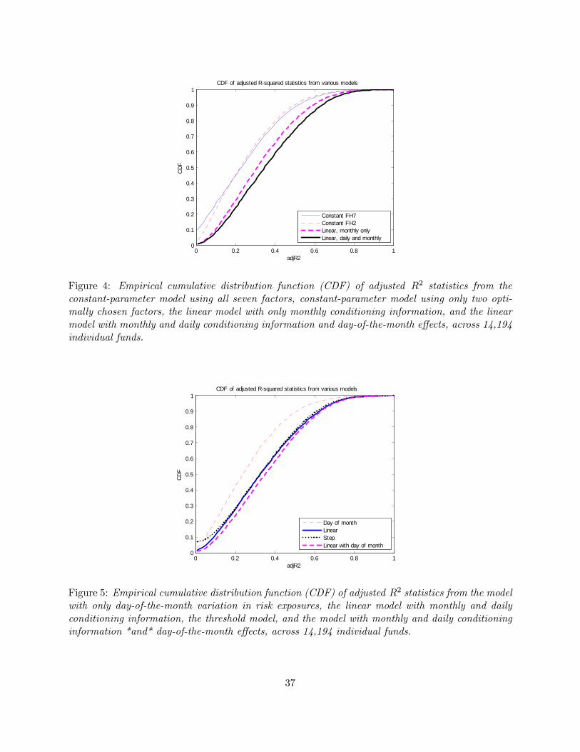
0 0.2 0.4 0.6 0.8 10

0.1

0.2

0.3

0.4

0.5

0.6

0.7

0.8

0.9

1

adjR2

CDF

CDF of adjusted R­squared statistics from various models

Constant FH7Constant FH2Linear, monthly onlyLinear, daily and monthly

Figure 4: Empirical cumulative distribution function (CDF) of adjusted R2 statistics from theconstant-parameter model using all seven factors, constant-parameter model using only two opti-mally chosen factors, the linear model with only monthly conditioning information, and the linearmodel with monthly and daily conditioning information and day-of-the-month e¤ects, across 14,194individual funds.

0 0.2 0.4 0.6 0.8 10

0.1

0.2

0.3

0.4

0.5

0.6

0.7

0.8

0.9

1

adjR2

CDF

CDF of adjusted R­squared statistics from various models

Day of monthLinearStepLinear with day of month

Figure 5: Empirical cumulative distribution function (CDF) of adjusted R2 statistics from the modelwith only day-of-the-month variation in risk exposures, the linear model with monthly and dailyconditioning information, the threshold model, and the model with monthly and daily conditioninginformation *and* day-of-the-month e¤ects, across 14,194 individual funds.

37

0 5 10 15 20 250

0.2

0.4

0.6

0.8

1

1.2

1.4

1.6

1.8

Day of the month

Weig

ht

MIDAS weights on factor

Day­of­Month onlyLinear and Day­of­Month

Figure 6: Day-of-the-month variation in risk exposures from the model with only day-of-the-monthe¤ects, and the model including both day-of-the-month e¤ects and variation in risk exposures thatis linear in both daily and monthly conditioning variables. Sample consists of funds with signi�canttime-variation in risk exposures.

38

39

Table I Summary Statistics

This table shows summary statistics for the funds in our sample. Panel A reports the percentiles of the pooled (cross-sectional) distribution of returns, unsmoothed returns, AUM, management fees, incentive fees, lockup and redemption notice periods. Panel B shows the percentages of funds in the consolidated sample of 14,194 which have return histories of the lengths specified in the column headers. Panel C shows the number and percentage of the 14,194 funds in each of the strategies represented in the rows.

Panel A

Returns Unsmoothed AUM Management Incentive Fee Lockup Redemption Notice

Returns ($MM) Fee Fee (Days) (Days)

25th Prctile -0.700 -0.841 9.400 1.000 10.000 0.000 10.000 50th Prctile 0.720 0.710 32.000 1.500 20.000 0.000 30.000 75th Prctile 2.230 2.363 106.756 2.000 20.000 90.000 45.000 Mean 0.845 0.847 166.714 1.484 15.162 94.176 33.913

Panel B

<36 Months >=36 , <60 >=60

Length(Return History) 17.423 31.062 51.515

Panel C

Funds in Strategy

Percent Number

Security Selection 20.752 2946

Global Macro 6.243 846 Relative Value 1.030 146 Directional Traders 12.788 1815 Funds of Funds 23.341 3313

Multi-Process 12.520 1777

Emerging Markets 3.372 479

Fixed Income 5.678 806 CTAs 13.973 1983 Other 0.303 43

TOTAL 100 14194

40

Table II The Linear Model for Daily and Monthly Hedge Fund Style Indexes

Table II shows results from a two-factor model applied to five hedge fund style index returns, identified in the first row of the table, allowing for time variation in the factor exposures as a linear function of conditioning variables (i.e., g(Z) is linear in Z, as in equation 6). Two factors from the set of four daily Fung-Hsieh factors are selected for each style, using the Bayesian Information Criterion – these are identified in the Internet Appendix. The first row presents annualized alpha. Robust standard errors are reported below the parameter estimates, and the R2 and adjusted R2 are also reported. The fourth-last row presents the p-value for the joint significance of the coefficients on the interaction terms (Gamma1, Gamma2, Delta1, Delta2). The second-last and final rows present the correlation between the time series of daily factor exposures estimated using daily and monthly data, for each of the two factors. For ease of comparison, Z is picked to be dLevel for all indexes.

Equity Hedge Macro Directional Merger Arbitrage Relative Value

Daily Monthly Daily Monthly Daily Monthly Daily Monthly Daily Monthly

alpha 1.406 3.064 3.395 3.200 3.226 7.612 4.792 4.450 0.652 3.980 s.e. 2.217 2.053 3.782 3.859 3.529 3.213 1.417 1.402 2.860 1.820 beta1 0.308 0.327 0.066 0.121 0.318 0.248 0.092 0.104 0.107 0.076 s.e. 0.008 0.051 0.027 0.144 0.012 0.081 0.005 0.035 0.010 0.045 beta2 -1.873 -1.802 -0.748 -0.766 -2.483 -3.293 -0.677 -0.614 -1.900 -5.795 s.e. 0.291 0.698 0.244 1.248 0.470 1.037 0.186 0.477 0.375 0.619 gam1 0.006 0.010 0.001 0.003 0.005 0.002 -0.001 0.009 0.005 -0.010 s.e. 0.001 0.006 0.003 0.025 0.001 0.009 0.000 0.004 0.001 0.005 gam2 -0.009 0.027 0.039 0.069 0.004 -0.025 -0.059 0.027 0.129 0.002 s.e. 0.031 0.113 0.032 0.148 0.048 0.170 0.020 0.077 0.041 0.100 delta1 0.006 0.034 -0.012 -0.022 0.004 0.054 -0.003 -0.003 0.017 0.050 s.e. 0.002 0.012 0.008 0.071 0.003 0.018 0.002 0.008 0.003 0.011 delta2 0.221 0.325 -0.272 1.082 0.295 1.119 -0.006 0.187 0.100 0.099 s.e. 0.072 0.763 0.108 0.763 0.103 1.130 0.046 0.521 0.093 0.676

R2 0.575 0.734 0.019 0.049 0.470 0.715 0.291 0.262 0.131 0.846 R2adj 0.573 0.710 0.016 -0.035 0.468 0.683 0.288 0.197 0.127 0.832

pval 0.000 0.008 0.074 0.557 0.000 0.035 0.010 0.150 0.000 0.000

Corr-b1 0.897 0.985 0.420 -0.492 0.199 Corr-b2 0.911 -0.776 0.992 -0.523 0.352

41

Table III Hedge Fund Time-Varying Risk Exposures: Linear Model

This table shows results from the linear model (i.e., g(Z) is linear in Z, as in equation 6) for time-varying risk exposures in hedge fund returns. The table shows the proportion of 14,194 hedge funds for we can reject the null hypothesis of constant risk exposures at the 5% level of significance, according to various models: the model with both daily and monthly Z variation allowed; the model with only monthly variation in Z; the incremental significance of daily Z variation over and above monthly Z variation; and the incremental significance of monthly Z variation over and above daily Z variation. The column headers list the four Z variables that we consider (the change in the 3-month US T-bill rate (labelled dLevel), S&P 500 returns, exponentially detrended VIX, and the TED spread), followed by a simple average of the proportions across Z variables.

Conditioning Variables

Model dLevel SP500 VIX TED Average

Daily and Monthly 25.673 22.973 21.566 19.281 22.373 Monthly Only 15.393 13.608 9.448 9.531 11.995 Daily Given Monthly 23.018 21.399 23.056 20.870 22.086

Monthly Given Daily 15.325 10.386 13.434 9.947 12.273

42

Table IV Linear Model Results by Hedge Fund Style

This table shows the proportion of hedge funds across the ten styles for which we can reject the null hypothesis of constant risk exposures at the 5% level of significance, using the linear model (i.e., g(Z) is linear in Z, as in equation 6). Panel A shows these results for a model which allows for Z variation at both daily and monthly frequencies, and Panel B shows the proportion of funds for which allowing for daily variation is significant over and above a baseline monthly model. The columns show the four choices of Z considered and the average proportion across all four.

Panel A: Daily and monthly Conditioning Variables

Style N(Funds) dLevel SP500 VIX TED Average

Security Selection 2942 22.175 18.243 16.082 15.409 17.977 Macro 885 14.400 15.333 12.267 11.733 13.433 Relative Value 146 19.118 19.118 20.588 18.382 19.302 Directional Traders 1813 24.563 22.479 16.958 16.789 20.197 Fund of Funds 3309 42.853 36.775 38.853 29.271 36.938 Multi-Process 1775 25.382 23.325 21.915 21.093 22.929 Emerging 478 13.763 19.140 18.065 12.043 15.753 Fixed Income 805 16.255 21.456 13.914 23.667 18.823 CTA 1981 12.171 9.013 9.737 10.132 10.263

Other 43 17.949 12.821 17.949 17.949 16.667

Panel B: Daily given monthly Conditioning Variables

Style N(Funds) dLevel SP500 VIX TED Average

Security Selection 2942 18.101 15.551 17.641 16.082 16.844 Macro 885 11.200 9.467 11.867 11.200 10.933 Relative Value 146 18.382 26.471 20.588 23.529 22.243 Directional Traders 1813 19.493 16.394 18.085 19.268 18.310 Fund of Funds 3309 40.217 35.876 41.178 33.488 37.690 Multi-Process 1775 24.442 24.031 24.266 23.090 23.957 Emerging 478 13.978 15.914 17.204 13.763 15.215 Fixed Income 805 19.766 28.088 16.515 22.887 21.814 CTA 1981 9.145 8.355 10.263 8.421 9.046

Other 43 17.949 12.821 12.821 12.821 14.103

43

Table V Mutual Fund Time-Varying Risk Exposures: Linear Model

This table shows results from the linear model (i.e., g(Z) is linear in Z, as in equation 6) for time-varying risk exposures in mutual fund returns. Panel A (B) of the table shows the proportion of 17,886 “equity” mutual funds in the CRSP database with ≥50% average allocation to common or preferred stocks (15,027 “bond” funds with < 50% average allocation to common or preferred stocks) for we can reject the null hypothesis of constant risk exposures at the 5% level of significance, according to various models: the model with both daily and monthly Z variation allowed; the model with only monthly variation in Z; the incremental significance of daily Z variation over and above monthly Z variation; and the incremental significance of monthly Z variation over and above daily Z variation. The column headers list the four Z variables that we consider (the change in the 3-month US T-bill rate (labelled dLevel), S&P 500 returns, exponentially detrended VIX, and the TED spread), followed by a simple average of the proportions across Z variables. Panel A: Equity Funds Conditioning Variables Model dLevel SP500 VIX TED Average Daily and Monthly 17.685 18.733 7.340 19.537 15.824 Monthly Only 17.492 13.894 9.684 18.228 14.824 Daily Given Monthly 8.941 13.337 4.477 12.013 9.692

Monthly Given Daily 16.633 10.234 5.757 17.720 12.586

Panel B: Bond Funds

Conditioning Variables

Model dLevel SP500 VIX TED Average

Daily and Monthly 13.966 15.756 6.759 13.033 12.379 Monthly Only 12.078 14.899 5.386 12.429 11.198 Daily Given Monthly 10.422 9.719 5.667 10.539 9.087

Monthly Given Daily 10.808 12.049 4.110 14.286 10.313

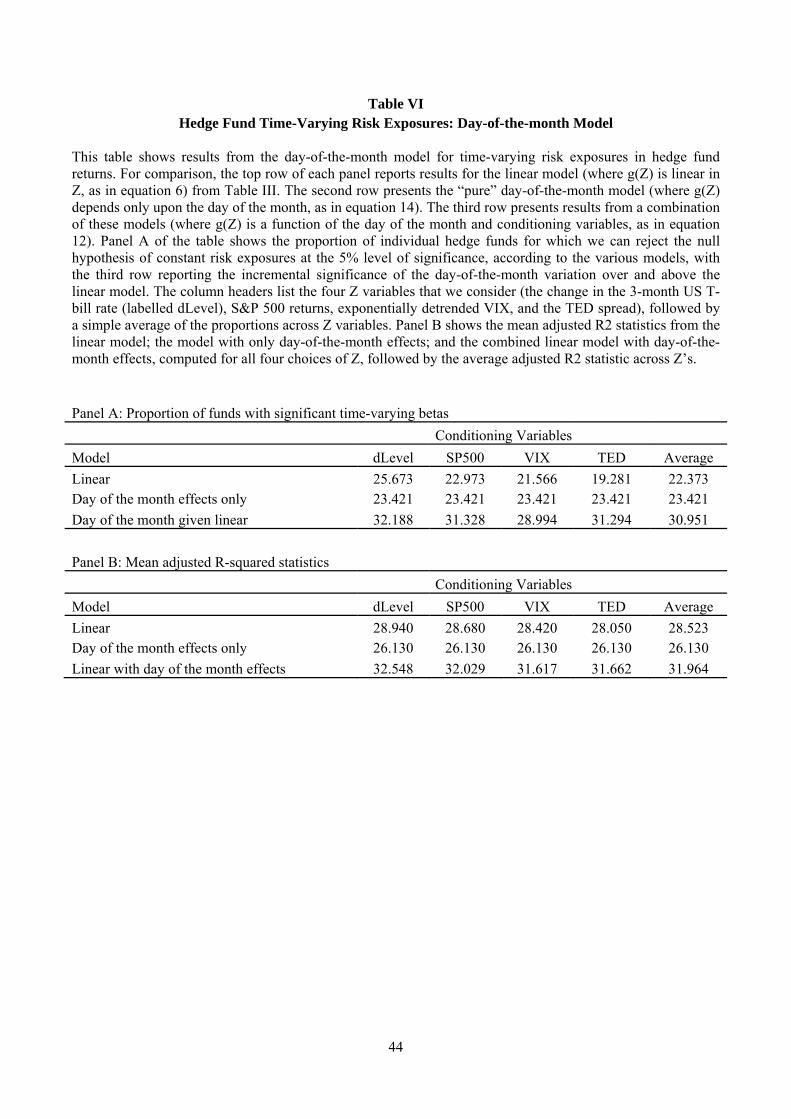
44

Table VI Hedge Fund Time-Varying Risk Exposures: Day-of-the-month Model

This table shows results from the day-of-the-month model for time-varying risk exposures in hedge fund returns. For comparison, the top row of each panel reports results for the linear model (where g(Z) is linear in Z, as in equation 6) from Table III. The second row presents the “pure” day-of-the-month model (where g(Z) depends only upon the day of the month, as in equation 14). The third row presents results from a combination of these models (where g(Z) is a function of the day of the month and conditioning variables, as in equation 12). Panel A of the table shows the proportion of individual hedge funds for which we can reject the null hypothesis of constant risk exposures at the 5% level of significance, according to the various models, with the third row reporting the incremental significance of the day-of-the-month variation over and above the linear model. The column headers list the four Z variables that we consider (the change in the 3-month US T-bill rate (labelled dLevel), S&P 500 returns, exponentially detrended VIX, and the TED spread), followed by a simple average of the proportions across Z variables. Panel B shows the mean adjusted R2 statistics from the linear model; the model with only day-of-the-month effects; and the combined linear model with day-of-the-month effects, computed for all four choices of Z, followed by the average adjusted R2 statistic across Z’s.

Panel A: Proportion of funds with significant time-varying betas

Conditioning Variables

Model dLevel SP500 VIX TED Average

Linear 25.673 22.973 21.566 19.281 22.373 Day of the month effects only 23.421 23.421 23.421 23.421 23.421

Day of the month given linear 32.188 31.328 28.994 31.294 30.951

Panel B: Mean adjusted R-squared statistics

Conditioning Variables

Model dLevel SP500 VIX TED Average

Linear 28.940 28.680 28.420 28.050 28.523 Day of the month effects only 26.130 26.130 26.130 26.130 26.130

Linear with day of the month effects 32.548 32.029 31.617 31.662 31.964

45

Table VII Day-of-the-month Model Results by Hedge Fund Style

This table shows the proportion of individual hedge funds across the ten styles for which we can reject the null hypothesis of day-of-the-month variation in risk exposures at the 5% level of significance. Panel A shows these results for a model which allows for day-of-the-month effects alone (as in equation 14), and Panel B shows these results for the combined linear model with day-of-the-month effects (as in equation 12). The columns show the four choices of Z considered and the average proportion across all four.

Panel A: Day of the month effects only

Style N(funds)

Security Selection 1844 19.089 Macro 561 18.182 Relative Value 87 34.483 Directional Traders 1187 19.377 Fund of Funds 2353 30.472 Multi-Process 1151 26.846 Emerging 293 23.891 Fixed Income 533 26.266 CTA 1212 17.327

Other 18 27.778

Panel B: Linear with day of the month effects Conditioning Variables

Style dLevel SP500 VIX TED Average

Security Selection 24.368 25.828 23.695 22.852 24.186 Macro 25.383 25.602 22.101 23.195 24.070 Relative Value 31.325 31.325 32.530 34.940 32.530 Directional Traders 23.484 23.313 21.435 22.289 22.630 Fund of Funds 47.135 43.056 40.061 48.134 44.597 Multi-Process 34.779 32.430 33.153 31.256 32.905 Emerging 28.322 32.517 21.678 25.874 27.098 Fixed Income 29.377 32.296 25.486 27.043 28.551 CTA 24.236 23.443 23.556 24.575 23.953

Other 23.529 23.529 17.647 35.294 25.000

46

Table VIII Insights from the Threshold Model

This table shows results from the threshold model (where g(Z) is a nonlinear function of Z, as in equation 15, with risk exposures moving abruptly when Z hits a pre-specified threshold value) for time-varying risk exposures in hedge fund returns. The variables Z are named in the first column. The thresholds are quantiles, given in the second column, of the variable’s month-end distribution. The third column of the table shows the proportion of 14,194 hedge funds for we can reject the null hypothesis of constant risk exposures at the 5% level of significance, using this model. The fourth through seventh columns show the factor on which the loading changes according to the threshold model. The first row shows the unconditional average risk exposures to each of the factors. The next four rows show how these risk exposures change when each of the four conditioning variables crosses its threshold, falling below (rising above) the 10th (90th) percentile of its month-end distribution at any point within the month. For example, the average fund’s risk exposure to the S&P 500 falls by 64.4%, and its risk exposure to the credit spread rises (towards zero) by 107.5%, when S&P 500 realized volatility rises above the 90th percentile of its month-end distribution.

% Significant SP500 SMB TCM10Y BAAMTSY

Average Value 0.419 0.233 -1.780 -4.595 Cond. Variable Quantile Percentage changes relative to average risk exposure

dLevel < 0.10 18.700 10.263 -19.742 88.202 45.680 SP 500 Return < 0.10 15.499 -0.716 -126.180 -45.899 -35.930 SP 500 volatility > 0.90 35.000 -64.439 -16.738 72.753 107.552

TED > 0.90 33.400 -52.745 -98.712 77.191 10.381

47

Table IX Accounting for Time-Variation in Factor Exposures: Implications for Alpha

This table presents analysis of the estimated alpha of individual hedge funds using a traditional static model (where risk exposures are assumed constant) presented in the first column, and three different models for time-varying risk exposures: Panel A presents results for the linear model (where g(Z) is linear in Z, as in equation 6); Panel B presents results for the linear model with day-of-the-month effects (where g(Z) is linear in Z and also includes a deterministic day-of-the-month effect, as in equation 12); Panel C presents results for the threshold model (where g(Z) is a nonlinear function of Z, as in equation 15, with risk exposures moving abruptly when Z hits a pre-specified threshold value). The first two columns present annualized means of the estimated alphas from different models. The third column shows the cross-sectional mean difference between the dynamic model alpha and the static model alpha, the fourth column reports the cross-sectional mean of the absolute value of the difference of these alphas, and the final column reports the cross-sectional rank correlation of these alphas. Within each panel we present results separately for all funds, or only funds for which we can reject the null hypothesis of constant risk exposures. Note that the model in Panel B requires more time series observations, and so the universe of funds considered there is smaller than in Panels A and C (9,239 compared with 14,194 funds) and thus the results for the static model are different in that panel than the other two panels.

Mean Alpha Mean Alpha Difference |Difference| Rank

Static model

(1) T-V beta model

(2) Correlation

Panel A: Linear model All funds 4.173 5.066 -0.893 3.170 0.868

t-stat 40.683 46.089 -16.733 67.635 60.964

Funds w/sig. variation 3.677 5.105 -1.428 3.497 0.806

t-stat 28.905 35.398 -17.478 49.191 55.928 Panel B: Linear model with Day-of-the-Month effects All funds 4.331 5.035 -0.704 2.730 0.857

t-stat 44.662 48.644 -13.935 65.328 113.949

Funds w/sig. variation 3.818 4.852 -1.034 2.790 0.817

t-stat 32.667 38.270 -15.020 49.056 67.419

Panel C: Threshold model All funds 4.173 3.981 0.192 4.656 0.692

t-stat 40.683 35.452 2.292 62.729 40.036

Funds w/sig. variation 3.677 3.920 -0.243 4.189 0.674

t-stat 28.905 26.419 -2.027 38.957 20.602

48

Table X Understanding the Sources of Time-Variation in Risk Exposures

This table decomposes the variation in betas for a set of 252 management companies. These companies run all the long/short equity hedge funds reporting quarterly 13-F filings information on their portfolio holdings which matched our consolidated dataset of hedge funds. The variation in total beta (estimated by applying reported stock-level weights from the 13-Fs to stock-level time-varying betas) is split into four components, namely: pure weight variation (variation in portfolio weights holding underlying asset betas constant); pure beta variation (variation in underlying asset betas holding portfolio weights constant); weight-beta variation (arising from the co-variation between weights and betas); and a covariance term representing the difference between total beta variation and the sum of these three components, as in equation 19. Each column of the table reports the cross-sectional average variance of each of these components expressed as a fraction of the total variation in fund beta, with the associated White heteroskedasticity-robust t-statistic reported below each number. The rows represent the variable used to estimate time-varying underlying asset beta (at the quarterly frequency) in each case, namely the change in the 3-month US T-bill rate (labelled dLevel), S&P 500 returns, the first difference of VIX, and the quarterly change in the TED spread.

Panel A: Full sample

Pure Pure Weight Cov.

weight beta ×beta terms

dLevel 56.963 33.014 17.013 -6.991 t-stat 33.107 20.577 20.702 -3.352 SP500 79.606 9.848 18.560 -8.014 t-stat 38.087 8.696 17.493 -4.046 VIX 81.516 8.260 9.963 0.262 t-stat 58.984 8.878 13.448 0.239 dTED 72.902 15.321 18.221 -6.444 t-stat 41.099 7.677 13.863 -2.322

Average 72.747 16.611 15.939 -5.297

Panel B: Credit crisis (2007-2010)

Pure Pure Weight Cov.

weight beta ×beta terms

dLevel 92.500 19.940 26.540 -38.980 t-stat 13.601 7.373 10.225 -4.584 SP500 82.506 18.330 23.383 -24.219 t-stat 28.064 8.101 8.854 -5.641 VIX 81.527 17.009 23.048 -21.584 t-stat 29.280 7.815 8.329 -5.322 dTED 79.946 17.681 25.357 -22.985 t-stat 30.457 7.202 8.289 -4.714

Average 84.120 18.240 24.582 -26.942

1

Internet Appendix for

“On the High Frequency Dynamics of

Hedge Fund Risk Exposures”

This internet appendix provides supplemental analyses to the main tables in “On the High Frequency Dynamics of Hedge Fund Risk Exposures”

The first section describes the process used to create the consolidated database of hedge funds that is employed in this paper from the TASS, HFR, MSCI and CISDM databases. Prior to Table IA.IV, we describe the simulation, and prior to Table IA.V, we describe the robustness checks conducted in that table. The tables and figures are as follows:

Table IA.I: Summary Statistics on Funds in Consolidated Database

Table IA.II: Static Factor Models for Daily and Monthly Hedge Fund Style Indexes

Table IA.III: Comparison of results based on simple and log returns Table IA.IV: Results from a simulation study of the estimation method

Table IA.V: Robustness checks

Figure IA.1: Static factors selected by strategy

Figure IA.2: Some possible shapes with exponential-Almon weight functions

2

The Consolidated Hedge Fund Database

As hedge funds can report to one or more databases, the use of any single source will fail to capture the complete universe of hedge fund data. We therefore aggregate data from TASS, HFR, CISDM, BarclayHedge and Morningstar, which together have 48,508 records that comprise administrative information as well as returns and AUM data for hedge funds, fund of funds and CTAs. However this number hides the fact that there is significant duplication of information, as multiple providers often cover the same fund. To identify all unique entities, we must therefore consolidate the aggregated data. To do so, we adopt the following steps: 1. Group the Data: Records are grouped based on reported management company names. To do so, we first create a `Fund name key' and a `Management company key' for each data record, by parsing the original fund name and management company name for punctuations, filler words (e.g., `Fund', `Class'), and spelling errors. We then combine the fund and management name keys into 4,409 management company groups. 2. De-Duplication: Within a management company group, records are compared based on returns data (converted into US dollars), and 18,130 match sets are created out of matching records, allowing for a small error tolerance limit (10% deviation) to allow for data reporting errors. 3. Selection: Once all matches within all management company groups are identified, a single record representing the unique underlying fund is created for each match set. We pick the record with the longest returns data history available is selected from the match set, and fill in any missing administrative information using the remaining records in the match set. The process thus yields 18,130 representative fund records. Finally, we apply the criterion that 24 contiguous months of return data are available for each of the funds in the sample we use in the paper. This brings the final number of funds in the sample to 14,194. Table IA.I below shows the number of these final funds from each of the five sources (HFR, TASS, CISDM, MSCI and BarclayHedge), and the number of these funds that are alive and defunct (either liquidated or closed).

3

Table IA.I

Data Sources

This table shows the number of funds from each of the five sources (HFR, TASS, CISDM, MSCI and BarclayHedge), and the number of these funds that are alive and defunct (either liquidated or closed) in the consolidated universe of hedge fund data.

Source Dataset Number of Funds Alive Defunct % Defunct

TASS 5962 2738 3224 54.076 HFR 3712 2449 1263 34.025 CISDM 2782 860 1922 69.087 BarclayHedge 966 930 36 3.727 Morningstar 772 681 91 11.788 Total 14194 7658 6536 46.048

4

Table IA.II Static Factor Models for Daily and Monthly Hedge Fund Style Indexes

This table shows results from a simple two-factor model applied to five hedge fund style index returns, identified in the first row of the table. In all cases a constant is included, and two factors from the set of four daily Fung-Hsieh factors are selected using the Bayesian Information Criterion. The first row presents annualized alpha. Robust t-statistics are reported below the parameter estimates, and the R2 and adjusted R2 are reported in the bottom two rows of the table.

Equity Hedge Macro Directional Merger Arbitrage Relative Value

Daily Monthly Daily Monthly Daily Monthly Daily Monthly Daily Monthly

Alpha 1.575 1.595 3.738 3.322 3.044 3.709 5.444 5.331 -1.032 -0.473 t-stat 0.781 0.880 0.985 0.985 0.995 1.453 3.376 4.208 -0.422 -0.234 SP500 0.259 0.321 0.270 0.327 0.111 0.063 0.063 0.190 t-stat 15.395 6.070 11.298 4.029 5.181 2.332 1.811 3.935 SMB 0.070 0.111 t-stat 2.111 0.849 TCM10Y -0.905 -0.376 t-stat -2.742 -0.405 BAAMTSY -2.006 -2.027 -2.720 -3.861 -0.460 -0.579 -2.544 -6.080

t-stat -4.184 -2.728 -3.847 -3.686 -0.804 -1.935 -3.724 -9.584

R2 0.549 0.681 0.014 0.007 0.454 0.664 0.290 0.182 0.090 0.784

R2adj 0.548 0.672 0.013 -0.021 0.453 0.652 0.289 0.160 0.089 0.778

5

Table IA.III Comparison of results based on simple and log returns

This table reports the results from the estimation of the linear model for hedge fund risk exposures, described in Section 2.2.1, and can be compared with the results presented in Table II of the paper. The columns labeled “True” are based on daily simple returns that are compounded to compute monthly simple returns. The columns labeled “Approx” use simple returns but ignore compounding when computing monthly returns. The columns labeled “Log” are based on log returns, which cumulated to monthly returns exactly, but render the factor model only approximate.

                                                        

Equity Hedge Macro Directional Merger Arbitrage Relative Value

True Approx Log True Approx Log True Approx Log True Approx Log True Approx Log

alpha 3.127 3.187 3.064 3.586 3.452 3.200 7.702 7.778 7.612 4.494 4.462 4.450 3.891 4.006 3.980

s.e. 2.058 2.051 2.053 3.864 3.839 3.859 3.230 3.206 3.213 1.404 1.396 1.402 1.817 1.818 1.820

beta1 0.328 0.326 0.327 0.125 0.123 0.121 0.250 0.248 0.248 0.104 0.104 0.104 0.076 0.076 0.076

s.e. 0.051 0.051 0.051 0.145 0.144 0.144 0.082 0.081 0.081 0.035 0.034 0.035 0.045 0.045 0.045

beta2 -1.732 -1.761 -1.802 -0.829 -0.810 -0.766 -3.202 -3.239 -3.293 -0.617 -0.592 -0.614 -5.718 -5.750 -5.795

s.e. 0.698 0.695 0.698 1.255 1.247 1.248 1.040 1.032 1.037 0.476 0.473 0.477 0.616 0.616 0.619

gam1 0.010 0.010 0.010 0.001 0.002 0.003 0.003 0.002 0.002 0.009 0.009 0.009 -0.010 -0.010 -0.010

s.e. 0.006 0.006 0.006 0.025 0.025 0.025 0.009 0.009 0.009 0.004 0.004 0.004 0.005 0.005 0.005

gam2 0.027 0.023 0.027 0.075 0.071 0.069 -0.025 -0.028 -0.025 0.028 0.029 0.027 -0.014 -0.004 0.002

s.e. 0.113 0.112 0.113 0.150 0.149 0.148 0.170 0.169 0.170 0.077 0.076 0.077 0.100 0.100 0.100

delta1 0.031 0.033 0.034 -0.024 -0.024 -0.022 0.051 0.054 0.054 -0.003 -0.004 -0.003 0.047 0.050 0.050

s.e. 0.012 0.012 0.012 0.073 0.073 0.071 0.018 0.018 0.018 0.008 0.008 0.008 0.011 0.011 0.011

delta2 0.200 0.280 0.325 1.128 1.103 1.082 0.877 1.040 1.119 0.200 0.128 0.187 -0.084 0.007 0.099

s.e. 0.791 0.788 0.763 0.776 0.771 0.763 1.176 1.167 1.130 0.539 0.536 0.521 0.698 0.698 0.676

R2 0.723 0.730 0.734 0.049 0.049 0.049 0.696 0.710 0.715 0.262 0.250 0.262 0.834 0.843 0.846

R2adj 0.699 0.706 0.710 -0.034 -0.035 -0.035 0.661 0.677 0.683 0.197 0.183 0.197 0.820 0.829 0.832

pval 0.012 0.010 0.008 0.551 0.558 0.557 0.068 0.043 0.035 0.146 0.122 0.150 0.000 0.000 0.000

Simulation Study

We consider a simulation study designed to further investigate the accuracy of our proposed estimation

method. For simplicity, we consider a one-factor model for a hypothetical hedge fund, and as in our main

empirical analysis, we allow factor exposures to vary at both the daily and monthly frequencies. We simplify

the notation and assume that each month contains exactly 22 trading days. This yields a process for daily

hedge fund returns as:

r�d = �+ �f�d + f

�dZd�1 + �f

�dZ

�d�1 + "

�R;d; d = 1; 2; :::; 22� T; (1)

The parameter � captures the average level of beta for this fund, captures variations in beta that are

attributable to the monthly variable Zd; and � captures variations in beta that are attributable to the daily

variable Z�d : If we aggregate this process up to the monthly frequency we obtain:

rt = 22�+ �ft + ftZt�1 + �21Xj=0

f�22t�jZ�22t�j�1 + "R;t; t = 1; 2; :::; T: (2)

where rt �X21

j=0r�22t�j ; is the monthly equivalent of the daily variable in the above speci�cation, and

analogously for ft and Zt. The parameters �; � and are all estimable using only monthly data; the focus

of this simulation study is our ability to estimate �; and whether attempting to do so adversely a¤ects our

estimates of the remaining parameters.

We next specify the dynamics and distribution of the factor and the conditioning variable. To allow for

autocorrelation in the conditioning variable (as found in such variables as volatility and turnover) we use an

AR(1) process for Z�d :

Z�d = �ZZ�d�1 + "

�Z;d

The conditioning variable is de-meaned prior to estimation, and so the omission of an intercept in the above

speci�cation is without loss of generality. We also assume an AR(1) for the factor returns, to allow for the

possibility that these are also autocorrelated:

f�d = �F + �F�f�d�1 � �F

�+ "�F;d

Finally, we assume that all innovations are normally distributed, and we allow for correlation between the

factor innovations and the innovations to the conditioning variable:

�"�R;d; "

�F;d; "

�Z;d

�0 s N0BBB@266640

0

0

37775 ;26664�2"R 0 0

� �2"F �FZ�"F�"Z

� � �2"Z

377751CCCA

To obtain realistic parameter values for the simulation we calibrate the model to the results obtained when

estimating the model using daily HFR equity hedge index returns. This leads to the following parameters

6

for our simulation:

� = 2=(22� 12); � = 0:4; = 0:002; � = �0:004

�F = 10= (22� 12) ; �F = 20=p22� 12; �Z = 10; �"R =

p0:1

Thus we assume that the fund generates 2% alpha per annum with an average beta of 0.4, and a daily beta

that varies with both daily and monthly �uctuations in the conditioning variable (Z� and Z). The factor

is assumed to have an average return of 10% per annum and an annual standard deviation of 20%. The

conditioning variable has daily standard deviation of 10 (similar to the VIX), and the innovation to the

returns process has a daily variance of 0.1, which corresponds to an R2 of around 0.6 in this design.

We vary the other parameters of the returns generating process in order to study the sensitivity of the

method to these parameters. We consider:

�Z 2 f0; 0:5; 0:9g ; �F 2 f�0:2; 0; 0:2g ; �FZ 2 f0; 0:5g ; T 2 f24; 60; 120g

Thus, we allow the conditioning variable to vary from iid (�Z = 0) to persistent (�Z = 0:9); we allow for

moderate negative or positive autocorrelation in the factor returns; we allow for zero or positive correlation

between the factor and the conditioning variable; and we consider three sample sizes: 24 months, 60 months

or 120 months, which covers the relevant range of sample sizes in our empirical analysis (the average sample

size in our empirical application is 62 months). We simulate each con�guration of parameters 1000 times,

and report the results in Table IA.IV.

The results show that the estimation method proposed in the paper performs very well in all the scenarios

that we consider. In the �base� scenario, even with just 60 months of data we are able to reasonably

accurately estimate the parameters of this model, including the parameter �, which allows us to capture daily

variation in hedge fund risk exposures. Across a range of di¤erent sample sizes, degrees of autocorrelation,

and correlation with the factor return, the estimation method performs well: the 90% con�dence interval of

the distribution of parameter estimates contains the true parameter in all ten scenarios that we consider.

7

8

Table IA.IV Results from a simulation study of the estimation method

This table reports the mean and standard deviation, across 1000 independent simulation replications, of estimates of the parameters of a model of time-varying factor exposures. The results for ten different simulation designs are presented. Simulation design parameters are presented in the first panel of the table, and the mean and standard deviation of the simulation distribution of parameter estimates are presented in the second and third panels. The true values of the four parameters are presented in the first column of the table. The values for alpha, gamma and delta are scaled up by a factor of 100 for ease of interpretability.

1 2 3 4 5 6 7 8 9 10

True

values Base

scenario Short

sample Long

sample

Low autocorr

in Z

High autocorr

in Z

Corr b/w F,

Z

Neg autocorr

in F, rhoFZ=0

Pos autocorr

in F, rhoFZ=0

Neg autocorr

in F, rhoFZ=0.5

Pos autocorr

in F, rhoFZ=0.5

T 60 24 120 60 60 60 60 60 60 60 rhoFZ 0.0 0.0 0.0 0.0 0.0 0.5 0.0 0.0 0.5 0.5 phiZ 0.5 0.5 0.5 0.0 0.9 0.5 0.5 0.5 0.5 0.5 phiF 0.0 0.0 0.0 0.0 0.0 0.0 -0.2 0.2 -0.2 0.2

Mean Alpha*100 0.758 0.715 0.827 0.794 0.729 0.773 0.812 0.780 0.735 0.725 0.721 Mean Beta 0.400 0.400 0.397 0.399 0.400 0.401 0.400 0.401 0.400 0.399 0.401 Mean Gamma*100 0.200 0.198 0.198 0.200 0.198 0.200 0.200 0.199 0.201 0.198 0.199 Mean Delta*100 -0.400 -0.391 -0.400 -0.409 -0.399 -0.404 -0.410 -0.381 -0.392 -0.397 -0.394

St dev Alpha*100 0.089 0.146 0.062 0.089 0.092 0.194 0.085 0.091 0.191 0.191 St dev Beta 0.035 0.060 0.024 0.033 0.035 0.035 0.042 0.031 0.041 0.029 St dev Gamma*100 0.005 0.009 0.003 0.008 0.003 0.005 0.006 0.004 0.005 0.004 St dev Delta*100 0.038 0.062 0.026 0.035 0.052 0.034 0.039 0.034 0.037 0.031

9

Robustness Checks Table IA.V presents robustness checks used to identify whether the method proposed in this paper performs well over different sample periods, over different samples of funds, and under different transformations of hedge fund returns. In all these robustness checks, we consider the linear model for g(Z), and use dLevel as Z. We consider a model using both daily and monthly conditioning information, as well as a model based only on monthly information. The first robustness check that we run is to split the sample period into two halves, with the second half beginning in 2002, after the NASDAQ crash, and extending up to 2009, including the credit crisis period. We find that our method performs relatively less well in the early period, with 14.2% of funds rejecting the null of no significant interaction variables. In the second sub-period, we find almost 30% of the funds selecting interactions. This might be explained by the population of funds shifting towards funds with faster-moving trading strategies, which would suggest that our method is more appropriate to use in the contemporary setting. The model using only monthly information performs equally well in both sub-periods. Next, we investigate our use of the Getmansky, Lo and Makarov (2004) unsmoothing of hedge fund returns. Our baseline results us 2 lags when implementing this model, and we find that our results are essentially unaffected by the choice of using more lags (4) or no lags. We then condition on the length of available return history for the funds, and find that the both models perform better for funds with longer return histories, which is understandable given that it gives us more information with which to pick up changes in risk exposures. Finally, we condition on the size of the fund. We find that both methods work better for larger hedge funds (measured by the average AUM over the fund's lifetime), and worse for funds in the smallest tercile of AUM.

10

Table IA.V Robustness Checks

This table presents the proportion of funds with significant time variation based on our linear model (g(Z) linear in Z, allowing for both daily and monthly variation in Z; or only monthly variation in Z), using dLevel as Z. These proportions selected change when the specification is altered according to the robustness checks itemized in the rows of the first column. The first row is taken from the main table of linear model results (Table III) and is repeated here for ease of reference. The first set of robustness checks splits the sample period into two halves; the second set alters the type of “unsmoothing” done to the returns prior to testing; the third set sorts funds according to their history lengths in the consolidated database; and the fourth set sorts funds according to their average assets under management.

Robustness Test N(Funds) Daily and Only

Monthly Monthly

Main Results in Paper 14194 25.673 15.393 Sample Period Earlier period (1994:01-2001:12) 5106 14.219 14.044 Later period (2002:01-2009:06) 11386 29.832 15.168 Smoothing Raw returns (no GLM) 14194 24.600 13.800 Longer (4) MA lags in GLM model 14194 24.700 16.300 Fund History Length 24<=N(Fund Observations)<36 2697 13.200 7.379 36<=N(Fund Observations)<60 4394 20.096 11.174 N(Fund Observations)>=60 7103 31.635 20.301 Fund Size Avg AUM <= 33rd Prctile 3963 15.821 11.380 33rd Prctile< Avg AUM <= 66th Prctile 4085 24.357 16.010

Avg AUM > 66th Prctile 3963 32.677 18.193

11

Figure IA.1: Static factors selected by strategy

12

Figure IA.2: Some possible shapes with exponential-Almon weight functions