Embed Size (px)
Citation preview

Biological Science – Neuroscience / Physical Sciences – Applied Mathematics
Optimal Population Coding, Revisited
Philipp Berens1,2,3,4, Alexander S. Ecker1,2,3,4, Sebastian Gerwinn1,2,3, Andreas S. Tolias1,4,5,6, Matthias
Bethge1,2,3
1. Bernstein Centre for Computational Neuroscience Tübingen, Spemannstr. 41, 72076 Tübingen, Germany
2. Werner Reichardt Centre for Integrative Neuroscience and Institute of Theoretical Physics, University of Tübingen, 72076 Tübingen, Germany
3. Max Planck Institute for Biological Cybernetics, Computational Vision and Neuroscience Group, Spemannstr. 41, 72076 Tübingen, Germany
4. Baylor College of Medicine, Department of Neuroscience, One Baylor Plaza, Houston, TX 77030, USA
5. Michael E. DeBakey Veterans Affairs Medical Center, Houston, TX, USA
6. Department of Computational and Applied Mathematics, Rice University, Houston, TX 77005, USA.
Corresponding author:
Philipp Berens
Max Planck Institute for Biological Cybernetics
Computational Vision and Neuroscience
Spemannstr. 41
72076 Tübingen
Email: [email protected]
Phone: +49-7071-6011775
Fax: +49-3212-12 44 313
Keywords:
Population Coding, Fisher information, Discrimination Error, Tuning Width, Noise Correlation

Abstract
Cortical circuits perform the computations underlying rapid perceptual decisions within a few dozen
milliseconds with each neuron emitting only a few spikes. Under these conditions, the theoretical analysis
of neural population codes is challenging, as the most commonly used theoretical tool – Fisher
information – can lead to erroneous conclusions about the optimality of different coding schemes. Here
we revisit the effect of tuning function width and correlation structure on neural population codes based
on ideal observer analysis in both a discrimination and reconstruction task. We show that the optimal
tuning function width and the optimal correlation structure in both paradigms strongly depend on the
available decoding time in a very similar way. In contrast, population codes optimized for Fisher
information do not depend on decoding time and are severely suboptimal when only few spikes are
available. In addition, we use the neurometric functions of the ideal observer in the classification task to
investigate the differential coding properties of these Fisher-optimal codes for fine and coarse
discrimination. We find that the discrimination error for these codes does not decrease to zero with
increasing population size, even in simple coarse discrimination tasks. Our results suggest that quite
different population codes may be optimal for rapid decoding in cortical computations than those inferred
from the optimization of Fisher information.

Introduction
Neuronal ensembles transmit information through their joint firing rate patterns (1). This raises
challenging theoretical questions on how the encoding accuracy of such population codes is affected by
properties of individual neurons and correlations among them. Any answer to these questions necessarily
depends on the measure used to compare the performance of different population codes. A principled
approach to define such a measure is to use the concept of a Bayesian ideal observer (2, 3). This concept
requires choosing a specific task: in a stimulus reconstruction task, we ask how well a Bayes-optimal
decoder can estimate the true value of the presented stimulus based on the noisy neural response (Fig.
1A). In a stimulus discrimination task, we ask how well it is able to decide which of two stimuli was
presented based on the response pattern (Fig. 1B).
Most theoretical studies of neural coding (4-12) have chosen the stimulus reconstruction paradigm. For
the sake of simplicity and analytical tractability, these studies have evaluated population codes almost
exclusively with regard to Fisher information, assuming its inverse approximates the average
reconstruction error of an ideal observer, the minimum mean squared error. Others have chosen the
stimulus discrimination paradigm, linking Fisher information to the discriminability between two stimuli,
given the neural responses (4, 13-15). In addition to this large body of theoretical work, many
experimental studies have used Fisher information to interpret their results (16-19).
The relationship between Fisher information and the error of an ideal observer in a reconstruction task has
mostly been justified using the Cramér-Rao bound, which states that the conditional mean squared error
of an unbiased estimator of a stimulus is bounded from below by the inverse of the Fisher information
:
(1)
More precisely, this argument is based on the fact that under certain assumptions the maximum a
posteriori estimator is asymptotically normally distributed around the true stimulus with variance equal to
the Cramér-Rao bound (4, 20, 21). Alternatively, using Fisher information to approximate the error of an
ideal observer in a stimulus discrimination task has been justified by noting that the just noticeable
distance is approximately proportional to the inverse square root of the Fisher information (4). The proof
of this relationship similarly relies on a Gaussian approximation of the posterior distribution.
While it is usually taken for granted that Fisher information is an accurate tool for the evaluation and
comparison of population codes, the examples studied by Bethge et al. (20) suggest that the assumptions

necessary to relate Fisher information to the error in the reconstruction or the discrimination task may be
violated in interesting population coding scenarios. In particular, this seems to be the case when the codes
are optimized for Fisher information and the signal-to-noise ratio for individual neurons is low – that is,
exactly in the regime in which neural circuits frequently operate: Perceptual decisions can be made
in less than 100 ms (22), possibly within 30-50 ms (23) and firing rates in cortex are often low (16, 24,
25), such that neural circuits compute with a few spikes at best. In this regime, Fisher information may
yield an incorrect assessment of optimal reconstruction and discrimination performance. Although it is
known in principle that this failure of Fisher information results from its locality, the precise factors that
determine when the validity of Fisher information breaks down are often complex.
To achieve a more precise understanding of this problem we applied a new approach to the investigation
of neural population codes by computing the full neurometric function of an ideal observer in the stimulus
discrimination paradigm (26). A neurometric function shows how the discrimination error achieved by a
population code depends on the difference between the two stimuli. We use it to revisit the question of
optimal population coding with two goals: First, we show that optimal discrimination and optimal
reconstruction lead to qualitatively similar results regarding the effect of tuning function width and of
different noise correlation structures on coding accuracy; in contrast, Fisher information favors coding
schemes which are severely suboptimal for both reconstruction and discrimination at low signal-to-noise
ratio. Second, we use the diagnostic insights provided by neurometric functions in a discrimination task to
obtain an analytical understanding of the poor performance of Fisher-optimal population codes. In
particular, we show that the tuning functions and correlation structures favored by Fisher information
show strikingly bad performance in simple coarse discrimination tasks.
Results
Studying neural population codes using neurometric functions
We obtain neurometric functions by fixing one reference stimulus at orientation , varying the second
stimulus and then plotting the error of the ideal observer trying to discriminate the two based on their
neural representation as a function of their difference (schematically illustrated in Fig. 1C). This graph
contains information about the performance of the population code both in fine and coarse discrimination
tasks.
The ideal observer in such a discrimination task is the Bayes classifier (27)
(2)

where is the population response, the stimulus and . This equation means that
based on the stimulus conditional response distributions the classifier chooses the class which was more
likely to have caused the observed response pattern. As an illustration, consider a single neuron with a
Gaussian response distribution, for which the mean of the response distribution increases from stimulus 1
to stimulus 2 (Fig. 1D). Because of the classification rule, the response will be classified as being caused
by stimulus 2 whenever the neuron responds with a firing rate larger than a certain threshold (dashed line)
even if it was caused by stimulus 1. Therefore, the error of the ideal observer, the minimum
discrimination error (MDE), corresponds to the grey area under the lower of the two probability densities.
Its error is given by (27)
(3)
In general, the classifier achieving the MDE can have a complex shape, reflecting the equal probability
contours of the response distributions. For a population with Gaussian response distributions, the optimal
classifier is linear if the covariance matrix is the same for both stimuli (Fig. 1E), and quadratic, if the
covariance matrices are different (Fig. 1F). Equation (3) can be computed analytically in the linear case.
In the general case, we are still able to evaluate it efficiently even for relatively large populations with
several hundreds of neurons using Monte-Carlo techniques (see Materials and Methods and SI Methods
2). As a measure of the overall performance of a population code we compute the integrated minimum
discrimination error (IMDE), the average performance over all possible discrimination angles (see
Materials and Methods, eq. (9)).
In addition to the minimum discrimination error, we compute the minimum mean squared error (MMSE)
and the Fisher information (see Materials and Methods, eqs. (10) and (11)). The latter yields the
minimum asymptotic error (MASE), the approximation of the MMSE obtained from averaging over the
Cramér-Rao bound (20):
(4)
In the case of asymptotic normality, the MASE yields a good approximation for the MMSE. For a
summary of the acronyms we use to refer to the different coding measures, see table 1.
Optimal tuning function width for individual neurons
For all three measures (MASE, MMSE and IMDE), we investigate how the coding quality of a population
with 100 independent neurons with bell-shaped tuning functions depends on the tuning width of
individual neurons at different time intervals available for decoding (10, 100, 500 and 1000 ms). The

population activity is assumed to follow a multivariate Gaussian distribution with Poisson-like noise,
where variances are identical to mean spike counts (see Materials and Methods). In this model, the signal-
to-noise ratio per neuron increases with the expected spike count, which depends on both the average
firing rates as specified by the tuning functions and the observation time. Here, we only vary the
observation time, which is linearly related to the single neuron signal-to-noise ratio (see Materials and
Methods, eq. (8)).
We first study the effect of tuning width on the coding accuracy in the reconstruction task. We compute
the MASE based on Fisher information as an approximation to the MMSE. According to this measure,
narrow tuning functions are advantageous over broad tuning functions independent of the length of the
time interval used for decoding (Fig. 2A and Fig. S1A and B) as has been reported before (e. g. 9-11). For
the reason of the slight time dependence of the Fisher-optimal tuning width, see Fig. S2. In striking
contrast, numerical evaluation of the MMSE reveals that the optimal tuning width critically depends on
the available decoding time, confirming results of earlier studies (20, 28): for short times, broad tuning
functions were advantageous over narrow ones (Fig. 2B and Fig. S1C and D).
We next evaluate the effect of tuning width in the discrimination paradigm by computing the average
error of an ideal observer, the IMDE. We find that the optimal tuning width in terms of discrimination
error depends on decoding time as well (Fig. 2C): Wide tuning functions are preferable for short and
narrow ones for long integration times (Fig. S1E and F). Despite the fact that the IMDE measures optimal
discrimination and the MMSE-optimal reconstruction performance, the dependence of the IMDE on
tuning width is very similar to that of the MMSE (compare Fig. 2B and C) with IMDE-optimal tuning
curves being only slightly narrower than MMSE-optimal ones. For short integration times, Fisher
information thus failed to reflect the effect of tuning width on coding performance both in the
reconstruction and the discrimination task. These results also hold in the case of discrete Poisson noise
and for Fano factors different than one (Fig. S3).
Neurometric functions allow us to analyze the difference between the results based on Fisher information
and the ideal observer analysis (MMSE and IMDE) in more detail. To do so, we compute the neurometric
functions for populations with Fisher-, MMSE- and IMDE-optimal tuning functions when decoding time
is short (T = 10 ms; Fig. 2D). We find that Fisher-optimal tuning functions are advantageous in fine
discrimination over the tuning functions optimal for the ideal observers, while their performance levels
off for larger at a non-zero error. The neurometric functions computed for populations with MMSE-
and IMDE-optimal tuning width do not show this saturation behavior.
To explain this striking discrepancy, we investigate the coding properties of a population with Fisher-
optimal tuning functions systematically. We compute the Fisher-optimal tuning width for populations of

different size at different integration times (see Materials and Methods) and find that the Fisher-optimal
tuning width is inversely proportional to the population size (Fig. 3A). While Fisher information suggests
that the error achieved by these populations should decay like 1/N as a function of the population size for
all time windows considered (Fig. 3B), the ideal observer error (IMDE) for the same populations saturates
with increasing population size so that adding more neurons does not improve the quality of the code
(Fig. 3C).
The reason for the observed saturation is that the neurometric functions of populations with different size
asymptote at a ‘pedestal error’ P (Fig. 3D). We can provide a lower bound for this pedestal error using the
MDE of an auxiliary population of neurons with additive instead of Poisson-like noise. In this way we
show that the pedestal error is non-zero for finite T and bounded from below by (see SI Text for formal
treatment)
(5)
Here, determines the baseline firing rate, sets the gain of the tuning function and is a constant
independent of N. is the cumulative normal distribution function. Thus the pedestal error does not
decay with increasing population size but is determined by the available decoding time alone, in
agreement with our numerical results (Fig. 3E and F). Intuitively, this is because in Fisher-optimal codes
the tuning width is inversely proportional to N, such that only three cells are active for each stimulus,
independent of N (Fig. 3G). For coarse discrimination, the two stimuli activate two disjoint groups of
neurons (Fig. 3H, red and green neurons). Thus, the error in discriminating two orientations far away
from each other (the pedestal error) is determined solely by the ability to determine which of these two
groups of three neurons is active in the presence of background noise. Using this argument we obtain a
linear approximation of the pedestal error, which has a similar form as eq. (5) (Fig. 3F and SI Text, eq. 2).
In contrast, if the two orientations are very close, the sets of activated neurons overlap and classification
is more difficult (Fig. 3H, red and blue neurons). As can be seen in Fig. 3H, the point at which the
neurometric function reaches its saturation level is approximately twice the difference of the preferred
orientation of two adjacent neurons ( ), independent of the population size (Fig. S4). As the population
size increases, goes to zero and, consequently, as well (Fig. 3I; see SI Text).
Together, these results explain why Fisher-optimal tuning widths lead to saturation of the ideal observer
performance in the large N limit. The IMDE is determined by the area of the initial region of the
neurometric function and the pedestal error P (Fig. 3J):

For fixed T, the pedestal error is independent of N. In contrast, shrinks towards zero with N, because
goes to zero. In the large N limit, the IMDE therefore converges to the pedestal error. To complete
the picture, we note that for fixed N, the pedestal error converges to zero in the large T limit, such that
eventually . Here, Fisher information, which is related to (26), and the IMDE will lead to
similar conclusions.
In summary, the discrepancy at low signal-to-noise ratio between the optimal tuning width predicted by
Fisher information and that found by evaluating the performance of ideal observer models can be
explained by the fact that Fisher-optimal population codes show surprisingly bad performance for simple
coarse discrimination tasks. In particular, we find that Fisher information yields a valid approximation of
the ideal observer performance only when the pedestal error P characteristic for coarse discrimination
tasks is small compared to the area of the initial region.
Optimal noise correlation structure
We next investigate whether the relative advantages of different noise correlation structures are accurately
captured by Fisher information. Noise correlations are correlations among the firing rates of pairs of
neurons when the stimulus is constant. Many theoretical studies have investigated the effect of these
shared trial-to-trial fluctuations on the representational accuracy of a population code using Fisher
information (5-8). Although their magnitude in cortex is debated (16, 17, 29), an accurate assessment of
the potential impact of different noise correlation structures on population coding is important. In our
model, the correlation structure can be one of the following (Fig. 4A and Materials and Methods): All
pairs can have the same correlation (‘uniform correlations’), correlations can be increasing with firing
rates (‘stimulus-dependent correlations’), pairs with similar orientation preference can have stronger
correlations than pairs with dissimilar preference (‘limited-range correlations’) or the latter two can be
combined.
We evaluate how the correlation structure affects the performance of the population code in populations
of 100 neurons with varying noise correlation structure for a range of time intervals (T = 10 to 1000 ms)
and intermediate correlation strength ( ). We compute the MASE (Fig. 4B) as well the ideal
observer errors, MMSE (Fig. 4C) and IMDE (Fig. 4D).
We find that all three measures agree that noise correlations with limited-range structure are harmful
compared to uncorrelated noise. Similarly, uniform noise correlations lead to a better code than
uncorrelated noise with regard to all three measures (although the advantage with regard to the ideal
observer errors seems less pronounced). Surprisingly, however, they disagree on the effect of stimulus-
dependent correlations: Fisher information suggests that a population with such correlations show even

better coding accuracy than one with uniform noise correlations in line with previous results (7). In
remarkable contrast, MMSE and IMDE suggest that stimulus-dependent correlations are only
advantageous over uniform correlations for time intervals larger than 100-200 ms and perform worse at
shorter ones (Fig. 4C and D). For time windows shorter than 50-100 ms they are even harmful compared
to uncorrelated noise. In addition, Fisher information falsely indicates an increasingly superior
performance of stimulus-dependent correlations over uniform correlations with increasing correlation
strength for all time intervals (Fig. 4E and F). The ideal observer shows this behavior only for long time
intervals (Fig. 4E). For short time intervals, however, this dependency is reversed: the higher the average
correlation, the worse stimulus-dependent correlations perform (Fig. 4F). The results for short times
obtained here for the Gaussian noise distribution also hold for a discrete binary noise distribution (tested
for ), where each neuron either emits one spike or none (26).
Neurometric functions again allow us to gain additional insights into this behavior (Fig. 4G and H): For
sufficiently coarse discrimination uniform correlations always lead to a superior population code over
stimulus-dependent correlations. In contrast, stimulus-dependent correlations are always superior for
sufficiently fine discrimination. With decreasing decoding time, however, the critical , where the
neurometric functions cross, shifts more and more towards zero (Fig. S5). Therefore, uniform
correlations lead to superior performance over stimulus-dependent correlations for almost all when
decoding time is short (Fig. 4H). While Fisher information predicts that relative performance of the
correlation structures is independent of time, the IMDE reveals that stimulus-dependent correlation may
be beneficial for long decoding intervals, but are detrimental for short ones.
Discussion
In the present study, we revisited optimal population coding using Bayesian ideal observer analysis in
both the reconstruction and the discrimination paradigm. Both lead to very similar conclusions with
regard to the optimal tuning width (Fig. 2B and C) and the optimal noise correlation structure (Fig. 4C
and D). Importantly, the signal-to-noise ratio – which is critically limited by the available decoding time –
plays a crucial role for the relative performance of different coding schemes: Population codes well suited
for long intervals may be severely suboptimal for short ones. In contrast, Fisher information is largely
ignorant of the limitations imposed by the available decoding time – codes which are favorable for long
integration intervals seem favorable for short ones as well.
While Fisher information yields an accurate approximation of the ideal observer performance in the limit
of long decoding time windows this is not necessarily true in the limit of large populations. We showed
analytically that the ideal observer error for a population with Fisher-optimal tuning functions does not

decay to zero in the limit of a large number of neurons but saturates at a value determined solely by the
available decoding time (Fig. 3C). In contrast, Fisher information predicts that the error scales like the
inverse of the population size, independent of time (Fig. 3B). Thus, the ‘folk theorem’ that Fisher
information provides an accurate assessment of coding quality in the limit of large population size is
correct only if the width of the tuning functions is not optimized as the population grows.
In the discrimination task, we explained this behavior by showing that the error for coarse discriminations
does not depend on the population size for ensembles with Fisher-optimal tuning curves. In the
reconstruction task, large estimation errors play a similar role to the coarse discrimination error. The
convergence of the reconstruction error to a normal distribution with variance equal to the inverse Fisher
information relies on a linear approximation of the derivative of the log-likelihood (21). If the tuning
function width scales with population size – as it does if the tuning functions are optimized for Fisher
information – the quality of this linear approximation does not improve with increasing population size
because the curvature of the tuning functions is directly coupled to the tuning width. As a consequence,
the Cramér-Rao bound in eq. (1) is not tight even asymptotically. This leads to the observed discrepancies
between Fisher information and the MMSE.
Similarly, Fisher information also fails to evaluate the ideal observer performance for different noise
correlation structures correctly when the time available for decoding is short. The reason is that the link
between Fisher information and the optimal reconstruction or discrimination error also relies on the
central limit theorem (4, 20, 21). Therefore, in the presence of noise correlations, the approximation of the
ideal observer error obtained from Fisher information can converge very slowly or not at all to the true
error for increasing population size, because the observations gathered from different neurons are no
longer independent. In fact, our results show that for pool sizes thought to be typical in perceptual
decision making (29) and decoding times relevant to cortical computations it is crucial not to rely on the
asymptotic approach of Fisher information to determine the relative quality of different correlation
structures.
In contrast to our study, earlier studies using the discrimination framework mostly measured the minimal
linear discrimination error (4, 13, 30-33) and computed the fine discrimination error (30-32) only. Two
other studies used the Bhattacharya and the Chernoff distance, two closely related measures, to study the
discrimination performance of population codes (13, 34). These provide a tighter upper bound on the
MDE than the minimal linear discrimination error, but no study so far computed the exact MDE for the
full range of the neurometric function. For a detailed discussion of the relationship of these studies to our
approach see SI Discussion. Information theoretic approaches provide a third framework for evaluating
neural population codes in addition to the reconstruction and discrimination framework studied here. For
example, stimulus-specific information (SSI) has been used to assess the role of the noise level for
population coding in small populations (35) and in the asymptotic regime, SSI and Fisher information
seem to yield qualitatively similar results (36). In contrast to neurometric function analysis, information
theoretic approaches are not directly linked to a behavioral task.
In conclusion, neurometric function analysis offers a tractable and intuitive framework for the analysis of
neural population coding with an exact ideal observer model. The framework is particularly well suited
for a comparison of the theoretical assessment of different population codes with results from
psychophysical or neurophysiological measurements, as the two-alternative forced choice orientation
discrimination task is much studied in many neurophysiological and psychophysical investigations in
humans and monkeys (33, 37, 38). In contrast to Fisher information, neurometric functions are not only
informative about fine, but also about coarse discrimination performance. For example, two codes with
the same Fisher information may even yield different neurometric functions (Fig. S6). Our results suggest
that the validity of the conclusions based on Fisher information depends on the coding scenario being
investigated: If the parameter of interest induces changes that either impair or improve both fine and
coarse discrimination performance (e.g. when studying the effect of population size for fixed, wide tuning
functions), Fisher information is a valuable tool for assessing different coding schemes. If, however, fine
discrimination performance can be improved at the cost of coarse discrimination performance (as is the
case with tuning width), optimization of Fisher information will impair the average performance of the
population codes. In this case, quite different populations codes are optimal than those inferred from
Fisher information.
Materials and Methods
Population Model
We consider the case of orientation coding in an idealized, homogenous population of neurons with
bell-shaped tuning functions,
(6)
is the stimulus orientation, is the preferred orientation of neuron i and T is the observation time. The
parameter k controls the with of the tuning curves. Large k corresponds to steep tuning curves with small
width. The parameters and set the baseline rate to 5 Hz and the maximal rate to 50 Hz.
The stimulus-conditional response distribution is modeled as a multivariate Gaussian so that

(7)
where is a vector of average spike counts. We use a flexible model for the
covariance matrix allowing for different noise correlation structures (for details, see SI Methods 1
and Fig. 4A). Noise is Poisson-like, i.e. the variance is equal to the mean firing rate. In this model, we can
define a signal-to-noise ratio per neuron which is proportional to the observation time T. This is because
(8)
Neurometric Function Analysis
The minimal discrimination error of an ideal observer classifying a stimulus s based on
the response distribution as either or is achieved by the Bayes optimal classifier (eq. (2)). The
error is given by eq. (3). We estimate it numerically using Monte-Carlo integration (see also SI Methods
2) by
where is one of M samples, drawn from the mixture distribution . The
necessary software is available online1.
is the neurometric function relative to the reference direction. The
integrated minimum discrimination error (IMDE) provides a single number quantifying the average
quality of a code independent of :
(9)
It is equal to the area under the neurometric function. A modified version of the IMDE could have
variable weights for the error at different to represent the relative importance of different
discriminations; this would not change the conclusions of Fig. 3. We average the neurometric function
and the integrated MDE over to make them independent of the choice of reference
direction.
Minimum mean squared error and Fisher information
1 http://www.kyb.tuebingen.mpg.de/bethge/reproducibility/BerensEtAl2011/index.php

The MMSE is the error of an ideal observer in the reconstruction task and minimizes
. (10)
We compute it numerically using Monte-Carlo integration (see SI Methods 3). The necessary software is
available online1. We also compute the Fisher information, which in the Gaussian case takes the form
(11)
where the dependence on is omitted for clarity. are the derivatives of and with respect to .
The first term in eq. (11) is called and the second . Fisher information can be used to bound the
conditional error variance of an unbiased estimator according to the Cramér-Rao bound (eq. (1)). Similar
to , depends on the choice of . By averaging over , we obtain a lower bound on the minimum
reconstruction error for an unbiased estimator, the mean asymptotic squared error (MASE; eq. (4)). For
long decoding time windows ( ), the MMSE estimator becomes unbiased and normally distributed
with variance equal to , such that the MMSE and the MASE coincide (20, 21). Fisher-optimal codes
were computed by numerically minimizing the MASE for the tuning width parameter for each N and T.
Acknowledgments
We thank L. Busse and R. Häfner for comments on the manuscript. This work was supported by a
scholarship of the German National Academic Foundation to PB, the Bernstein award by the German
Ministry of Education, Science, Research and Technology to MB (BMBF; FKZ: 01GQ0601), the German
Excellency Initiative through the Centre for Integrative Neuroscience Tübingen, the Max Planck Society
and the National Eye Institute (AST; R01 EY018847).
Author contributions
MB, PB, ASE and AST designed the research; PB, SG, ASE and MB developed the methods/contributed
analytic tools; PB and ASE performed the modeling; PB, ASE, AST and MB wrote the paper.

References
1. Pouget A, Dayan P, Zemel RS (2003) Inference and Computation with Population Codes. Annual Review of Neuroscience 26:381-410.
2. Oram MW, Foldiak P, Perrett DI, Oram MW, Sengpiel F (1998) The `Ideal Homunculus':
decoding neural population signals. Trends in Neurosciences 21:259-265. 3. Geisler WS (2003) in The Visual Neurosciences, L. Chalupa and J. Werner (eds.). (MIT
Press, Boston), pp 825-837. 4. Seung H, Sompolinsky H (1993) Simple Models for Reading Neuronal Population Codes.
PNAS 90:10749-10753. 5. Abbott LF, Dayan P (1999) The Effect of Correlated Variability on the Accuracy of a
Population Code. Neural Computation 11:91-101. 6. Wilke SD, Eurich CW (2002) Representational Accuracy of Stochastic Neural Populations.
Neural Computation 14:155-189. 7. Josić K, Shea-Brown E, Doiron B, de la Rocha J (2009) Stimulus-Dependent Correlations
and Population Codes. Neural Computation 21:2774-2804. 8. Sompolinsky H, Yoon H, Kang K, Shamir M (2001) Population coding in neuronal systems
with correlated noise. Phys. Rev. E 64:051904. 9. Zhang K, Sejnowski TJ (1999) Neuronal Tuning: To Sharpen or Broaden? Neural
Computation 11:75-84. 10. Brown WM, Bäcker A (2006) Optimal Neuronal Tuning for Finite Stimulus Spaces. Neural
Computation 18:1511-1526. 11. Montemurro MA, Panzeri S (2006) Optimal Tuning Widths in Population Coding of
Periodic Variables. Neural Computation 18:1555-1576. 12. Paradiso MA (1988) A theory for the use of visual orientation information which exploits the
columnar structure of striate cortex. Biological Cybernetics 58:35-49. 13. Averbeck BB, Lee D (2006) Effects of Noise Correlations on Information Encoding and
Decoding. J Neurophysiol 95:3633-3644. 14. Seriès P, Stocker AA, Simoncelli EP (2009) Is the Homunculus “Aware” of Sensory
Adaptation? Neural Computation 21:3271-3304. 15. Mato G, Sompolinsky H (1996) Neural Network Models of Perceptual Learning of Angle
Discrimination. Neural Computation 8:270-299.

16. Ecker AS et al. (2010) Decorrelated Neuronal Firing in Cortical Microcircuits. Science
327:584-587. 17. Smith MA, Kohn A (2008) Spatial and Temporal Scales of Neuronal Correlation in Primary
Visual Cortex. J. Neurosci. 28:12591-12603. 18. Dean I, Harper NS, McAlpine D (2005) Neural population coding of sound level adapts to
stimulus statistics. Nat Neurosci 8:1684-1689. 19. Gutnisky DA, Dragoi V (2008) Adaptive coding of visual information in neural populations.
Nature 452:220-224. 20. Bethge M, Rotermund D, Pawelzik K (2002) Optimal Short-Term Population Coding: When
Fisher Information Fails. Neural Computation 14:2317-2351. 21. Kay SM (1993) Fundamentals of Statistical Processing, Volume I: Estimation Theory:
Estimation Theory v. 1 (Prentice Hall)US ed. 22. Thorpe S, Fize D, Marlot C (1996) Speed of processing in the human visual system. Nature
381:520-522. 23. Stanford TR, Shankar S, Massoglia DP, Costello MG, Salinas E (2010) Perceptual decision
making in less than 30 milliseconds. Nat Neurosci 13:379-385. 24. Wolfe J, Houweling AR, Brecht M (2010) Sparse and powerful cortical spikes. Current
Opinion in Neurobiology 20:906-312. 25. Greenberg DS, Houweling AR, Kerr JND (2008) Population imaging of ongoing neuronal
activity in the visual cortex of awake rats. Nat Neurosci 11:749-751. 26. Berens P, Gerwinn S, Ecker AS, Bethge M (2009) in Advances in Neural Information
Processing Systems 22: Proceedings of the 2009 Conference (MIT Press, Cambridge, MA), pp 90-98.
27. Duda RO, Hart PE, Stork DG (2000) Pattern Classification (Wiley & Sons). 2nd Ed. 28. Yaeli S, Meir R (2010) Error-based analysis of optimal tuning functions explains phenomena
observed in sensory neurons. Frontiers in Computational Neuroscience 4:130. 29. Zohary E, Shadlen MN, Newsome WT (1994) Correlated neuronal discharge rate and its
implications for psychophysical performance. Nature 370:140-143. 30. Snippe H, Koenderink J (1992) Information in channel-coded systems: correlated receivers.
Biological Cybernetics 67:183-190.

31. Johnson KO (1980) Sensory discrimination: decision process. J. Neurophysiol 43:1771-1792.
32. Snippe HP, Koenderink JJ (1992) Discrimination thresholds for channel-coded systems.
Biol. Cybern. 66:543-551. 33. Pouget A, Thorpe SJ (1991) Connectionist models of orientation identification. Connection
Science 3:127–142. 34. Kang K, Shapley RM, Sompolinsky H (2004) Information Tuning of Populations of Neurons
in Primary Visual Cortex. J. Neurosci. 24:3726-3735. 35. Butts DA, Goldman MS (2006) Tuning Curves, Neuronal Variability, and Sensory Coding.
PLoS Biol 4:e92. 36. Challis EAL, Yarrow S, Series P (2008) in Deuxième conférence française de Neurosciences
Computationnelles: Neurocomp08 (Marseille, France). Available at: http://hal.archives-ouvertes.fr/hal-00331624/en/ [Accessed January 14, 2009].
37. Vogels R, Orban G (1990) How well do response changes of striate neurons signal
differences in orientation: a study in the discriminating monkey. J. Neurosci. 10:3543-3558. 38. Vazquez P, Cano M, Acuna C (2000) Discrimination of Line Orientation in Humans and
Monkeys. J Neurophysiol 83:2639-2648.

Figure Legends
Figure 1
A. Schematic representation of the stimulus reconstruction framework. The orientation of a visual
stimulus is represented in the noisy firing rates of a population of neurons. The error of estimating this
stimulus orientation optimally from the firing rates serves as a measure of coding accuracy.
B. Schematic representation of the stimulus discrimination framework. The error of an optimal classifier
deciding whether a noisy rate profile was elicited by stimulus 1 or 2 is taken as a measure of coding
accuracy.
C. Illustration of a neurometric function. The minimum discrimination error (MDE) is plotted as a
function of the difference between a fixed reference orientation (top right) and a second varied stimulus
orientation (x-axis).
D. The minimal discrimination error for two Gaussian firing rate distributions with different mean rate
corresponds to the grey area. The classifier always selects the stimulus which was more likely to have
caused the observed firing rate.
E. The optimal discrimination function in the case of two neurons, whose firing rates are described by a
bivariate Gaussian distribution, is a straight line if the stimulus change causes only a change in the mean
but not in the covariance matrix.
F. If the stimulus change causes an additional change in the covariance matrix, the optimal discrimination
function is quadratic.
Figure 2 – Optimal tuning function width
A. Mean asymptotic error (MASE) of a population of 100 independent neurons as a function of tuning
width for four different integration times (T=10, 100, 500, 1000 ms; light grey to black). The MASE is
the average inverse Fisher information. Dots mark the optimum.
B. As in A, but MMSE of the same population. For short integration times, broad tuning functions are
optimal in terms of MMSE, in striking contrast to the predictions based on Fisher information.
C. As in A, but IMDE of the same population. The quality assessment based on the IMDE agrees
remarkably well with that based on the MMSE, although the former corresponds to the minimal error in a
discrimination task and the latter in a reconstruction task.
D. Neurometric function of a population with Fisher-optimal (dashed), MMSE-optimal (dotted) and
IMDE-optimal tuning width (solid) for a short time interval (10 ms).

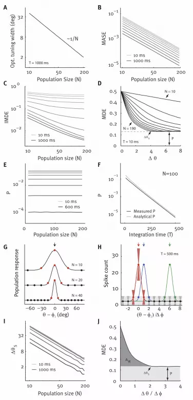
Figure 3 – Performance of Fisheroptimal codes
A. Optimal tuning width as a function of population size for T=1000 ms.
B. MASE of a neural population with independent noise and Fisher-optimal width as a function of
population size for ten different integration times T (ten values logarithmically spaced between 10 and
1000; light to dark grey). The width of the tuning functions is optimized for each N separately and chosen
such that it minimizes the MASE at this population size.
C. IMDE for the same Fisher-optimal populations as in B.
D. Family of neurometric functions for Fisher-optimal population codes at T=10 ms for N=10 to N=190
(right to left). is the point of saturation, P the pedestal error, also marked by the grey dashed line.
E. The pedestal error P is independent of the population size N (T like above, T=1000 ms is not shown for
clarity).
F. The pedestal error P depends on the integration time (black; independent of N) and analytical
approximation for P (grey).
G. For each population size, approximately three neurons are activated by each stimulus (red),
independent of the population size.
H. For coarse discrimination (red vs. green), the two stimuli activate disjoint sets of neurons determining
the pedestal error (red vs. green; error bars show 2 SD). For fine discrimination, the activated populations
overlap determining the initial region (red vs. blue).
I. Dependence of the point of saturation on the population size N (T like above).
J. Two parts of the neurometric function of Fisher-optimal population codes: the pedestal error P (light
grey) and the initial region (dark grey). Together they determine the IMDE. The neurometric function is
shown in units of difference in preferred orientation and is therefore independent of N. The pedestal error
is reached at (see Fig. S4). As , x-axis is rescaled and the area of the initial region
AIR goes to zero (see SI Text). Thus the IMDE converges to .
Figure 4 – Effect of noise correlations
A. Correlation matrices (Pearson correlation coefficient) of the four correlation structures studied
(N=100). Grey level indicates the level of correlation with dark values corresponding to high correlations.
Neurons have been arranged according to their preferred orientation, so correlations between cells with
similar tuning properties are close to the main diagonal. Diagonal entries have been removed for
visualization purposes.

B. MASE for a population of N=100 neurons as a function of integration time for the four different noise
correlation structures. MASE is shown relative to the independent population in logarithmic units. Colors
as shown in A.
C. MMSE of the same population for the same correlation structures.
D. IMDE of the same populations for the same correlation structures agrees with MMSE.
E. and F. MASE (dashed) and IMDE (solid) for a population of 100 neurons with stimulus-dependent
(red) or uniform correlations (blue) at 500 ms (E) and 10 ms (F) observation time as a function of average
correlation strength. Data is shown relative to the independent population in logarithmic units
G. and H. Neurometric functions for the four correlation structures at 500 ms (G) and at 10 ms (H)
integration time. The square marks , from which on stimulus-dependent correlations perform worse
than uniform correlations. In H. the crossing point lies effectively at . Data is also shown relative
to the independent population, smoothed and in logarithmic units on the y-axis in the insets.
Table 1 (1 column)
Acronym Definition
MDE Minimum discrimination error, eq. (3); ideal observer error in a discrimination task
IMDE Integrated minimum discrimination error, eq. (9); average MDE over all
MMSE Minimum mean squared error, eq. (10); ideal observer error in a reconstruction task
MASE Mean asymptotic squared error, eq. (4); approximation to the MMSE obtained by averaging over the inverse of Fisher information

A BStimulus
Neural response
Tuningfunctions
MD
E
DC
E
θ1 θ2
F
Firing rate

0 10 200
0.1
0.2
0.3
0.4
0.5
∆ θ
MD
E
D
IMDE optimal
Fisher optimalMMSE optimal
10−4
Tuning width (deg)
MA
SE
A 10 ms
1000 ms500 ms100 ms
2 10 50
10−2
10−1
IMD
E
Tuning width (deg)
2 10 50
CB
10−4
MM
SE
Tuning width (deg)
2 10 50
100
10−2
10−2
10 0
10 20010−5
10−3
10−1
Population size (N)
MA
SE
A
10−2
10−1
10 0
IMD
EB
10 0 2 4 6 80
0.1
0.2
0.3
0.4
0.5
∆ θ
MD
E
C
PT = 10 ms
0 100 200
10−4
10−2
P
E
2
8
32
10 200
Population size (N)
P
D
F
Analytical PMeasured P
10 ms1000 ms
50
50
20050
0 250 500
10−5
10−3
10−1
Integration time (T)
∆θ S
∆θS
Population size (N)
Population size (N)
N=100
I J
10 ms1000 ms
10 ms1000 ms
10 ms600 ms
N = 10
N = 190
0
0.1
0.2
0.3
0.4
0.5
MD
E
P
AIR
10 50 200
2
8
32
Population Size (N)
Opt
. tun
ing
wid
th (d
eg)
T = 1000 ms
0
10
20
30
Spik
e co
unt
−60 −30 0 30 60 (deg)
G H
N = 10
N = 20
N = 40
T = 500 ms
(θ − φ ) /0 2 4 6 8-2
∆θS
0 1 2 3 4
∆ θ / ∆ φ
∆ φiθ − φ i
Popu
lati
on re
spon
se
~1/N

101
102
103
−1
0
1
2
Integration time (T)
Rela
tive
MA
SE
C
101
102
103
−0.5
0
0.5
1
Integration time (T)
Rela
tive
IMD
E
B D
−1
0
1
2
3
Rela
tive
MM
SE
101
102
103
Integration time (T)
Uniform Stimulus Dep.
Limited Range Lim. Range x Stim. Dep.
0 0.05 0.15 0.3−2
−1.5
−1
−0.5
0
0.5
Rela
tive
Err
or
0 0.05 0.15 0.3
−1
−0.5
0
0.5
A
G HE F
500 ms 10 ms
IMDEMASE
∆
0.1
0.2
0.3
0.4
0.5
θ
MD
E
0 5 10 15
500 ms
400 20∆ θ
10 ms
0.1
0.2
0.3
0.4
0.5
Avg. correlation coefficient Avg. correlation coefficient
∆θc
∆θc

1
Optimal Population Coding, Revisited – Supporting Information
Philipp Berens1,2,3,4, Alexander S. Ecker1,2,3,4, Sebastian Gerwinn1,2,3, Andreas S. Tolias1,4,5,6, Matthias
Bethge1,2,3
1. Bernstein Centre for Computational Neuroscience Tübingen, Spemannstr. 41, 72076 Tübingen, Germany
2. Werner Reichardt Centre for Integrative Neuroscience and Institute of Theoretical Physics, University of Tübingen, 72076 Tübingen, Germany
3. Max Planck Institute for Biological Cybernetics, Computational Vision and Neuroscience Group, Spemannstr. 41, 72076 Tübingen, Germany
4. Baylor College of Medicine, Department of Neuroscience, One Baylor Plaza, Houston, TX 77030, USA
5. Michael E. DeBakey Veterans Affairs Medical Center, Houston, TX, USA
6. Department of Computational and Applied Mathematics, Rice University, Houston, TX 77005, USA

2
SI Methods 1: Details on the correlation matrix
Following Josic et al. (1), we model the stimulus-dependent covariance matrix as
.
Here, we set as the variance of cell i, i.e. we assume a Fano factor of 1. is
the correlation coefficient between cells i and j. We allow for both, stimulus and spatial influences on ,
by setting
The function models the influence of the stimulus-dependent component on the correlation
structure, while the function models the spatial component and is independent of . We use
with and , where controls
the length of the spatial decay and C the average correlation. The four possible correlation shapes arising
from this parameterization are illustrated in Fig. 4A. To obtain a desired mean level of correlations in a
population, we use the method described in Appendix E of Josic et al. (1).
SI Methods 2: Numerical computation of the MDE/IMDE
We approximate the integral of eq. (3) numerically via Monte-Carlo techniques (2, 3) by
where are M samples, drawn from the mixture distribution . The
factor corrects for the fact that by sampling from we weigh each sample pattern with its
probability. We used and evaluated for 500 equally spaced points between 0 deg
and 180 deg.
The IMDE and average neurometric functions were obtained by evaluating them at 20
different uniformly spaced between and , where is the difference between two preferred
orientations. This is sufficient since all codes considered here are shift symmetric with period
and because tuning curves are symmetric about the preferred orientation, only half a period needs to be

3
considered. We verified that 20 different reference directions were sufficient by repeating our simulations
for >40 reference directions.
SI Methods 3: Numerical estimation of the MMSE
The minimum mean squared error is achieved by the estimator which minimizes eq. (10). Based upon a
response generated from the stimulus-conditional distribution for stimulus , it is given by
where
is the posterior over stimuli given the response and is the distance
measured along the circle (4). The prior is uniform such that . We evaluate the above equations
for L discrete, regularly spaced and replace the integrals by sums. We obtain:
Simplifying we obtain
which is solved by using again L discrete, uniformly spaced as candidates. This discretization limits the
accuracy with which the MMSE can be estimated. This is a problem in particular for very good
estimators, for which L must be very large. Here, we chose L=500 and verified that the MMSE curves at
the highest SNR did not change when L was substantially increased. Using this equation we can compute
the MMSE as
Similar procedures have been used in (5, 6). In some scenarios, approximation procedures like those
presented in (6) can be helpful.

4
SI Text
In this section, we formally show (i) that a non-zero pedestal error exists in the large N limit, (ii) that the
saturation point for Fisher-optimal codes goes to zero as the population size N increases for fixed T
and (iii) derive a linear approximation to the pedestal error of Fisher-optimal codes. In particular, we use
this approximation to show that the pedestal error depends on the available decoding time alone.
Preliminary remarks
We first note that in Fisher-optimal codes the tuning width is inversely proportional to N (Fig. 3A), such
that
for some constant c. Only a few cells are active for any given stimulus and this number does not depend
on the population size N (Fig. 3G). The tuning curve spacing can be expressed in terms of the population
size as
.
Therefore, we can write w in terms of as
,
which holds for any N. Also, . We further note that the following relationship holds:
.
If the exponent k is sufficiently large, . Thus, the tuning function in our model can be
replaced by
,
which is of Gaussian form. This implies that we can rewrite the tuning functions as follows:
In this equation, i is the neuron index and the constants in w are absorbed into the function h. Note that
the tuning functions g and h are fixed templates for which only the domain changes with N (see Fig. 3G
and H). While is defined on , h is defined on , for even N. It follows that the

5
Fisher-optimal tuning functions drawn in units of (instead of ) are constant for different N (see Fig.
3G and H); the activity of a neuron only depends on , that is how many units of its preferred
orientation is away from the stimulus, independent of N.
Existence of the pedestal error
We first show that there is a lower bound on the minimum discrimination error between any pair of
stimuli, which is non-zero in the large N limit. To this end, we define an auxiliary population of neurons
with additive Gaussian noise with variance , the parameter that determines the baseline firing rate of
our tuning curves. The firing patterns of this population are distributed as:
,
where is the identity matrix of dimension N. The minimum discrimination error of this population
provides a lower bound on that of the populations with Poisson-like noise used in the main text, i.e.
Here, the subscripts p and q indicate that the MDE is calculated with respect to the pattern distribution p
and q, respectively. We can express the right hand side of this equation as
,
where . Equality holds since in the case of additive noise the linear discrimination
error is equal to the MDE (see SI Discussion). We now provide an upper bound for d’:
Here we use as defined above and the neuron index i ranges from to . We can now use
the upper bound on and use a Gaussian tuning function instead. Now
without loss of generality we assume and substitute , and from above. We obtain

6
where the i indicates the neuron index, not the complex number. Inserting into the above equation yields
To arrive at the last inequality note that
is the area under the density function of a Gaussian with standard deviation .We can approximate the
integral by the lower Riemann sum, i.e. by rectangles with height for positive i and
with height for negative i, respectively. Thus, we have
.
Substituting and including , we obtain the above inequality.
Thus d’ is bounded from above independent of N. Therefore,
(1)
independent of N and in particular also in the limit . This shows that there is a non-vanishing
pedestal error P for all N and for finite T.
Convergence of saturation point to zero
Next we show that the saturation point converges to zero for . We define as
.

7
We approximate the MDE of the whole population with N neurons by considering only two subsets of
neurons each that are most strongly activated by one of the two stimuli:
Here is chosen such that
.
Here, is the MDE achieved by the subpopulation with neurons in the set , for which holds
.
Because the tuning curves are identical in units of for different N, does not change with N and
therefore is also a constant in units of :
Finally, we define as
and note that and therefore as . Consequently, the area of the initial region
will shrink to zero, too, as
.
In particular, the neurometric functions for different N at fixed T are identical, when written as a function
of (Fig. S4). Although they show a different pedestal error for different T, they reach their pedestal
error at constant for all N and T considered (~2 ).
Approximation of the pedestal error P
Finally, we derive an analytically tractable approximation of the pedestal error. Looking only at two times
neurons in a Fisher-optimal model population, we can approximate the pedestal error with
arbitrary precision. We find for our model that such that only six cells suffice to achieve the same
error as the entire population. We adopt the following notation: is the activity by the maximally excited
neuron and and are the activities of the two neurons to the left and to the right. For the time being,
we omit the dependence on and assume we place the stimulus at the peak of neuron 0. This results in
the two average response vectors to the two stimuli and

8
and the respective stimulus conditional covariance matrices and . To
derive our linear approximation of the pedestal error, we calculate taking advantage
of the small subpopulation that needs to be considered, where . We obtain:
This yields:
The error of the optimal linear classifier (7) in this situation is
where is the cumulative distribution function. This equation provides a good approximation of the
pedestal error of the neurometric function of Fisher-optimal population codes (Fig. 3F). We can see the
dependence on time by rewriting the above expression:
where depends only on the tuning curves of the individual neurons. In
particular, are constant with growing N (as shown above), because we can rewrite the tuning function
as a function of . The above expression depends on the choice of the reference direction , so we
average again over and obtain
(2)
where the subscript indicates the dependence of on inherited from the tuning functions.
SI Discussion

9
Most other studies which investigated population codes in the discrimination framework measured the
minimal linear discrimination error, such as (8-11) as well as part 1 of (7). Few others such as (12) and
part 2 of (7) also consider non-linear approximations of the minimal discrimination error. However, none
of these studies computed the minimal discrimination error.
Linear approaches
The studies by Johnson (8), Snippe & Koenderink (9, 10) and Averbeck & Lee (7) used the
discriminability index d’ from signal detection theory:
Here, is the difference in average firing rate profiles across the population and
is the noise covariance matrix. The first two studies (8, 9) evaluated this equation for constant and in
the limit . Since is an approximation of the derivative of the population firing rate
profile for small
so that the two studies effectively study the linear part of the Gaussian Fisher Information. Similar
approaches have also been used by (9, 13, 14).
Averbeck & Lee (7) used d’ also for finite with . They then proceeded to
compute the minimum linear discrimination error
where is the standard normal cumulative distribution function. It might not be immediately obvious
why this computation really yields the minimal linear discrimination error. To see why this is the case,
observe that for two normal distributions with means and covariance matrices and equal
prior probabilities, Fisher’s Linear Discriminant is the optimal linear classifier (15). Its weight vector is
given by
where . The discriminability index d’ along w with

10
is
which is the same as the above expression. For one-dimensional data, the error can be computed from d’
with the formula used above (see also (7)).
While the LDE is equal to the MDE for additive Gaussian noise models, i.e. when with
, it does not capture the coding properties of a population code in the general case with
stimulus-dependent covariance matrices, e.g. for a Poisson-like Gaussian noise model, or for stimulus-
dependent correlations structures.
Non-linear approaches
As a second measure of coding quality, Averbeck & Lee (7) consider the Bhattacharyya distance ( ). It
is defined as
which is, in the general case, as difficult to compute as the MDE. For the Gaussian case it simplifies to
(1.4.3)
Previously, Kang et al. (12) had used the Chernoff distance ( ) as a measure of coding accuracy, which
is defined as
(1.4.4)
with . Interestingly, is a special case of obtained by setting . To compute the
Chernoff-distance, Kang et al. exploit the fact that they assume a Gaussian noise model and a population
with independent neurons and show that for this case, the optimal equals , so that they effectively use
instead of in their study.

11
In the Gaussian case, a simpler formula can be provided for computing (16):
The interest in and originates in the fact that both provide an upper bound on the MDE, the
Chernoff bound (17, 16):
(1.4.5)
The identical bound for is in general less tight than equation (1.4.5), as with equality if and
only if the optimal in equation (1.4.4). If both class-conditional distributions are Gaussians with
, the true optimum can be shown to lie at (16). For arbitrary population codes and
noise distributions, the question whether the Chernoff bound is tight is not straightforward to answer.
Kang et al. state that its tightness depends on the population size, the integration time and the shape of the
tuning curves (12). In summary, and provide useful upper bounds on the MDE but cannot be used
to measure the MDE directly.
SI Figures
Figure S1
Tuning curves with width optimized for various criteria (black). For better visualization of the population
structure, two additional tuning curves are shown in light grey.
A. and B. MASE-optimal tuning curve for 10 and 1000 ms, respectively.
C. and D. MMSE-optimal tuning curve for 10 and 1000 ms, respectively.
E. and F. IMDE-optimal tuning curve for 10 and 1000 ms, respectively.
Figure S2
Fig. 2 shows that the optimal tuning width with regard to the MASE is almost independent of time, but
varies slightly. The reason for this is that the two parts of Fisher Information, and , have
different time dependencies. For an independent population, we have

12
Thus is proportional to time and its optimum is fixed for varying T. is constant and does not
depend on time. Therefore, the relative importance of the two terms changes with time: While for small T
and are roughly on the same order of magnitude, dominates for large T.
When we plot the two extreme cases, and , corresponding to and ,
respectively, we find that they lead to slightly different optimal tuning widths. The graph shows
(solid) and (dashed).
Note that this behavior is only present for the Poisson-like Gaussian but not for the discrete Poisson noise
model. The Fisher Information of an independent Poisson distribution is
which is equal to the first term of Fisher Information in the Gaussian case, . For the Poisson noise
model, Fisher Information and therefore the MASE lead to a constant optimum completely independent
of time (see Fig. S3).
Figure S3
A-B. Replication of the results shown in Fig. 2 with Poisson noise (discrete spike counts). We set
As in Fig. 2, we compute the MASE (A) and the IMDE (B) as a function of the tuning width for short and
long time intervals (T=10, 100, 500, 1000 ms; light grey to black). The results are very similar to the
Gaussian case: Fisher Information leads to narrow tuning curve independent of time and the
discrimination error to broad tuning functions for short time intervals, and narrow ones for long time
intervals.
C-E. IMDE for a population of 100 independent neuron with Poisson-like noise and variable Fano factor
(Fano factor 0.25, 1, 4) as a function of tuning width at two different integration times (T=10 and 500 ms;
light grey and dark grey, respectively). We used samples for the numerical evaluation.
F-H. Same as in C-E but MASE of the same population.
Figure S4
Neurometric functions with rescaled x-axis of populations (N=10,…,190) with Fisher-optimal tuning
functions for different integration times (T=10 ms to 600 ms; light grey to dark grey) as a function of

13
. The rescaled neurometric functions for populations of different size and identical integration
time are identical. Note the log-scale on the y-axis. All neurometric functions level off at ,
independent of the population size.
Figure S5
Dependence of the critical , from which on populations with uniform correlations outperform
populations with stimulus-dependent correlations, on the available decoding time T. The value of
was extracted from the smoothed, relative versions of the neurometric functions.
Figure S6
Neurometric functions of two neural populations with independent noise and Fisher-optimal tuning
functions (Population 1: N=70, T=47ms; Population 2: N=50, T=130ms). The Fisher information of both
populations is almost equal (1000 vs. 1016) but the pedestal errors are quite different. Note that in this
case Fisher information and neurometric functions were calculated for a stimulus located at the peak of
one of the tuning functions and not averaged over stimuli.
SI References
1. Josić K, Shea-Brown E, Doiron B, de la Rocha J (2009) Stimulus-Dependent Correlations and Population Codes. Neural Computation 21:2774-2804.
2. Berens P, Gerwinn S, Ecker AS, Bethge M (2009) in Advances in Neural Information Processing
Systems 22: Proceedings of the 2009 Conference (MIT Press, Cambridge, MA), pp 90-98. 3. Hershey J, Olsen P (2007) in Acoustics, Speech and Signal Processing, 2007. ICASSP 2007. IEEE
International Conference on, pp IV-317-IV-320. 4. Berens P (2009) CircStat: a MATLAB toolbox for circular statistics. Journal of Statistical Software
31. 5. Bethge M, Rotermund D, Pawelzik K (2002) Optimal Short-Term Population Coding: When Fisher
Information Fails. Neural Computation 14:2317-2351. 6. Yaeli S, Meir R (2010) Error-based analysis of optimal tuning functions explains phenomena
observed in sensory neurons. Frontiers in Computational Neuroscience 4:130. 7. Averbeck BB, Lee D (2006) Effects of Noise Correlations on Information Encoding and Decoding. J
Neurophysiol 95:3633-3644. 8. Johnson KO (1980) Sensory discrimination: decision process. J. Neurophysiol 43:1771-1792.

14
9. Snippe H, Koenderink J (1992) Information in channel-coded systems: correlated receivers.
Biological Cybernetics 67:183-190. 10. Snippe HP, Koenderink JJ (1992) Discrimination thresholds for channel-coded systems. Biol.
Cybern. 66:543-551. 11. Pouget A, Thorpe SJ (1991) Connectionist models of orientation identification. Connection Science
3:127–142. 12. Kang K, Shapley RM, Sompolinsky H (2004) Information Tuning of Populations of Neurons in
Primary Visual Cortex. J. Neurosci. 24:3726-3735. 13. Seriès P, Stocker AA, Simoncelli EP (2009) Is the Homunculus “Aware” of Sensory Adaptation?
Neural Computation 21:3271-3304. 14. Mato G, Sompolinsky H (1996) Neural Network Models of Perceptual Learning of Angle
Discrimination. Neural Computation 8:270-299. 15. Duda RO, Hart PE, Stork DG (2000) Pattern Classification (Wiley & Sons). 2nd Ed. 16. Fukunaga K (1990) Introduction to statistical pattern recognition (Academic Pr). 17. Cover TM, Thomas JA (2006) Elements of Information Theory (Wiley-Interscience).

Orientation (deg)20 0 20
0
1
Rel.
Act
ivat
ion
(a. u
.)
Orientation (deg)20 0 20
0
1
Rel.
Act
ivat
ion
(a. u
.)
Orientation (deg)20 0 20
0
1Re
l. A
ctiv
atio
n (a
. u.)
10 m
s10
00
ms
Orientation (deg)20 0 20
0
1
Rel.
Act
ivat
ion
(a. u
.)
IMDE optimalMASE optimalA
B
C
DOrientation (deg)
20 0 20
0
1
Rel.
Act
ivat
ion
(a. u
.)
MMSE optimal
Orientation (deg)20 0 20
0
1Re
l. A
ctiv
atio
n (a
. u.)
E
F

2 10
10−4
Tuning width (deg)
MA
SE
meanJ 10 msmeanJ 100 msmeanJ 500 msmeanJ 1000 mscovJ

2 10 50
10−2
10−1
100
Tuning width (deg)
IMD
E
2 10 50
10−4
10−2
Tuning width (deg)
MA
SE
A B
Fano factor 0.25
T = 10 ms
T = 500 ms
10−4
10−2
MA
SE
10−4
10−2
MA
SE
10−4
10−2
MA
SE
10−2
10−1
100
IMD
E
10−2
10−1
100
IMD
E
10−2
10−1
100
IMD
E
2 10 50
Tuning width (deg)
2 10 50
Tuning width (deg)
2 10 50
Tuning width (deg)
2 10 50
Tuning width (deg)
2 10 50
Tuning width (deg)
2 10 50
Tuning width (deg)
C D E
F G H
T = 100 ms
T = 1000 ms
Fano factor 0.25
Fano factor 1
Fano factor 1
Fano factor 4
Fano factor 4

0 1 2 3 4
10−1
∆ θ / ∆ φ
MD
E
10 ms600 ms
10−3
10−5

0
5
10
15
T
∆ θ
10 100 1000
c

N=50, 130ms, J=1016
0 5 100
0.1
0.2
0.3
0.4
0.5
∆ θ
MD
E
N=70, 47ms, J=1000