Embed Size (px)
Citation preview
Orbital Lifetime Predictions of Low EarthOrbit Satellites and the eect of a DeOrbitSail
by
Michael A. Aul
Thesis presented in partial fullment of the requirements for the degree of
Master of Engineering at Stellenbosch University
Department of Electrical and Electronic Engineering
University of Stellenbosch
Private Bag X1, 7602, Matieland, South Africa.
Supervisors: Prof. W. H. Steyn
Dr. B. D. L. Opperman
December 2013
i
Declaration
By submitting this thesis electronically, I declare that the entirety of the work contained
therein is my own, original work, that I am the owner of the copyright thereof (unless to
the extent explicitly otherwise stated), that reproduction and publication thereof by Stel-
lenbosch University will not infringe any third party rights and that I have not previously
in its entirety or in part submitted it for obtaining any qualication.
Signature: . . . . . . . . . . . . . . . . . . . . . . .
M. A. Aul
December 2013
Date: . . . . . . . . . . . . . . . . . . . . . . . . . .
Copyright © 2013 Stellenbosch University.
All rights reserved.
Stellenbosch University http://scholar.sun.ac.za
ii
Abstract
Throughout its lifetime in space, a spacecraft is exposed to risk of collision with orbital
debris or operational satellites. This risk is especially high within the Low Earth Orbit
(LEO) region where the highest density of space debris is accumulated.
This study investigates orbital decay of some LEO micro-satellites and accelerating orbit
decay by using a deorbitsail. The Semi-Analytical Liu Theory (SALT) and the Satellite
Toolkit was employed to determine the mean elements and expressions for the time rates
of change. Test cases of observed decayed satellites (Iridium-85 and Starshine-1) are used
to evaluate the predicted theory. Results for the test cases indicated that the theory tted
observational data well within acceptable limits.
Orbit decay progress of the SUNSAT micro-satellite was analysed using relevant orbital
parameters derived from historic Two Line Element (TLE) sets and comparing with decay
and lifetime prediction models. The study also explored the deorbit date and time for a
1U CubeSat (ZACUBE-01).
A proposed orbital debris solution or technology known as deorbitsail was also investigated
to gain insight in sail technology to reduce the orbit life of spacecraft with regards to de-
orbiting using aerodynamic drag. The deorbitsail technique signicantly increases the
eective cross-sectional area of a satellite, subsequently increasing atmospheric drag and
accelerating orbit decay. The concept proposed in this work introduces a very useful
technique of orbit decay as well as deorbiting of spacecraft.
Stellenbosch University http://scholar.sun.ac.za
iii
Samevatting
Gedurende sy leeftyd in die ruimte word 'n ruimtetuig blootgestel aan die risiko van 'n
botsing met ruimterommel of met funksionele satelliete. Hierdie risiko is veral hoog in die
lae-aardbaan gebied waar die hoogste digtheid ruimterommel voorkom.
Hierdie studie ondersoek die wentelbaanverval van sommige Lae-aardbaan mikrosatelliete
asook die versnelde baanverval wanneer van 'n deorbitaal meganisme gebruik gemaak word.
Die Semi-Analitiese Liu Teorie en die Satellite Toolkit sagtewarepakket is gebruik om die
gemiddelde baan-elemente en uitdrukkings vir hul tyd-afhanlike tempo van verandering
te bepaal. Toetsgevalle van waargenome vervalde satelliete (Iridium-85 en Starshine-1) is
gebruik om die verloop van die voorspelde teoretiese verval te evalueer. Resultate vir die
toetsgevalle toon dat die teorie binne aanvaarbare perke met die waarnemings ooreenstem.
Die verloop van die SUNSATmikrosatelliet se wentelbaanverval is ook ontleed deur gebruik
te maak van historiese Tweelyn Elemente datastelle en dit te vergelyk met voorspelde baan-
elemente. Die studie het ook ondersoek ingestel na die voorspelde baan-verbyval van 'n
1-eenheid cubesat (ZACUBE-01).
Die impak op wentelbaanverval deur 'n voorgestelde oplossing vir die beperking van
ruimterommel, 'n deorbitaalseil, is ook ondersoek. So seil verkort 'n satelliet se ruimte-
leeftyd deur sy eektiewe deursnee-area te vergroot en dan van verhoogde atmosferiese
sleur en sonstralingsdruk gebruik te maak om die vervalproses te versnel. Hierdie voorgestelde
konsep is 'n moontlike nuttige tegniek vir versnelde baanverval en beheerde deorbitalering
van ruimtetuie om ruimterommel te verminder.
Stellenbosch University http://scholar.sun.ac.za
iv
Acknowledgements
First and foremost I would like to thank God for the continuous guidance and mercy
throughout my stay in South Africa. I forever remain grateful. My profound gratitude goes
to my supervisors Prof. Willem H. Steyn and Dr. Ben D. L. Opperman for their guidance,
valuable ideas and contributions towards the completion of my project. The continuous
support in many aspects provided by Prof. Willem H. Steyn is greatly appreciated.
I would like to acknowledge the South African National Astrophysics and Space Science
Programme (NASSP), University of Cape Town for awarding me the bursary to pursue
further studies. Many thanks to the NASSP administrator, Mrs Nicky Walker, for her
kind gesture and assistance. I sincerely appreciate the support and cooperation of my
NASSP classmates and friends, Samuel Oronsaye, Temwani Phiri and Doreen Agaba.
I am grateful to the South African National Space Agency (SANSA) Space Science team for
creating the enabling environment for my research. The warm hospitality, encouragement,
and support granted me is highly acknowledged. I appreciate the support of Nicholas
Ssessanga and Vumile Tyalimpi for their unwavering assistance. Many thanks to Mrs
Elda Saunderson for proofreading my work.
I would like to express my heartfelt thanks to my parents Mr and Mrs Aul for all around
continuous support from elementary school to present. Best of thanks to my brothers for
their prayers and support. I am highly indebted to you all. Special thanks to my very best
friend Ms. Lydia Quaye for her love, prayers and patience. May the good Lord reward
you all.
Stellenbosch University http://scholar.sun.ac.za
Contents
Declaration i
Abstract ii
SameVatting iii
Acknowledgement iv
Content iv
List of Figures iv
List of Tables iv
Nomenclature iv
1 Introduction 1
1.1 Study Objectives . . . . . . . . . . . . . . . . . . . . . . . . . . . . . . . . 1
1.2 Thesis Overview . . . . . . . . . . . . . . . . . . . . . . . . . . . . . . . . . 2
1.3 Research Motivation . . . . . . . . . . . . . . . . . . . . . . . . . . . . . . 2
2 Literature Review and Problem Description 4
2.1 Introduction . . . . . . . . . . . . . . . . . . . . . . . . . . . . . . . . . . . 4
2.2 Historical Perspective . . . . . . . . . . . . . . . . . . . . . . . . . . . . . . 4
v
Stellenbosch University http://scholar.sun.ac.za
CONTENTS vi
2.2.1 Reordering the Universe . . . . . . . . . . . . . . . . . . . . . . . . 5
2.2.2 Onset of the New Era . . . . . . . . . . . . . . . . . . . . . . . . . 6
2.3 Space Debris Problem . . . . . . . . . . . . . . . . . . . . . . . . . . . . . 7
2.3.1 Concerns and Threats posed by Space Debris . . . . . . . . . . . . 9
2.3.2 Mitigation Guidelines . . . . . . . . . . . . . . . . . . . . . . . . . . 10
2.4 DeOrbitSail Concept . . . . . . . . . . . . . . . . . . . . . . . . . . . . . . 11
2.5 Summary . . . . . . . . . . . . . . . . . . . . . . . . . . . . . . . . . . . . 13
3 Theoretical Background 14
3.1 Introduction . . . . . . . . . . . . . . . . . . . . . . . . . . . . . . . . . . . 14
3.2 Equations of Motion . . . . . . . . . . . . . . . . . . . . . . . . . . . . . . 14
3.2.1 Two-Body Equation . . . . . . . . . . . . . . . . . . . . . . . . . . 16
3.2.1.1 Assumptions . . . . . . . . . . . . . . . . . . . . . . . . . 16
3.2.1.2 Equation of Relative Motion . . . . . . . . . . . . . . . . . 16
3.2.2 Constants of Motion . . . . . . . . . . . . . . . . . . . . . . . . . . 19
3.2.2.1 Energy Law . . . . . . . . . . . . . . . . . . . . . . . . . . 19
3.2.2.2 Angular Momentum . . . . . . . . . . . . . . . . . . . . . 20
3.2.2.3 Trajectory Equation . . . . . . . . . . . . . . . . . . . . . 20
3.3 Satellite State . . . . . . . . . . . . . . . . . . . . . . . . . . . . . . . . . . 21
3.3.1 Classical Orbit Parameters . . . . . . . . . . . . . . . . . . . . . . . 21
3.4 Coordinate Systems and Transformations . . . . . . . . . . . . . . . . . . . 23
3.4.1 Reference Systems . . . . . . . . . . . . . . . . . . . . . . . . . . . 24
3.4.1.1 Earth Centred Inertial (ECI) System . . . . . . . . . . . . 24
3.4.1.2 Earth Centred Earth Fixed (ECEF) System . . . . . . . . 24
3.4.1.3 Geographic Co-ordinates . . . . . . . . . . . . . . . . . . . 25
3.4.1.4 Perifocal Coordinate System . . . . . . . . . . . . . . . . . 25
Stellenbosch University http://scholar.sun.ac.za
CONTENTS vii
3.4.2 Coordinate Transformations . . . . . . . . . . . . . . . . . . . . . . 26
3.4.2.1 Transformation from ECEF to ECI . . . . . . . . . . . . . 26
3.4.2.2 Transformation between Perifocal Coordinates and ECI . . 27
3.4.2.3 Position and Velocity from Orbital Elements . . . . . . . . 28
3.5 Two-Line Element Sets . . . . . . . . . . . . . . . . . . . . . . . . . . . . . 29
3.6 Summary . . . . . . . . . . . . . . . . . . . . . . . . . . . . . . . . . . . . 30
4 Orbit Perturbations and Decay Employed in SALT 31
4.1 Introduction . . . . . . . . . . . . . . . . . . . . . . . . . . . . . . . . . . . 31
4.2 Perturbation Eects on Orbital Elements . . . . . . . . . . . . . . . . . . . 32
4.3 Osculating and Mean Elements . . . . . . . . . . . . . . . . . . . . . . . . 33
4.4 Variational Equations of Motion implemented in SALT . . . . . . . . . . . 34
4.5 Eects of Earth Oblateness and Gravity . . . . . . . . . . . . . . . . . . . 35
4.5.1 Non-spherical Gravity Potential . . . . . . . . . . . . . . . . . . . . 35
4.5.2 Earth Oblateness . . . . . . . . . . . . . . . . . . . . . . . . . . . . 36
4.6 Atmospheric Drag Eects . . . . . . . . . . . . . . . . . . . . . . . . . . . 39
4.6.1 Evaluating Atmospheric Density . . . . . . . . . . . . . . . . . . . . 41
4.6.2 Atmospheric Density Model . . . . . . . . . . . . . . . . . . . . . . 42
4.7 Implementation of SALT in LIFTIM . . . . . . . . . . . . . . . . . . . . . 43
4.7.1 Program Structure and Functionality . . . . . . . . . . . . . . . . . 43
4.7.1.1 Elliptical Option . . . . . . . . . . . . . . . . . . . . . . . 44
4.7.1.2 Circular Option . . . . . . . . . . . . . . . . . . . . . . . . 45
4.8 Summary . . . . . . . . . . . . . . . . . . . . . . . . . . . . . . . . . . . . 46
5 Simulation Environment 47
5.1 Introduction . . . . . . . . . . . . . . . . . . . . . . . . . . . . . . . . . . . 47
5.2 LIFTIM Application . . . . . . . . . . . . . . . . . . . . . . . . . . . . . . 47
Stellenbosch University http://scholar.sun.ac.za
CONTENTS viii
5.3 Data Preparation . . . . . . . . . . . . . . . . . . . . . . . . . . . . . . . . 47
5.3.1 Drag Coecients . . . . . . . . . . . . . . . . . . . . . . . . . . . . 49
5.3.2 Decay Predictions . . . . . . . . . . . . . . . . . . . . . . . . . . . . 53
5.3.2.1 STK Lifetime Tool . . . . . . . . . . . . . . . . . . . . . . 54
5.4 Eects of using a DeOrbitSail . . . . . . . . . . . . . . . . . . . . . . . . . 56
5.5 Summary . . . . . . . . . . . . . . . . . . . . . . . . . . . . . . . . . . . . 57
6 Results and Discussion 58
6.1 Introduction . . . . . . . . . . . . . . . . . . . . . . . . . . . . . . . . . . . 58
6.2 Schatten data adopted in LIFTIM . . . . . . . . . . . . . . . . . . . . . . . 58
6.3 Comparative Decay Results without a DeOrbitSail Mechanism . . . . . . . 59
6.3.1 Iridium-85 Satellite . . . . . . . . . . . . . . . . . . . . . . . . . . . 59
6.3.2 Starshine-1 Satellite . . . . . . . . . . . . . . . . . . . . . . . . . . 63
6.3.3 SUNSAT . . . . . . . . . . . . . . . . . . . . . . . . . . . . . . . . 66
6.3.4 1U CubeSAT (ZACUBE-01) . . . . . . . . . . . . . . . . . . . . . . 71
6.4 Theoretical Decay Results using a DeOrbitSail Mechanism . . . . . . . . . 75
6.4.1 Iridium-85 Satellite . . . . . . . . . . . . . . . . . . . . . . . . . . . 76
6.4.2 Starshine-1 Satellite . . . . . . . . . . . . . . . . . . . . . . . . . . 76
6.4.3 SUNSAT . . . . . . . . . . . . . . . . . . . . . . . . . . . . . . . . . 77
6.4.4 1U CubeSAT (ZACUBE-01) . . . . . . . . . . . . . . . . . . . . . . 77
6.5 Discussion . . . . . . . . . . . . . . . . . . . . . . . . . . . . . . . . . . . 78
6.5.1 Decay Predictions . . . . . . . . . . . . . . . . . . . . . . . . . . . . 78
6.5.2 Eects of the DeOrbitSail Mechanism . . . . . . . . . . . . . . . . . 80
6.6 Summary . . . . . . . . . . . . . . . . . . . . . . . . . . . . . . . . . . . . 81
7 Conclusion and Future Work 83
7.1 Summary of Study . . . . . . . . . . . . . . . . . . . . . . . . . . . . . . . 84
Stellenbosch University http://scholar.sun.ac.za
CONTENTS ix
7.1.1 Lifetime Predictions . . . . . . . . . . . . . . . . . . . . . . . . . . 84
7.1.2 DeOrbitSail Mechanism . . . . . . . . . . . . . . . . . . . . . . . . 86
7.2 Conclusion . . . . . . . . . . . . . . . . . . . . . . . . . . . . . . . . . . . . 86
7.3 Further Research and Recommendation . . . . . . . . . . . . . . . . . . . . 87
Bibliography 87
Appendix 87
A Derivation of Equations of Motion 93
A.1 Two-Body Problem . . . . . . . . . . . . . . . . . . . . . . . . . . . . . . . 93
A.2 Specic Mechanical Energy is a Constant . . . . . . . . . . . . . . . . . . . 94
A.3 Specic Angular Momentum is a Constant . . . . . . . . . . . . . . . . . . 95
B Description of Files 97
B.1 Two-Line Element (TLE) le . . . . . . . . . . . . . . . . . . . . . . . . . . 97
B.2 Subroutine and Microow . . . . . . . . . . . . . . . . . . . . . . . . . . . 98
B.3 Input File Format used in Decay Analysis [1] . . . . . . . . . . . . . . . . . 102
B.3.1 Iridium-85 Input File for Decay Prediction . . . . . . . . . . . . . . 103
B.3.2 Starshine-1 Input File for Decay Prediction . . . . . . . . . . . . . . 104
B.3.3 SUNSAT Input File for Decay Prediction . . . . . . . . . . . . . . . 105
B.3.4 ZACUBE-01 Input File for Decay Prediction . . . . . . . . . . . . . 106
C M-FILES 107
C.1 Routine for Estimated Drag Sail Size . . . . . . . . . . . . . . . . . . . . . 107
C.2 TLE History File . . . . . . . . . . . . . . . . . . . . . . . . . . . . . . . . 108
C.3 Routine for Computing the various Decay Dates . . . . . . . . . . . . . . 111
C.4 Routine for Data in STK . . . . . . . . . . . . . . . . . . . . . . . . . . . . 113
Stellenbosch University http://scholar.sun.ac.za
CONTENTS x
D Predicted Decay Dates using STK 115
D.1 Iridium-85 Satellite . . . . . . . . . . . . . . . . . . . . . . . . . . . . . . . 115
D.2 Starshine-1 Satellite . . . . . . . . . . . . . . . . . . . . . . . . . . . . . . . 116
D.3 ZACUBE-01 Satellite . . . . . . . . . . . . . . . . . . . . . . . . . . . . . . 116
E De-orbitsail Technique 117
E.1 Conguration of a sail membrane . . . . . . . . . . . . . . . . . . . . . . . 117
E.2 Observed Monthly Mean Solar Flux Data . . . . . . . . . . . . . . . . . . . 118
Stellenbosch University http://scholar.sun.ac.za
List of Figures
2.1 Computer generated image of orbital debris in LEO [17]. . . . . . . . . . . 7
2.2 LEO Environment Projection (LEGEND Study) [15]. . . . . . . . . . . . . 8
2.3 Monthly number of catalogued objects in Earth orbit by object type [20]. . 9
2.4 Typical deployed 1.7× 1.7m sail [28]. . . . . . . . . . . . . . . . . . . . . . 12
3.1 Illustration of Kepler's First Law. . . . . . . . . . . . . . . . . . . . . . . . 15
3.2 Illustration of Kepler's Second Law. . . . . . . . . . . . . . . . . . . . . . . 15
3.3 Two-body System adapted from [3]. . . . . . . . . . . . . . . . . . . . . . . 17
3.4 Position vector of satellite in orbit [30]. . . . . . . . . . . . . . . . . . . . . 18
3.5 Classical orbit elements [55]. . . . . . . . . . . . . . . . . . . . . . . . . . . 22
3.6 (a) Earth Centred Inertial (ECI) Reference Frame. (b) ECEF and ECI
frames related by changing sidereal time θ. . . . . . . . . . . . . . . . . . 24
3.7 (a) Geographic coordinates [12]. (b) Illustration of Geodetic and Geocentric
latitudes. . . . . . . . . . . . . . . . . . . . . . . . . . . . . . . . . . . . . 25
3.8 A perifocal coordinate system adapted from [34]. . . . . . . . . . . . . . . . 26
3.9 Transformation from perifocal to ECI co-ordinate system using the three
Euler angles ω, i,Ω [31]. . . . . . . . . . . . . . . . . . . . . . . . . . . . . 28
4.1 General representation of secular and periodic variations of an orbital ele-
ment [30]. . . . . . . . . . . . . . . . . . . . . . . . . . . . . . . . . . . . . 33
4.2 Height vs. density for F10.7 values using the MSISE-90 model. . . . . . . . 42
xi
Stellenbosch University http://scholar.sun.ac.za
LIST OF FIGURES xii
4.3 Actual (historic) and predicted smoothed monthly mean solar ux values
at three activity levels required for predicting the atmospheric density. . . 42
4.4 Actual (historic) and predicted smoothed monthly mean magnetic index
values at three activity levels required for predicting the atmospheric density. 43
5.1 SUNSAT position errors using various drag coecients adapted from [12]. . 51
5.2 Iridium-85 position errors using various drag coecients adapted from [12]. 51
5.3 Starshine-1 position errors using various drag coecients adapted from [12]. 52
5.4 Dependence of orbital lifetime on drag coecient for Starshine-1 satellite. . 52
5.5 STK Lifetime Tool (GUI for SUNSAT). . . . . . . . . . . . . . . . . . . . . 55
5.6 Comparison between Solar Flux Data for LIFTIM and Schatten. . . . . . . 56
6.1 Comparison in semi-major axis of Iridium-85. . . . . . . . . . . . . . . . . 59
6.2 Comparison in (a) eccentricity (b) inclination for Iridium-85. . . . . . . . . 60
6.3 (a) Comparison in apogee height. (b) Predicted decay date of Iridium-85
using LIFTIM and (c) STK. . . . . . . . . . . . . . . . . . . . . . . . . . . 61
6.4 Predicted orbit decay of Iridium-85 with and without Schatten solar ux
data. . . . . . . . . . . . . . . . . . . . . . . . . . . . . . . . . . . . . . . . 62
6.5 Comparison in (a) semi-major axis. (b) eccentricity of Starshine-1. . . . . . 63
6.6 Comparison in (a) inclination. (b) apogee height of Starshine-1. . . . . . . 64
6.7 Predicted decay date of Starshine-1 using (a) LIFTIM. (b) STK . . . . . . 65
6.8 Predicted orbit decay of Starshine-1 with and without Schatten solar ux
data. . . . . . . . . . . . . . . . . . . . . . . . . . . . . . . . . . . . . . . . 66
6.9 (a) Average orbital height of SUNSAT since launch. (b) Evolution of semi-
major axis from epoch until 1st Nov. 2012. . . . . . . . . . . . . . . . . . . 67
6.10 Evolution of (a) eccentricity. (b) inclination of SUNSAT from epoch until
1st Nov. 2012 . . . . . . . . . . . . . . . . . . . . . . . . . . . . . . . . . . 68
6.11 (a) Comparison in apogee height from epoch until 1st Nov. 2012. (b)
Predicted decay date of SUNSAT at two solar activity levels using LIFTIM. 69
Stellenbosch University http://scholar.sun.ac.za
LIST OF FIGURES xiii
6.12 Predicted decay date of SUNSAT using (a) STK. (b) LIFTIM with and
without Schatten solar ux data.. . . . . . . . . . . . . . . . . . . . . . . . 70
6.13 Spectrum distribution of eccentricity for SUNSAT. . . . . . . . . . . . . . 71
6.14 Evolution of (a) semi-major axis. (b) eccentricity of ZACUBE-01. . . . . . 72
6.15 Evolution of (a) inclination. (b) apogee height of ZACUBE-01. . . . . . . . 73
6.16 Predicted decay date of ZACUBE-01 (a) at two solar activity levels using
LIFTIM. (b) STK. . . . . . . . . . . . . . . . . . . . . . . . . . . . . . . . 74
6.17 Predicted orbit decay of ZACUBE-01 with and without Schatten data. . . 75
6.18 Estimates of sail size to deorbit in 25 years. . . . . . . . . . . . . . . . . . 75
6.19 Predicted lifetime comparison of Iridium-85 with and without a 10m2 sail. 76
6.20 Predicted lifetime comparison of Starshine-1 with and without a 10 m2 sail. 76
6.21 Predicted lifetime comparison of SUNSAT with and without a 10 m2 sail. . 77
6.22 Predicted lifetime comparison of ZACUBE-01 with and without a 10 m2
sail using LIFTIM. . . . . . . . . . . . . . . . . . . . . . . . . . . . . . . . 77
7.1 Orbit lifetime estimation process [7]. . . . . . . . . . . . . . . . . . . . . . 85
B.1 LIFTIM ow chart showing the routines for circular and elliptical cases [1]. 101
D.1 Predicted decay date with a 10 m2 sail using STK for Iridium-85 satellite. 115
D.2 Predicted decay date with a 10 m2 sail using STK for Starshine-1 satellite. 116
D.3 Predicted decay date with a 10 m2 sail using STK for ZACUBE-01 satellite. 116
E.1 Sail concept, stowed (left) and deployed (right) [28]. . . . . . . . . . . . . . 117
E.2 Observed monthly mean solar ux data . . . . . . . . . . . . . . . . . . . . 118
Stellenbosch University http://scholar.sun.ac.za
List of Tables
3.1 Relationship between conic section and eccentricity. . . . . . . . . . . . . . 20
3.2 Parameters dening an ellipse [4]. . . . . . . . . . . . . . . . . . . . . . . . 22
3.3 Transforming position and velocity vectors to Kepler elements [4]. . . . . . 23
4.1 Pertubing eects on orbital elements. . . . . . . . . . . . . . . . . . . . . . 33
5.1 Geometry of decayed satellites used in evaluating SALT. . . . . . . . . . . 48
5.2 Two-Line Elements at time closest after launch. . . . . . . . . . . . . . . . 48
5.3 TLE-derived state vectors and osculating orbital elements of dates closest
to launch. . . . . . . . . . . . . . . . . . . . . . . . . . . . . . . . . . . . . 49
5.4 Drag coecients, position and velocity errors for SUNSAT, Iridium-85 and
Starshine-1. . . . . . . . . . . . . . . . . . . . . . . . . . . . . . . . . . . . 50
5.5 Optimum drag coecients . . . . . . . . . . . . . . . . . . . . . . . . . . . 53
5.6 Orbital parameters for ZACUBE-01. . . . . . . . . . . . . . . . . . . . . . 54
6.1 Predicted deorbit dates for test case satellites. . . . . . . . . . . . . . . . . 79
6.2 Predicted deorbit dates & time for SUNSAT and ZACUBE-01. . . . . . . . 80
6.3 LIFTIM predicted orbital lifetime with and without a deorbitsail. . . . . . 81
6.4 STK predicted orbital lifetime with and without a deorbitsail. . . . . . . . 82
B.1 Functional grouping of Subprograms . . . . . . . . . . . . . . . . . . . . . 98
xiv
Stellenbosch University http://scholar.sun.ac.za
Nomenclature
Abbreviations and Acronyms
1U 1-Unit
ADR Active Debris Removal
ASCII American Standard Code for Information Interchange
BC Ballistic Coecient
CIRA COSPAR International Reference Atmosphere
CPUT Cape Peninsula Univeristy of Technology
DCM Direction Cosine Matrix
DTM Drag Temperature Model
ECI Earth Centred Inertial
ECEF Earth Centred Earth Fixed
FCC Federal Communications Commission
FFT Fast Fourier Transform
F'SATI French South African Institute of Technology
GCI Geocentric Inertial
GEO Geosynchronous Orbit
GMST Greenwich Meridian Standard Time
GSFC Goddard Space Flight Center
GUI Graphical User Interface
HPOP High Precision Orbit Propagator
IADC Inter-Agency Space Debris Coordination Committee
IKAROS Interplanetary Kite-Craft Accelerated by Radiation of the SUN
ISS International Space Station
LEGEND LEO-to-GEO Environmental Debris Model
LEO Low Earth Orbit
Stellenbosch University http://scholar.sun.ac.za
LIFTIM Lifetime Prediction Program
MEO Medium Earth Orbit
MSAFE MSFC Solar Activity Future Estimation Model
MSFC Marshall Space Flight Center
MSIS Mass Spectrometer Incoherent Scatter
NASA National Aeronautics and Space Administration
NOAA National Oceanic and Atmospheric Administration
NORAD North American Aerospace Defense Command
SALT Semi Analytical Liu Theory
SGP4 Simplied General Perturbation No. 4
SLR Satellite Laser Ranger
STK Satellite ToolKit
TLE Two Line Element
USSSN United States Space Surveillance Network
Greek Symbols
µ Gravitational Parameter
ν True Anomaly
ε Specic Mechanical Energy
Ω Right Ascension of the Ascending Node
Υ Vernal Equinox
ω Argument of Perigee
αr Right Ascension
δd Declination
λ Longitude (Chapter 3)
φ Latitude (Chapter 3)
Stellenbosch University http://scholar.sun.ac.za
Φ Potential Function
ϕ Geocentric Latitude (Chapter 4)
ρ Atmospheric Density
θ Geographic Longitude (Chapter 4)
Lowercase Letters
m Mass
a Semi-major Axis
e Eccentricity
mi Mass of ithBody
mi Time rate of change of mass of the ith body
h Specic Angular Momentum
p Semi-parameter
i Inclination
ra Apogee Radius
rp Perigee Radius
b Semi-minor Axis
n Mean Motion
n Nodal Vector
ω⊕ Earth Rotation Rate (Chapter 3)
θnm Equilibrium longitude for Jnm
cD Drag Coecient
∇ Gradient operator (del)
adrag Acceleration due to Atmospheric Drag
r Geocenric distance (Chapter 4)
ωa Earth rotational speed (Chapter 4)
(ra)d Average rate of change in ra due to drag
Stellenbosch University http://scholar.sun.ac.za
(rp)d Average rate of change in rp due to drag
am Rate of change of the transformed mean equation of motion of a
em Rate of change of the transformed mean equation of motion of e
im Rate of change of the transformed mean equation of motion of i
ωm Rate of change of the transformed mean equation of motion of ω
Ωm Rate of change of the transformed mean equation of motion of Ω
Mm Rate of change of the transformed mean equation of motion of M
Uppercase Letters
M Mass of Earth
G Gravitational Constant
R Radius (Chapter 3)
R Position Vector
Ri Acceleration vector of the ith body
Ri Velocity vector of the ithbody
FDrag Drag Force
FThrust Thrust Force
FSUN External Force from the SUN
FMOON External Force from the MOON
V Satellite's Velocity
V Velocity Vector
N Ascending Node
M Mean Anomaly
E Eccentric Anomaly
R Acceleration (Chapter 4)
Xω, Yω, Zω Co-ordinate Axes
P,Q Unit Vectors
Stellenbosch University http://scholar.sun.ac.za
B∗ Drag Term
J2, J3, J4 Harmonic Terms
A Cross-sectional Area
Re Equatorial radius of the Earth (Chapter 4)
Pn Legendre polynomials of degree n, order 0
Pnm Associated Legendre polynomials of degree n, order m
Ap Magnetic Index
F10.7 Solar Flux
H Altitude (Chapter 4)
Stellenbosch University http://scholar.sun.ac.za
Chapter 1
Introduction
1.1 Study Objectives
The aim of this project is to study and investigate the present orbit decay progress of a
Low Earth Orbit satellite (SUNSAT) by using relevant orbital parameters derived from
historic NORAD Two Line Element (TLE)1 [13] sets and comparing it with decay and
lifetime prediction models such as the Semi-Analytical Liu Theory (SALT) [1] and Satellite
Toolkit (STK) [44].
The study objectives are:
1. Investigate the accuracy of predicted orbital element evolution over (test) satellite's
lifetime (re-entry date).
2. Investigate the eects of orbit perturbations on time evolution of satellite orbital
elements and the orbital lifetime of SUNSAT.
3. Test the theory and long-term predicted solar and magnetic data sets by implement-
ing relevant algorithms and software packages and comparing the theoretical results
with observed/ historic TLE-derived orbital parameters.
4. Investigate the FP7 DeOrbitSail mission [42] to reduce the lifetime of satellites with
regards to deorbiting using aerodynamic drag.
1TLE - data format used to convey sets of orbital elements that describe the orbits of Earth-orbitingsatellites. The format is specied by the North American Aerospace Defence Command (NORAD) andthe National Aeronautics and Space Administration (NASA).
1
Stellenbosch University http://scholar.sun.ac.za
CHAPTER 1. INTRODUCTION 2
1.2 Thesis Overview
In Chapter 2, background information on historical concepts, an introduction to the space
debris problem as well as the DeOrbitSail mission is presented. Chapter 3 focuses on the-
oretical overview on orbit fundamentals. The equations developed serve as an illustration
for understanding two-body mechanics. Co-ordinate frames used to describe the orienta-
tion and position of a satellite are introduced. Co-ordinate transformation matrices needed
for vector transformation between the various co-ordinate frames are also explained.
Chapter 4 deals with orbit perturbations and decay as implemented in SALT. The mathe-
matical modelling of the orbit perturbation forces and methods used in a general perturbed
orbit are explained. The eects of perturbations on a satellite's orbital parameters are
presented. The software structure is discussed. The SALT employed in this study is
presented as well as the atmospheric model, and its associated dynamics are discussed.
The theme of Chapter 5 is the simulation environment. Description of the methods used in
obtaining the results are presented. The results of this study are presented and discussed in
Chapter 6. A conclusion, with a summary of the project ndings, some recommendations
and future work are given in Chapter 7.
1.3 Research Motivation
Spacecraft are exposed to the risk of collisions with orbital debris2 and operational satel-
lites throughout its launch, early orbit and mission phases. This risk is especially high
during passage through, or operations within, the Low Earth Orbit (LEO) region, because
this region is highly concentrated with space junk. Understanding the lifetime of these
spacecraft in LEO would be useful for studying the long term evolution of space objects
in assessing the risk of potential collision of these objects with active spacecraft.
An increasing number of countries have active or planned space programmes which would
result in the growth of the number of satellites to be launched over the next decade.
Satellite launches both replace satellites whose operational lifes have ended and place new
satellites in orbit. The outcome of these current and future satellite launch activities is
and will be an increase in the number of satellites and launch vehicle upper stages in
orbit. There are also several satellites launched into LEO for short duration missions.
2Orbital debris, also known as space debris, space junk or space waste, is a collection of objects inorbit around Earth that were created by humans but no longer serve any useful purpose. These objectsconsist of everything from spent rocket stages and defunct satellites to erosion, explosion and collisionfragments.
Stellenbosch University http://scholar.sun.ac.za
CHAPTER 1. INTRODUCTION 3
The growing population of spacecraft that have completed their missions, especially those
launched for short-duration, low altitude missions, continues to accumulate, which will
unavoidably lead to an increasing space clutter of debris.
A satellite in LEO naturally experiences an orbital decay process. The physical orbital
lifetime is determined almost entirely by interaction with the atmosphere, which leads
to re-entry of the spacecraft through the Earth's atmosphere. Segments of the satellites'
internal structure and other instruments may endure the adverse heating and forces of the
re-entry process, ultimately impacting the Earth's surface.
Prediction of satellite lifetime, or of an accurate re-entry date, is important to satellite
planners, trackers, users and frequently, to the general public. Re-entry of large satellites
may pose a risk to humans, hence, information concerning the potential impact time and
location of satellites will aid in warning aected areas of the re-entry, thus allowing for
preventive action to be taken. The prediction of satellite lifetime depends on factors such
as knowledge of the satellite's initial orbit parameters, satellite mass to cross-sectional
area ratio (in the direction of motion), behaviour of the upper atmospheric density and
how it responds to space environmental parameters.
Although a comprehensive atmospheric model is used to describe atmospheric density
variations in time, season, altitude and latitude, there are uncertainities in the prediction
of a satellite's attitude and solar and geomagnetic indices. Even with most of the quantities
of the model known, there appears to be an irreducible level below which it is impossible
to predict accurately over very long time scales [4].
Stellenbosch University http://scholar.sun.ac.za
Chapter 2
Literature Review and Problem
Description
2.1 Introduction
An overview of information relating to the research and historic events which lead to the
onset of civilisation and the continual advancement in satellite designs will be addressed.
A short review of the historical aspects will be given. The current space debris problem and
its associated mitigation guidelines will be introduced. Finally, the DeOrbitSail mission,
using a drag sail as an aerodynamic method to deorbit satellites, will be addressed briey.
2.2 Historical Perspective
Since the dawn of civilisation, man has looked to the heavens with awe searching for
exceptional signs. Some of these men became experts in deciphering the mystery of the
stars and developed rules for governing life based upon their placement. Presently, it is
known that the alignment of man-made structures such as the pyramids and Stonehenge
were inspired by celestial observations, and that these inventions themselves were used to
measure the time of celestial events such as the vernal equinox [2].
One of man's earliest endeavours for trying to understand the motions of the Sun, Moon
and other planets comes from the belief that they controlled his destiny. Other reasons
were the need to measure time and later the use of celestial objects for navigation [3]. More
than four thousand years ago, the Egyptians and Babylonians were, for the most part,
4
Stellenbosch University http://scholar.sun.ac.za
CHAPTER 2. LITERATURE REVIEW AND PROBLEM DESCRIPTION 5
content with practical and religious applications of their heavenly observations although
they contributed immensly to astronomy by their observations and calender. The ancient
Greeks took a more contemplative approach to studying space. It was the Greek view of
the cosmos that governed western philosophy for some time [4].
The modern orbit types have been developed based on theories dating back centuries.
These early astrologers; Aristotle (384 - 322 B.C), Aristarchus (300 B.C), Hipparchus
(130 B.C) proposed and developed comprehensive rules to explain phenomena such as the
motion of objects and to predict the motion of planets. Although, there were no physical
principles on which to base their rules, some of the results obtained were very accurate
and remained virtually unchanged as it was an accepted theory throughout the Middle
Ages [3].
The early astrologers accomplished much work which laid the basis for the next genera-
tion of scholars namely Nicholas Copernicus, Galileo Galilei, Johannes Kepler and Isaac
Newton. These men took the concepts and values discovered earlier and integrated them
with newly formed orbital theories to describe the motion of planets. Their observations
and rules explaining the motion of the celestial bodies ultimately succeeded and was rep-
resented in the laws of Newton. For further information, see [2, 3, 4].
2.2.1 Reordering the Universe
With the Renaissance and Humanism came a renewed emphasis on the accessibility of
the heavens to human thought. Scholars reordered the theory explaining the universe by
disproving some of the comprehensive rules governing the universe at that time. Johannes
Kepler (1571 - 1630), who worked on the orbit of the planet Mars, found that Mars' orbit
and that of all planets were represented by an ellipse with the Sun at one of its foci, rather
than a circle as postulated by Copernicus. The discovery of Mars' elliptical orbit led to
another breakthrough; the rst of Kepler's three laws of planetary motion which describes
the orbit of the planets around the Sun, with the third law following in 1619 [6].
Though Kepler's laws were only a description and not an explanation of planetary motion,
it typied the observed motions of the planets which brought about a new emphasis on
nding and quantifying the physical cause of motion [6]. However, these laws made no
attempt to describe the forces behind them.
Up to Kepler's time, humanity's eorts to explore the universe had been remarkably
successful, but constrained by the limits of human eyesight. This was to change: a few
prominent individuals, Galileo Galilei (1564 - 1642), Rene Descartes (1596 - 1650) and
Stellenbosch University http://scholar.sun.ac.za
CHAPTER 2. LITERATURE REVIEW AND PROBLEM DESCRIPTION 6
John Napier (1550 - 1617) contributed to science by discovering theorems and algorithms
to reduce all the tedious calculations. Gottfried Leibniz, Edmund Halley, Christopher
Wren and Robert Hooke were some of the key players in the scientic revolution.
To complete the astronomical revolution which had started and advanced by Kepler and
Galileo, most of the laws had to be united under one set of natural laws. Isaac Newton
(1642 - 1727) answered this challenge. He invented calculus and developed his three laws
of motion and the law of Universal Gravitation. These laws of motion and Universal Grav-
itation were published in the Mathematical Principles of Natural Philosophy (Principia)
in 1687 which formulated a grand view that was consistent and capable of describing and
unifying the simple motion of a falling apple and the motion of the planets [4, 5].
Other prominent men also enriched human knowledge by means of their contribution with
regards to other interesting discoveries in celestial mechanics. Nevertheless, Newtonian
mechanics prevailed for some time until Albert Einstein (1879 - 1953) redened gravity,
time and space in his formulation of general and special relativity.
2.2.2 Onset of the New Era
By the dawn of the Space Age (1957), astronomers had constructed a view of the universe
radically dierent from earlier concepts. They continued to explore the universe with their
minds and Earth-based instruments. But since the mid-twentieth century, nations have
also been able to launch probes into space to explore the universe directly. Thus, advances
in our understanding of the universe increased with our eorts to send probes and people
into space. These missions began with the advent of the hot air balloon and sounding
rockets used for the purpose of aerial observation from the upper atmosphere. Balloons
were utimately succeeded by satellites which proved to serve diverse applications.
From the rst man-made satellite, Sputnik 1 to the International Space Station (ISS), the
largest satellite in Earth orbit, the use and need for satellites have increased substantially.
To satisfy multi-task requirements, complex large satellites were designed and manufac-
tured with intricate kinds of payload systems and other scientic instruments onboard to
carry out respective mission objectives. Advances in rocket science and telemetry made
it possible to place sensors in orbit and relay information back to Earth. Improved tech-
nologies and miniaturisation of electronics have allowed small satellites (micro, nano) to
accomplish many of the tasks of the larger predecessors, and at a fraction of the cost and
time required to construct a traditional satellite [9].
Stellenbosch University http://scholar.sun.ac.za
CHAPTER 2. LITERATURE REVIEW AND PROBLEM DESCRIPTION 7
Since 1957, thousands of satellites have been launched into the Earth's exo-atmosphere.
The majority of these are currently defunct and orbit in a cloud of debris around the
Earth, known as space debris or `space junk'. This relatively dense debris cloud pose
serious collision risks with operational satellites.
Today, satellites, interplanetary probes and space-based instruments continue to revolu-
tionise our lives and understanding of the universe.
2.3 Space Debris Problem
The terms space debris and orbital debris are often used interchangeably, with the following
denition as adopted by the Inter-Agency Space Debris Coordination Committee (IADC):
Space debris are all man-made objects including fragments and elements thereof in Earth
orbit or re-entering the atmosphere that are non functional [17].
The contribution of articial bodies (i.e. spent satellites and their components) to the
debris population in space was not considered in the early years of space exploration.
Previous practices and procedures allowed unregulated growth of orbital debris. How-
ever, because of the risk of collisions the issue of orbital debris has become extremely
important, requiring that space industries monitor debris orbiting Earth and develop pro-
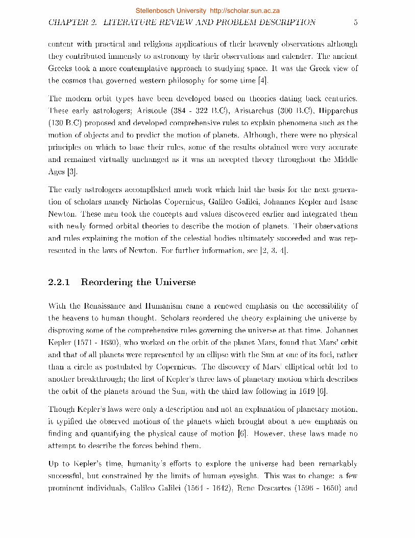
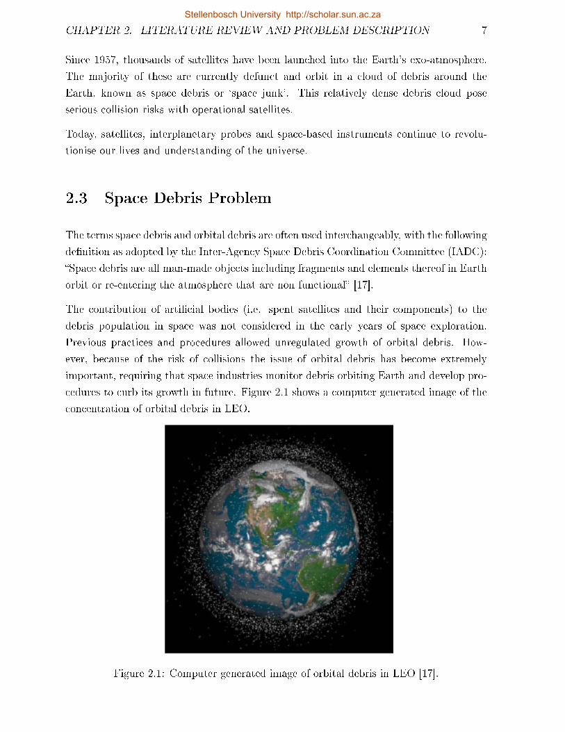
cedures to curb its growth in future. Figure 2.1 shows a computer generated image of the
concentration of orbital debris in LEO.
Figure 2.1: Computer generated image of orbital debris in LEO [17].
Stellenbosch University http://scholar.sun.ac.za
CHAPTER 2. LITERATURE REVIEW AND PROBLEM DESCRIPTION 8
Space debris is a problem of the near Earth environment with global dimensions to which
all spacefaring nations have contributed over more than half a century of space activities.
As the space debris environment evolved progressively, it became evident that understand-
ing its causes and controlling its sources are a prerequisite to ensure safe space ight [14].
In the past, the natural meteoroid environment was considered in satellite designs. Present
and future satellite designs have to take in account space debris in addition to the natural
environment. Past design practices, including deliberate and unintentional explosions in
space, have created a signicant debris population within the region of operationally im-
portant orbits [3]. Much of these debris are resident at altitudes of considerable operational
interest.
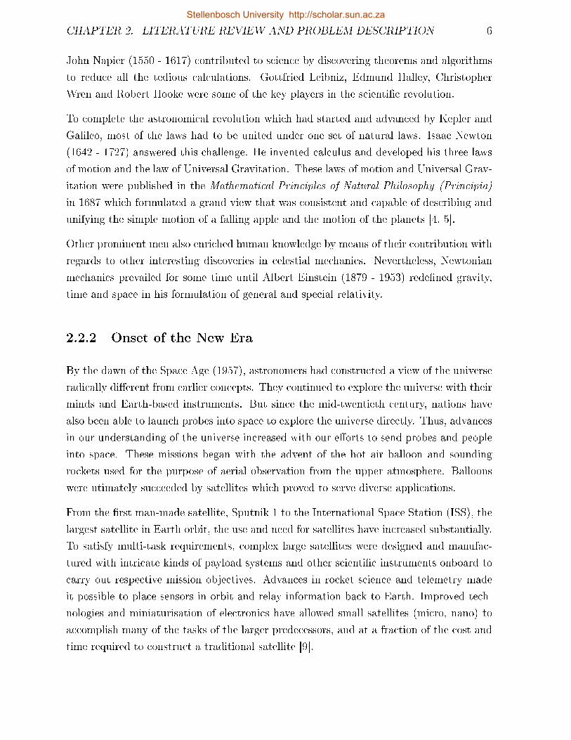
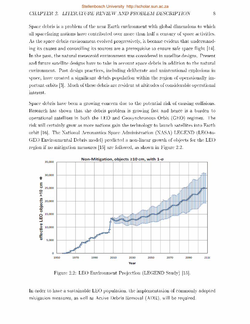
Space debris have been a growing concern due to the potential risk of causing collisions.
Research has shown that the debris problem is growing fast and hence is a burden to
operational satellites in both the LEO and Geosynchronous Orbit (GEO) regimes. The
risk will certainly grow as more nations gain the technology to launch satellites into Earth
orbit [16]. The National Aeronautics Space Administration (NASA) LEGEND (LEO-to-
GEO Environmental Debris model) predicted a non-linear growth of objects for the LEO
region if no mitigation measures [15] are followed, as shown in Figure 2.2.
Figure 2.2: LEO Environment Projection (LEGEND Study) [15].
In order to have a sustainable LEO population, the implementation of commonly adopted
mitigation measures, as well as Active Debris Removal (ADR), will be required.
Stellenbosch University http://scholar.sun.ac.za
CHAPTER 2. LITERATURE REVIEW AND PROBLEM DESCRIPTION 9
2.3.1 Concerns and Threats posed by Space Debris
The most important single source of debris proliferation is on-orbit collisions of satellites
and rocket stages, sometimes more than 20 years after their launch [14]. Collisions are
either accidental or deliberate. The Chinese shot down their satellite (deliberately) [35]
while an Iridium-Cosmos collision was accidental [43]. When these collisions happen they
also produce many fragments. The abandonment of satellites and upper stages in their
current orbit, after their operational lifetime, is also a major contributor to the space
population. These practises have led to the accumulation of approximately 1968 tons
of orbital debris as reported by NASA in 1995 [18]. The average growth rate in debris
population of about 5% per annum in LEO is as a result of assets being launched into
space at a faster rate than being removed by either articial or natural means.
Studies have shown that, even if there were no new launches, collisions of existing satellites
and rocket bodies would lead to a growing debris count as more pieces of debris are created
which in turn collide with each other. Therefore collisions will most likely be the largest
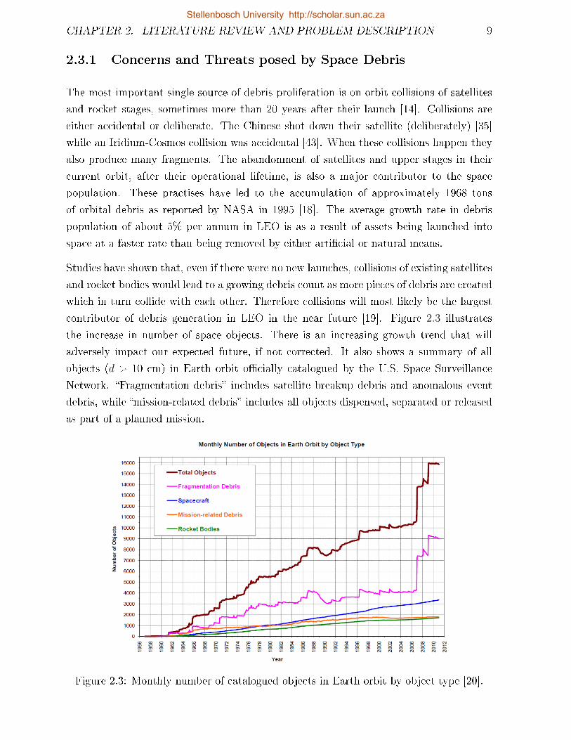
contributor of debris generation in LEO in the near future [19]. Figure 2.3 illustrates
the increase in number of space objects. There is an increasing growth trend that will
adversely impact our expected future, if not corrected. It also shows a summary of all
objects (d > 10 cm) in Earth orbit ocially catalogued by the U.S. Space Surveillance
Network. Fragmentation debris includes satellite breakup debris and anomalous event
debris, while mission-related debris includes all objects dispensed, separated or released
as part of a planned mission.
Figure 2.3: Monthly number of catalogued objects in Earth orbit by object type [20].
Stellenbosch University http://scholar.sun.ac.za
CHAPTER 2. LITERATURE REVIEW AND PROBLEM DESCRIPTION 10
The growth of space debris has become an issue of concern as it continues to have an
impact on the utilisation of space assets. This impacts both the immediate and long term
eects of collisions and explosions in the space debris population. The motivation for
this study is as a result of the growing concern about `space junk' and how it can be
controlled by means of deorbiting these satellites after their operational lifetime, hence
the requirement for lifetime predictions. Removal of some of these defunct satellites (e.g.
SUNSAT) in the LEO region, is the primary focus.
2.3.2 Mitigation Guidelines
Controlling the growth of the space debris population is a high priority for most major
spacefaring nations for future generations. Currently, the man-made debris environment
in the LEO region is assumed to dominate the natural meteoroid contribution, except for
a conned size regime around 0.1 mm diameter [21].
Mitigation measures take the form of preventing the creation of new debris, designing
satellites to withstand impacts by small debris and implementing operational procedures
such as using orbital regimes with less debris, adopting specic satellite attitudes and even
maneuvering to avoid collisions with debris.
Several orbital debris mitigation guidelines have been issued by various organisations -
NASA, U.S Government, the IADC and the Federal Communications Commission (FCC).
Some of these guidelines are summarised here shortly, with the focus on post mission
disposal of satellites in LEO for the purpose of this study.
NASA [22] have three main options for post mission disposal in LEO:
atmospheric re-entry,
maneuvering to storage orbits,
direct retrieval.
The U.S Government [23] have similar mitigation guidelines, but with some
additions in the various domains.
Option one includes the human casualty risk, which should be less than
one in ten thousand for re-entry into the Earth's atmosphere.
The second option discusses several storage regimes:
between LEO and MEO,
between MEO and GEO,
Stellenbosch University http://scholar.sun.ac.za
CHAPTER 2. LITERATURE REVIEW AND PROBLEM DESCRIPTION 11
Above GEO,
Heliocentric, Earth-escape.
The last option makes use of time constraints:
removal from orbit should be as soon as practical after completion of
a mission.
The IADC guidelines [17] give alternatives for space structures to be disposed
of by either deorbiting, direct re-entry, maneuvering to an orbit that reduces
the lifetime and nally by direct retrieval.
The FCC guidelines [24] comprise three dierent procedures for post mission
disposal similar to that of NASA, but with an addition in atmospheric re-entry:
use the propulsion system of a spacecraft to lower the orbit attitude to-
wards the Earth's atmosphere.
maneuver the satellite into an orbit where atmospheric drag will accel-
erate its re-entry, causing it to decay within 25 years after launch by
mechanically increasing the satellite's cross-sectional area.
A satellite system operator should submit a debris mitigation plan for authorisation to
enhance a continuous debris free environment as suggested by the FCC. For detailed
description of these mitigation guidelines, refer to the following papers [22, 23, 17, 24]
respectively.
2.4 DeOrbitSail Concept
A non-rocket form of space travel known as solar sailing was conceived by Tsiolkovsky [37]
and Tsander in the 1920's [38]. However, critical developments had to wait till the mid
seventies where a rendezvous mission was proposed making use of a solar sail, but was
later cancelled. Albeit, the study sparked international interest in solar sailing for future
mission applications [25].
Solar sailing is a means of travelling in space by using the energy from the Sun. It gains
momentum from photons, the quantum packets of energy of which sunlight is composed.
Solar sailing is a unique form of propellant-less propulsion reducing the reliance on a
reaction mass, such as chemical propulsion. As solar sails are not limited by a nite
reaction mass, they can provide continuous acceleration, limited only by the lifetime of
the sail lm in the space environment [26]. In order to generate as high an acceleration as
Stellenbosch University http://scholar.sun.ac.za
CHAPTER 2. LITERATURE REVIEW AND PROBLEM DESCRIPTION 12
possible from the momentum transported by the intercepted photons, solar sails must be
made extremely light and also near perfect reectors.
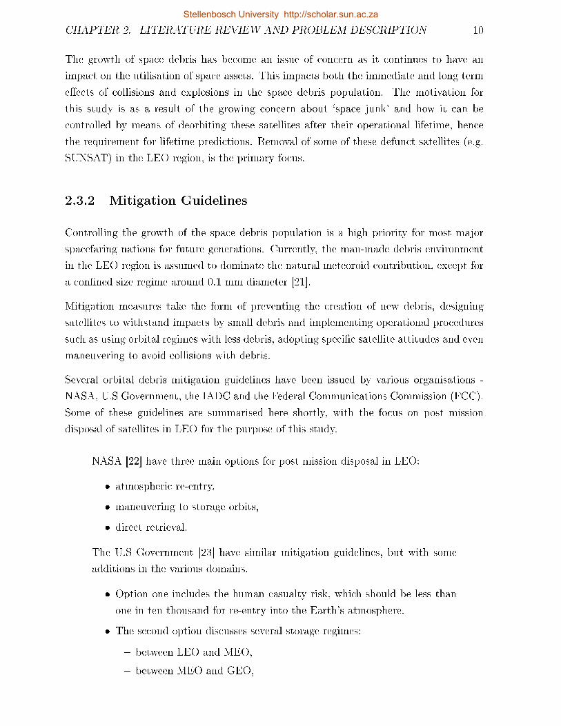
A solar sail is thus a large membrane of thin reective material which reects incident
photons from the Sun, thereby causing acceleration [27]. Solar sailing could be compared
to the sail of a ship, but using solar radiation pressure for propulsion instead of the wind.
Figure 2.4 shows a typical solar sail when deployed. For a comprehensive discussion on
the dynamics of a solar sail, orbit conguration and types, its performance and mission
related technologies, refer to [26, 27].
Figure 2.4: Typical deployed 1.7× 1.7m sail [28].
The DeOrbitSail mission [42] is to employ a drag sail as a deorbiting mechanism to augment
the proposed methods for debris mitigation. DeOrbitSail is a deorbiting device that uses
aerodynamic drag for deorbiting. It is very low in complexity, has a low parasitic mass
and does not require any propellant. The purpose of the drag sail is to demonstrate and
prove the eectiveness of drag deorbiting, by increasing the drag area and shortening the
orbit decay period. Solar radiation pressure can also be used for the general maneuvering
of satellites to higher or lower orbits. Solar sailing is more eective above about 650 km
when the constant solar force becomes more dominant than the drag force and below 650
km the drag force becomes exponentially more dominant.
Investigations have shown that the use of a solar or drag sail as a deorbiting mechanism
can be an advantageous, low-cost solution for deorbiting satellites, as the total cost of
the technology is not prohibitive. For certain missions, it can be a better solution than
Stellenbosch University http://scholar.sun.ac.za
CHAPTER 2. LITERATURE REVIEW AND PROBLEM DESCRIPTION 13
a traditional chemical propulsion system, which would require large amounts of chemical
propellant [28].
The solar sail technology was employed on the interplanetary IKAROS satellite launched in
May, 2010. With a 200 m2 sail, its objective was to demonstrate the solar sailing principle
[29]. Though the solar sail had been successfully deployed, its overall eectiveness and
success still need to be assessed. The orbital lifetime of Nanosail-D2 (240 days) showed the
eciency of the drag sail technology [39]. The benets and capabilities of solar and drag
sailing as a means of deorbiting still requires further investigation, hence the motivation
for this study.
Evaluation of the potential risk involved with space debris have led to possible solutions
and reduction measures such as the deorbitsail concept. Active removal of defunct space-
craft, upper stages and other space junk may be the most ecient means of avoiding
future collisions. However, it might not be cost eective and would require dicult ma-
neuvering of objects in space.
2.5 Summary
This chapter provides a description of the history leading to the dawn of the space age. A
brief overview of the historical foundation is discussed. The space debris problem with an
outline of some proposed mitigation guidelines are presented. These guidelines cover the
overall environmental impact of space missions with a focus on the following: limitation
of debris released during normal operations, minimisation of the potential for on-orbit
break-ups, prevention of on-orbit collisions and post-mission disposal (which is the main
aim of this study).
Recent events have accentuate the growing problem that orbital debris, or space junk
poses to spacecraft. In order to control this problem, the idea of the deorbitsail concept
is proposed and described. This seeks to demonstrate satellite deorbiting manoeuvres for
space debris mitigation and to reduce the deorbit time of satellites by increasing the drag
area.
Stellenbosch University http://scholar.sun.ac.za
Chapter 3
Theoretical Background
3.1 Introduction
Understanding the motion of an object in space is fundamental to orbit propagation and
determination. In this chapter, the necessary theory and concepts of orbital mechanics
using the equations of motion for two-body and N-body problems are introduced. Detailed
analyses, solution or implementation of the two-body or N-body problem, however, falls
outside the scope of this study and are not addressed.
Relevant coordinate frames used in this work are discussed. The transformation matrices
employed to convert coordinates from one reference frame to another are presented. Be-
cause of the importance of historic Two-Line Element data used in the study, this topic
is addressed in some detail, but the popular Simplied General Pertubation (SGP4) orbit
propagator [13] is not covered.
3.2 Equations of Motion
Orbital equations of motion are governed by Kepler and Newton's laws. Kepler's laws
describe the motion of planets in the solar system and can be applied to articial Earth
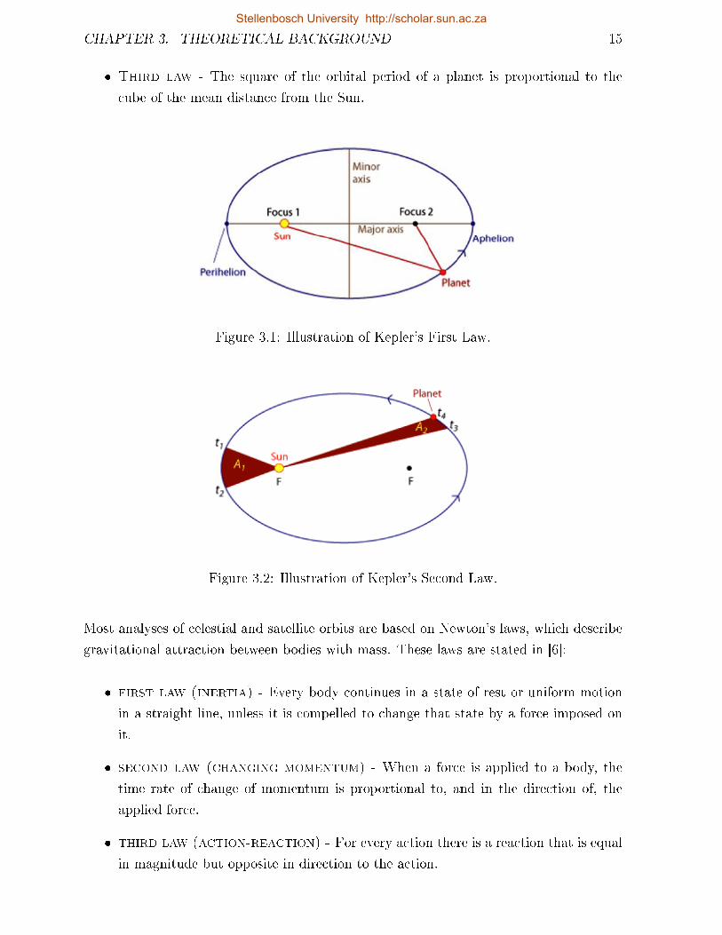
satellite motion as well. Kepler's laws are illustrated in Figures 3.1 and 3.2 and in [6]:
First law - The orbits of the planets are ellipses with the Sun at one focus.
Second law - The line joining the planet to the Sun sweeps out equal areas in
equal times.
14
Stellenbosch University http://scholar.sun.ac.za
CHAPTER 3. THEORETICAL BACKGROUND 15
Third law - The square of the orbital period of a planet is proportional to the
cube of the mean distance from the Sun.
Figure 3.1: Illustration of Kepler's First Law.
Figure 3.2: Illustration of Kepler's Second Law.
Most analyses of celestial and satellite orbits are based on Newton's laws, which describe
gravitational attraction between bodies with mass. These laws are stated in [6]:
first law (inertia) - Every body continues in a state of rest or uniform motion
in a straight line, unless it is compelled to change that state by a force imposed on
it.
second law (changing momentum) - When a force is applied to a body, the
time rate of change of momentum is proportional to, and in the direction of, the
applied force.
third law (action-reaction) - For every action there is a reaction that is equal
in magnitude but opposite in direction to the action.
Stellenbosch University http://scholar.sun.ac.za
CHAPTER 3. THEORETICAL BACKGROUND 16
law of universal gravitation - Every particle in the universe attracts every
other particle with a force that is proportional to the product of the masses and
inversely proportional to the square of the distance between the particles.
3.2.1 Two-Body Equation
3.2.1.1 Assumptions
In developing the two-body equation, certain assumptions are made [4]:
1. The bodies of the satellite and attracting body are spherically symmetrical with
uniform density, hence can be considered as point masses.
2. The coordinate system chosen for a particular problem is inertial. The geocentric
equatorial system serves for satellites orbiting the Earth.
3. No external forces act on the system except for the gravitational forces that act
along a line joining the centers of the two bodies.
3.2.1.2 Equation of Relative Motion
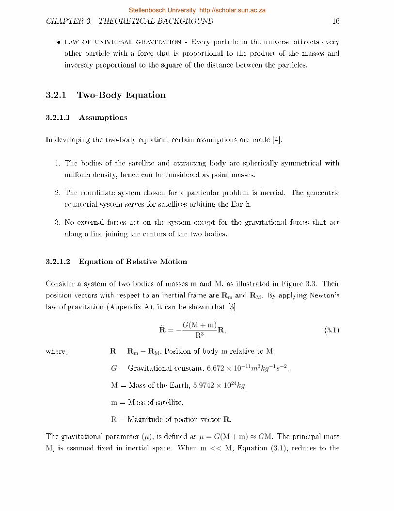
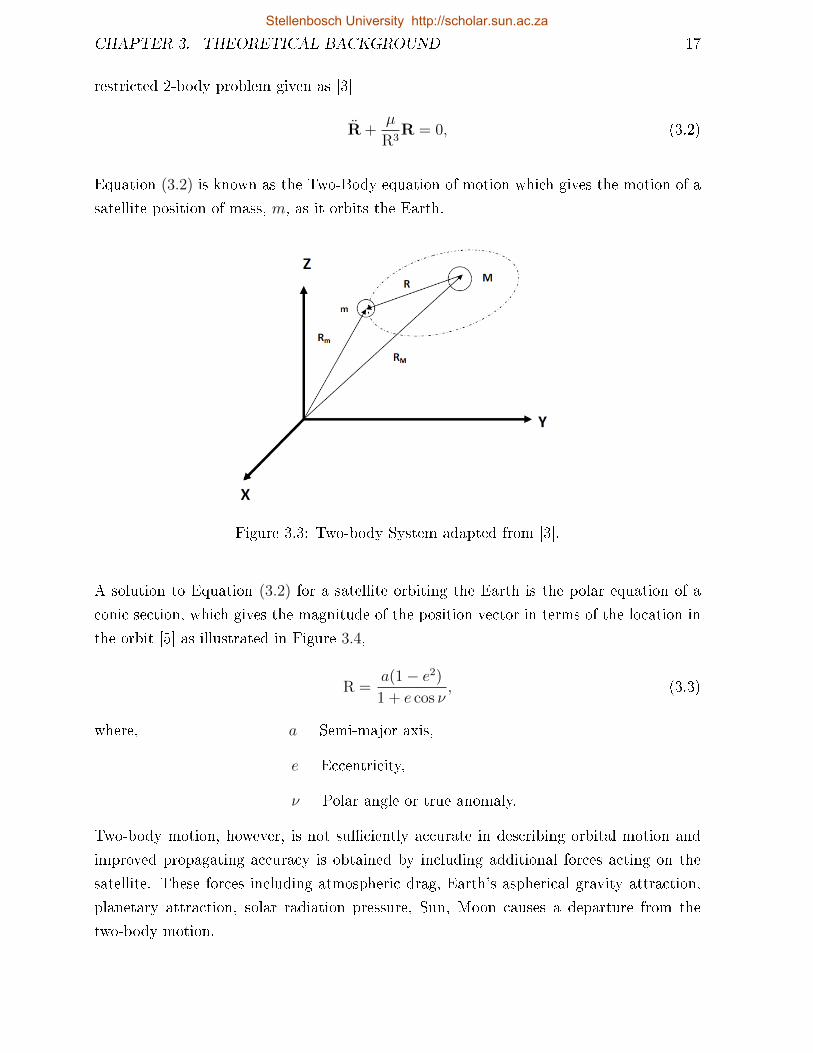
Consider a system of two bodies of masses m and M, as illustrated in Figure 3.3. Their
position vectors with respect to an inertial frame are Rm and RM. By applying Newton's
law of gravitation (Appendix A), it can be shown that [3]
R = −G(M + m)
R3R, (3.1)
where, R = Rm −RM, Position of body m relative to M,
G = Gravitational constant, 6.672× 10⁻¹¹m3kg−1s−2,
M = Mass of the Earth, 5.9742× 1024kg,
m = Mass of satellite,
R = Magnitude of postion vector R.
The gravitational parameter (µ), is dened as µ = G(M + m) ≈ GM. The principal mass
M, is assumed xed in inertial space. When m << M, Equation (3.1), reduces to the
Stellenbosch University http://scholar.sun.ac.za
CHAPTER 3. THEORETICAL BACKGROUND 17
restricted 2-body problem given as [3]
R +µ
R3R = 0, (3.2)
Equation (3.2) is known as the Two-Body equation of motion which gives the motion of a
satellite position of mass, m, as it orbits the Earth.
Figure 3.3: Two-body System adapted from [3].
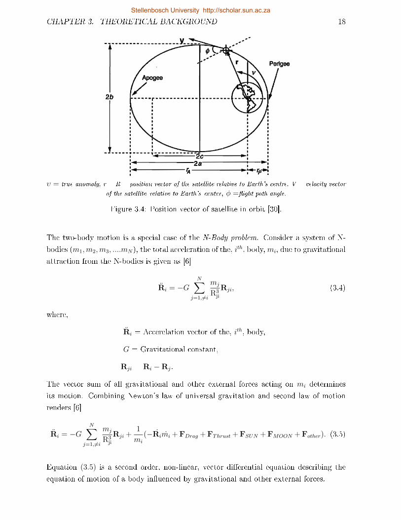
A solution to Equation (3.2) for a satellite orbiting the Earth is the polar equation of a
conic section, which gives the magnitude of the position vector in terms of the location in
the orbit [5] as illustrated in Figure 3.4,
R =a(1− e2)
1 + e cos ν, (3.3)
where, a = Semi-major axis,
e = Eccentricity,
ν = Polar angle or true anomaly.
Two-body motion, however, is not suciently accurate in describing orbital motion and
improved propagating accuracy is obtained by including additional forces acting on the
satellite. These forces including atmospheric drag, Earth's aspherical gravity attraction,
planetary attraction, solar radiation pressure, Sun, Moon causes a departure from the
two-body motion.
Stellenbosch University http://scholar.sun.ac.za
CHAPTER 3. THEORETICAL BACKGROUND 18
υ = true anomaly, r = R = position vector of the satellite relative to Earth's centre, V = velocity vector
of the satellite relative to Earth's center, φ =ight path angle.
Figure 3.4: Position vector of satellite in orbit [30].
The two-body motion is a special case of the N-Body problem. Consider a system of N-
bodies (m1,m2,m3, ....mN), the total acceleration of the, ith, body,mi, due to gravitational
attraction from the N-bodies is given as [6]
Ri = −GN∑
j=1,6=i
mj
R3ji
Rji, (3.4)
where,
Ri = Accerelation vector of the, ith, body,
G = Gravitational constant,
Rji = Ri −Rj.
The vector sum of all gravitational and other external forces acting on mi determines
its motion. Combining Newton's law of universal gravitation and second law of motion
renders [6]
Ri = −GN∑
j=1,6=i
mj
R3ji
Rji +1
mi
(−Rimi + FDrag + FThrust + FSUN + FMOON + Fother). (3.5)
Equation (3.5) is a second order, non-linear, vector dierential equation describing the
equation of motion of a body inuenced by gravitational and other external forces.
Stellenbosch University http://scholar.sun.ac.za
CHAPTER 3. THEORETICAL BACKGROUND 19
The N-body problem is a coupled second order dierential equation which has to be
solved numerically by numerical integration using high-order numerical integrators such
as Runge-Kutta, Adams-Bashforth-Moulton, Gauss-Jackson [4] etc. to achieve precision
and medium term orbit propagation results. However, this is not the scope of the study
and hence will not be addressed in detail.
SALT utilises the eect of Earth's aspherical gravity and atmospheric drag, hence these
perturbations will be discussed in detail in Chapter 4.
3.2.2 Constants of Motion
Orbital motion occurs in a conservative gravitational eld which explains why satellites
conserve mechanical energy and angular momentum.
3.2.2.1 Energy Law
The energy constant of motion is obtained by scalar multiplication of Equation (3.2) by
R. After some manipulation, the conservation of energy, namely the specic mechanical
energy (Appendix A) is found as [5]:
V 2
2− µ
R= ε = constant, (3.6)
with, ε = Satellite's specic mechanical energy = -µ
2a(km2/s2),
V = Satellite's velocity (km/s),
µ = Gravitational parameter (km3/s2),
R = Satellite's distance from Earth's centre (km).
The relative kinetic energy per unit mass isV 2
2and −µ
Ris the potential energy per unit
mass of a satellite. The total mechanical energy per unit mass (ε), is the sum of the
kinetic and potential energies per unit mass. Because ε is conserved, it must be the same
at any point along an orbit. Specic mechanical energy (ε) is dependent on position (R),
velocity (V) and the local gravitational parameter (µ). Hence if the position and velocity
of a satellite along any point on the orbit is known, the specic mechanical energy at every
point on its orbit is also known. Equation (3.6) is also referred to as the energy integral
or the vis− viva equation. It is valid for all trajectories, including rectilinear ones.
Stellenbosch University http://scholar.sun.ac.za
CHAPTER 3. THEORETICAL BACKGROUND 20
3.2.2.2 Angular Momentum
Angular momentum is very useful in determining and maintaining the satellite's orbit.
The angular momentum constant of motion for a satellite is the result of the cross product
between the position and velocity vectors. This is evaluated by cross-multiplying Equation
(3.2) by R (Appendix A). The resultant is the specic angular momentum h, given as [5]
h = R×V, (3.7)
where h = Satellite's specic angular momentum vector (km2/s),
R = Satellite's position vector (km),
V = Satellite's velocity vector (km/s).
The angular momentum vector (h) is always perpendicular to (R) and (V), which denes
the orbital plane. Thus if h is at right angles to the orbital plane and it is a constant,
then the orbital plane must also be constant. In Equation (3.2) the orbital plane is forever
frozen in inertial space. In reality, due to orbit perturbations, the orbital plane changes
gradually over time.
3.2.2.3 Trajectory Equation
The trajectory equation presents a great insight into orbital motion, thus describing the
dimensions and shape of the orbit. By writing equation (3.2) into the specic angular
momentum vector h and evaluating, we nd the actual solution for a satellite's motion in
polar coordinates as Equation (3.3) [4] with p = a(1− e2), where p is the semiparameter
and e the eccentricity which denes the shape of the orbit as shown in the Table 3.1. The
trajectory equation doesn't restrict the motion of an ellipse, hence it's an extention of
Kepler's rst law as stated above.
Table 3.1: Relationship between conic section and eccentricity.
Conic Section Eccentricity (e)Circle e = 0Ellipse 0 < e < 1Parabola e = 1Hyperbola e > 1
Stellenbosch University http://scholar.sun.ac.za
CHAPTER 3. THEORETICAL BACKGROUND 21
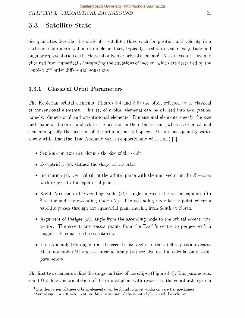
3.3 Satellite State
Six quantities describe the orbit of a satellite, three each for position and velocity in a
cartesian coordinate system or an element set, typically used with scalar magnitude and
angular representation of the classical or Kepler orbital elements1. A state vector is usually
obtained from numerically integrating the equations of motion, which are described by the
coupled 2nd order dierential equations.
3.3.1 Classical Orbit Parameters
The Keplerian orbital elements (Figures 3.4 and 3.5) are often referred to as classical
or conventional elements. This set of orbital elements can be divided into two groups,
namely: dimensional and orientational elements. Dimensional elements specify the size
and shape of the orbit and relate the position in the orbit to time, whereas orientational
elements specify the position of the orbit in inertial space. All but one quantity varies
slowly with time (the True Anomaly varies proportionally with time) [3].
Semi-major Axis (a): denes the size of the orbit.
Eccentricity (e): denes the shape of the orbit.
Inclination (i): vertical tilt of the orbital plane with the unit vector in the Z − axiswith respect to the equatorial plane.
Right Ascension of Ascending Node (Ω): angle between the vernal equinox (Υ)2 vector and the ascending node (N). The ascending node is the point where a
satellite passes through the equatorial plane moving from South to North.
Argument of Perigee (ω): angle from the ascending node to the orbital eccentricity
vector. The eccentricity vector points from the Earth's centre to perigee with a
magntitude equal to the eccentricity.
True Anomaly (ν): angle from the eccentricity vector to the satellite position vector.
Mean anomaly (M ) and eccentric anomaly (E ) are also used in calculation of orbit
parameters.
The rst two elements dene the shape and size of the ellipse (Figure 3.4). The parameters,
i and Ω dene the orientation of the orbital plane with respect to the coordinate system
1The derivation of these orbital elements can be found in most works on celestial mechanics.2Vernal equinox - It is a point on the intersection of the celestial plane and the ecliptic.
Stellenbosch University http://scholar.sun.ac.za
CHAPTER 3. THEORETICAL BACKGROUND 22
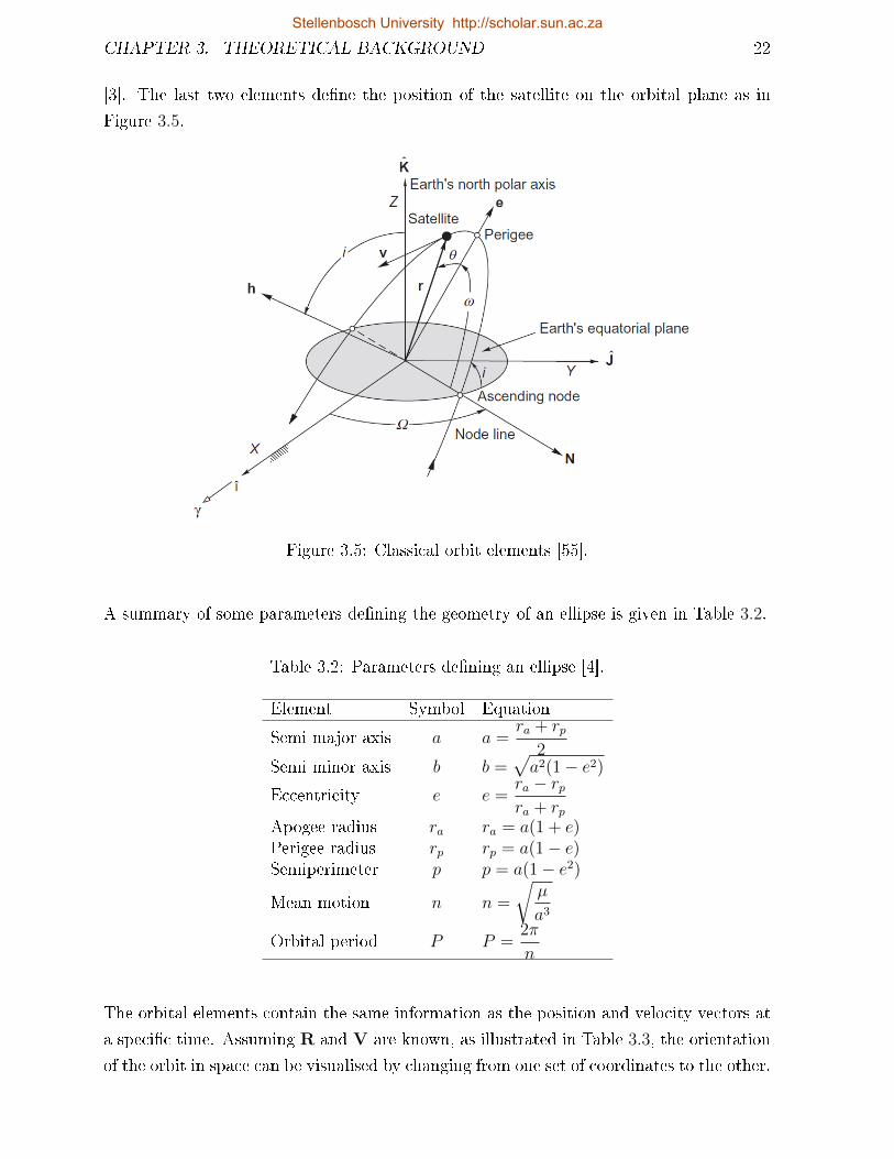
[3]. The last two elements dene the position of the satellite on the orbital plane as in
Figure 3.5.
Figure 3.5: Classical orbit elements [55].
A summary of some parameters dening the geometry of an ellipse is given in Table 3.2.
Table 3.2: Parameters dening an ellipse [4].
Element Symbol Equation
Semi major axis a a =ra + rp
2Semi minor axis b b =
√a2(1− e2)
Eccentricity e e =ra − rpra + rp
Apogee radius ra ra = a(1 + e)Perigee radius rp rp = a(1− e)Semiperimeter p p = a(1− e2)
Mean motion n n =
õ
a3
Orbital period P P =2π
n
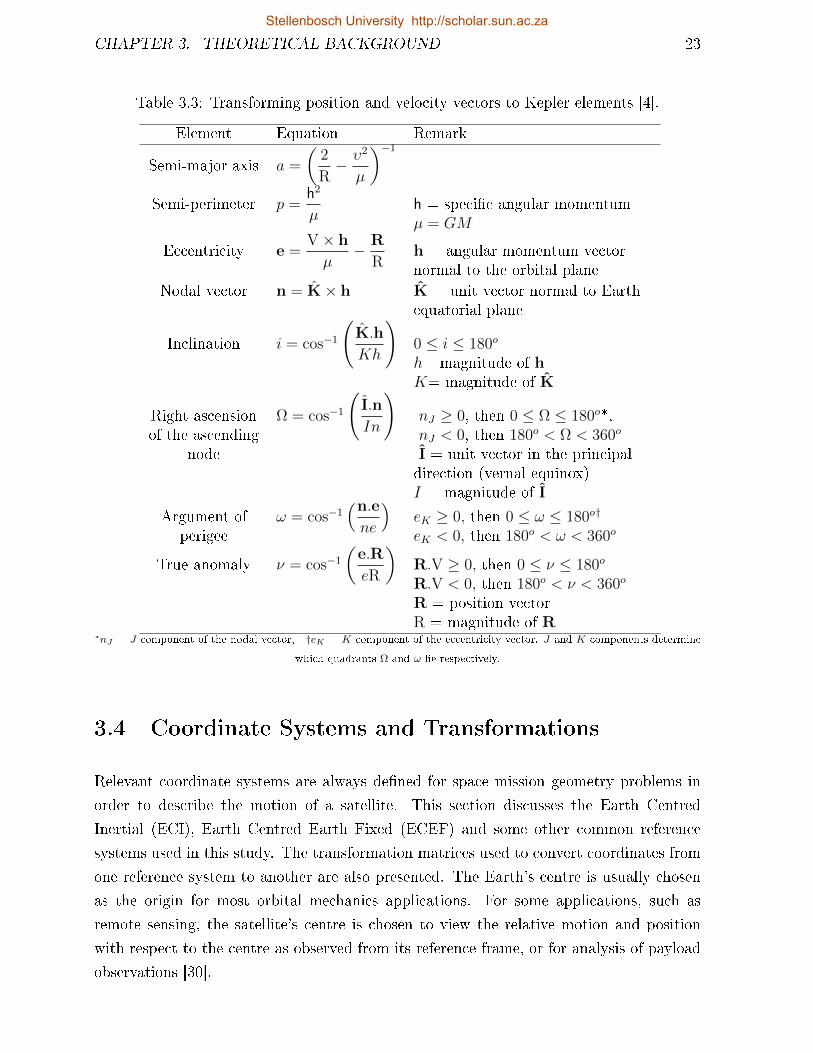
The orbital elements contain the same information as the position and velocity vectors at
a specic time. Assuming R and V are known, as illustrated in Table 3.3, the orientation
of the orbit in space can be visualised by changing from one set of coordinates to the other.
Stellenbosch University http://scholar.sun.ac.za
CHAPTER 3. THEORETICAL BACKGROUND 23
Table 3.3: Transforming position and velocity vectors to Kepler elements [4].
Element Equation Remark
Semi-major axis a =
(2
R− υ2
µ
)−1
Semi-perimeter p =h2
µh = specic angular momentumµ = GM
Eccentricity e =V × h
µ− R
Rh = angular momentum vectornormal to the orbital plane
Nodal vector n = K× h K = unit vector normal to Earthequatorial plane
Inclination i = cos−1
(K.h
Kh
)0 ≤ i ≤ 180o
h= magnitude of hK= magnitude of K
Right ascensionof the ascending
node
Ω = cos−1
(I.n
In
)nJ ≥ 0, then 0 ≤ Ω ≤ 180o*,nJ < 0, then 180o < Ω < 360o
I = unit vector in the principaldirection (vernal equinox)I = magnitude of I
Argument ofperigee
ω = cos−1(n.e
ne
)eK ≥ 0, then 0 ≤ ω ≤ 180o†
eK < 0, then 180o < ω < 360o
True anomaly ν = cos−1
(e.R
eR
)R.V ≥ 0, then 0 ≤ ν ≤ 180o
R.V < 0, then 180o < ν < 360o
R = position vectorR = magnitude of R
*nJ = J component of the nodal vector, †eK = K component of the eccentricity vector. J and K components determine
which quadrants Ω and ω lie respectively.
3.4 Coordinate Systems and Transformations
Relevant coordinate systems are always dened for space mission geometry problems in
order to describe the motion of a satellite. This section discusses the Earth Centred
Inertial (ECI), Earth Centred Earth Fixed (ECEF) and some other common reference
systems used in this study. The transformation matrices used to convert coordinates from
one reference system to another are also presented. The Earth's centre is usually chosen
as the origin for most orbital mechanics applications. For some applications, such as
remote sensing, the satellite's centre is chosen to view the relative motion and position
with respect to the centre as observed from its reference frame, or for analysis of payload
observations [30].
Stellenbosch University http://scholar.sun.ac.za
CHAPTER 3. THEORETICAL BACKGROUND 24
3.4.1 Reference Systems
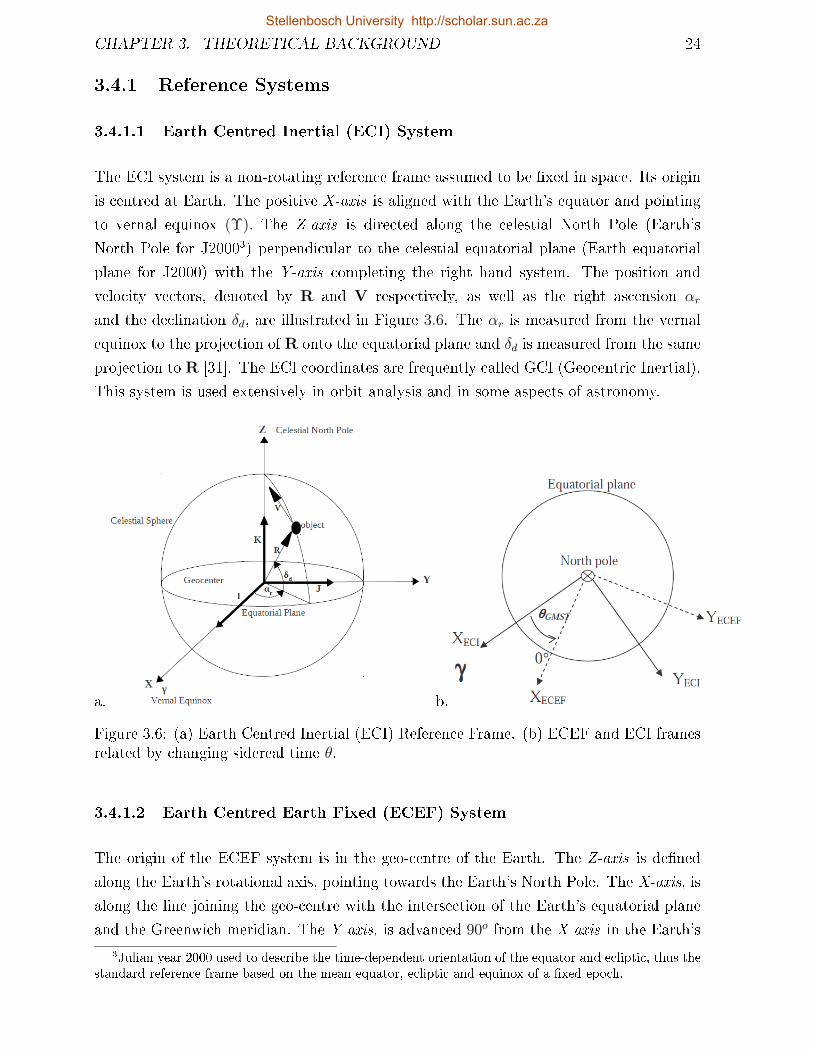
3.4.1.1 Earth Centred Inertial (ECI) System
The ECI system is a non-rotating reference frame assumed to be xed in space. Its origin
is centred at Earth. The positive X-axis is aligned with the Earth's equator and pointing
to vernal equinox (Υ). The Z-axis is directed along the celestial North Pole (Earth's
North Pole for J20003) perpendicular to the celestial equatorial plane (Earth equatorial
plane for J2000) with the Y-axis completing the right hand system. The position and
velocity vectors, denoted by R and V respectively, as well as the right ascension αr
and the declination δd, are illustrated in Figure 3.6. The αr is measured from the vernal
equinox to the projection of R onto the equatorial plane and δd is measured from the same
projection to R [31]. The ECI coordinates are frequently called GCI (Geocentric Inertial).
This system is used extensively in orbit analysis and in some aspects of astronomy.
a. b.
Figure 3.6: (a) Earth Centred Inertial (ECI) Reference Frame. (b) ECEF and ECI framesrelated by changing sidereal time θ.
3.4.1.2 Earth Centred Earth Fixed (ECEF) System
The origin of the ECEF system is in the geo-centre of the Earth. The Z-axis is dened
along the Earth's rotational axis, pointing towards the Earth's North Pole. The X-axis, is
along the line joining the geo-centre with the intersection of the Earth's equatorial plane
and the Greenwich meridian. The Y-axis, is advanced 90o from the X-axis in the Earth's
3Julian year 2000 used to describe the time-dependent orientation of the equator and ecliptic, thus thestandard reference frame based on the mean equator, ecliptic and equinox of a xed epoch.
Stellenbosch University http://scholar.sun.ac.za
CHAPTER 3. THEORETICAL BACKGROUND 25
equatorial plane. The ECEF coordinate rotates with the Earth about its rotation axis
[4]. It's very useful in processing satellite observations from a site and conversion of actual
observations to the J2000 system for use in other calculations. The ECEF and ECI frames
are related through the Greenwich mean sidereal time θGMST as in Figure 3.6b.
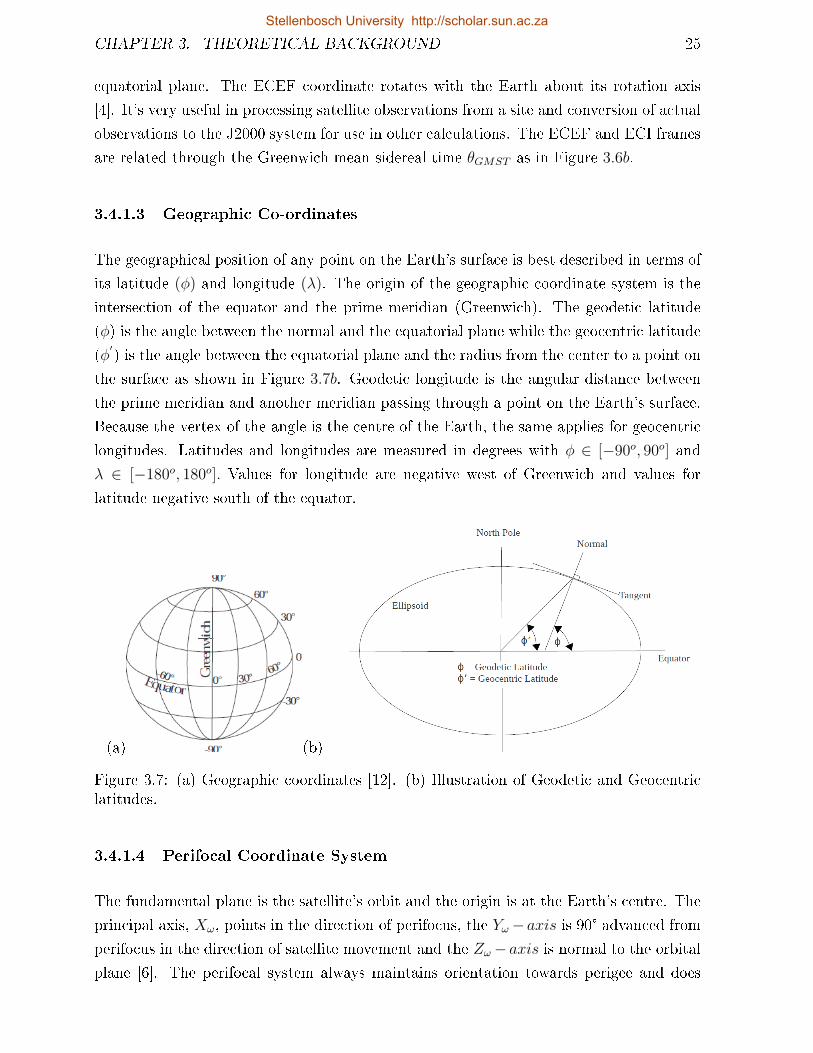
3.4.1.3 Geographic Co-ordinates
The geographical position of any point on the Earth's surface is best described in terms of
its latitude (φ) and longitude (λ). The origin of the geographic coordinate system is the
intersection of the equator and the prime meridian (Greenwich). The geodetic latitude
(φ) is the angle between the normal and the equatorial plane while the geocentric latitude
(φ′) is the angle between the equatorial plane and the radius from the center to a point on
the surface as shown in Figure 3.7b. Geodetic longitude is the angular distance between
the prime meridian and another meridian passing through a point on the Earth's surface.
Because the vertex of the angle is the centre of the Earth, the same applies for geocentric
longitudes. Latitudes and longitudes are measured in degrees with φ ∈ [−90o, 90o] and
λ ∈ [−180o, 180o]. Values for longitude are negative west of Greenwich and values for
latitude negative south of the equator.
(a) (b)
Figure 3.7: (a) Geographic coordinates [12]. (b) Illustration of Geodetic and Geocentriclatitudes.
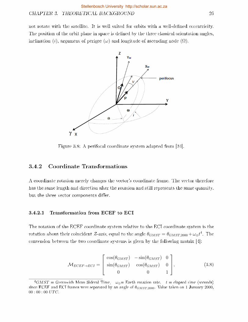
3.4.1.4 Perifocal Coordinate System
The fundamental plane is the satellite's orbit and the origin is at the Earth's centre. The
principal axis, Xω, points in the direction of perifocus, the Yω− axis is 90° advanced from
perifocus in the direction of satellite movement and the Zω− axis is normal to the orbitalplane [6]. The perifocal system always maintains orientation towards perigee and does
Stellenbosch University http://scholar.sun.ac.za
CHAPTER 3. THEORETICAL BACKGROUND 26
not rotate with the satellite. It is well suited for orbits with a well-dened eccentricity.
The position of the orbit plane in space is dened by the three classical orientation angles,
inclination (i), argument of perigee (ω) and longitude of ascending node (Ω).
Figure 3.8: A perifocal coordinate system adapted from [34].
3.4.2 Coordinate Transformations
A coordinate rotation merely changes the vector's coordinate frame. The vector therefore
has the same length and direction after the rotation and still represents the same quantity,
but the three vector components dier.
3.4.2.1 Transformation from ECEF to ECI
The rotation of the ECEF coordinate system relative to the ECI coordinate system is the
rotation about their coincident Z-axis, equal to the angle θGMST = θGMST,2000 +ω⊕t4. The
conversion between the two coordinate systems is given by the following matrix [4]:
MECEF→ECI =
cos(θGMST ) − sin(θGMST ) 0
sin(θGMST ) cos(θGMST ) 0
0 0 1
, (3.8)
4GMST = Greenwich Mean Sideral Time, ω⊕= Earth rotation rate, t = elapsed time (seconds)since ECEF and ECI frames were separated by an angle of θGMST,2000. Value taken on 1 January 2000,00 : 00 : 00 UTC.
Stellenbosch University http://scholar.sun.ac.za
CHAPTER 3. THEORETICAL BACKGROUND 27
where, ω⊕ = 7.2921158553× 10⁻⁵ rad/s,
θGMST,2000 = 1.74476716333061 rad.
This conversion assumes that any precession, nutation and polar motion eects are ne-
glected. The same procedure is used for the inverse transformation, but with using the
transpose of the rotation matrix given above as it's an orthonormal matrix for which the
inverse equals the transpose.
3.4.2.2 Transformation between Perifocal Coordinates and ECI
The transformation from perifocal to ECI coordinate system can be used to nd R and
V of a satellite in the ECI system. Assuming a satellite is rotating in a counterclockwise
direction when viewed from Earth's North Pole, then the transformation from perifocal to
ECI can be made using three consecutive clockwise rotations by Euler angles5 conforming
to the 313 sequence (Figure 3.9). The rotation sequence follows as [31]
1. rotation about h mapping e onto I, 0 ≤ ω ≤ 2π,
2. rotation about I mapping h onto z, 0 ≤ i ≤ π,
3. rotation about z mapping I onto x, 0 ≤ Ω ≤ 2π.
The composite rotation tranforming a vector from perifocal to ECI coordinate system is
given as
RECIperifocal(ω, i,Ω) = R3(Ω, z)R2(i, I)R1(ω, h). (3.9)
Evaluating (3.9) gives the Direction Cosine Matrix (DCM)6 [31]
RECIperifocal(ω, i,Ω) =
c(Ω)c(ω)− s(Ω)s(ω)c(i) c(Ω)s(ω) + s(Ω)c(ω)c(i) s(Ω)s(i)
−s(Ω)c(ω)− c(Ω)s(ω)c(i) −s(Ω)s(ω) + c(Ω)c(ω)c(i) c(Ω)s(i)
s(ω)s(i) −c(ω)s(i) c(i)
,(3.10)
where c = cos and s = sin.
The inverse transformation i.e. from ECI to perifocal system can be obtained using the
inverse (transpose) of the DCM above.
5Euler theorem - the most general displacement of a rigid body with one point xed is a rotation aboutsome axis.
6DCM expresses one set of orthonormal basis vectors in terms of another set, or expresses a knownvector in a dierent basis.
Stellenbosch University http://scholar.sun.ac.za
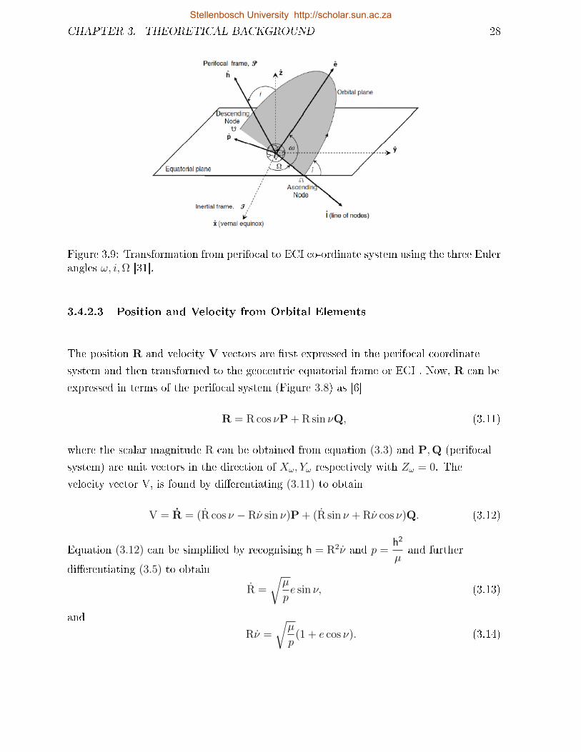
CHAPTER 3. THEORETICAL BACKGROUND 28
Figure 3.9: Transformation from perifocal to ECI co-ordinate system using the three Eulerangles ω, i,Ω [31].
3.4.2.3 Position and Velocity from Orbital Elements
The position R and velocity V vectors are rst expressed in the perifocal coordinate
system and then transformed to the geocentric equatorial frame or ECI . Now, R can be
expressed in terms of the perifocal system (Figure 3.8) as [6]
R = R cos νP + R sin νQ, (3.11)
where the scalar magnitude R can be obtained from equation (3.3) and P,Q (perifocal
system) are unit vectors in the direction of Xω, Yω respectively with Zω = 0. The
velocity vector V, is found by dierentiating (3.11) to obtain
V = R = (R cos ν − Rν sin ν)P + (R sin ν + Rν cos ν)Q. (3.12)
Equation (3.12) can be simplied by recognising h = R2ν and p =h2
µand further
dierentiating (3.5) to obtain
R =
õ
pe sin ν, (3.13)
and
Rν =
õ
p(1 + e cos ν). (3.14)
Stellenbosch University http://scholar.sun.ac.za
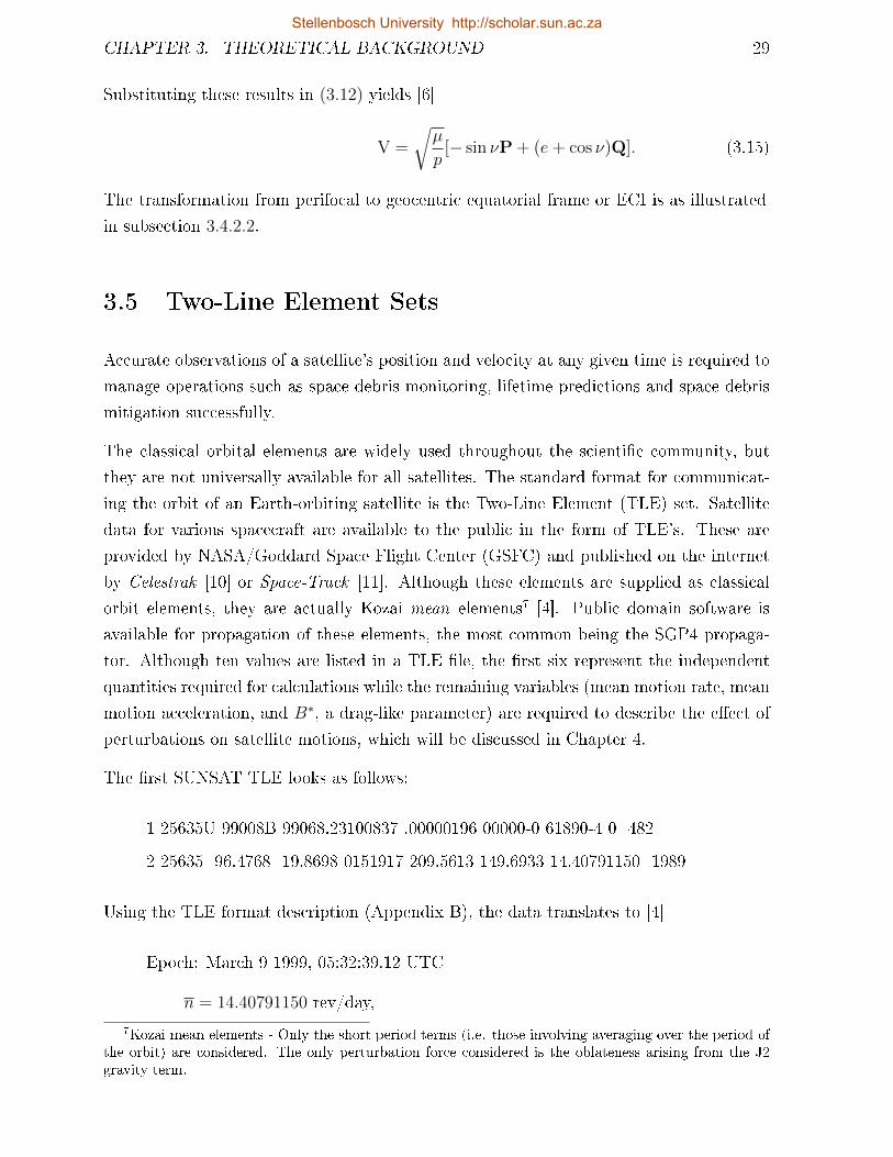
CHAPTER 3. THEORETICAL BACKGROUND 29
Substituting these results in (3.12) yields [6]
V =
õ
p[− sin νP + (e+ cos ν)Q]. (3.15)
The transformation from perifocal to geocentric equatorial frame or ECI is as illustrated
in subsection 3.4.2.2.
3.5 Two-Line Element Sets
Accurate observations of a satellite's position and velocity at any given time is required to
manage operations such as space debris monitoring, lifetime predictions and space debris
mitigation successfully.
The classical orbital elements are widely used throughout the scientic community, but
they are not universally available for all satellites. The standard format for communicat-
ing the orbit of an Earth-orbiting satellite is the Two-Line Element (TLE) set. Satellite
data for various spacecraft are available to the public in the form of TLE's. These are
provided by NASA/Goddard Space Flight Center (GSFC) and published on the internet
by Celestrak [10] or Space-Track [11]. Although these elements are supplied as classical
orbit elements, they are actually Kozai mean elements7 [4]. Public domain software is
available for propagation of these elements, the most common being the SGP4 propaga-
tor. Although ten values are listed in a TLE le, the rst six represent the independent
quantities required for calculations while the remaining variables (mean motion rate, mean
motion acceleration, and B∗, a drag-like parameter) are required to describe the eect of
perturbations on satellite motions, which will be discussed in Chapter 4.
The rst SUNSAT TLE looks as follows:
1 25635U 99008B 99068.23100837 .00000196 00000-0 61890-4 0 482
2 25635 96.4768 19.8698 0151917 209.5613 149.6933 14.40791150 1989
Using the TLE format description (Appendix B), the data translates to [4]
Epoch: March 9 1999, 05:32:39.12 UTC
n = 14.40791150 rev/day,
7Kozai mean elements - Only the short period terms (i.e. those involving averaging over the period ofthe orbit) are considered. The only perturbation force considered is the oblateness arising from the J2gravity term.
Stellenbosch University http://scholar.sun.ac.za
CHAPTER 3. THEORETICAL BACKGROUND 30
n
2= 1.96× 10⁻⁶ rev/day2,
n
6= 0.0 rev/day3,
B∗ = 6.1890× 10⁵,
e = 0.0151917,
i = 96.4768o,
Ω = 19.8698o,
ω = 209.5613o,
M = 149.6933o.
The true ballistic coecient BC, is obtained from B∗ with a constant conversion of [32]
BC =1
12.74162B∗kg.m−2.
However, the value of B∗ is always modied. It is an arbitrary free parameter in the
dierential correction [4].
3.6 Summary
The equations described in this chapter exemplies the two-body problem, though not
suciently accurate for satellite ephemerides or for calculations which requires precise
knowledge of the satellite's position or velocity. However, they are accurate enough to
estimate overall mission characteristics in most regions of space.
The requirement for describing an orbit is to dene a suitable reference frame, thus nding
an appropriate inertial coordinate system. A description of the coordinate frames used in
this study is presented. The position of the satellite is best described in terms of the Earth
Centred Inertial (ECI) frame. The dierent transformation matrices needed to convert
from one coordinate frame to the other is addressed. Data in the form of TLE's obtained
from [10, 11] are used extensively in this study, hence a description of the two-line element
set is presented and further explained in Appendix B.
The following chapter describes the importance of SALT and its application in LIFTIM for
this study. The equations of motion and the perturbative eects on the orbital elements
are presented.
Stellenbosch University http://scholar.sun.ac.za
Chapter 4
Orbit Perturbations and Decay
Employed in SALT
4.1 Introduction
Analytic solutions which describes the eect of atmospheric drag on the motion of articial
satellites exist. But these solutions are usually based on simplied analytical models for
the atmospheric density and also have some limitations on the size of the eccentricity
and/or the perigee height due to the use of series expansions. Semi-analytical theories
have been developed and are been used, but most of these theories just emphasise on
long-term predictions without numerical examination for high-drag test cases [4].
The Semi Analytical Liu Theory (SALT) accounts for the eects of atmospheric drag on
the motion of articial satellites in the presence of the gravitational eld of an oblate
Earth. It uses a combination of general and special perturbation techniques, which esti-
mate the decay history or lifetime (long-term predictions) and generate short-term orbital
ephemerides for close-Earth satellites perturbed by atmospheric drag and Earth oblate-
ness. The eciency of SALT enhances the use of analytical techniques which make use
of sucient numerical methods permiting the inclusion of a state-of-the-art atmospheric
density model without series expansions [51].
The numerical ineciencies created by the fast dynamical variations with periods on the
order of one orbit is treated by the average variational equations. These are based on the
use of transformations which allow the system of dierential equations for the osculating
state to be transformed into a system for propagation of the mean state [52].
31
Stellenbosch University http://scholar.sun.ac.za
CHAPTER 4. ORBIT PERTURBATIONS AND DECAY EMPLOYED IN SALT 32
Predicting orbital motion of a satellite is dicult due to the fact that, several charac-
teristics of the satellite and the atmosphere are not deterministically known. Predictions
generated by SALT avoids this diculty, by comparing with the numerical integration of
the original equations of motion for the osculating state, assuming deterministic or known
values for the random variables in the model. Proper intialisation procedures vital to the
prediction accuracy exhibits excellent precision as well as large savings in computational
time [1].
The approach to the orbital decay prediction problem uses a combination of general and
special perturbation techniques. Subsequently, the method of averaging is utilised to
obtain the mean elements and expressions for their time rates of change. Time rate of
change of the orbital element due to drag is determined by direct numerical integration over
the true anomaly using the Gauss-Legendre method, whilst that due to Earth oblateness
is solved by analytic expressions [40].
The theory determines the time histories of the semi-major axis (a), argument of perigee
(ω), eccentricity (e), and longitude of ascending node (Ω) due to the inuence of Earth
oblateness and atmospheric drag as dominant perturbative forces. The evolution of the
elements is generated until a sucient altitude decrease (to an altitude < 90 km) indicates
re-entry. Inclination is assumed constant throughout the orbital lifetime. The major
perturbative forces responsible for LEO decay which are atmospheric drag and Earth
oblateness (only in combination with atmospheric drag, it will contribute to LEO decay)
are discussed.
4.2 Perturbation Eects on Orbital Elements
Perturbations on orbital motion result in secular and periodic changes. Variations in the
orbital elements are illustrated in Figure 4.1. Secular changes in a particular element vary
linearly, or in some cases proportionally to a power of time, such as a quadratic.
Short periodic variations are trigonometric functions of fast varying elements such as true
anomaly ν, etc. or linear combinations of ν and ω (argument of perigee). These variations
typically repeat in the order of a satellite's period or less [4].
Long periodic variations are trigonometric functions of slow varying argument of perigee
(ω) but also most other orbital elements. These eects have cycles considerably longer
than one orbital period, thus typically one or two orders of magnitude longer and may be
as long as weeks. Variations in orbital elements are classied as in Table 4.1 [33].
Stellenbosch University http://scholar.sun.ac.za
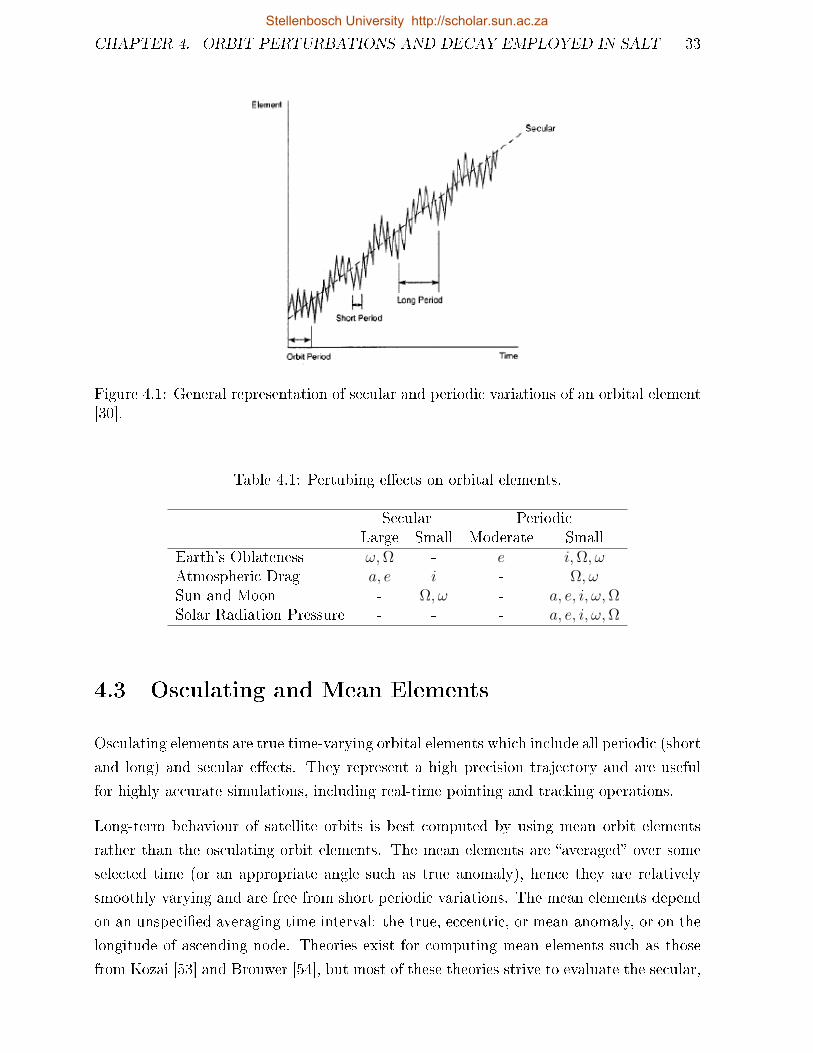
CHAPTER 4. ORBIT PERTURBATIONS AND DECAY EMPLOYED IN SALT 33
Figure 4.1: General representation of secular and periodic variations of an orbital element[30].
Table 4.1: Pertubing eects on orbital elements.
Secular PeriodicLarge Small Moderate Small
Earth's Oblateness ω,Ω - e i,Ω, ωAtmospheric Drag a, e i - Ω, ωSun and Moon - Ω, ω - a, e, i, ω,ΩSolar Radiation Pressure - - - a, e, i, ω,Ω
4.3 Osculating and Mean Elements
Osculating elements are true time-varying orbital elements which include all periodic (short
and long) and secular eects. They represent a high precision trajectory and are useful
for highly accurate simulations, including real-time pointing and tracking operations.
Long-term behaviour of satellite orbits is best computed by using mean orbit elements
rather than the osculating orbit elements. The mean elements are averaged over some
selected time (or an appropriate angle such as true anomaly), hence they are relatively
smoothly varying and are free from short periodic variations. The mean elements depend
on an unspecied averaging time interval: the true, eccentric, or mean anomaly, or on the
longitude of ascending node. Theories exist for computing mean elements such as those
from Kozai [53] and Brouwer [54], but most of these theories strive to evaluate the secular,
Stellenbosch University http://scholar.sun.ac.za
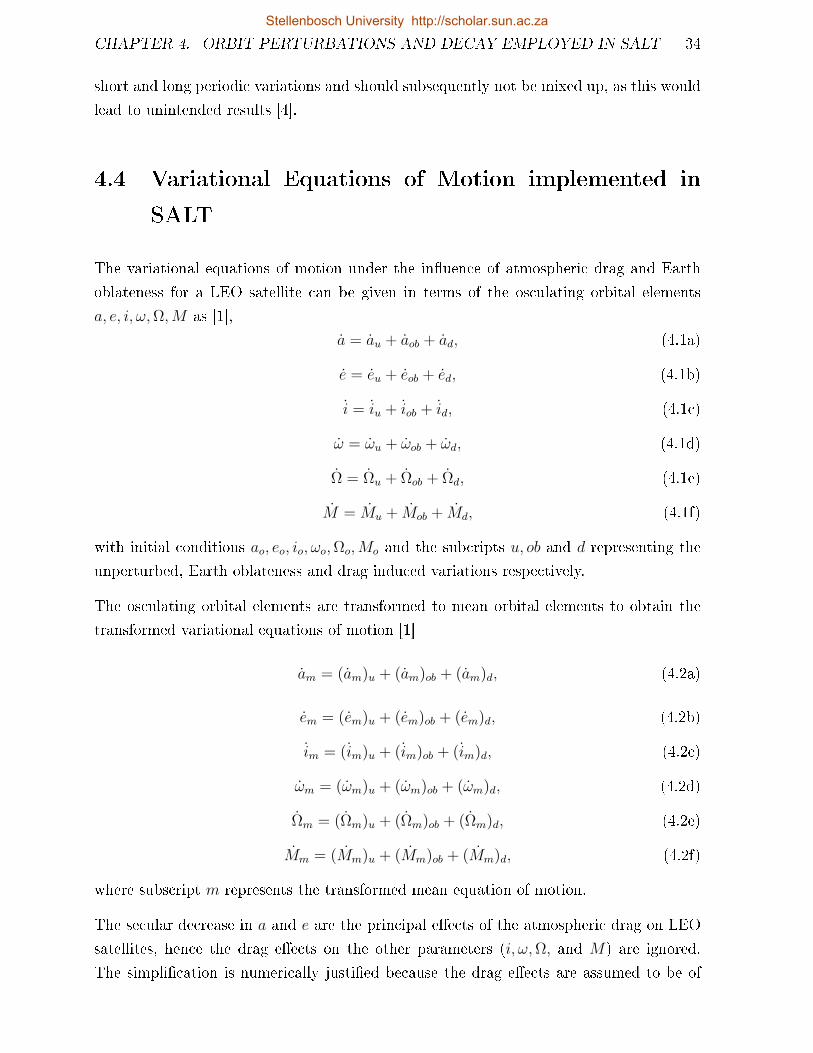
CHAPTER 4. ORBIT PERTURBATIONS AND DECAY EMPLOYED IN SALT 34
short and long periodic variations and should subsequently not be mixed up, as this would
lead to unintended results [4].
4.4 Variational Equations of Motion implemented in
SALT
The variational equations of motion under the inuence of atmospheric drag and Earth
oblateness for a LEO satellite can be given in terms of the osculating orbital elements
a, e, i, ω,Ω,M as [1],
a = au + aob + ad, (4.1a)
e = eu + eob + ed, (4.1b)
i = iu + iob + id, (4.1c)
ω = ωu + ωob + ωd, (4.1d)
Ω = Ωu + Ωob + Ωd, (4.1e)
M = Mu + Mob + Md, (4.1f)
with initial conditions ao, eo, io, ωo,Ωo,Mo and the subcripts u, ob and d representing the
unperturbed, Earth oblateness and drag induced variations respectively.
The osculating orbital elements are transformed to mean orbital elements to obtain the
transformed variational equations of motion [1]
am = (am)u + (am)ob + (am)d, (4.2a)
em = (em)u + (em)ob + (em)d, (4.2b)
im = (im)u + (im)ob + (im)d, (4.2c)
ωm = (ωm)u + (ωm)ob + (ωm)d, (4.2d)
Ωm = (Ωm)u + (Ωm)ob + (Ωm)d, (4.2e)
Mm = (Mm)u + (Mm)ob + (Mm)d, (4.2f)
where subscript m represents the transformed mean equation of motion.
The secular decrease in a and e are the principal eects of the atmospheric drag on LEO
satellites, hence the drag eects on the other parameters (i, ω,Ω, and M) are ignored.
The simplication is numerically justied because the drag eects are assumed to be of
Stellenbosch University http://scholar.sun.ac.za
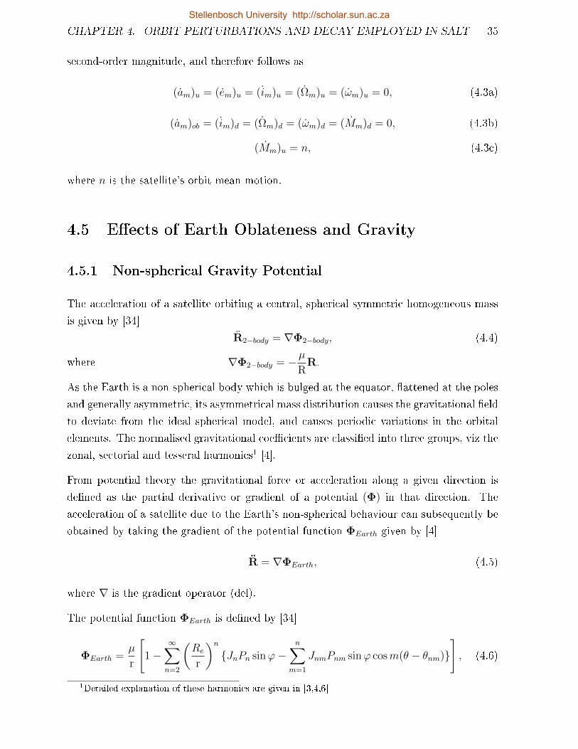
CHAPTER 4. ORBIT PERTURBATIONS AND DECAY EMPLOYED IN SALT 35
second-order magnitude, and therefore follows as
(am)u = (em)u = (im)u = (Ωm)u = (ωm)u = 0, (4.3a)
(am)ob = (im)d = (Ωm)d = (ωm)d = (Mm)d = 0, (4.3b)
(Mm)u = n, (4.3c)
where n is the satellite's orbit mean motion.
4.5 Eects of Earth Oblateness and Gravity
4.5.1 Non-spherical Gravity Potential
The acceleration of a satellite orbiting a central, spherical symmetric homogeneous mass
is given by [34]
R2−body = ∇Φ2−body, (4.4)
where ∇Φ2−body = −µR
R.
As the Earth is a non-spherical body which is bulged at the equator, attened at the poles
and generally asymmetric, its asymmetrical mass distribution causes the gravitational eld
to deviate from the ideal spherical model, and causes periodic variations in the orbital
elements. The normalised gravitational coecients are classied into three groups, viz the
zonal, sectorial and tesseral harmonics1 [4].
From potential theory the gravitational force or acceleration along a given direction is
dened as the partial derivative or gradient of a potential (Φ) in that direction. The
acceleration of a satellite due to the Earth's non-spherical behaviour can subsequently be
obtained by taking the gradient of the potential function ΦEarth given by [4]
R = ∇ΦEarth, (4.5)
where ∇ is the gradient operator (del).
The potential function ΦEarth is dened by [34]
ΦEarth =µ
r
[1−
∞∑n=2
(Re
r
)nJnPn sinϕ−
n∑m=1
JnmPnm sinϕ cosm(θ − θnm)
], (4.6)
1Detailed explanation of these harmonics are given in [3,4,6]
Stellenbosch University http://scholar.sun.ac.za
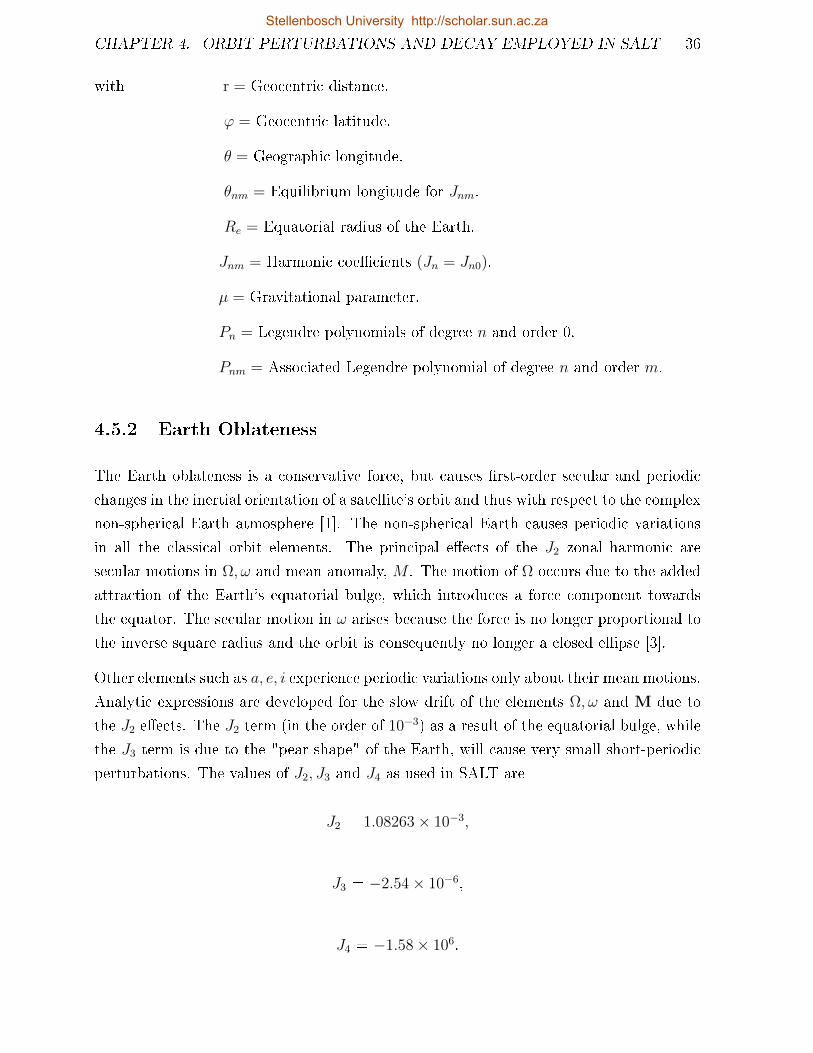
CHAPTER 4. ORBIT PERTURBATIONS AND DECAY EMPLOYED IN SALT 36
with r = Geocentric distance.
ϕ = Geocentric latitude.
θ = Geographic longitude.
θnm = Equilibrium longitude for Jnm.
Re = Equatorial radius of the Earth.
Jnm = Harmonic coecients (Jn = Jn0).
µ = Gravitational parameter.
Pn = Legendre polynomials of degree n and order 0.
Pnm = Associated Legendre polynomial of degree n and order m.
4.5.2 Earth Oblateness
The Earth oblateness is a conservative force, but causes rst-order secular and periodic
changes in the inertial orientation of a satellite's orbit and thus with respect to the complex
non-spherical Earth atmosphere [1]. The non-spherical Earth causes periodic variations
in all the classical orbit elements. The principal eects of the J2 zonal harmonic are
secular motions in Ω, ω and mean anomaly, M . The motion of Ω occurs due to the added
attraction of the Earth's equatorial bulge, which introduces a force component towards
the equator. The secular motion in ω arises because the force is no longer proportional to
the inverse square radius and the orbit is consequently no longer a closed ellipse [3].
Other elements such as a, e, i experience periodic variations only about their mean motions.
Analytic expressions are developed for the slow drift of the elements Ω, ω and M due to
the J2 eects. The J2 term (in the order of 10−3) as a result of the equatorial bulge, while
the J3 term is due to the "pear shape" of the Earth, will cause very small short-periodic
perturbations. The values of J2, J3 and J4 as used in SALT are
J2 = 1.08263× 10⁻³,
J3 = −2.54× 10⁻⁶,
J4 = −1.58× 10⁶.
Stellenbosch University http://scholar.sun.ac.za
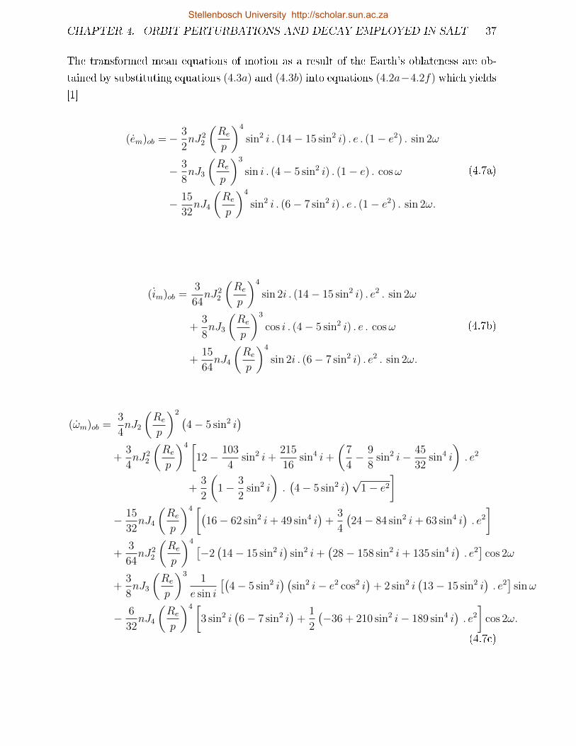
CHAPTER 4. ORBIT PERTURBATIONS AND DECAY EMPLOYED IN SALT 37
The transformed mean equations of motion as a result of the Earth's oblateness are ob-
tained by substituting equations (4.3a) and (4.3b) into equations (4.2a−4.2f) which yields
[1]
(em)ob =− 3
2nJ2
2
(Re
p
)4
sin2 i . (14− 15 sin2 i) . e . (1− e2) . sin 2ω
− 3
8nJ3
(Re
p
)3
sin i . (4− 5 sin2 i) . (1− e) . cosω
− 15
32nJ4
(Re
p
)4
sin2 i . (6− 7 sin2 i) . e . (1− e2) . sin 2ω.
(4.7a)
(im)ob =3
64nJ2
2
(Re
p
)4
sin 2i . (14− 15 sin2 i) . e2 . sin 2ω
+3
8nJ3
(Re
p
)3
cos i . (4− 5 sin2 i) . e . cosω
+15
64nJ4
(Re
p
)4
sin 2i . (6− 7 sin2 i) . e2 . sin 2ω.
(4.7b)
(ωm)ob =3
4nJ2
(Re
p
)2 (4− 5 sin2 i
)+
3
4nJ2
2
(Re
p
)4 [12− 103
4sin2 i+
215
16sin4 i+
(7
4− 9
8sin2 i− 45
32sin4 i
). e2
+3
2
(1− 3
2sin2 i
).(4− 5 sin2 i
)√1− e2
]− 15
32nJ4
(Re
p
)4 [(16− 62 sin2 i+ 49 sin4 i
)+
3
4
(24− 84 sin2 i+ 63 sin4 i
). e2
]+
3
64nJ2
2
(Re
p
)4 [−2(14− 15 sin2 i
)sin2 i+
(28− 158 sin2 i+ 135 sin4 i
). e2]
cos 2ω
+3
8nJ3
(Re
p
)31
e sin i
[(4− 5 sin2 i
) (sin2 i− e2 cos2 i
)+ 2 sin2 i
(13− 15 sin2 i
). e2]
sinω
− 6
32nJ4
(Re
p
)4 [3 sin2 i
(6− 7 sin2 i
)+
1
2
(−36 + 210 sin2 i− 189 sin4 i
). e2
]cos 2ω.
(4.7c)
Stellenbosch University http://scholar.sun.ac.za
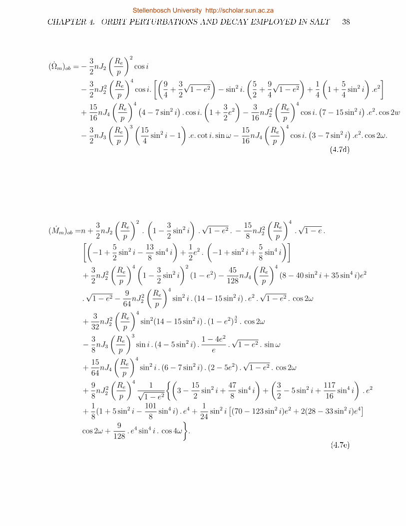
CHAPTER 4. ORBIT PERTURBATIONS AND DECAY EMPLOYED IN SALT 38
(Ωm)ob =− 3
2nJ2
(Re
p
)2
cos i
− 3
2nJ2
2
(Re
p
)4
cos i.
[(9
4+
3
2
√1− e2
)− sin2 i.
(5
2+
9
4
√1− e2
)+
1
4
(1 +
5
4sin2 i
).e2
]+
15
16nJ4
(Re
p
)4 (4− 7 sin2 i
). cos i.
(1 +
3
2e2
)− 3
16nJ2
2
(Re
p
)4
cos i.(7− 15 sin2 i
).e2. cos 2w
− 3
2nJ3
(Re
p
)3(15
4sin2 i− 1
).e. cot i. sinω − 15
16nJ4
(Re
p
)4
cos i.(3− 7 sin2 i
).e2. cos 2ω.
(4.7d)
(Mm)ob =n+3
2nJ2
(Re
p
)2
.
(1− 3
2sin2 i
).√
1− e2 . − 15
8nJ2
2
(Re
p
)4
.√
1− e .[(−1 +
5
2sin2 i− 13
8sin4 i
)+
1
2e2 .
(−1 + sin2 i+
5
8sin4 i
)]+
3
2nJ2
2
(Re
p
)4(1− 3
2sin2 i
)2
(1− e2)− 45
128nJ4
(Re
p
)4
(8− 40 sin2 i+ 35 sin4 i)e2
.√
1− e2 − 9
64nJ2
2
(Re
p
)4
sin2 i . (14− 15 sin2 i) . e2 .√
1− e2 . cos 2ω
+3
32nJ2
2
(Re
p
)4
sin2(14− 15 sin2 i) . (1− e2)32 . cos 2ω
− 3
8nJ3
(Re
p
)3
sin i . (4− 5 sin2 i) .1− 4e2
e.√
1− e2 . sinω
+15
64nJ4
(Re
p
)4
sin2 i . (6− 7 sin2 i) . (2− 5e2) .√
1− e2 . cos 2ω
+9
8nJ2
2
(Re
p
)41√
1− e2
(3− 15
2sin2 i+
47
8sin4 i
)+
(3
2− 5 sin2 i+
117
16sin4 i
). e2
+1
8(1 + 5 sin2 i− 101
8sin4 i) . e4 +
1
24sin2 i
[(70− 123 sin2 i)e2 + 2(28− 33 sin2 i)e4
]cos 2ω +
9
128. e4 sin4 i . cos 4ω
.
(4.7e)
Stellenbosch University http://scholar.sun.ac.za
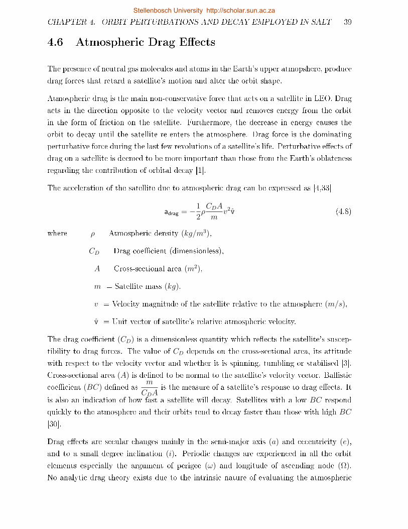
CHAPTER 4. ORBIT PERTURBATIONS AND DECAY EMPLOYED IN SALT 39
4.6 Atmospheric Drag Eects
The presence of neutral gas molecules and atoms in the Earth's upper atmopshere, produce
drag forces that retard a satellite's motion and alter the orbit shape.
Atmospheric drag is the main non-conservative force that acts on a satellite in LEO. Drag
acts in the direction opposite to the velocity vector and removes energy from the orbit
in the form of friction on the satellite. Furthermore, the decrease in energy causes the
orbit to decay until the satellite re-enters the atmosphere. Drag force is the dominating
perturbative force during the last few revolutions of a satellite's life. Perturbative eects of
drag on a satellite is deemed to be more important than those from the Earth's oblateness
regarding the contribution of orbital decay [1].
The acceleration of the satellite due to atmospheric drag can be expressed as [4,33]
adrag = −1
2ρCDA
mv2v (4.8)
where ρ = Atmospheric density (kg/m3),
CD = Drag coecient (dimensionless),
A = Cross-sectional area (m2),
m = Satellite mass (kg),
v = Velocity magnitude of the satellite relative to the atmosphere (m/s),
v = Unit vector of satellite's relative atmospheric velocity.
The drag coecient (CD) is a dimensionless quantity which reects the satellite's suscep-
tibility to drag forces. The value of CD depends on the cross-sectional area, its attitude
with respect to the velocity vector and whether it is spinning, tumbling or stabilised [3].
Cross-sectional area (A) is dened to be normal to the satellite's velocity vector. Ballistic
coecient (BC) dened asm
CDAis the measure of a satellite's response to drag eects. It
is also an indication of how fast a satellite will decay. Satellites with a low BC respond
quickly to the atmosphere and their orbits tend to decay faster than those with high BC
[30].
Drag eects are secular changes mainly in the semi-major axis (a) and eccentricity (e),
and to a small degree inclination (i). Periodic changes are experienced in all the orbit
elements especially the argument of perigee (ω) and longitude of ascending node (Ω).
No analytic drag theory exists due to the intrinsic nature of evaluating the atmospheric
Stellenbosch University http://scholar.sun.ac.za
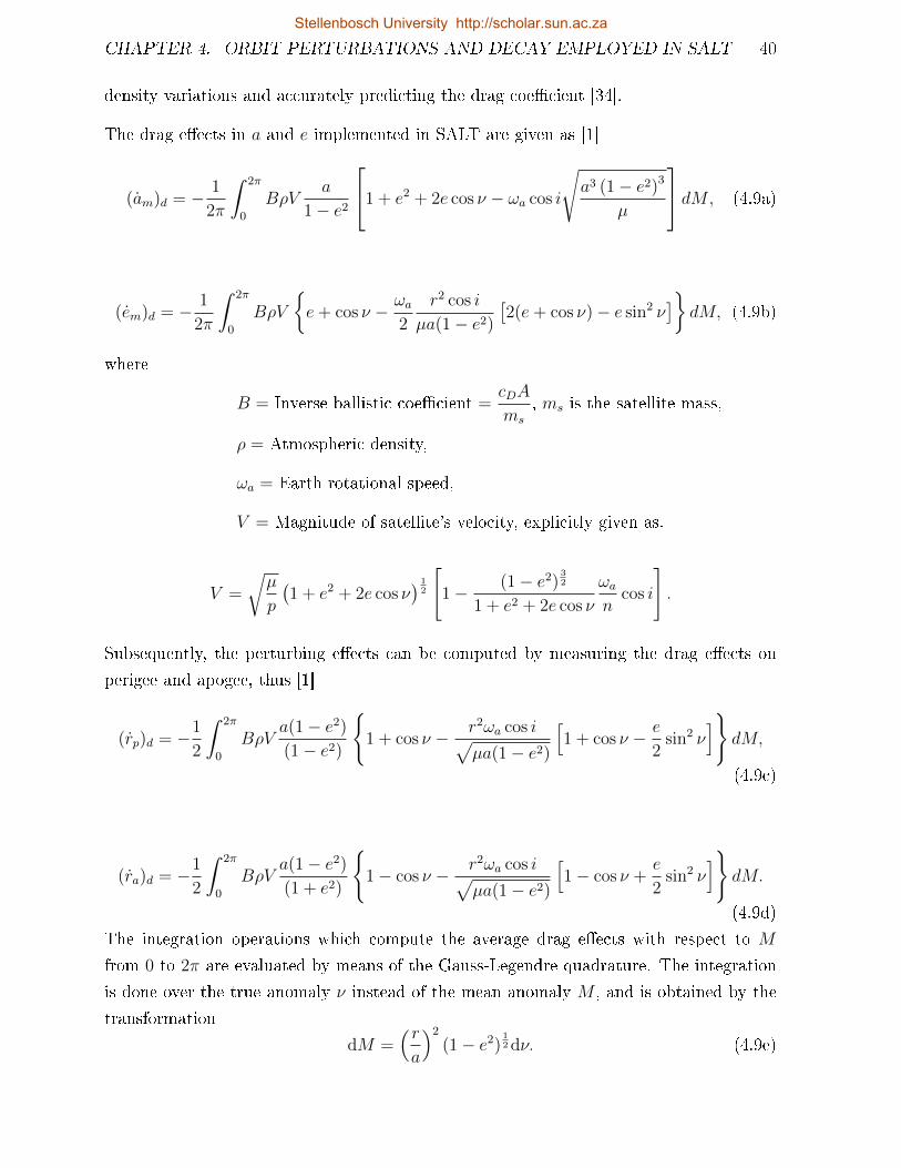
CHAPTER 4. ORBIT PERTURBATIONS AND DECAY EMPLOYED IN SALT 40
density variations and accurately predicting the drag coecient [34].
The drag eects in a and e implemented in SALT are given as [1]
(am)d = − 1
2π
ˆ 2π
0
BρVa
1− e2
1 + e2 + 2e cos ν − ωa cos i
√a3 (1− e2)3
µ
dM, (4.9a)
(em)d = − 1
2π
ˆ 2π
0
BρV
e+ cos ν − ωa
2
r2 cos i
µa(1− e2)
[2(e+ cos ν)− e sin2 ν
]dM, (4.9b)
where
B = Inverse ballistic coecient =cDA
ms
, ms is the satellite mass,
ρ = Atmospheric density,
ωa = Earth rotational speed,
V = Magnitude of satellite's velocity, explicitly given as.
V =
õ
p
(1 + e2 + 2e cos ν
) 12
[1− (1− e2)
32
1 + e2 + 2e cos ν
ωan
cos i
].
Subsequently, the perturbing eects can be computed by measuring the drag eects on
perigee and apogee, thus [1]
(rp)d = −1
2
ˆ 2π
0
BρVa(1− e2)
(1− e2)
1 + cos ν − r2ωa cos i√
µa(1− e2)
[1 + cos ν − e
2sin2 ν
]dM,
(4.9c)
(ra)d = −1
2
ˆ 2π
0
BρVa(1− e2)
(1 + e2)
1− cos ν − r2ωa cos i√
µa(1− e2)
[1− cos ν +
e
2sin2 ν
]dM.
(4.9d)
The integration operations which compute the average drag eects with respect to M
from 0 to 2π are evaluated by means of the Gauss-Legendre quadrature. The integration
is done over the true anomaly ν instead of the mean anomaly M , and is obtained by the
transformation
dM =(ra
)2
(1− e2)12 dν. (4.9e)
Stellenbosch University http://scholar.sun.ac.za
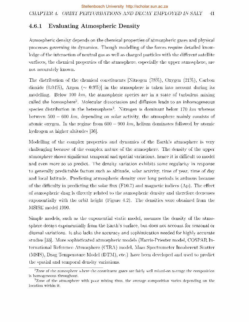
CHAPTER 4. ORBIT PERTURBATIONS AND DECAY EMPLOYED IN SALT 41
4.6.1 Evaluating Atmospheric Density
Atmospheric density depends on the chemical properties of atmospheric gases and physical
processes governing its dynamics. Though modelling of the forces require detailed know-
ledge of the interaction of neutral gas as well as charged particles with the dierent satellite
surfaces, the chemical properties of the atmosphere, especially the upper atmosphere, are
not accurately known.
The distribution of the chemical constituents [Nitrogen (78%), Oxygen (21%), Carbon
dioxide (0.04%), Argon (∼ 0.9%)] in the atmosphere is taken into account during its
modelling. Below 100 km, the atmospheric species are in a state of turbulent mixing
called the homosphere2. Molecular dissociation and diusion leads to an inhomogeneous
species distribution in the heterosphere3. Nitrogen is dominant below 170 km whereas
between 500 − 600 km, depending on solar activity, the atmosphere mainly consists of
atomic oxygen. In the regime from 600 − 900 km, helium dominates followed by atomic
hydrogen at higher altitudes [36].
Modelling of the complex properties and dynamics of the Earth's atmosphere is very
challenging because of the complex nature of the atmosphere. The density of the upper
atmosphere shows signicant temporal and spatial variations, hence it is dicult to model
and even more so to predict. The density variation exhibits some regularity in response
to generally predictable factors such as altitude, solar activity, time of year, time of day
and local latitude. Predicting atmospheric density over long periods is arduous because
of the diculty in predicting the solar ux (F10.7) and magnetic indices (Ap). The eect
of atmospheric drag is directly related to the atmospheric density and therefore decreases
exponentially with the orbit height (Figure 4.2). The densities were obtained from the
MSISE model 1990.
Simple models, such as the exponential static model, assumes the density of the atmo-
sphere decays exponentially from the Earth's surface, but does not account for seasonal or
diurnal variations. It also lacks the accuracy and sophistication needed for highly accurate
studies [33]. More sophisticated atmospheric models (Harris-Priester model, COSPAR In-
ternational Reference Atmosphere (CIRA) model, Mass Spectrometer Incoherent Scatter
(MSIS), Drag Temperature Model (DTM), etc.) have been developed and used to predict
the spatial and temporal density variations.
2Zone of the atmosphere where the constituent gases are fairly well mixed-on average the compositionis homogeneous throughout.
3Zone of the atmosphere with poor mixing thus, the average composition varies depending on thelocation within it.
Stellenbosch University http://scholar.sun.ac.za
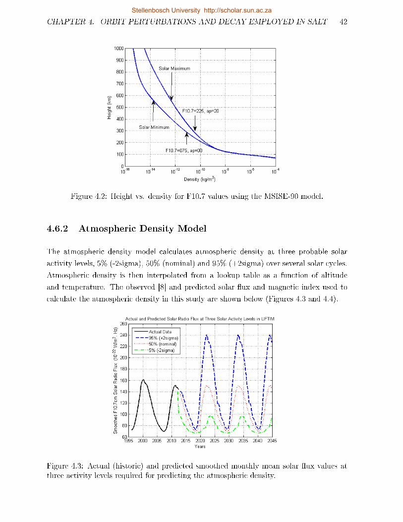
CHAPTER 4. ORBIT PERTURBATIONS AND DECAY EMPLOYED IN SALT 42
Figure 4.2: Height vs. density for F10.7 values using the MSISE-90 model.
4.6.2 Atmospheric Density Model
The atmospheric density model calculates atmospheric density at three probable solar
activity levels, 5% (-2sigma), 50% (nominal) and 95% (+2sigma) over several solar cycles.
Atmospheric density is then interpolated from a lookup table as a function of altitude
and temperature. The observed [8] and predicted solar ux and magnetic index used to
calculate the atmospheric density in this study are shown below (Figures 4.3 and 4.4).
Figure 4.3: Actual (historic) and predicted smoothed monthly mean solar ux values atthree activity levels required for predicting the atmospheric density.
Stellenbosch University http://scholar.sun.ac.za
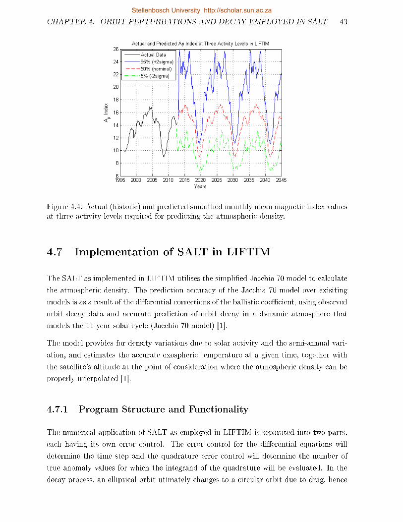
CHAPTER 4. ORBIT PERTURBATIONS AND DECAY EMPLOYED IN SALT 43
Figure 4.4: Actual (historic) and predicted smoothed monthly mean magnetic index valuesat three activity levels required for predicting the atmospheric density.
4.7 Implementation of SALT in LIFTIM
The SALT as implemented in LIFTIM utilises the simplied Jacchia 70 model to calculate
the atmospheric density. The prediction accuracy of the Jacchia 70 model over exisiting
models is as a result of the dierential corrections of the ballistic coecient, using observed
orbit decay data and accurate prediction of orbit decay in a dynamic atmosphere that
models the 11 year solar cycle (Jacchia 70 model) [1].
The model provides for density variations due to solar activity and the semi-annual vari-
ation, and estimates the accurate exospheric temperature at a given time, together with
the satellite's altitude at the point of consideration where the atmospheric density can be
properly interpolated [1].
4.7.1 Program Structure and Functionality
The numerical application of SALT as employed in LIFTIM is separated into two parts,
each having its own error control. The error control for the dierential equations will
determine the time step and the quadrature error control will determine the number of
true anomaly values for which the integrand of the quadrature will be evaluated. In the
decay process, an elliptical orbit utimately changes to a circular orbit due to drag, hence
Stellenbosch University http://scholar.sun.ac.za
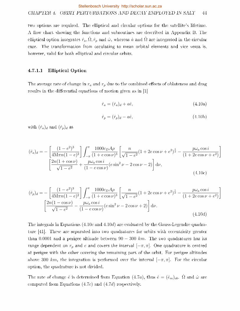
CHAPTER 4. ORBIT PERTURBATIONS AND DECAY EMPLOYED IN SALT 44
two options are required. The elliptical and circular options for the satellite's lifetime.
A ow chart showing the functions and subroutines are described in Appendix B. The
elliptical option integrates ra, Ω, rp and ω, whereas a and Ω are integrated in the circular
case. The transformation from osculating to mean orbital elements and vice versa is,
however, valid for both elliptical and circular orbits.
4.7.1.1 Elliptical Option
The average rate of change in ra and rp due to the combined eects of oblateness and drag
results in the dierential equations of motion given as in [1]
ra = (ra)d + ae, (4.10a)
rp = (rp)d − ae, (4.10b)
with (ra)d and (rp)d as
(ra)d =−[
(1− e2)3
4Mπn(1− e)2
]ˆ π
−π
1000cDAρ
(1 + e cos ν)3
[n√
1− e2(1 + 2e cos ν + e2)
12 − pωa cos i
(1 + 2e cos ν + e2)
][
2n(1 + cos ν)√1− e2
+pωa cos i
(1− e cos ν)(e sin2 ν − 2 cos ν − 2)
]dν,
(4.10c)
(rp)d =−[
(1− e2)3
4Mπn(1− e)2
] ˆ π
−π
1000cDAρ
(1 + e cos ν)3
[n√
1− e2(1 + 2e cos ν + e2)
12 − pωa cos i
(1 + 2e cos ν + e2)
][
2n(1− cos ν)√1− e2
− pωa cos i
(1− e cos ν)(e sin2 ν − 2 cos ν + 2)
]dν.
(4.10d)
The integrals in Equations (4.10c and 4.10d) are evaluated by the Gauss-Legendre quadra-
ture [41]. These are separated into two quadratures for orbits with eccentricity greater
than 0.0001 and a perigee altitude between 90 − 300 km. The two quadratures has its
range dependent on rp and e and covers the interval [−π, π]. One quadrature is centred
at perigee with the other covering the remaining part of the orbit. For perigee altitudes
above 300 km, the integration is performed over the interval [−π, π]. For the circular
option, the quadrature is not divided.
The rate of change e is determined from Equation (4.7a), thus e = (em)ob. Ω and ω are
computed from Equations (4.7c) and (4.7d) respectively.
Stellenbosch University http://scholar.sun.ac.za
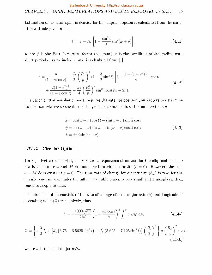
CHAPTER 4. ORBIT PERTURBATIONS AND DECAY EMPLOYED IN SALT 45
Estimation of the atmospheric density for the elliptical option is calculated from the satel-
lite's altitude given as
H = r −Re
[1− sin2 i
fsin2(ω + ν)
], (4.11)
where f is the Earth's atness factor (constant), r is the satellite's orbital radius with
short periodic terms included and is calculated from [1]
r =p
(1 + e cos ν)− J2
2
(Re
p
)2
(1− 3
2sin2 i)
[1 +
1− (1− e2)12
e
]cos ν
+2(1− e2)
12
(1 + e cos ν)+J2
4
(R2e
p
)2
sin2 i cos(2ω + 2ν).
(4.12)
The Jacchia 70 atmospheric model requires the satellite position unit vectors to determine
its position relative to the diurnal bulge. The components of the unit vector are
x = cos(ω + ν) cos Ω− sin(ω + ν) sin Ω cos i,
y = cos(ω + ν) sin Ω + sin(ω + ν) cos Ω cos i,
z = sin i sin(ω + ν).
(4.13)
4.7.1.2 Circular Option
For a perfect circular orbit, the variational equations of motion for the elliptical orbit do
not hold because ω and M are undened for circular orbits (e = 0). However, the sum
ω + M does exists at e = 0. The time rate of change for eccentricity (em) is zero for the
circular case since e, under the inuence of oblateness, is very small and atmospheric drag
tends to keep e at zero.
The circular option consists of the rate of change of semi-major axis (a) and longitude of
ascending node (Ω) respectively, thus
a = −1000√aµ
2M
(1− ωa cos i
n
)2 ˆ π
π
cDAρ dν, (4.14a)
Ω =
−3
2J2 +
[J4
(3.75− 6.5625 sin2 i
)+ J2
2
(5.625− 7.125 sin2 i
)](Re
2
)2n
(Re
a
)2
cos i,
(4.14b)
where a is the semi-major axis.
Stellenbosch University http://scholar.sun.ac.za
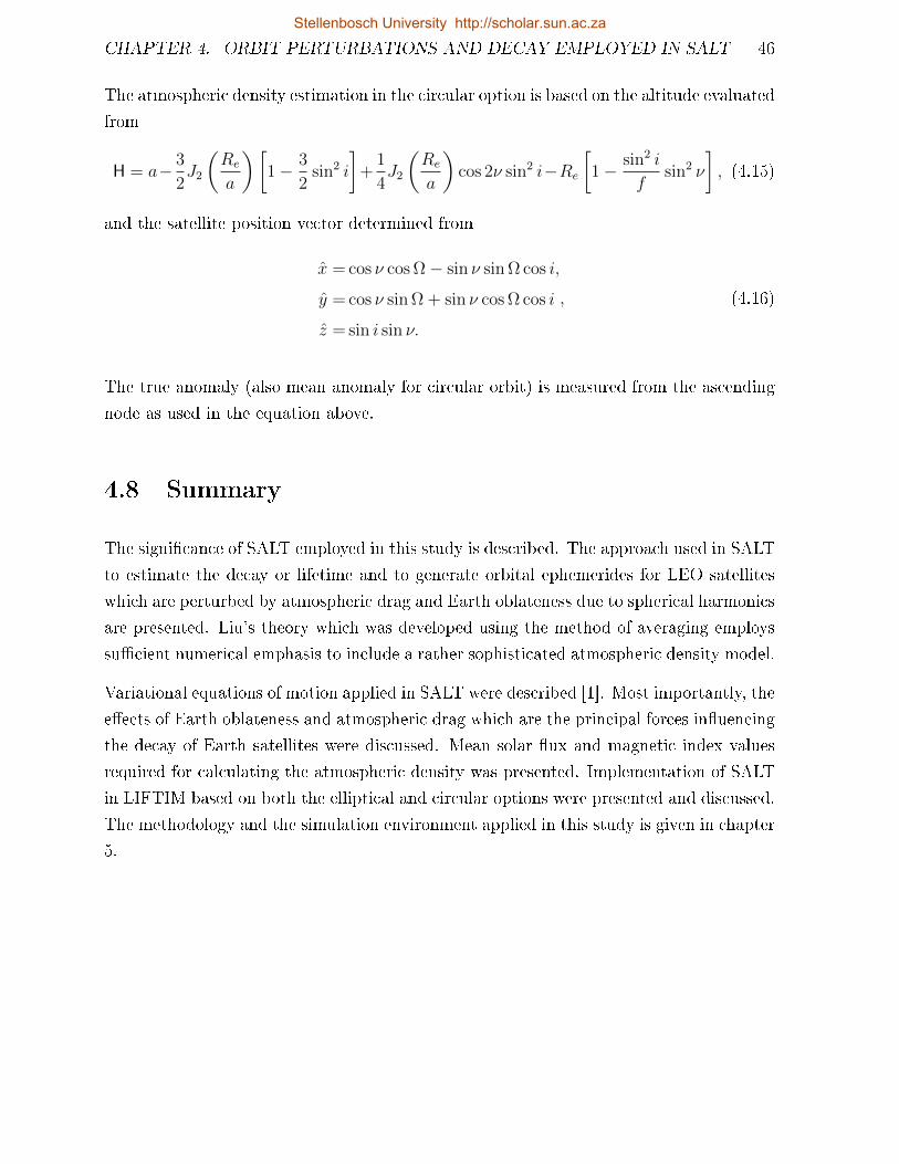
CHAPTER 4. ORBIT PERTURBATIONS AND DECAY EMPLOYED IN SALT 46
The atmospheric density estimation in the circular option is based on the altitude evaluated
from
H = a− 3
2J2
(Re
a
)[1− 3
2sin2 i
]+
1
4J2
(Re
a
)cos 2ν sin2 i−Re
[1− sin2 i
fsin2 ν
], (4.15)
and the satellite position vector determined from
x = cos ν cos Ω− sin ν sin Ω cos i,
y = cos ν sin Ω + sin ν cos Ω cos i
z = sin i sin ν.
, (4.16)
The true anomaly (also mean anomaly for circular orbit) is measured from the ascending
node as used in the equation above.
4.8 Summary
The signicance of SALT employed in this study is described. The approach used in SALT
to estimate the decay or lifetime and to generate orbital ephemerides for LEO satellites
which are perturbed by atmospheric drag and Earth oblateness due to spherical harmonics
are presented. Liu's theory which was developed using the method of averaging employs
sucient numerical emphasis to include a rather sophisticated atmospheric density model.
Variational equations of motion applied in SALT were described [1]. Most importantly, the
eects of Earth oblateness and atmospheric drag which are the principal forces inuencing
the decay of Earth satellites were discussed. Mean solar ux and magnetic index values
required for calculating the atmospheric density was presented. Implementation of SALT
in LIFTIM based on both the elliptical and circular options were presented and discussed.
The methodology and the simulation environment applied in this study is given in chapter
5.
Stellenbosch University http://scholar.sun.ac.za
Chapter 5
Simulation Environment
5.1 Introduction
This chapter describes the methods implemented in this study. The LIFTIM software
package, as explained in Chapter 4, is utilised. The Satellite ToolKit (STK) software was
employed in this study as well. Further analysis on predicting the lifetime of satellites
using solar sails is addressed here. The results of the decay and solar sail predictions will
be presented in Chapter 6.
5.2 LIFTIM Application
LIFTIM [1] was implemented in FORTRAN with MATLAB scripts (Appendix C) written
and executed to achieve the results as presented in this study. LIFTIM was evaluated
against the actual orbit decay histories of Iridium-85 and Starshine-1 satellites prior to
applying the solution to the SUNSAT orbit. LIFTIM was also applied to determine the
expected lifetime of a 1U CubeSAT (ZACUBE-01).
5.3 Data Preparation
The LIFTIM program uses two input les for the lifetime analysis: the solar.dat [8] le
contains observed and long-term predicted solar ux and magnetic activity data, and the
other le contains satellite specic parameters such as initial orbital elements, mass, drag
coecient and model-specic parameters. Input les for the various satellites used in this
47
Stellenbosch University http://scholar.sun.ac.za
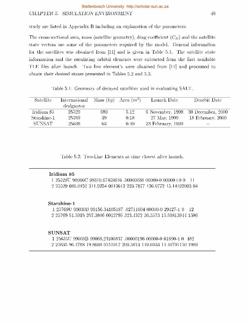
CHAPTER 5. SIMULATION ENVIRONMENT 48
study are listed in Appendix B including an explanation of the parameters.
The cross-sectional area, mass (satellite geometry), drag coecient (CD) and the satellite
state vectors are some of the parameters required by the model. General information
for the satellites was obtained from [11] and is given in Table 5.1. The satellite state
information and the osculating orbital elements were extracted from the rst available
TLE les after launch. Two line element's were obtained from [11] and processed to
obtain their desired states presented in Tables 5.2 and 5.3.
Table 5.1: Geometry of decayed satellites used in evaluating SALT.
Satellite Internationaldesignator
Mass (kg) Area (m2) Launch Date Deorbit Date
Iridium 85 25529 689 5.12 6 November, 1998 30 December, 2000Starshine-1 25769 39 0.18 27 May, 1999 18 February, 2000SUNSAT 25636 63 0.40 23 February, 1999 −
Table 5.2: Two-Line Elements at time closest after launch.
Iridium 851 25529U 98066C 98310.67459616 .00000038 00000-0 00000+0 0 112 25529 086.0152 311.9254 0013613 223.7877 136.0772 15.14192003 04
Starshine-11 25769U 99030B 99156.34105187 .02711664 00000-0 29127-1 0 122 25769 51.5915 257.3806 0012795 323.4372 36.5573 15.59813944 1386
SUNSAT1 25635U 99008B 99068.23100837 .00000196 00000-0 61890-4 0 4822 25635 96.4768 19.8698 0151917 209.5613 149.6933 14.40791150 1989
Stellenbosch University http://scholar.sun.ac.za
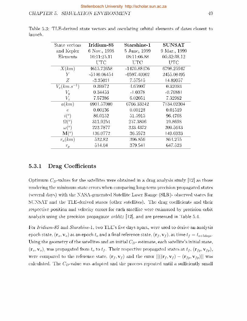
CHAPTER 5. SIMULATION ENVIRONMENT 49
Table 5.3: TLE-derived state vectors and osculating orbital elements of dates closest tolaunch.
State vectorsand KeplerElements
Iridium-856 Nov., 199816:11:25.11
UTC
Starshine-15 June, 199908:11:06.88
UTC
SUNSAT9 Mar., 199905:32:38.12
UTCX(km) 4615.72658 -1470.88476 6798.25947Y -5140.06454 -6597.40002 2455.08495Z -3.25021 7.57515 14.89957
Vx(km.s−1) 0.39972 4.65907 0.32093
Vy 0.34453 -1.0378 -0.76881Vz 7.57386 6.02051 7.32982
a(km) 6901.57000 6766.33242 7134.02304e 0.00136 0.00128 0.01519i(o) 86.0152 51.5915 96.4768Ω(o) 311.9254 257.3806 19.8698ω(o) 223.7877 323.4372 209.5613M(o) 136.0772 36.5573 149.6933ra(km) 532.82 396.856 864.255rp 514.04 379.541 647.523
5.3.1 Drag Coecients
Optimum CD-values for the satellites were obtained in a drag analysis study [12] as those
rendering the minimum state errors when comparing long-term precision propagated states
(several days) with the NASA-generated Satellite Laser Range (SLR)- observed states for
SUNSAT and the TLE-derived states (other satellites). The drag coecients and their
respective position and velocity errors for each satellite were estimated by precision orbit
analysis using the precision propagator orblitz [12], and are presented in Table 5.4.
For Iridium-85 and Starshine-1, two TLE's ve days apart, were used to derive an analysis
epoch state, (ro ,vo) at an epoch to and a nal reference state, (rf ,vf ), at time tf = to+5days.
Using the geometry of the satellites and an initial CD- estimate, each satellite's initial state,
(ro ,vo), was propagated from to to tf . Their respective propagated states at tf , (rfp,vfp),
were compared to the reference state, (rf ,vf ) and the error ||((rf ,vf ) − (rfp,vfp)|| wascalculated. The CD-value was adapted and the process repeated until a suciently small
Stellenbosch University http://scholar.sun.ac.za
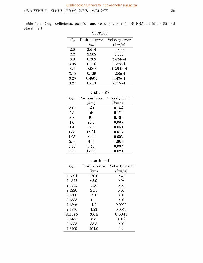
CHAPTER 5. SIMULATION ENVIRONMENT 50
Table 5.4: Drag coecients, position and velocity errors for SUNSAT, Iridium-85 andStarshine-1.
SUNSAT
CD Position error(km)
Velocity error(km/s)
2.0 3.614 0.00382.2 2.965 0.0033.0 0.369 3.834e-43.08 0.116 1.52e-43.1 0.063 1.254e-43.15 0.129 1.96e-43.26 0.4804 5.43e-43.27 0.513 5.77e-4
Iridium-85
CD Position error(km)
Velocity error(km/s)
3.0 150 0.1652.8 164 0.1813.8 91 0.1014.0 76.9 0.0854.4 47.9 0.0504.85 15.31 0.0164.95 8.06 0.0085.0 4.4 0.0045.15 6.45 0.0075.3 17.34 0.020
Starshine-1
CD Position error(km)
Velocity error(km/s)
1.9894 170.0 0.202.0822 65.9 0.082.0955 51.0 0.062.1220 21.1 0.022.1300 12.0 0.012.1353 6.1 0.012.1366 4.7 0.00552.1370 4.22 0.00502.1375 3.64 0.00432.1485 8.8 0.0122.1883 53.8 0.062.3209 204.0 0.2
Stellenbosch University http://scholar.sun.ac.za
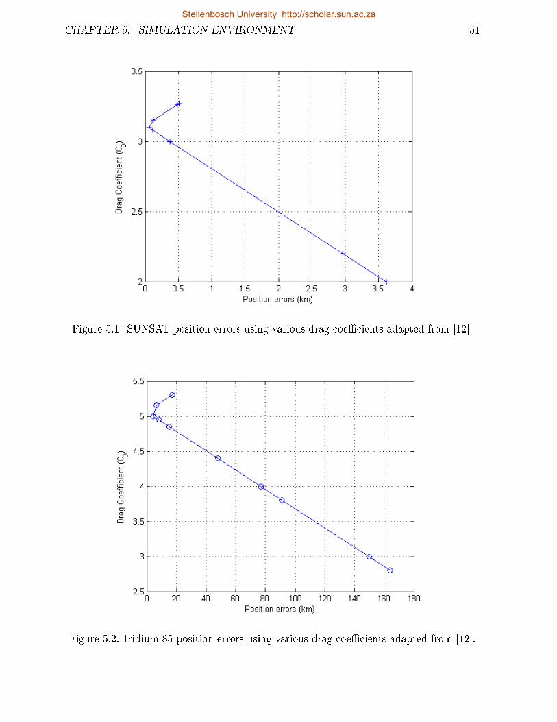
CHAPTER 5. SIMULATION ENVIRONMENT 51
Figure 5.1: SUNSAT position errors using various drag coecients adapted from [12].
Figure 5.2: Iridium-85 position errors using various drag coecients adapted from [12].
Stellenbosch University http://scholar.sun.ac.za
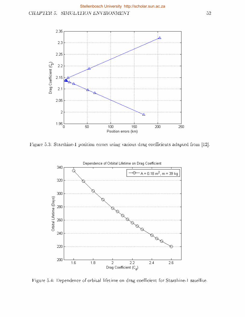
CHAPTER 5. SIMULATION ENVIRONMENT 52
Figure 5.3: Starshine-1 position errors using various drag coecients adapted from [12].
Figure 5.4: Dependence of orbital lifetime on drag coecient for Starshine-1 satellite.
Stellenbosch University http://scholar.sun.ac.za
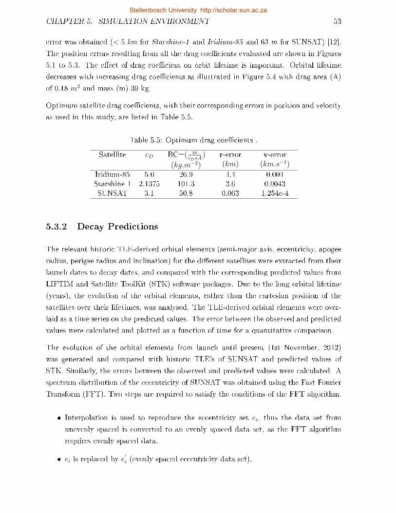
CHAPTER 5. SIMULATION ENVIRONMENT 53
error was obtained (< 5 km for Starshine-1 and Iridium-85 and 63 m for SUNSAT) [12].
The position errors resulting from all the drag coecients evaluated are shown in Figures
5.1 to 5.3. The eect of drag coecient on orbit lifetime is important. Orbital lifetime
decreases with increasing drag coecients as illustrated in Figure 5.4 with drag area (A)
of 0.18 m2 and mass (m) 39 kg.
Optimum satellite drag coecients, with their corresponding errors in position and velocity
as used in this study, are listed in Table 5.5.
Table 5.5: Optimum drag coecients .
Satellite cD BC=( mcD∗A
)
(kg.m−2)
r-error(km)
v-error(km.s−1)
Iridium-85 5.0 26.9 4.4 0.004Starshine-1 2.1375 101.3 3.6 0.0043SUNSAT 3.1 50.8 0.063 1.254e-4
5.3.2 Decay Predictions
The relevant historic TLE-derived orbital elements (semi-major axis, eccentricity, apogee
radius, perigee radius and inclination) for the dierent satellites were extracted from their
launch dates to decay dates, and compared with the corresponding predicted values from
LIFTIM and Satellite ToolKit (STK) software packages. Due to the long orbital lifetime
(years), the evolution of the orbital elements, rather than the cartesian position of the
satellites over their lifetimes, was analysed. The TLE-derived orbital elements were over-
laid as a time series on the predicted values. The error between the observed and predicted
values were calculated and plotted as a function of time for a quantitative comparison.
The evolution of the orbital elements from launch until present (1st November, 2012)
was generated and compared with historic TLE's of SUNSAT and predicted values of
STK. Similarly, the errors between the observed and predicted values were calculated. A
spectrum distribution of the eccentricity of SUNSAT was obtained using the Fast Fourier
Transform (FFT). Two steps are required to satisfy the conditions of the FFT algorithm.
Interpolation is used to reproduce the eccentricity set ei, thus the data set from
unevenly spaced is converted to an evenly spaced data set, as the FFT algorithm
requires evenly spaced data.
ei is replaced by e′i (evenly spaced eccentricity data set).
Stellenbosch University http://scholar.sun.ac.za
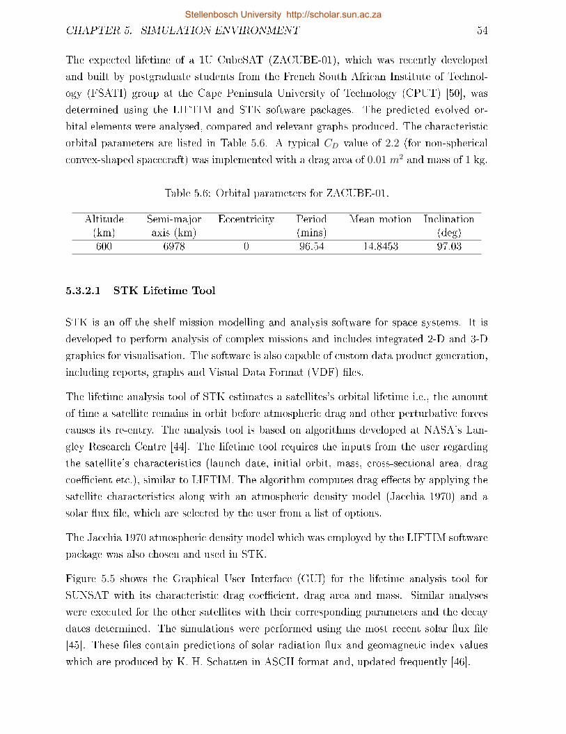
CHAPTER 5. SIMULATION ENVIRONMENT 54
The expected lifetime of a 1U CubeSAT (ZACUBE-01), which was recently developed
and built by postgraduate students from the French South African Institute of Technol-
ogy (FSATI) group at the Cape Peninsula University of Technology (CPUT) [50], was
determined using the LIFTIM and STK software packages. The predicted evolved or-
bital elements were analysed, compared and relevant graphs produced. The characteristic
orbital parameters are listed in Table 5.6. A typical CD value of 2.2 (for non-spherical
convex-shaped spacecraft) was implemented with a drag area of 0.01 m2 and mass of 1 kg.
Table 5.6: Orbital parameters for ZACUBE-01.
Altitude(km)
Semi-majoraxis (km)
Eccentricity Period(mins)
Mean motion Inclination(deg)
600 6978 0 96.54 14.8453 97.03
5.3.2.1 STK Lifetime Tool
STK is an o-the-shelf mission modelling and analysis software for space systems. It is
developed to perform analysis of complex missions and includes integrated 2-D and 3-D
graphics for visualisation. The software is also capable of custom data product generation,
including reports, graphs and Visual Data Format (VDF) les.
The lifetime analysis tool of STK estimates a satellites's orbital lifetime i.e., the amount
of time a satellite remains in orbit before atmospheric drag and other perturbative forces
causes its re-entry. The analysis tool is based on algorithms developed at NASA's Lan-
gley Research Centre [44]. The lifetime tool requires the inputs from the user regarding
the satellite's characteristics (launch date, initial orbit, mass, cross-sectional area, drag
coecient etc.), similar to LIFTIM. The algorithm computes drag eects by applying the
satellite characteristics along with an atmospheric density model (Jacchia 1970) and a
solar ux le, which are selected by the user from a list of options.
The Jacchia 1970 atmospheric density model which was employed by the LIFTIM software
package was also chosen and used in STK.
Figure 5.5 shows the Graphical User Interface (GUI) for the lifetime analysis tool for
SUNSAT with its characteristic drag coecient, drag area and mass. Similar analyses
were executed for the other satellites with their corresponding parameters and the decay
dates determined. The simulations were performed using the most recent solar ux le
[45]. These les contain predictions of solar radiation ux and geomagnetic index values
which are produced by K. H. Schatten in ASCII format and, updated frequently [46].
Stellenbosch University http://scholar.sun.ac.za
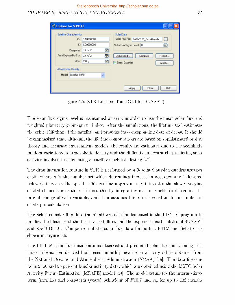
CHAPTER 5. SIMULATION ENVIRONMENT 55
Figure 5.5: STK Lifetime Tool (GUI for SUNSAT).
The solar ux sigma level is maintained at zero, in order to use the mean solar ux and
weighted planetary geomagnetic index. After the simulations, the lifetime tool estimates
the orbital lifetime of the satellite and provides its corresponding date of decay. It should
be emphasised that, although the lifetime computations are based on sophisticated orbital
theory and accurate environment models, the results are estimates due to the seemingly
random variations in atmospheric density and the diculty in accurately predicting solar
activity involved in calculating a satellite's orbital lifetime [47].
The drag integration routine in STK is performed by n 9-point Gaussian quadratures per
orbit, where n is the number set which determines increase in accuracy and if lowered
below 6, increases the speed. This routine approximately integrates the slowly varying
orbital elements over time. It does this by integrating over one orbit to determine the
rate-of-change of each variable, and then assumes this rate is constant for n number of
orbits per calculation
The Schatten solar ux data (nominal) was also implemented in the LIFTIM program to
predict the lifetimes of the test case satellites and the expected deorbit dates of SUNSAT
and ZACUBE-01. Comparison of the solar ux data for both LIFTIM and Schatten is
shown in Figure 5.6.
The LIFTIM solar ux data contains observed and predicted solar ux and geomagnetic
index information, derived from recent monthly mean solar activity values obtained from
the National Oceanic and Atmospheric Administration (NOAA) [48]. The data le con-
tains 5, 50 and 95 percentile solar activity data, which are obtained using the MSFC Solar
Activity Future Estimation (MSAFE) model [49]. The model estimates the intermediate-
term (months) and long-term (years) behaviour of F10.7 and Ap for up to 132 months
Stellenbosch University http://scholar.sun.ac.za
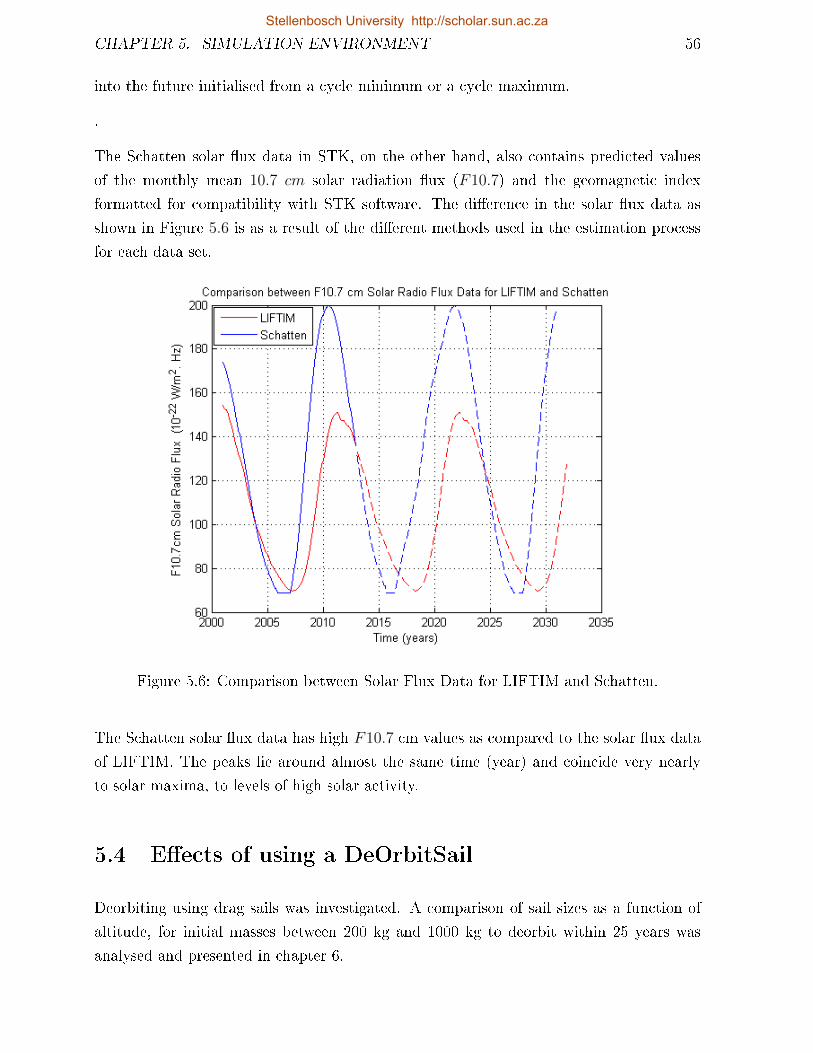
CHAPTER 5. SIMULATION ENVIRONMENT 56
into the future initialised from a cycle minimum or a cycle maximum.
.
The Schatten solar ux data in STK, on the other hand, also contains predicted values
of the monthly mean 10.7 cm solar radiation ux (F10.7) and the geomagnetic index
formatted for compatibility with STK software. The dierence in the solar ux data as
shown in Figure 5.6 is as a result of the dierent methods used in the estimation process
for each data set.
Figure 5.6: Comparison between Solar Flux Data for LIFTIM and Schatten.
The Schatten solar ux data has high F10.7 cm values as compared to the solar ux data
of LIFTIM. The peaks lie around almost the same time (year) and coincide very nearly
to solar maxima, to levels of high solar activity.
5.4 Eects of using a DeOrbitSail
Deorbiting using drag sails was investigated. A comparison of sail sizes as a function of
altitude, for initial masses between 200 kg and 1000 kg to deorbit within 25 years was
analysed and presented in chapter 6.
Stellenbosch University http://scholar.sun.ac.za
CHAPTER 5. SIMULATION ENVIRONMENT 57
The lifetime of SUNSAT was predicted assuming a 10 m2 sail deployed. Similarly, the 1U
CubeSat (ZACUBE-01) lifetime was also estimated assuming 10 m2 drag sail. Compar-
isons were made and the advantage of a low-cost solar sail was established.
The drag sail concept was also applied to Iridium-85 and Starshine-1 satellites to inves-
tigate decreased lifetimes should a sail have been used. Relevant graphs are presented in
Chapter 6.
5.5 Summary
This chapter presented the approach used in this study. Application of the lifetime software
packages (LIFTIM and STK) were discussed. Drag coecients were presented with their
respective position and velocity errors as estimated by precision orbit analysis using the
precision propagator orblitz. Evaluation and methods used in the decay prediction of
the test case satellites, SUNSAT and 1U CubeSAT (ZACUBE-01) were described. The
method used in deorbiting satellites employing solar sails was addressed briey and will
be presented and discussed in Chapter 6.
Stellenbosch University http://scholar.sun.ac.za
Chapter 6
Results and Discussion
6.1 Introduction
This chapter presents a comparison of historic (observed) TLE-derived orbital elements
and those predicted by the decay and lifetime packages LIFTIM and STK for all the satel-
lites considered in this study. The test results are presented for two considered scenarios:
observed decay histories and, the predicted decay results when employing a drag sail to
demonstrate the deorbitsail concept as space debris mitigation mechanism.
6.2 Schatten data adopted in LIFTIM
A comparative investigation was performed using the Schatten solar ux data (nominal)
[45] in the LIFTIM program (LIFTIMSchatten) to determine variations in the evolved orbital
parameters (semi-major axis, eccentricity, inclination, apogee height) for the test case
satellites, SUNSAT and ZACUBE-01. The characteristic orbital parameters, mass and
CD values for the dierent satellites were maintained. Predicted orbit decay dates for the
respective satellites were estimated.
58
Stellenbosch University http://scholar.sun.ac.za
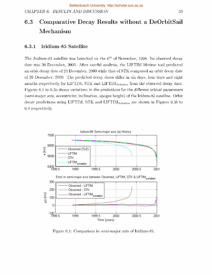
CHAPTER 6. RESULTS AND DISCUSSION 59
6.3 Comparative Decay Results without a DeOrbitSail
Mechanism
6.3.1 Iridium-85 Satellite
The Iridium-85 satellite was launched on the 6th of November, 1998. Its observed decay
date was 30 December, 2000. After careful analysis, the LIFTIM lifetime tool predicted
an orbit decay date of 24 December, 2000 while that of STK computed an orbit decay date
of 26 December, 2000. The predicted decay dates dier in six days, four days and eight
months respectively for LIFTIM, STK and LIFTIMSchatten from the observed decay date.
Figures 6.1 to 6.3a shows variations in the predictions for the dierent orbital parameters
(semi-major axis, eccentricity, inclination, apogee height) of the Iridum-85 satellite. Orbit
decay predictions using LIFTIM, STK and LIFTIMSchatten are shown in Figures 6.3b to
6.4 respectively.
Figure 6.1: Comparison in semi-major axis of Iridium-85.
Stellenbosch University http://scholar.sun.ac.za
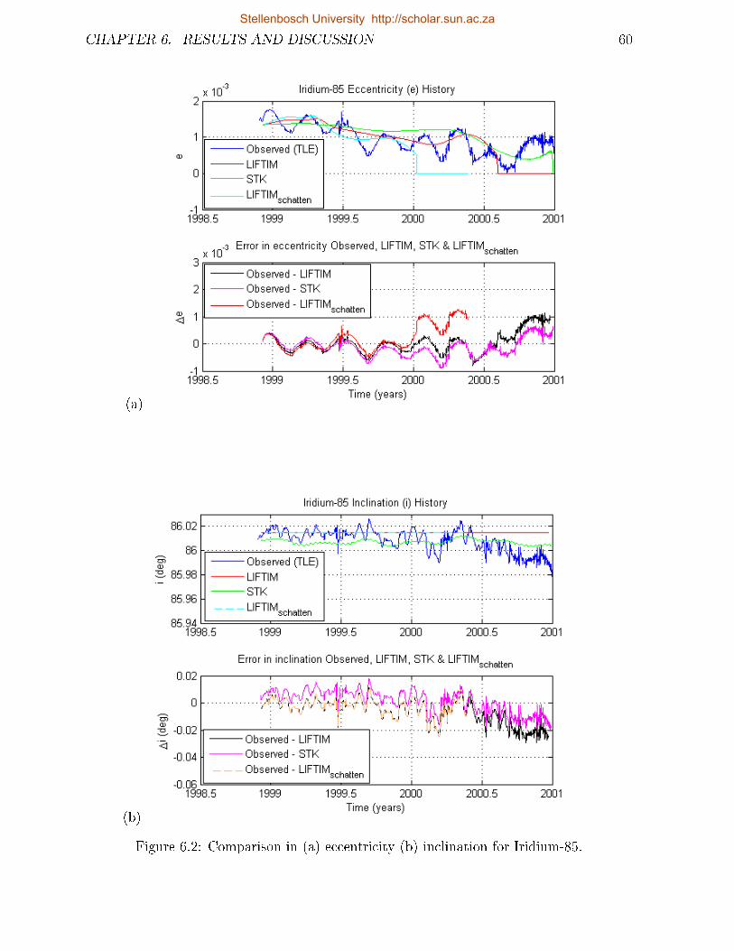
CHAPTER 6. RESULTS AND DISCUSSION 60
(a)
(b)
Figure 6.2: Comparison in (a) eccentricity (b) inclination for Iridium-85.
Stellenbosch University http://scholar.sun.ac.za
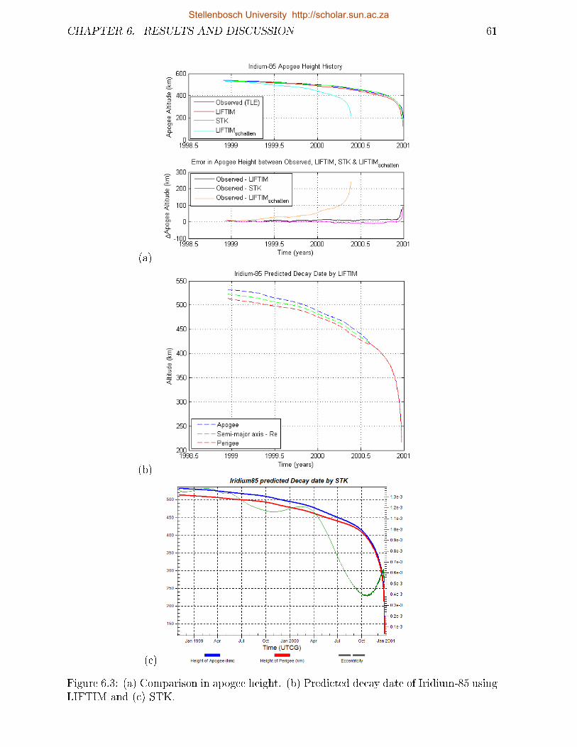
CHAPTER 6. RESULTS AND DISCUSSION 61
(a)
(b)
(c)
Figure 6.3: (a) Comparison in apogee height. (b) Predicted decay date of Iridium-85 usingLIFTIM and (c) STK.
Stellenbosch University http://scholar.sun.ac.za
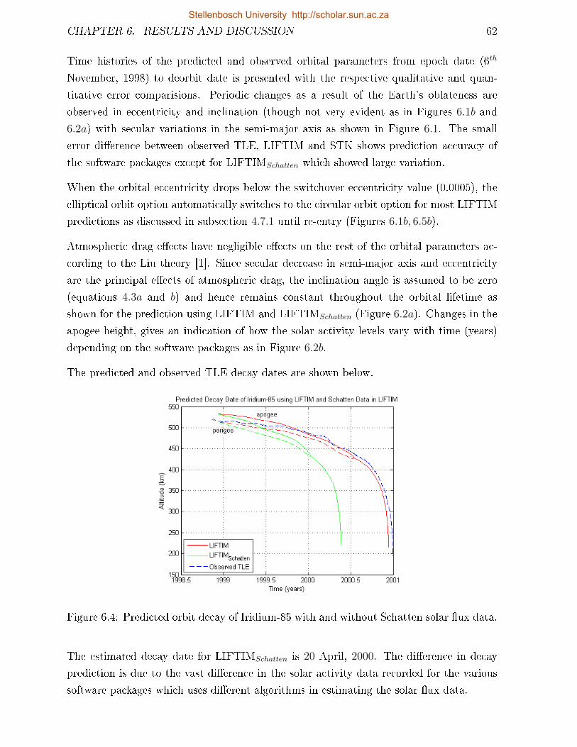
CHAPTER 6. RESULTS AND DISCUSSION 62
Time histories of the predicted and observed orbital parameters from epoch date (6th
November, 1998) to deorbit date is presented with the respective qualitative and quan-
titative error comparisions. Periodic changes as a result of the Earth's oblateness are
observed in eccentricity and inclination (though not very evident as in Figures 6.1b and
6.2a) with secular variations in the semi-major axis as shown in Figure 6.1. The small
error dierence between observed TLE, LIFTIM and STK shows prediction accuracy of
the software packages except for LIFTIMSchatten which showed large variation.
When the orbital eccentricity drops below the switchover eccentricity value (0.0005), the
elliptical orbit option automatically switches to the circular orbit option for most LIFTIM
predictions as discussed in subsection 4.7.1 until re-entry (Figures 6.1b, 6.5b).
Atmospheric drag eects have negligible eects on the rest of the orbital parameters ac-
cording to the Liu theory [1]. Since secular decrease in semi-major axis and eccentricity
are the principal eects of atmospheric drag, the inclination angle is assumed to be zero
(equations 4.3a and b) and hence remains constant throughout the orbital lifetime as
shown for the prediction using LIFTIM and LIFTIMSchatten (Figure 6.2a). Changes in the
apogee height, gives an indication of how the solar activity levels vary with time (years)
depending on the software packages as in Figure 6.2b.
The predicted and observed TLE decay dates are shown below.
Figure 6.4: Predicted orbit decay of Iridium-85 with and without Schatten solar ux data.
The estimated decay date for LIFTIMSchatten is 20 April, 2000. The dierence in decay
prediction is due to the vast dierence in the solar activity data recorded for the various
software packages which uses dierent algorithms in estimating the solar ux data.
Stellenbosch University http://scholar.sun.ac.za
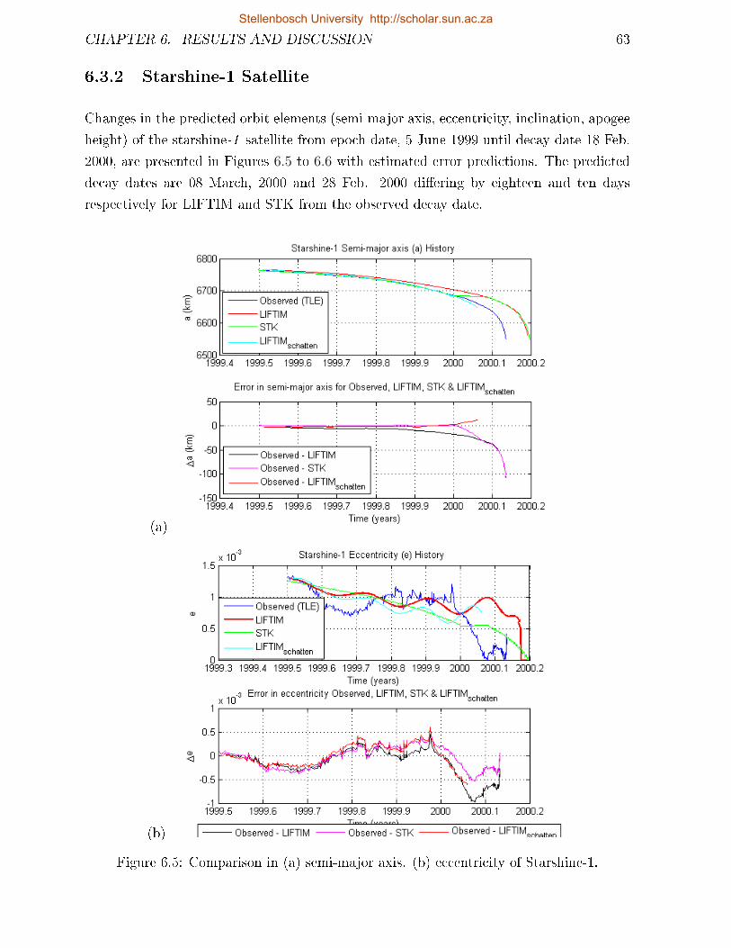
CHAPTER 6. RESULTS AND DISCUSSION 63
6.3.2 Starshine-1 Satellite
Changes in the predicted orbit elements (semi-major axis, eccentricity, inclination, apogee
height) of the starshine-1 satellite from epoch date, 5 June 1999 until decay date 18 Feb.
2000, are presented in Figures 6.5 to 6.6 with estimated error predictions. The predicted
decay dates are 08 March, 2000 and 28 Feb. 2000 diering by eighteen and ten days
respectively for LIFTIM and STK from the observed decay date.
(a)
(b)
Figure 6.5: Comparison in (a) semi-major axis. (b) eccentricity of Starshine-1.
Stellenbosch University http://scholar.sun.ac.za
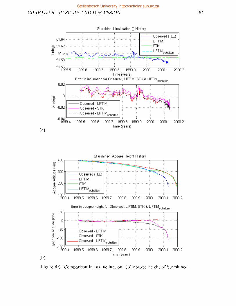
CHAPTER 6. RESULTS AND DISCUSSION 64
(a)
(b)
Figure 6.6: Comparison in (a) inclination. (b) apogee height of Starshine-1.
Stellenbosch University http://scholar.sun.ac.za
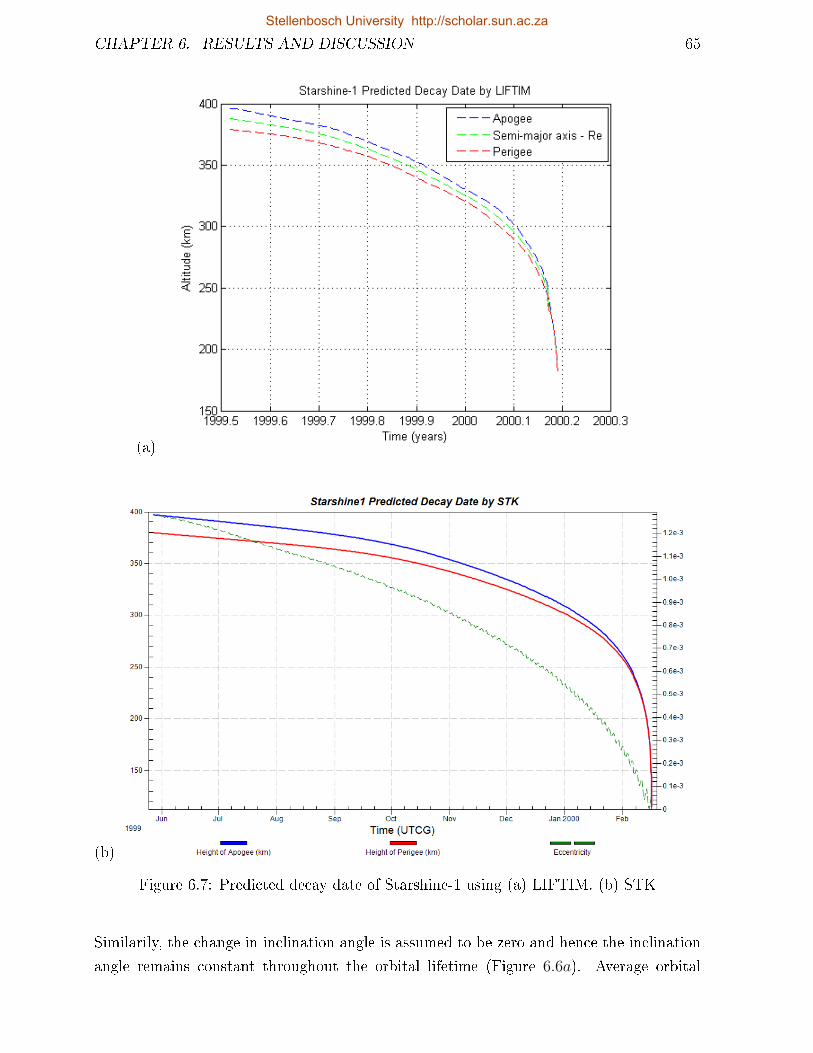
CHAPTER 6. RESULTS AND DISCUSSION 65
(a)
(b)
Figure 6.7: Predicted decay date of Starshine-1 using (a) LIFTIM. (b) STK
Similarily, the change in inclination angle is assumed to be zero and hence the inclination
angle remains constant throughout the orbital lifetime (Figure 6.6a). Average orbital
Stellenbosch University http://scholar.sun.ac.za
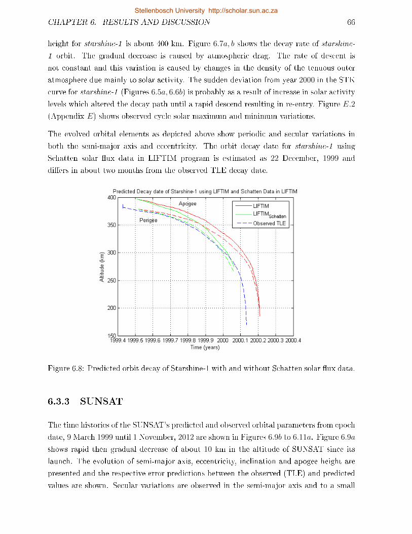
CHAPTER 6. RESULTS AND DISCUSSION 66
height for starshine-1 is about 400 km. Figure 6.7a, b shows the decay rate of starshine-
1 orbit. The gradual decrease is caused by atmospheric drag. The rate of descent is
not constant and this variation is caused by changes in the density of the tenuous outer
atmosphere due mainly to solar activity. The sudden deviation from year 2000 in the STK
curve for starshine-1 (Figures 6.5a, 6.6b) is probably as a result of increase in solar activity
levels which altered the decay path until a rapid descend resulting in re-entry. Figure E.2
(Appendix E) shows observed cycle solar maximum and minimum variations.
The evolved orbital elements as depicted above show periodic and secular variations in
both the semi-major axis and eccentricity. The orbit decay date for starshine-1 using
Schatten solar ux data in LIFTIM program is estimated as 22 December, 1999 and
diers in about two months from the observed TLE decay date.
Figure 6.8: Predicted orbit decay of Starshine-1 with and without Schatten solar ux data.
6.3.3 SUNSAT
The time histories of the SUNSAT's predicted and observed orbital parameters from epoch
date, 9 March 1999 until 1 November, 2012 are shown in Figures 6.9b to 6.11a. Figure 6.9a
shows rapid then gradual decrease of about 10 km in the altitude of SUNSAT since its
launch. The evolution of semi-major axis, eccentricity, inclination and apogee height are
presented and the respective error predictions between the observed (TLE) and predicted
values are shown. Secular variations are observed in the semi-major axis and to a small
Stellenbosch University http://scholar.sun.ac.za
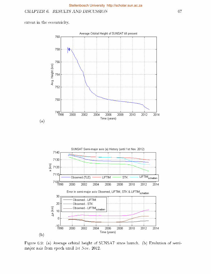
CHAPTER 6. RESULTS AND DISCUSSION 67
extent in the eccentricity.
(a)
(b)
Figure 6.9: (a) Average orbital height of SUNSAT since launch. (b) Evolution of semi-major axis from epoch until 1st Nov. 2012.
Stellenbosch University http://scholar.sun.ac.za
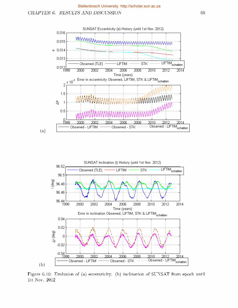
CHAPTER 6. RESULTS AND DISCUSSION 68
(a)
(b)
Figure 6.10: Evolution of (a) eccentricity. (b) inclination of SUNSAT from epoch until1st Nov. 2012
Stellenbosch University http://scholar.sun.ac.za
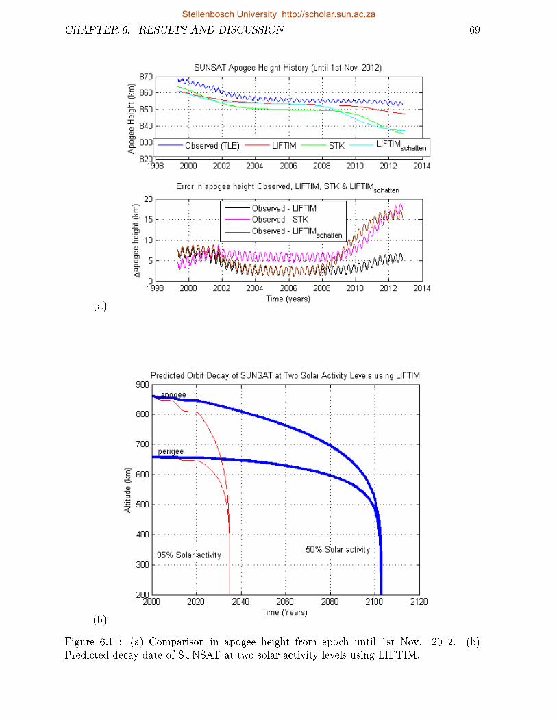
CHAPTER 6. RESULTS AND DISCUSSION 69
(a)
(b)
Figure 6.11: (a) Comparison in apogee height from epoch until 1st Nov. 2012. (b)Predicted decay date of SUNSAT at two solar activity levels using LIFTIM.
Stellenbosch University http://scholar.sun.ac.za
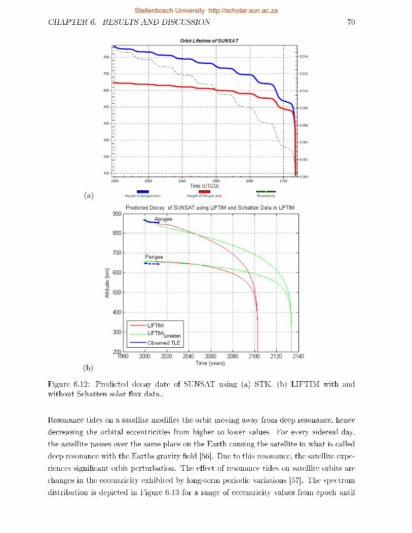
CHAPTER 6. RESULTS AND DISCUSSION 70
(a)
(b)
Figure 6.12: Predicted decay date of SUNSAT using (a) STK. (b) LIFTIM with andwithout Schatten solar ux data..
Resonance tides on a satellite modies the orbit moving away from deep resonance, hence
decreasing the orbital eccentricities from higher to lower values. For every sidereal day,
the satellite passes over the same place on the Earth causing the satellite in what is called
deep resonance with the Earths gravity eld [56]. Due to this resonance, the satellite expe-
riences signicant orbit perturbation. The eect of resonance tides on satellite orbits are
changes in the eccentricity exhibited by long-term periodic variations [57]. The spectrum
distribution is depicted in Figure 6.13 for a range of eccentricity values from epoch until
Stellenbosch University http://scholar.sun.ac.za
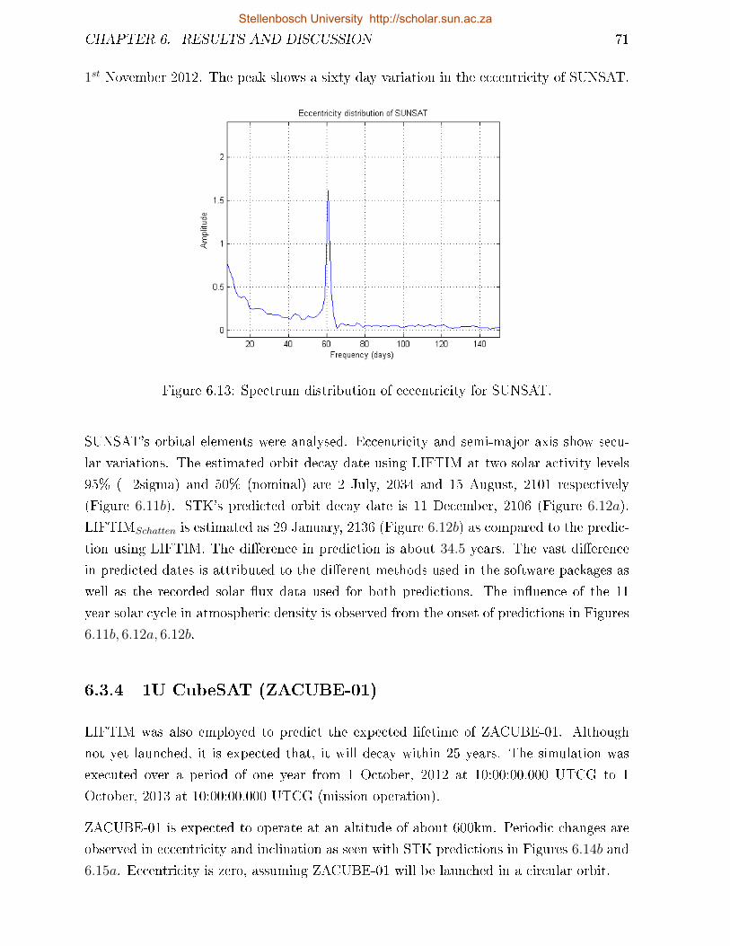
CHAPTER 6. RESULTS AND DISCUSSION 71
1st November 2012. The peak shows a sixty day variation in the eccentricity of SUNSAT.
Figure 6.13: Spectrum distribution of eccentricity for SUNSAT.
SUNSAT's orbital elements were analysed. Eccentricity and semi-major axis show secu-
lar variations. The estimated orbit decay date using LIFTIM at two solar activity levels
95% (+2sigma) and 50% (nominal) are 2 July, 2034 and 15 August, 2101 respectively
(Figure 6.11b). STK's predicted orbit decay date is 11 December, 2106 (Figure 6.12a).
LIFTIMSchatten is estimated as 29 January, 2136 (Figure 6.12b) as compared to the predic-
tion using LIFTIM. The dierence in prediction is about 34.5 years. The vast dierence
in predicted dates is attributed to the dierent methods used in the software packages as
well as the recorded solar ux data used for both predictions. The inuence of the 11
year solar cycle in atmospheric density is observed from the onset of predictions in Figures
6.11b, 6.12a, 6.12b.
6.3.4 1U CubeSAT (ZACUBE-01)
LIFTIM was also employed to predict the expected lifetime of ZACUBE-01. Although
not yet launched, it is expected that, it will decay within 25 years. The simulation was
executed over a period of one year from 1 October, 2012 at 10:00:00.000 UTCG to 1
October, 2013 at 10:00:00.000 UTCG (mission operation).
ZACUBE-01 is expected to operate at an altitude of about 600km. Periodic changes are
observed in eccentricity and inclination as seen with STK predictions in Figures 6.14b and
6.15a. Eccentricity is zero, assuming ZACUBE-01 will be launched in a circular orbit.
Stellenbosch University http://scholar.sun.ac.za
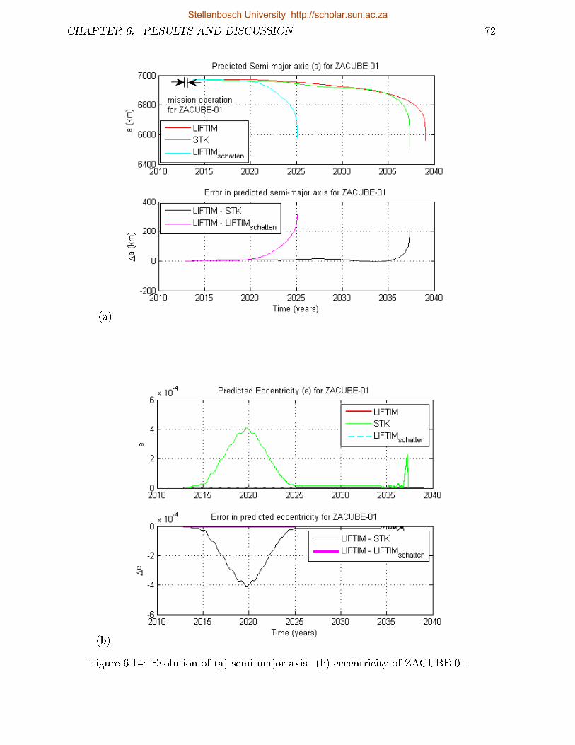
CHAPTER 6. RESULTS AND DISCUSSION 72
(a)
(b)
Figure 6.14: Evolution of (a) semi-major axis. (b) eccentricity of ZACUBE-01.
Stellenbosch University http://scholar.sun.ac.za
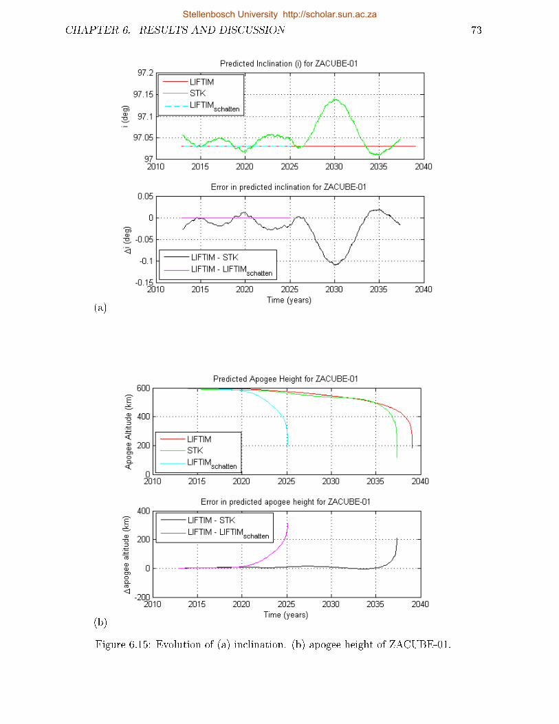
CHAPTER 6. RESULTS AND DISCUSSION 73
(a)
(b)
Figure 6.15: Evolution of (a) inclination. (b) apogee height of ZACUBE-01.
Stellenbosch University http://scholar.sun.ac.za
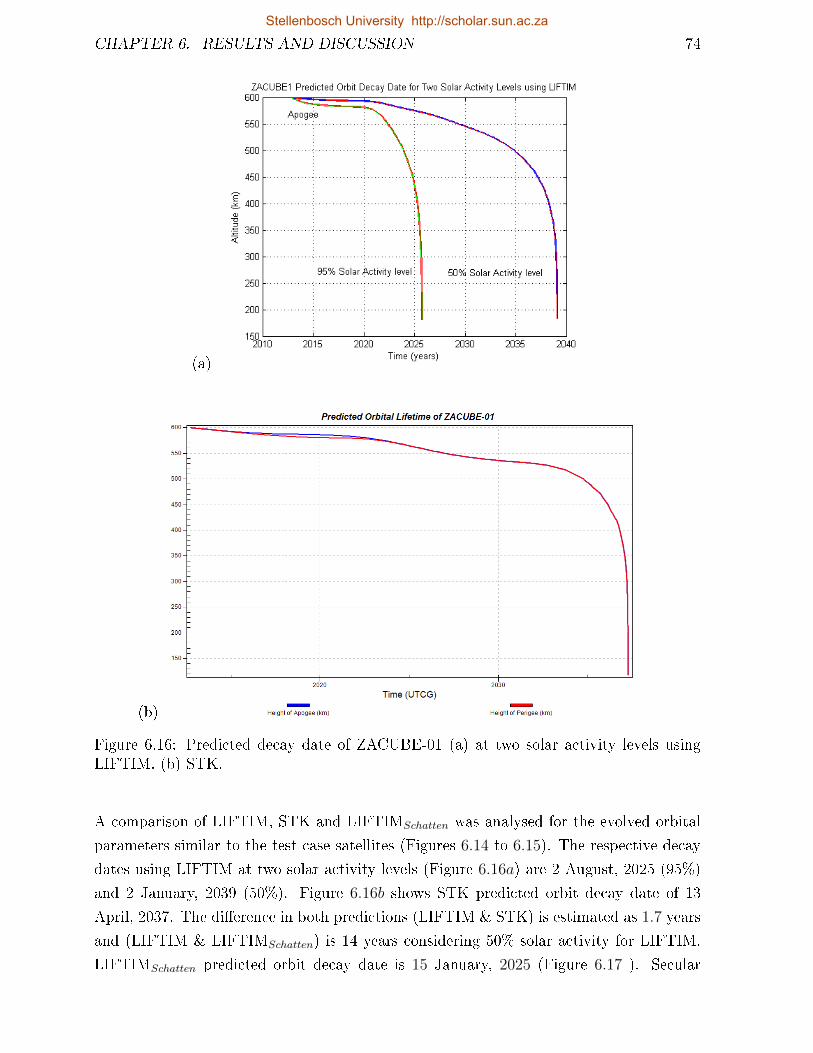
CHAPTER 6. RESULTS AND DISCUSSION 74
(a)
(b)
Figure 6.16: Predicted decay date of ZACUBE-01 (a) at two solar activity levels usingLIFTIM. (b) STK.
A comparison of LIFTIM, STK and LIFTIMSchatten was analysed for the evolved orbital
parameters similar to the test case satellites (Figures 6.14 to 6.15). The respective decay
dates using LIFTIM at two solar activity levels (Figure 6.16a) are 2 August, 2025 (95%)
and 2 January, 2039 (50%). Figure 6.16b shows STK predicted orbit decay date of 13
April, 2037. The dierence in both predictions (LIFTIM & STK) is estimated as 1.7 years
and (LIFTIM & LIFTIMSchatten) is 14 years considering 50% solar activity for LIFTIM.
LIFTIMSchatten predicted orbit decay date is 15 January, 2025 (Figure 6.17 ). Secular
Stellenbosch University http://scholar.sun.ac.za
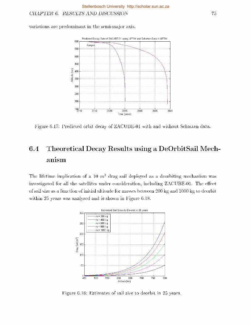
CHAPTER 6. RESULTS AND DISCUSSION 75
variations are predominant in the semi-major axis.
Figure 6.17: Predicted orbit decay of ZACUBE-01 with and without Schatten data.
6.4 Theoretical Decay Results using a DeOrbitSail Mech-
anism
The lifetime implication of a 10 m2 drag sail deployed as a deorbiting mechanism was
investigated for all the satellites under consideration, including ZACUBE-01. The eect
of sail size as a function of initial altitude for masses between 200 kg and 1000 kg to deorbit
within 25 years was analysed and is shown in Figure 6.18.
Figure 6.18: Estimates of sail size to deorbit in 25 years.
Stellenbosch University http://scholar.sun.ac.za
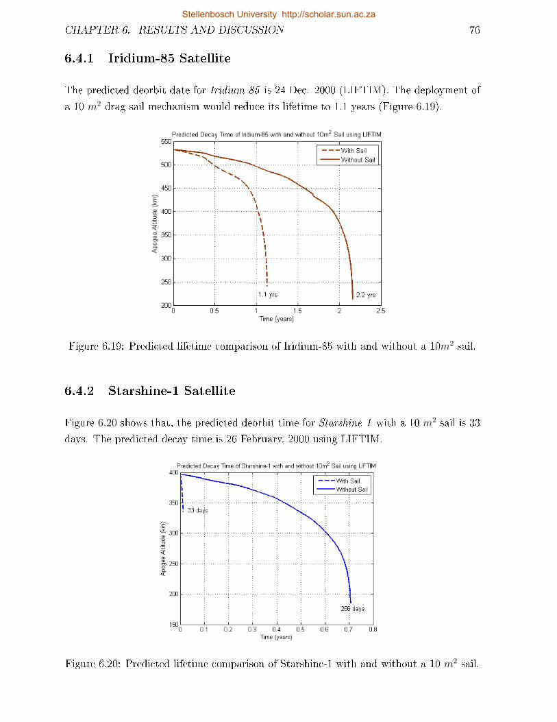
CHAPTER 6. RESULTS AND DISCUSSION 76
6.4.1 Iridium-85 Satellite
The predicted deorbit date for Iridium-85 is 24 Dec. 2000 (LIFTIM). The deployment of
a 10 m2 drag sail mechanism would reduce its lifetime to 1.1 years (Figure 6.19).
Figure 6.19: Predicted lifetime comparison of Iridium-85 with and without a 10m2 sail.
6.4.2 Starshine-1 Satellite
Figure 6.20 shows that, the predicted deorbit time for Starshine-1 with a 10 m2 sail is 33
days. The predicted decay time is 26 February, 2000 using LIFTIM.
Figure 6.20: Predicted lifetime comparison of Starshine-1 with and without a 10 m2 sail.
Stellenbosch University http://scholar.sun.ac.za
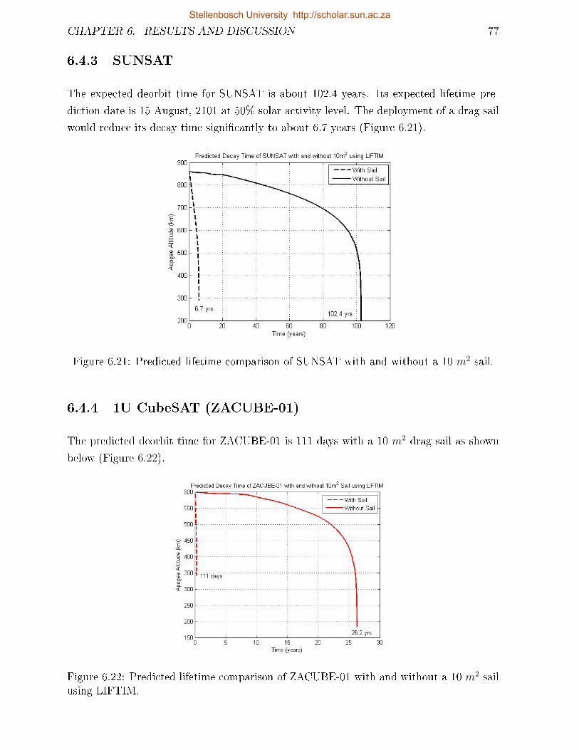
CHAPTER 6. RESULTS AND DISCUSSION 77
6.4.3 SUNSAT
The expected deorbit time for SUNSAT is about 102.4 years. Its expected lifetime pre-
diction date is 15 August, 2101 at 50% solar activity level. The deployment of a drag sail
would reduce its decay time signicantly to about 6.7 years (Figure 6.21).
Figure 6.21: Predicted lifetime comparison of SUNSAT with and without a 10 m2 sail.
6.4.4 1U CubeSAT (ZACUBE-01)
The predicted deorbit time for ZACUBE-01 is 111 days with a 10 m2 drag sail as shown
below (Figure 6.22).
Figure 6.22: Predicted lifetime comparison of ZACUBE-01 with and without a 10 m2 sailusing LIFTIM.
Stellenbosch University http://scholar.sun.ac.za
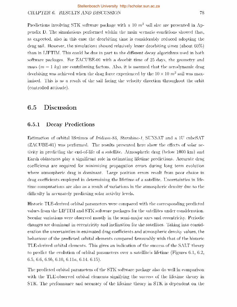
CHAPTER 6. RESULTS AND DISCUSSION 78
Predictions involving STK software package with a 10 m2 sail size are presented in Ap-
pendix D. The simulations performed within the main scenario conditions showed that,
as expected, also in this case the deorbiting time is considerably reduced adopting the
drag sail. However, the simulations showed relatively lesser deorbiting times (about 60%)
than in LIFTIM. This could be due in part to the dierent decay algorithms used in both
software packages. For ZACUBE-01 with a deorbit time of 25 days, the geometry and
mass (m = 1 kg) are contributing factors. Also, it is assumed that the aerodynamic drag
deorbiting was achieved when the drag force experienced by the 10× 10 m2 sail was max-
imised. This is as a result of the sail facing the velocity direction throughout the orbit
(controlled attitude).
6.5 Discussion
6.5.1 Decay Predictions
Estimation of orbital lifetimes of Iridium-85, Starshine-1, SUNSAT and a 1U cubeSAT
(ZACUBE-01) was performed. The results presented here show the eects of solar ac-
tivity in predicting the end-of-life of a satellite. Atmospheric drag (below 1000 km) and
Earth oblateness play a signicant role in estimating lifetime predictions. Accurate drag
coecients are required for minimising propagation errors during long term evolution
where atmospheric drag is dominant. Large position errors result from poor choice in
drag coecients employed in determining the lifetime of a satellite. Uncertainties in life-
time computations are also as a result of variations in the atmospheric density due to the
diculty in accurately predicting solar activity levels.
Historic TLE-derived orbital parameters were compared with the corresponding predicted
values from the LIFTIM and STK software packages for the satellites under consideration.
Secular variations were observed mostly in the semi-major axes and eccentricity. Periodic
changes are dominant in eccentricity and inclination for the satellites. Taking into consid-
eration the uncertainties in estimated drag coecients and atmospheric density values, the
behaviour of the predicted orbital elements compared favourably with that of the historic
TLE-derived orbital elements. This gives an indication of the success of the SALT theory
to predict the evolution of orbital parameters over a satellite's lifetime (Figures 6.1, 6.2,
6.5, 6.6, 6.9b, 6.10, 6.11a, 6.14, 6.15).
The predicted orbital parameters of the STK software package also do well in comparison
with the TLE-observed orbital elements signifying the success of the lifetime theory in
STK. The performance and accuracy of the lifetime theory in STK is dependent on the
Stellenbosch University http://scholar.sun.ac.za
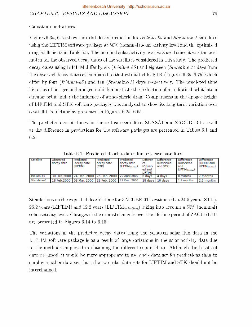
CHAPTER 6. RESULTS AND DISCUSSION 79
Gaussian quadratures.
Figures 6.3a, 6.7a show the orbit decay prediction for Iridium-85 and Starshine-1 satellites
using the LIFTIM software package at 50% (nominal) solar activity level and the optimised
drag coecients in Table 5.5. The nominal solar activity level was used since it was the best
match for the observed decay dates of the satellites considered in this study. The predicted
decay dates using LIFTIM dier by six (Iridium-85 ) and eighteen (Starshine-1 ) days from
the observed decay dates as compared to that estimated by STK (Figures 6.3b, 6.7b) which
dier by four (Iridium-85 ) and ten (Starshine-1 ) days respectively. The predicted time
histories of perigee and apogee radii demonstrate the reduction of an elliptical orbit into a
circular orbit under the inuence of atmospheric drag. Comparisons in the apogee height
of LIFTIM and STK software packages was analysed to show its long-term variation over
a satellite's lifetime as presented in Figures 6.2b, 6.6b.
The predicted deorbit times for the test case satellites, SUNSAT and ZACUBE-01 as well
as the dierence in predictions for the software packages are presented in Tables 6.1 and
6.2.
Table 6.1: Predicted deorbit dates for test case satellites.
Simulations on the expected deorbit time for ZACUBE-01 is estimated at 24.5 years (STK),
26.2 years (LIFTIM) and 12.2 years (LIFTIMSchatten) taking into account a 50% (nominal)
solar activity level. Changes in the orbital elements over the lifetime period of ZACUBE-01
are presented in Figures 6.14 to 6.15.
The variations in the predicted decay dates using the Schatten solar ux data in the
LIFTIM software package is as a result of large variations in the solar activity data due
to the methods employed in obtaining the dierent sets of data. Although, both sets of
data are good, it would be more appropriate to use one's data set for predictions than to
employ another data set thus, the two solar data sets for LIFTIM and STK should not be
interchanged.
Stellenbosch University http://scholar.sun.ac.za
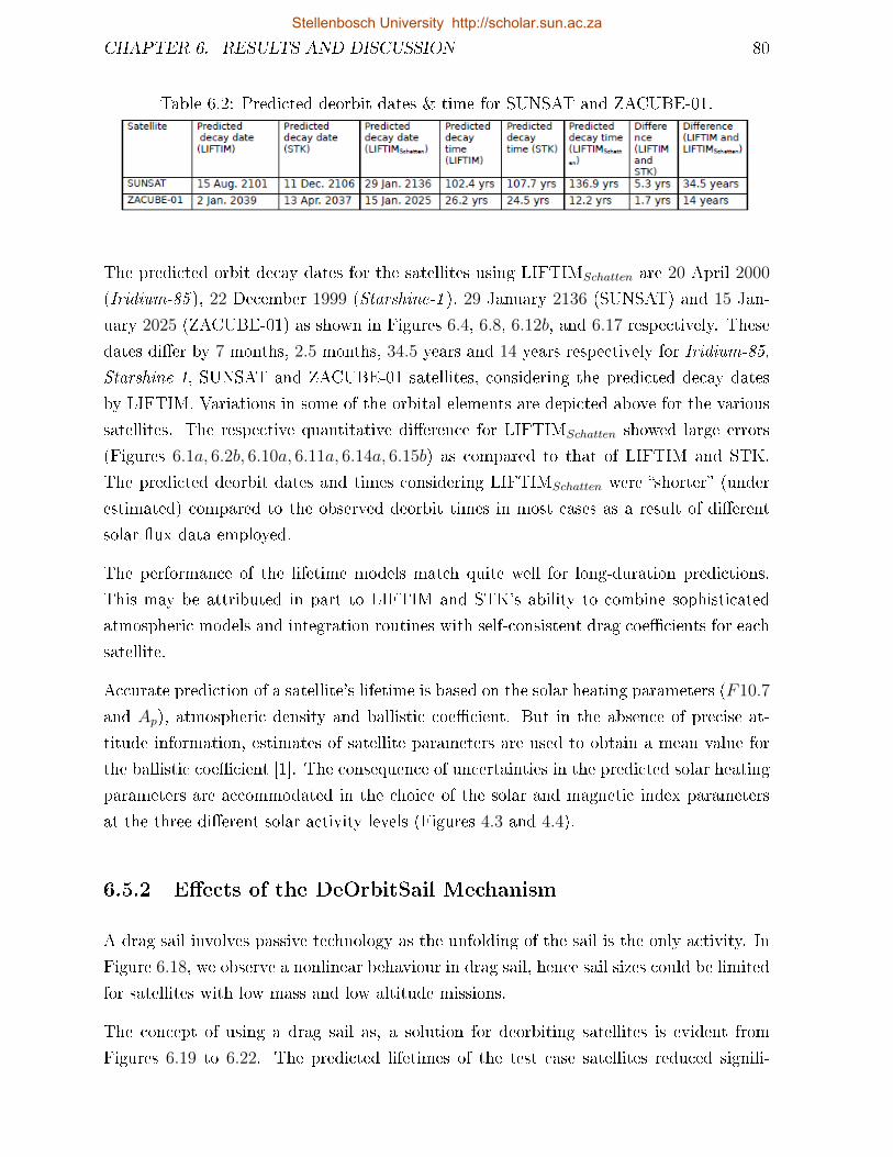
CHAPTER 6. RESULTS AND DISCUSSION 80
Table 6.2: Predicted deorbit dates & time for SUNSAT and ZACUBE-01.
The predicted orbit decay dates for the satellites using LIFTIMSchatten are 20 April 2000
(Iridium-85 ), 22 December 1999 (Starshine-1 ), 29 January 2136 (SUNSAT) and 15 Jan-
uary 2025 (ZACUBE-01) as shown in Figures 6.4, 6.8, 6.12b, and 6.17 respectively. These
dates dier by 7 months, 2.5 months, 34.5 years and 14 years respectively for Iridium-85,
Starshine-1, SUNSAT and ZACUBE-01 satellites, considering the predicted decay dates
by LIFTIM. Variations in some of the orbital elements are depicted above for the various
satellites. The respective quantitative dierence for LIFTIMSchatten showed large errors
(Figures 6.1a, 6.2b, 6.10a, 6.11a, 6.14a, 6.15b) as compared to that of LIFTIM and STK.
The predicted deorbit dates and times considering LIFTIMSchatten were shorter (under
estimated) compared to the observed deorbit times in most cases as a result of dierent
solar ux data employed.
The performance of the lifetime models match quite well for long-duration predictions.
This may be attributed in part to LIFTIM and STK's ability to combine sophisticated
atmospheric models and integration routines with self-consistent drag coecients for each
satellite.
Accurate prediction of a satellite's lifetime is based on the solar heating parameters (F10.7
and Ap), atmospheric density and ballistic coecient. But in the absence of precise at-
titude information, estimates of satellite parameters are used to obtain a mean value for
the ballistic coecient [1]. The consequence of uncertainties in the predicted solar heating
parameters are accommodated in the choice of the solar and magnetic index parameters
at the three dierent solar activity levels (Figures 4.3 and 4.4).
6.5.2 Eects of the DeOrbitSail Mechanism
A drag sail involves passive technology as the unfolding of the sail is the only activity. In
Figure 6.18, we observe a nonlinear behaviour in drag sail, hence sail sizes could be limited
for satellites with low mass and low altitude missions.
The concept of using a drag sail as, a solution for deorbiting satellites is evident from
Figures 6.19 to 6.22. The predicted lifetimes of the test case satellites reduced signi-
Stellenbosch University http://scholar.sun.ac.za
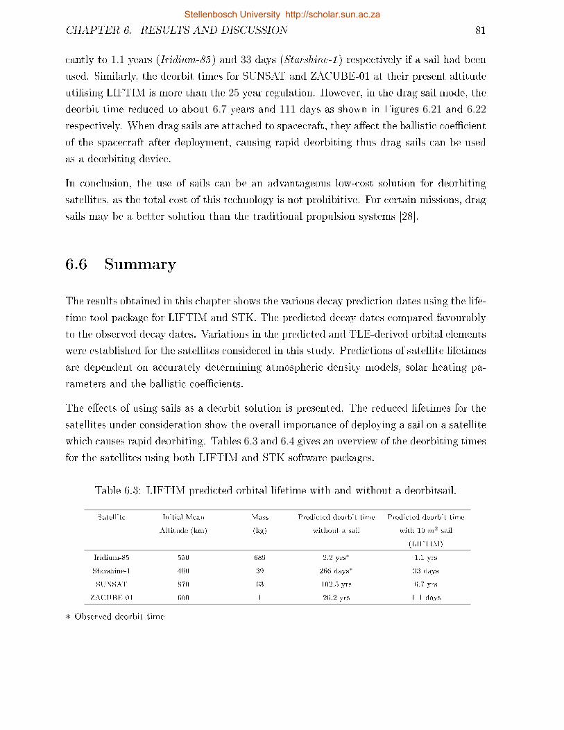
CHAPTER 6. RESULTS AND DISCUSSION 81
cantly to 1.1 years (Iridium-85 ) and 33 days (Starshine-1 ) respectively if a sail had been
used. Similarly, the deorbit times for SUNSAT and ZACUBE-01 at their present altitude
utilising LIFTIM is more than the 25 year regulation. However, in the drag sail mode, the
deorbit time reduced to about 6.7 years and 111 days as shown in Figures 6.21 and 6.22
respectively. When drag sails are attached to spacecraft, they aect the ballistic coecient
of the spacecraft after deployment, causing rapid deorbiting thus drag sails can be used
as a deorbiting device.
In conclusion, the use of sails can be an advantageous low-cost solution for deorbiting
satellites, as the total cost of this technology is not prohibitive. For certain missions, drag
sails may be a better solution than the traditional propulsion systems [28].
6.6 Summary
The results obtained in this chapter shows the various decay prediction dates using the life-
time tool package for LIFTIM and STK. The predicted decay dates compared favourably
to the observed decay dates. Variations in the predicted and TLE-derived orbital elements
were established for the satellites considered in this study. Predictions of satellite lifetimes
are dependent on accurately determining atmospheric density models, solar heating pa-
rameters and the ballistic coecients.
The eects of using sails as a deorbit solution is presented. The reduced lifetimes for the
satellites under consideration show the overall importance of deploying a sail on a satellite
which causes rapid deorbiting. Tables 6.3 and 6.4 gives an overview of the deorbiting times
for the satellites using both LIFTIM and STK software packages.
Table 6.3: LIFTIM predicted orbital lifetime with and without a deorbitsail.
Satellite Initial Mean
Altitude (km)
Mass
(kg)
Predicted deorbit time
without a sail
Predicted deorbit time
with 10 m2 sail
(LIFTIM)
Iridium-85 550 689 2.2 yrs∗ 1.1 yrs
Starshine-1 400 39 266 days∗ 33 days
SUNSAT 870 63 102.5 yrs 6.7 yrs
ZACUBE-01 600 1 26.2 yrs 111 days
∗ Observed deorbit time
Stellenbosch University http://scholar.sun.ac.za
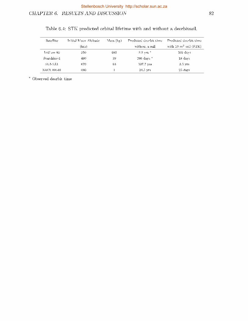
CHAPTER 6. RESULTS AND DISCUSSION 82
Table 6.4: STK predicted orbital lifetime with and without a deorbitsail.
Satellite Initial Mean Altitude
(km)
Mass (kg) Predicted deorbit time
without a sail
Predicted deorbit time
with 10 m2 sail (STK)
Iridium-85 550 689 2.2 yrs ∗ 355 days
Starshine-1 400 39 266 days ∗ 18 days
SUNSAT 870 63 107.7 yrs 3.5 yrs
ZACUBE-01 600 1 24.5 yrs 25 days
∗ Observed deorbit time
Stellenbosch University http://scholar.sun.ac.za
Chapter 7
Conclusion and Future Work
This chapter summarise the content of this study and the overall perspective of this work
is established. The most signicant assumptions and simplications that were made in the
previous chapters are summarised and results evaluated against the initial objectives of this
study. Conclusions are drawn from the results obtained, with further recommendations
based on the results and observations presented.
The objectives as formulated in Chapter one, are repeated here for reference:
1. Investigate the accuracy of predicted orbital element evolution over (test) satellite's
lifetime (re-entry date).
2. Investigate the eects of perturbations on time evolution of satellite orbital elements
and orbital lifetime of SUNSAT.
3. Test the theory and long-term predicted solar and magnetic data sets by implement-
ing relevant algorithms and software packages and comparing the theoretical results
with observed/ historic TLE-derived orbital parameters.
4. Investigate the DeOrbitSail mission to reduce the lifetime of satellites with regards
to deorbiting using aerodynamic drag.
The following sections summarises the results of the study with reference to the above
objectives.
83
Stellenbosch University http://scholar.sun.ac.za
CHAPTER 7. CONCLUSION AND FUTURE WORK 84
7.1 Summary of Study
7.1.1 Lifetime Predictions
Two lifetime prediction models, the Semi-Analytical Liu Theory (SALT) and Satellite
ToolKit (STK) were used in this study. Liu's theory utilised the variational equations of
motion for the orbit mean elements due to the Earth's oblateness and atmospheric drag
only. The satellite toolkit used an n 9-point Gaussian quadrature which integrates the
slowly varying orbital elements over time by integrating over one orbit to determine the
rate-of-change of each variable. A theoretical and numerical foundation of the SALT is
presented in Chapter 4 and provides an ecient simulation tool used in this study.
The rst important aspect in the decay process was established and it was shown that, two
separate parameters (atmospheric drag and earth oblateness) are the main forces which
inuences the decay of near Earth satellites. The perturbing eects on time evolved orbital
elements showed that, atmospheric drag leads to decreasing values of eccentricity (e) and
semi-major axis (a). Apart from the eects on a and e, the perturbation in the trajectory
was also observed in other orbital elements such as the inclination (i) as observed in the
TLE-derived historic orbital elements and predictions using the STK software package.
Variations in apogee (ra) and perigee radius (rp) are bound to aect an orbit substantially.
The apogee and perigee heights are functions of a and e, hence oscillations induced in these
two elements produce a faster decrease in ra than in rp (due to the secular reduction in
eccentricity) associated with a lower ra which will cause a satellite to ultimately enter the
lower atmosphere.
The accuracy of both models was considered next. The software packages were rst
evaluated against the actual orbit decay histories of the test case satellites (Iridium-85
and Starshine-1) prior to applying the solution to SUNSAT's orbit. The comparative
small dierences between the predicted and TLE-observed deorbit dates for the test case
satellites, demonstrated the success of the LIFTIM and STK in predicting satellite lifetime
for these satellites. According to Liu's theory [1], variations in the solar heating parameters
coupled with satellite's ballistic coecient are of greater importance on the prediction
accuracy of a satellite's life span.
A quantitative comparison of the orbital parameters was investigated for the satellites
involved. This showed the error dierence in predictions between the actual TLE decay
histories and the software packages. The relatively small errors gives an indication of the
performance of the software packages. The evolution of the orbital elements other than
the cartesian position of the satellites over their lifetimes was used due to the long orbital
Stellenbosch University http://scholar.sun.ac.za
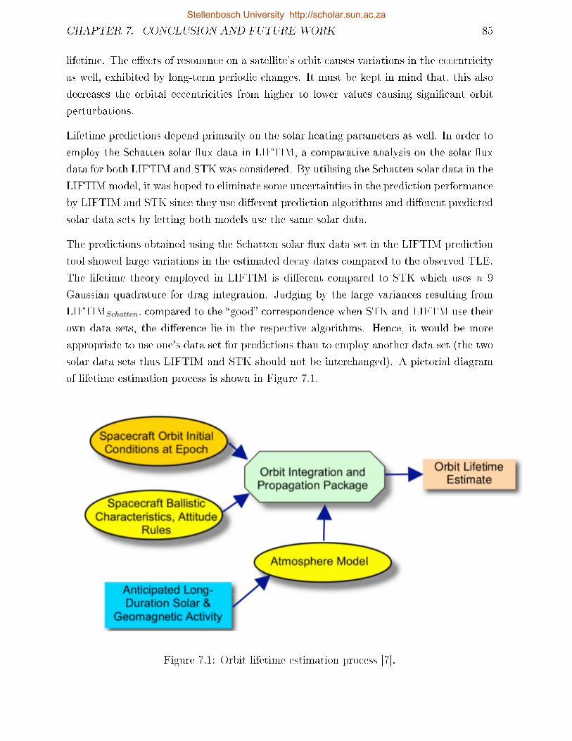
CHAPTER 7. CONCLUSION AND FUTURE WORK 85
lifetime. The eects of resonance on a satellite's orbit causes variations in the eccentricity
as well, exhibited by long-term periodic changes. It must be kept in mind that, this also
decreases the orbital eccentricities from higher to lower values causing signicant orbit
perturbations.
Lifetime predictions depend primarily on the solar heating parameters as well. In order to
employ the Schatten solar ux data in LIFTIM, a comparative analysis on the solar ux
data for both LIFTIM and STK was considered. By utilising the Schatten solar data in the
LIFTIM model, it was hoped to eliminate some uncertainties in the prediction performance
by LIFTIM and STK since they use dierent prediction algorithms and dierent predicted
solar data sets by letting both models use the same solar data.
The predictions obtained using the Schatten solar ux data set in the LIFTIM prediction
tool showed large variations in the estimated decay dates compared to the observed TLE.
The lifetime theory employed in LIFTIM is dierent compared to STK which uses n 9
Gaussian quadrature for drag integration. Judging by the large variances resulting from
LIFTIMSchatten, compared to the good correspondence when STK and LIFTM use their
own data sets, the dierence lie in the respective algorithms. Hence, it would be more
appropriate to use one's data set for predictions than to employ another data set (the two
solar data sets thus LIFTIM and STK should not be interchanged). A pictorial diagram
of lifetime estimation process is shown in Figure 7.1.
Figure 7.1: Orbit lifetime estimation process [7].
Stellenbosch University http://scholar.sun.ac.za
CHAPTER 7. CONCLUSION AND FUTURE WORK 86
Finally, depending on solar activity levels thus 95% (+2sigma) and 50% (nominal), the
estimated lifetime for SUNSAT according to Liu's theory is between 35 and 103 years.
ZACUBE-01 expected lifetime is between 13 and 27 years. STK's estimated lifetime for
SUNSAT is 107.7 years and ZACUBE-01 is 24.5 years.
7.1.2 DeOrbitSail Mechanism
The deorbitsail concept was investigated. The primary aim was to demonstrate the concept
of end-of-life deorbiting using a sail membrane (10 × 10 m2) as a drag sail. We observed
that, in the drag sail mode the satellites have shorter predicted lifetimes than without a
sail. This demonstrated that drag sails could subsequently be used as a deorbiting device
for rapid deorbiting. This technology shows the readiness level of drag sails and hence can
be adapted for use on satellites in the future. The sail deployment can be used as a low
cost solution to reduce the accumulation of space debris in the near future. Appendix E
shows a conguration (stowed and deployed) of a sail membrance.
7.2 Conclusion
In this thesis, the feasibility of predicting satellite lifetimes in LEO by employing two
separate software packages was established. More importantly, investigating the eects
of orbital perturbations on the time evolution of the satellite orbital elements and orbital
lifetime of SUNSAT was ascertained.
The eciency of satellite lifetime predictions depend on the ability to estimate many
variables in combination with sophisticated atmospheric models. These models, though
highly recommended, are still inadequate to account for all the variations of the satellite's
environment that aects the lifetime of satellites especially when using uncertain predicted
values. Studies in atmospheric density modelling, estimation of drag coecient and their
eects on atmospheric drag have produced notable advances in orbital lifetime estimation
models.
LIFTIM and STK prediction tools has been found to be a simplied yet rather accurate
tool in the continuing eort of understanding and estimating a satellite's orbital life. It also
illustrates greater signicance on prediction accuracy taking into account the atmospheric
density model.
The deorbitsail technique allowed for safe deorbiting of spacecraft at the end of their
lifetime. It also addressed the challenge of continual growth of space debris in LEO by
Stellenbosch University http://scholar.sun.ac.za
CHAPTER 7. CONCLUSION AND FUTURE WORK 87
employing sizeable (10 ×10 m2) drag sails to help reduce the accumulation of space junk
in the near future. We also demonstrated that, in a drag sail mode, rapid deorbiting is
enhanced.
7.3 Further Research and Recommendation
The following considerations must be taken into account for improvements in the prediction
process;
The accuracy and execution speed of the numerical integration algorithm of Liu's
model could be compensated by using higher order integrators such as Adams-
Bashforth etc.
The atmospheric density model (Jacchia-70) could also be replaced with a more
sophisticated and accurate model.
A dedicated drag analysis study could be investigated for each satellite based on the
geometry, orbital regime and environmental conditions to be used in the prediction
theory or algorithm.
The need for an improved LIFTIM algorithm.
The performance of Liu's theory should be evaluated for a variety of orbit classes and
satellite lifetimes.
The concept of the deorbitsail mechanism could be further expanded by looking at alter-
natives towards nding a scalable solution for drag sails depending on the size and mass
of the satellite.
Stellenbosch University http://scholar.sun.ac.za

Bibliography
[1] J. J. F. Liu, R. L. Alford, The Orbit Decay and Lifetime (LIFTIM) Prediction Pro-
gram. Northrop Services, Inc., Hunstville, Ala., M-240-21278, May, 1974.
[2] B. Hofmann-Wellenhof, H. Lichtenegger, W. Wasle, GNSS - Global Navigation Satel-
lite Systems, GPS, GLONASS, Galileo and more. 1st ed. New York: Springer-Verlag
Wien, 2008.
[3] V. A. Chobotov, Orbital Mechanics, 3rd ed. AIAA Educational Series, Reston, Vir-
ginia, VA, 2002.
[4] D. A. Vallado, Fundamentals of Astrodynamics and Applications. Space Technology
Series, McGraw-Hill Custom Publishing, New York, 1997.
[5] J. J. Sellers, W. J. Larson, R. B. Gien, W. J. Astore, Understanding Space: An
Introduction to Astronautics. Revised 2nd ed. Space Technology Series, McGraw-Hill
Custom Publishing, New York, NY, 2004.
[6] R. Bate, D. D. Mueller, J. E. White, Fundamentals of Astrodynamics. 1st ed, Dover
Publications, Inc, New York, NY, 1971.
[7] Space Systems, Determining orbit lifetime, ISO copyright oce, CH-1211, ISO/TC
20/SC 14 27852, Geneva20, 2007.
[8] [Online]. Available: http//sail.msfc.nasa.gov/nse/solar.html. [accessed 3 March,
2012].
[9] R. Sandau, K. Brieβ., Reasons for satellite mission miniaturisation and its conse-
quences. Acta Astronautica, Elsevier, Vol 43, Issues 11 -12, 1998, pp. 583 - 596,
http://dx.doi.org/10.1016/S0094-5765(99)00007-7.
[10] T. S. Kelso, NORAD Two-Line Element Sets, Current Data. [Online]. Available:
http://celestrak.com/NORAD/elements/. [accessed 20 August, 2011].
88
Stellenbosch University http://scholar.sun.ac.za
BIBLIOGRAPHY 89
[11] [Online]. Available: https://www.space-track.org/perl/home.pl. [accessed 3 April,
2012].
[12] B. D. L. Opperman, Precision Propagation and Orbit Decay Prediction of Low Earth
Orbit Satellites. M.Sc. Thesis. University of Stellenbosch, Stellenbosch, South Africa,
2003.
[13] F. R. Hoots, R. L. Roehrich, T. S. Kelso, Models for Propagation of NORAD Ele-
ment Sets. Spacetrack report no.3. Defense Documentation Center Cameron Station,
Alexandria, VA 22314. 1988.
[14] H. Klinkrad, Space Debris - Models and Risk Analysis. Springer, Verlag, Berlin, Hei-
delberg, New York. 2006.
[15] J. C. Liou, N. Johnson, N. Hill, Controlling the Growth of Future LEO Debris Pop-
ulation with Active Debris Removal. Acta Astronautica, Vol. 66 No. 5-6, 2010, pp.
648-653, doi:10.1016/j.actaastro.2009.08.05. [accessed 15 February, 2012]
[16] NASA HANDBOOK, Handbook for Limiting Orbital Debris: Measurement System
Identication metric. [Online]. Available: http://www.hq.nasa.gov/oce/codeq/ doc-
tree/NHBK871914.pdf. [accessed 6 November, 2011]
[17] Anon., Inter-Agency Space Debris Coordination Committee, Space Debris Mitigation
Guidelines. Issue 1, Rev.1, 2002a.
[18] NASA Safety Standard: Guidelines and Assessment Procedures for Limiting Orbital
Debris. NSS 1740.14. August, 1995.
[19] J-C. Liou, N. L. Johnson, Risks in Space from Orbiting Debris. Science, Vol. 311, pp.
342 - 341, 20th January, 2006.
[20] Anon., Monthly Number of Cataloged Objects in Earth Orbit by Object Type. Chart,
The Orbital Debris Quartely News, NASA JSC , p.10, January 2011. [Online].
Available: http://www.orbitaldebris.jsc.nasa.gov/newsletter/pfds/ODQNv15i1.pdf.
[12 April, 2012]
[21] H. Klinkrad, P. Beltrami, S. Hauptmann, C. Martin, H. Sdunnus, H. Stokes, R.
Walker, J. Wilkinson, ESA Space Debris Mitigation Handbook. Advances in Space,
Vol. 34, Issue 5, pp 1251- 1259, 2004. http//dx.doi.org/10.1016/j.asr.2003.01.018.
[22] NASA Orbital Debris Program Oce, Orbital Debris Mitigation. [Online]. Avail-
able. http://www.orbitaldebris.jsc.nasa.gov/mitigate/mitigation.html. [accessed 10
September, 2011]
Stellenbosch University http://scholar.sun.ac.za
BIBLIOGRAPHY 90
[23] U. S. Government Orbital Debris Mitigation Standard Practices. [Online]. Avail-
able. http://orbitaldebris.jsc.nasa.gov/library/USG_OD_Standard_Practices.pdf. [
15 January, 2012]
[24] Federal Communications Commission, In the Matter of Mitigation of Orbital Debris.
FCC 04-130, Washington, DC, pp. 2, June 2004.
[25] C. R. McInnes, Solar Sailing: Orbital Mechanics and Mission Applications. Advance
in Space Research, Vol. 31, No. 8, pp. 1971 - 1980, 2003.
[26] C. R. McInnes, Solar Sailing: Technology, Dynamics and Mission Applications,
Springer-Verlag Series in Space Science and Technology, Springer-Verlag, Praxis,1999.
[27] B. Wie, Solar Sail Attitude Control and Dynamics, Parts 1 and 2. Journal of Guid-
ance, Control and Dynamics, Vol. 27, No.4, pp. 526- 544, July-August, 2004.
[28] V. Lappas, N. Adeli, L. Visagie, J. Fernandez, T. Theodorou, W. Steyn, M. Perren,
CubeSail: A low cost CubeSat based solar sail demonstration mission. Advances in
Space Research, 48 , pp. 1890 - 1901. 2011. http://doi:10.1016/j.asr.2011.05.033.
[29] J. Amos, Mini-camera pictures Japan's Ikaros solar sail. [Online]. Available.
http://www.bbc.co.uk/news/10328584. [12 April, 2012]
[30] J. R. Wertz, D. F. Everett, J. J. Puschell, Space Mission Engineering: The New
SMAD, Space Technology Library, Microcosm Press, Hawthorne, CA, 2011.
[31] K. Alfriend, S. R. Vadali, P. Gurl, J. How, L. Breger, Spacecraft Formation Fly-
ing: Dynamics, Control, and Navigation. 1st ed, Elsevier Astrodynamics Series,
Butterworth-Heinemann Publication, 2010.
[32] F. R. Hoots, R. L. Roehrich, T. S. Kelso, Models for Propagation of NORAD Ele-
ment Sets. Spacetrack report no. 3. Defense Documentation Center Cameron Station
Alexandria VA 22314. 1988.
[33] D. G. King-Hele, Satellite Orbits in an Atmosphere, Theory and Applications. Blackie
and Sons Ltd, pp 10 - 11, 1987.
[34] P. R. Escobal, Methods of Orbit Determination, 2nd ed, Krieger Publishing Company,
Malabar, Florida, 1985.
[35] [Online].Available:www.fas.org/spp/guide/china/earth/fy-1.htm. [accessed 18 May,
2012].
Stellenbosch University http://scholar.sun.ac.za
BIBLIOGRAPHY 91
[36] O. Montenbruck, E. Gill, Satellite Orbits: Models, Methods, Applications. 1st ed,
Springer, 2000.
[37] K. E. Tsiolkovsky, Extension of Man into Outer Space, 1921 [also, Tsiolkovsky, K. E.,
Symposium Jet Propulsion, No. 2, United Scientic and Technical Presses, 1936].
[38] K. Tsander, From a Scientic Heritage, NASA Technical Translation TTF-541, 1967
[quoting a 1924 report by the author].
[39] [Online]. Available: www.nasa.gov/mission_pages/smallsats/11-148.html. [accessed
20 October, 2011].
[40] J. J. F. Liu, A Second-order Theory of an Articial Satellite under the Inuence of
the Oblateness of the Earth. AIAA 12th Aerospace Sciences meeting, AIAA paper,
pp. 74 - 166, January, 30 - February 1st, 1974.
[41] J. J. F. Liu, R. L Alford, An Introduction to Gauss-Legendre Quadrature, Northrop
Services, Inc., Huntsville Ala., M-240-1288, October, 1973.
[42] FP7 DeOrbitSail Kicko Meeting, University of Surrey, Guildford, Surrey, United
Kingdom, June 3, 2011.
[43] NASA Orbital Debris Program Oce, Orbital Debris Remediation. [Online]. Avail-
able.http:// www.orbitaldebris.jsc.nasa.gov/Remediation/remediation.html.[15 May,
2012].
[44] Analytical Graphics, Inc. [Online]. Available: http://www.agi.com/products/stk/Defa
ult.aspc. [accessed 20 October, 2012].
[45] Analytical Graphics, Inc. [Online]. Available: ftp://ftp.agi.com/pub/DynamicEarthDa
ta/. [accessed 20 October, 2012].
[46] Analytical Graphics, Inc. [Online]. Available: http://www.agi.com/resources/help/on
line/stk/source/stk/importles-15.htm. [accessed 20 October, 2012].
[47] Analytical Graphics, Inc. [Online]. Available: http://www.agi.com/resources/help/on
line/stk/source/stk/tools-11.htm. [accessed 20 October, 2012].
[48] [Online]. Available: www.swpc.noaa.gov/ftpmenu/indices/old_indices.html. [5 Octo-
ber, 2012].
[49] K. O. Niehuss, H. C. Euler, W. W. Vaughan, Statistical Technique for Intermedi-
ate and Long-Range Estimation of 13-Month Smoothed Solar Flux and Geomagnetic
Index. NASA Technical Memorandum 4759, Marshall Space Flight Center. MSFC,
Alabama 35912. September, 1996.
Stellenbosch University http://scholar.sun.ac.za
BIBLIOGRAPHY 92
[50] [Online]. Available: www.cput.ac.za/les/images_folder/news/news/newsletters/mojo
/Moja %20Newsletter%20October%202011.pdf. [20 October, 2012].
[51] J. J. F. Liu, R. L. Alford, Semi-analytic Theory for a Close-Earth Articial Satellite.
Journal of Guidance and Control, Vol 3, No. 6, pp. 304-311, July-Aug, 1980.
[52] J. J. F. Liu, Satellite Motion About an Oblate Earth. AIAA Journal, Vol. 12, pp.
1511-1516, Nov. 1974.
[53] Y. Kozai, The Motion of a Close Earth Satellite. Astronomical Journal, Vol. 64, pp.
367, Oct. 1959.
[54] D. Brouwer, Solution of the Problem of Articial Satellite Theory Without Drag.
Astronomical Journal, Vol 64, pp. 378-397, Nov. 1959.
[55] H. D. Curtis., Orbital Mechanics for Engineering Students. 2nd ed, Elsevier Aerospace
Engineering Series, Butterworth-Heinemann, Burlington, MA 01803, USA, 2010.
[56] [Online]. Available: www.positim.com/navsys_overview.html. [ 10 November, 2012].
[57] C. C. Chao, R. A. Gick., Long-term evolution of navigation satellite orbits:
GPS/GLONASS/GALILEO. Advances in Space Research, Vol. 34, 1221-1226, 2004.
Stellenbosch University http://scholar.sun.ac.za
Appendix A
Derivation of Equations of Motion
This chapter contains the mathematical derivations of the two-body problem and constants
of motion, as described in chapter 3.
A.1 Two-Body Problem
The two-body motion is derived according to the assumptions stated in section 3.2.1.
Consider a system of two bodies of masses, M and m, as illustrated in Figure 3.3. Their
position vectors with respect to an inertial frame are RM and Rm.
The general two-body problems results if R 6= 0 [3]. Then for mass, M ,
MRM =GMmR
R3(A.1)
and for mass, m,
mRm = −GMmR
R3(A.2)
Subtracting equations. (A.2) from (A.1) yields
R = −G(M +m)
R3R (A.3)
In a restricted two-body problem the principal mass M is assumed xed in inertial space
and m << M , so that m does not aect the motion of M [3]. Dene the gravitational
93
Stellenbosch University http://scholar.sun.ac.za
APPENDIX A. DERIVATION OF EQUATIONS OF MOTION 94
parameter µ with G(M +m) ∼= GM = µ. Therefore, from equation (A.3), therefore [3]
R +GMR
R3= 0 (A.4)
R +µ
R3R = 0 (A.5)
where µ ≡ GM , thus the gravitational parameter.
A.2 Specic Mechanical Energy is a Constant
The two-body equation of motion is given by equation (3.2) as
R +µ
R3R = 0
take the dot product of both sides with R [5],
R •(R +
µ
R3R)
= R • 0
or
R • R +µ
R3R • R = 0 • R = 0
note: R = V and R = V so
V • V +µ
R3R • R = 0 (A.6)
in general, for any two vectors a and b,
a • b = ab cos θ
where θ is the angle between the two vectors.
Assume a is parallel to itself and the angle between them is 0 and cos θ = 1, then
a • a = a2 (A.7)
Take the derivative of both sides of equation (A.7), thus
d
dt(a • a) =
d
dt(a2)
Stellenbosch University http://scholar.sun.ac.za
APPENDIX A. DERIVATION OF EQUATIONS OF MOTION 95
and applying the chain rule of calculus, the derivative becomes
a • a = aa (A.8)
Rewriting equation (A.8) as
VV +µ
R3RR = 0
or
VV +µ
R2R = 0 (A.9)
Take the derivative of equation A.9, we recognise that,
d
dt
(V2
2
)= VV
d
dt
(−µ
R
)=
µ
R2R
hence,d
dt
(V 2
2− µ
R
)= 0 (A.10)
The term in parenthesis is the specic mechanical energy, ε
ε =V 2
2− µ
R(A.11)
ifd
dt(ε) = 0, the ε = constant since we get a constant of integration after integrating the
the dierential equation [5].
A.3 Specic Angular Momentum is a Constant
Take the cross product of the two-body equation of motion with the position vector, R
[5]:
R×(R +
µ
R3R)
= R× 0
R× R +µ
R3(R×R) = 0
The cross product of parallel vectors is zero, hence second term goes to zero and we have
R× R = 0 (A.12)
Stellenbosch University http://scholar.sun.ac.za
APPENDIX A. DERIVATION OF EQUATIONS OF MOTION 96
Now realise thatd
dt(R× R) = (R× R) + (R× R)
where R× R = 0 , hence we have [5]
d
dt(R× R) = R× R
substituting this quantity into equation (A.12), we obtain
d
dt(R× R) = 0
but R = V, therefored
dt(R× V) = 0 (A.13)
recall from equation (3.7), the specic angular momentum is
h = R× V
thus,d
dt(h) = 0 (A.14)
integrating both sides of this equation, we have [5]
h = constant
Stellenbosch University http://scholar.sun.ac.za
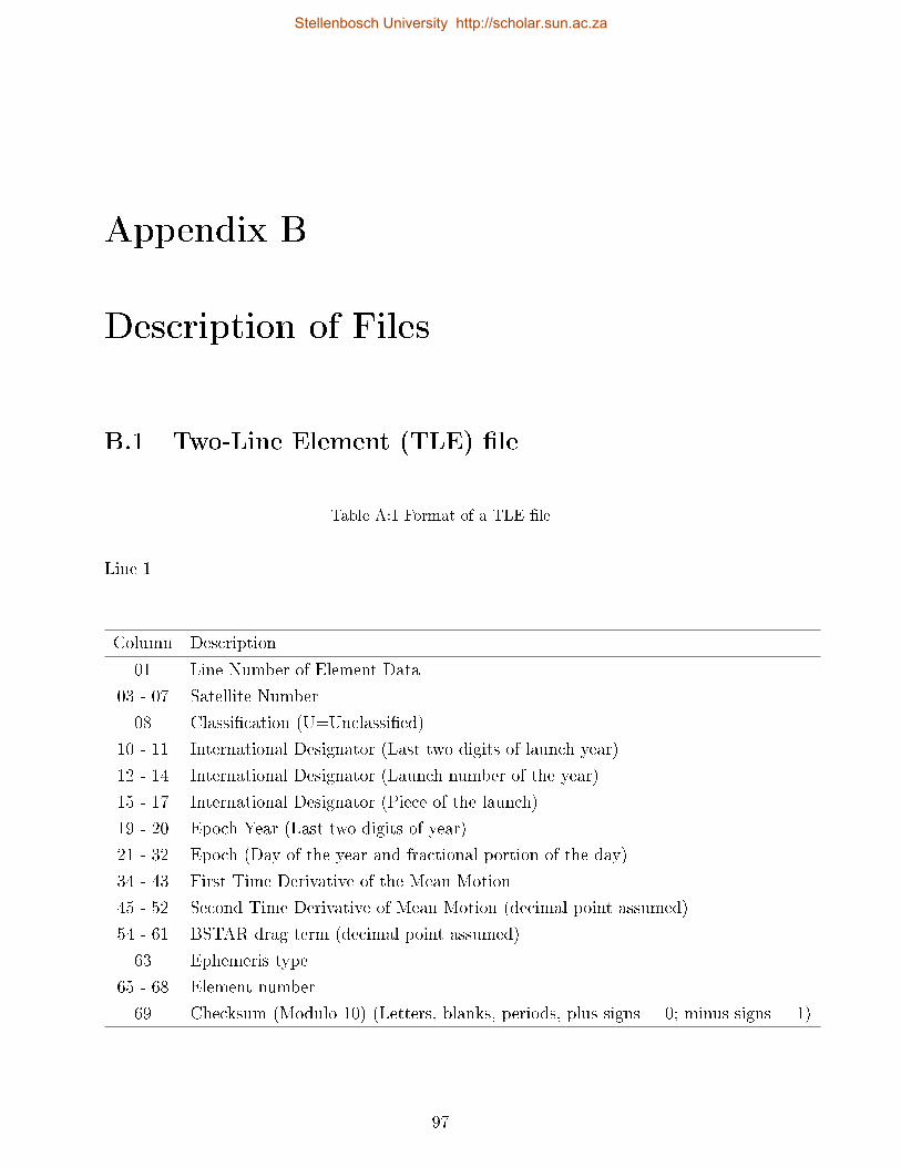
Appendix B
Description of Files
B.1 Two-Line Element (TLE) le
Table A:1 Format of a TLE le
Line 1
Column Description
01 Line Number of Element Data
03 - 07 Satellite Number
08 Classication (U=Unclassied)
10 - 11 International Designator (Last two digits of launch year)
12 - 14 International Designator (Launch number of the year)
15 - 17 International Designator (Piece of the launch)
19 - 20 Epoch Year (Last two digits of year)
21 - 32 Epoch (Day of the year and fractional portion of the day)
34 - 43 First Time Derivative of the Mean Motion
45 - 52 Second Time Derivative of Mean Motion (decimal point assumed)
54 - 61 BSTAR drag term (decimal point assumed)
63 Ephemeris type
65 - 68 Element number
69 Checksum (Modulo 10) (Letters, blanks, periods, plus signs = 0; minus signs = 1)
97
Stellenbosch University http://scholar.sun.ac.za
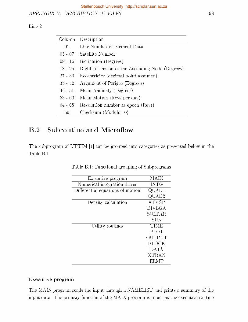
APPENDIX B. DESCRIPTION OF FILES 98
Line 2
Column Description
01 Line Number of Element Data
03 - 07 Satellite Number
09 - 16 Inclination (Degrees)
18 - 25 Right Ascension of the Ascending Node (Degrees)
27 - 33 Eccentricity (decimal point assumed)
35 - 42 Argument of Perigee (Degrees)
44 - 51 Mean Anomaly (Degrees)
53 - 63 Mean Motion (Revs per day)
64 - 68 Revolution number at epoch (Revs)
69 Checksum (Modulo 10)
B.2 Subroutine and Microow
The subprogram of LIFTIM [1] can be grouped into categories as presented below in the
Table B.1
Table B.1: Functional grouping of Subprograms
Executive program MAINNumerical integration driver INTG
Dierential equations of motion QUAD1QUAD2
Density calculation ATMSPBIVLGASOLPARSUN
Utility routines TIMEPLOT
OUTPUTBLOCKDATAXTRANELMT
Executive program
The MAIN program reads the input through a NAMELIST and prints a summary of the
input data. The primary function of the MAIN program is to act as the executive routine
Stellenbosch University http://scholar.sun.ac.za
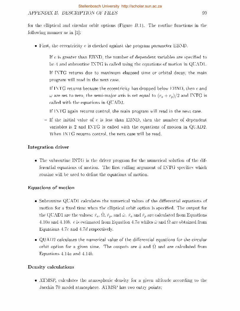
APPENDIX B. DESCRIPTION OF FILES 99
for the elliptical and circular orbit options (Figure B.1). The routine functions in the
following manner as in [1]:
First, the eccentricity e is checked against the program parameter EBND.
If e is greater than EBND, the number of dependent variables are specied to
be 4 and subroutine INTG is called using the equations of motion in QUAD1.
If INTG returns due to maximum elaspsed time or orbital decay, the main
program will read in the next case.
If INTG returns because the eccentricity has dropped below EBND, then e and
ω are set to zero, the semi-major axis is set equal to (ra + rp)/2 and INTG is
called with the equations in QUAD2.
If INTG again returns control, the main program will read in the next case.
If the initial value of e is less than EBND, then the number of dependent
variables is 2 and INTG is called with the equations of motion in QUAD2.
When INTG returns control, the next case will be read.
Integration driver
The subroutine INTG is the driver program for the numerical solution of the dif-
ferential equations of motion. The rst calling argument of INTG species which
routine will be used to dene the equations of motion.
Equations of motion
Subroutine QUAD1 calculates the numerical values of the dierential equations of
motion for a xed time when the elliptical orbit option is specied. The output for
the QUAD1 are the values: ra, Ω, rp, and ω. ra and rp are calculated from Equations
4.10a and 4.10b. e is estimated from Equation 4.7a whiles ω and Ω are obtained from
Equations 4.7c and 4.7d respectively.
QUAD2 calculates the numerical value of the dierential equations for the circular
orbit option for a given time. The outputs are a and Ω and are calculated from
Equations 4.14a and 4.14b.
Density calculations
ATMSP, calculates the atmospheric density for a given altitude according to the
Jacchia 70 model atmosphere. ATMSP has two entry points;
Stellenbosch University http://scholar.sun.ac.za
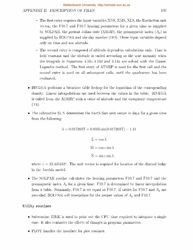
APPENDIX B. DESCRIPTION OF FILES 100
The rst entry requires the input variables XNS, XMS, XLS, the Earth-Sun unit
vector, the F10.7 and F10.7 heating parameters for a given time as supplied
by SOLPAR, the present Julian date (XMJD), the geomagnetic index (Ap) as
supplied by SOLPAR and the day number (DD). These input variables depend
only on time and not altitude.
The second entry is composed of altitude dependent calculations only. Time is
held constant and the altitude is varied according to the true anomaly when
the integrals in Equations 4.10c, 4.10d and 4.14a are solved with the Gauss-
Legendre method. The rst entry of ATMSP is used for the rst call and the
second entry is used on all subsequent calls, until the quadrature has been
evaluated.
BIVLGA performs a bivariate table lookup for the logarithm of the corresponding
density. Linear interpolations are used between the values in the table. BIVLGA
is called from the ATMSP with a value of altitude and the exospheric temperature
(T4).
The subroutine SUN determines the Earth-Sun unit vector in days for a given time
from the following:
λ = 0.017203T + 0.0335 sin(0.017203T)− 1.41
L = cosλ
M = cos ε sinλ
N = sin ε sinλ
where ε = 23.445433o. The unit vector is required for location of the diurnal bulge
in the Jacchia model.
The SOLPAR routine calculates the heating parameters F10.7 and F10.7 and the
geomagnetic index Ap for a given time. F10.7 is determined by linear interpolation
from a table. Nominally, F10.7 is set equal to F10.7. If tables for F10.7 and Ap are
provided, SOLPAR will interpolate for the proper values of Ap and F10.7.
Utility routines
Subroutine TIME is used to print out the CPU time required to integrate a single
case. It also evaluates the eects of changes in program parameters.
PLOT handles the interface for plot routines.
Stellenbosch University http://scholar.sun.ac.za
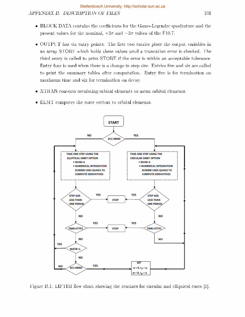
APPENDIX B. DESCRIPTION OF FILES 101
BLOCK DATA contains the coecients for the Gauss-Legendre quadrature and the
present values for the nominal, +2σ and −2σ values of the F10.7.
OUTPUT has six entry points. The rst two entries place the output variables in
an array STORE which holds these values until a truncation error is checked. The
third entry is called to print STORE if the error is within an acceptable tolerance.
Entry four is used when there is a change in step size. Entries ve and six are called
to print the summary tables after computation. Entry ve is for termination on
maximum time and six for termination on decay.
XTRAN converts osculating orbital elements to mean orbital elements.
ELMT computes the state vectors to orbital elements.
Figure B.1: LIFTIM ow chart showing the routines for circular and elliptical cases [1].
Stellenbosch University http://scholar.sun.ac.za
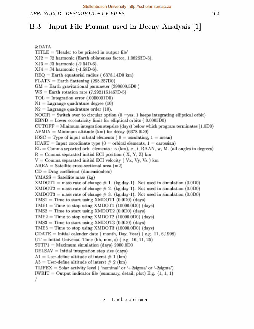
APPENDIX B. DESCRIPTION OF FILES 102
B.3 Input File Format used in Decay Analysis [1]
D = Double precision
Stellenbosch University http://scholar.sun.ac.za
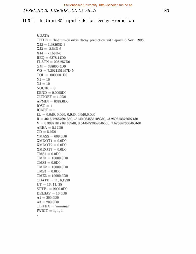
APPENDIX B. DESCRIPTION OF FILES 103
B.3.1 Iridium-85 Input File for Decay Prediction
Stellenbosch University http://scholar.sun.ac.za
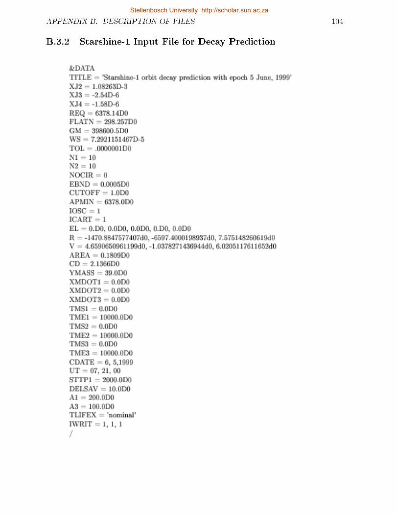
APPENDIX B. DESCRIPTION OF FILES 104
B.3.2 Starshine-1 Input File for Decay Prediction
Stellenbosch University http://scholar.sun.ac.za
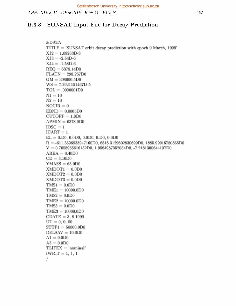
APPENDIX B. DESCRIPTION OF FILES 105
B.3.3 SUNSAT Input File for Decay Prediction
Stellenbosch University http://scholar.sun.ac.za
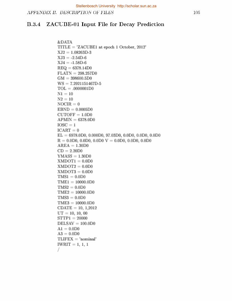
APPENDIX B. DESCRIPTION OF FILES 106
B.3.4 ZACUBE-01 Input File for Decay Prediction
Stellenbosch University http://scholar.sun.ac.za
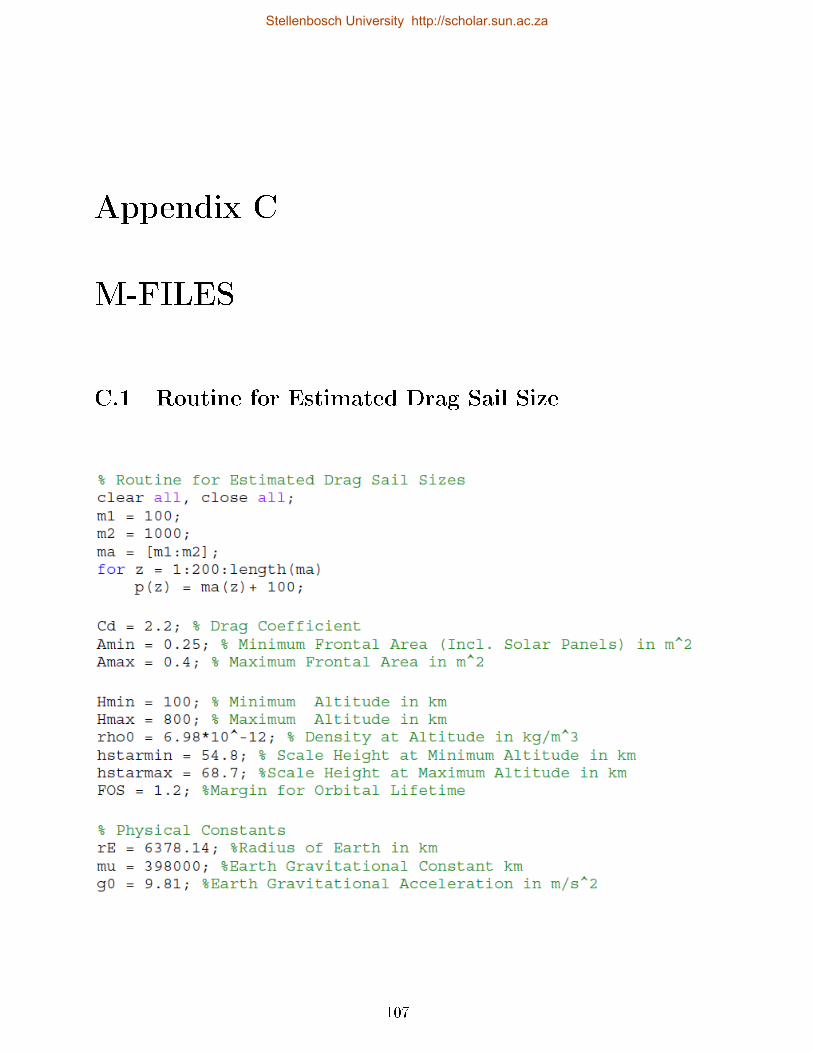
Appendix C
M-FILES
C.1 Routine for Estimated Drag Sail Size
107
Stellenbosch University http://scholar.sun.ac.za
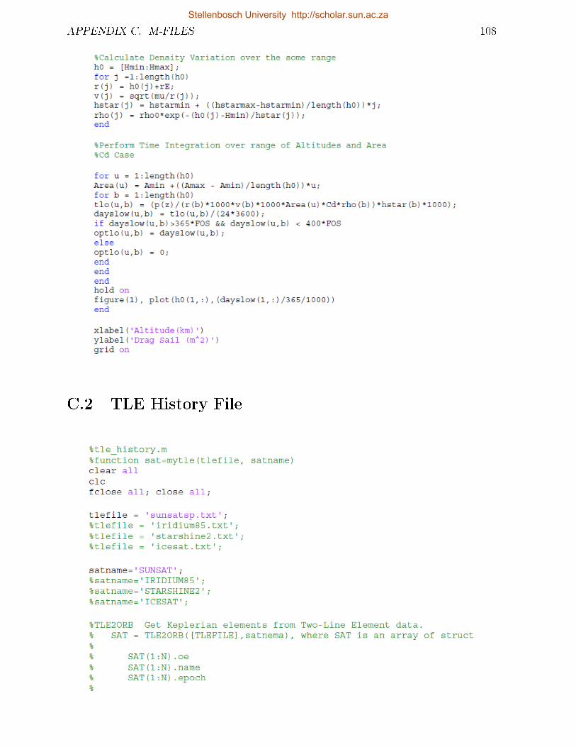
APPENDIX C. M-FILES 108
C.2 TLE History File
Stellenbosch University http://scholar.sun.ac.za
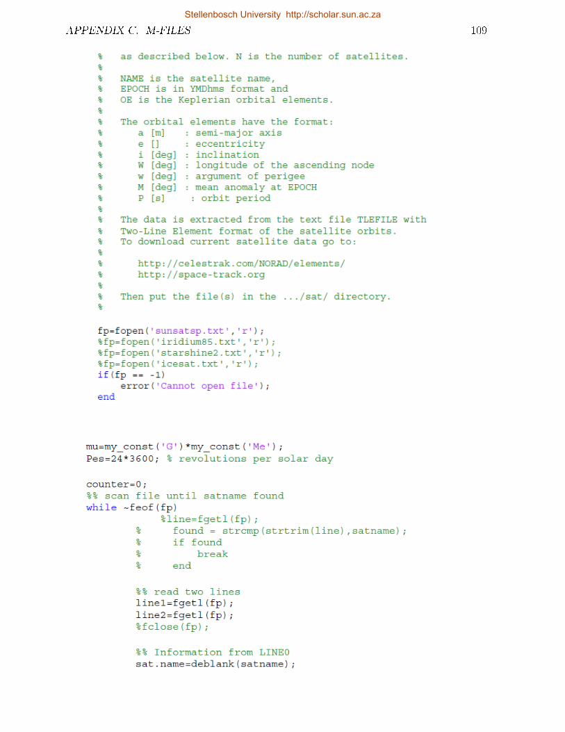
APPENDIX C. M-FILES 109
Stellenbosch University http://scholar.sun.ac.za
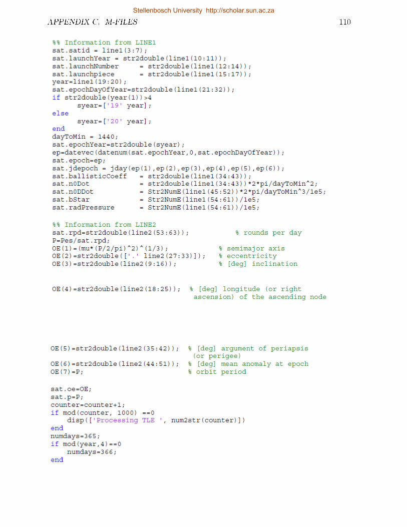
APPENDIX C. M-FILES 110
Stellenbosch University http://scholar.sun.ac.za
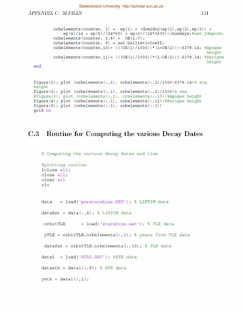
APPENDIX C. M-FILES 111
C.3 Routine for Computing the various Decay Dates
Stellenbosch University http://scholar.sun.ac.za
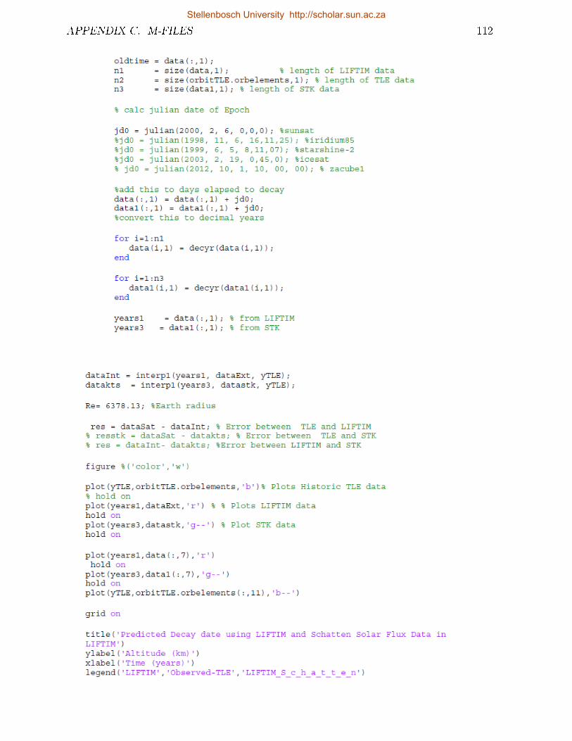
APPENDIX C. M-FILES 112
Stellenbosch University http://scholar.sun.ac.za
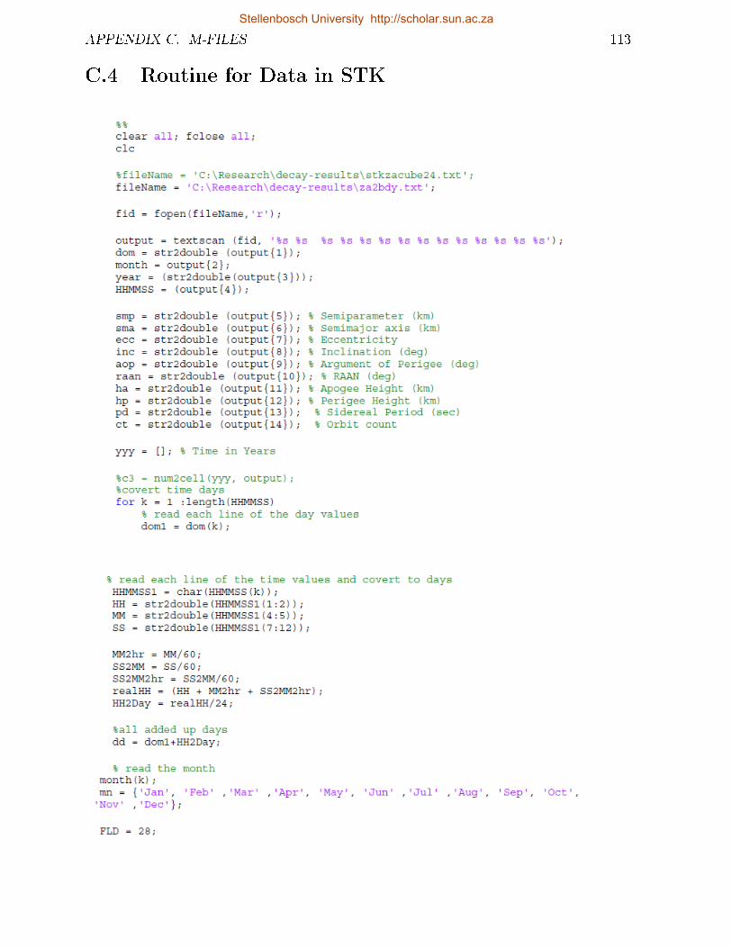
APPENDIX C. M-FILES 113
C.4 Routine for Data in STK
Stellenbosch University http://scholar.sun.ac.za
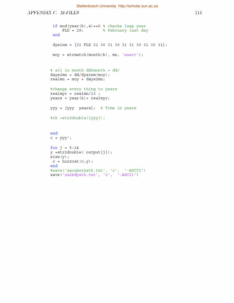
APPENDIX C. M-FILES 114
Stellenbosch University http://scholar.sun.ac.za
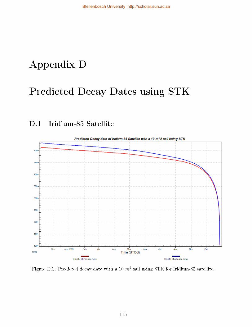
Appendix D
Predicted Decay Dates using STK
D.1 Iridium-85 Satellite
Figure D.1: Predicted decay date with a 10 m2 sail using STK for Iridium-85 satellite.
115
Stellenbosch University http://scholar.sun.ac.za
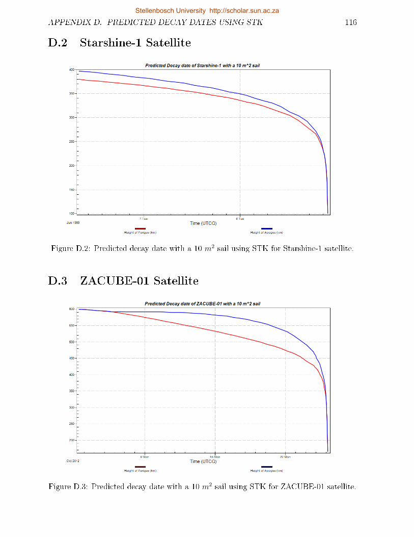
APPENDIX D. PREDICTED DECAY DATES USING STK 116
D.2 Starshine-1 Satellite
Figure D.2: Predicted decay date with a 10 m2 sail using STK for Starshine-1 satellite.
D.3 ZACUBE-01 Satellite
Figure D.3: Predicted decay date with a 10 m2 sail using STK for ZACUBE-01 satellite.
Stellenbosch University http://scholar.sun.ac.za
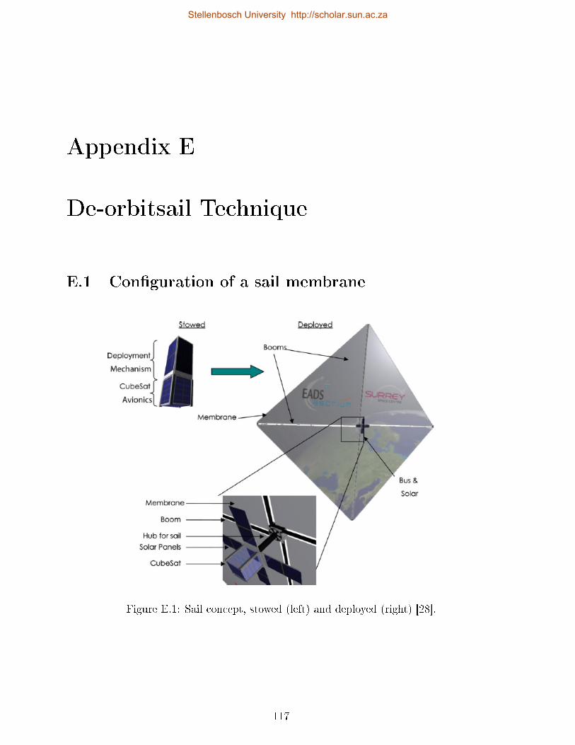
Appendix E
De-orbitsail Technique
E.1 Conguration of a sail membrane
Figure E.1: Sail concept, stowed (left) and deployed (right) [28].
117
Stellenbosch University http://scholar.sun.ac.za
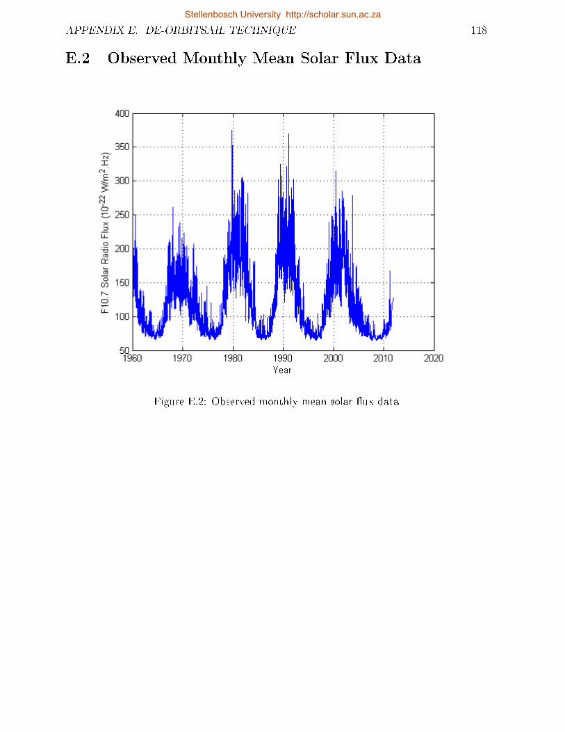
APPENDIX E. DE-ORBITSAIL TECHNIQUE 118
E.2 Observed Monthly Mean Solar Flux Data
Figure E.2: Observed monthly mean solar ux data
Stellenbosch University http://scholar.sun.ac.za


