Partial Differential Lectures Dr. Hussain Ali Mohamad

Third Class

Chapter 1: Introduction

1.1 Notation and Definitions,

1.2 Initial and Boundary Conditions,

1.3 Classification of Second Order Equations,

1.4 Some Known Equations,

1.5 Superposition Principle,

Chapter 2: Method of Characteristics

First Order Equations,

2.1 Linear Equations with Constant Coefficients,

2.2 Linear Equations with Variable Coefficients,

2.3 First Order Quasi-linear Equations,

2.4 First Order Nonlinear Equations,

2.5 Geometrical Considerations,

2.6 Some Theorem on Characteristics,

Second Order Equations,

2.7 Linear and Quasi-linear Equations,

Chapter 3: Linear Equations with Constant Coefficients

3.1 Inverse Operators,

3.2 Homogeneous Equations,

3.3 Nonhomogeneous Equations,

Chapter 4: Orthogonal Expansions,

4.1 Orthogonality,

4.2 Orthogonal Polynomials,

4.3 Series of Orthogonal Functions,

1.1 Notation and Definitions

Definitions about order, linearity, homogeneity, and solutions for partial

differential equations resemble those in the case of ordinary differential equations

and are as follows: The order of a partial differential equation is the same

as the order of the highest derivative appearing in the equation. The partial derivatives

are sometimes denoted by , or and respectively. The most

general first order partial differential equation with two independent variables and is

written in the form

( ) ( )

The most general second order partial differential equation is of the form

( ) ( ) 2

A partial differential equation is said to be linear if the unknown function

u and all its partial derivatives appear in an algebraically linear form, i.e., of

the first degree. For example, the equation

( )

where the coefficients , and and the function are

functions of x and y, is a second order linear partial differential equation in the unknown

( ). An operator is a linear differential operator iff

( ) , where and are scalars, and and are any functions

with continuous partial derivatives of appropriate order .

A partial differential equation is said to be homogeneous, whereas , where

L is any differential operator and 5 7^ 0 is a given function of the independent variables, is

said to be nonhomogeneous. For example

( ) (

)

is a nonhomogeneous first order linear equation, whereas

* )

is homogeneous. Thus, a linear homogeneous equation is such that whenever

u is a solution of the equation, then cu is also a solution where c is a constant .

A function is said to be a solution of a partial differential equation if and its

partial derivatives, when substituted for u and its partial derivatives occurring in the partial

differential equation, reduce it to an identity in the independent variables. The general

solution of a partial differential equation is a linear combination of all solutions of the

equation with as many arbitrary functions as the order of the equation; a partial differential

equation of order k has k arbitrary functions. A particular solution of a partial differential

equation is one that does not contain arbitrary functions or constants. A partial differential

equation is called quasi-linear if it is linear in all

the highest order derivatives of the dependent variable. For example, the most

general form of a quasi-linear second order equation is

( ) ( ) ( ) ( ) ( )

It is assumed that the reader is familiar with the theory and methods of ordinary differential

equations. Since the subject of partial differential equations is broad, we shall discuss

certain well-known equations of second order in detail.

1.2. Initial and Boundary Conditions

A partial differential equation subject to certain conditions in the form of initial or boundary

conditions is known as an initial value or a boundary value problem. The initial conditions,

also known as Cauchy conditions, are the values of the unknown function u and an

appropriate number of its derivatives at the initial point .

The boundary conditions fall into the following three categories :

(i) Dirichlet conditions (also known as boundary conditions of the first kind )are the values

of the unknown function u prescribed at each point of the boundary of the domain D

under consideration .

(ii) Neumann conditions (also known as boundary conditions of the second kind) are the

values of the normal derivatives of the unknown function u prescribed at each point of the

boundary .

iii) Robin conditions (also known as boundary conditions of the third kind, or mixed

boundary conditions) are the values of a linear combination of the unknown function u and

its normal derivative prescribed at each point of the boundary .

The following problems are examples of each category, respectively :

( ) ( ) ( ) ( ) ( )

( ) ( )

( ) ( ) ( ) ( ) ( )

( ) ( )

( ) ( ) ( ) ( )

( ) ( )

( ) ( ) }

1.3. Classification of Second Order Equations

If in Eq (1.3), the most general form of a second order homogeneous equation is

( )

In order to show a correspondence with an algebraic quadratic equation, we replace u^ by a,

Uy by /3, u^x by a^, Ua;y by a(i, and Uj^j; by /3^. Then Eq (1.8) reduces to a second degree

polynomial in a and /3 :

P(a, j3) = aiia^ + 2ai2a/3 + a220^ + 6ia + 62/? + c. A.9 )

It is known from analytical geometry and algebra that the polynomial equation

P{a,C) = 0 represents a hyperbola, parabola, or ellipse according as its discriminant 0^2 —

^11022 is positive, zero, or negative. Thus, Eq A.8) is classified as hyperbolic, parabolic, or

elliptic according as 0,^2 ~ ^11^22 3 0 .

An alternate approach to classify the types of Eq A.8) is based on the following theorem :

Theorem 1.1. The relation ( ( ) is a general integral of the ordinary differential

equation

( )

iff ( ) is a particular solution of the equation

( )

Proof. Since the function ( ) satisfies Eq (1.11), then

( )

( ) ( )

holds for all x, y in the domain of definition of ( ) and .

In order that the relation ( ) he the general solution of Eq (1.12), we must show

that the function y defined implicitly by ( ) satisfies Eq (1.12). Suppose that

( ) is such a function. Then

*

( )

( )+ ( )

Hence, in view of Eq (l.11)

(

)

(

) [ (

)

( ) ]

( )

( )

Thus, ( ) satisfies Eq (1.12) .

Conversely, let ( ) be a general solution of Eq (1.11). We must show that for each

point (x, y)

( )

If we can show that Eq (1.14) is satisfied for an arbitrary point ( ) then Eq (1.14) will

be satisfied for all points. Since ( ) represents a solution of Eq (1.14), we construct

through ( ) an integral of Eq

(1.11) where we set ( ) , and consider the curve ( )

For all points of this curve we have

(

)

(

) [ (

)

( ) ]

( )

If we set in this equation, we get

( ) ( ) ( )

( )

where ( ). ■

Eq (1.10) or (1.11) is called the characteristic equation of the partial differential equation

(1.3) or (1.8); the related integrals are called characteristics .

Eq (1.13), regarded as a quadratic equation in

, yields two solutions :

√

The expression under the radical determines the type of the differential equation (1.3) or

(1.8). Thus, Eq (1.3) or (1.8) is of the hyperbolic, parabolic, or elliptic type according as

Example 1.1. The Tricomi equation , for which

, is hyperbolic if , parabolic if , and elliptic if

■

The general form of a linear second order partial differential equation in n variables

is

∑

∑

( )

where the coefficients and are real constants or functions of

If we assume that the second order partial derivatives of are continuous,

then the terms involving the highest order derivatives ,

i.e., those in the first summation in (1.15), can be arranged such that

. If we consider the quadratic form

∑

then at a fixed point (

) the coefficients are constants. This quadratic

form can always be transformed by an affine transformation into the canonical form

∑

where not all vanish. Then the partial differential equation (1.15) is elliptic if all have

the same sign ;hyperbolic if all except one have the same sign ;ultra hyperbolic if two or

more have different signs; and parabolic if one or more vanish . For quasi-linear

second order partial differential equations, the above criteria still hold, since only the

highest order terms are considered for

this classification .

Example 1.2. For the partial differential equation in

the quadratic form is

which, by setting , and , reduces

to

. Hence the given equation is parabolic because the coefficient of is

zero. ■

Example 1.3. Consider . Here

, so the

partial differential equation is hyperbolic. ■

Example 1.4. Consider . Here

,

and the partial differential equation is hyperbolic

if , parabolic if , and elliptic if . ■

1.4. Some Known Equations

The following equations appear frequently during the analysis of physical phenomena :

1. Heat equation in , where denotes the temperature distribution and k the

thermal diffusivity .

2. Wave equation in -, where represents the displacement, e.g., of a

vibrating string from its equilibrium position, and c the wave speed .

3. Lapiace equation in where denotes the Laplacian .

4. Transport (Traffic) equation: ( ) .

4a. Transport equation in ( ) , where a is a constant .

5. Beigei's equation in il^: Ut + uUx = 0, which arises in the study of a stream of particles

or fluid flow with zero viscosity .

6. Eikonal equation in R"^: u^ + Uy = 0, which arises in geometric optics .

7. Poisson's equation in il": V^u = /, also known as the nonhomo - geneous Laplace equation

in il"; it arises in various field theories and electrostatics .

8. Helmholtz equation in R^: (V^u + k^) = 0, which arises, e.g., in underwater scattering .

9. Klein-Goidon equation in , which arises in quantum field

theory, where m denotes the mass .

10. Telegiaphei's equation in

, where is the damping

coefficient; it arises in the study of electrical transmission in telegraph cables when the

current may leak to the ground .

11a. Schiodingei equation in ( ( ) where ( ), denotes

the potential; it arises in quantum mechanics .

11b. Cubic Schiodingei equation in ( | | , where this is

a semilinear version of 11a .

12. Sine-Goidon equation in , which arises in quantum field

theory .

13. Semilineai heat equation in ( ).

14a. Semilineai wave equation in ( )

14b. Semilineai Klein-Goidon equation in , where

denotes a coupling constant, and is an integer .

14c. Dissipative Klein-Goidon equation in

14d. Dissipative sine-Gordon equation in .

15. Semilinear Poisson's equation in ( ).

16. Porous medium equation in ( ), where and are

constants; it is a quasi-linear equation, and arises in the seepage flows through porous

media .

17. Biharmonic equation in ( ) ; it arises in elastodynamics .

18.Korteweg de Vries (KdV) equation in which arises in

shallow water waves .

19a. Euler's equations in ( )

, where u denotes the velocity field,

and p the pressure .

19b. Navier-Stokes equations in ( )

where v denotes the

kinematic viscosity of a fluid .

20. Maxwell's equations in R^: E( - V x H = 0, Hj + V x E = 0 , where E and H denotes the

electric and the magnetic field, respectively ; they are a system of six equations in six

unknowns . Origins of these and other equations of mathematical physics are related to

some interesting physical problems. We shall present

derivation of some of them as examples which will also bring out certain aspects of

mathematical modeling of these problems .

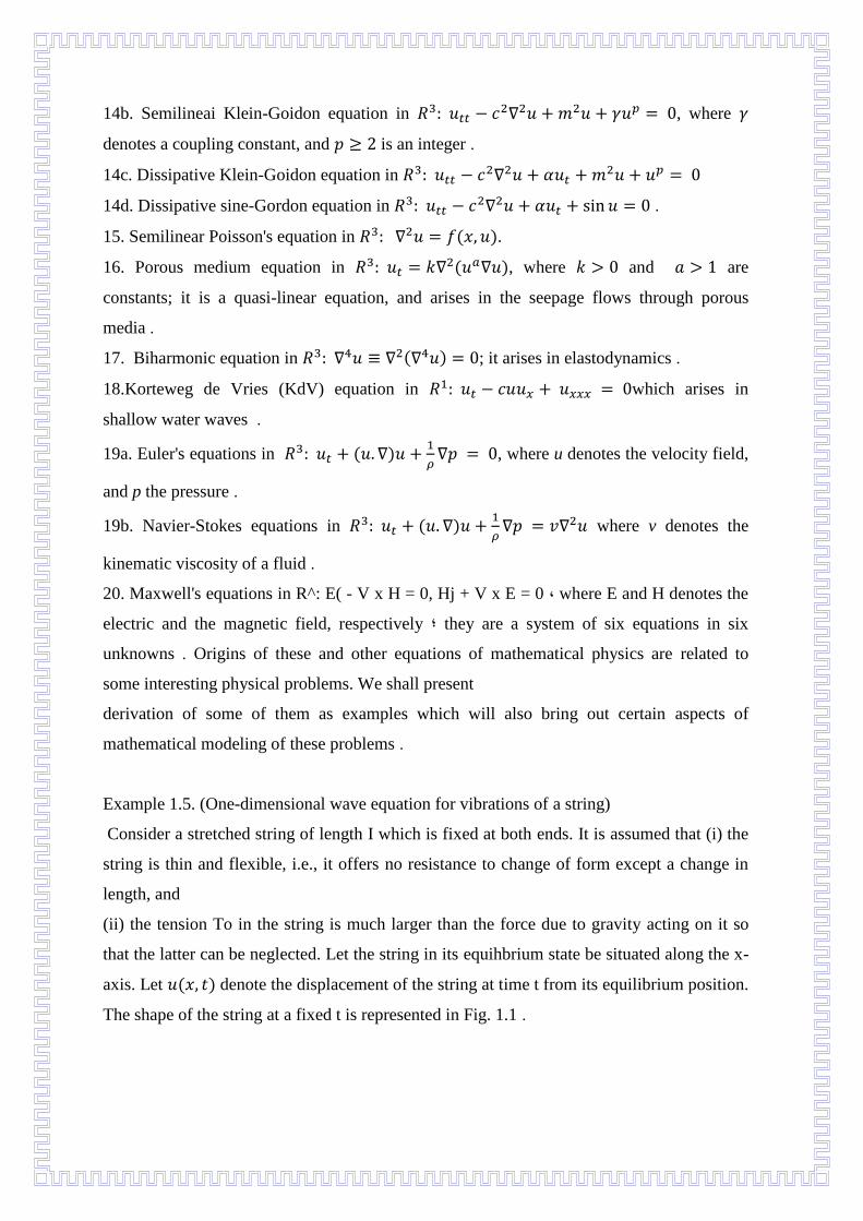
Example 1.5. (One-dimensional wave equation for vibrations of a string)

Consider a stretched string of length I which is fixed at both ends. It is assumed that (i) the

string is thin and flexible, i.e., it offers no resistance to change of form except a change in

length, and

(ii) the tension To in the string is much larger than the force due to gravity acting on it so

that the latter can be neglected. Let the string in its equihbrium state be situated along the x-

axis. Let ( ) denote the displacement of the string at time t from its equilibrium position.

The shape of the string at a fixed t is represented in Fig. 1.1 .

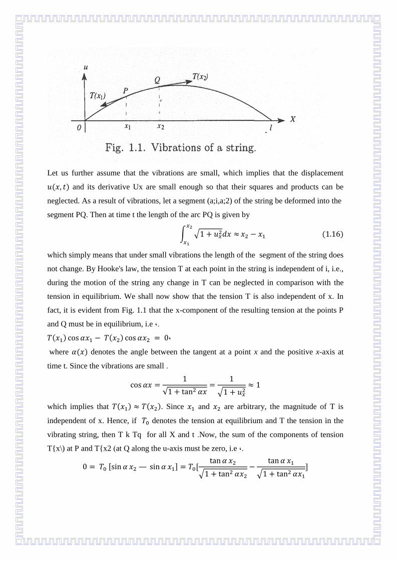
Let us further assume that the vibrations are small, which implies that the displacement

( ) and its derivative Ux are small enough so that their squares and products can be

neglected. As a result of vibrations, let a segment (a;i,a;2) of the string be deformed into the

segment PQ. Then at time t the length of the arc PQ is given by

∫ √

( )

which simply means that under small vibrations the length of the segment of the string does

not change. By Hooke's law, the tension T at each point in the string is independent of i, i.e.,

during the motion of the string any change in T can be neglected in comparison with the

tension in equilibrium. We shall now show that the tension T is also independent of x. In

fact, it is evident from Fig. 1.1 that the x-component of the resulting tension at the points P

and Q must be in equilibrium, i.e ,.

( ) ( ) ,

where ( ) denotes the angle between the tangent at a point x and the positive x-axis at

time t. Since the vibrations are small .

√

√

which implies that ( ) ( ). Since and are arbitrary, the magnitude of T is

independent of x. Hence, if denotes the tension at equilibrium and T the tension in the

vibrating string, then T k Tq for all X and t .Now, the sum of the components of tension

T{x\) at P and T{x2 )at Q along the u-axis must be zero, i.e ,.

[ ] [

√

√ ]

[

√

√

] [

] ( )

[

|

|

]

∫

using (1.16). Let ( ) denote the external force per unit mass acting on the string along

the u-axis. Then the component of ( ) acting OD the segment PQ along the u-axis is

given by

∫ ( )

( )

Let ( ) be the linear density of the string. Then the inertial force on the segment PQ is

∫ ( )

( )

Hence the sum of the components (1-17), (1.18), and (1.19) must be

zero, i.e.

∫ *

( ) ( )

+

( )

Since and are arbitrary, it follows from (1.20) that the integrand must be zero, which

gives

( ) ( )

( )

This represents the partial differential equation for the vibrations of the string .

If const, then (1.21) reduces to

( ) ( )

where √

( ) ( ) . In the absence of external forces, Eq (1.22) becomes

( )

which is the wave equation for free vibrations (oscillations) of the string.

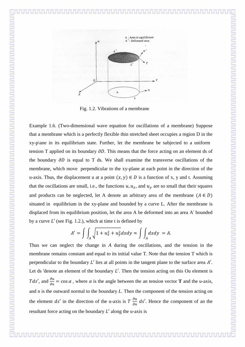
Fig. 1.2. Vibrations of a membrane

Example 1.6. (Two-dimensional wave equation for oscillations of a membrane) Suppose

that a membrane which is a perfectly flexible thin stretched sheet occupies a region D in the

xy-p\ane in its equilibrium state. Further, let the membrane be subjected to a uniform

tension T applied on its boundary . This means that the force acting on an element ds of

the boundary is equal to T ds. We shall examine the transverse oscillations of the

membrane, which move perpendicular to the xy-plane at each point in the direction of the

u-axis. Thus, the displacement u at a point ( ) is a function of x, y and t. Assuming

that the oscillations are small, i.e., the functions , and are so small that their squares

and products can be neglected, let A denote an arbitrary area of the membrane ( )

situated in equilibrium in the xy-plane and bounded by a curve L. After the membrane is

displaced from its equilibrium position, let the area A be deformed into an area A' bounded

by a curve (see Fig. 1.2.), which at time t is defined by

∫∫ √ ∫∫

Thus we can neglect the change in A during the oscillations, and the tension in the

membrane remains constant and equal to its initial value T. Note that the tension T which is

perpendicular to the boundary lies at all points in the tangent plane to the surface area .

Let ds 'denote an element of the boundary . Then the tension acting on this Ou element is

, and

, where is the angle between the an tension vector T and the u-axis,

and n is the outward normal to the boundary L. Then the component of the tension acting on

the element in the direction of the u-axis is

. Hence the component of an the

resultant force acting on the boundary along the u-axis is

∫

∫

∫∫ (

)

( )

by Green's identity, where, in view of small oscillations, we have taken , and

replaced by . Let ( ) denote an external force per unit area acting on the

membrane along the u-axis. Then the total force acting on the area A' is given by

∫∫ ( )

( )

Let ( ) be the surface density of the membrane. Then the inertial force at all times t is

∫∫ ( )

( )

Since the sum of the inertial force and the total force is equal and opposite to the resultant of

the tension on the boundary L', we find from (1.24)-(1.26) that

∫∫ * ( )

(

) ( )+

or, since A is arbitrary ,

( )

(

) ( ) ( )

This is the partial differential equation for small oscillations of a membrane. If the density p

= const, then Eq (1.27) in the absence of external forces reduces to

(

) √

( )

Example 1.7. (Heat transfer equation for a uniform isotropic body) Let ( ) denote

the temperature of a uniform isotropic body at a point ( ) and time t. If different parts

of the body are at different temperatures, then heat transfer takes place within the body.

Consider a small surface element of a surface drawn inside the body. Under the

assumption that the amount of heat passing through the element in time is

proportional to , , and the normal derivative

( )

where k is the thermal conductivity of the body which depends only on the coordinates {x,

y, z) of points in the body but is independent of the direction of the normal to the surface S,

and denotes the gradient in the direction of the outward normal to the surface element

. Let Q denote the ieat flux which is the amount of heat passing through

the unit surface area per unit time. Then Eq (1.29) implies that

( )

Now, consider an arbitrary volume V bounded by a smooth surface S. Then, in view of

(1.30), the amount of heat entering through the surface S in the time interval [ ] is

∫

∫∫ ( )

∫

∫∫∫ ( )

( )

by divergence theorem, where n is the inward normal to the surface S. Let denote a

volume element. The amount of heat required to change the temperature of this volume

element by in time is

[ ( ) ( )] ( ) ( )

where c{x,y,z) and p{x,y,z) are the specific heat and density of the body, respectively.

Integrating (1.31) we find that the amount of heat required to change the temperature of the

volume V by ( ) ( ) is given by

∫∫∫ ( ) ( )

∫

∫∫∫

( )

We shall now assume that the body contains heat sources, and let g{x, y, z, t) denote the

density of such heat sources. Then the amount of heat released by or absorbed in V in the

time interval [ ] is

∫

∫∫∫ ( )

( )

Since , we find from (1.31)-(1.34) that

∫

∫∫∫ [

( ) ( )]

or, since the volume V and the time interval [ ] are arbitrary ,

( ) ( )

(

)

(

)

(

) ( )

( )

which is the required heat transfer equation for a uniform isotropic body. If , and k are

constant, Eq (1.35) becomes

(

) ( ) ( )

where √

is known as the thermal diffusivity, and

denotes the heat source (sink) function. In the absence of heat sources )i.e., when g(x,y,z,t)

= 0 ), Eq (1.36) reduces to the homogeneous heat conduction equation

(

) ( )

In the case when the temperature distribution throughout the body reaches the steady state,

i.e., when the temperature becomes independent of time, Eq (1.37) reduces to the Laplace

equation

( )

For the derivation of the heat conduction equation in consider a laterally insulated

rod of uniform cross section with area A and constant density p, constant specific heat c,

and constant thermal conductivity k. We shall assume that the temperature u(x, t) is a

function

of X and t only, i > 0, and use the law of conservation of energy to derive the heat

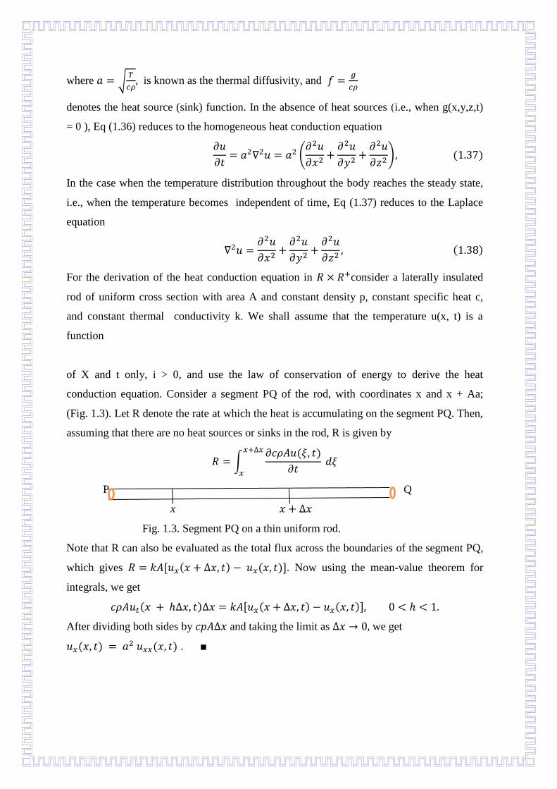
conduction equation. Consider a segment PQ of the rod, with coordinates x and x + Aa;

(Fig. 1.3). Let R denote the rate at which the heat is accumulating on the segment PQ. Then,

assuming that there are no heat sources or sinks in the rod, R is given by

∫ ( )

P Q

x

Fig. 1.3. Segment PQ on a thin uniform rod.

Note that R can also be evaluated as the total flux across the boundaries of the segment PQ,

which gives [ ( ) ( )]. Now using the mean-value theorem for

integrals, we get

( ) [ ( ) ( )]

After dividing both sides by and taking the limit as we get

( ) ( ) . ■

Example 1.8. {One-dimensional trafEc Bow problem) Let p{x,t )denote the traffic density

which represents the number of vehicles per mile at time t at an arbitrary yet fixed position

a; on a roadway. Let ^ a;, t) denote the traffic flow which is a measure of number of vehicles

per hour passing a fixed position x. Consider a section of the roadway bounded by the

positions a; = a;i and a; = a;2, and assume that there are no exits or entrances between these

two positions. Then the number A ''of vehicles in the segment [a;i, a;2] is given by N = p{x,

t) dt. The rate of change of A'^ with respect to time t is equal to the difference between the

number of vehicles per unit time entering the position at a; = a;i and that leaving at the

position , i.e ,.

∫ ( )

( ) ( )

As in the case of heat conduction (Example 1.7), Eq A-39), which is also known as the

integral representation of conservation of vehicles ,can be written as

( ) ( ) ∫

( )

∫ ( )

which after taking the partial derivative d/dt inside the last integral and noting that xi and

X2 are arbitrary leads to the required partial differential equation

( )

Let u{x,t) denote the velocity of a vehicle. Then, since the number of vehicles per hour

passing a given position is equal to the density of vehicles times the velocity of vehicles, we

obtain

* ) ( ) ( ).)

If we assume that the velocity u depends only on the density p, u = u{p), i.e., the vehicles

slow down as the traffic density increases, then

-- <0 . This inequality implies that the traffic flow depends only on

dp the traffic density, i.e., q = q{p), and Eq (1.40) then reduces to

Or

( )

( )

where ( ) . Eq (1.41) is a first order homogeneous quasi - linear partial

differential equation. ■

1.5. Superposition Principle

Let L denote a linear differential operator of any order and any kind .The superposition

principles for homogeneous and non-homogeneous linear differential equations are

represented by the following two theorems :

Theorem 1.2. Let Lu = 0 be a differential equation. Suppose and are two linearly

independent solutions. Then is also a solution .

Proof. By hypotheses . By definition ( ) ■

Theorem 1.3. If Lu = J2^Cifi be a non-homogeneous linear differential equation and if Lg^

= fk, then Yl^^iQi ** °' solution of the above differential equation .

PROOF. LYJlcigi = Yl'^CiLgt = YJl^ifi- Thus YX^idi satisfies the differential equation ■ .

It is obvious from these two principles that if f is a solution of an equation Lu = 0 and if F a

solution of Lu = f, then i; + F is also a solution of Lu = f. A generalized superposition

principle is defined as follows :

Theorem 1.4. If the functions Ui, i = 1,2,..., are separately the solutions of a linear

homogeneous differential equation L{u) = 0, then

00

the series u = 2_]CiUi is also a solution of the differential equation ,i=l

provided that the derivatives appearing in L{u) can be differentiated term-by-term .

Proof. In fact, if the derivatives of u appearing in L{u) — 0 can be differentiated term-by-

term, we have i=l

and since the equation L{u) = 0 is linear and a convergent series can be added term-by-term,

we can write

L{u) = L lY^CiuA =Y.CiL{ui)=Q .\ i=l / i=l

The sufficient condition for term-by-term differentiability is the uniform convergence of the

series

∑

Chapter 2

Method of Characteristics

It is customary in modern texts on partial differential equations either to completely ignore

first order partial differential equations or postpone their discussion to a much later chapter.

Since first order partial differential equations are important from both physical and

geometrical standpoints, their study is essential to understand the nature of solutions and

form a guide to the solutions of higher order partial differential equations .

First Order Equations

First order partial differential equations occur in a variety of situations. Some of the

common ones are traffic flow, conservation laws, Mainardi-Codazzi relations in differential

geometry, and shock waves. In order to solve first order linear, quasi-linear, or nonlinear

partial differential equations, the method of characteristics is very useful. This method is

explained in the next six sections .

Second order equations, confined to linear equations, are discussed in §2.7 .

We shall limit our discussion to problems in R?. An extension to higher dimensions, though

routine, is more complicated .

2.1 Linear Equations with Constant Coefficients

The most general form of first order linear partial differential equations with constant

coefficients is

aux + buy + ku = f{x,y). B.1 )

If u{x,y) is a solution of B.1) then

du = Uxdx + Uydy. B.2 )

Comparing B.1) and B.2) one gets the auxiliary system of equations

dx_ ^dy ^ du

a b f{x,y) — ku '

The solution of the left pair is bx — ay = c. The other pair

dx du

a f{x,y)~ku

can be reduced to an ordinary linear differential equation with u as the dependent variable

and a; as the independent variable. This equation is given by

du ku f{x, (bx — c)/a )dx a a '

the integrating factor for which is e ."/^^*This observation leads us to introduce a new

dependent variable

v = ue'^'^/", reducing (1.1) to av:c + bvy = fix, y)e''^/" = gix, y .)

Note that a reduction can also be obtained by substituting v = u e'^^^''. This substitution will

lead to av-c + bVy = f{x, y) ^^1^. Thus, we need to consider

only the formal reduced form

aux + buy = f{x,y). B.4 )

The auxiliary system of equations for Eq B.4) is

dx dy du a b f{x,y ')B.5 )dx du

The solution of — = -— is bx — ay = c, which when solved for x gives

a b ay + c , . . ^ , . , . dy du . ,,

X = —-—; a substitution of this value into — = -r- r yields

b b f[x,y )dy du b .fay + c

which reduces to du = F{y,c)dy. Its solution is u = G{y,c) + ci, where

Gy{y, c) = F{y, c). Thus, the general solution is obtained by replacing ci by

(j){c) and c by 6a; — ay, thereby yielding

u{x, y) = G{y, bx - ay) + (j){bx - ay .)

Eqs B.3) are known as the equations of the cha.racteristics. The system B.3) has two

independent equations, with two solutions of the form

F{x,y,u) = 0 and G{x,y,u) = 0. Each of these solutions represents a family of surfaces. The

curves of intersection of these two families of surfaces are known as the characteristics of

the partial differential equation .The projections of these curves in the (x, y)-plane are called

the base characteristics, which are often called characteristics for brevity when there is no

ambiguity. The general solution represents a family of surfaces, which are called integral

surfaces .Thus, the equation bx — ay = c represents a family of planes. The intersection of

any one of these planes with an integral surface is a curve whose projection in the (x, y)-

plane will again be given by bx — ay = c, but this time this equation represents a straight

line and is the base characteristic .The solution u on a base characteristic bx — ay = c is

therefore given by u = G(y, c) + ci, and the general solution is the same as above .

An alternate procedure is to introduce a new set of coordinates

= ^bx — ay, and r] = bx + ay. B.6 )

This substitution reduces Eq B.4) to

=,.F«,,), ^(£,,) = /((!L±i)Z|i!L^i)ZM ),,, .

and the solution of B.6) is

uitv) = m + G{tv), B.8 )

where G^(^, ??) = F{^,r]). If f{x,y) = 0 in Eq B.4), then the auxiliary system of equations is

dx/a = dy/b,du = 0. The solutions of these equations are bx — ay = c, and u = c-y = 4>{c) =

4>{bx — ay). This procedure can also be regarded as a problem in rotation of axes (see .)

Note that Eq B.8) is

u{x, y) = 4>{bx — ay) -\- G {bx — ay, bx + ay .)

If an initial condition u{x, tjj(x)) = ii{x) is prescribed, then

u {x, tp^x)) = iJ.{x) = (j){bx - ai}){x)) + G{hx - aip(x), bx + atpix ))

can be used to determine (j)(x) uniquely. Thus, the existence of a unique solution u for the

partial differential equation B.1) subject to the above initial condition is established. (For the

existence and uniqueness of the solution ,see end of §2.7 ).

Example 2.1. Consider

2Ux — iUy = COS X .

The auxiliary system of equations is

dx dy du cos a ;

The first solution is then given by 2,x + 2y = c. The other equation is

ddu du 1 — = . Its solution is u = Ci + - sinx. Noting that ci = /(c) and

2 cos a; 2 3 x + 2y = c, the general solution becomes

u = /Ca; + 2y) + - sin x .

Alternately, the substitution ^ = 3a; + 2y, 77 = 3a; — 2y reduces the equation to

1 i^ + V )

=""12'°'— '^

which yields

+ @/ = .isin(i .^±

On replacing ^ and 77 by their values in x and y, one gets the above general solution .

In this problem the characteristics are given by the curves of intersection of the planes 3a; +

2y = c and the integral surfaces u =- sina; + ci. The projections of these curves on the (a;,

y)-plane u = 0

are the base characteristics. Graphs of these characteristics are shown in Fig. 2.1 for c = 1

and Ci = 0 .characteristic plane 3 x+2 y - iiUi'iiial surface plane 3 x+2 y = 1

Fig. 2.1 .

If a linear partial differential equation is of the form P(x, y) Ux + Q{x,y)Uy = 0, then the

base characteristics and the characteristics are the same curves. We will now develop

solutions for some specific conditions prescribed on initial curves. For example, if u = 1 on

the initial curve y = 0, then

.1 . . /3 a; + 2y

u = 1 + - sm a; — sin

2 V 3

which is an integral surface denoted in Fig. 2.2 by S\. Also, if u = x ^on the initial curve y =

x, then

1 . Ca; + 2t/J 1 . 3a; + 2y

u = - sm a; H sin ,

2 25 2 5 '

which is another integral surface denoted by 82- The graphs of the integral surfaces Si and

S2 and the characteristics are shown in Fig .2.2 Note that an initial curve (or initial line) is a

curve where an initial condition on u is prescribed ■ .

I www I A complete Mathematica solution for this example and the

individual plots of the integral surfaces Si and 82 are available in the

Mathematica Notebook Example2.1 .ma .

It is obvious that the solution of a first order linear partial differential equation represents a

surface and contains an arbitrary function

and not an arbitrary constant. Clearly, the solution represents a family of surfaces. A unique

surface is obtained if u is prescribed on an initial curve, which is not a characteristic. The

reader can observe that the existence and uniqueness of the solution of a first order equation

are closely related to the existence and uniqueness of the solutions of the auxiliary system

B.5) of ordinary differential equations (see end of characteristics

Fig. 2.2 .

Example 2.2. Consider

The auxiliary system of equations is

dx dy du 1 x'^y

The first solution is then given by a;-4y = c, and the solution, following the method of the

previous example, is

M = Ci +2, x^ — Acx = ^'m +3 x'^ — Acx ^44 ■ ' ^ "44

On replacing c by a; - Ay, one gets the general solution

u = f{x- Ay) + ^~ ^^ = f{x -Ay )- — .^ +

2.2 Linear Equations with Variable Coefficients

The general form of first order linear partial differential equations with variable coefficients

is

P{x, y)u:c + Q{x, y)uy + fix, y)u = R{x, y). B.9 )

Once again our attempt is to eliminate the term in u from Eq B.9 .)This can be accomplished

by substituting where ^(x, y) satisfies the equation

P{x, y) ix{x, y) + Q{x, y) iy{x, y) = f{x, y ) .

Hence, Eq B.9) is formally reduced to

P{x,y)ux + Q{x,y)uy = R{x,y), B.10 )

where P, Q, R in B.10) are not the same as in B.9). The method for solving these equations,

known as Lagrange's method, is essentially the same as in the previous section except that

now the auxiliary system of equations is

dx _dy _du

P~Q'R ^^ '- ^^

which becomes more complicated. This system has two solutions of the type

g{x,y,u) = ci, and h{x,y,u)=C2 ,

representing two families of surfaces. The curves of intersection of these surfaces are called

characteristics of the equation. The projection of a in the plane u = 0 is called a base

characteristic .If R{x, y) = 0, then there is no difference in the base characteristics and the

characteristics. Frequently the word base is omitted from the term base characteristic. These

characteristics are clearly a one - parameter family of curves. In some cases it is convenient

to introduce a parameter, say s, in the auxiliary system of equations, which are then

expressed in the form

dx dy du

Example 2.3. Consider

Suj; + 4uy + 14(a; + y)u = 6x e .''^+^(~

The first step is to find a function C,{x,y) which satisfies the equation

Kx+Ky = l^{x + y .)

A particular solution of this equation is C,{x,y) = (a; + y)"^. Then the

substitution u = i;e~^^^'^' reduces the given equation to

3vx + 4Vy = 6a ,;

with auxiliary equations

dx dy dv Y ~ T ~ 6x 'A7* (ill dx dii )

The solution of -— = — is 4a; — 3w = ci, and solution of -— =-— 3 4 «1 '36 a ;

is f = X + C2. Now, as before, v can easily be found to be ti =

x^ + /Da; — 3y). Let us examine these solutions a little more. If we write ci = Ax — Sy =

g{x,y,v) and C2 = v — x^ = h{x,y,v), and consider an expression of the form F{g, h) = 0,

then

Fx = Fg{gx + gvVx) + Fh{h:^ + Kv^) = 0 ,

which reduces to

4F3 + (i;^ - 2x)Fh = 0 .

Similarly the expression for Fy yields

-3 Fg +VyFh = 0 .

Eliminating Fg and Fh from these two equations, one gets

4 Vx -2x det - Vy 0 , I.e ,.3 vx + iVy = 6x .

Thus, F{g, h) = 0 is also a solution of the differential equation. Of course, we have to

replace v hy u 6^^+^^ to obtain the solution of the original problem ■ .

Solutions of the type F{g, h) = 0 or g = F{h) or /i = F{g) are known as general solutions .

Definition 2.1. Two C^ functions g and h are said to be func - tiona.lly independent if Vg x

V/i ^ 0 .

We shall state an important theorem .

Theorem 2.1. Let g = ci and h = C2 be any two functionally independent solutions of Eq

B.9). Then g = F{h), or h — F{g), or

F{g,h) = 0 represents the general solution of Eq B.9 .)

Corollary 2.1. If g = ci is a solution of Eq B.9), then F{g) = 0

is also a solution of Eq B.9 .)

Example 2.4. Let us further consider the reduced equation 3vx +

4Vy = 6x from Example 2.3. The auxiliary equations in the parametric form are

dx dy dv The solutions are

X = 3s -\-ci, and y = As + C2, B-13 )

and, therefore ,

V = Qs"^ + 6cis + C3. B.14 )dv

The last solution is obtained by first substituting x = 3s+Ci in — = ds.x

The values of x, y, v in terms of s represent the parametric form of the equation of the

characteristics of the given partial differential equation .In order to find a specific

characteristic, we need to have an initial condition, e.g., x = Xq, y = yo, v = Vq at s = Sq. By

eliminating s from B.13) and B.14) we get

4a; — 3y = 4ci — 3c2 = a and v = x^ — c^ + C3 = x"^ + C ,from which we get

V = x"^ + f{4:X - 3y).u

We note here that, except for singular cases, a unique characteristic will, in general, pass

through a point in space. Thus, if a continuous initial curve is prescribed, then a unique

characteristic will pass through every point of the initial curve. The locus of these

characteristics will form the integral surface. Hence, if the initial curve is a characteristic

itself, then the existence of an integral surface cannot be guaranteed see end of §2.7 .)

Example 2.5. Consider

u^ + e^Uj/ = y, u{0,y) = l+y .

The auxiliary system of equations is

dx dy du 1 e^ y ' B.15 )

Thus, the solutions of the auxiliary system are given by dy = e^ dx ,which yields y = e^ + c.

From the second set of Eq B.15) one gets du = y dx which results in du = (e^ + c)dx. Its

solution is u = e^ -\-ex + ci ,hence

u-= e" +CX + f{c), or u = e^ + (y - e^)a; +/(y - e .)""

Now, in view of the initial condition, u{0,y) = 1 + /(y — 1) = 1 + y ,which yields /(y) = y +

1. Hence the solution is

u{x, y) = e^ + (y - e^)x + y-e^ + l = l+y + xy- xe ■ .^

I www I The plots of the surfaces y = e^ + c and u = e^ -\- {y — e^) x for c = 1 are available

in the Mathematica Notebook Example2.5.ma .The intersection of these surfaces is a

characteristic .

Example 2.6. Consider

2yUx + Uy=x, u@,y) = /(y .)

The auxiliary system of equations is

dx dy du

2y ~ T ~ T '

In this example, a slightly different procedure will be demonstrated. We will first find the

equation of the characteristics through an arbitrary point {xo,yo) on the integral surface. The

left pair in the auxiliary equations is dx = 2y dy, whose solution is the family of surfaces

Si : X = y'^ +c .When a surface Si passes through the point {xo,yo), its equation

becomes x = y^ + Xq — yo- If the initial curve is a; = 0, where

u@, y) = /(y), then the value of y on the initial curve is given by

yp = y^—xo, where yo is the value of y on the integral surface through ( a;o,yo) at a; = 0.

The right pair of auxiliary equations is du = xdy ,which also represents a family of surfaces.

Let us denote the integral surface through @, yo) by 82- The curve of intersection of Si and

52 is a characteristic. The differential equation of this characteristic is given

by du = {y^ + Xq — y^)dy. Its solution is u = — + {xq -yo)y + ci .

At a; = 0 ,w@, yo) = -J + {xo - yl) yo + ci = /(yo ,)

and substituting the value of yo, one gets

c. = f{{yl-x,f") + l{yl-x,fl \

Using this value of ci in u, the value of u at {xq, yo) is given by

u{xo, yo) = ^{yl- xof'^ - -yl + xoyo + /((yo " x^f .)^'

Since {xo,yo) is an arbitrary point, the expression for u(a;o,yo) is generalized to

u{x, y) = \{y^- xf' - ly' + xy + f{{y' - xfl \ ^ .

Example 2.7. Consider

(a; + 2y)ux + (y - x)Uy = y .The auxiliary equations are

dx dy dv x + 2y y-x y '

The first two equations can be expressed as

dy_ ^ y-x dx X + 2y '

This is a homogeneous ordinary differential equation of the first order .A standard

substitution for such problems is y = vx, which leads to a first order ordinary differential

equation with separable variables

A + 2v)dv _ dx _1 +2 i;2 ~~ x '

This equation can be solved to give

v/2tan-i — + ln(a;2 + 2y^) = cj .X

The other solution can be obtained by observing that dx + dy = 2>du ,

thus yielding u = —{x -\-y) -\- C2. Hence the general solution becomes

u='^{x + y)+f [^2 tan-i ^ + ln(a;2 + 2 . .])^^

I www I The plots of the surfaces

\/2 tan~^ ^^+ln(a;^ + 2y^) = 1, and u=-{x + y )X 3

are available in the Mathematica Notebook Example2.7.ma. Note that

the intersection of these two surfaces gives a particular characteristic .

2.3 First Order Quasi—linear Equations

If the coefficients P, Q, and R in Eq B.9) are functions of x, y, and u ,but not of Ux and Uy,

then the equation is known as quasi-linear. In these equations the first order derivatives

occur only in the first degree ,although the equation need not be linear in u. Such equations

occur in shock waves of various kinds, e.g. traffic flow, water waves. The basic

technique is the same as for first order linear equations. The starting point is still the system

of auxiliary equations B.11 .)

Example 2.8. Consider the quasi-linear equation

Ux+uuy = 0, u@,y) = f(y .)

The system of auxiliary equations is

dx dy — =— , du = 0 .1 u QiX dv

Here du = 0 implies u = c. Using this value of u in — = — one gets 1 u y = ex + Ci. Thus,

the characteristics are given by the curves of intersection of the surfaces y — ux — Ci and

u = c, and the general solution can be expressed as u = g{y — ux). Applying the initial

condition, we get f{y) = 9{y)- Hence the solution to the problem \s u — f{y — ux .)

y If f{y) = y^ the solution becomes u . =

If /(y) = y^) then we have u = (y — ux)'^, which after some algebraic simplification yields

l + 2xy± JT+lxy = "2^^

A careful examination by checking the limit as x —^ 0 shows that the valid solution is

1 +2 xy - yT+5y u =2 a;2

I www I In the Mathematica Notebook Example2.8.ma, the following plots are given :

(i) The graphs oi y — ex = Ci for c = 1,2,3, and ci = 0,1,2. These

curves are characteristics and also base characteristics .y

(ii) The graph oi u = represents an integral surface ^ , ,^ ,..., .1 +2 a;y - A/rT4iy

(ui) The graph of u = —^ represents another mtegral surface .

Example 2.9. Consider

U:c+9iu)Uy = 0, u{0,y) = f{y .)

The system of auxiliary equations is

dx dy 9{ uy du = 0 .

As in Example 2.7, u = c, and y = g{c)x + ci. The general solution is

u = h{y — xg{u)). After applying the initial condition, we get /(y = )

h(y). Hence the solution to the problem is u = /(y — xg ■ .))^{

Example 2.10. Consider

u^-\-Uy = u'^ + l, u{0,y)=f{y .)

The auxiliary equations are then

du dx = dy 1*2 4.1 '

The solutions are y = x + c, and tan~^ u = x -\- Ci. Thus, the general solution is u = tan(a; +

g{y — x)), and the particular solution for the problem is tana; + /(y - x )

u = -. r — ■ . I — J\y ~ x) tana ;u=y characteristic Parabolic cylinder

X = y ^Fig. 2.3 .

Example 2.11. Consider the partial differential equation

2yUx +Uy = 1 ,

where u = 1 is prescribed on the initial curve 2/ = 0 (a;-axis) for 0 < a; < 1. The auxiliary

system B.11) for this partial differential equation is

— = dy = du .2 y

The solution of dx = 2y dy is the parabolic cylinder x = y'^ + A, while that of du = dy is the

plane u = y + B, where the parameters A and B are constant for each characteristic. For any

point {xo,yo,Uo) we find that A = Xo — yQ, and B = zq — yo- If the point {xo,yo,Uo) is

taken ,e.g., as the origin of the the coordinate system, then

X — y^, and u = y. B.16 )

The equation of the characteristic is the intersecting curve (in this case ,the parabola) of the

solution B.16), as shown in Fig. 2.3 .The characteristic through the point A,0,1) is the

intersection of the parabolic cylinder x = y'^ + 1 and the plane u = y + 1. Moreover ,

ii u = x"^ on the initial curve y = 0, then u = y + {x — y^Y represents

the integral surface ■ .

Example 2.12. Consider

Ux + lUUy = 1 .The auxiliary equations are

dx = -— = du .2 u

The solutions are u = x + c, and u^ = y + ci. Hence the general solution is

u = a; +/(u^ - y), or u^ =y + g{u- x .)

It is important to choose the appropriate general solutions for the given initial conditions.

Thus, for example, if the initial line (curve )is a; = y, and the value of u on this initial line is

u{y,y) = y, then from the first solution we get u = x. But the second solution gives

y^ = y + 5@), which does not yield a value for the function g .If the initial line is y = a;, and

u{y, y) = y^, then the second solution yields

u'^ =y + (u-x)'^ + 2{u -x)±{u- x)^/^+A{u ,^^

where the plus sign corresponds to a; > -, y > -, and the minus sign to a; < -, y < -.

Substituting y = a; and u = y^ in the second solution ,we have y^ = y + g(y'^ — y). Now let

z = y'^ — y, then

y = - A ± Vl + 4^) , and y* -y = z'^ + 2z± zVl + 4z = g{z .)

which gives the solution of the equation. But if we use the first solution we get y^ = y +

f{y'^ — y), which is more difficult to resolve ■ .

Example 2.13. Consider

{y + u)u:, + yuy = x-y .

For this problem, it is convenient to use the auxiliary equations in parametric form B.12),

i.e ,.

dx dy du y+u y x-y

which can be rewritten as

dx dy du as as as

The solution of the middle equation is y = Ae". Addition of the first and third equations

yields

d(u + x )-^- j =u + x .ds

Its solution is u + X = Be". Subtracting the first equation from the third results in

d(u — x )- L^ ^ =x-u-2y ,ds ^

which can be expressed as

d(u - x )-{ + ^ u-x) = -2Ae ^ds

This equation is linear in u — a;. Its solution is

u- X = Ce^" - Ae \ y

Replacing e* by — in the two solutions, we get

B ^ CA u + x=—y, and u — x + y . = A y

Noting that B/A and CA can be replaced by ci and C2, and that

C2 = f{ci), we have { u-x + y)y = f(^^^ B.17 )

as the general solution of the given equation ■ .

Example 2.14. Consider

xyuux + {x'^ — u^)uy = x^y .

The auxiliary equations are

dx dy du xyu x-^ — V? x'^y

From

dx du xyu x'^y '

we get X — u^ = ci, and then using this solution in

dy du x-^ — w^ x-^y

we obtain

cidu y°-y =-^-:— • u^ + ci

This equation yields u ' la tan ' y 1 ^ r 9 2 a tan —I-C2, if ci = a , a

■- r <^2, 11 ui — u

u — a aln——-+C2, ifci = —a .^u + a

The general solution can now be found .

2.4. First Order Nonlinear Equations

The general form of a first order nonlinear equation is

F{x, y, u, u^, Uy) = 0. B.18 )Consider the two-parameter family of surfaces

f{x,y,u,a,h)=0. B.19 )

Then

fx + fuUx = 0, and fy + fuUy = 0. B.20 )

Equations B.19) and B.20) form a set of three equations in the two parameters a and b. If a

and b are eliminated from these equations ,one gets an equation of the type B.18).

Therefore, it is reasonable to assume that the solution of B.18) is of type B.19). It is clear

that any envelope* of this family will also be a solution of equation B.18). At

this point we state the Cauchy problem: Determine u{x, y) such that u and its partial

derivatives satisfy

F{x,y,u,Ux,Uy) =0 ,

subject to the condition u{0,y) = 4>{y). In this case u{x,y) is prescribed on the initial line a;

= 0 (y-axis). Initial data can, however ,be prescribed on any simple curve which is not a

characteristic of Eq B.18). Thus, for example, if the parametric form of the curve

is a; = x{s),y = y{s), then the initial data can be written as

u(a;(s),y(s)) =^{s .)

We will now distinguish between different kinds of solutions of equation

B.18 .)Complete integr&l: A two-parameter family of solutions of the type

f{x, y, u, a,b) = 0 is known as a complete integral .General integral: If 6 = g{a), where g is

an arbitrary function and an envelope of the family of solutions of the complete integral is

found ,then the envelope whose equation contains an arbitrary function is known as the

general integral corresponding to the solution B.19 .)Singular integral: If the two-parameter

family of solutions B.19 )has an envelope, then the equation of this envelope is known as

the singular integral of B.18 .)Cauchy's method of characteristics: This method is similar

to the method of characteristics discussed earlier for linear and quasi - linear partial

differential equations .Consider a first order nonlinear equation B.18). For convenience ,

we will use the notation

Ux = p and Uy = q. B.21 )

*An envelope of the family of surfaces /(x, y, u, a, b) is a surface which touches

some member of this family at every point .

If u(x,y) = c is a solution of B.18), then u and its partial derivatives satisfy the equation

B.18). But the total derivative of u is given by

du = pdx + qdy. B.22 )

Differentiating B.18) and B.22) with respect to p, we get

dx + ^dy = 0, B.23 )dp

and

Fp + F,| = 0. B.24 )

Equations B.23) and B.24) yield

dx_ ^dy_ ^ pdx + qdy ^ du ^^ ^ Fp Fg pFp+qFg pFp+qFg

These are the characteristic (or auxiliary) equations of Eq B.18). It can be easily verified

that they reduce to the characteristic equations of

a linear or a quasi-linear partial differential equation according as Eq B.18) is linear or

quasi-linear. The parameter t introduced in B.25) is

such that

= |f,. I^F, and '^=VF,*,F,. B.26 )

Since p is a function of t, it follows that

dt) ddu dv Differentiating Eq B.18) with respect to x, we have

Fx + FuUx + FpPx + Fgqx = 0 .

Using this equation and inserting the value of Fpp^ + Fgqx in B.27 ,)we get

= ^-{ Fx + FuUx) = -{Fx +pFu). B.28 )

Similarly ,

= ^-{ Fy+qF^). B.29 )

Combining equations B.25), B.28), and B.29) we get

dx dy du dp dq

Fp Fg pFp + qFg -{Fx+pFu) -{Fy+qF )^

dt. B.30 )

This system of auxiliary equations (also known as the characteristic equations) is used to

solve a nonlinear equation by Cauchy's method .The difference between the equations B.25)

and the corresponding equations B.11) for a linear partial differential equation is that the

equations B.25) contain p and q explicitly and, therefore, in order to solve them we need

additional equations which are included in B.30 .)The solution is found by eliminating p and

q from the solutions of B.30) and the given equation. The eliminant will, in general, contain

two arbitrary constants and will represent a complete integral of the equation. We

demonstrate the method by the following examples .

Example 2.15. Consider

u = 4pq .

The auxiliary system B.30) for this equation is

dx , dy ^ du ^ dp dq B.31 )

Since we get

dx dq , dy dp --=4-- , and --=4 -- , dt dt dt dt x + ci= ^q and y + C2 = 4p. B.32 )

Substituting these values of p and q into the given equation, we get the

complete solution as

u=-(a; + Ci)(y + C2). B.33 )

However, if we demand that the solution pass through a given curve ,then B.33) may or

may not yield the required solution. For example ,since the solution of

d'^x dq dx ' d^ ~~ 'di~ ^~ ~~di

is a; = ci + C2 e~*, we can require that u = y^ be the initial condition on the initial curve a;

= 0, which corresponds to t = 0. Then the solution given by B.33) fails to yield the required

solution. To avoid this situation we follow an alternate approach. The initial values for

X, y, and u can be taken to be Xq — 0, Vo = ^i and Uq = v^, where v is — I . Thus ,

9yJo fdu \ y

and since Uq = 4po9o, we find that the initial value of p is po = -r- But from equations

B.31) we note that p and q can be solved in terms of t as

V = Ae-\ and q = Be-*. B.34 )Substituting the initial values in B.32) and B.34) we find that

ci = 8^, C2 = -J//2, A = y/8, B = 2v .

Then, from B.32) and the given equation, x, y and u can be expressed in terms of ly and t as

x = 8iy{e-*-l), y=^(e-* + l), u = iyh-^K B.35 )

The required solution can now be found by eliminating v and t fromB.35 as

ivG+^y

I www I In the Mathematica Notebook Example2.15 .ma, the plot of the above solution

represents an integral surface .We will now consider some special cases of equation B.18 .)

Example 2.16. Consider

u=px-\-qy + f{p,q), or F = px + qy + f{p,q) - u = 0. B.36 )

This is a special type of nonlinear equation. It always has a complete solution which can be

obtained in a simple manner. The last two of the characteristic equations are

dp = 0, and dq = 0 ,which yield p = a and q = b, where a and b are arbitrary constants .

Substituting these values in B.36), one gets u = ax + by + f{a, b) as the complete solution.

Equations of the type B.36) are known as Ciairaut equations. There are other special types

of partial differential equations which yield the complete solution in a relatively easy

manner ■ .

Example 2.17. Consider

f{p,q)=0. B.37 )

Note that the characteristic equations will yield dp = 0 and dq = 0. So p = a, and solving f{p,

q) = 0 for q will give q = g{a); then observing that

du = adx + g{a) dy ,

we get

u = ax + g{a)y + c .

As an example, let /(p, q) = p'^ + q^ — 1 = 0. The auxiliary equations

B.30) are dx dv —- = p —-= q^ du = dt, dp = 0, dq = 0 .at dt

Using dp — 0, we get p = a and q = \/l — a'^, and these two combined with du = pdx + qdy

yield

u = ax + yyl — a'^ + c .

This is a complete solution. Another complete solution can be obtained

dx

by using p = a in —- = p and noting that du = dt, thus getting

dt dx du = —, which gives

a X u = —\- a .a du

Similarly, du = —j== implies that V1 - a ^U=-j^=^fi .

Thus, we can write au = x + aa, and

u^/l - a^ = y + aC .

Replacing aa and a/? by -c and -d, respectively, and eliminating a we get

U^ = ix- CJ + {y- df ,

which is another complete solution ■ .

Example 2.18. Consider

Fiu,p,q)=0. B.38 )

The last three terms of the system B.30) yield

dp dq , dp dq

dt, or

-pFu ~qK p q

i.e., p = a?q, where a? is an arbitrary constant. This equation together

with B.38) can be solved for p and q, and then we proceed as in the

previous example. Thus, let F{u,p, q) = v?+pq—A = 0. Then following

the above procedure we have p = a?q, which gives

9 ± =-\/4 — w^ and p = ±a\/4 — w ^a

Therefore, since du = p dx + q dy, we have

or

which gives

Hence

du = ± v 4 — u^ f a da; H— dy \ -(±^^^ adx + ldyy ■-1 . " f 1 ^ sm — — ± [ ax -\— y + c . ]

2 \ a J u = ±2 sin ( a a; H— y + c] . i

I www I In the Mathematica Notebook Example2.18 .ma, the plots of

u = 2sin(aa;H— y + c

for c = 0,1, 2, and a = 1,2 represent some particular integral surfaces .

Example 2.19. If F{x,y,u,p,q) = 0 is independent of u and can be expressed as 4'{x,p) =

ip{y,q), then each of these functions must be constant.Thus, if (p{x,p) = c and tpiy, q) = c

can be solved for p and q ,then a complete integral can be obtained. For example, consider

F{x,y,u,p,q)=p^{l-x'')-q\A~y^)=0 .

Then which gives

P p\l-x :'a Vl-x ^and q ■

x/4^7 'where we have ignored the negative solutions. Now since du = pdx + qdy, we have

du = . ax H j=^ dy ,V1 — x'^ -y'4 — y ^

which can be integrated to give

u = a ( sin~^ x + sin~^ - j + 6 ■ .

I www I In the Mathematica Notebook Example2.19.ma, the plots of the above solution for

a = 1 and 6 = 0,1 represent some particular integral surfaces .

Example 2.20. Consider

F{x,y,u,p,q) = 2pqy - pu - 2a = 0, B.39 )

for which

Fj; = 0, Fy = 2pq, Fu = -p, Fp = 2qy - u, and F, = 2py .

The auxiliary equations are

dx dy du du dp dq 2 qy — u 2py 2pqy — pu + 2pqy pu + 4a p^ —pq

The last pair reduces to

dp dq

— +— =0 ,

p q

which gives pq = a. Using this value of pq in B.39), we get

2ay — pu — 2a = 0 ,

which yields pu — 2ay — 2a, and q y-a ')

These equations after integration yield

u^ = 4(aj/ — a)(x — /3 ■ .)

2.5. Geometrical Considerations

Before we discuss the geometrical interpretation of the partial differential equation B.18),

i.e., F{x,y,u,p,q) = 0, let us recall the geometrical interpretation of a first order ordinary

differential equation

y' = f{x,y). Here f{x,y) represents the slope of any integral curve at the point {x,y). This

slope is unique at every point. If we graph f{x,y) = c, then the curve so obtained is known as

an isocline or a curve of constant slope. Of course, the curve itself does not have constant

slope, but every integral curve which intersects f{x,y) = c has the slope c at the point of

intersection. Since the correspondence between integral curves and the points of an isocline

is one-to-one, the number of integral curves is, in general, equal to the number of points

on the isocline, i.e., there exists a single infinity of them. However ,the exception to this rule

occurs when isoclines intersect at a point, in which case the point is a singular point of the

differential equation, or when the isocline is also a solution curve, in which case the isocline

is a straight line with slope c and the isocline is an envelope of the integral

dv V curves, except for the equation -^ = — whose isoclines and the integral

ax X curves are the same .The situation for a partial differential equation is somewhat

complicated. In this case the values of p and q are not unique at a fixed point {x,y,u). If an

integral surface is g{x,y,u) = 0, then p and q represent the slopes of the curves of

intersection of the surface with the planes u = const. Moreover, p, q, —1 represent the

direction ratios of the normal to the surface at the point {x,y,u). The derivatives p and

q are constrained by Eq B.18). Obviously, at a fixed point, p and q can be represented by a

single parameter. Hence, there are infinitely many possible normals and consequently

infinitely many integral surfaces passing through any fixed point. So, unlike the case of

ordinary differential equations, we cannot determine a unique integral surface by making it

pass through a point .

Cauchy established that a unique integral surface can be obtained by making it pass through

a continuous twisted space curve, also known as an initial curve, except when the curve is a

characteristic of the differential equation. Now, the infinity of normals passing through a

fixed point generates a cone known as the normal cone. The corresponding tangent planes

to the integral surfaces envelope a cone known as the Monge cone. In the case of a linear

equation, the normal cone degenerates into a plane since each normal is perpendicular to a

fixed line .Consider the equation ap + bq = c. Then the direction p,q,—l is perpendicular to

the direction ratios a, b, c. This direction is fixed at a fixed point. The Monge cone then

degenerates into a coaxial set of planes known as the Monge pencil. The common axis of

the planes is the line through the fixed point with direction ratios a, b, c. This line is known

as the Monge axis .

2.6. Some Theorems on Characteristics

Suppose u{x,y) = f{x,y) is an integral surface S of the partial differential equation Eq B.18).

Then the set of numbers

\xo,yo,uo=u{xo,yo),Po = i^-] - 9o ( =- ) ^

which represents a plane with normal (po,9o, — 1) and passing through the point {xq,

yo,Uo), is called a piane element. If the point {xq, yo,Uo )lies on S, then the element

{xo,yo,Uo,Po,qo) satisfies Eq B.18) and is called an integra.1 element of the surface. Let il

be a neighborhood of ( o,yo) in the plane u = 0. If the functions f^; and fy are continuous

in R, then the element ixo,yo,Uo,po,qo) is called a tangent element of S .

A curve F with parametric equations x = x{t),y = y{t),u = u{t )lies on the surface S if u{t) =

f{x{t),y{t)) for all admissible values of t .If a point Po on F corresponds to the value to of

the parameter t, then the direction of the tangent line is given by ( -r-, -^, -;- 1 . This

\dt' dV dt ^^^, )

direction is normal to I po = (^)to.9o = (^)toi -1 " ) iu\ (dx\ (iu \

Thus, a set of five functions x{t),y{t),u{t),p{t),q(t), which satisfy the condition

du , ^ dx , , dy Tt='^'^Tt^'^'^it ^

defines a strip on the curve F. If this strip is an integral element, then it is an integral strip of

the partial differential equation. If this integral strip at each point touches a generator of the

Monge cone, then the integral strip is a characteristic strip .We will state some theorems on

the characteristics. The proofs can be found in the references cited below .

Theorem 2.2. A necessary and sufficient condition for a surface to be an integral surface of

a partial differential equation is that at each point its tangent element should touch its

elementary cone (tangent cone or Monge cone) of the equation .

Theorem 2.3. The function F{x, y, u,p, q) is constant along every characteristic strip of the

equation F{x,y,u,p,q) = 0 .

Theorem 2.4. If a characteristic strip contains at least one integral element of F{x,y,u,p,q)

— 0, it is an integral of the equation F{x,y,u,Ux,Uy) =0 .For the linear partial differential

equation ap + bq = c, we have

Theorem 2.5. Every surface generated by a one-parameter family of characteristic curves is

an integral surface of the partial differential equation .

Theorem 2.6. Every characteristic curve which has one point in common with an integral

surface lies entirely on the integral surface .

Theorem 2.7. Every integral surface is generated by a one-paramet family of characteristic

curves .

Theorem 2.8. If dx dy dy dx dy <dx ds dt ds dt dt dt

everywhere on an initial curve C, then the initial value problem has one and only one

solution. If, however, D = 0 everywhere along C ,the initial value problem cannot be solved

unless C is a characteristic curve, and then the problem has an infinity of solutions .

Proofs of Theorems 2.2, 2.3 and 2.4 can be found in Sneddon A957 ,

pages 62-64), and of Theorems 2.5, 2.6, 2.7, and 2.8 in Courant and

Hilbert A965, pages 64-66 .)

Second Order Equations

2.7. Linear and Quasi linear Equations

For a linear or quasi-linear partial differential equation of second or higher order, the

characteristic equation is determined by the highest order terms in the partial differential

equation. These terms are known as the principal part of the partial differential equation.

While the solution of the characteristic equation leads to the solution of the

first order partial differential equation, the solution of the characteristic equation of a

second order partial differential equation leads to a coordinate transformation which when

applied reduces the second order partial differential equation to a simpler form. This

simpler form is called the canonicaJ form. Consider a second order partial differential

equation

ail Uxx + 2ai2 Uxy + 022 Uyy -\- F{x, y, u, Ux, Uy) = 0, B.40 )where an, ai2 and 022 are

functions of 2; and y only, and F is a function of X, y, u, Ux, and Uy. The different

canonical forms of Eq B.40) are

Elliptic : U{{ + u^^ + G{^,rj,u,u^,Uj,) = 0 ,

Hyperbolic , f H, - u,, + G{^,,,u,u,,u,) = 0 ^^^ ^^ ,

[u^^ + G{^,r],u,u^,u ,)^

Parabolic : u^j + G{^, rj, u, u^, u^) = 0 .

In order to reduce Eq B.40) to a canonical form, we introduce a reversible transformation

{^ = ^x,y), and r]^r]{x,y), B.42 )

with the condition that the Jacobian

^-=^||| exr?,-r?,ex7^0. B.43 )

Using this transformation and noting that

Ux = u^£,x +u^r}x ,

Uy = U(^iy + Ur,r]y ,

Uxx = U^i ^l + 2U{^ ^x Vx + Ur^-n Vl + H ^xx + Ur, Vxx ,

Uxy = U^i ix ^y + Mfr, {L Vy + ^y Vx + )

Uyy = UjJ il + 2Uj^ iy TJy + U^^ 7?^ + Uj ^yy + U^ r]yy ,

B.44 )

Eq B.40) reduces to

^11 Uff + 2^12 Uf^ + A22 Ur,r, + G{^, T], U, Uf, W,,) = 0, B.45 )

where G is a function of ^,ry,u, uj, and u^, and ^n, A12, and A22 are functions of ^ and rj,

given by

^11 = an £,1 + 2ai2 £x £y + a.22 Cy ,

A\2 = an ix Vy + ai2 {ix iy + iy Vx) + 0.22 £y Vy^ B.46 )

A22 = an T]l + 2ai2 Vx Vy + 0-22 "nl -

The function G is linear or nonlinear according as F is linear or nonlinear .

If we now choose ^ and r] such that both satisfy the condition

aiiex + '^ai2£x£y+022^1 = Q, B.47 )

then ^11 = A22 = 0. Eq B.40) will then reduce to 2^12 u^r, + G{^, r], u, u^,Ur,) = 0 .

It can be verified (after some tedious algebra) that

^u-^11^22= {aJ2^ 0,110.22) {^xVy+^vVx) ■ B.48 )

This means that the sign of the quantity (ai2 "^11^22) is invariant under the reversible

transformation B.42), and the quantity itself is invariant if I J| = 1. An important

consequence of this result is that the partial differential equation does not change its

classification under nonsingular transformations [see §1.3, where it was proved that if C =

4'{^^y) is a solution of Eq B.47), then (f){x,y) = c is a solution of Eq A.10)]. Both

equations A.10) and B.47) are called characteristic equations of the partial differential

equation B.40). Equation A.10) has two solutions given by

^ ^ai2 ± \/a\2 - ^11^22 ^2 ^gN dx 2ai2

If the partial differential equation is hyperbolic, then there are two solutions, resulting in

two characteristics for the partial differential equation. If the partial differential equation is

parabolic, then there is only one real solution, and hence only one characteristic. In the

elliptic case there are no real solutions, and so there are no characteristics .In order to

transform the partial differential equation to its canonical form, we introduce two

independent variables ^ = ^{x,y) and

T] = r]{x,y), where ^ and rj are solutions of Eq B.49). In the case of a parabolic equation we

have only one solution, so rj is chosen arbitrarily except that it must satisfy the condition

B.43). In the case of an elliptic equation, the solutions are complex conjugates, and we

can use the real and imaginary parts of the solutions as the new independent variables. It

will be shown in Chapter 5 that canonical forms are frequently necessary to solve partial

differential equations by the method of separation of variables .We will now demonstrate

the effectiveness of this technique for reducing second order partial differential equations to

canonical forms by some examples .

Example 2.21. Transform the partial differential equation

y^ UXX - 4:Xy Uxy + AX"^ Uyy + (X^ + 2/^) Ux +Uy =0

to its canonical form. This equation is parabolic and its characteristic equation, given by

y^ [dyf +Axydxdy + ix^ {dxf = 0 ,has only one solution

dy 2x ,.,.,, „ 2 2 -;— , = which yields 2x +y = c .dx y

In this case there is only one characteristic curve, and so we make the substitution

= ,£2 x'^-\-y^, and r] = x .

The substitution for rj is arbitrary in this situation, the only condition being that the Jacobian

should be nonsingular. Thus, we have

Uy = 2yui ,

Uxx = 162;'^ U{{ + 82; Uf,, + Urj-q + 4Uj ,

Uxy = 8x y u^^ + 2y u ,^^

Uyy = 42/^UjJ + 2U .{

Substitution of these values into the partial differential equation leads

to the canonical form

(e-2r?2)u^^+ 4e + 4r?(e-r?2)+2Ve-2r?2 uj + (^ - r?^) u^ = 0

I www I The plots of the characteristic curves for this example are available in the

Mathematica Notebook Example2.21 .ma .

Example 2.22. Transform the partial differential equation

y^ Uxx - 4:xy Uxy + Sa;^ Uyy Ux Uy = 0 X y

to the canonical form. The principal part in this partial differential equation is similar to the

previous example, but it is hyperbolic and ,therefore, its characteristic equation

2( ^/ dy)^ +Axydxdy + "ix^ {dx)'^ = 0

has two independent solutions, namely ,

dy 3a; ,.,.,, „ 2 2 -— =- — , which yields 3x + y = ci ,ax y

and

ay X ,.,.,, 2 2 -;— =— , which yields x + y = C2 - ax y

Hence, the new independent variables are

= ^3 x'^+y^, and r] = x^ + y .^

The partial derivatives of u with respect to the new variables are given by

Ux = 6xu^ + 2xUjj ,

Uy = 2yu^ + 2yur ,,

Uxx = 362;^ UjJ + 242;^ U{^ + Ax"^ UrjT) + 6U{ + 2Urj ,

Uxy = I2xyu^^ + I6xyu^r, + Axyur,r ,,

Uyy = Ay^ (ujj + 2uj^ + u^^) + 2 (uf + u .)^

Substituting these values into the given partial differential equation we get the canonical

form

(e-r?)(e-3r?)uj^ = 0 ,

whose solution is

u = fi'ix'^ + y'^) + gix"^ + y'^).m

I www I The plots of the characteristic curves for this example are avail - ble in the

Mathematica Notebook Example2.22.ma .We mention here an important property of

hyperbolic partial differential equations. They are capable of transporting a discontinuity

in the initial data along a characteristic. The solutions that are in are called strict solutions,

whereas those with discontinuity in the function or its first two derivatives are called

generalized solutions. We will demonstrate this idea by a simple example. For more details

the reader is referred to the texts by John A982) and by Courant and Hilbert A965 .)

Example 2.23. Solve the partial differential equation

utt - Wxx = 0, 0 < 2; < 00 ,subject to the conditions

u@, t) = H{t)e~\ u{x, 0) = ut{x, 0) = 0 ,

where H{t) is the Heaviside step function. By introducing the characteristic coordinates ^ =

x + t,r] = x — t, the partial differential equation is reduced to

u^r, = 0 .Its solution is given by u = fiO+9iv) = fix + t)+9i^-t )-

The term f{x +1) represents a wave traveling with a negative velocity coming from infinity.

Since there are no sources or boundaries at infinity, it is not possible for a wave to either

emanate or be reflected from infinity. (This is also known as Sommerfeld's radiation

condition ).Therefore, the function f{x + t) must be taken to be zero. Thus, we have from the

boundary condition

g{-t) = H{t)e -\ which yields u = H{t — x)e '-{ t-x )

The initial conditions are then automatically satisfied. In this case the discontinuity in u

propagates along the characteristic x = t .

Example 2.24. Transform the partial differential equation

y^ U^X -4Xy U^y + 3X'^ Uyy = 0

to the canonical form. In this case the partial differential equation is of the elliptic type. The

characteristic equation is

y^ [dyY + Axydxdy + Sx"^ {dxf' = 0 , and its solution is

( = ^-1 +20 ,^ dx y which yields 2/2 +2 A ± i) 2:2 = ci,2 .

In this situation we define the new independent coordinates as

i = 2x'^ + y^, and ry = 2x .^'

Then, as in Examples 2.22 and 2.23, we get the canonical form

2r]{i - 7]) (Ujj + U^rj) + {^ + V)H + i^- V) Ur, = 0.m

I www I The plots of the characteristic curves for this example are avail - ble in the

Mathematica Notebook Example2.24.ma .It can be seen from these examples that canonical

forms, though more of theoretical interest, also provide in some cases the general

solution of the partial differential equations .The well-known Cauchy-Kowalewsky theorem

guarantees the unique ness and existence of quasi-linear partial differential equations under

certain specific conditions. A statement of this theorem for two independent variables is as

follows :

Theorem 2.9. Consider a quasi-linear second order partial differential equation which can

be solved for Uxx, i-6 - , Uxx = F{x, y, Ux,Uy), B.50 )

where F is an analytic function ofx, y, Ux, and Uy in a domain fl C R .^Let the Cauchy data

on a curve x = xq be u{xo,y) = fiy), and Ux{xo,y) = g{y ,)where f and g are analytic

functions in a neighborhood of a point ^{ o,yo)- Then the Cauchy problem has an analytic

solution in some neighborhood of the point {xo,yo) and this solution is unique in the

class of analytic functions .Simply stated, this theorem guarantees a unique solution u{x, y)

in the form of a Taylor's series in a neighborhood of the point (a:o, 2/0 )• The above

statement is true if the second order partial differential equation can be solved for Uyy or

Uxy A similar statement holds for first order partial differential equations. There is,

however, an exception. If the Cauchy data is prescribed on a characteristic, a unique

solution may not exist. For example, consider Ux = 0. Its solution is u = f{y)- If the Cauchy

data is u{x,0) = <l>{x), where (j){x) is not constant, then no solution can be found .For a

general statement of this theorem for higher order partial differential equations, see Courant

and Hilbert A965) and Petrovskii A967).

Chapter 3

Linear Equations with Constant Coefficients

We will use the inverse operator method to solve homogeneous and nonhomo - geneous

partial differential equations with constant coefficients. This method ,although basically

developed and frequently used for solving ordinary differential equations, becomes useful

for finding general solutions of partial differential equations with constant coefficients. The

problem of finding the general solutions of second order partial differential equations with

constant coefficients and determining their particular solutions under auxiliary (initial )

conditions is also discussed in a later section. Before we discuss the partial differential

equations with constant coefficients we will first review in §3.1 the technique of inverse

operators from the theory of ordinary differential equations. This review should prove

useful in discussing the homogeneous and nonhomogeneous partial differential equations

with constant coefficients .

3.1. Inverse Operators

If D represents -—, then -- is defined as the inverse operator of D, i.e ,.ax D

-(^ pix) = / 4>{x) dx .

If f{D) represents a polynomial in D with constant coefficients, then f{D )

is a linear differential operator, and we define its inverse as !//(£)). Thus ,

f{D )UiD )4{> x )cp{x .)

Note that [f{D)(f>{x)] is not necessarily equal to (p{x). However, if

L/P )4[> x )

i){x), then il)[x) contains arbitrary constants, and '\l){x = )

<j){x) for some value of these arbitrary constants. In the sequel we will ignore

arbitrary constants. We will list some formulas for the operator pair f{D) and

1 f{D )1 fiiD)f2{D )1 cP{x = )h{D) yf2{D<■ ^ )l>ix ^ =])f2{D) \h{D< )P{x .])

f(D) [^i'^i(^) + C2(t>2{^)] = ^i77Dy'?^i(^) + ^^Jm '''^^^^')1 e"^, provided that /(a) ^ 0 .

5 . f{D)(P{x)e'''' = e"^ /(D + a)<?iB .):6?< . iB:)e"^ = e(/ °D + a )W - 7( . D - o ^)m !4

{D~a)^f{D) m\f{a )a^O .9 . D2 + a2 1 sin cos hx ^°^ u I sin 62 ,^^ = :— ,\ a\ ^ \h \ .

a^-b ^r CO sir sin """ f{-a )^cos ax cos I sin

10 .— r- \ ^^'^ ax = ^■°'" „, , provided that f{-a^) ^ 0 .f{D^) [ sir '^'-; '' cos

ax 1 f cos , [ 2;sin 11- TT^ ^i ax ( ± = X (\ Xi ( D2 + a2) 1^ sin "" ^ 2( ' ^c-aa;*')< ujx±buj<

wx t sin 1^ cos D^'^bD+'cX sin """ ~ (c - ato^f + b^uj " ^"1 f cos

12^^.75 r-=: < i^X hbD + c{ si 1 1 =-[ l-g{D) + g\D)-g^iD) + -.-+g-iD) + ---]x ,^

where the terms of degree n + 1 or higher are ignored .

Proof of Formula 4. li<p{x) = e"'^, we know that

De""" = ae"^, D^e"^ = a'^e"'', ... D"e"^ = a"e .^''

Thus If we take as the inverse operator of /(U), then obviously

^ ^■" ^e"^ provided f{a) ^ 0 .Therefore, the particular integral yp of the equation f{D)y =

Ae""^ is given by

Example 3.1. Consider (D^ + £) + 1) y = e^^. Then

2a; 23; 23 ;2' p=D2 + D + l'' =22 + 2 + 1'' =7 '■ ''

Example 3.2. Consider (D^ + 8) y = e^. Then

1 11 ^^ D4 + 8 14 + 8 9 An Application of Formula 13. If ^(a;) = a;", then

f{D) = aoD" + aiD"-^ + ■■■ + a^-iD + a „l + ^IlzlD+^I^D^ + -.- + ^D "

which gives f{D) a„(l+5(-D '))

where giD) = — {cLn-iD + ar,-2D'^ + ■■■ + aoD " , ) and ^- ^ l + 5(i ))?-(/ ' D) a ,

Now, in order to find the particular integral y^ of f{D)y — Ax", we apply the inverse of

f{D) to the ordinary differential equation and get

y = Ax )"f{D )A- — {l+g{D))-'x "A _an

1 - g{D) + {g{D)f - {g{D)f +

where terms of degree n + 1 and higher in D are ignored in the above expansion on the right

side .

Example 3.3. Consider (D^ + £) + 2) = a:^. Then

y^" D^ + D + 2 '2 A + 1d + 1d ^l+li^+ifl ^-1

X 1 „1 2 ■ "2 '1 - ^ (- D + ^I?^ 1 + ( ^D + ^D ^1 „1 2 ■ "2 ^1 ^1 ^2 + i>4 ^"a ;

2L2 2424 8 8 where O(D^) means terms containing D^ and higher powers in D .

Thus ,Vp x'^ - 2x^ - 62:^ + 32:^ + 122: + 6 - 32: - 9 +- 2 ^:- 22 ^:- 3 x^ + 9x

Example 3.4. Consider (D^ + 2D^ + D^) y = x^. Then

Vp = D2(D2 + 2D + 1) D^l + DY 2^3 D2 1 D2 il + D)-'x

[1-2 D + 31J _ 4£,3 ^ Q ^^4^j

An Application of Formula 10. If (p{x) = sin ax or cos ax, then we know that

(,cos ax 2 ' /- ■'\ sin ax \ si cos ax sm ax ,

and

„„f cosaa; ^ .„ o„ f cosaz

^\ ( = „ _•- l)"a2 ^<"

smaa; I smaa .;

Thus ,

,Ox f cosaa; , „, f

1 ^ smaa ^| ;

cos ax

sin ax .

Even if the operator f{D) is not an even function, we can still use the

above formula; e.g ,.

(D^ + 2D^ + 3D + 1) cos ax = [(-a^) -D + 2 (-a^) + 3D + l] cos ax

[ =C - a^) D + 1 - 2a^] cos ax

=— C — a^) a sin ax + (l — 2a^) cos ax .

We, therefore, notice that when an operator of the type /(D) is applied to cosaa; or sinaa;, we

can set D-^ = —a^, and reduce /(D) to a linear operator of first order. We shall use this

observation to find particular integrals in this case .If /(D) happens to be of the form / (D^),

i.e., if the ordinary differential equation is

f{D')y =\ ^

cos ax

sin ax .

then

cosaa ;

r cosaa; A ( co ;

\ sinaa;, f i-o,^)\ sir

f (D^) \ sinaa;, f {-a^) \ sinaa ,;

provided that / (-a^) ^ 0 .

If /(D) is in general a polynomial containing both even and odd degree terms, then we let D^

= -a^, and reduce /(D) to a linear operator in D of the form aD + E, so that if f cosaa ;

f{D)y = A \ .

1 ^ smaa ,;

then

A ( cos ax

f{D) \ sinaa .;

Then we let D^ = -a^, which reduces f{D) to aD + E. Thus ,cosaa ;

-^1 A{aD - C) ( cos ax y ' "' ' " ~ sin ax

{aD + p)iaD-p) [ sin ax ,A{aD - P) ( cos ax Q,2jj2 — ^2 I sinaa ,;

—aa sin ax — 0 cos ax aa cos ax — E sin ax .

[ ^

Example 3.5. Let {Ifi + 1J/ = 2sin2;. Then

Now, if we let D'^ = — 1, then D'^ +1 =0, and the above method is not applicable ■ .

Example 3.6. Let (D^ + D^ + 1) y = 2sin2:. Then Now, if we let D^ = -1, then D^ + D^ + l =

1, and we get y^ = 2sin2 ■ .;

Example 3.7. Let [D^ + 2D'^ + D + l)y = 'icos2x. Then

= ^^-2^ D + 2{-2^) + D+l ^"^'°''3 „- CD-7 )— ; COS 2x = -—— _, , — COS 2x

-3 D-7 CD + 7)CD-7 )—3 —3 ^°^2 = ^ n/ 77; C-D - 7) COS 2X 9 D2-49 9 (-22)-49 '

=- — [6 sin 22;+ 7 cos 22 .];45

An Application of Formula 6. li (p{x) = V{x)e"-'^, where V{x) is a function of x of the type

2;", cos bx, sin bx or 2;" cos bx, x"- sin 62;, we will first give a heuristic justification for

formula 6. Note that D (ye"^) = e^'^DV + aVe"'' = e''^(D + a)V ,which yields

jji (y^ax^ ^ Y) [e"^ • {D + a)V\ = e^^CD + a)V .Similarly ,

which, in general, gives (/ D) (Ve"^) = e''^/(D + a)V .

We can, therefore, assume that (/ D) ^^' ^ /(D + a ^)-

We shall use this formula to obtain the particular integral in this case ,i.e., since for the

ordinary differential equation f{D)y = <l){x) = Ve ,^""our problem reduces to finding ——

— -V. If V is of the form 2 ,";fiD + a )

cos ax or sin 62;, then we can use formula 13 or 10 to obtain the solution; if V is of the form

2;" cos bx or 2;" sin 62;, then we use de Moivre's theorem and write

e*''^ = cos bx + i sin bx ,

or

cos bx = 5fte*''^, sin bx = 9e ,^''*so that if y = 2;" cos62;, we write V = 5ft2;"e*''^, and if V

= 2;" sin62 ,;we write V = 92:"e*''^. Thus ,

'V=l fiD + a )5 ft—-^^ -2:"e ^''*f{D + a )

or

9——3——2": e .^''*I f{D + a )Now f{D + a) is another polynomial in D, and we can write

f{D + a/ )i(D). We consider „ n Ahx ^n Ahx

-x'-e = -T-7T^x e 'fiD + a) fiiDY

and using the formula F) we get 1 1 / i(D) /i(D + z6 )

2 "; can be evaluated by the use discussion also covers the case when /B;) = 2;" cos ax or 2;"

sin ax .where „ ,^ —2;" can be evaluated by the use of formula 13. This fi{D + ib ^ )

Example 3.8. Consider (£)■* + D^ - 3D'^ - D + 2)y = 4e^. Then

4e^ . 1 . Vp D'^ + D^-SD^-D + 2 D4 + D3 - 3D2 - D + 2

=47- p;—TTi^-^—^t;—::e = 4 - ( Z)-lJD2 + 3D + 2 (D-1J 1 + 3 +2 _4 1 _^2 ^1

6( D-1J^ 3^ (D + l-lJ ^'2 .:1 ,2 ^2:2 1 3 D2 3 2 3

Example 3.9. Consider (D^ - £J + 4D - 4) y = 2 sin 22;. Then ^^^ D3-D2V4D-4'^^"'" = 'd3-

D2V4D-4 "'"^^If we put £J = _4^ /(.D) — 0, and, therefore, we write

1 „„ „ .1 yp sin 22: = 29-- -.^ — -e "^D3 - D2 + 4D - 4 D3 - D2 + 4D - 4

1

2ix ocv yi2ia( :-l)(D2 + 4) (D - 2i){D - l)iD + 2i )— 2„ ■*■ ' ^ ^'2 m\_ocv -'^ / ^ „2i

D - 2i \iD - l)iD + 2i) J (D - 2i) \{2i - l)iAi = )lev I L_p2ix ^ ^cv ^ ^ C-,2ix . i \

2 ( D-2i)(-2-i) 2 B + i)(D-2i ^ ^) =-^3|( e2»^-^(l) (using the formula 6 )

= )^(^:"'"^^^" =-^^ B - ^)e2" • 2 :1 X

=-—3^2; B -i) (cos 22; - z sin 22;) = — (cos 22; - 2 sin 22 ■ .);

Example 3.10. When ^B;) = e"^ and /(a) = 0, the ordinary differential equation is of the

form f{D)y = Ae ''\

Since /(a) = 0, (Z) - a) must be a factor of f{D). Then f{D )

[D - a)"/i(D), where /i(a) ^ 0, and „— A pax — A I pi ^1 \ 1 ( .„ D-a)V /i(D )4 1 ( e°- • 1 :)

fi{a)iD-a )and using formula 6 we can write / I 1 A ^—11 z (f,ax , -,-, ^ e°^—- fll

/i(a)(D-a)"^' '^ /i(a)' D. ^ ^'^ "ga. /a '':fi{a) \nlj - If f{D)y = sinaa; or cosaa; and if /(D)

becomes zero by letting D = ^— a^, then it is convenient to consider cosaa; and sinaa; as real

and imaginary parts of e*"^ and deal with the problem as for e ■ .^"

I www I The Mathematica package InverseOperator .m can be used to solve examples of the

above type, and those in the sequel .

3.2. Homogeneous Equations

Let L be a linear partial differential operator with constant coefficients in two variables x

and y. Then Lu = f{x,y) is a partial differential

d _dx d d '— so that, e.g., DJ, = -—■, then ay ax ^equation with constant coefficients. If we

define Dx = ^— and Dy L=^Ai^DiDi. C.1 )We shall first discuss the homogeneous case Lu

= 0, and limit ourselves to the case where L can be expressed as a product of linear factors

in D .

Theorem 3.1. J/ui,U2,... ,u„ are solutions of Lu = 0, where Ln is a linear partial differential

operator, then y^ ^iUi is also a solution 1=1 of Lu = 0 .

Proof. Since ui, U2, ■ • • , u„ are solutions oiLu = 0, we have Lui / = n \ n

Lu2 = • • • = Lun = 0. But then L I YJ CjUj 1 = YJ CiLm = 0 ■ .

Theorem 3.2. J/ i/ie operator L of order n can be factored into

n linearly independent factors of the type a^Dx + biDy + Ci, then the

general solution of Lu = 0 is given by n u = Y,fi{aiy-bix)e~''^/''K C.2 )

Proof. It was established in §2.1 that the solution of {aiDx + biDy + Ci)ui = 0 is Uj = (^{biX

— aiy) e"'^*^' •. Then obviously Ui are n linearly independent solutions of Lu = 0 for i =

1,2,... , n. Hence, by n Theorem 3.1, V^ Uj is a solution of Lu = 0 .

Theorem 3.3. IfaD^ + bDy +c is a factor of multiplicity k, then the corresponding solution is

fe-i Y,x'fi{ay-bx)e-'^l\ C.3 )t=0 A proof can be established by substitution .

Example 3.11. Solve {ADl-lQDxDy+lbDl)u = 0. This equation can be written as {20^: -

ZDy){2Dx - 5Dy)u = 0, so the solution is u = f,{3x + 2y)+f2{5x + 2y . .)

Example 3.12. Solve {2Dl - D^Dy - 6£)^ + AD^ - 8Dy)u = 0 .This equation can be written

as {D^ - 2Dy){2Dx + 3£)y + 4)u = 0, so the solution is u = /i {2x + y) + 6^^^/2C2; - 2y ■ .)

Example 3.13. Solve C£)a: + 7£)j,)B£)^-5£)j, + 3)^u = 0. In this example the equation is

already in the factored form and its solution is u = f{7x - 3y) + e-3^/2[/iE2: + 2y) + xf2{5x

+ 2y) + x^h{5x + 2y . .])

3.3. Nonhomogeneous Equations

If the partial differential equation is Lu — f{x), then one finds the general solution Uc

(complementary function) to the homogeneous equation Lu = 0 and looks for any function

g{x) that satisfies Lu = f{x ,)where g{x) is also known as the particular solution and

sometimes denoted by Up. Thus, the solution of the partial differential equation is

u = Uc + g{x). In this section we will discuss methods for finding the particular solutions .

The operator technique for finding the particular solutions for ordinary differential

equations is applicable for the cases where the method of undetermined coefficients for

ordinary differential equations is used .This technique is useful in finding particular

solutions of partial differential equations. Thus, if f{Dx,Dy) is a linear partial differential

operator, then the corresponding inverse operator is defined as We will state some obvious

results :

fiD,,Dy )- [} D,,Dy )

f{D.,Dy< )t>{x,y )h{D^,Dy)f2{D^,Dy< )i>{x,y< )i>{x,y ,)C.4 )

f2{D^,Dy )fl{D^,Dy )- t>{x,y )

f2{D.,Dy )4{> x,y )MD.,Dy )C.5■ )M^,y), C-6+ )C2 ^ ax+by

f{D,,Dy )f{Dx,Dy) f{a,b )

f{D,,Dy)<p{x, y)e'^-+^y = e''^+'yf{D, + a,Dy + b) <p{x, y), C.8 )

'■P{x,y )

fiDx,Dy< )i>{x,y )

ax+by _ ax+by = e "

f{D^ + a,Dy + b )

f{D^+a,Dy '^' ^^ )f{Dx,Dy +b )

f{Dl, Dl) cos{ax + by) = f{^a^, -b^) cos{ax + by), C.10 )

f{Dl, D^) sm{ax + by) = f{-a^, -b^) sm{ax + by). C.11 )

Example 3.14. For a particular solution of the equation

{3 Dl + 4D^Dy -Dy)u = e^-3 ^

note that

{ ^"2, Dl + W,Dy-Dy ')

1 ^ x-3y ^ _iga;-3y

C.12 )

[3 +4(-3)-(-3 ])

Example 3.15. For a particular solution of partial differential

equation C£)^ — Dy)u = sin(a2; + by ,)

we have "- { =3 Di~Dy) ^^"(^^+^y^ = {-J- By) ^^"(^^+^y ^

Dy — 3a^ , , , 6cos(a2; + by) — 3a^ sin(a2; + by = ) Df3^ ''<"''+^y^ = wT ■ ■ ^^

C.13 )

Example 3.16. To find a particular solution for the equation

'{iDl~Dy)u = e^sm{x + y ,)we have

sin(a; + y )CD2 + 6D^ + 3 - Dj ),

{3{- l)l + 6D,+3-Dy )

sinB; + y )sinB; + y) = e „ -^ sinB; + y )

{6 D, -Dy) ' ' " {iQDl - DD ^7 cos{x + y )-- e^ cos{x + y).m C.14 )

Example 3.17. To solve uu - (?Uxx = 0, such that u{x,Q) = e ,^~UfB;,0) = 1 + 2;, note that

the partial differential equation can be written as [Dt — cDx){Dt + cDx)u = 0, which gives

the solution as u = f{x + ct) + g{x — ct). This solution is known as the d'Alembert's

solution (see Eq E.24) ). Applying the initial conditions, we get f{x)+gix)=e-^, C.15 )

cf'{x)-cg'{x) = l+x. C.16 )On integrating C.16) with respect to x we get

f{x)-gix) = -^{x + ^)+c,. C.17 )Eqs C.15) and C.17) yield =)^(/2(^ + ^^- + y) + Y '

9{ x) = ^e-^ - —{x + ^) - ci/2 .Hence u = i e-^(e^* + e-"^) + {x + l)t. 1

A general scheme for initial value problems for the wave equation is as follows: Solve Ujt =

c^u^x, subject to the conditions u{x,0) = <p{x ,)ut{x,0) = i})'{x). Then as in the above

example f{x)+g{x) = (j){x ,)cf'ix) - cg'ix) = ^'{x .)

Consequently

9ix) = -[<p{x) - -ip{x) - ci ,]which yields

u{x,t) = -[(f>{x + ct) - (f>{x - ct)] + —['ip{x + ct) — ^{x — ct )\ .

Example 3.18. It is interesting to note that we can solve the Laplace equation by the above

method. We will solve such that uB;,0) = ^{x) and UyB;,0) = ^'{x). We can express Uxx +

llyy ^ U clS Dx + iDy){Dx - iDy)u = 0 ,

and, therefore, its general solution is u = f{x + iy) +g{x-iy .)Applying the initial conditions,

we get f{x) +g{x) = (p{x), and if'{x )— ig'{x) — i)'{x). Consequently

f{x) = -j[<t>{x) - ii^{x) + c ,]9{ x) = -[4>ix) + iipix) -c .]

Thus ,1 i uix,y) = -[(p{x + iy) + (p{x - iy)] +-[ip{x - iy) - ip{x + iy .])

The final value of u is real. If <p{x) = e~^, and tp' = ^, the solution is given by

u{x,y) = he'-'^+^y) + e(^-*2')] + J[tan-iB: - iy) - tan-iB: + iy ])e ^ cos w In

^4 2;2 ( + l-2/J. .X^ + A +2/J where we have used the formula i , A )^ +

tana = IX, or a = - In .2 1- z with a = tan~-'B; — iy) — tan~-'B; + iy ■ .)

Example 3.19. Consider utt = c^Uxx, 0 < a; < 1 ,

subject to the conditions u@, t) = u{l, t) = 0, for t>Q, and u{x, 0) = x ,

Ut{x,Q) = 0. The general solution is

u = f{x + ct) + g{x - ct .)From the boundary conditions we find that

f{ct)+g{-ct)=0, or f{z) + g{-z)=0 ,which yields f{z) = —g{—z). Also f{l + ct) + g{l — ct)

= 0 is equivalent to f{ct + l)-f{ct-l) = 0 ,which in turn gives f{z) = f{z + 21). This last

equation implies that the function f{x) is a periodic function of period 21. The solution,

thus ,reduces to

u = f{ct + x) ~ f{ct — x .)Applying the initial conditions, we get

fix)-fi--x)=x, and f'ix)-f'i-x)=0 ,

i.e., f'{x) is an even function, which means that f{x) is an odd function ,i.e., f{x) = —f{—

x). Hence 2/B;) = x. Since f{x) is an odd periodic function of period 21, it can be expressed

as a Fourier sine series. Thus

X I ^ (-1)"+! mrx — sm—r — ' ^'■ ,2 7 r4^ n which yields

i^(-l)"+\. riTT. ,, . n-K u{x,t) = -Y^ ^^ [sin-—(ct + 0 - sin—-(ct - I ])TT'^ n I I .00 - E

2i-^(-l"+i rnrx rnrct — >- ^ sm —r— COS ;— . TT^ n I I

Other techniques from ordinary differential equations such as the method of undetermined

coefficients and the variation of parameters technique can also be extended to find the

particular solution corresponding to the nonhomogeneous term in the partial differential

equations.