Embed Size (px)
Citation preview

Security through stability. Q4/21
MONETARY POLICY & THE ECONOMYQuar ter ly Review of Economic Pol icy
OESTERREICHISCHE NATIONALBANKE U RO S Y S T EM
MO
NE
TA
RY
PO
LIC
Y &
TH
E E
CO
NO
MY
Q
4/21
Umschlag_mop_Q4_21.indd 1Umschlag_mop_Q4_21.indd 1 20.01.2022 10:30:3020.01.2022 10:30:30

REG.NO. AT- 000311
Please collect used paper for recycling. EU Ecolabel: AT/028/024
REG.NO. AT- 000311
Monetary Policy & the Economy provides analyses and studies on central banking and economic policy topics and is published at quarterly intervals.
Publisher and editor Oesterreichische NationalbankOtto-Wagner-Platz 3, 1090 Vienna, AustriaPO Box 61, 1011 Vienna, [email protected]: (+43-1) 40420-6666Fax: (+43-1) 40420-046698
Editorial board Gerhard Fenz, Ernest Gnan,Helene Schuberth, Martin Summer
Managing editor Rita Glaser-Schwarz
Editing Joanna Czurda, Rita Glaser-Schwarz, Ingeborg Schuch, Susanne Steinacher
Translations Dagmar Dichtl, Jennifer Gredler, Ingeborg Schuch, Susanne Steinacher
Layout and typesetting Birgit Jank, Andreas Kulleschitz, Melanie Schuhmacher
Design Information Management and Services Division
Printing and production Oesterreichische Nationalbank, 1090 Vienna
Data protection information www.oenb.at/en/dataprotection
ISSN 2309–3323 (online)
© Oesterreichische Nationalbank, 2022. All rights reserved.
May be reproduced for noncommercial, educational and scientific purposes provided that the source is acknowledged.
Printed according to the Austrian Ecolabel guideline for printed matter.

MONETARY POLICY & THE ECONOMY Q4/21 3
Contents
Call for applications: Klaus Liebscher Economic Research Scholarship 4
Nontechnical summaries in English and GermanNontechnical summaries in English 6
Nontechnical summaries in German 8
AnalysesExchange rate index update for Austria shows lower effective appreciation than previously measured 13Ursula Glauninger, Thomas Url, Klaus Vondra
Private consumption and savings during the COVID-19 pandemic in Austria 43Martin Schneider, Richard Sellner
A new instrument to measure wealth inequality: distributional wealth accounts 61Arthur B. Kennickell, Peter Lindner, Martin Schürz
Payment behavior in Austria during the COVID-19 pandemic 85Dominik Höpperger, Codruta Rusu
Economic outlook for AustriaStrong economic rebound amid high uncertainty about impact of Omicron variant
Economic outlook for Austria from 2021 to 2024 (December 2021) 107Friedrich Fritzer, Doris Prammer, Mirjam Salish, Martin Schneider, Richard Sellner
Opinions expressed by the authors of studies do not necessarily reflect the official viewpoint of the Oesterreichische Nationalbank or of the Eurosystem.

4 OESTERREICHISCHE NATIONALBANK
Call for applications: Klaus Liebscher Economic Research ScholarshipPlease e-mail applications to [email protected] by the end of October 2022. Applicants will be notified of the jury’s decision by end-November 2022.
The Oesterreichische Nationalbank (OeNB) invites applications for the “Klaus Liebscher Economic Research Scholarship.” This scholarship program gives out-standing researchers the opportunity to contribute their expertise to the research activities of the OeNB’s Economic Analysis and Research Department. This contri-bution will take the form of remunerated consultancy services.
The scholarship program targets Austrian and international experts with a proven research record in economics and finance, and postdoctoral research expe-rience. Applicants need to be in active employment and should be interested in broadening their research experience and expanding their personal research networks. Given the OeNB’s strategic research focus on Central, Eastern and Southeastern Europe, the analysis of economic developments in this region will be a key field of research in this context.
The OeNB offers a stimulating and professional research environment in close proximity to the policymaking process. The selected scholarship recipients will be expected to collaborate with the OeNB’s research staff on a prespecified topic and are invited to participate actively in the department’s internal seminars and other research activities. Their research output may be published in one of the depart-ment’s publication outlets or as an OeNB Working Paper. As a rule, the consul-tancy services under the scholarship will be provided over a period of two to three months. As far as possible, an adequate accommodation for the stay in Vienna will be provided.1
Applicants must provide the following documents and information:• a letter of motivation, including an indication of the time period envisaged for
the consultancy• a detailed consultancy proposal• a description of current research topics and activities• an academic curriculum vitae• an up-to-date list of publications (or an extract therefrom)• the names of two references that the OeNB may contact to obtain further infor-
mation about the applicant• evidence of basic income during the term of the scholarship (employment contract
with the applicant’s home institution)• written confirmation by the home institution that the provision of consultancy
services by the applicant is not in violation of the applicant’s employment contract with the home institution
1 We are also exploring alternative formats to continue research cooperation under the scholarship program for as long as we cannot resume visits due to the pandemic situation.

Nontechnical summaries
in English and German

6 OESTERREICHISCHE NATIONALBANK
Nontechnical summaries in English
Exchange rate index update for Austria shows lower effective appreciation than previously measured Ursula Glauninger, Thomas Url, Klaus VondraHow competitive are Austrian exports and services? The first step toward answering this question is to compare the value of the Austrian currency against a basket of other currencies in a way that reflects the relative importance of trade with other countries. This is what the so-called nominal effective exchange rate for Austria, calculated by the Oesterreichische Nationalbank (OeNB) and the Austrian Institute of Economic Research (WIFO), does. When this rate increases, Austrian exports become more expensive in other countries. When this rate goes down, Austrian exports become less expensive. By adding the price and cost dimension, i.e. by looking at both the costs of producing such goods and services and the prices foreign manufacturers or consumers have to pay for them, we arrive at the real effective exchange rate. Austria’s real effective exchange rate is, thus, an indicator of Austria’s international price or cost competitiveness.
With this article, we publish the latest nominal and real exchange rates for Austria, as calculated in index form (i.e. by comparing the changes against a fixed standard based on either prices or unit labor costs), for four segments of the economy: (1) manufactured goods, (2) food and beverages, (3) raw materials and energy products, and (4) services. For the services segment, we provide additional in-depth information by calculating, for the first time, a separate exchange rate for tourism services. Our calculations relate to up to 56 trading partners, which account for more than 95% of all exports from and imports to Austria. The key factor in updating the effective exchange rate is the reweighting of the individual currencies, to reflect ongoing changes in the relative importance of the individual trading partners. In this article, we update the calculations published in 2017 by reflecting more recent data on trade flows in the weighting matrix. The index recalculation confirms that Austria has lost competitiveness over time, but that the loss has been less pronounced than suggested by the previous calculations. The competitiveness indicators for 2020 and 2021 must be interpreted with some caution, because economic measures taken to cushion the impact of COVID-19 have introduced a bias into the data.
The newly developed real effective exchange rate for the tourism industry shows that Austria’s tourism exports have become more expensive than its services exports in general. This would imply that Austria has lost competitiveness compared with other vacation destinations. However, cross-checks with the number of tourist overnight stays and the amounts spent by foreign tourists in Austria in recent years indicate that Austria’s tourism industry has continued to thrive. One explanation may be that Austria’s tourism industry has been catering increasingly to more demanding visitors who stand ready to pay more for higher quality.
Private consumption and savings during the COVID-19 pandemic in AustriaMartin Schneider, Richard SellnerDuring the COVID-19 pandemic, Austrian households have saved more money than ever before. In this study, we first try to find out how high these additional (“excess”) savings are. We then look at where they come from, how they were used and why they were piled up. Finally, we estimate how much demand for goods and services has built up and discuss what this so-called “pent-up demand” means for the Austrian economy.
We find that from the first quarter of 2020 to the second quarter of 2021, total household savings in Austria were EUR 10.8 billion higher than if the pandemic had not happened.
Savings went up mainly because people bought fewer services. That people earned a lot less from their investments was not enough to bring total savings down. We see that in 2020, households’ excess savings mainly went into cash holdings and bank deposits. In the first half of 2021, however, the opposite happened: Excess cash holdings and bank deposits went down and thus helped reduce the savings ratio.
Looking at a range of reasons for saving we know from the literature, we try to find out which of them are responsible for the strong increase in savings we have seen. It turns out that the traditional reasons cannot explain this increase, so the main reason might be that people could not buy many things (mostly services) while shops and businesses were closed during the lockdowns. We estimate that these so-called “forced savings” of Austrian households come to between EUR 17 billion and EUR 23 billion.
We expect that savings out of people’s current income will quickly reach the levels seen before the crisis, but that Austrians will not spend a lot of their excess savings on meeting pent-up demand. We calculate that if Austrians spend

Nontechnical summaries in English
MONETARY POLICY & THE ECONOMY Q4/21 7
25% or EUR 2.7 billion of their excess savings on pent-up demand, Austrian GDP will increase by EUR 2.4 billion (or 0.4%) until 2023.
These figures are of course uncertain because we do not know which course the pandemic will take and which parts of private consumption it will affect most.
A new instrument to measure wealth inequality: distributional wealth accountsArthur B. Kennickell, Peter Lindner, Martin SchürzThis study outlines the data restrictions we face when analyzing the distribution of wealth in Austria, and it identifies ways to improve the relevant data basis. National accounts (NA) data on corporations, the general government and households do not provide a suitable basis for analyzing the concentration of wealth. More useful data come from the Eurosystem’s Household Finance and Consumption Survey (HFCS). The Oesterreichische Nationalbank (OeNB) has carried out this sample survey among Austrian households since 2010. Participation in the HFCS is voluntary. However, one of the key problems of the HFCS is that, given the voluntary character of the survey, particularly wealthy house-holds tend not to participate or not to (fully) disclose their financial circumstances. This sets a limit to any serious analysis of wealth concentration on the basis of HFCS data. It also means that total wealth as recorded in the HFCS remains considerably below total wealth as estimated in the national accounts.
The European System of Central Banks intends to close this gap by introducing distributional wealth accounts, which would bring together the information on wealth distribution that is available from HFCS microdata with NA macrodata.
Additional information could be obtained from the rich lists published regularly by Forbes and the Austrian weekly trend magazine and from assumptions on changes in household wealth distribution and household debt.
This study presents various scenarios resulting from simulations of wealth concentration. The results of these simulations show that the net wealth of the richest, i.e. top, 1% of Austrian households accounts for a share in total household net wealth that ranges from at least 23% to more than 50%. All available information suggests that in fact this share comes to around 50%. Precise assessments of potential distortions and estimation uncertainties remain difficult, however. This data gap could only be closed by introducing a statutory asset register.
Payment behavior in Austria during the COVID-19 pandemicDominik Höpperger, Codruta RusuThis study discusses the latest survey on the use of payment instruments in Austria. The 2020/21 survey was the fifth survey on this topic that was conducted for the Oesterreichische Nationalbank (OeNB). It addressed Austrian house-holds, which means women and men aged 15 or older. Its results are representative of the payment behavior of people living in Austria no matter how old they are, whether they are women or men, and in which Austrian province they live.
The first part of our study presents the results of the survey. We see that cash remains the most popular means of payment at the point of sale in Austria. About 66% of these payments are made in cash. Cash payments went down compared with 2019, however, and the pandemic supported this trend. For a number of reasons, people used cash less often when making everyday payments during the pandemic. Electronic payments have been becoming more popular in general. Moreover, the restrictions in force to fight the pandemic affected activities which tend to involve cash payments: travel, leisure activities and cultural events, for instance. All in all, the pandemic seems to have sped up the trend toward paying with cards. It remains to be seen whether, and how, the pandemic will influence the way people pay at the point of sale or online in the long term. Much will depend on when the pandemic-related restrictions will be removed on a large scale and when economic and social life will return to normal. Another important factor is the range of options for digital payments enterprises will offer their customers.
The second part of our study analyzes the connection between the drop in cash payments and the contagion risk people answering the survey said they felt when using cash. Our results show: The higher people considered the risk to catch the coronavirus via banknotes and coins, the fewer cash payments they made. Often, they thought the risk was a lot higher than it actually is. In fact, many scientific studies have shown that the risk of contracting the coronavirus from using cash is very low.

8 OESTERREICHISCHE NATIONALBANK
Nontechnical summaries in German
Neugewichtung der effektiven Wechselkurse für Österreich ergibt geringfügigere Aufwertung als bisher gemessenUrsula Glauninger, Thomas Url, Klaus VondraEin nominal effektiver Wechselkurs ist ein handelsgewichteter Durchschnitt der bilateralen Wechselkurse eines Landes und seiner wichtigsten Handelspartner. Ein steigender nominal effektiver Wechselkurs signalisiert aus makro-ökonomischer Sicht eine Aufwertung gegenüber den Handelspartnern, ein sinkender eine Abwertung. Durch die Integration der relativen Preis- oder Kostenbewegungen in den nominellen Wechselkurs erhält man einen real effektiven Wechselkurs. Dieser ist ein Indikator für die internationale Preis- oder Kostenwettbewerbsfähigkeit eines Landes, je nachdem ob Preis- oder Lohnkostenindizes verglichen werden. Im vorliegenden Beitrag berechnen die Oesterreichische Nationalbank (OeNB) und das Österreichische Institut für Wirtschaftsforschung (WIFO) nominelle und reale Wechsel-kurse für Österreich insgesamt sowie für vier Branchen: Handelswaren, Nahrungsmittel und Getränke, Rohstoffe und Energieprodukte und Dienstleistungen. Als Spezialfall der Dienstleistungen wird zudem erstmals ein Wechselkurs für den Tourismus berechnet. In den Berechnungen werden bis zu 56 Handelspartner und damit mehr als 95 % des österreichischen Handels berücksichtigt.
Die entscheidende Komponente in der Berechnung der Wechselkurse ist die Gewichtsmatrix, in der das Gewicht der einzelnen Handelspartner festgelegt wird. Im vorliegenden Artikel wurde diese Gewichtsmatrix mit nun zur Verfügung stehenden Daten neu berechnet und somit die Ergebnisse der letzten OeNB/WIFO-Berechnungen aus dem Jahr 2017 aktualisiert. Der nun berechnete neue Indikator für die Wettbewerbsfähigkeit zeigt eine mittelfristige Verschlechterung der Wettbewerbsposition Österreichs, wobei die Aufwertung im Vergleich zum vorherigen Gewichtungsschema weniger ausgeprägt ist. Die COVID-19-Krise verzerrt in den Jahren 2020 und 2021 mehrere zugrundeliegende Indikatoren und schränkt damit eine umfassende Interpretation der Wettbewerbsindikatoren am aktuellen Rand ein.
Im vorliegenden Beitrag widmet sich ein Spezialkapitel der Entwicklung im Tourismusbereich. Der neu entwickelte reale effektive Wechselkurs für die Tourismusbranche zeigt eine stärkere Aufwertung als für den gesamten Dienst-leistungssektor. Dies bedeutet eigentlich eine Verschlechterung der österreichischen Wettbewerbsfähigkeit im Vergleich zu anderen Urlaubsdestinationen. Allerdings verzeichneten die Anzahl der Nächtigungen sowie die Ausgaben ausländischer Touristen in Österreich in den vergangenen Jahren klare Aufwärtstrends. Eine Erklärung hierfür könnte die Verlagerung zu höherwertigen Angeboten im Tourismus sein.
Konsum- und Sparverhalten der privaten Haushalte in Österreich während der COVID-19-PandemieMartin Schneider, Richard SellnerDie österreichischen Privathaushalte haben während der COVID-19-Pandemie mehr gespart als je zuvor. In der vorliegenden Studie untersuchen wir, wie hoch diese zusätzlichen Ersparnisse sind, woher sie kommen und welche Überlegungen ihnen zugrunde liegen. Darüber hinaus interessiert uns, wofür diese zusätzlichen Ersparnisse verwendet werden. Außerdem schätzen wir ab, wie viel Nachfrage nach Gütern und Dienstleistungen sich aufgestaut hat, und untersuchen, was dieser Konsumnachholbedarf für die österreichische Wirtschaft bedeutet.
Vom ersten Quartal 2020 bis zum zweiten Quartal 2021 waren die Ersparnisse der österreichischen Haushalte insgesamt um 10,8 Mrd EUR höher, als im selben Zeitraum ohne Ausbruch der Pandemie erwartet worden wäre.
Die Ersparnisse sind vor allem deshalb gestiegen, weil die Menschen weniger Dienstleistungen in Anspruch genommen haben. Obwohl die Investitionen der privaten Haushalte deutlich weniger Erträge abwarfen als sonst, gingen die Sparguthaben insgesamt dadurch nicht zurück. Der während der Pandemie aufgebaute Ersparnisüberschuss floss 2020 vor allem in Bargeld- und Bankguthaben. Im ersten Halbjahr 2021 kam es zu einer Umkehr dieser Entwicklung: Die überschüssigen Bargeld- und Bankguthaben verringerten sich, wodurch auch die Sparquote zurückging.
In der Literatur wurde vielfach zu den Gründen, warum Menschen sparen, geforscht. Unsere Untersuchung zeigt, dass keines der üblichen Motive den starken Anstieg der Ersparnisse während der Pandemie erklären kann. Vielmehr dürfte ausschlaggebend gewesen sein, dass die Menschen vieles (insbesondere Dienstleistungen) nicht kaufen konnten, weil Geschäfte, Betriebe und Lokale im Lockdown geschlossen waren. Die dadurch entstandenen unfreiwilligen Ersparnisse der österreichischen Haushalte betragen unseren Schätzungen zufolge zwischen 17 Mrd EUR und 23 Mrd EUR.

Nontechnical summaries in German
MONETARY POLICY & THE ECONOMY Q4/21 9
Wir gehen davon aus, dass die Beträge, die die Menschen von ihrem laufenden Einkommen zur Seite legen, rasch wieder dasselbe Niveau erreichen werden wie vor der Krise. Wir rechnen jedoch nicht damit, dass die Österreicherinnen und Österreicher einen großen Teil der zusätzlichen Ersparnisse verwenden werden, um versäumten Konsum nachzu-holen. Wenn 25 % (oder 2,7 Mrd EUR) des aufgebauten Ersparnisüberschusses für diesen Zweck verwendet wird, würde das österreichische Bruttoinlandsprodukt (BIP) nach unseren Berechnungen bis 2023 um 2,4 Mrd EUR (oder 0,4 %) wachsen.
Diese Angaben sind jedoch unsicher, da schwer abzuschätzen ist, wie sich die Pandemie weiterentwickeln und welche Bereiche des privaten Konsums sie am stärksten betreffen wird.
Ein neues Instrument zur Messung der Vermögensverteilung: Distributional Wealth AccountsArthur B. Kennickell, Peter Lindner, Martin SchürzIn dieser Studie wird beschrieben, welchen Datenrestriktionen die Analyse der Vermögensverteilung in Österreich unterliegt und wie eine Verbesserung der Datenbasis erreicht werden kann. Die Daten zu Unternehmen, Staat und privaten Haushalten aus der Volkswirtschaftlichen Gesamtrechnung (VGR) ermöglichen zur Vermögenskonzentration keine Analysen. Eine bessere Datenquelle stellt der Household Finance and Consumption Survey (HFCS) des Eurosystems dar, eine seit dem Jahr 2010 von der Oesterreichischen Nationalbank (OeNB) in Österreich durchgeführte freiwillige Stichprobenerhebung zu Finanzen und Konsum der privaten Haushalte. Ein Kernproblem des HFCS besteht aber darin, dass – im Rahmen der Freiwilligkeit – besonders vermögende Haushalte ihre Vermögensverhältnisse nicht, oder nicht ganz, offenlegen. Das schränkt seriöse Analysen der Vermögenskonzentration ein. Dementsprechend liegt das im HFCS erhobene Gesamtvermögen weit unter dem in der VGR geschätzten Gesamtvermögen.
Mit Hilfe von Distributional Wealth Accounts möchte das Europäische System der Zentralbanken diese Lücke schließen. Dabei sollen die in den HFCS-Mikrodaten vorhandenen Informationen zur Vermögensverteilung auf die VGR-Makrodaten übertragen werden.
Die regelmäßig von Forbes und trend veröffentlichten Reichenlisten könnten zusammen mit Annahmen über die Verläufe der Vermögensverteilung und Verschuldung zusätzliche Informationen liefern.
In dieser Studie werden unterschiedliche Szenarien aus Simulationen der Vermögenskonzentration dargestellt. Die Ergebnisse dieser Simulationen zeigen, dass das Nettovermögen des reichsten Prozents der Haushalte (Top-1-Prozent) einen Anteil am gesamten Nettovermögen aller Haushalte von zumindest 23 % bis mehr als 50 % hat. Sämtliche Informationen deuten darauf hin, dass dieser Anteil tatsächlich bei etwa 50 % liegt, Eine präzise Einschätzung poten-zieller Verzerrungen und Unsicherheiten der Schätzungen ist aber weiterhin schwierig. Diese Datenlücke ließe sich nur mit der Einführung eines gesetzlich verpflichtenden Vermögensregisters schließen.
Das Zahlungsverhalten in Österreich während der COVID-19-PandemieDominik Höpperger, Codruta RusuDiese Studie befasst sich mit der jüngsten Umfrage zur Verwendung von Zahlungsmitteln in Österreich. Diese Umfrage ließ die Oesterreichische Nationalbank 2020/21 bereits zum fünften Mal durchführen. Befragt wurden private Haus-halte, und zwar Frauen und Männer ab dem 15. Lebensjahr. Die Ergebnisse sind also in Bezug auf Alter, Geschlecht und Bundesland aussagekräftig für das Zahlungsverhalten der in Österreich lebenden Menschen. Der erste Teil der Studie befasst sich mit den Ergebnissen der Umfrage. Für rund 66 % aller Zahlungen an der Kassa wird Bargeld verwendet. Bargeld ist und bleibt das beliebteste Zahlungsmittel im stationären Handel in Österreich. Der Rückgang gegenüber 2019 wurde durch die Pandemie verstärkt. Die Menschen haben während der Pandemie bei alltäglichen Zahlungen aus unterschiedlichen Gründen seltener Bargeld verwendet. Einerseits besteht ein allgemeiner Trend zu elektronischen Zahlungen, andererseits wirkten sich die Beschränkungen, die zur Bekämpfung der Pandemie eingeführt wurden, auf Tätigkeiten aus, bei denen sonst viel bar bezahlt wird. Dazu gehören etwa Reisen, Freizeit-aktivitäten und kulturelle Veranstaltungen. Insgesamt scheint die Pandemie den Trend zur Zahlung mit Karten beschleunigt zu haben. Ob und wie die Pandemie die Art und Weise, wie die Bevölkerung an der Kassa oder im Internet bezahlt, langfristig verändern wird, bleibt abzuwarten. Dabei wird es darauf ankommen, wann die Maßnahmen zur Pandemiebekämpfung umfassend gelockert werden und sich unser wirtschaftlicher und gesellschaftlicher Alltag wieder

Nontechnical summaries in German
10 OESTERREICHISCHE NATIONALBANK
normalisiert, aber auch darauf, welche Möglichkeiten für digitales Bezahlen die Unternehmen ihren Kundinnen und Kunden bieten.Im zweiten Teil der Studie untersuchen wir den Zusammenhang zwischen dem Rückgang der Barzahlungen und dem von den Befragten subjektiv wahrgenommenen Ansteckungsrisiko durch Bargeld. Die Ergebnisse zeigen: Je höher die Befragten das Risiko einstuften, sich über Banknoten und Münzen mit dem Corona-Virus anzustecken, desto seltener bezahlten sie in bar. Das wahrgenommene Risiko wurde dabei oft stark überbewertet. Tatsächlich wird das Ansteckungs-risiko, das von Bargeld ausgeht, in zahlreichen wissenschaftlichen Untersuchungen als äußerst gering eingestuft.

Analyses

MONETARY POLICY & THE ECONOMY Q4/21 13
Exchange rate index update for Austria shows lower effective appreciation than previously measured
Ursula Glauninger, Thomas Url, Klaus Vondra1
Refereed by: Benjamin Bitschi (WIFO), Julia Grübler (WTO)
This article reports on the most recent update of Austria’s effective exchange rate indices, which serve to aggregate data on bilateral exchange rates and relative prices or costs into indicators of Austria’s short- to medium-term international competitive position. As before, the weighting scheme builds on bilateral trade data for Austria’s 56 most important trading partners and a three-year averaging period, which we were able to move forward to the period 2013–2015. Having recalculated existing observations from January 2013 onward, we find confirma-tion for the medium-term worsening of Austria’s competitive position, but in a less pronounced form than suggested by the previous weighting scheme. On the tail end of the curve, the COVID-19 crisis in general and short-time work subsidies in particular have distorted several indicators in 2020 and 2021. With regard to the geographical focus of Austria’s international trade relations, we observe a shift away from the large EU economies towards the USA and China, plus a weaker shift from Northeastern Europe towards Eastern Europe and Turkey. Given the economic relevance of tourism for Austria, we newly created a real effective exchange rate for the tourism industry. In this segment of the economy, we see a more pronounced appreciation than in the service sector as a whole from 2015 onward, which would normally imply a decline in tourism services output. That Austria’s tourism industry clearly continued to thrive indicates that the appreciation coincided with an upward shift of prices and supply toward higher quality segments.
JEL classification: C43, F14, F47 Keywords: international competitiveness, COVID-19, tourism services
For the purpose of measuring “the” exchange rate of the euro for Austria, it is necessary to combine the currencies of other countries into some sort of composite currency that reflects the importance of trade with these countries. This is what the effective exchange rate for Austria (compiled and re-updated by the Oester-reichische Nationalbank, OeNB, and WIFO, the Austrian Institute of Economic Research) does: it is a trade-weighted average value, expressed in index number form, of a basket of other currencies – like the basket of goods and services for the consumer prices index. A rising exchange rate index implies appreciation and thus a loss of competitiveness; a falling index implies depreciation and hence competi-tiveness gains. Austria’s nominal effective exchange rate index aggregates the bilat-eral exchange rates between the euro and the currencies of Austria’s 56 biggest trading partners, including 38 non-euro area countries. By adding an extra layer with relative price or cost movements for Austria and each individual trading partner to the nominal exchange rate index, we arrive at the real effective exchange rate index as an indicator of Austria’s international price or cost competitiveness.
1 Austrian Institute of Economic Research, [email protected], [email protected] and Oesterreichische Nationalbank, Economic Analysis Division, [email protected]. We wish to thank Richard Sellner for valuable assistance.

Exchange rate index update for Austria shows lower effective appreciation than previously measured
14 OESTERREICHISCHE NATIONALBANK
Recent examples for the practical use of effective exchange rate indices in analyzing the response of small open economies to exchange rate fluctuations are Fauceglia et al. (2018) and Dao et al. (2021). The real effective exchange rate can also be used to evaluate the transmission of foreign monetary and financial shocks to the tradable goods and services sectors of the economy. In sum, accurate measures of the effective exchange rate are essential input for market participants as well as policymakers.
To avoid a plethora of incompatible effective exchange rate indices across the euro area, member countries committed themselves in 1999 to apply a harmonized methodology (Schmitz et al., 2012) and to revise their weighting schemes for trading partners at regular intervals. This ensures comparability and incorporates changing trading patterns. The Austrian indices were last revised by the OeNB and WIFO in 2017 (see Köhler-Töglhofer et al., 2017). Upon release of the 2018 set of OECD-TiVA input-output tables on bilateral foreign trade flows, we were able to move forward the three-year averaging period for adjusting the exchange rate weights from 2010–2012 to 2013–2015.
As outlined below, the new weights produce a less pronounced appreciation throughout the review period from 2013 to 2021, particularly for the nominal effective exchange rate. In terms of individual shifts, the trade weight of Germany was scaled down most, while the United States showed the most vigorous gain.
Besides, we broadened the range of real effective exchange rates by developing a novel indicator for the price competitiveness of the Austrian tourism industry, using relative prices for tourism-related services in the consumer price index. After all, the COVID-19 pandemic has highlighted the high dependency of Austria’s economic output on a thriving tourism sector.
The tourism-specific real effective exchange rate is illustrative of the strengths and weaknesses of the real effective exchange rate as a measure of competitiveness. First, a trade-weighted scheme implicitly assumes that countries trade homogenous goods with a constant elasticity of substitution (Armington, 1969). If the degree of product differentiation among countries is high, e.g. skiing in the Alps versus visiting a tropical destination, the elasticity of substitution between imports from different regions varies and the fluctuations of different foreign currencies will have different effects on tourism demand. Second, the homogenous-goods assump-tion ignores different price and income elasticities of demand for individual goods (Klau and Fung, 2006). Effective exchange rate changes will affect the relative demand for, or the relative prices of, any pair of goods differently. If the countries covered by the weighting scheme have similar economic structures, the homo-genous-goods assumption will not result in serious misjudgment; but if the scheme mixes countries with highly different export product structures, conclusions about the economic consequences of effective exchange rate appreciation become more uncertain.
In what follows, section 1 reviews the main characteristics of Austria’s price/cost competitiveness indicators, which continue to apply. Section 2 addresses the recalculation of the country weights based on the trade relations prevailing during the period 2013–2015. Section 3 provides a snapshot of Austria’s competitiveness position among other economies based on updated weights. Section 4 presents and analyzes the new real effective exchange rate for tourism services.

Exchange rate index update for Austria shows lower effective appreciation than previously measured
MONETARY POLICY & THE ECONOMY Q4/21 15
1 Main characteristics of competitiveness indicators for Austria remain unchanged
The competitiveness indicators for Austria published here are consistent with the harmonized Eurosystem methodology (Schmitz et al., 2012) and cover narrowly defined groups in the Standard International Trade Classification (SITC). Apart from the new averaging period for the country weights, running from 2013 through 2015, the conceptual framework continues to be the same as set out by Köhler-Tögl-hofer and Magerl (2013) and Hahn et al. (2001). Thus, the main characteristics of the harmonized competitiveness indicators compiled by the OeNB and WIFO are:• The aggregate index is a trade-weighted average of four subindices calculated
separately for manufactured goods, food and beverages, raw materials/energy products, and services. Introducing subindices alleviates possible violations of the homogeneity assumption underlying the single weighting structure and therefore allows for differences in the degree of substitutability (Turner and Van’t dack, 1993). Moreover, this allows us to use a higher number of trading partners (56 instead of 43) covering 96% of total export flows.
• The index is based on geometric weighting, i.e. it represents the weighted geometric average of a basket of bilateral exchange rates, which yields the price or cost competitiveness indicator when adjusted for the respective relative price or cost indices.
• The individual country weights in the subindex for manufactured goods continue to be calculated on the basis of single (bilateral) import and double (multilateral) export weights. Double export weights are the method of choice to catch third-market effects, as they reflect both home and external market competition with individual trading partners (depicted in competition matrices; see table A2 in the annex). The drawback of double export weights is that they are more difficult to calculate,2 less intuitive, and require data based on OECD-TiVA input-output tables with a larger publication lag.
• The index base period was left unchanged at the first-quarter average (arithmetic mean) of 1999 (i.e. 1999 Q1 = 100), which is the base period established by the harmonized Eurosystem framework.
• The new weights based on the 2013–2015 period apply to all observations beginning with January 2013. Earlier observations have been chain-linked to the new exchange rate indices.3
2 Double export weights are calculated based on complex competition matrices. These matrices also track goods sold on the domestic market that were manufactured domestically and thus compete with imports from other countries. While the ECB takes net manufacturing output (gross manufacturing output less intermediate consumption by manufacturers) as the starting point for building the competition matrix for manufactured goods, the OeNB and WIFO use gross manufacturing output. The rationale behind this approach is that the OeNB considers only gross manufacturing output to be consistent with the foreign trade statistics derived from gross f lows. Moreover, intermediate goods and services do affect competitiveness. Domestic gross output is then adjusted for exports of manufactured goods net of re-exports. All other calculation steps are the same for both indicators. Given that gross manufacturing output exceeds net manufacturing output, the OeNB/WIFO indicator yields a higher share of domestic producers in a given market than the ECB indicator. See box 1 in Köhler-Töglhofer et al. (2006).
3 The underlying country weights were fixed over the entire calculation period, starting from 1999, with revised trade weights established during successive rounds of revision (three-year averages for external trade shares). However, in some respects, the price competitiveness index was a chain-linked index even before the revision of 2013, as the index for the period up to 1999 remained based on the sample of trading partners and competing countries underlying the revision of 2001, using weights from the 1995–1997 period. This procedure was chosen because it ensured a more adequate reflection of Austria’s trade relations, and thus of its competitiveness situation in the 1993–1998 period.

Exchange rate index update for Austria shows lower effective appreciation than previously measured
16 OESTERREICHISCHE NATIONALBANK
• We use a range of deflators to calculate the Austrian competitiveness indicators: the HICP/CPI and its tourism-related components (COICOP division 11), producer prices (PPI), and unit labor costs (ULC) for the whole economy.4 In practice, we use both the HICP/CPI and the PPI to calculate the subindex for the manufacturing sector, and both the HICP/CPI and ULC to calculate the sub-indices for the service sector and the index for the total economy.5 Additionally, we use the components of the HICP/CPI related to tourism spending to deflate the subindex for the service sector. The subindices for food and beverages and for raw materials/energy are based solely on the HICP/CPI.
The HICP/CPI deflator is the most widely used variable for calculating real effective exchange rate indices and national competitiveness indicators. The key advantages of this variable are the timely availability and the international comparability of data. Yet, the goods baskets underlying consumer price indices include large numbers of nontradable goods, which makes them an imperfect proxy for changes in tradable goods prices. Hence the rationale for using producer prices with a greater focus on tradable goods and a smaller number of 26 trading partners, as internationally comparable producer prices are not available for all relevant trading partners of Austria. Using the components of the consumer price index related to tourism services in a separate version of the subindex on services also follows this idea because many services are nontraded while tourism services face competition from foreign destinations. The disaggregation into COICOP divisions is available for 43 countries. Finally, total unit labor costs relate to the economy as a whole including services, thus reflecting the development of wages and productivity in the tradable and the nontradable sector6 – which is a drawback when it serves as a deflator for calculating the service sector subindex only. Moreover, internationally comparable total unit labor costs are not available for all relevant trading partners of Austria, limiting the respective calculation to 31 trading partners.7
The regular revisions of the harmonized competitiveness indicators generally provide room for adjustment in the sample of trading partners, reflecting changes in export patterns. Since the current sample of 56 countries covers 96% of Austrian exports, we left the number of countries unchanged. We continue to add the export shares of countries not included in the index to the weight of the USA, based on the assumption that these trade flows are invoiced in US dollars (Gopinath et al., 2020; see table A1 in the annex).
4 We use deflators provided by the OECD, the IMF and Eurostat. In case of missing data, we complete the time series with information from national statistical offices.
5 Unit labor costs for the whole economy are defined as compensation per employee divided by real GDP per employed person. Until 2013, unit labor costs of the manufacturing sector were used as the deflator since they are a key determinant of manufactured goods sales prices and thus a key indicator of the short-term competitiveness of an economy. However, retaining this cost competitiveness indicator was not on option, as the manufacturing ULC data were derived from the OECD, which stopped updating the calculation of comparable data in 2012.
6 For a thorough discussion of the merits and demerits of each deflator, see Köhler-Töglhofer (1999). 7 For the full list of countries, see table A1 in the appendix. Unit labor costs are available for France, Belgium,
Luxembourg, the Netherlands, Germany, Italy, Ireland, Portugal, Spain, Finland, Greece, Czechia, Denmark, Estonia, Hungary, Latvia, Lithuania, Poland, Sweden, Slovenia, Slovakia, Australia, Canada, Israel, Japan, New Zealand, Norway, South Korea, Switzerland, the UK and the USA. These 31 countries, however, account for more than 80% of domestic foreign trade in goods and services.

Exchange rate index update for Austria shows lower effective appreciation than previously measured
MONETARY POLICY & THE ECONOMY Q4/21 17
2 Country weights – comparatively stable ranking of Austria’s trading partners
Austria as a small open economy with a high degree of openness gains multiple benefits from integration into a larger market (Oberhofer, 2019), although negative side effects on distributional and environmental issues may emerge and individual risk perceptions appear to deteriorate across border regions (Durand et al., 2017). Austria’s integration into Europe has deepened and widened in recent decades, from accession to the European Economic Area in 1994 to the last round of EU enlargement by Croatia in 2013. Austria’s accession to the EU lifted trade with other EU member countries against other comparable non-EU members by 46% over the 20 years following EU accession. Yet, more intensified trade relations were not confined to EU members and close neighbors within Central, Eastern and South Eastern European (CESEE)8 countries. International value-added chains have become far more global since 2003, and increasing shares of a product’s value added are now produced outside the region to which the country-of-completion belongs (Los et al., 2015). Although regional blocs like ‘Factory Europe’ are still important, a ‘Factory World’ rapidly emerged through the integration of countries in Southeast and East Asia into the world economy. After all, already by 1994 about one-third of world trade with the USA was due to transactions within multinational firms (Antràs, 2003). This share may decline, though, after the COVID-19 pandemic. Increased political tensions between the USA and China (Antràs, 2021) and the changing nature of recent shocks, which have been global and cross-sector rather than local and affecting only a few firms at a time (Baldwin and Freeman, 2021), provide strong incentives to create more resilient global supply chains. Lund et al. (2020) estimates that future supply disruptions may cost firms on average almost 45% of one year’s profit over the course of a decade. Furthermore, about 40% of global supply chain executives consider nearshoring or regionalizing their supply chains (Lund, 2021).
The changes in Austria’s regional trade structure are noteworthy particularly given the further opening of the Austrian economy in recent decades and continued efforts to integrate members of the European Single Market more seamlessly. Comparing the data for the current reference period 2013–2015 with the base period 1998–2000, we see a substantial decline in the weight of Austria’s EU trading partners (by 7.3 percentage points to 65.3%) and other euro area countries (by 9.5 percentage points to 53.8%).
Ultimately, Austria would thus not appear to have gained measurable positive trade effects from the elimination of exchange rate uncertainty within the euro area (EA-19). The empirical evidence on the effects of exchange rate uncertainty on foreign trade is mixed. Clark et al. (2004) find a negative relation indicating that higher uncertainty lowers export flows, but their result is not robust against reasonable changes in the specification. Bahmani-Oskooee and Hegerty (2007) find inconclusive evidence for the relation between exchange rate volatility and export flows. Ambiguity can arise from the coincidence of deeper integration and the remaining exchange rate uncertainty with respect to non-euro members of the EU. For example, the weight of countries outside of the euro area but within the
8 Bulgaria, Bosnia-Herzegovina, Croatia, Cyprus, Czechia, Estonia, Hungary, Latvia, Lithuania, Poland, Romania, Russia, Serbia, Slovakia, Slovenia, Ukraine.

Exchange rate index update for Austria shows lower effective appreciation than previously measured
18 OESTERREICHISCHE NATIONALBANK
EU-279 was shown to have increased by 2.2 percentage points to 11.5%. In this case, positive effects from trade integration dominate the higher degree of exchange rate uncertainty with respect to trading partners outside the currency union. Similarly, the weight of CESEE countries grew by 4.6 percentage points to 14.7%. Thus, the potentially negative effect from increased exchange rate uncertainty has been more than compensated by stronger economic integration with Eastern Europe, favored by geographical proximity and the higher economic dynamism of this region. Furthermore, some Eastern European countries have managed to hold a stable exchange rate against the euro.
Southeast and East Asian countries also benefited from highly dynamic economic growth and the more intensified international division of labor. The trade weight of this group of countries moved up by 5.3 percentage points.
The regional relocation of foreign trade was mainly driven by two large econ-omies: Germany and China. While Germany’s country weight declined by 5.8 percentage points to 31.1% over the last 15 years, China gained 6 percentage points to 7.7% and now ranks second among the 56 countries, having even surpassed the USA (7.1%).
The long-run regional shift proceeded also in the short run between 2010–2012 and 2013–2015. Figure 1 shows a world map where all countries included in the weighting scheme are colored corresponding to the size of this short-run change in their weight. Dark green indicates countries with a visibly higher trade weight following the latest update of the index (USA, China, and Switzerland, with gains ranging from 0.4 to 1 percentage points), while dark blue indicates a substantial decline (Germany, France, Italy, with losses between 0.5 and 1.1 per-centage points). Countries not included in the currency basket for the effective exchange rate are colored in white.
9 Bulgaria, Croatia, Czechia, Denmark, Hungary, Poland, Romania, and Sweden.
Austrian effective exchange rate index: short-run change in country weights (2013–2015 versus 2010–2012)
Figure 1
Source: OeNB/WIFO.
Note: Weights based on imports and exports of manufactured goods (double weighted).

Exchange rate index update for Austria shows lower effective appreciation than previously measured
MONETARY POLICY & THE ECONOMY Q4/21 19
Furthermore, trade relations with Brazil and countries in the northeast of Europe weakened, whereas they remained stable with neighboring countries like Czechia and Hungary (colored gray). Overall, the trading pattern shifted toward CESEE, the UK, the Netherlands, and Turkey. For detailed values for all weights, see table A1 in the appendix.
The calculation of the weights for the manufactured goods subindex is based on double export weights and therefore reflects direct bilateral trade flows as well as the indirect effects of competition from third countries on the destination markets of Austrian exports. For instance, Austrian exports to Germany face competition from German firms on the German market but also from firms located in other countries also exporting to Germany. The size of this effect can be seen by com-paring single export weights with double export weights in chart 1. The axis in chart 1 has been cut at 10% to facilitate the comparison for countries with smaller weights. For exact numbers, including the full figures for Germany, see table A3 in the appendix.
For most of the countries, the difference between single export weights and double export weights is small. Exceptions include Germany, with a single export weight of 31.0% and a double export weight of 23.6% (the single highest measures of all countries included in the index). In other words, German firms are less of a competition for Austrian firms on international export destinations than on the German market itself. This may be so because German exporters target other regions or export different goods, e.g. a higher share of final consumer goods. Two other countries with distinctively higher single export weights are Switzerland and
%
10
9
8
7
6
5
4
3
2
1
0
Austrian manufactured goods subindex: single and double export weights (2013 to 2015)
Chart 1
Source: OeNB/WIFO.
Single export weights Double export weights Import weights
Belg
ium
Bulg
aria
Cro
atia
Cyp
rus
Cze
chia
Den
mar
kEs
toni
aFi
nlan
dFr
ance
Ger
man
yG
reec
eH
unga
ryIre
land Italy
Latv
iaLi
thua
nia
Luxe
mbo
urg
Mal
taN
ethe
rland
sPo
land
Port
ugal
Rom
ania
Slov
akia
Slov
enia
Spai
nSw
eden
Aus
tral
iaBo
snia
and
Her
zego
vina
Braz
ilC
anad
aC
hile
Chi
naH
ong
Kong
Icel
and
Indi
aIra
nIsr
ael
Japa
nM
alay
siaM
exic
oN
ew Z
eala
ndN
orw
ayRu
ssia
n Fe
dera
tion
Saud
i Ara
bia
Serb
iaSi
ngap
ore
Sout
h A
fric
aSo
uth
Kore
aSw
itzer
land
Taiw
anTh
aila
ndTu
rkey
Ukr
aine
Uni
ted
Ara
b Em
irate
sU
nite
d Ki
ngdo
mU
SA
31.0 39.323.6

Exchange rate index update for Austria shows lower effective appreciation than previously measured
20 OESTERREICHISCHE NATIONALBANK
Hungary. In contrast, there are several countries with a relatively higher double export weight. In particular, China’s double export weight is almost three times the size of its single export weight. This makes Chinese exporters stronger com-petitors for Austrian firms internationally than on China’s home market for manufactured products. To a lesser extent, this also holds for firms from the Nether lands, Italy, Belgium, Japan, South Korea, the USA, Spain, and India.
Table A3 in the appendix also presents values for previous reference periods, thus facilitating long-term comparisons. Over time, French and US exporters have become increasingly less relevant as competitors for Austrian exporters. The same holds, to a lesser extent, for producers located in Japan, the UK, Germany and Italy. In contrast, firms from China leapt forward, to the second double-weight rank. Furthermore, Dutch firms, which used to have a neutral position with respect to third-market competition, have turned into competitors.
The country weights for Austrian services exports are more stable and show only minor changes in bilateral trade flows. For example, 72.4% of services trade occurs between Austria and other EU member states and 58.6% of Austria’s services trade is concentrated within the euro area. The most important destina-tion for Austria’s services exports is Germany with a country weight of 36.3%, followed by the USA (7.4%), Switzerland (6.1%), Italy (5.2%), the UK (4%) and the Netherlands (3.5%). The weights for the services subindex are mainly determined by trade flows in travel including international passenger transport (34%), as well as other business-related service exports (22%), transport services excluding passenger transport (20%) and telecommunication and information services (9%).
Imports and exports of raw materials and energy are less concentrated on trading partners located in the EU. Total imports to Austria from EU member countries amount to 57.6%, with 28.4% coming from Germany. The second biggest source of raw materials and energy imports is the USA (18.8%), followed by Russia (12.2%). In contrast, the subindex on food and beverages is dominated by trading partners from the EU, which account for 82.4% of imports and 73.9% of exports. Again, Germany tops the list, with 38.7% of imports and 33.7% of exports. Italy comes in a strong second, supplying 11.1% of Austria’s food and beverages imports and taking 13.5% of Austria’s exports.
3 Price competitiveness after the European government debt crisisThe period 2013–2015 was characterized by severe turbulences on European bond markets. The ECB started to buy government bonds while international investors reduced their exposure to European fixed interest securities after 2013. The nego-tiations about a debt relief and rescheduling for Greek government debt took until August 2015, when the third bailout agreement was signed. Three years later, in August 2018, Greece was able to exit the bailout program; it took even longer for Greece to return to the capital market. This turbulent period was characterized by wide fluctuations in exchange rates vis-à-vis the euro. Consequently, the nominal effective exchange rate index shows marked peaks and troughs (chart 2, left-hand panel). Austria’s gross trade flows (goods and services) declined by some 5% in 2013, but its current account continued to show a surplus of around EUR 7 billion euro every year.

Exchange rate index update for Austria shows lower effective appreciation than previously measured
MONETARY POLICY & THE ECONOMY Q4/21 21
The ECB announcement of unlimited support for the euro in summer 2012 continued to support the euro and induced an appreciation of the nominal effective exchange rate throughout 2013 until doubts about the political stability in Greece and the common support for the bailout plan designed by the EU Commission, the ECB, and the IMF emerged (chart 2). Political uncertainty about the common currency project was accompanied by an effective nominal depreciation of 5.1% between March 2014 and April 2015. The agreement about the third Greek bailout in August 2015 supported another rally of the euro, peaking in February 2016, which was followed by a cycle of ups and downs, leaving the nominal effective exchange rate in August 2021 almost 4% above its level in early 2013. The emergence of the COVID-19 pandemic in Europe in March 2020 coincided with a month-on-month jump of the nominal effective exchange rate by 1.6%; this started another appreciation cycle. Based on the weights for the new base period 2013–2015 (left-hand panel of chart 2), the nominal appreciation appears to have been less pronounced since early 2013, however.
3.1 Recent appreciation not yet corrected by lower inflation in Austria
Purchasing power parity theory tells us that changes in relative prices between any pair of countries will be compensated by changes in the bilateral nominal exchange rate. Because price adjustments are slower than exchange rate fluctuations, the real effective exchange rate immediately shows a gain or loss in price competitiveness, while it is supposed to converge to a stable mean value over time. When we look at Austria’s real effective exchange rate deflated by the HICP/CPI (chart 2, right-hand panel), we see that comparatively lower consumer price inflation turned the nominal appreciation of 7.3% measured for the period from 1999 to mid-2021 into a real depreciation of 1.3%. The COVID-19 crisis accelerated nominal appreciation
1999 Q1 = 100
Nominal
110
108
106
104
102
100
98
96
94
92
90
1999 Q1 = 100
Real, deflated by relative HICP/CPI levels
110
108
106
104
102
100
98
96
94
92
901999 2002 2005 2008 2011 2014 2017 2020 1999 2002 2005 2008 2011 2014 2017 2020
Chained aggregate index of Austria’s price competitiveness since 1999 (previous versus revised index)
Chart 2
Source: OeNB/WIFO.
Previous indexRevised index

Exchange rate index update for Austria shows lower effective appreciation than previously measured
22 OESTERREICHISCHE NATIONALBANK
to 3% between February 2020 and mid-2021, resulting in a loss of price competitiveness by 2.8% based on HICP/CPI inflation. Again, the loss appears to have been slightly less pronounced since 2013 (chart 2, right-hand panel) once the new weights based on the 2013–2015 period are used.
When we change the perspective, using the producer price index (PPI) for Austrian manufacturers to deflate the export-weighted real effective exchange rate, we find almost no change in price competitiveness (+0.3%) since early 2020 (chart 3, left-hand panel). In a long-term perspective since 1999, a PPI-based comparison reveals a decline of the real effective exchange rate by 5.8%, i.e. a distinct gain in price competitiveness compared to the HICP/CPI-based index. This deviation may be due to the smaller sample (26 countries for the PPI-based index, 56 countries for the HICP/CPI-based index). Or, it may reflect the compar-atively moderate increases in Austrian producer prices, based on higher productivity growth and comparatively low wage increases.
European monetary union restricts adjustments of the real effective exchange rate between member countries of the euro area to changes in relative prices, i.e. deviations in relative inflation rates. Austria’s long-term position against other euro area countries has, indeed, remained almost stable (chart 3, right-hand panel). In the 22 years since 1999, we observe a small appreciation of the real effective exchange rate based on HICP/CPI with respect to the EA-19 of 2.7%. Vis-à-vis non-euro area members of the EU, Austria visibly gained in price competitiveness. The USA shows marked variations but was almost back to its starting level in 2021. Japan is an outlier, featuring low inflation rates but at the same time a considerable appreciation of its currency during the European government debt crisis.
1999 Q1 = 100
Nominal index
102
100
98
96
94
92
90
88
1999 Q1 = 100
CPI-deflated, by destinations
160
150
140
130
120
110
100
90
80
70
Austria’s real effective exchange rate for manufactured goods (export-weighted)
Chart 3
Source: OeNB/WIFO.
As measured by relative producer pricesAs measured by relative HICP/CPI levels
Euro area Non-euro area EU countriesJapanUSATotalOther countries
1999 2002 2005 2008 2011 2014 2017 2020 1999 2002 2005 2008 2011 2014 2017 2020

Exchange rate index update for Austria shows lower effective appreciation than previously measured
MONETARY POLICY & THE ECONOMY Q4/21 23
3.2 Loss of cost competitiveness prolonged The (import- and export-weighted) index measuring the cost competitiveness of Austrian producers and service providers uses total unit labor costs as the deflator (chart 4). This indicator shows that Austria’s cost competitiveness has slightly declined in the long run (1999–2020: –1.1%). A strong gain in cost competitiveness in the early days of European monetary union, mainly due to an appreciating US dollar, was followed by a long period of decline until the end of the sample. From 2002 to 2008, the ULC-based indicator signals a far larger comparative advantage for Austrian exporters than the HICP/CPI-based measure. After the financial crisis, however, both indicators quickly converged, and they have largely moved in tandem since. The development over the last decade indicates a loss in Austria’s price and cost competitiveness by 5.5% (labor costs) and 5.4% (HICP/CPI) respectively. When we look at ULC changes over time, we see that the most recent sharp dete-rioration is mainly due to the intensive use of short-term work schemes in Austria and the strong build-up of unemployment among unskilled low-paid workers (OECD, 2021). Both effects have pushed upward per capita wages. These effects will be temporary because demand for short-term working programs will stop once the COVID-19 pandemic abates; by September 2021 the number of unemployed persons was already back at 2019 levels. Nevertheless, the strong decrease in working hours still distorts downstream indicators.
3.3 COVID-19 crisis characterized by euro area-wide convergence of total unit labor costs
Over the last few years, unit labor costs in Austria realigned with those in other euro area countries. Germany started to fall behind in ULC terms around 2006, right after the prevailing unemployment and welfare rules (“Hartz-IV”) were implemented (chart 5, left-hand panel), following initial labor market reform (the Hartz-I and Hartz-II programs) in January 2002 and beyond. With Germany being
1999 Q1 = 100
Aggregate indicator
102
100
98
96
94
92
90
88
1999 Q1 = 100
Manufacturing
102
100
98
96
94
92
90
881999 2002 2005 2008 2011 2004 2017 2020 1999 2002 2005 2008 2011 2004 2017 2020
Austria’s real effective exchange rate (import- and export-weighted)
Chart 4
Source: OeNB/WIFO.
As measured by relative unit labor costsAs measured by relative HICP/CPI
As measured by relative producer pricesAs measured by relative HICP/CPI

Exchange rate index update for Austria shows lower effective appreciation than previously measured
24 OESTERREICHISCHE NATIONALBANK
the number-one destination for Austrian exports, wage deals in Germany have typically set the tone for wage negotiations in Austria. In the other euro area countries, wage setting processes tended to drift away from the German and Austrian path, thus making their economies less cost competitive. Surprisingly, this also holds for the Netherlands, another core monetary union member with a sustained current account surplus. Ultimately, the financial and economic crisis forced periphery countries onto a more restrictive path of wage settlements: starting in 2008, their unit labor costs started to converge to the German and Austrian trajectory.
At the end of the euro area sample, we again see signs of a crisis, but this time in the context of the global COVID-19 pandemic. Widespread lockdowns restricting social life and economic activity have been accompanied by government subsidies to firms and monetary transfers to households. The development of unit labor costs has been affected above all by short-time work schemes. Government support created a divergence between value added and the wage bill, which is visible in chart 5 as sharp spikes during 2020 and 2021. Extreme output reductions have been met by the deliberately smoothed wage bill and the structural effect resulting from higher unemployment of low paid unskilled workers (OECD, 2021), for whom employers were less inclined to take up short-time work arrangements. The COVID-19 crisis created a jump in unit labor costs throughout the euro area in the first half of 2020, which was swiftly corrected in the fall but ultimately gave way to a renewed sharp increase in total labor costs amid adverse developments in spring 2021.
The COVID-19-related lockdowns and short-time work schemes were associated with further ULC convergence throughout Europe until mid-2021, as short-term work schemes were being phased out at different speeds and supply-side bottle-necks related to intermediate products were putting increasing strain on the economy.
1999 Q1 = 100
Country sample 1
170
160
150
140
130
120
110
100
90
1999 Q1 = 100
Country sample 2
170
160
150
140
130
120
110
100
901999 2002 2005 2008 2011 2014 2017 2020 1999 2002 2005 2008 2011 2014 2017 2020
International comparison of total unit labor costs (in local currencies)
Chart 5
Source: OeNB/WIFO, WDS (WIFO-Daten-System), Macrobond, OECD.
FranceAustria
Belgium Netherlands Germany Italy Portugal Spain Finland Austria

Exchange rate index update for Austria shows lower effective appreciation than previously measured
MONETARY POLICY & THE ECONOMY Q4/21 25
4 Price competitiveness in the service sector, and in the accommodation sector in particular
The literature on competitiveness has overwhelmingly focused on the manufacturing industry. This focus can be explained by the historical importance of the manu-facturing sector for value added and its high integration in international trade. Therefore, comparing competitiveness factors between potential business locations has received a lot of attention. Furthermore, data for the manufacturing industry are more readily available than for services. These indicators have also informed trade policy, which – for a very long time – exclusively looked at tariffs, which are not applied to services. Service trade itself was marginal, as many modes of service trade emerged only recently due to the widespread use of information and commu-nication technology and lower travel costs.
In analyzing the international competitiveness position of Austria’s service sector, we need to distinguish between those services provided only or mainly domestically and those services which are traded. Within the latter, there are three main categories of services: tourism, transport and business services. Current account data show that – before the COVID-19 crisis – almost ⅓ of Austrian service exports were related to tourism, ¼ to transport and ½ to business services.10 Since business services are closely linked to manufacturing activity, they are also closely interrelated to goods exports. In contrast, tourism has much lower linkages to the manufacturing industry, but it is nevertheless characterized by competition between regions/countries. However, to our knowledge until now no comprehen-sive measure of competitiveness, such as a real effective exchange rate, has been developed with respect to tourism trade flows.
4.1 Domestic service providers lost price competitiveness in the years before the COVID-19 crisis
Deflating (export- and import-weighted) real effective exchange rates for the service sector (1) by unit labor costs (based on 31 countries) to capture cost pres-sure and (2) by the HICP/CPI11 (based on 56 countries) to depict general price aspects reveals mixed results over the period from 1999 to early 2021.
In the first years after euro area accession, the Austrian service sector managed to strongly improve its competitiveness position (chart 6), both in terms of costs and prices, in line with a depreciation trend. This development reversed until mid-2000, with a stronger backlash from prices than costs. Thereafter, both indicators converged to similar levels and stagnated (with slight ups and downs) in a synchro-nized manner for about ten years. In the years before the outbreak of the COVID-19 crisis, both exchange rates had started to trend upward, indicating a loss in Austrian tradable services competitiveness (appreciation) vis-à-vis trading partners.
The upward trend in the two real effective exchange rates intensified in the last two years of the sample. However, the development during the COVID-19 crisis must be taken with caution, as all competitiveness indicators are biased during that
10 Ragacs and Vondra (2020).11 During the lockdowns in 2020 and 2021, no prices could be collected in the hotel and restaurant industry due to
closures. According to Eurostat, this affected between 12% and 20% of the products in the Austrian HICP basket from January 2021 to May 2021. See OeNB (2021, p. 5) for further details.

Exchange rate index update for Austria shows lower effective appreciation than previously measured
26 OESTERREICHISCHE NATIONALBANK
phase.12 Viewed over the full sample period, the initial improvement in ser-vice competitiveness melted away over the past 20 years. Both real effective exchange rates – deflated by unit labor costs and deflated by HICP – are cur-rently very close to their values in the first quarter of 1999.
4.2 Tourism as a key pillar of the Austrian economy13
The COVID-19 pandemic has clearly shown the importance of the tourism industry for the Austrian economy – and its vulnerability. The economic set-back that Austria experienced in the first quarter of 2021 was much more severe than the decline measured in countries with a comparable situation but with a smaller share of tourism. As direct consequence of the temporary shutdown of the tourism industry and the ensuing revenue loss, Austria’s current account turned into a deficit of EUR 1.3 billion in the first quarter of 2021, from a surplus of almost EUR 5 billion in the first quarters of 2019 and 2020. The importance of tourism is also mirrored in the regional development of unemployment. Tyrol, Vorarlberg, Salz-burg and Carinthia – the federal states most dependent on tourism – have suffered the strongest increases in unemployment.
There is no straightforward way to statistically capture the importance of tourism for the national economy, as within the framework of the System of National Accounts this sector can only be approximated by the sum of the NACE service sectors I (accommodation and food services) and R (arts, entertainment and recreation). Without further information, it is not possible to distinguish activities consumed by residents from services bought by tourists. Still, the sum of these two sectors may serve as an approximation for the importance of tourism in Austria. Together, these two sectors accounted for 6.6% of total value added in 2019 (2020 data not yet available).
An alternative and conceptually more precise way to assess the importance of this sector are tourism satellite accounts (TSA), which have been available for
12 See Ragacs und Vondra (2021), p.15 and 16.13 This chapter relies on Fenz, Stix, Vondra (2021) and is a reduced form of chapter 1.
1999 Q1 = 100
102
100
98
96
94
92
90
88
Austria’s real effective exchange rate for services
Chart 6
Source: OeNB/WIFO.
As measured by relative unit labor costsAs measured by relative HICP/CPI levels
1999 2002
Start of COVID-19 crisis
2005 2008 2011 2014 2017 2020
Table 1
The importance of tourism for the Austrian economy
2019
National accounts data – value addedEUR million Share in value
added in %
Accommodation and food service activities (NACE I) 18,869 5.3 Arts, entertainment and recreation (NACE R) 4,485 1.3 Sectors I and R 23,354 6.6
Tourism satellite accounts (TSA) – GDP EUR million Share of
GDP in %
Direct value added excl. business trips 22,135 5.6 Direct value added incl. business trips 23,545 5.9 Direct and indirect value added 29,171 7.3
Source: Statistics Austria, Eurostat.

Exchange rate index update for Austria shows lower effective appreciation than previously measured
MONETARY POLICY & THE ECONOMY Q4/21 27
Austria since 1999.14 Counting only direct effects and excluding business trips, tourism in Austria contributed 5.6% to total GDP in 2019 (see table 1). In a broader sense – including indirect effects and business trips – the share was 7.3%. Since 2000 this proportion has remained almost unchanged. If – on top of that – the whole leisure industry is included as well, then the share doubles to almost 15% (Laimer et al., 2013).15
Capturing the importance of the tourism industry is even more complicated for cross-country comparisons, as TSAs are not available or comparable (due to different concepts, data and/or publishing periods) for many countries. But in general, for most countries the TSA results are broadly similar to the share of the sectors I and R in total value added. Within Europe, the share of tourism in value added is highest among Mediterranean countries, followed by Austria with a mark-edly higher share than for example in Germany, Switzerland, or Denmark.
4.3 Real effective exchange rates for the tourism industry
To our knowledge, ours is the first effort to compute real effective exchange rates and hence price competitiveness indicators for the Austrian tourism sector, or more precisely the accommodation sector. We start by computing the nominal effective exchange rate for a lower number of countries (43) for reasons of data availability (consumer price index for the accommodation industry).16 This rate reflects Austria’s bilateral exchange rates weighted by the respective share of each country in total service exports from Austria.17 As is evident from chart 7, a period of nominal depreciation was followed by a rebound, which more than compensates the preceding depreciation. From mid-2000 onward, the nominal exchange rate for accommodation services shows a stable development, which turns into a slight upward trend from early 2017 on. Over the whole period (first quarter 1999 to May 2021), we observe a nominal appreciation vis-à-vis the 43 partner countries of more than 5%, which would appear to be a stable measure for a period of more than 20 years.
In a second step, we deflate the nominal effective exchange rate with the country-specific consumer price def lators for the accommodation sector (COICOP 11 classification). The resulting real effective exchange rate index (green line in chart 7)18 shows a much stronger depreciation than the nominal effective exchange rate between 1999 and 2002, indicating an improvement by almost 10% in this early stage of monetary union. In the following countermovement – up until mid-2003 – the accommodation sector lost around half of its prior gains. In
14 In the TSA, both supply-side and demand-side information are used and combined with input-output tables.15 This includes also all leisure and recreation activities of residents in or near their home environment. 16 These countries are considered: Belgium, Bulgaria, Croatia, Czechia, Cyprus, Denmark, Estonia, Finland, France,
Germany, Greece, Hungary, Ireland, Italy, Latvia, Lithuania, Luxembourg, Malta, the Netherlands, Poland, Portugal, Romania, Spain, Slovakia, Slovenia, Sweden, Australia, Canada, Chile, Hong Kong, Iceland, Israel, Japan, Mexico, New Zealand, Norway, Russia, South Korea, Switzerland, Taiwan, Turkey, the UK and the USA.
17 The calculation could be refined by taking only the exports for travel services from the balance of payment statistics. Although basically available, there are several methodical difficulties, which makes it difficult to use these data. Therefore, we use service export numbers, which also include transport and business services. Overnight stays as an alternative indicator would only include a quantity measure but no price measure, hence this kind of weighting would yield a conceptually different exchange rate.
18 The monthly consumer price indices lead to a seasonal pattern, which is corrected via a seasonal adjustment program (X12).

Exchange rate index update for Austria shows lower effective appreciation than previously measured
28 OESTERREICHISCHE NATIONALBANK
the subsequent period until 2015, the real effective exchange rate evolved at a rather stable rate with some ups and downs. Thereafter, the overall stable corridor gave way to a steady upward trend. Between April 2015 and July 2021, the relative competitiveness posi-tion of Austria’s accommodation sector deteriorated by 11% mainly due to higher inflation rates in this sector com-pared to the main trading partners. Due to the antecedent depreciation, this later appreciation resulted in an overall loss of competitiveness of 4% compared to early 1999 vis-à-vis Austria’s 43 most important trading partners for accom-modation exports.
Next, we cross-check these results with data on overnight stays and export revenues generated by tourism in Austria (chart 8). These data mark the structural break brought on by the ongoing COVID-19 pandemic, but they are not as current as the exchange rate data. In late 2021, it is still unclear whether the drop in overnight stays and revenues will ultimately be found to have been a temporary phenomenon or what the long-run consequences will be. The steady upward trend in overnight stays,19 which are a measure of quantity but disregard the price aspect, got steeper from early 2015 onward until the onset of the COVID-19 crisis. The tourist travel expenditures taken from
the balance of payment statistics,20 which cover both quantity and price effects, show a similar pattern over the recent years. They indicate a weak upward trend between 1999 and 2007, followed by a weak downward trend until 2014. Since 2015, there has been a distinct upward trend. Higher (nominal) expenditures in a longer perspective are a result of increasing prices, but this increase in Austria is very much related to the improvements in the quality of the product “vacation.” Between 2015 and 2020, we recorded a 14% increase of upper price class hotels (with four and five stars).21 As pointed out by Smeral (2015), demand for holidays
19 As the overnight stays have a very pronounced seasonal course, data are seasonally adjusted.20 Also the balance of payment statistics data have a pronounced seasonal course, therefore data are also seasonally
adjusted and on top deflated via the HICP for restaurants and hotels.21 See Hotel & Design (2020).
Index: 1999 Q1=100
108
106
104
102
100
98
96
94
92
90Jan. 99 Jan. 02 Jan. 05 Jan. 08 Jan. 11 Jan. 14 Jan. 17 Jan. 20
Real effective exchange rate for hotel services in Austria
Chart 7
Soruce: WIFO/OeNB.
Nominal effective exchange rateREER (seasonally adjusted)
Real effective exchange rate (REER)
Million stays EUR million
35
30
25
20
15
3,500
3,000
2,500
2,000
1,500Jan. 99 Jan. 03 Jan. 07 Jan. 11 Jan. 15 Jan. 19
Overnight stays and expenditures by foreign tourists in Austria
Chart 8
Source: Statistics Austria, OeNB.
Overnight stays (seasonally adjusted)Tourist travel expenditures (seasonally adjusted and deflated)
Exchange rate index update for Austria shows lower effective appreciation than previously measured
MONETARY POLICY & THE ECONOMY Q4/21 29
is directly related to household income; the income elasticity for holidays is bigger than one, indicating that the quality improvement has triggered additional demand, which is characterized by the willingness to spend more.
The appreciation of the real effective exchange rate since 2015, which (1) indi-cates a loss in price competitiveness and (2) a distinct upward trend in the number of overnight stays and expenditures of foreign tourists since 2015, appear to be conflicting developments in a demand-side interpretation under ceteris paribus conditions (e.g. no change in quality). Higher relative costs should normally lead to less demand. However, when viewed from the supply side, the Austrian tourism sector succeeded in raising prices relative to its competitors, as demand for its product – holiday stays in Austria – increased. As already stated before, this devel-opment is also in line with the observed trend toward higher price segments, i.e. four and five star hotels. Furthermore, the share of holiday packages in the high- expenditure segment – conference, sports (skiing) and culture tourism – has increased in Austria. These developments hint towards a low price elasticity of demand of foreign tourists: Their decision to visit Austria is driven by quality and unique experience and less by relative prices.22 Hence, nonprice competitiveness aspects play a major role.23
5 SummaryIn the long run, a country’s competitive position depends on a multitude of struc-tural factors, but in the short run it is mainly determined by the price and cost competitiveness of tradable goods and services (Peneder et al., 2021). Short-run changes in the international competitiveness of a country are highlighted by its nominal effective exchange rate, which is the trade-weighted average value of the corresponding bilateral exchange rates. In the medium term, firms respond to shifts in relative prices by trimming costs, lowering prices, or by searching for markets with higher expected margins. Aggregate exchange rate fluctuations can be combined with price or cost indices to produce real effective exchange rates, which are widely used indicators for the short- to medium-term change in the competitive position of a country.
Using data on bilateral trade flows with Austria’s 56 most important trading partners over the period 2013–2015 to adjust the weighting scheme, the OeNB and with WIFO (Austrian Institute of Economic Research) again joined efforts to recalculate the Austrian competitiveness indicator and its four subindices, from January 2013 onward. Our four subindices cover manufactured goods, food and beverages, raw materials and energy products, and services. Individual country weights in the subindex for manufactured goods continue to be calculated on the basis of single (bilateral) import and double (multilateral) export weights. The remaining subindices use only single (bilateral) import and export weights. All in all, we use four different deflators to calculate the harmonized competitiveness indicators, each having its own pros and cons in terms of timely availability across countries, international comparability, and the degree of focus on tradable goods.
22 The presented calculations show aggregated numbers for the whole accommodation sector. Results might change if subsamples would be considered, i.e. 1 to 3 star versus 4 and 5 star hotels.
23 See Vondra (2014) for the role of (non-)price competitiveness to explain market share changes for the Austrian economy.

Exchange rate index update for Austria shows lower effective appreciation than previously measured
30 OESTERREICHISCHE NATIONALBANK
The four deflators are the HICP/CPI, the tourism-related components of the HICP/CPI, producer prices, and unit labor costs of the economy as a whole.
Austria’s biggest neighboring economy, Germany, remains the key trading partner with a share of 32.5% in the total weighting scheme, but its share has been declining over time. The USA (7.8%) emerged as the second-largest trading partner as Italy (6.5%) moved down by one rank. With a weight of 5%, China continues to hold the fourth position. From a regional perspective, trade patterns shifted away from large EU member countries toward the USA and China. Trading relations weakened somewhat with respect to North Eastern Europe and Brazil, while the UK, some Eastern European countries, and Turkey reinforced their trading relations with Austria.
The new competitiveness indicator shows that Austria’s competitive position has been weakening in the medium term, starting with the government debt crisis in the euro area. The real effective exchange rate has been appreciating, with sharper spikes since the COVID-19 pandemic hit Europe. At the same time, the appreciation has been somewhat less pronounced than suggested by the previous weighting scheme. The loss of competitiveness is highest when using unit labor costs as the deflator. This measure, however, is biased at the moment due to the extensive use of short-term work schemes in Austria, which smoothed the devel-opment of per capita wages against the sharp drop in per capita GDP during lock-downs.
For the service sector, the real effective exchange rates (both for the price and the cost side) indicate a gradual appreciation since 2015. The same holds for the accommodation industry, but at a higher pace. From a demand perspective, this indicates a loss in Austria’s competitiveness position. Ceteris paribus and under the assumption of a homogenous good, this loss in competitiveness should go along with a reduction in demand. Despite the recent appreciation, the Austrian tourism industry, measured by foreign overnight stays and by tourist expenditures in the current account statistics, has clearly improved its “output” in recent years. In other words, the appreciation should not be interpreted as a pure demand- dampening effect; rather, it shows the ability of the tourism industry to set higher prices.
ReferencesAntràs, P. 2003. Firms, contracts, and trade structure. In: Quarterly Journal of Economics, 118(4).
1375–1418. Antràs, P. 2021. De-globalisation? Global value chains in the post-COVID-19 age. ECB-Forum on
Central Banking 2020, Conference Proceedings. 28–80. https://www.ecb.europa.eu/pub/pdf/sintra/ecb.ecbforumoncentralbanking202011~5078c37a89.en.pdf
Armington, P. S. 1969. A theory of demand for products distinguished by place of production. IMF Staff Papers, 16(1). 159–178.
Bahmani-Oskooee, M. and S. W. Hegerty. 2007. Exchange rate volatility and trade flows: a review article. Journal of Economic Studies, 34(3). 211–255. https://doi.org/10.1108/01443580710772777
Baldwin, R., and R. Freeman. 2021. Risks and Global Supply Chains: What we know and what we need to know. NBER Working Paper 29444. http://www.nber.org/papers/w29444
Clark, P. B., N. Tamirisa, S. Wei, A. Sadikov and L. Zeng. 2004. A New Look at Exchange Rate Volatility and Trade Flows. International Monetary Fund Occasional Paper 235.

Exchange rate index update for Austria shows lower effective appreciation than previously measured
MONETARY POLICY & THE ECONOMY Q4/21 31
Dao, M. C., Minoiu, C. and J. D Ostry. 2021. Corporate investment and the real exchange rate. In: Journal of International Economics 131(103437). https://doi.org/10.1016/j.jin-teco.2021.103437
Durand, F., A. Decoville and R. Knippschild. 2017. Everything all right at the internal borders? The ambivalent effects of cross-border integration and the rise of Euroscepticism. Geopolitics, 25(3). 587–608. doi: 10.1080/14650045.2017.1382475
Fauceglia, D., A. Lassmann, A. Shingal and M. Wermelinger. 2018. Backward participation in global value chains and exchange rate driven adjustments of Swiss exports. In: Review of World Economics 154. 537–584. https://doi.org/10.1007/s10290-018-0310-z
Fenz, G., H. Stix and K. Vondra. 2021. Austrian tourism sector badly hit by COVID-19 pandemic (März 2020). In: Monetary Policy & the Economy Q4/20–Q1/21. 41–63.
Gopinath, G., E. Boz, C. Casas, F. J. Diez, P. O. Gourinchas and M. Plagborg-Moller. 2020. Dominant Currency Paradigm. American Economic Review 110(3). 677–719. https://doi.org/10.1257/aer.20171201
Hahn, F., W. Köhler-Töglhofer, C. Magerl and P. Mooslechner. 2001. Updating the calculation of the indicator for the competitiveness of Austria’s economy. Focus on Austria (2). OeNB. 217–257.
Hotel & Design. 2020. Anzahl der Luxushotels in Österreich kräftig gestiegen. Press release February 18. https://www.hotel-und-design.at/anzahl-der-luxushotels-in-oesterreich-kraeft-ig-gestiegen-tirol-vorreiter-mit-153-spitzenhotels/
Klau, M. and S. S. Fung. 2006. The new BIS effective exchange rate indices. BIS Quarterly Review. March. 51–65.
Köhler-Töglhofer, W. 1999. Berechnung effektiver Wechselkursindizes als Indikatoren der Wettbewerbsfähigkeit. OeNB Berichte und Studien (1). 104–128.
Köhler-Töglhofer, W., C. Magerl and P. Mooslechner. 2006. Revised and new competitive-ness indicators for Austria reflect improvement trend since EMU accession. Monetary Policy & the Economy Q4/06. OeNB. 70–97.
Köhler-Töglhofer, W. and C. Magerl. 2013. Revision of price/cost competitiveness indicators for Austria. Monetary Policy & the Economy Q2/13. OeNB. 93–119.
Köhler-Tögelhofer, W., T. Url and U. Glauninger. 2017. Revised competitiveness indicators for Austria reflect a comparatively stable competitiveness development of the Austrian economy over the longer horizon. Monetary Policy & the Economy Q2/17. OeNB. 73–107.
Laimer, P., S. Ehn-Fragner and E. Smeral. 2013. Ein Tourismus-Satellitenkonto für Österreich. WIFO. November.
Los, B., M. Timmer and G. de Vries. 2015. Global value chains: ‘Factory World’ is emerging. In: Amador, J. and F. di Mauro (Eds.) The age of global value chains – Maps and policy issues. A Vox.EU.org eBook. CEPR Press. 36–47.
Lund, S. 2021. De-globalisation? The recent slow-down of global trade and prospects for future re-balancing. ECB-Forum on Central Banking 2020. Conference Proceedings. 81–89. https://www.ecb.europa.eu/pub/pdf/sintra/ecb.ecbforumoncentralbanking202011~5078c37a89.en.pdf.
Lund, S., J. Manyika, J. Woetzel, E. Barriball, M. Krishnan, K. Alicke, M. Birshan, K. George, S. Smit, D. Swan and K. Hutzler. 2020. Risk, resilience, and rebalancing in global value chains. McKinsey Global Institute Report. https://www.mckinsey.com/business-functions/operations/our-insights/risk-resilience-and-rebalancing-in-global-value-chains
Oberhofer, H. 2019. Die Handelseffekte von Österreichs EU-Mitgliedschaft und des Europäischen Binnenmarktes. WIFO-Monatsberichte, 92(12). 883–890.
OECD. 2021. OECD employment outlook 2021. Navigating the COVID-19 crisis and recovery. OECD Publishing.

Exchange rate index update for Austria shows lower effective appreciation than previously measured
32 OESTERREICHISCHE NATIONALBANK
OeNB. 2021. Inflation aktuell. Q2/21. Peneder, M., A. Köppl, T. Leoni, P. Mayerhofer and T. Url. 2021. A WIFO radar of
competitiveness for the Austrian economy. WIFO Reports on Austria. 93(12). 887–898.Ragacs, C. and K. Vondra. 2020. Österreichs Wirtschaftsentwicklung, preisliche Wett-
bewerbsfähigkeit und Überblick über die Außenwirtschaft. In: Gnan, E. and C. Schneider (Eds.) Schwerpunkt Außenwirtschaft 2019/2020, Internationaler Handel und nachhaltige Entwicklung. 81–98. Vienna: Facultas.
Ragacs, C. and K. Vondra. 2021. Österreichs Wirtschaftsentwicklung, preisliche Wett-bewerbsfähigkeit und Überblick über die Außenwirtschaft. In: Gnan, E. and C. Schneider, C. (eds.) Schwerpunkt Außenwirtschaft 2020/2021. Der Corona-Effekt: Strukturwandel und außenwirtschaftliche Auswirkungen. 89–108. Vienna: Facultas.
Schmitz, M., M. De Clercq, M. Fidora, B. Lauro and C. Pinheiro. 2012. Revisiting the effective exchange rate of the euro. European Central Bank Occasional Paper Series. 134. June.
Smeral, E. 2015. Österreich-Tourismus 2025: Wachstumsmotor Städtetourismus. WIFO-Monats berichte 2014. 87(2). 143–155.
Turner, P. and J. Van’t dack. 1993. Measuring international price and cost competitiveness. BIS Economic Papers 39.
Vondra, K. 2014. Austria holds Intra-EU export market shares almost constant despite difficult economic environment. Monetary Policy & the Economy Q3/14. 54–76.
Further readingECB. 2000. The nominal and real effective exchange rates of the euro. Monthly Bulletin. (April).
39–48.ECB. 2003. Developments in the euro area’s international cost and price competitiveness. Monthly
Bulletin, (August). 67–74.ECB. 2010. International trade developments and revision of the effective exchange rates of the
euro. Monthly Bulletin, (January). 55–58.ECB. 2012. The effective exchange rates of the euro – revised trade weights in the light of global
economic integration. Monthly Bulletin, (March). 17–21.ECB. 2015. Revised trade weights for the effective exchange rates of the euro reflect the increas-
ing importance of emerging market economies. Economic Bulletin 6. 45–48. https://www.ecb.europa.eu/pub/pdf/ecbu/eb201506.en.pdf?b58dfa168a33d6dc69a2d397d0982e45
ECB. 2020. The ECB’s enhanced effective exchange rate measures. Economic Bulletin (6). 50–54. https://www.ecb.europa.eu/pub/pdf/ecbu/eb202006.en.pdf

Exchange rate index update for Austria shows lower effective appreciation than previously measured
MONETARY POLICY & THE ECONOMY Q4/21 33
AppendixTable A1
Exchange rate index update for Austria – new weighting scheme
Competing countries Austrian exports Austrian imports
Manu-factured goods
Raw materials, energy products
Food Goods Services Total Manu-factured goods
Raw materials, energy products
Food
Country weights in %, calculated for the period from 2013 to 2015
Belgium 2.53 0.46 0.99 2.30 1.62 2.11 1.72 0.39 1.74Bulgaria 0.34 0.34 0.43 0.35 0.48 0.38 0.35 0.09 0.30Croatia 0.47 1.03 1.20 0.55 0.79 0.62 0.45 0.31 0.41Cyprus 0.02 0.04 0.10 0.03 0.33 0.11 0.03 0.00 0.07Czechia 2.81 4.84 2.55 2.90 2.37 2.75 3.68 7.40 2.98Denmark 0.66 0.17 0.66 0.64 0.63 0.63 0.43 0.14 0.73Estonia 0.08 0.05 0.07 0.08 0.06 0.07 0.03 0.04 0.01Finland 0.55 0.12 0.28 0.50 0.61 0.53 0.40 0.18 0.07France 5.18 2.02 2.17 4.79 2.28 4.08 3.13 0.88 3.45Germany 23.56 26.86 33.67 24.47 40.41 29.01 39.34 28.45 38.67Greece 0.27 0.13 0.65 0.29 0.26 0.28 0.10 0.09 0.73Hungary 1.57 7.73 4.05 2.09 2.58 2.23 2.51 3.35 5.17Ireland 0.75 0.02 0.08 0.66 0.61 0.65 0.63 0.09 0.40Italy 6.66 17.89 13.47 7.77 4.89 6.95 6.32 3.33 11.12Latvia 0.08 0.02 0.10 0.08 0.09 0.08 0.02 0.04 0.04Lithuania 0.16 0.12 0.14 0.16 0.08 0.14 0.06 0.03 0.19Luxembourg 0.13 0.04 0.05 0.12 0.75 0.30 0.23 0.02 0.12Malta 0.02 0.03 0.10 0.02 0.22 0.08 0.01 0.00 0.00Netherlands 3.14 0.92 2.54 2.97 4.09 3.29 2.61 1.89 4.93Poland 3.19 1.16 1.99 3.00 1.51 2.57 1.96 1.92 3.81Portugal 0.41 0.12 0.15 0.37 0.15 0.31 0.45 0.08 0.14Romania 1.27 1.20 1.01 1.25 1.49 1.32 0.97 0.68 0.79Slovakia 1.52 3.96 1.82 1.68 1.59 1.65 1.81 4.94 1.90Slovenia 0.78 9.08 3.45 1.43 1.11 1.34 1.14 2.40 0.88Spain 2.44 0.76 1.22 2.26 0.79 1.84 1.80 0.28 3.49Sweden 1.28 0.23 0.98 1.20 1.47 1.28 1.11 0.63 0.21Australia 0.43 0.13 0.75 0.43 0.28 0.39 0.04 0.12 0.12Bosnia and Herzegovina 0.15 0.18 0.48 0.18 0.22 0.19 0.35 0.41 0.09Brazil 0.76 0.11 0.42 0.70 0.18 0.56 0.11 0.61 1.24Canada 0.80 0.03 0.14 0.71 0.40 0.62 0.33 0.28 0.09Chile 0.11 0.00 0.17 0.11 0.11 0.11 0.04 0.25 0.34China 8.16 2.45 0.48 7.29 0.97 5.49 7.16 0.33 0.61Hong Kong 0.81 0.20 0.19 0.73 0.19 0.57 0.08 0.00 0.00Iceland 0.02 0.00 0.01 0.02 0.03 0.02 0.01 0.00 0.01India 1.08 0.47 0.09 0.98 0.23 0.76 0.58 0.11 0.32Iran 0.16 0.03 0.08 0.15 0.08 0.13 0.01 0.02 0.08Israel 0.29 0.27 0.32 0.29 0.21 0.27 0.14 0.03 0.11Japan 2.10 1.46 0.80 1.97 0.47 1.54 1.73 0.05 0.06Malaysia 0.52 0.02 0.03 0.46 0.09 0.35 0.31 0.02 0.03Mexico 0.77 0.02 0.02 0.68 0.16 0.53 0.21 0.66 0.17New Zealand 0.08 0.00 0.06 0.08 0.07 0.07 0.02 0.02 0.18Norway 0.36 0.05 0.22 0.34 0.42 0.36 0.16 0.43 0.32Russian Federation 2.23 0.49 1.76 2.10 2.21 2.13 0.32 12.20 0.09Saudi Arabia 0.41 0.10 0.36 0.39 0.28 0.36 0.03 1.77 0.00Serbia 0.32 0.39 0.47 0.33 0.35 0.34 0.24 0.25 0.73Singapore 0.66 0.00 0.06 0.58 0.16 0.46 0.11 0.00 0.01South Africa 0.44 0.03 0.25 0.40 0.13 0.32 0.08 1.62 0.39South Korea 1.66 0.73 0.61 1.53 0.22 1.16 0.75 0.02 0.03Switzerland 3.61 7.72 4.09 3.87 7.40 4.88 4.80 0.79 3.90Taiwan 0.67 0.14 0.10 0.60 0.12 0.47 0.55 0.01 0.01Thailand 0.54 0.04 0.03 0.47 0.10 0.37 0.46 0.08 0.33Turkey 1.46 1.17 0.70 1.39 1.10 1.31 1.06 0.38 1.87Ukraine 0.35 0.31 0.50 0.36 0.44 0.38 0.17 2.08 0.24United Arab Emirates 0.40 0.11 0.40 0.39 0.62 0.45 0.16 0.01 0.01United Kingdom 3.29 1.59 1.94 3.10 3.80 3.30 1.95 1.00 1.10USA 7.49 2.42 10.51 7.42 7.72 7.51 6.76 18.82 5.17Total 100.00 100.00 100.00 100.00 100.00 100.00 100.00 100.00 100.00
Source: OeNB/WIFO.

Exchange rate index update for Austria shows lower effective appreciation than previously measured
34 OESTERREICHISCHE NATIONALBANK
Table A1 continued
Exchange rate index update for Austria – new weighting scheme
Competing countries Austrian imports Exports and imports
Goods Services Total Manu-factured goods
Raw materials, energy products
Food Goods Services Total
Country weights in %, calculated for the period from 2013 to 2015
Belgium 1.52 1.77 1.58 2.14 0.41 1.37 1.91 1.69 1.85Bulgaria 0.31 1.07 0.49 0.35 0.16 0.36 0.33 0.75 0.44Croatia 0.43 2.33 0.88 0.46 0.50 0.80 0.49 1.48 0.75Cyprus 0.03 0.44 0.13 0.03 0.01 0.09 0.03 0.38 0.12Czechia 4.17 2.96 3.88 3.22 6.70 2.77 3.54 2.63 3.30Denmark 0.41 0.39 0.41 0.55 0.15 0.70 0.52 0.52 0.52Estonia 0.03 0.17 0.06 0.05 0.04 0.04 0.05 0.11 0.07Finland 0.34 1.12 0.53 0.48 0.16 0.18 0.42 0.83 0.53France 2.83 2.42 2.73 4.21 1.19 2.83 3.80 2.34 3.42Germany 37.70 31.14 36.14 31.07 28.01 36.23 31.14 36.29 32.50Greece 0.15 0.99 0.35 0.19 0.10 0.69 0.22 0.59 0.31Hungary 2.82 3.46 2.98 2.02 4.55 4.62 2.46 2.97 2.59Ireland 0.54 1.38 0.74 0.69 0.07 0.24 0.60 0.95 0.69Italy 6.24 5.67 6.10 6.50 7.29 12.27 7.00 5.24 6.54Latvia 0.02 0.14 0.05 0.05 0.04 0.07 0.05 0.11 0.07Lithuania 0.07 0.41 0.15 0.11 0.06 0.16 0.11 0.23 0.14Luxembourg 0.19 1.08 0.40 0.18 0.02 0.09 0.16 0.90 0.35Malta 0.01 0.23 0.06 0.02 0.01 0.05 0.02 0.22 0.07Netherlands 2.68 2.68 2.68 2.89 1.63 3.76 2.82 3.46 2.99Poland 2.09 2.55 2.20 2.61 1.71 2.92 2.54 1.97 2.39Portugal 0.38 0.45 0.39 0.43 0.09 0.14 0.37 0.29 0.35Romania 0.91 2.22 1.22 1.13 0.82 0.90 1.08 1.81 1.27Slovakia 2.28 3.02 2.45 1.66 4.67 1.86 1.98 2.23 2.05Slovenia 1.30 1.85 1.43 0.95 4.22 2.14 1.37 1.44 1.39Spain 1.70 1.89 1.75 2.13 0.41 2.38 1.98 1.28 1.80Sweden 0.97 1.96 1.21 1.20 0.53 0.58 1.09 1.69 1.25Australia 0.06 0.24 0.10 0.24 0.12 0.43 0.24 0.26 0.25Bosnia and Herzegovina 0.34 0.28 0.33 0.25 0.35 0.28 0.26 0.24 0.26Brazil 0.26 0.27 0.27 0.45 0.47 0.84 0.48 0.22 0.41Canada 0.31 0.50 0.35 0.58 0.21 0.11 0.51 0.44 0.49Chile 0.10 0.09 0.09 0.08 0.18 0.26 0.10 0.10 0.10China 5.68 0.87 4.54 7.68 0.91 0.55 6.48 0.92 5.02Hong Kong 0.06 0.26 0.11 0.46 0.06 0.09 0.39 0.22 0.35Iceland 0.01 0.04 0.02 0.02 0.00 0.01 0.01 0.03 0.02India 0.49 0.34 0.46 0.84 0.21 0.21 0.73 0.28 0.61Iran 0.01 0.05 0.02 0.09 0.02 0.08 0.08 0.07 0.08Israel 0.12 0.19 0.14 0.22 0.09 0.21 0.21 0.20 0.20Japan 1.36 0.27 1.10 1.92 0.44 0.42 1.66 0.38 1.33Malaysia 0.24 0.29 0.25 0.42 0.02 0.03 0.35 0.18 0.30Mexico 0.28 0.12 0.24 0.51 0.49 0.10 0.47 0.14 0.39New Zealand 0.04 0.07 0.04 0.06 0.01 0.12 0.06 0.07 0.06Norway 0.21 0.28 0.23 0.27 0.33 0.27 0.27 0.36 0.29Russian Federation 2.04 1.70 1.96 1.32 9.01 0.91 2.07 1.98 2.05Saudi Arabia 0.28 0.13 0.24 0.23 1.32 0.18 0.33 0.21 0.30Serbia 0.27 0.45 0.32 0.28 0.28 0.60 0.30 0.39 0.33Singapore 0.08 0.17 0.10 0.39 0.00 0.03 0.33 0.17 0.29South Africa 0.32 0.44 0.35 0.27 1.18 0.32 0.36 0.27 0.34South Korea 0.59 0.14 0.48 1.23 0.21 0.31 1.06 0.19 0.83Switzerland 4.15 4.54 4.24 4.18 2.68 3.99 4.01 6.12 4.57Taiwan 0.43 0.15 0.36 0.61 0.05 0.05 0.52 0.13 0.42Thailand 0.40 0.34 0.38 0.50 0.07 0.18 0.44 0.21 0.38Turkey 1.02 1.21 1.06 1.27 0.60 1.30 1.20 1.15 1.19Ukraine 0.45 0.74 0.52 0.26 1.60 0.37 0.41 0.57 0.45United Arab Emirates 0.12 0.61 0.24 0.29 0.03 0.20 0.25 0.62 0.35United Kingdom 1.75 4.34 2.37 2.65 1.16 1.51 2.42 4.04 2.84USA 8.40 7.08 8.09 7.14 14.35 7.78 7.92 7.44 7.79Total 100.00 100.00 100.00 100.00 100.00 100.00 100.00 100.00 100.00
Source: OeNB/WIFO.
Table A2
Competition matrix for manufactured goods exports from Austria
Destinations
Competing countries Belgium Bulgaria Croatia Cyprus Czechia Den-mark
Estonia Finland France Ger-many
Greece Hungary
Market shares in %: calculated for the period from 2013 to 2015
Belgium 10.27 2.21 1.32 1.97 1.96 2.53 1.89 1.53 6.45 3.42 2.05 2.41Bulgaria 0.28 35.17 0.39 0.51 0.18 0.10 0.14 0.03 0.11 0.16 1.41 0.31Croatia 0.05 0.15 36.71 0.10 0.08 0.04 0.04 0.02 0.03 0.08 0.05 0.18Cyprus 0.00 0.03 0.01 11.19 0.01 0.02 0.04 0.00 0.00 0.00 0.34 0.00Czechia 1.26 2.40 2.06 1.54 32.56 1.45 1.56 0.64 0.99 2.77 0.42 4.33Denmark 0.41 0.26 0.41 0.30 0.33 40.49 1.09 1.35 0.30 0.67 0.25 0.57Estonia 0.05 0.03 0.01 0.37 0.03 0.19 22.30 1.33 0.02 0.03 0.01 0.04Finland 0.46 0.19 0.14 0.99 0.18 0.69 6.91 61.90 0.18 0.38 0.13 0.27France 8.96 2.49 1.66 2.25 2.52 2.16 1.57 1.37 43.86 4.37 2.62 3.98Germany 14.09 11.26 12.00 9.11 22.58 13.96 10.46 7.30 13.85 55.61 6.87 24.13Greece 0.06 3.07 0.24 11.02 0.10 0.08 0.04 0.03 0.07 0.07 56.63 0.09Hungary 0.54 2.94 3.69 0.33 2.23 0.64 1.22 0.24 0.55 1.53 0.45 19.53Ireland 5.07 0.28 0.19 0.39 0.33 0.51 0.12 0.19 0.59 0.44 0.48 0.36Italy 4.64 7.02 10.83 6.27 3.25 2.28 2.64 1.26 5.71 3.06 5.67 4.70Latvia 0.03 0.08 0.02 0.72 0.08 0.29 5.62 0.14 0.02 0.03 0.02 0.05Lithuania 0.08 0.16 0.04 0.10 0.14 0.48 3.95 0.22 0.06 0.09 0.03 0.15Luxembourg 0.46 0.09 0.02 0.13 0.08 0.10 0.06 0.04 0.20 0.17 0.03 0.06Malta 0.00 0.02 0.08 0.03 0.01 0.01 0.00 0.00 0.02 0.02 0.02 0.01Netherlands 10.57 2.53 1.85 3.60 4.40 4.21 4.88 2.39 3.61 4.04 2.25 3.13Poland 1.19 2.21 1.77 3.71 6.11 2.32 6.28 0.99 1.19 2.54 0.88 4.94Portugal 0.35 0.17 0.09 0.40 0.21 0.28 0.18 0.09 0.76 0.39 0.18 0.26Romania 0.32 3.91 0.56 0.30 0.85 0.21 0.44 0.13 0.50 0.68 0.61 2.61Slovakia 0.38 1.45 1.58 1.11 5.19 0.64 0.46 0.16 0.51 0.99 0.31 3.76Slovenia 0.11 0.67 7.21 0.20 0.40 0.27 0.22 0.05 0.18 0.32 0.11 0.72Spain 1.79 1.25 1.08 2.59 1.12 0.97 0.93 0.60 4.55 1.44 2.27 1.56Sweden 1.96 0.38 0.45 0.39 0.64 7.26 5.51 5.82 0.62 0.71 0.35 0.68Australia 0.06 0.02 0.01 0.02 0.01 0.05 0.02 0.02 0.04 0.03 0.01 0.02Bosnia and Herzegovina 0.01 0.06 1.83 0.05 0.05 0.00 0.00 0.00 0.01 0.04 0.02 0.10Brazil 0.30 0.01 0.05 0.03 0.02 0.31 0.21 0.09 0.10 0.12 0.03 0.18Canada 0.67 0.06 0.07 0.36 0.07 0.10 0.10 0.19 0.23 0.10 0.06 0.10Chile 0.20 0.01 0.00 0.00 0.00 0.02 0.00 0.00 0.09 0.01 0.23 0.00China 5.23 3.68 5.64 10.43 4.83 5.49 6.31 3.79 3.38 3.88 5.34 6.03Hong Kong 0.98 0.21 0.20 0.34 0.55 0.51 0.91 0.65 0.62 0.54 0.21 1.63Iceland 0.01 0.00 0.00 0.00 0.00 0.02 0.00 0.00 0.01 0.02 0.00 0.06India 1.63 0.61 0.57 0.68 0.26 0.65 0.39 0.23 0.46 0.40 0.37 0.38Iran 0.01 0.05 0.00 0.00 0.00 0.01 0.00 0.00 0.00 0.01 0.00 0.00Israel 0.94 0.29 0.10 9.62 0.09 0.06 0.09 0.08 0.18 0.09 0.43 0.16Japan 1.66 0.24 0.17 3.63 0.71 0.33 0.98 0.33 0.67 0.95 0.26 1.34Malaysia 0.27 0.12 0.05 0.10 0.20 0.12 0.13 0.10 0.18 0.27 0.32 0.23Mexico 0.22 0.00 0.00 0.02 0.09 0.11 0.02 0.05 0.15 0.19 0.01 0.38New Zealand 0.01 0.00 0.00 0.00 0.00 0.03 0.00 0.00 0.01 0.01 0.00 0.00Norway 0.18 0.04 0.15 0.26 0.08 1.29 0.67 0.47 0.10 0.18 0.12 0.06Russian Federation 1.53 1.78 0.31 1.82 0.53 0.43 4.08 1.47 0.08 0.30 0.35 0.51Saudi Arabia 0.56 0.02 0.01 0.09 0.00 0.00 0.47 0.01 0.03 0.01 0.19 0.00Serbia 0.04 0.62 1.39 0.56 0.19 0.04 0.02 0.01 0.04 0.09 0.15 0.26Singapore 1.57 0.06 0.04 0.10 0.32 0.13 0.09 0.12 0.42 0.29 0.04 0.36South Africa 0.66 0.05 0.01 0.05 0.06 0.02 0.09 0.01 0.08 0.21 0.04 0.07South Korea 0.69 0.37 0.75 0.55 1.16 1.50 0.64 0.27 0.35 0.41 1.61 1.67Switzerland 1.87 1.17 1.07 0.80 0.94 0.88 0.68 0.57 1.79 2.18 1.35 1.10Taiwan 0.37 0.38 0.20 0.30 0.26 0.32 0.72 0.47 0.18 0.33 0.20 0.55Thailand 0.49 0.07 0.07 0.17 0.46 0.36 0.31 0.20 0.16 0.21 0.15 0.50Turkey 0.74 5.46 1.09 2.52 0.44 0.84 0.96 0.21 0.71 0.71 1.51 0.72Ukraine 0.04 1.57 0.16 0.23 0.17 0.10 0.42 0.04 0.02 0.07 0.16 1.07United Arab Emirates 1.36 0.06 0.06 0.28 0.02 0.01 0.07 0.08 0.06 0.04 0.06 0.03United Kingdom 4.62 1.74 0.97 6.10 1.83 2.65 1.72 1.53 2.72 2.22 1.69 1.94USA 9.71 0.82 0.63 1.25 1.09 1.47 1.33 1.18 2.16 2.09 0.67 1.72Total 100.00 100.00 100.00 100.00 100.00 100.00 100.00 100.00 100.00 100.00 100.00 100.00
Austria’s single export weights 1.41 0.51 0.93 0.10 3.41 0.56 0.09 0.41 5.09 29.78 0.29 2.91
Source: OeNB/WIFO.
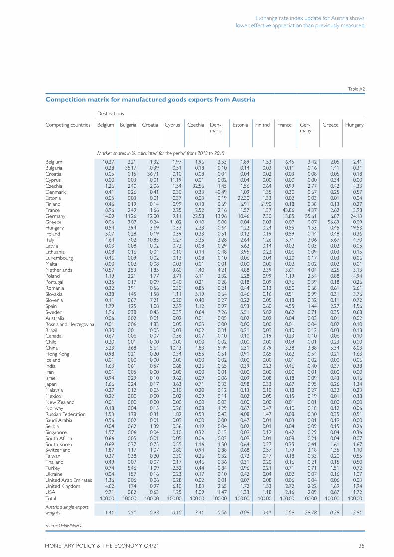
Exchange rate index update for Austria shows lower effective appreciation than previously measured
MONETARY POLICY & THE ECONOMY Q4/21 35
Table A1 continued
Exchange rate index update for Austria – new weighting scheme
Competing countries Austrian imports Exports and imports
Goods Services Total Manu-factured goods
Raw materials, energy products
Food Goods Services Total
Country weights in %, calculated for the period from 2013 to 2015
Belgium 1.52 1.77 1.58 2.14 0.41 1.37 1.91 1.69 1.85Bulgaria 0.31 1.07 0.49 0.35 0.16 0.36 0.33 0.75 0.44Croatia 0.43 2.33 0.88 0.46 0.50 0.80 0.49 1.48 0.75Cyprus 0.03 0.44 0.13 0.03 0.01 0.09 0.03 0.38 0.12Czechia 4.17 2.96 3.88 3.22 6.70 2.77 3.54 2.63 3.30Denmark 0.41 0.39 0.41 0.55 0.15 0.70 0.52 0.52 0.52Estonia 0.03 0.17 0.06 0.05 0.04 0.04 0.05 0.11 0.07Finland 0.34 1.12 0.53 0.48 0.16 0.18 0.42 0.83 0.53France 2.83 2.42 2.73 4.21 1.19 2.83 3.80 2.34 3.42Germany 37.70 31.14 36.14 31.07 28.01 36.23 31.14 36.29 32.50Greece 0.15 0.99 0.35 0.19 0.10 0.69 0.22 0.59 0.31Hungary 2.82 3.46 2.98 2.02 4.55 4.62 2.46 2.97 2.59Ireland 0.54 1.38 0.74 0.69 0.07 0.24 0.60 0.95 0.69Italy 6.24 5.67 6.10 6.50 7.29 12.27 7.00 5.24 6.54Latvia 0.02 0.14 0.05 0.05 0.04 0.07 0.05 0.11 0.07Lithuania 0.07 0.41 0.15 0.11 0.06 0.16 0.11 0.23 0.14Luxembourg 0.19 1.08 0.40 0.18 0.02 0.09 0.16 0.90 0.35Malta 0.01 0.23 0.06 0.02 0.01 0.05 0.02 0.22 0.07Netherlands 2.68 2.68 2.68 2.89 1.63 3.76 2.82 3.46 2.99Poland 2.09 2.55 2.20 2.61 1.71 2.92 2.54 1.97 2.39Portugal 0.38 0.45 0.39 0.43 0.09 0.14 0.37 0.29 0.35Romania 0.91 2.22 1.22 1.13 0.82 0.90 1.08 1.81 1.27Slovakia 2.28 3.02 2.45 1.66 4.67 1.86 1.98 2.23 2.05Slovenia 1.30 1.85 1.43 0.95 4.22 2.14 1.37 1.44 1.39Spain 1.70 1.89 1.75 2.13 0.41 2.38 1.98 1.28 1.80Sweden 0.97 1.96 1.21 1.20 0.53 0.58 1.09 1.69 1.25Australia 0.06 0.24 0.10 0.24 0.12 0.43 0.24 0.26 0.25Bosnia and Herzegovina 0.34 0.28 0.33 0.25 0.35 0.28 0.26 0.24 0.26Brazil 0.26 0.27 0.27 0.45 0.47 0.84 0.48 0.22 0.41Canada 0.31 0.50 0.35 0.58 0.21 0.11 0.51 0.44 0.49Chile 0.10 0.09 0.09 0.08 0.18 0.26 0.10 0.10 0.10China 5.68 0.87 4.54 7.68 0.91 0.55 6.48 0.92 5.02Hong Kong 0.06 0.26 0.11 0.46 0.06 0.09 0.39 0.22 0.35Iceland 0.01 0.04 0.02 0.02 0.00 0.01 0.01 0.03 0.02India 0.49 0.34 0.46 0.84 0.21 0.21 0.73 0.28 0.61Iran 0.01 0.05 0.02 0.09 0.02 0.08 0.08 0.07 0.08Israel 0.12 0.19 0.14 0.22 0.09 0.21 0.21 0.20 0.20Japan 1.36 0.27 1.10 1.92 0.44 0.42 1.66 0.38 1.33Malaysia 0.24 0.29 0.25 0.42 0.02 0.03 0.35 0.18 0.30Mexico 0.28 0.12 0.24 0.51 0.49 0.10 0.47 0.14 0.39New Zealand 0.04 0.07 0.04 0.06 0.01 0.12 0.06 0.07 0.06Norway 0.21 0.28 0.23 0.27 0.33 0.27 0.27 0.36 0.29Russian Federation 2.04 1.70 1.96 1.32 9.01 0.91 2.07 1.98 2.05Saudi Arabia 0.28 0.13 0.24 0.23 1.32 0.18 0.33 0.21 0.30Serbia 0.27 0.45 0.32 0.28 0.28 0.60 0.30 0.39 0.33Singapore 0.08 0.17 0.10 0.39 0.00 0.03 0.33 0.17 0.29South Africa 0.32 0.44 0.35 0.27 1.18 0.32 0.36 0.27 0.34South Korea 0.59 0.14 0.48 1.23 0.21 0.31 1.06 0.19 0.83Switzerland 4.15 4.54 4.24 4.18 2.68 3.99 4.01 6.12 4.57Taiwan 0.43 0.15 0.36 0.61 0.05 0.05 0.52 0.13 0.42Thailand 0.40 0.34 0.38 0.50 0.07 0.18 0.44 0.21 0.38Turkey 1.02 1.21 1.06 1.27 0.60 1.30 1.20 1.15 1.19Ukraine 0.45 0.74 0.52 0.26 1.60 0.37 0.41 0.57 0.45United Arab Emirates 0.12 0.61 0.24 0.29 0.03 0.20 0.25 0.62 0.35United Kingdom 1.75 4.34 2.37 2.65 1.16 1.51 2.42 4.04 2.84USA 8.40 7.08 8.09 7.14 14.35 7.78 7.92 7.44 7.79Total 100.00 100.00 100.00 100.00 100.00 100.00 100.00 100.00 100.00
Source: OeNB/WIFO.
Table A2
Competition matrix for manufactured goods exports from Austria
Destinations
Competing countries Belgium Bulgaria Croatia Cyprus Czechia Den-mark
Estonia Finland France Ger-many
Greece Hungary
Market shares in %: calculated for the period from 2013 to 2015
Belgium 10.27 2.21 1.32 1.97 1.96 2.53 1.89 1.53 6.45 3.42 2.05 2.41Bulgaria 0.28 35.17 0.39 0.51 0.18 0.10 0.14 0.03 0.11 0.16 1.41 0.31Croatia 0.05 0.15 36.71 0.10 0.08 0.04 0.04 0.02 0.03 0.08 0.05 0.18Cyprus 0.00 0.03 0.01 11.19 0.01 0.02 0.04 0.00 0.00 0.00 0.34 0.00Czechia 1.26 2.40 2.06 1.54 32.56 1.45 1.56 0.64 0.99 2.77 0.42 4.33Denmark 0.41 0.26 0.41 0.30 0.33 40.49 1.09 1.35 0.30 0.67 0.25 0.57Estonia 0.05 0.03 0.01 0.37 0.03 0.19 22.30 1.33 0.02 0.03 0.01 0.04Finland 0.46 0.19 0.14 0.99 0.18 0.69 6.91 61.90 0.18 0.38 0.13 0.27France 8.96 2.49 1.66 2.25 2.52 2.16 1.57 1.37 43.86 4.37 2.62 3.98Germany 14.09 11.26 12.00 9.11 22.58 13.96 10.46 7.30 13.85 55.61 6.87 24.13Greece 0.06 3.07 0.24 11.02 0.10 0.08 0.04 0.03 0.07 0.07 56.63 0.09Hungary 0.54 2.94 3.69 0.33 2.23 0.64 1.22 0.24 0.55 1.53 0.45 19.53Ireland 5.07 0.28 0.19 0.39 0.33 0.51 0.12 0.19 0.59 0.44 0.48 0.36Italy 4.64 7.02 10.83 6.27 3.25 2.28 2.64 1.26 5.71 3.06 5.67 4.70Latvia 0.03 0.08 0.02 0.72 0.08 0.29 5.62 0.14 0.02 0.03 0.02 0.05Lithuania 0.08 0.16 0.04 0.10 0.14 0.48 3.95 0.22 0.06 0.09 0.03 0.15Luxembourg 0.46 0.09 0.02 0.13 0.08 0.10 0.06 0.04 0.20 0.17 0.03 0.06Malta 0.00 0.02 0.08 0.03 0.01 0.01 0.00 0.00 0.02 0.02 0.02 0.01Netherlands 10.57 2.53 1.85 3.60 4.40 4.21 4.88 2.39 3.61 4.04 2.25 3.13Poland 1.19 2.21 1.77 3.71 6.11 2.32 6.28 0.99 1.19 2.54 0.88 4.94Portugal 0.35 0.17 0.09 0.40 0.21 0.28 0.18 0.09 0.76 0.39 0.18 0.26Romania 0.32 3.91 0.56 0.30 0.85 0.21 0.44 0.13 0.50 0.68 0.61 2.61Slovakia 0.38 1.45 1.58 1.11 5.19 0.64 0.46 0.16 0.51 0.99 0.31 3.76Slovenia 0.11 0.67 7.21 0.20 0.40 0.27 0.22 0.05 0.18 0.32 0.11 0.72Spain 1.79 1.25 1.08 2.59 1.12 0.97 0.93 0.60 4.55 1.44 2.27 1.56Sweden 1.96 0.38 0.45 0.39 0.64 7.26 5.51 5.82 0.62 0.71 0.35 0.68Australia 0.06 0.02 0.01 0.02 0.01 0.05 0.02 0.02 0.04 0.03 0.01 0.02Bosnia and Herzegovina 0.01 0.06 1.83 0.05 0.05 0.00 0.00 0.00 0.01 0.04 0.02 0.10Brazil 0.30 0.01 0.05 0.03 0.02 0.31 0.21 0.09 0.10 0.12 0.03 0.18Canada 0.67 0.06 0.07 0.36 0.07 0.10 0.10 0.19 0.23 0.10 0.06 0.10Chile 0.20 0.01 0.00 0.00 0.00 0.02 0.00 0.00 0.09 0.01 0.23 0.00China 5.23 3.68 5.64 10.43 4.83 5.49 6.31 3.79 3.38 3.88 5.34 6.03Hong Kong 0.98 0.21 0.20 0.34 0.55 0.51 0.91 0.65 0.62 0.54 0.21 1.63Iceland 0.01 0.00 0.00 0.00 0.00 0.02 0.00 0.00 0.01 0.02 0.00 0.06India 1.63 0.61 0.57 0.68 0.26 0.65 0.39 0.23 0.46 0.40 0.37 0.38Iran 0.01 0.05 0.00 0.00 0.00 0.01 0.00 0.00 0.00 0.01 0.00 0.00Israel 0.94 0.29 0.10 9.62 0.09 0.06 0.09 0.08 0.18 0.09 0.43 0.16Japan 1.66 0.24 0.17 3.63 0.71 0.33 0.98 0.33 0.67 0.95 0.26 1.34Malaysia 0.27 0.12 0.05 0.10 0.20 0.12 0.13 0.10 0.18 0.27 0.32 0.23Mexico 0.22 0.00 0.00 0.02 0.09 0.11 0.02 0.05 0.15 0.19 0.01 0.38New Zealand 0.01 0.00 0.00 0.00 0.00 0.03 0.00 0.00 0.01 0.01 0.00 0.00Norway 0.18 0.04 0.15 0.26 0.08 1.29 0.67 0.47 0.10 0.18 0.12 0.06Russian Federation 1.53 1.78 0.31 1.82 0.53 0.43 4.08 1.47 0.08 0.30 0.35 0.51Saudi Arabia 0.56 0.02 0.01 0.09 0.00 0.00 0.47 0.01 0.03 0.01 0.19 0.00Serbia 0.04 0.62 1.39 0.56 0.19 0.04 0.02 0.01 0.04 0.09 0.15 0.26Singapore 1.57 0.06 0.04 0.10 0.32 0.13 0.09 0.12 0.42 0.29 0.04 0.36South Africa 0.66 0.05 0.01 0.05 0.06 0.02 0.09 0.01 0.08 0.21 0.04 0.07South Korea 0.69 0.37 0.75 0.55 1.16 1.50 0.64 0.27 0.35 0.41 1.61 1.67Switzerland 1.87 1.17 1.07 0.80 0.94 0.88 0.68 0.57 1.79 2.18 1.35 1.10Taiwan 0.37 0.38 0.20 0.30 0.26 0.32 0.72 0.47 0.18 0.33 0.20 0.55Thailand 0.49 0.07 0.07 0.17 0.46 0.36 0.31 0.20 0.16 0.21 0.15 0.50Turkey 0.74 5.46 1.09 2.52 0.44 0.84 0.96 0.21 0.71 0.71 1.51 0.72Ukraine 0.04 1.57 0.16 0.23 0.17 0.10 0.42 0.04 0.02 0.07 0.16 1.07United Arab Emirates 1.36 0.06 0.06 0.28 0.02 0.01 0.07 0.08 0.06 0.04 0.06 0.03United Kingdom 4.62 1.74 0.97 6.10 1.83 2.65 1.72 1.53 2.72 2.22 1.69 1.94USA 9.71 0.82 0.63 1.25 1.09 1.47 1.33 1.18 2.16 2.09 0.67 1.72Total 100.00 100.00 100.00 100.00 100.00 100.00 100.00 100.00 100.00 100.00 100.00 100.00
Austria’s single export weights 1.41 0.51 0.93 0.10 3.41 0.56 0.09 0.41 5.09 29.78 0.29 2.91
Source: OeNB/WIFO.

Exchange rate index update for Austria shows lower effective appreciation than previously measured
36 OESTERREICHISCHE NATIONALBANK
Table A2 continued
Competition matrix for manufactured goods exports from Austria
Destinations
Competing countries Ireland Italy Latvia Lithuania Luxem-bourg
Malta Nether-lands
Poland Portugal Romania Slovakia Slovenia
Market shares in %: calculated for the period from 2013 to 2015
Belgium 1.88 2.08 2.01 3.11 17.07 0.94 6.13 2.30 2.10 1.38 1.39 1.95Bulgaria 0.02 0.22 0.17 0.17 0.01 0.29 0.08 0.15 0.04 1.46 0.20 0.30Croatia 0.01 0.11 0.06 0.05 0.29 0.07 0.04 0.05 0.04 0.10 0.20 2.61Cyprus 0.07 0.00 0.04 0.13 0.00 0.64 0.04 0.00 0.00 0.01 0.04 0.01Czechia 0.55 0.57 1.57 1.93 0.62 0.36 0.88 2.82 0.56 1.82 12.75 1.94Denmark 0.61 0.14 1.47 1.30 0.17 0.37 0.50 0.57 0.16 0.25 0.29 0.23Estonia 0.02 0.01 4.51 1.90 0.02 0.02 0.03 0.07 0.01 0.02 0.03 0.02Finland 0.25 0.13 1.74 1.04 0.10 0.22 0.65 0.48 0.13 0.16 0.14 0.24France 2.11 3.08 1.50 1.70 6.57 4.26 2.88 2.71 4.47 3.81 3.37 2.82Germany 6.24 6.26 9.67 10.02 19.70 5.50 13.02 16.34 8.69 11.34 15.66 14.08Greece 0.04 0.14 0.07 0.07 0.02 0.59 0.06 0.09 0.11 0.58 0.04 0.09Hungary 0.19 0.41 0.87 0.71 0.39 0.10 0.53 1.20 0.32 3.48 5.10 2.28Ireland 46.63 0.27 0.10 0.14 0.36 0.19 0.90 0.36 0.43 0.42 0.09 0.15Italy 1.23 69.11 2.90 3.30 2.25 10.98 1.94 4.05 4.14 6.92 3.42 9.98Latvia 0.01 0.01 27.27 5.04 0.05 0.04 0.02 0.14 0.01 0.02 0.07 0.03Lithuania 0.08 0.03 7.56 35.61 0.02 0.04 0.08 0.32 0.09 0.07 0.09 0.06Luxembourg 0.05 0.05 0.08 0.05 26.34 0.10 0.13 0.10 0.04 0.05 0.07 0.11Malta 0.01 0.01 0.00 0.01 0.00 11.08 0.01 0.01 0.01 0.03 0.01 0.00Netherlands 2.95 1.77 2.34 2.42 4.07 1.82 30.93 3.27 2.72 1.75 1.83 2.21Poland 0.44 0.83 8.57 8.40 0.91 0.55 1.24 46.03 0.71 2.33 4.78 1.74Portugal 0.22 0.16 0.14 0.16 0.21 0.22 0.32 0.16 47.00 0.33 0.18 0.11Romania 0.11 0.70 0.16 0.19 0.08 0.12 0.27 0.52 0.16 48.58 1.24 0.84Slovakia 0.13 0.39 1.16 0.63 0.35 0.17 0.39 2.01 0.24 1.53 33.29 1.77Slovenia 0.04 0.25 0.26 0.29 0.10 0.05 0.09 0.30 0.08 0.38 0.54 32.29Spain 1.19 1.59 0.77 0.90 1.23 1.30 1.07 1.42 17.25 1.68 0.93 1.29Sweden 0.44 0.35 2.21 2.38 0.47 0.25 1.11 1.08 0.41 0.28 0.31 0.36Australia 0.04 0.02 0.03 0.01 0.02 0.01 0.09 0.01 0.01 0.03 0.00 0.03Bosnia and Herzegovina 0.00 0.07 0.00 0.00 0.15 0.01 0.02 0.01 0.00 0.06 0.08 1.10Brazil 0.33 0.14 0.03 0.06 0.08 0.03 0.96 0.04 0.29 0.04 0.03 0.05Canada 0.36 0.12 0.35 0.20 0.47 5.21 0.35 0.09 0.15 0.05 0.03 0.07Chile 0.00 0.12 0.00 0.00 0.00 0.00 0.19 0.00 0.00 0.00 0.00 0.00China 2.80 2.96 7.62 5.62 9.01 24.48 12.20 4.64 3.01 2.87 3.60 6.40Hong Kong 0.28 0.34 0.65 0.34 0.57 0.20 1.23 0.35 0.29 0.29 0.31 0.21Iceland 0.00 0.01 0.00 0.00 0.00 0.00 0.26 0.00 0.01 0.00 0.01 0.00India 0.56 0.45 0.52 0.24 0.04 1.09 0.67 0.32 0.64 0.30 0.16 0.68Iran 0.00 0.04 0.00 0.00 0.00 0.00 0.01 0.00 0.03 0.00 0.00 0.00Israel 0.12 0.10 0.28 0.15 0.09 2.01 0.39 0.07 0.12 0.11 0.03 0.38Japan 1.26 0.36 0.30 0.22 1.16 1.91 2.44 0.54 0.39 0.29 0.34 0.29Malaysia 0.15 0.07 0.28 0.14 0.03 0.45 1.00 0.13 0.06 0.07 0.12 0.35Mexico 0.22 0.08 0.01 0.10 0.07 0.00 0.21 0.06 0.04 0.06 0.02 0.01New Zealand 0.02 0.02 0.01 0.01 0.00 0.01 0.04 0.00 0.00 0.00 0.00 0.01Norway 0.33 0.05 0.26 0.36 0.13 0.58 0.59 0.30 0.10 0.14 0.03 0.03Russian Federation 0.18 0.34 4.71 3.57 0.02 0.37 1.71 0.51 0.14 0.25 0.48 0.24Saudi Arabia 0.01 0.09 0.01 0.01 0.00 0.89 0.09 0.12 0.04 0.01 0.00 0.02Serbia 0.01 0.25 0.03 0.08 0.03 0.03 0.02 0.09 0.03 0.34 0.25 1.17Singapore 0.50 0.05 0.07 0.07 0.08 0.83 1.24 0.07 0.05 0.06 0.04 0.09South Africa 0.06 0.06 0.01 0.06 0.09 0.13 0.17 0.04 0.04 0.03 0.00 0.06South Korea 0.42 0.37 0.62 0.77 1.44 12.74 0.54 1.17 0.47 0.50 5.08 5.18Switzerland 1.09 1.41 0.86 0.63 0.90 0.41 0.98 0.74 0.98 0.75 0.68 1.45Taiwan 0.21 0.19 0.81 0.45 0.07 0.30 0.86 0.26 0.21 0.13 0.41 0.45Thailand 0.43 0.11 0.16 0.10 0.02 0.14 0.77 0.14 0.14 0.10 0.19 0.13Turkey 0.43 0.64 0.97 1.22 0.19 1.82 0.50 0.70 0.60 2.51 0.57 2.36Ukraine 0.00 0.17 0.71 0.57 0.02 0.02 0.07 0.47 0.07 0.32 0.33 0.04United Arab Emirates 0.01 0.06 0.08 0.05 0.15 0.19 0.22 0.03 0.03 0.02 0.00 0.01United Kingdom 17.88 1.30 1.66 1.51 1.32 5.12 3.33 1.73 1.57 1.33 0.84 1.03USA 6.78 1.32 1.75 1.80 2.40 0.72 5.56 0.80 0.53 0.56 0.31 0.59Total 100.00 100.00 100.00 100.00 100.00 100.00 100.00 100.00 100.00 100.00 100.00 100.00
Austria’s single export weights 0.42 5.16 0.12 0.14 0.15 0.03 1.61 3.20 0.25 1.54 1.93 1.43
Source: OeNB/WIFO.
Table A2 continued
Competition matrix for manufactured goods exports from Austria
Destinations
Competing countries Spain Sweden Australia Bosnia and Herze-govina
Brazil Canada Chile China Hong Kong
Iceland India Iran
Market shares in %: calculated for the period from 2013 to 2015
Belgium 1.81 2.57 0.62 0.77 0.39 0.33 0.68 0.07 0.43 1.82 0.88 0.21Bulgaria 0.06 0.06 0.01 0.57 0.00 0.01 0.01 0.01 0.01 0.03 0.00 0.05Croatia 0.03 0.03 0.00 7.91 0.00 0.00 0.00 0.00 0.00 0.03 0.00 0.01Cyprus 0.00 0.00 0.00 0.02 0.00 0.00 0.00 0.00 0.00 0.00 0.00 0.00Czechia 0.73 1.06 0.18 1.56 0.04 0.04 0.10 0.02 0.05 1.12 0.05 0.02Denmark 0.23 3.19 0.17 0.17 0.08 0.08 0.28 0.02 0.04 8.13 0.02 0.05Estonia 0.02 1.01 0.00 0.02 0.00 0.00 0.00 0.00 0.00 0.33 0.00 0.00Finland 0.16 2.04 0.16 0.05 0.06 0.07 0.35 0.02 0.03 0.86 0.04 0.03France 5.38 2.29 0.83 1.24 0.58 0.44 1.12 0.17 0.74 1.70 0.28 0.41Germany 7.37 10.44 2.92 11.45 1.39 1.64 4.00 0.84 0.96 9.43 0.93 1.43Greece 0.08 0.05 0.03 0.32 0.00 0.01 0.02 0.00 0.01 0.05 0.00 0.01Hungary 0.54 0.46 0.10 3.14 0.04 0.04 0.08 0.02 0.04 0.28 0.02 0.02Ireland 0.71 0.39 0.26 0.19 0.03 0.13 0.13 0.01 0.08 0.65 0.05 0.05Italy 3.76 1.83 1.19 8.79 0.60 0.49 1.49 0.12 0.96 2.93 0.31 1.00Latvia 0.01 0.18 0.00 0.04 0.00 0.00 0.00 0.00 0.00 0.34 0.00 0.00Lithuania 0.04 0.38 0.01 0.03 0.00 0.01 0.00 0.00 0.01 0.54 0.00 0.00Luxembourg 0.05 0.09 0.01 0.01 0.01 0.02 0.01 0.00 0.01 0.06 0.00 0.00Malta 0.01 0.01 0.00 0.00 0.00 0.01 0.00 0.00 0.04 0.09 0.00 0.00Netherlands 2.09 2.98 0.64 1.27 0.28 0.23 0.57 0.06 0.17 8.75 0.16 0.26Poland 0.85 2.08 0.16 1.84 0.05 0.13 0.11 0.02 0.05 1.35 0.03 0.03Portugal 1.89 0.19 0.03 0.03 0.04 0.04 0.15 0.01 0.02 0.38 0.01 0.01Romania 0.25 0.25 0.01 0.99 0.03 0.02 0.03 0.00 0.01 0.06 0.02 0.08Slovakia 0.35 0.51 0.09 1.17 0.01 0.03 0.05 0.02 0.01 0.30 0.00 0.01Slovenia 0.07 0.13 0.03 7.78 0.01 0.01 0.03 0.00 0.01 0.06 0.01 0.02Spain 61.06 0.87 0.54 0.63 0.33 0.17 2.01 0.03 0.12 0.68 0.10 0.22Sweden 0.37 54.55 0.44 0.30 0.13 0.15 0.48 0.05 0.08 6.03 0.10 0.19Australia 0.02 0.03 55.91 0.00 0.02 0.05 0.17 0.04 0.17 0.05 0.04 0.00Bosnia and Herzegovina 0.01 0.02 0.00 32.96 0.00 0.00 0.00 0.00 0.00 0.00 0.00 0.00Brazil 0.10 0.08 0.09 0.01 85.04 0.09 3.31 0.03 0.06 0.01 0.05 0.01Canada 0.07 0.12 0.34 0.02 0.18 51.01 0.66 0.05 0.15 0.54 0.11 0.01Chile 0.05 0.01 0.16 0.00 0.22 0.09 41.73 0.09 0.00 0.28 0.01 0.00China 3.83 3.03 11.09 1.88 3.49 4.32 18.33 90.61 51.40 3.54 4.55 13.11Hong Kong 0.36 0.41 1.32 0.26 0.19 0.42 0.77 2.46 12.68 0.20 1.04 0.08Iceland 0.04 0.00 0.00 0.00 0.00 0.00 0.01 0.00 0.00 30.03 0.00 0.00India 0.53 0.31 0.59 0.20 0.29 0.27 0.90 0.08 1.92 0.52 83.96 1.32Iran 0.02 0.00 0.00 0.01 0.00 0.00 0.00 0.04 0.00 0.00 0.17 67.08Israel 0.18 0.06 0.16 0.02 0.10 0.08 0.20 0.03 0.84 0.15 0.19 0.00Japan 0.42 0.52 3.44 0.07 0.50 1.18 2.01 1.10 3.95 1.06 0.66 0.16Malaysia 0.07 0.13 1.29 0.00 0.09 0.11 0.23 0.20 1.46 0.03 0.34 0.13Mexico 0.11 0.04 0.18 0.00 0.46 1.30 2.41 0.03 0.08 0.00 0.03 0.00New Zealand 0.00 0.00 0.87 0.00 0.01 0.02 0.06 0.00 0.02 0.02 0.01 0.00Norway 0.11 1.20 0.07 0.02 0.04 0.04 0.08 0.02 0.02 6.19 0.01 0.00Russian Federation 0.14 0.19 0.02 0.28 0.20 0.05 0.03 0.04 0.11 0.50 0.33 0.37Saudi Arabia 0.14 0.04 0.11 0.00 0.03 0.00 0.08 0.07 0.04 0.04 0.25 0.07Serbia 0.02 0.02 0.00 8.67 0.00 0.00 0.00 0.00 0.00 0.01 0.00 0.01Singapore 0.06 0.04 1.90 0.02 0.19 0.14 0.09 0.42 5.37 0.03 0.83 0.09South Africa 0.09 0.06 0.21 0.01 0.05 0.03 0.08 0.02 0.15 0.06 0.05 0.01South Korea 0.37 0.36 1.80 0.20 0.87 0.73 2.80 1.33 3.89 0.68 0.96 2.89Switzerland 1.06 0.62 0.68 0.74 0.23 0.50 0.37 0.09 1.20 0.46 0.18 0.28Taiwan 0.17 0.26 0.81 0.02 0.16 0.35 0.43 0.76 5.49 0.17 0.27 0.47Thailand 0.12 0.19 2.59 0.02 0.19 0.12 0.81 0.16 1.64 0.04 0.41 0.15Turkey 0.76 0.47 0.11 3.47 0.07 0.08 0.27 0.01 0.05 0.75 0.03 2.13Ukraine 0.03 0.03 0.01 0.07 0.01 0.01 0.00 0.00 0.00 0.01 0.03 0.10United Arab Emirates 0.05 0.01 0.07 0.03 0.01 0.02 0.07 0.02 0.48 0.03 0.64 7.27United Kingdom 1.94 2.72 1.60 0.44 0.37 0.76 0.91 0.16 1.11 6.46 0.49 0.08USA 1.21 1.40 6.17 0.27 2.87 34.12 11.47 0.65 3.84 2.15 1.30 0.06Total 100.00 100.00 100.00 100.00 100.00 100.00 100.00 100.00 100.00 100.00 100.00 100.00
Austria’s single export weights 1.76 1.17 0.62 0.26 0.62 0.87 0.14 2.75 0.46 0.02 0.55 0.19
Source: OeNB/WIFO.

Exchange rate index update for Austria shows lower effective appreciation than previously measured
MONETARY POLICY & THE ECONOMY Q4/21 37
Table A2 continued
Competition matrix for manufactured goods exports from Austria
Destinations
Competing countries Ireland Italy Latvia Lithuania Luxem-bourg
Malta Nether-lands
Poland Portugal Romania Slovakia Slovenia
Market shares in %: calculated for the period from 2013 to 2015
Belgium 1.88 2.08 2.01 3.11 17.07 0.94 6.13 2.30 2.10 1.38 1.39 1.95Bulgaria 0.02 0.22 0.17 0.17 0.01 0.29 0.08 0.15 0.04 1.46 0.20 0.30Croatia 0.01 0.11 0.06 0.05 0.29 0.07 0.04 0.05 0.04 0.10 0.20 2.61Cyprus 0.07 0.00 0.04 0.13 0.00 0.64 0.04 0.00 0.00 0.01 0.04 0.01Czechia 0.55 0.57 1.57 1.93 0.62 0.36 0.88 2.82 0.56 1.82 12.75 1.94Denmark 0.61 0.14 1.47 1.30 0.17 0.37 0.50 0.57 0.16 0.25 0.29 0.23Estonia 0.02 0.01 4.51 1.90 0.02 0.02 0.03 0.07 0.01 0.02 0.03 0.02Finland 0.25 0.13 1.74 1.04 0.10 0.22 0.65 0.48 0.13 0.16 0.14 0.24France 2.11 3.08 1.50 1.70 6.57 4.26 2.88 2.71 4.47 3.81 3.37 2.82Germany 6.24 6.26 9.67 10.02 19.70 5.50 13.02 16.34 8.69 11.34 15.66 14.08Greece 0.04 0.14 0.07 0.07 0.02 0.59 0.06 0.09 0.11 0.58 0.04 0.09Hungary 0.19 0.41 0.87 0.71 0.39 0.10 0.53 1.20 0.32 3.48 5.10 2.28Ireland 46.63 0.27 0.10 0.14 0.36 0.19 0.90 0.36 0.43 0.42 0.09 0.15Italy 1.23 69.11 2.90 3.30 2.25 10.98 1.94 4.05 4.14 6.92 3.42 9.98Latvia 0.01 0.01 27.27 5.04 0.05 0.04 0.02 0.14 0.01 0.02 0.07 0.03Lithuania 0.08 0.03 7.56 35.61 0.02 0.04 0.08 0.32 0.09 0.07 0.09 0.06Luxembourg 0.05 0.05 0.08 0.05 26.34 0.10 0.13 0.10 0.04 0.05 0.07 0.11Malta 0.01 0.01 0.00 0.01 0.00 11.08 0.01 0.01 0.01 0.03 0.01 0.00Netherlands 2.95 1.77 2.34 2.42 4.07 1.82 30.93 3.27 2.72 1.75 1.83 2.21Poland 0.44 0.83 8.57 8.40 0.91 0.55 1.24 46.03 0.71 2.33 4.78 1.74Portugal 0.22 0.16 0.14 0.16 0.21 0.22 0.32 0.16 47.00 0.33 0.18 0.11Romania 0.11 0.70 0.16 0.19 0.08 0.12 0.27 0.52 0.16 48.58 1.24 0.84Slovakia 0.13 0.39 1.16 0.63 0.35 0.17 0.39 2.01 0.24 1.53 33.29 1.77Slovenia 0.04 0.25 0.26 0.29 0.10 0.05 0.09 0.30 0.08 0.38 0.54 32.29Spain 1.19 1.59 0.77 0.90 1.23 1.30 1.07 1.42 17.25 1.68 0.93 1.29Sweden 0.44 0.35 2.21 2.38 0.47 0.25 1.11 1.08 0.41 0.28 0.31 0.36Australia 0.04 0.02 0.03 0.01 0.02 0.01 0.09 0.01 0.01 0.03 0.00 0.03Bosnia and Herzegovina 0.00 0.07 0.00 0.00 0.15 0.01 0.02 0.01 0.00 0.06 0.08 1.10Brazil 0.33 0.14 0.03 0.06 0.08 0.03 0.96 0.04 0.29 0.04 0.03 0.05Canada 0.36 0.12 0.35 0.20 0.47 5.21 0.35 0.09 0.15 0.05 0.03 0.07Chile 0.00 0.12 0.00 0.00 0.00 0.00 0.19 0.00 0.00 0.00 0.00 0.00China 2.80 2.96 7.62 5.62 9.01 24.48 12.20 4.64 3.01 2.87 3.60 6.40Hong Kong 0.28 0.34 0.65 0.34 0.57 0.20 1.23 0.35 0.29 0.29 0.31 0.21Iceland 0.00 0.01 0.00 0.00 0.00 0.00 0.26 0.00 0.01 0.00 0.01 0.00India 0.56 0.45 0.52 0.24 0.04 1.09 0.67 0.32 0.64 0.30 0.16 0.68Iran 0.00 0.04 0.00 0.00 0.00 0.00 0.01 0.00 0.03 0.00 0.00 0.00Israel 0.12 0.10 0.28 0.15 0.09 2.01 0.39 0.07 0.12 0.11 0.03 0.38Japan 1.26 0.36 0.30 0.22 1.16 1.91 2.44 0.54 0.39 0.29 0.34 0.29Malaysia 0.15 0.07 0.28 0.14 0.03 0.45 1.00 0.13 0.06 0.07 0.12 0.35Mexico 0.22 0.08 0.01 0.10 0.07 0.00 0.21 0.06 0.04 0.06 0.02 0.01New Zealand 0.02 0.02 0.01 0.01 0.00 0.01 0.04 0.00 0.00 0.00 0.00 0.01Norway 0.33 0.05 0.26 0.36 0.13 0.58 0.59 0.30 0.10 0.14 0.03 0.03Russian Federation 0.18 0.34 4.71 3.57 0.02 0.37 1.71 0.51 0.14 0.25 0.48 0.24Saudi Arabia 0.01 0.09 0.01 0.01 0.00 0.89 0.09 0.12 0.04 0.01 0.00 0.02Serbia 0.01 0.25 0.03 0.08 0.03 0.03 0.02 0.09 0.03 0.34 0.25 1.17Singapore 0.50 0.05 0.07 0.07 0.08 0.83 1.24 0.07 0.05 0.06 0.04 0.09South Africa 0.06 0.06 0.01 0.06 0.09 0.13 0.17 0.04 0.04 0.03 0.00 0.06South Korea 0.42 0.37 0.62 0.77 1.44 12.74 0.54 1.17 0.47 0.50 5.08 5.18Switzerland 1.09 1.41 0.86 0.63 0.90 0.41 0.98 0.74 0.98 0.75 0.68 1.45Taiwan 0.21 0.19 0.81 0.45 0.07 0.30 0.86 0.26 0.21 0.13 0.41 0.45Thailand 0.43 0.11 0.16 0.10 0.02 0.14 0.77 0.14 0.14 0.10 0.19 0.13Turkey 0.43 0.64 0.97 1.22 0.19 1.82 0.50 0.70 0.60 2.51 0.57 2.36Ukraine 0.00 0.17 0.71 0.57 0.02 0.02 0.07 0.47 0.07 0.32 0.33 0.04United Arab Emirates 0.01 0.06 0.08 0.05 0.15 0.19 0.22 0.03 0.03 0.02 0.00 0.01United Kingdom 17.88 1.30 1.66 1.51 1.32 5.12 3.33 1.73 1.57 1.33 0.84 1.03USA 6.78 1.32 1.75 1.80 2.40 0.72 5.56 0.80 0.53 0.56 0.31 0.59Total 100.00 100.00 100.00 100.00 100.00 100.00 100.00 100.00 100.00 100.00 100.00 100.00
Austria’s single export weights 0.42 5.16 0.12 0.14 0.15 0.03 1.61 3.20 0.25 1.54 1.93 1.43
Source: OeNB/WIFO.
Table A2 continued
Competition matrix for manufactured goods exports from Austria
Destinations
Competing countries Spain Sweden Australia Bosnia and Herze-govina
Brazil Canada Chile China Hong Kong
Iceland India Iran
Market shares in %: calculated for the period from 2013 to 2015
Belgium 1.81 2.57 0.62 0.77 0.39 0.33 0.68 0.07 0.43 1.82 0.88 0.21Bulgaria 0.06 0.06 0.01 0.57 0.00 0.01 0.01 0.01 0.01 0.03 0.00 0.05Croatia 0.03 0.03 0.00 7.91 0.00 0.00 0.00 0.00 0.00 0.03 0.00 0.01Cyprus 0.00 0.00 0.00 0.02 0.00 0.00 0.00 0.00 0.00 0.00 0.00 0.00Czechia 0.73 1.06 0.18 1.56 0.04 0.04 0.10 0.02 0.05 1.12 0.05 0.02Denmark 0.23 3.19 0.17 0.17 0.08 0.08 0.28 0.02 0.04 8.13 0.02 0.05Estonia 0.02 1.01 0.00 0.02 0.00 0.00 0.00 0.00 0.00 0.33 0.00 0.00Finland 0.16 2.04 0.16 0.05 0.06 0.07 0.35 0.02 0.03 0.86 0.04 0.03France 5.38 2.29 0.83 1.24 0.58 0.44 1.12 0.17 0.74 1.70 0.28 0.41Germany 7.37 10.44 2.92 11.45 1.39 1.64 4.00 0.84 0.96 9.43 0.93 1.43Greece 0.08 0.05 0.03 0.32 0.00 0.01 0.02 0.00 0.01 0.05 0.00 0.01Hungary 0.54 0.46 0.10 3.14 0.04 0.04 0.08 0.02 0.04 0.28 0.02 0.02Ireland 0.71 0.39 0.26 0.19 0.03 0.13 0.13 0.01 0.08 0.65 0.05 0.05Italy 3.76 1.83 1.19 8.79 0.60 0.49 1.49 0.12 0.96 2.93 0.31 1.00Latvia 0.01 0.18 0.00 0.04 0.00 0.00 0.00 0.00 0.00 0.34 0.00 0.00Lithuania 0.04 0.38 0.01 0.03 0.00 0.01 0.00 0.00 0.01 0.54 0.00 0.00Luxembourg 0.05 0.09 0.01 0.01 0.01 0.02 0.01 0.00 0.01 0.06 0.00 0.00Malta 0.01 0.01 0.00 0.00 0.00 0.01 0.00 0.00 0.04 0.09 0.00 0.00Netherlands 2.09 2.98 0.64 1.27 0.28 0.23 0.57 0.06 0.17 8.75 0.16 0.26Poland 0.85 2.08 0.16 1.84 0.05 0.13 0.11 0.02 0.05 1.35 0.03 0.03Portugal 1.89 0.19 0.03 0.03 0.04 0.04 0.15 0.01 0.02 0.38 0.01 0.01Romania 0.25 0.25 0.01 0.99 0.03 0.02 0.03 0.00 0.01 0.06 0.02 0.08Slovakia 0.35 0.51 0.09 1.17 0.01 0.03 0.05 0.02 0.01 0.30 0.00 0.01Slovenia 0.07 0.13 0.03 7.78 0.01 0.01 0.03 0.00 0.01 0.06 0.01 0.02Spain 61.06 0.87 0.54 0.63 0.33 0.17 2.01 0.03 0.12 0.68 0.10 0.22Sweden 0.37 54.55 0.44 0.30 0.13 0.15 0.48 0.05 0.08 6.03 0.10 0.19Australia 0.02 0.03 55.91 0.00 0.02 0.05 0.17 0.04 0.17 0.05 0.04 0.00Bosnia and Herzegovina 0.01 0.02 0.00 32.96 0.00 0.00 0.00 0.00 0.00 0.00 0.00 0.00Brazil 0.10 0.08 0.09 0.01 85.04 0.09 3.31 0.03 0.06 0.01 0.05 0.01Canada 0.07 0.12 0.34 0.02 0.18 51.01 0.66 0.05 0.15 0.54 0.11 0.01Chile 0.05 0.01 0.16 0.00 0.22 0.09 41.73 0.09 0.00 0.28 0.01 0.00China 3.83 3.03 11.09 1.88 3.49 4.32 18.33 90.61 51.40 3.54 4.55 13.11Hong Kong 0.36 0.41 1.32 0.26 0.19 0.42 0.77 2.46 12.68 0.20 1.04 0.08Iceland 0.04 0.00 0.00 0.00 0.00 0.00 0.01 0.00 0.00 30.03 0.00 0.00India 0.53 0.31 0.59 0.20 0.29 0.27 0.90 0.08 1.92 0.52 83.96 1.32Iran 0.02 0.00 0.00 0.01 0.00 0.00 0.00 0.04 0.00 0.00 0.17 67.08Israel 0.18 0.06 0.16 0.02 0.10 0.08 0.20 0.03 0.84 0.15 0.19 0.00Japan 0.42 0.52 3.44 0.07 0.50 1.18 2.01 1.10 3.95 1.06 0.66 0.16Malaysia 0.07 0.13 1.29 0.00 0.09 0.11 0.23 0.20 1.46 0.03 0.34 0.13Mexico 0.11 0.04 0.18 0.00 0.46 1.30 2.41 0.03 0.08 0.00 0.03 0.00New Zealand 0.00 0.00 0.87 0.00 0.01 0.02 0.06 0.00 0.02 0.02 0.01 0.00Norway 0.11 1.20 0.07 0.02 0.04 0.04 0.08 0.02 0.02 6.19 0.01 0.00Russian Federation 0.14 0.19 0.02 0.28 0.20 0.05 0.03 0.04 0.11 0.50 0.33 0.37Saudi Arabia 0.14 0.04 0.11 0.00 0.03 0.00 0.08 0.07 0.04 0.04 0.25 0.07Serbia 0.02 0.02 0.00 8.67 0.00 0.00 0.00 0.00 0.00 0.01 0.00 0.01Singapore 0.06 0.04 1.90 0.02 0.19 0.14 0.09 0.42 5.37 0.03 0.83 0.09South Africa 0.09 0.06 0.21 0.01 0.05 0.03 0.08 0.02 0.15 0.06 0.05 0.01South Korea 0.37 0.36 1.80 0.20 0.87 0.73 2.80 1.33 3.89 0.68 0.96 2.89Switzerland 1.06 0.62 0.68 0.74 0.23 0.50 0.37 0.09 1.20 0.46 0.18 0.28Taiwan 0.17 0.26 0.81 0.02 0.16 0.35 0.43 0.76 5.49 0.17 0.27 0.47Thailand 0.12 0.19 2.59 0.02 0.19 0.12 0.81 0.16 1.64 0.04 0.41 0.15Turkey 0.76 0.47 0.11 3.47 0.07 0.08 0.27 0.01 0.05 0.75 0.03 2.13Ukraine 0.03 0.03 0.01 0.07 0.01 0.01 0.00 0.00 0.00 0.01 0.03 0.10United Arab Emirates 0.05 0.01 0.07 0.03 0.01 0.02 0.07 0.02 0.48 0.03 0.64 7.27United Kingdom 1.94 2.72 1.60 0.44 0.37 0.76 0.91 0.16 1.11 6.46 0.49 0.08USA 1.21 1.40 6.17 0.27 2.87 34.12 11.47 0.65 3.84 2.15 1.30 0.06Total 100.00 100.00 100.00 100.00 100.00 100.00 100.00 100.00 100.00 100.00 100.00 100.00
Austria’s single export weights 1.76 1.17 0.62 0.26 0.62 0.87 0.14 2.75 0.46 0.02 0.55 0.19
Source: OeNB/WIFO.

Exchange rate index update for Austria shows lower effective appreciation than previously measured
38 OESTERREICHISCHE NATIONALBANK
Table A2 continued
Competition matrix for manufactured goods exports from Austria
Destinations
Competing countries Israel Japan Malaysia Mexico New Zealand
Norway Russian Federa-tion
Saudi Arabia
Serbia Singa-pore
South Africa
South Korea
Market shares in %: calculated for the period from 2013 to 2015
Belgium 2.95 0.16 0.20 0.21 0.43 1.39 0.61 0.83 1.01 0.41 1.07 0.11Bulgaria 0.06 0.00 0.01 0.00 0.01 0.03 0.07 0.02 1.44 0.01 0.02 0.00Croatia 0.04 0.00 0.00 0.00 0.00 0.05 0.04 0.02 1.88 0.00 0.01 0.00Cyprus 0.08 0.00 0.00 0.00 0.00 0.02 0.00 0.01 0.01 0.04 0.00 0.00Czechia 0.74 0.03 0.06 0.10 0.13 0.56 0.63 0.21 1.73 0.08 0.33 0.04Denmark 0.13 0.03 0.04 0.06 0.20 3.91 0.12 0.15 0.44 0.15 0.21 0.05Estonia 0.01 0.00 0.00 0.02 0.00 0.38 0.25 0.01 0.02 0.00 0.01 0.00Finland 0.11 0.03 0.06 0.05 0.11 1.26 0.61 0.16 0.15 0.09 0.23 0.07France 1.48 0.29 0.85 0.53 1.11 1.14 0.95 1.41 1.48 1.78 1.41 0.41Germany 4.70 0.88 1.91 1.93 2.32 7.01 4.53 4.47 9.32 2.48 7.23 1.44Greece 0.16 0.00 0.00 0.01 0.02 0.02 0.03 0.04 0.81 0.02 0.03 0.00Hungary 0.37 0.03 0.04 0.10 0.08 0.18 0.31 0.07 3.84 0.08 0.23 0.03Ireland 0.77 0.13 0.08 0.22 0.17 0.20 0.06 0.37 0.28 0.23 0.19 0.04Italy 2.83 0.26 0.42 0.65 0.86 1.28 1.44 2.08 7.96 0.73 1.42 0.36Latvia 0.01 0.00 0.00 0.00 0.01 0.20 0.10 0.00 0.02 0.00 0.01 0.00Lithuania 0.02 0.00 0.00 0.00 0.01 0.48 0.56 0.01 0.06 0.00 0.01 0.00Luxembourg 0.02 0.00 0.00 0.01 0.01 0.05 0.02 0.02 0.03 0.01 0.04 0.00Malta 0.00 0.00 0.00 0.00 0.00 0.00 0.00 0.01 0.03 0.09 0.00 0.00Netherlands 1.60 0.13 0.30 0.18 0.52 2.51 0.76 1.00 1.54 0.74 1.18 0.33Poland 0.40 0.02 0.06 0.09 0.12 2.50 0.99 0.15 3.17 0.27 0.38 0.04Portugal 0.12 0.00 0.01 0.04 0.03 0.10 0.03 0.06 0.04 0.02 0.10 0.01Romania 0.16 0.00 0.01 0.03 0.01 0.54 0.21 0.07 2.11 0.02 0.11 0.03Slovakia 0.24 0.01 0.01 0.03 0.06 0.18 0.34 0.07 1.58 0.01 0.07 0.01Slovenia 0.05 0.00 0.00 0.01 0.01 0.06 0.15 0.03 3.74 0.01 0.03 0.00Spain 1.57 0.08 0.19 0.68 0.51 0.66 0.32 1.23 0.65 0.22 0.94 0.08Sweden 0.35 0.07 0.12 0.11 0.26 10.10 0.35 0.54 0.57 0.27 0.61 0.09Australia 0.09 0.08 0.62 0.03 8.90 0.07 0.01 0.39 0.00 0.47 0.25 0.15Bosnia and Herzegovina 0.00 0.00 0.00 0.00 0.00 0.01 0.01 0.00 0.84 0.00 0.00 0.00Brazil 0.13 0.06 0.04 0.59 0.05 0.05 0.02 0.12 0.02 0.44 0.63 0.06Canada 0.33 0.07 0.17 0.58 0.46 0.26 0.09 0.34 0.04 0.26 0.24 0.07Chile 0.00 0.01 0.03 0.10 0.05 0.01 0.00 0.01 0.00 0.00 0.06 0.14China 8.87 5.68 14.23 5.18 8.09 2.05 5.82 9.05 1.80 14.85 10.82 7.17Hong Kong 2.64 0.72 1.22 0.58 1.02 0.23 0.28 0.39 0.23 2.46 0.63 0.60Iceland 0.00 0.00 0.00 0.00 0.00 0.04 0.00 0.00 0.00 0.00 0.00 0.00India 2.46 0.11 0.98 0.42 0.48 0.24 0.21 1.51 0.25 1.50 2.20 0.20Iran 0.00 0.00 0.00 0.00 0.00 0.00 0.01 0.04 0.01 0.00 0.01 0.01Israel 40.33 0.03 0.48 0.07 0.11 0.04 0.07 0.00 0.06 0.23 0.22 0.04Japan 1.17 84.98 4.17 1.68 3.41 0.81 1.09 3.18 0.08 4.66 2.09 3.43Malaysia 0.00 0.42 51.98 0.24 0.82 0.19 0.06 0.35 0.01 6.77 0.34 0.29Mexico 0.11 0.05 0.05 52.14 0.12 0.01 0.03 0.19 0.00 0.14 0.11 0.05New Zealand 0.02 0.04 0.04 0.02 57.10 0.01 0.00 0.01 0.00 0.06 0.04 0.02Norway 0.02 0.02 0.12 0.01 0.04 51.89 0.03 0.04 0.04 0.35 0.06 0.16Russian Federation 0.97 0.08 0.08 0.15 0.02 0.18 73.61 0.13 1.35 0.06 0.04 0.08Saudi Arabia 0.00 0.03 0.41 0.00 0.22 0.00 0.00 50.82 0.00 1.06 0.32 0.08Serbia 0.01 0.00 0.00 0.00 0.00 0.01 0.09 0.00 45.77 0.00 0.00 0.00Singapore 0.56 0.62 9.17 0.18 1.87 0.27 0.06 0.38 0.02 37.23 0.31 1.08South Africa 0.41 0.15 0.10 0.02 0.13 0.02 0.02 0.12 0.00 0.12 56.64 0.05South Korea 1.43 0.95 2.03 1.74 1.46 2.02 1.10 3.94 0.28 4.08 1.11 79.03Switzerland 1.24 0.28 0.28 0.27 0.36 0.67 0.35 1.10 0.97 1.20 0.45 0.22Taiwan 0.64 0.77 2.23 0.32 0.76 0.18 0.16 0.73 0.04 5.26 0.49 0.95Thailand 0.67 0.69 2.85 0.36 2.00 0.16 0.11 1.25 0.01 2.10 1.28 0.23Turkey 2.80 0.01 0.04 0.04 0.11 0.37 0.54 1.19 2.87 0.07 0.30 0.02Ukraine 0.25 0.00 0.02 0.02 0.00 0.02 1.05 0.16 0.21 0.04 0.01 0.01United Arab Emirates 0.00 0.02 0.13 0.01 0.10 0.09 0.06 1.91 0.05 0.38 0.13 0.03United Kingdom 1.94 0.28 0.73 0.26 1.61 3.45 0.76 2.61 0.80 1.85 1.95 0.35USA 13.94 1.68 3.40 29.93 3.72 1.86 0.86 7.02 0.36 6.57 3.40 2.34Total 100.00 100.00 100.00 100.00 100.00 100.00 100.00 100.00 100.00 100.00 100.00 100.00
Austria’s single export weights 0.22 1.00 0.41 0.57 0.11 0.41 2.42 0.59 0.40 0.34 0.42 0.67
Source: OeNB/WIFO.
Table A2 continued
Competition matrix for manufactured goods exports from Austria
Destinations
Competing countries Switzer-land
Taiwan Thailand Turkey Ukraine United Arab Emirates
United Kingdom
USA Rest of the world
Double export weight
Market shares in %: calculated for the period from 2013 to 2015
Belgium 1.67 0.16 0.34 1.11 1.04 1.57 3.76 0.38 1.35 2.53Bulgaria 0.06 0.01 0.01 0.28 0.22 0.02 0.06 0.01 0.12 0.34Croatia 0.05 0.00 0.00 0.02 0.05 0.01 0.02 0.00 0.09 0.47Cyprus 0.00 0.00 0.00 0.00 0.02 0.01 0.01 0.00 0.04 0.02Czechia 0.86 0.04 0.05 0.45 1.66 0.30 1.02 0.06 0.65 2.81Denmark 0.26 0.04 0.06 0.12 0.34 0.13 0.48 0.08 0.39 0.66Estonia 0.01 0.00 0.00 0.01 0.17 0.01 0.03 0.00 0.03 0.08Finland 0.17 0.04 0.06 0.17 0.42 0.10 0.27 0.07 0.31 0.55France 4.40 0.36 0.65 1.66 1.27 1.78 3.71 0.53 3.41 5.18Germany 17.10 1.66 1.46 5.43 7.27 5.67 11.14 2.07 7.72 23.56Greece 0.04 0.00 0.01 0.16 0.07 0.11 0.10 0.01 0.14 0.27Hungary 0.30 0.03 0.02 0.43 2.53 0.19 0.47 0.06 0.45 1.57Ireland 2.36 0.03 0.06 0.16 0.08 0.16 1.24 0.46 0.24 0.75Italy 6.49 0.26 0.50 2.28 2.43 2.49 2.76 0.59 3.31 6.66Latvia 0.01 0.00 0.00 0.01 0.12 0.02 0.03 0.00 0.04 0.08Lithuania 0.03 0.00 0.00 0.01 0.46 0.01 0.08 0.01 0.15 0.16Luxembourg 0.06 0.00 0.01 0.03 0.02 0.02 0.06 0.01 0.04 0.13Malta 0.01 0.00 0.00 0.00 0.00 0.00 0.02 0.00 0.03 0.02Netherlands 1.71 0.69 0.30 1.14 1.27 1.02 3.73 0.27 1.47 3.14Poland 0.55 0.03 0.05 0.66 5.40 0.32 1.38 0.07 0.66 3.19Portugal 0.16 0.01 0.01 0.09 0.03 0.06 0.40 0.03 0.45 0.41Romania 0.12 0.01 0.01 0.41 0.64 0.07 0.31 0.02 0.30 1.27Slovakia 0.46 0.01 0.01 0.24 0.65 0.07 0.49 0.03 0.36 1.52Slovenia 0.15 0.00 0.01 0.06 0.38 0.03 0.07 0.01 0.19 0.78Spain 1.31 0.11 0.14 1.24 0.49 0.72 1.96 0.15 2.03 2.44Sweden 0.40 0.10 0.20 0.32 0.40 0.29 0.76 0.16 0.46 1.28Australia 0.09 0.21 0.40 0.02 0.01 0.34 0.21 0.09 0.38 0.43Bosnia and Herzegovina 0.02 0.00 0.00 0.01 0.01 0.00 0.00 0.00 0.05 0.15Brazil 0.44 0.05 0.13 0.10 0.08 0.15 0.13 0.29 2.19 0.76Canada 0.14 0.11 0.12 0.07 0.10 0.32 0.38 3.20 0.46 0.80Chile 0.05 0.24 0.03 0.05 0.00 0.01 0.01 0.07 0.40 0.11China 1.12 8.56 10.37 4.07 8.54 14.44 6.92 6.68 24.88 8.16Hong Kong 1.25 1.86 1.93 0.22 0.27 2.32 0.88 0.76 1.99 0.81Iceland 0.02 0.00 0.00 0.00 0.00 0.00 0.02 0.00 0.00 0.02India 0.34 0.20 0.85 0.73 0.50 8.38 1.03 0.59 3.06 1.08Iran 0.00 0.04 0.03 0.28 0.02 0.41 0.01 0.00 0.53 0.16Israel 0.48 0.15 0.15 0.49 0.41 0.01 0.48 0.31 0.43 0.29Japan 0.71 7.36 9.48 0.47 0.55 3.49 1.15 2.14 5.16 2.10Malaysia 0.08 0.83 3.01 0.13 0.08 1.25 0.27 0.30 1.12 0.52Mexico 0.16 0.05 0.10 0.03 0.02 0.12 0.13 4.45 1.11 0.77New Zealand 0.01 0.02 0.03 0.00 0.00 0.03 0.03 0.02 0.07 0.08Norway 0.08 0.01 0.01 0.05 0.04 0.10 0.31 0.04 0.14 0.36Russian Federation 0.38 0.30 0.13 1.16 9.91 0.35 0.11 0.09 1.93 2.23Saudi Arabia 0.01 0.23 0.20 0.42 0.06 2.30 0.10 0.02 1.05 0.41Serbia 0.03 0.00 0.00 0.04 0.13 0.00 0.02 0.01 0.09 0.32Singapore 0.45 2.93 4.14 0.10 0.04 1.90 0.34 0.38 3.29 0.66South Africa 0.49 0.08 0.12 0.05 0.02 0.35 0.31 0.10 1.38 0.44South Korea 0.31 2.40 2.15 1.36 0.60 2.43 0.76 1.11 5.98 1.66Switzerland 46.00 0.36 0.40 0.42 0.55 1.27 1.52 0.48 1.24 3.61Taiwan 0.16 65.64 1.78 0.34 0.21 0.61 0.50 0.57 1.68 0.67Thailand 0.32 0.62 57.23 0.20 0.11 1.15 0.34 0.34 2.56 0.54Turkey 0.23 0.01 0.05 70.05 2.21 1.26 1.09 0.09 2.41 1.46Ukraine 0.01 0.01 0.01 0.48 46.05 0.08 0.03 0.01 0.52 0.35United Arab Emirates 0.49 0.06 0.19 0.21 0.08 32.10 0.29 0.04 2.17 0.40United Kingdom 3.04 0.28 0.69 1.02 0.83 3.49 44.07 0.94 1.80 3.29USA 4.35 3.82 2.32 0.92 1.10 6.12 4.18 71.81 7.48 7.49Total 100.00 100.00 100.00 100.00 100.00 100.00 100.00 100.00 100.00 100.00
Austria’s single export weights 5.11 0.32 0.24 1.03 0.40 0.59 3.26 6.58 4.05 100.00
Source: OeNB/WIFO.

Exchange rate index update for Austria shows lower effective appreciation than previously measured
MONETARY POLICY & THE ECONOMY Q4/21 39
Table A2 continued
Competition matrix for manufactured goods exports from Austria
Destinations
Competing countries Israel Japan Malaysia Mexico New Zealand
Norway Russian Federa-tion
Saudi Arabia
Serbia Singa-pore
South Africa
South Korea
Market shares in %: calculated for the period from 2013 to 2015
Belgium 2.95 0.16 0.20 0.21 0.43 1.39 0.61 0.83 1.01 0.41 1.07 0.11Bulgaria 0.06 0.00 0.01 0.00 0.01 0.03 0.07 0.02 1.44 0.01 0.02 0.00Croatia 0.04 0.00 0.00 0.00 0.00 0.05 0.04 0.02 1.88 0.00 0.01 0.00Cyprus 0.08 0.00 0.00 0.00 0.00 0.02 0.00 0.01 0.01 0.04 0.00 0.00Czechia 0.74 0.03 0.06 0.10 0.13 0.56 0.63 0.21 1.73 0.08 0.33 0.04Denmark 0.13 0.03 0.04 0.06 0.20 3.91 0.12 0.15 0.44 0.15 0.21 0.05Estonia 0.01 0.00 0.00 0.02 0.00 0.38 0.25 0.01 0.02 0.00 0.01 0.00Finland 0.11 0.03 0.06 0.05 0.11 1.26 0.61 0.16 0.15 0.09 0.23 0.07France 1.48 0.29 0.85 0.53 1.11 1.14 0.95 1.41 1.48 1.78 1.41 0.41Germany 4.70 0.88 1.91 1.93 2.32 7.01 4.53 4.47 9.32 2.48 7.23 1.44Greece 0.16 0.00 0.00 0.01 0.02 0.02 0.03 0.04 0.81 0.02 0.03 0.00Hungary 0.37 0.03 0.04 0.10 0.08 0.18 0.31 0.07 3.84 0.08 0.23 0.03Ireland 0.77 0.13 0.08 0.22 0.17 0.20 0.06 0.37 0.28 0.23 0.19 0.04Italy 2.83 0.26 0.42 0.65 0.86 1.28 1.44 2.08 7.96 0.73 1.42 0.36Latvia 0.01 0.00 0.00 0.00 0.01 0.20 0.10 0.00 0.02 0.00 0.01 0.00Lithuania 0.02 0.00 0.00 0.00 0.01 0.48 0.56 0.01 0.06 0.00 0.01 0.00Luxembourg 0.02 0.00 0.00 0.01 0.01 0.05 0.02 0.02 0.03 0.01 0.04 0.00Malta 0.00 0.00 0.00 0.00 0.00 0.00 0.00 0.01 0.03 0.09 0.00 0.00Netherlands 1.60 0.13 0.30 0.18 0.52 2.51 0.76 1.00 1.54 0.74 1.18 0.33Poland 0.40 0.02 0.06 0.09 0.12 2.50 0.99 0.15 3.17 0.27 0.38 0.04Portugal 0.12 0.00 0.01 0.04 0.03 0.10 0.03 0.06 0.04 0.02 0.10 0.01Romania 0.16 0.00 0.01 0.03 0.01 0.54 0.21 0.07 2.11 0.02 0.11 0.03Slovakia 0.24 0.01 0.01 0.03 0.06 0.18 0.34 0.07 1.58 0.01 0.07 0.01Slovenia 0.05 0.00 0.00 0.01 0.01 0.06 0.15 0.03 3.74 0.01 0.03 0.00Spain 1.57 0.08 0.19 0.68 0.51 0.66 0.32 1.23 0.65 0.22 0.94 0.08Sweden 0.35 0.07 0.12 0.11 0.26 10.10 0.35 0.54 0.57 0.27 0.61 0.09Australia 0.09 0.08 0.62 0.03 8.90 0.07 0.01 0.39 0.00 0.47 0.25 0.15Bosnia and Herzegovina 0.00 0.00 0.00 0.00 0.00 0.01 0.01 0.00 0.84 0.00 0.00 0.00Brazil 0.13 0.06 0.04 0.59 0.05 0.05 0.02 0.12 0.02 0.44 0.63 0.06Canada 0.33 0.07 0.17 0.58 0.46 0.26 0.09 0.34 0.04 0.26 0.24 0.07Chile 0.00 0.01 0.03 0.10 0.05 0.01 0.00 0.01 0.00 0.00 0.06 0.14China 8.87 5.68 14.23 5.18 8.09 2.05 5.82 9.05 1.80 14.85 10.82 7.17Hong Kong 2.64 0.72 1.22 0.58 1.02 0.23 0.28 0.39 0.23 2.46 0.63 0.60Iceland 0.00 0.00 0.00 0.00 0.00 0.04 0.00 0.00 0.00 0.00 0.00 0.00India 2.46 0.11 0.98 0.42 0.48 0.24 0.21 1.51 0.25 1.50 2.20 0.20Iran 0.00 0.00 0.00 0.00 0.00 0.00 0.01 0.04 0.01 0.00 0.01 0.01Israel 40.33 0.03 0.48 0.07 0.11 0.04 0.07 0.00 0.06 0.23 0.22 0.04Japan 1.17 84.98 4.17 1.68 3.41 0.81 1.09 3.18 0.08 4.66 2.09 3.43Malaysia 0.00 0.42 51.98 0.24 0.82 0.19 0.06 0.35 0.01 6.77 0.34 0.29Mexico 0.11 0.05 0.05 52.14 0.12 0.01 0.03 0.19 0.00 0.14 0.11 0.05New Zealand 0.02 0.04 0.04 0.02 57.10 0.01 0.00 0.01 0.00 0.06 0.04 0.02Norway 0.02 0.02 0.12 0.01 0.04 51.89 0.03 0.04 0.04 0.35 0.06 0.16Russian Federation 0.97 0.08 0.08 0.15 0.02 0.18 73.61 0.13 1.35 0.06 0.04 0.08Saudi Arabia 0.00 0.03 0.41 0.00 0.22 0.00 0.00 50.82 0.00 1.06 0.32 0.08Serbia 0.01 0.00 0.00 0.00 0.00 0.01 0.09 0.00 45.77 0.00 0.00 0.00Singapore 0.56 0.62 9.17 0.18 1.87 0.27 0.06 0.38 0.02 37.23 0.31 1.08South Africa 0.41 0.15 0.10 0.02 0.13 0.02 0.02 0.12 0.00 0.12 56.64 0.05South Korea 1.43 0.95 2.03 1.74 1.46 2.02 1.10 3.94 0.28 4.08 1.11 79.03Switzerland 1.24 0.28 0.28 0.27 0.36 0.67 0.35 1.10 0.97 1.20 0.45 0.22Taiwan 0.64 0.77 2.23 0.32 0.76 0.18 0.16 0.73 0.04 5.26 0.49 0.95Thailand 0.67 0.69 2.85 0.36 2.00 0.16 0.11 1.25 0.01 2.10 1.28 0.23Turkey 2.80 0.01 0.04 0.04 0.11 0.37 0.54 1.19 2.87 0.07 0.30 0.02Ukraine 0.25 0.00 0.02 0.02 0.00 0.02 1.05 0.16 0.21 0.04 0.01 0.01United Arab Emirates 0.00 0.02 0.13 0.01 0.10 0.09 0.06 1.91 0.05 0.38 0.13 0.03United Kingdom 1.94 0.28 0.73 0.26 1.61 3.45 0.76 2.61 0.80 1.85 1.95 0.35USA 13.94 1.68 3.40 29.93 3.72 1.86 0.86 7.02 0.36 6.57 3.40 2.34Total 100.00 100.00 100.00 100.00 100.00 100.00 100.00 100.00 100.00 100.00 100.00 100.00
Austria’s single export weights 0.22 1.00 0.41 0.57 0.11 0.41 2.42 0.59 0.40 0.34 0.42 0.67
Source: OeNB/WIFO.
Table A2 continued
Competition matrix for manufactured goods exports from Austria
Destinations
Competing countries Switzer-land
Taiwan Thailand Turkey Ukraine United Arab Emirates
United Kingdom
USA Rest of the world
Double export weight
Market shares in %: calculated for the period from 2013 to 2015
Belgium 1.67 0.16 0.34 1.11 1.04 1.57 3.76 0.38 1.35 2.53Bulgaria 0.06 0.01 0.01 0.28 0.22 0.02 0.06 0.01 0.12 0.34Croatia 0.05 0.00 0.00 0.02 0.05 0.01 0.02 0.00 0.09 0.47Cyprus 0.00 0.00 0.00 0.00 0.02 0.01 0.01 0.00 0.04 0.02Czechia 0.86 0.04 0.05 0.45 1.66 0.30 1.02 0.06 0.65 2.81Denmark 0.26 0.04 0.06 0.12 0.34 0.13 0.48 0.08 0.39 0.66Estonia 0.01 0.00 0.00 0.01 0.17 0.01 0.03 0.00 0.03 0.08Finland 0.17 0.04 0.06 0.17 0.42 0.10 0.27 0.07 0.31 0.55France 4.40 0.36 0.65 1.66 1.27 1.78 3.71 0.53 3.41 5.18Germany 17.10 1.66 1.46 5.43 7.27 5.67 11.14 2.07 7.72 23.56Greece 0.04 0.00 0.01 0.16 0.07 0.11 0.10 0.01 0.14 0.27Hungary 0.30 0.03 0.02 0.43 2.53 0.19 0.47 0.06 0.45 1.57Ireland 2.36 0.03 0.06 0.16 0.08 0.16 1.24 0.46 0.24 0.75Italy 6.49 0.26 0.50 2.28 2.43 2.49 2.76 0.59 3.31 6.66Latvia 0.01 0.00 0.00 0.01 0.12 0.02 0.03 0.00 0.04 0.08Lithuania 0.03 0.00 0.00 0.01 0.46 0.01 0.08 0.01 0.15 0.16Luxembourg 0.06 0.00 0.01 0.03 0.02 0.02 0.06 0.01 0.04 0.13Malta 0.01 0.00 0.00 0.00 0.00 0.00 0.02 0.00 0.03 0.02Netherlands 1.71 0.69 0.30 1.14 1.27 1.02 3.73 0.27 1.47 3.14Poland 0.55 0.03 0.05 0.66 5.40 0.32 1.38 0.07 0.66 3.19Portugal 0.16 0.01 0.01 0.09 0.03 0.06 0.40 0.03 0.45 0.41Romania 0.12 0.01 0.01 0.41 0.64 0.07 0.31 0.02 0.30 1.27Slovakia 0.46 0.01 0.01 0.24 0.65 0.07 0.49 0.03 0.36 1.52Slovenia 0.15 0.00 0.01 0.06 0.38 0.03 0.07 0.01 0.19 0.78Spain 1.31 0.11 0.14 1.24 0.49 0.72 1.96 0.15 2.03 2.44Sweden 0.40 0.10 0.20 0.32 0.40 0.29 0.76 0.16 0.46 1.28Australia 0.09 0.21 0.40 0.02 0.01 0.34 0.21 0.09 0.38 0.43Bosnia and Herzegovina 0.02 0.00 0.00 0.01 0.01 0.00 0.00 0.00 0.05 0.15Brazil 0.44 0.05 0.13 0.10 0.08 0.15 0.13 0.29 2.19 0.76Canada 0.14 0.11 0.12 0.07 0.10 0.32 0.38 3.20 0.46 0.80Chile 0.05 0.24 0.03 0.05 0.00 0.01 0.01 0.07 0.40 0.11China 1.12 8.56 10.37 4.07 8.54 14.44 6.92 6.68 24.88 8.16Hong Kong 1.25 1.86 1.93 0.22 0.27 2.32 0.88 0.76 1.99 0.81Iceland 0.02 0.00 0.00 0.00 0.00 0.00 0.02 0.00 0.00 0.02India 0.34 0.20 0.85 0.73 0.50 8.38 1.03 0.59 3.06 1.08Iran 0.00 0.04 0.03 0.28 0.02 0.41 0.01 0.00 0.53 0.16Israel 0.48 0.15 0.15 0.49 0.41 0.01 0.48 0.31 0.43 0.29Japan 0.71 7.36 9.48 0.47 0.55 3.49 1.15 2.14 5.16 2.10Malaysia 0.08 0.83 3.01 0.13 0.08 1.25 0.27 0.30 1.12 0.52Mexico 0.16 0.05 0.10 0.03 0.02 0.12 0.13 4.45 1.11 0.77New Zealand 0.01 0.02 0.03 0.00 0.00 0.03 0.03 0.02 0.07 0.08Norway 0.08 0.01 0.01 0.05 0.04 0.10 0.31 0.04 0.14 0.36Russian Federation 0.38 0.30 0.13 1.16 9.91 0.35 0.11 0.09 1.93 2.23Saudi Arabia 0.01 0.23 0.20 0.42 0.06 2.30 0.10 0.02 1.05 0.41Serbia 0.03 0.00 0.00 0.04 0.13 0.00 0.02 0.01 0.09 0.32Singapore 0.45 2.93 4.14 0.10 0.04 1.90 0.34 0.38 3.29 0.66South Africa 0.49 0.08 0.12 0.05 0.02 0.35 0.31 0.10 1.38 0.44South Korea 0.31 2.40 2.15 1.36 0.60 2.43 0.76 1.11 5.98 1.66Switzerland 46.00 0.36 0.40 0.42 0.55 1.27 1.52 0.48 1.24 3.61Taiwan 0.16 65.64 1.78 0.34 0.21 0.61 0.50 0.57 1.68 0.67Thailand 0.32 0.62 57.23 0.20 0.11 1.15 0.34 0.34 2.56 0.54Turkey 0.23 0.01 0.05 70.05 2.21 1.26 1.09 0.09 2.41 1.46Ukraine 0.01 0.01 0.01 0.48 46.05 0.08 0.03 0.01 0.52 0.35United Arab Emirates 0.49 0.06 0.19 0.21 0.08 32.10 0.29 0.04 2.17 0.40United Kingdom 3.04 0.28 0.69 1.02 0.83 3.49 44.07 0.94 1.80 3.29USA 4.35 3.82 2.32 0.92 1.10 6.12 4.18 71.81 7.48 7.49Total 100.00 100.00 100.00 100.00 100.00 100.00 100.00 100.00 100.00 100.00
Austria’s single export weights 5.11 0.32 0.24 1.03 0.40 0.59 3.26 6.58 4.05 100.00
Source: OeNB/WIFO.

Exchange rate index update for Austria shows lower effective appreciation than previously measured
40 OESTERREICHISCHE NATIONALBANK
Table A3
Comparison of the weights for Austrian manufactured goods across different calculation periods
1998 to 2000 2001 to 2003 2004 to 2006
Competing countries Austrian exports (single weights)
Austrian exports (double weights)
Austrian imports
Total Austrian exports (single weights)
Austrian exports (double weights)
Austrian imports
Total Austrian exports (single weights)
Austrian exports (double weights)
Austrian imports
Total
In %
Belgium 1.82 2.77 2.21 2.48 1.72 2.88 1.89 2.38 1.73 2.96 1.71 2.35Bulgaria 0.34 0.19 0.11 0.15 0.38 0.20 0.17 0.18 0.52 0.28 0.28 0.28Croatia 0.98 0.51 0.34 0.42 1.26 0.62 0.50 0.56 1.35 0.66 0.65 0.65Cyprus 0.05 0.02 0.00 0.01 0.09 0.02 0.00 0.01 0.04 0.01 0.01 0.01Czechia 2.78 2.14 2.13 2.14 3.12 2.39 2.72 2.56 3.22 2.63 3.11 2.86Denmark 0.86 0.80 0.64 0.72 0.77 0.76 0.59 0.68 0.74 0.69 0.55 0.63Estonia 0.05 0.04 0.03 0.03 0.08 0.06 0.03 0.04 0.18 0.09 0.03 0.06Finland 0.62 0.91 1.12 1.02 0.59 0.86 1.11 0.99 0.58 0.81 1.06 0.93France 4.75 6.61 5.22 5.89 4.69 6.52 4.23 5.36 4.12 5.87 4.17 5.04Germany 36.82 29.95 43.28 36.86 33.43 27.23 42.28 34.85 31.93 25.25 43.07 33.89Greece 0.45 0.34 0.15 0.24 0.59 0.41 0.13 0.27 0.52 0.38 0.12 0.25Hungary 4.93 2.50 3.02 2.77 4.46 2.22 3.24 2.74 3.62 1.93 2.38 2.15Ireland 0.32 0.82 0.75 0.78 0.31 0.90 1.27 1.08 0.48 0.80 0.86 0.83Italy 6.85 8.74 7.80 8.25 6.93 8.83 7.22 8.02 7.15 8.60 7.07 7.85Latvia 0.06 0.03 0.02 0.03 0.10 0.05 0.03 0.04 0.13 0.07 0.02 0.05Lithuania 0.08 0.06 0.04 0.05 0.11 0.09 0.04 0.06 0.15 0.12 0.04 0.08Luxembourg 0.20 0.18 0.17 0.18 0.19 0.18 0.17 0.17 0.23 0.19 0.23 0.21Malta 0.02 0.02 0.01 0.02 0.02 0.02 0.01 0.02 0.11 0.02 0.01 0.02Netherlands 2.45 2.40 2.95 2.68 2.26 2.46 2.78 2.62 1.83 2.52 2.74 2.62Poland 1.69 1.61 0.76 1.17 1.80 1.82 0.96 1.39 2.24 2.21 1.12 1.68Portugal 0.49 0.58 0.56 0.57 0.50 0.57 0.61 0.59 0.45 0.48 0.49 0.48Romania 0.68 0.50 0.42 0.46 1.24 0.69 0.74 0.72 1.79 0.96 0.94 0.95Slovakia 1.11 0.78 1.07 0.93 1.45 0.90 1.46 1.18 1.67 1.00 1.46 1.22Slovenia 1.68 0.93 1.00 0.97 1.74 0.98 1.19 1.09 1.79 0.89 1.19 1.04Spain 3.06 3.15 1.41 2.25 2.87 3.15 1.53 2.33 2.99 3.15 1.57 2.38Sweden 1.22 1.58 1.49 1.53 1.12 1.44 1.42 1.43 1.10 1.42 1.46 1.44Australia 0.50 0.41 0.03 0.22 0.54 0.44 0.05 0.24 0.67 0.52 0.07 0.30Bosnia and Herzegovina – – – – 0.21 0.10 0.04 0.07 0.24 0.12 0.12 0.12Brazil 0.42 0.55 0.13 0.33 0.31 0.46 0.10 0.28 0.30 0.58 0.18 0.39Canada 0.76 0.68 0.55 0.61 0.85 0.78 0.47 0.62 1.00 0.91 0.43 0.68Chile 0.05 0.07 0.01 0.04 0.05 0.07 0.01 0.04 0.08 0.11 0.01 0.06China 0.74 1.71 1.66 1.68 1.41 2.99 2.26 2.62 1.42 4.27 3.65 3.97Hong Kong 0.57 0.88 0.34 0.60 0.70 0.88 0.34 0.61 0.52 0.83 0.21 0.53Iceland 0.03 0.03 0.02 0.02 0.02 0.02 0.01 0.02 0.04 0.03 0.00 0.02India 0.17 0.38 0.24 0.30 0.22 0.48 0.27 0.37 0.37 0.67 0.34 0.51Iran 0.32 0.30 0.03 0.16 0.37 0.30 0.02 0.16 0.37 0.27 0.02 0.14Israel 0.23 0.29 0.15 0.22 0.17 0.26 0.12 0.19 0.13 0.23 0.09 0.16Japan 1.03 3.14 2.97 3.05 1.02 2.88 2.66 2.77 1.07 2.87 2.52 2.70Malaysia 0.13 0.35 0.31 0.33 0.13 0.37 0.62 0.50 0.25 0.43 0.33 0.38Mexico 0.23 0.41 0.14 0.27 0.21 0.44 0.19 0.31 0.24 0.49 0.16 0.33New Zealand 0.07 0.05 0.01 0.03 0.08 0.06 0.01 0.04 0.09 0.07 0.02 0.05Norway 0.47 0.44 0.15 0.29 0.40 0.40 0.12 0.26 0.42 0.41 0.18 0.30Russian Federation 0.92 1.03 0.29 0.64 1.45 1.35 0.28 0.81 2.08 1.95 0.27 1.13Saudi Arabia 0.27 0.17 0.01 0.09 0.25 0.18 0.01 0.10 0.36 0.26 0.01 0.14Serbia – – – – – – – – 0.17 0.16 0.05 0.11Singapore 0.28 0.54 0.20 0.37 0.29 0.61 0.27 0.44 0.27 0.75 0.17 0.47South Africa 0.38 0.41 0.07 0.23 0.47 0.50 0.07 0.28 0.56 0.59 0.10 0.35South Korea 0.34 0.96 0.51 0.73 0.41 1.12 0.73 0.92 0.49 1.44 1.02 1.24Switzerland 6.24 3.68 3.39 3.53 6.04 3.34 3.61 3.47 5.26 2.72 3.69 3.19Taiwan 0.37 0.90 0.94 0.92 0.31 0.84 0.82 0.83 0.33 0.78 0.70 0.74Thailand 0.20 0.31 0.26 0.28 0.15 0.35 0.28 0.32 0.15 0.39 0.37 0.38Turkey 0.78 0.94 0.54 0.73 0.73 1.01 0.78 0.89 0.86 1.23 0.88 1.06Ukraine 0.29 0.32 0.12 0.22 0.41 0.43 0.17 0.30 0.55 0.54 0.20 0.37United Arab Emirates 0.22 0.10 0.01 0.05 0.32 0.23 0.01 0.12 0.34 0.24 0.03 0.14United Kingdom 4.71 5.47 3.37 4.38 4.95 5.16 2.67 3.90 4.43 4.51 2.28 3.43USA 4.93 7.32 6.86 7.08 5.71 7.67 6.72 7.19 6.28 7.63 5.60 6.65Total 100.00 100.00 100.00 100.00 100.00 100.00 100.00 100.00 100.00 100.00 100.00 100.00
Source: OeNB/WIFO.
Table A3 continued
Comparison of the weights for Austrian manufactured goods across different calculation periods
2007 to 2009 2010 to 2012 2013 to 2015
Competing countries Austrian exports (single weights)
Austrian exports (double weights)
Austrian imports
Total Austrian exports (single weights)
Austrian exports (double weights)
Austrian imports
Total Austrian exports (single weights)
Austrian exports (double weights)
Austrian imports
Total
In %
Belgium 1.67 3.04 1.79 2.43 1.59 2.63 1.81 2.24 1.47 2.53 1.72 2.14Bulgaria 0.68 0.38 0.29 0.34 0.56 0.41 0.35 0.38 0.54 0.34 0.35 0.35Croatia 1.34 0.63 0.61 0.62 0.97 0.60 0.57 0.59 0.97 0.47 0.45 0.46Cyprus 0.06 0.01 0.02 0.02 0.10 0.02 0.04 0.03 0.10 0.02 0.03 0.03Czechia 3.63 2.86 3.31 3.08 3.69 2.91 3.58 3.23 3.56 2.81 3.68 3.22Denmark 0.73 0.70 0.48 0.59 0.59 0.59 0.45 0.52 0.58 0.66 0.43 0.55Estonia 0.11 0.07 0.03 0.05 0.09 0.06 0.03 0.05 0.09 0.08 0.03 0.05Finland 0.57 0.79 0.60 0.70 0.46 0.61 0.49 0.55 0.42 0.55 0.40 0.48France 4.07 5.59 3.59 4.63 4.87 5.96 3.32 4.69 5.30 5.18 3.13 4.21Germany 31.65 23.97 42.72 33.00 32.06 23.95 41.11 32.19 31.04 23.56 39.34 31.07Greece 0.58 0.41 0.10 0.26 0.38 0.32 0.10 0.22 0.30 0.27 0.10 0.19Hungary 3.25 1.85 2.21 2.02 2.74 1.66 2.44 2.03 3.03 1.57 2.51 2.02Ireland 0.26 0.69 0.54 0.62 0.27 0.69 0.55 0.63 0.44 0.75 0.63 0.69Italy 6.80 8.23 7.08 7.67 5.99 7.20 6.70 6.96 5.38 6.66 6.32 6.50Latvia 0.15 0.07 0.02 0.05 0.11 0.07 0.02 0.04 0.13 0.08 0.02 0.05Lithuania 0.14 0.13 0.05 0.09 0.14 0.11 0.05 0.08 0.14 0.16 0.06 0.11Luxembourg 0.13 0.16 0.17 0.17 0.15 0.15 0.24 0.19 0.15 0.13 0.23 0.18Malta 0.03 0.02 0.02 0.02 0.02 0.02 0.01 0.01 0.03 0.02 0.01 0.02Netherlands 1.78 2.64 2.72 2.68 1.60 2.73 2.71 2.72 1.68 3.14 2.61 2.89Poland 2.86 2.61 1.35 2.00 3.04 2.95 1.63 2.32 3.34 3.19 1.96 2.61Portugal 0.41 0.46 0.37 0.42 0.31 0.42 0.45 0.44 0.26 0.41 0.45 0.43Romania 2.04 1.15 0.72 0.95 1.64 1.05 0.93 0.99 1.60 1.27 0.97 1.13Slovakia 1.87 1.13 1.64 1.38 1.91 1.20 1.93 1.55 2.01 1.52 1.81 1.66Slovenia 1.90 0.84 1.10 0.96 1.57 0.44 1.11 0.76 1.49 0.78 1.14 0.95Spain 2.73 2.99 1.63 2.33 1.83 2.44 1.73 2.10 1.84 2.44 1.80 2.13Sweden 1.21 1.44 1.44 1.44 1.26 1.42 1.31 1.37 1.22 1.28 1.11 1.20Australia 0.70 0.51 0.06 0.29 0.66 0.49 0.04 0.28 0.65 0.43 0.04 0.24Bosnia and Herzegovina 0.30 0.14 0.19 0.17 0.28 0.11 0.27 0.18 0.27 0.15 0.35 0.25Brazil 0.64 0.88 0.18 0.55 0.93 1.04 0.16 0.61 0.64 0.76 0.11 0.45Canada 0.85 0.78 0.45 0.62 0.81 0.78 0.34 0.57 0.91 0.80 0.33 0.58Chile 0.10 0.13 0.01 0.07 0.14 0.15 0.05 0.10 0.14 0.11 0.04 0.08China 1.96 6.16 4.99 5.60 2.84 7.80 6.47 7.16 2.87 8.16 7.16 7.68Hong Kong 0.41 0.81 0.15 0.50 0.55 0.76 0.11 0.45 0.48 0.81 0.08 0.46Iceland 0.03 0.03 0.01 0.02 0.02 0.02 0.01 0.02 0.02 0.02 0.01 0.02India 0.59 0.96 0.43 0.71 0.69 1.14 0.53 0.84 0.57 1.08 0.58 0.84Iran 0.34 0.25 0.01 0.13 0.28 0.23 0.02 0.13 0.19 0.16 0.01 0.09Israel 0.18 0.26 0.09 0.18 0.22 0.28 0.17 0.23 0.23 0.29 0.14 0.22Japan 0.82 2.57 2.05 2.32 1.08 2.49 1.95 2.23 1.04 2.10 1.73 1.92Malaysia 0.28 0.42 0.25 0.34 0.30 0.48 0.30 0.39 0.43 0.52 0.31 0.42Mexico 0.35 0.56 0.19 0.38 0.44 0.65 0.23 0.45 0.60 0.77 0.21 0.51New Zealand 0.08 0.07 0.03 0.05 0.07 0.06 0.03 0.05 0.12 0.08 0.02 0.06Norway 0.60 0.50 0.19 0.35 0.45 0.42 0.19 0.31 0.42 0.36 0.16 0.27Russian Federation 2.65 2.22 0.31 1.30 2.76 2.46 0.38 1.46 2.52 2.23 0.32 1.32Saudi Arabia 0.47 0.22 0.02 0.12 0.48 0.32 0.03 0.18 0.62 0.41 0.03 0.23Serbia 0.53 0.32 0.22 0.27 0.47 0.31 0.21 0.26 0.42 0.32 0.24 0.28Singapore 0.32 0.72 0.13 0.43 0.34 0.69 0.14 0.43 0.36 0.66 0.11 0.39South Africa 0.53 0.57 0.10 0.34 0.49 0.54 0.08 0.32 0.44 0.44 0.08 0.27South Korea 0.54 1.68 0.65 1.19 0.77 1.79 0.63 1.24 0.70 1.66 0.75 1.23Switzerland 5.01 2.55 4.25 3.37 5.22 3.07 4.47 3.74 5.33 3.61 4.80 4.18Taiwan 0.23 0.70 0.63 0.66 0.31 0.67 0.57 0.62 0.34 0.67 0.55 0.61Thailand 0.18 0.48 0.41 0.45 0.25 0.53 0.39 0.46 0.25 0.54 0.46 0.50Turkey 0.83 1.35 0.86 1.11 1.03 1.40 0.90 1.16 1.07 1.46 1.06 1.27Ukraine 0.72 0.62 0.21 0.42 0.63 0.54 0.20 0.38 0.42 0.35 0.17 0.26United Arab Emirates 0.52 0.31 0.02 0.17 0.51 0.30 0.08 0.19 0.62 0.40 0.16 0.29United Kingdom 3.57 3.57 2.16 2.89 3.27 3.16 1.83 2.52 3.39 3.29 1.95 2.65USA 5.04 6.82 6.11 6.48 5.78 6.68 5.56 6.14 6.85 7.49 6.76 7.14Total 100.00 100.00 100.00 100.00 100.00 100.00 100.00 100.00 100.00 100.00 100.00 100.00
Source: OeNB/WIFO.

Exchange rate index update for Austria shows lower effective appreciation than previously measured
MONETARY POLICY & THE ECONOMY Q4/21 41
Table A3
Comparison of the weights for Austrian manufactured goods across different calculation periods
1998 to 2000 2001 to 2003 2004 to 2006
Competing countries Austrian exports (single weights)
Austrian exports (double weights)
Austrian imports
Total Austrian exports (single weights)
Austrian exports (double weights)
Austrian imports
Total Austrian exports (single weights)
Austrian exports (double weights)
Austrian imports
Total
In %
Belgium 1.82 2.77 2.21 2.48 1.72 2.88 1.89 2.38 1.73 2.96 1.71 2.35Bulgaria 0.34 0.19 0.11 0.15 0.38 0.20 0.17 0.18 0.52 0.28 0.28 0.28Croatia 0.98 0.51 0.34 0.42 1.26 0.62 0.50 0.56 1.35 0.66 0.65 0.65Cyprus 0.05 0.02 0.00 0.01 0.09 0.02 0.00 0.01 0.04 0.01 0.01 0.01Czechia 2.78 2.14 2.13 2.14 3.12 2.39 2.72 2.56 3.22 2.63 3.11 2.86Denmark 0.86 0.80 0.64 0.72 0.77 0.76 0.59 0.68 0.74 0.69 0.55 0.63Estonia 0.05 0.04 0.03 0.03 0.08 0.06 0.03 0.04 0.18 0.09 0.03 0.06Finland 0.62 0.91 1.12 1.02 0.59 0.86 1.11 0.99 0.58 0.81 1.06 0.93France 4.75 6.61 5.22 5.89 4.69 6.52 4.23 5.36 4.12 5.87 4.17 5.04Germany 36.82 29.95 43.28 36.86 33.43 27.23 42.28 34.85 31.93 25.25 43.07 33.89Greece 0.45 0.34 0.15 0.24 0.59 0.41 0.13 0.27 0.52 0.38 0.12 0.25Hungary 4.93 2.50 3.02 2.77 4.46 2.22 3.24 2.74 3.62 1.93 2.38 2.15Ireland 0.32 0.82 0.75 0.78 0.31 0.90 1.27 1.08 0.48 0.80 0.86 0.83Italy 6.85 8.74 7.80 8.25 6.93 8.83 7.22 8.02 7.15 8.60 7.07 7.85Latvia 0.06 0.03 0.02 0.03 0.10 0.05 0.03 0.04 0.13 0.07 0.02 0.05Lithuania 0.08 0.06 0.04 0.05 0.11 0.09 0.04 0.06 0.15 0.12 0.04 0.08Luxembourg 0.20 0.18 0.17 0.18 0.19 0.18 0.17 0.17 0.23 0.19 0.23 0.21Malta 0.02 0.02 0.01 0.02 0.02 0.02 0.01 0.02 0.11 0.02 0.01 0.02Netherlands 2.45 2.40 2.95 2.68 2.26 2.46 2.78 2.62 1.83 2.52 2.74 2.62Poland 1.69 1.61 0.76 1.17 1.80 1.82 0.96 1.39 2.24 2.21 1.12 1.68Portugal 0.49 0.58 0.56 0.57 0.50 0.57 0.61 0.59 0.45 0.48 0.49 0.48Romania 0.68 0.50 0.42 0.46 1.24 0.69 0.74 0.72 1.79 0.96 0.94 0.95Slovakia 1.11 0.78 1.07 0.93 1.45 0.90 1.46 1.18 1.67 1.00 1.46 1.22Slovenia 1.68 0.93 1.00 0.97 1.74 0.98 1.19 1.09 1.79 0.89 1.19 1.04Spain 3.06 3.15 1.41 2.25 2.87 3.15 1.53 2.33 2.99 3.15 1.57 2.38Sweden 1.22 1.58 1.49 1.53 1.12 1.44 1.42 1.43 1.10 1.42 1.46 1.44Australia 0.50 0.41 0.03 0.22 0.54 0.44 0.05 0.24 0.67 0.52 0.07 0.30Bosnia and Herzegovina – – – – 0.21 0.10 0.04 0.07 0.24 0.12 0.12 0.12Brazil 0.42 0.55 0.13 0.33 0.31 0.46 0.10 0.28 0.30 0.58 0.18 0.39Canada 0.76 0.68 0.55 0.61 0.85 0.78 0.47 0.62 1.00 0.91 0.43 0.68Chile 0.05 0.07 0.01 0.04 0.05 0.07 0.01 0.04 0.08 0.11 0.01 0.06China 0.74 1.71 1.66 1.68 1.41 2.99 2.26 2.62 1.42 4.27 3.65 3.97Hong Kong 0.57 0.88 0.34 0.60 0.70 0.88 0.34 0.61 0.52 0.83 0.21 0.53Iceland 0.03 0.03 0.02 0.02 0.02 0.02 0.01 0.02 0.04 0.03 0.00 0.02India 0.17 0.38 0.24 0.30 0.22 0.48 0.27 0.37 0.37 0.67 0.34 0.51Iran 0.32 0.30 0.03 0.16 0.37 0.30 0.02 0.16 0.37 0.27 0.02 0.14Israel 0.23 0.29 0.15 0.22 0.17 0.26 0.12 0.19 0.13 0.23 0.09 0.16Japan 1.03 3.14 2.97 3.05 1.02 2.88 2.66 2.77 1.07 2.87 2.52 2.70Malaysia 0.13 0.35 0.31 0.33 0.13 0.37 0.62 0.50 0.25 0.43 0.33 0.38Mexico 0.23 0.41 0.14 0.27 0.21 0.44 0.19 0.31 0.24 0.49 0.16 0.33New Zealand 0.07 0.05 0.01 0.03 0.08 0.06 0.01 0.04 0.09 0.07 0.02 0.05Norway 0.47 0.44 0.15 0.29 0.40 0.40 0.12 0.26 0.42 0.41 0.18 0.30Russian Federation 0.92 1.03 0.29 0.64 1.45 1.35 0.28 0.81 2.08 1.95 0.27 1.13Saudi Arabia 0.27 0.17 0.01 0.09 0.25 0.18 0.01 0.10 0.36 0.26 0.01 0.14Serbia – – – – – – – – 0.17 0.16 0.05 0.11Singapore 0.28 0.54 0.20 0.37 0.29 0.61 0.27 0.44 0.27 0.75 0.17 0.47South Africa 0.38 0.41 0.07 0.23 0.47 0.50 0.07 0.28 0.56 0.59 0.10 0.35South Korea 0.34 0.96 0.51 0.73 0.41 1.12 0.73 0.92 0.49 1.44 1.02 1.24Switzerland 6.24 3.68 3.39 3.53 6.04 3.34 3.61 3.47 5.26 2.72 3.69 3.19Taiwan 0.37 0.90 0.94 0.92 0.31 0.84 0.82 0.83 0.33 0.78 0.70 0.74Thailand 0.20 0.31 0.26 0.28 0.15 0.35 0.28 0.32 0.15 0.39 0.37 0.38Turkey 0.78 0.94 0.54 0.73 0.73 1.01 0.78 0.89 0.86 1.23 0.88 1.06Ukraine 0.29 0.32 0.12 0.22 0.41 0.43 0.17 0.30 0.55 0.54 0.20 0.37United Arab Emirates 0.22 0.10 0.01 0.05 0.32 0.23 0.01 0.12 0.34 0.24 0.03 0.14United Kingdom 4.71 5.47 3.37 4.38 4.95 5.16 2.67 3.90 4.43 4.51 2.28 3.43USA 4.93 7.32 6.86 7.08 5.71 7.67 6.72 7.19 6.28 7.63 5.60 6.65Total 100.00 100.00 100.00 100.00 100.00 100.00 100.00 100.00 100.00 100.00 100.00 100.00
Source: OeNB/WIFO.
Table A3 continued
Comparison of the weights for Austrian manufactured goods across different calculation periods
2007 to 2009 2010 to 2012 2013 to 2015
Competing countries Austrian exports (single weights)
Austrian exports (double weights)
Austrian imports
Total Austrian exports (single weights)
Austrian exports (double weights)
Austrian imports
Total Austrian exports (single weights)
Austrian exports (double weights)
Austrian imports
Total
In %
Belgium 1.67 3.04 1.79 2.43 1.59 2.63 1.81 2.24 1.47 2.53 1.72 2.14Bulgaria 0.68 0.38 0.29 0.34 0.56 0.41 0.35 0.38 0.54 0.34 0.35 0.35Croatia 1.34 0.63 0.61 0.62 0.97 0.60 0.57 0.59 0.97 0.47 0.45 0.46Cyprus 0.06 0.01 0.02 0.02 0.10 0.02 0.04 0.03 0.10 0.02 0.03 0.03Czechia 3.63 2.86 3.31 3.08 3.69 2.91 3.58 3.23 3.56 2.81 3.68 3.22Denmark 0.73 0.70 0.48 0.59 0.59 0.59 0.45 0.52 0.58 0.66 0.43 0.55Estonia 0.11 0.07 0.03 0.05 0.09 0.06 0.03 0.05 0.09 0.08 0.03 0.05Finland 0.57 0.79 0.60 0.70 0.46 0.61 0.49 0.55 0.42 0.55 0.40 0.48France 4.07 5.59 3.59 4.63 4.87 5.96 3.32 4.69 5.30 5.18 3.13 4.21Germany 31.65 23.97 42.72 33.00 32.06 23.95 41.11 32.19 31.04 23.56 39.34 31.07Greece 0.58 0.41 0.10 0.26 0.38 0.32 0.10 0.22 0.30 0.27 0.10 0.19Hungary 3.25 1.85 2.21 2.02 2.74 1.66 2.44 2.03 3.03 1.57 2.51 2.02Ireland 0.26 0.69 0.54 0.62 0.27 0.69 0.55 0.63 0.44 0.75 0.63 0.69Italy 6.80 8.23 7.08 7.67 5.99 7.20 6.70 6.96 5.38 6.66 6.32 6.50Latvia 0.15 0.07 0.02 0.05 0.11 0.07 0.02 0.04 0.13 0.08 0.02 0.05Lithuania 0.14 0.13 0.05 0.09 0.14 0.11 0.05 0.08 0.14 0.16 0.06 0.11Luxembourg 0.13 0.16 0.17 0.17 0.15 0.15 0.24 0.19 0.15 0.13 0.23 0.18Malta 0.03 0.02 0.02 0.02 0.02 0.02 0.01 0.01 0.03 0.02 0.01 0.02Netherlands 1.78 2.64 2.72 2.68 1.60 2.73 2.71 2.72 1.68 3.14 2.61 2.89Poland 2.86 2.61 1.35 2.00 3.04 2.95 1.63 2.32 3.34 3.19 1.96 2.61Portugal 0.41 0.46 0.37 0.42 0.31 0.42 0.45 0.44 0.26 0.41 0.45 0.43Romania 2.04 1.15 0.72 0.95 1.64 1.05 0.93 0.99 1.60 1.27 0.97 1.13Slovakia 1.87 1.13 1.64 1.38 1.91 1.20 1.93 1.55 2.01 1.52 1.81 1.66Slovenia 1.90 0.84 1.10 0.96 1.57 0.44 1.11 0.76 1.49 0.78 1.14 0.95Spain 2.73 2.99 1.63 2.33 1.83 2.44 1.73 2.10 1.84 2.44 1.80 2.13Sweden 1.21 1.44 1.44 1.44 1.26 1.42 1.31 1.37 1.22 1.28 1.11 1.20Australia 0.70 0.51 0.06 0.29 0.66 0.49 0.04 0.28 0.65 0.43 0.04 0.24Bosnia and Herzegovina 0.30 0.14 0.19 0.17 0.28 0.11 0.27 0.18 0.27 0.15 0.35 0.25Brazil 0.64 0.88 0.18 0.55 0.93 1.04 0.16 0.61 0.64 0.76 0.11 0.45Canada 0.85 0.78 0.45 0.62 0.81 0.78 0.34 0.57 0.91 0.80 0.33 0.58Chile 0.10 0.13 0.01 0.07 0.14 0.15 0.05 0.10 0.14 0.11 0.04 0.08China 1.96 6.16 4.99 5.60 2.84 7.80 6.47 7.16 2.87 8.16 7.16 7.68Hong Kong 0.41 0.81 0.15 0.50 0.55 0.76 0.11 0.45 0.48 0.81 0.08 0.46Iceland 0.03 0.03 0.01 0.02 0.02 0.02 0.01 0.02 0.02 0.02 0.01 0.02India 0.59 0.96 0.43 0.71 0.69 1.14 0.53 0.84 0.57 1.08 0.58 0.84Iran 0.34 0.25 0.01 0.13 0.28 0.23 0.02 0.13 0.19 0.16 0.01 0.09Israel 0.18 0.26 0.09 0.18 0.22 0.28 0.17 0.23 0.23 0.29 0.14 0.22Japan 0.82 2.57 2.05 2.32 1.08 2.49 1.95 2.23 1.04 2.10 1.73 1.92Malaysia 0.28 0.42 0.25 0.34 0.30 0.48 0.30 0.39 0.43 0.52 0.31 0.42Mexico 0.35 0.56 0.19 0.38 0.44 0.65 0.23 0.45 0.60 0.77 0.21 0.51New Zealand 0.08 0.07 0.03 0.05 0.07 0.06 0.03 0.05 0.12 0.08 0.02 0.06Norway 0.60 0.50 0.19 0.35 0.45 0.42 0.19 0.31 0.42 0.36 0.16 0.27Russian Federation 2.65 2.22 0.31 1.30 2.76 2.46 0.38 1.46 2.52 2.23 0.32 1.32Saudi Arabia 0.47 0.22 0.02 0.12 0.48 0.32 0.03 0.18 0.62 0.41 0.03 0.23Serbia 0.53 0.32 0.22 0.27 0.47 0.31 0.21 0.26 0.42 0.32 0.24 0.28Singapore 0.32 0.72 0.13 0.43 0.34 0.69 0.14 0.43 0.36 0.66 0.11 0.39South Africa 0.53 0.57 0.10 0.34 0.49 0.54 0.08 0.32 0.44 0.44 0.08 0.27South Korea 0.54 1.68 0.65 1.19 0.77 1.79 0.63 1.24 0.70 1.66 0.75 1.23Switzerland 5.01 2.55 4.25 3.37 5.22 3.07 4.47 3.74 5.33 3.61 4.80 4.18Taiwan 0.23 0.70 0.63 0.66 0.31 0.67 0.57 0.62 0.34 0.67 0.55 0.61Thailand 0.18 0.48 0.41 0.45 0.25 0.53 0.39 0.46 0.25 0.54 0.46 0.50Turkey 0.83 1.35 0.86 1.11 1.03 1.40 0.90 1.16 1.07 1.46 1.06 1.27Ukraine 0.72 0.62 0.21 0.42 0.63 0.54 0.20 0.38 0.42 0.35 0.17 0.26United Arab Emirates 0.52 0.31 0.02 0.17 0.51 0.30 0.08 0.19 0.62 0.40 0.16 0.29United Kingdom 3.57 3.57 2.16 2.89 3.27 3.16 1.83 2.52 3.39 3.29 1.95 2.65USA 5.04 6.82 6.11 6.48 5.78 6.68 5.56 6.14 6.85 7.49 6.76 7.14Total 100.00 100.00 100.00 100.00 100.00 100.00 100.00 100.00 100.00 100.00 100.00 100.00
Source: OeNB/WIFO.

MONETARY POLICY & THE ECONOMY Q4/21 43
Private consumption and savings during the COVID-19 pandemic in Austria
Martin Schneider, Richard Sellner1
Refereed by: Tobias Schmidt and Alexander Erler, Deutsche Bundesbank
The economic disruptions caused by the COVID-19 pandemic have driven up household savings in Austria to unprecedented levels. We quantify the excess household savings accumulated so far during the pandemic (Q1 20 to Q2 21) at EUR 10.8 billion relative to a counterfactual scenario without the pandemic. In this paper, we perform three decompositions of Austrian households’ excess savings. The decomposition by source reveals that a drop in the consumption of services fueled savings despite a strong fall in property income. The decomposition by allocation shows that in 2020 excess savings were mainly used to accumulate currency and deposits. This development reversed in the first half of 2021. The decomposition by saving motives employs econometric models for the savings ratio. It shows that traditional determinants behind saving motives cannot explain the observed sharp increase in savings. We therefore conclude that in the observation period, savings were driven by forced savings. These forced savings come to between EUR 17 billion and EUR 23 billion, depending on the model specification used. Based on our results and a literature survey, we expect that households’ marginal propensity to save out of current income will quickly return to pre-crisis levels but that the scope for satisfying pent-up demand out of accumulated excess savings will remain limited.
JEL: classification: E21, E32, E37Keywords: COVID-19, excess savings, pent-up demand
The COVID-19 pandemic and the measures taken to contain the spreading of the coronavirus have led to an unprecedented disruption of economic activity around the globe. The contraction of real GDP recorded in 2020 was the strongest in Austria’s post-war history, for instance. The pandemic-related lockdown measures in Austria had a massive impact especially on private consumption, which dropped by 8.5% in the first year of the pandemic. The fall in disposable household income was attenuated by massive government support. Consequently, net household savings increased from EUR 19.0 billion in 2019 to EUR 32.1 billion in 2020 and remained elevated in the first half of 2021. We define “excess savings” as the amount of savings accumulated relative to a scenario without the COVID-19 pandemic. With regard to these excess savings, we address four major questions: First, what is the amount of excess savings accumulated during the pandemic relative to a counterfactual scenario without the pandemic? Second, what are the drivers of excess savings? Third, how are excess savings allocated and what are the underlying motives? To answer questions two and three, we decompose excess savings along different dimensions. Finally, the fourth question we discuss is: What are the implications of the observed excess savings for future pent-up demand and GDP growth in Austria?
This article is structured as follows: In section 1, we take a detailed look at the development of household income and household consumption in Austria during the pandemic. In section 2, we perform the above-mentioned decompositions. In
1 Oesterreichische Nationalbank, Economic Analysis Division, [email protected], [email protected]. The authors would like to thank Christoph Herler for his support with the literature review. Opinions expressed by the authors of studies do not necessarily reflect the official viewpoint of the OeNB or the Eurosystem.

Private consumption and savings during the COVID-19 pandemic in Austria
44 OESTERREICHISCHE NATIONALBANK
section 3, we discuss the implications for future consumption and saving patterns in Austria and their potential effect on GDP.
1 Household income and consumption during the pandemicOn March 16, 2020, Austria entered its first pandemic-related lockdown. The imposed containment measures during the first stage of the lockdown included, most prominently, mobility restrictions and the closure of nonessential businesses – which meant, essentially, all businesses except for food or tobacco stores and pharmacies. Although the first lockdown only affected two weeks of the first quarter of 2020, economic activity in Austria dropped by 2.5% in Q1 20 against the previous quarter. The savings ratio increased slightly, driven by a drop in consumption (table 1).
Throughout the second quarter of 2020, several sectors of the Austrian economy remained closed and the fear of infection led to voluntary mobility restrictions that put a further drag on economic activity. Real output shrank by 11.5% compared to the first quarter of 2020, marking the strongest economic contraction in Austrian post-war history. Disposable household income dropped by EUR 5.5 billion and private consumption by EUR 6.1 billion, contributing to a further rise in the savings ratio to 13%. Due to massive government support measures, most prominently the short-time work scheme, households’ purchasing power was backed while oppor-tunities to consume – especially to consume contact-intensive services – were still heavily restricted.
As the lockdown measures were gradually lifted, the economy experienced a sharp recovery in the third quarter of 2020. Strengthend by both the economic upturn and continued government support, Austrian households’ disposable income grew by EUR 7.2 billion while consumption fell short of a full recovery, partly due to traveling restrictions and travel warnings that were in place during the summer of 2020. As a result, the quarter-on-quarter growth in net savings accelerated further to EUR 1.5 billion.
A second wave of COVID-19 infections after the summer led to the next lock-down in Austria by early November 2020. Still backed by huge government support, disposable household income continued to expand while consumption declined in the fourth quarter as nonessential businesses were closed down again. These developments drove households’ net savings further up, causing the (net) savings ratio to peak at nearly 20% in Q4 20.
Apart from a temporary lifting of measures before Christmas 2020, the lock-down in Austria went on until early February 2021, resulting in a further drop in real GDP by 0.5% in the first quarter of 2021. Household income fell by EUR 5.8 billion, which caused the savings ratio to drop to 11.1%. In the second quarter of 2021, the Austrian economy recovered strongly. Disposable household income and household consumption recovered only partially, however. The savings ratio increased somewhat, to 11.4%.
The pandemic-related containment measures and voluntary social distancing considerably affected the pattern of private consumption. The decline in private consumption in Austria was largest for close-contact services involving crowds of people, i.e. those sectors that were intentionally targeted by the containment measures. In current prices, final consumption expenditure shrank by 8.1% in 2020 (table 2). Expenditure on restaurant visits, hotels and package holidays
Table 1
Economic development during the COVID-19 pandemic in Austria
Q1 20 Q2 20 Q3 20 Q4 20 Q1 21 Q2 21 2019 2020
GDP, real1 –2.5 –11.5 11.0 –2.0 –0.5 4.0 1.5 –6.8 HICP inflation (change to previous year in %) 2.0 1.1 1.4 1.1 1.5 2.6 1.5 1.4 Unemployment rate (Eurostat), % 4.6 7.0 6.5 6.5 7.0 6.7 4.8 6.1
Difference to previous period in EUR billion EUR billion
Net disposable household income –0.9 –5.5 7.2 1.4 –5.8 1.6 222.3 220.8 Private consumption –1.5 –6.1 5.7 –2.2 –0.1 1.3 204.8 190.1 Net savings 0.5 0.7 1.5 3.7 –5.8 0.3 19.0 32.1
% of household disposable income
Net savings ratio 10.6 13.0 13.9 19.8 11.1 11.4 8.5 14.3
Source: Statistics Austria, Eurostat, OeNB calculations.1 Change to previous period in %. Based on seasonally and working day-unadjusted data, GDP growth in 2020 was 6.7%.
Note: All data are seasonally and working day adjusted and, except for GDP, HICP and the unemployment rate, given in current prices.
Table 2
Final consumption expenditure by purpose
2020 Growth in 2020 Share in 2019
EUR billion EUR billion % Contribution in percentage points %
Restaurants, hotels, package holidays 20.8 –9.7 –31.8 –4.7 14.9 Transport 20.4 –4.5 –17.9 –2.2 12.2 Recreational and cultural services 5.7 –2.6 –31.2 –1.3 4.0 Clothing and footwear 9.1 –2.4 –20.7 –1.2 5.6 Other close-contact services 5.3 –0.5 –8.5 –0.2 2.8 Health and education 9.5 –0.4 –3.7 –0.2 4.8 Other goods 12.4 –0.2 –1.8 –0.1 6.2 Other services 16.0 –0.03 –0.2 –0.02 7.8 Food, beverages, housing and related goods 89.1 3.5 4.1 1.7 41.8
Total 188.2 –16.6 –8.1 –8.1 100.0
Source: Eurostat, OeNB calculations.
Note: Consumption at current prices. The following COICOP 2- and 3-digit headers have been aggregated: transport (CP07), restaurants, hotels, package holidays (CP11, CP096), recreational and cultural services (CP094), food, beverages, housing and related goods (CP01, CP02, CP04, CP05), health and education (CP06, CP10), other close-contact services (CP081, CP121), other services (CP083, CP124-126, CP122, CP127), clothing and footwear (CP03), other goods (CP082, CP091-093, CP095, CP123).

Private consumption and savings during the COVID-19 pandemic in Austria
MONETARY POLICY & THE ECONOMY Q4/21 45
accounted for more than half of this decline (–4.7 percentage points). The second largest contributor was the consumption of transport goods and services (–2.2 percentage points). Another –1.3 percentage points were accounted for by expenditure on recreational and/or cultural activities as well as clothing and foot-wear. Even though recreational and cultural activities were among the industries most affected by the containment measures, their share in total consumption is small by comparison (4%). By contrast, the brick-and-mortar distribution channel of the clothing and footwear industry was only affected during the strictest lock-down stages, and the online and click-and-collect channel was available during most of 2020. The strong decline in expenditure on clothing and footwear may be due to social distancing, the decrease in mobility and the increasing numbers of
section 3, we discuss the implications for future consumption and saving patterns in Austria and their potential effect on GDP.
1 Household income and consumption during the pandemicOn March 16, 2020, Austria entered its first pandemic-related lockdown. The imposed containment measures during the first stage of the lockdown included, most prominently, mobility restrictions and the closure of nonessential businesses – which meant, essentially, all businesses except for food or tobacco stores and pharmacies. Although the first lockdown only affected two weeks of the first quarter of 2020, economic activity in Austria dropped by 2.5% in Q1 20 against the previous quarter. The savings ratio increased slightly, driven by a drop in consumption (table 1).
Throughout the second quarter of 2020, several sectors of the Austrian economy remained closed and the fear of infection led to voluntary mobility restrictions that put a further drag on economic activity. Real output shrank by 11.5% compared to the first quarter of 2020, marking the strongest economic contraction in Austrian post-war history. Disposable household income dropped by EUR 5.5 billion and private consumption by EUR 6.1 billion, contributing to a further rise in the savings ratio to 13%. Due to massive government support measures, most prominently the short-time work scheme, households’ purchasing power was backed while oppor-tunities to consume – especially to consume contact-intensive services – were still heavily restricted.
As the lockdown measures were gradually lifted, the economy experienced a sharp recovery in the third quarter of 2020. Strengthend by both the economic upturn and continued government support, Austrian households’ disposable income grew by EUR 7.2 billion while consumption fell short of a full recovery, partly due to traveling restrictions and travel warnings that were in place during the summer of 2020. As a result, the quarter-on-quarter growth in net savings accelerated further to EUR 1.5 billion.
A second wave of COVID-19 infections after the summer led to the next lock-down in Austria by early November 2020. Still backed by huge government support, disposable household income continued to expand while consumption declined in the fourth quarter as nonessential businesses were closed down again. These developments drove households’ net savings further up, causing the (net) savings ratio to peak at nearly 20% in Q4 20.
Apart from a temporary lifting of measures before Christmas 2020, the lock-down in Austria went on until early February 2021, resulting in a further drop in real GDP by 0.5% in the first quarter of 2021. Household income fell by EUR 5.8 billion, which caused the savings ratio to drop to 11.1%. In the second quarter of 2021, the Austrian economy recovered strongly. Disposable household income and household consumption recovered only partially, however. The savings ratio increased somewhat, to 11.4%.
The pandemic-related containment measures and voluntary social distancing considerably affected the pattern of private consumption. The decline in private consumption in Austria was largest for close-contact services involving crowds of people, i.e. those sectors that were intentionally targeted by the containment measures. In current prices, final consumption expenditure shrank by 8.1% in 2020 (table 2). Expenditure on restaurant visits, hotels and package holidays
Table 1
Economic development during the COVID-19 pandemic in Austria
Q1 20 Q2 20 Q3 20 Q4 20 Q1 21 Q2 21 2019 2020
GDP, real1 –2.5 –11.5 11.0 –2.0 –0.5 4.0 1.5 –6.8 HICP inflation (change to previous year in %) 2.0 1.1 1.4 1.1 1.5 2.6 1.5 1.4 Unemployment rate (Eurostat), % 4.6 7.0 6.5 6.5 7.0 6.7 4.8 6.1
Difference to previous period in EUR billion EUR billion
Net disposable household income –0.9 –5.5 7.2 1.4 –5.8 1.6 222.3 220.8 Private consumption –1.5 –6.1 5.7 –2.2 –0.1 1.3 204.8 190.1 Net savings 0.5 0.7 1.5 3.7 –5.8 0.3 19.0 32.1
% of household disposable income
Net savings ratio 10.6 13.0 13.9 19.8 11.1 11.4 8.5 14.3
Source: Statistics Austria, Eurostat, OeNB calculations.1 Change to previous period in %. Based on seasonally and working day-unadjusted data, GDP growth in 2020 was 6.7%.
Note: All data are seasonally and working day adjusted and, except for GDP, HICP and the unemployment rate, given in current prices.
Table 2
Final consumption expenditure by purpose
2020 Growth in 2020 Share in 2019
EUR billion EUR billion % Contribution in percentage points %
Restaurants, hotels, package holidays 20.8 –9.7 –31.8 –4.7 14.9 Transport 20.4 –4.5 –17.9 –2.2 12.2 Recreational and cultural services 5.7 –2.6 –31.2 –1.3 4.0 Clothing and footwear 9.1 –2.4 –20.7 –1.2 5.6 Other close-contact services 5.3 –0.5 –8.5 –0.2 2.8 Health and education 9.5 –0.4 –3.7 –0.2 4.8 Other goods 12.4 –0.2 –1.8 –0.1 6.2 Other services 16.0 –0.03 –0.2 –0.02 7.8 Food, beverages, housing and related goods 89.1 3.5 4.1 1.7 41.8
Total 188.2 –16.6 –8.1 –8.1 100.0
Source: Eurostat, OeNB calculations.
Note: Consumption at current prices. The following COICOP 2- and 3-digit headers have been aggregated: transport (CP07), restaurants, hotels, package holidays (CP11, CP096), recreational and cultural services (CP094), food, beverages, housing and related goods (CP01, CP02, CP04, CP05), health and education (CP06, CP10), other close-contact services (CP081, CP121), other services (CP083, CP124-126, CP122, CP127), clothing and footwear (CP03), other goods (CP082, CP091-093, CP095, CP123).

Private consumption and savings during the COVID-19 pandemic in Austria
46 OESTERREICHISCHE NATIONALBANK
people working from home. Fewer opportunities to wear new items of apparel may have dampened demand.2 At the other end of the spectrum, the consumption of necessities like food, water, electricity and housing but also home furnishing products such as furniture and household appliances grew by 4.1%. Given their large share in total consumption of 41.8%, these products and services contributed 1.7 percentage points to the percentage change in total consumption.
2 Excess savings during the pandemicIn this section, we will take a detailed look at the additional or “excess” (as opposed to “normal”) savings that Austrian households accumulated during the pandemic (Q1 20 to Q2 21). Figure 1 presents an overview of our methodological frame-work. We start by decomposing actual (recorded) savings into “normal” savings, i.e. savings that would have been expected in a counterfactual scenario without the COVID19 pandemic, and “excess” savings, i.e. the difference between actual savings and “normal” savings. The construction of the counterfactual scenario is explained in annex 1. We then decompose excess savings from three different perspectives. First, we look at the sources of excess savings, i.e. the contribution of changes in income and consumption. Second, we analyze how households allocated their funds (savings plus capital transfers plus financing) to real and financial assets. Third, we examine the motives behind the increase in savings. We do so by estimating various econometric specifications for a savings ratio model.
2 Moreover, some items of clothing and footwear are seasonal fashion products, which have shorter life cycles. Consumers thus may have postponed the consumption of such goods until the uncertainty about further strict lock-downs decreased sufficiently.
(I)Actual savings,
Q1 20 to Q2 21
Methodological framework
Figure 1
Source: Authors’ compilation.
(II)Counterfactual (no COVID-19) savings,
Q1 20 to Q2 21
(III) = (I) – (II)Excess savings,
Q1 20 to Q2 21
Source:- income- consumption
Savings allocation:savings + net wealth transfers + net financing = net capital formation+ financial investment (currency and deposits, shares, unlisted equity, other financial investment)
Saving motives:- consumption smoothing- precautionary savings- Ricardian savings- savings target- other motives- forced savings ( = residual)

Private consumption and savings during the COVID-19 pandemic in Austria
MONETARY POLICY & THE ECONOMY Q4/21 47
2.1 Excess savings in Austria came to EUR 10.8 billion during the pandemic
Savings accumulated by Austrian households during the pandemic between Q1 20 and Q2 21 amounted to EUR 44.2 billion. According to our counterfactual scenario (see annex 1), savings of EUR 33.3 billion would have been accumulated without the COVID-19 pandemic. The difference between actual and counter-factual savings shows us the level of pandemic-related excess savings, which amount to EUR 10.8 billion. The upper left-hand panel of chart 1 shows this decomposition for the six quarters under observation (seasonally and working day adjusted). The right-hand column shows mean savings in the observation period.
2.2 Decomposition by source: drop in consumption of services fueled savings despite strong fall in property income
Our first decomposition of households’ excess savings (chart 1, upper right-hand panel) shows the contributions of income (and its components) and consumption (and its components) to excess savings.3 Note that a positive contribution of consumption to savings implies a decrease in consumption. We look at three different components of net disposable household income, namely net labor income, net transfer income and net property income (see annex 2). In addition, we add short-time work payments as a fourth income component.4 Private consumption is further decomposed into the consumption of nondurable goods, durable goods and services. On average over the course of the pandemic so far, services consumption has been the single most important driver of excess savings. The decline in nondurable goods consumption also contributed to excess savings, whereas the increase in durable goods consumption dampened savings. Of the components of household income, net property income (which fell by 25% in 2020) and net labor income dampened savings, while net transfer income and short-time work payments contributed to higher savings. A look at the quarterly profile of savings yields additional insights: Lagged transfer payments contributed to the peak of savings in the fourth quarter of 2020.
The contraction in services consumption during the first lockdown in Austria in Q2 20 was compensated by a decline in labor and property income. Due to lagged transfer payments, transfer income drove up households’ total income only marginally in Q2 20, whereas short-time work payments helped stabilize income. Hence, the savings ratio increased only marginally. In the following quarters, transfer income was an important driver of savings, which peaked in the fourth quarter of 2020. In the first half of 2021, substantial income losses and a strong decline in durable goods consumption brought savings almost back to the counter-factual level.
3 We omitted changes in pension entitlements (national accounts code D8) to simplify the picture, since their contribution to savings is low (8% in 2019) and remained almost unchanged despite the pandemic.
4 Since short-time work payments are made to firms, they are assigned to wages and salaries in the sectoral accounts data. For the purpose of this study, we decompose net labor income into short-time work payments and net labor income less short-time work payments.
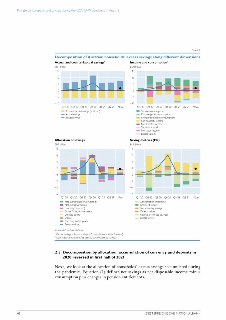
Private consumption and savings during the COVID-19 pandemic in Austria
48 OESTERREICHISCHE NATIONALBANK
2.3 Decomposition by allocation: accumulation of currency and deposits in 2020 reversed in first half of 2021
Next, we look at the allocation of households’ excess savings accumulated during the pandemic. Equation (1) defines net savings as net disposable income minus consumption plus changes in pension entitlements.
EUR billion
Actual and counterfactual savings1
15
10
5
0
−5
−10
EUR billion
Income and consumption2
15
10
5
0
−5
−10
Decomposition of Austrian households' excess savings along different dimensions
Chart 1
Source: Authors’ calculations.1 Excess savings = Actual savings – Counterfactual savings (inverted).2 A fall in consumption implies positive contributions to savings.
Counterfactual savings (inverted)Actual savingsExcess savings
Services consumptionDurable goods consumptionNondurable goods consumptionNet property incomeNet transfer incomeShort-time workNet labor incomeExcess savings
EUR billion
Allocation of savings
8
6
4
2
0
−2
−4
−6
EUR billion
Saving motives (M0)
8
6
4
2
0
−2
−4
−6
Net capital transfers (inverted)Net capital formationFinancing (inverted)Other financial investmentUnlisted equitySharesCurrency and depositsExcess savings
Consumption smoothingIncome structurePrecautionary savingsOther motivesResidual (= forced savings)Excess savings
Q1 20 Q2 20 Q3 20 Q4 20 Q1 21 Q2 21 Mean Q1 20 Q2 20 Q3 20 Q4 20 Q1 21 Q2 21 Mean
Q1 20 Q2 20 Q3 20 Q4 20 Q1 21 Q2 21 MeanQ1 20 Q2 20 Q3 20 Q4 20 Q1 21 Q2 21 Mean

Private consumption and savings during the COVID-19 pandemic in Austria
MONETARY POLICY & THE ECONOMY Q4/21 49
Net savings (B.8n) = A net disposable income – consumption + + changes in pension entitlements (D8)
(1)5
Besides savings, total funds available for nonconsumption purposes ( = investment) include net wealth transfers and net financing (left-hand side of equation (2)). Households can use these funds to invest in real assets (net capital formation) or in financial assets.
Savings (B.8n) + net wealth transfers (D9.r – D9.p) + net financing (F.LIAB) = = net capital formation (P.5g – P.51c) + financial investment (F.ASSETS) (2)
If we rearrange equation (2), we can obtain the allocation of savings by equation (3):
Savings (B.8n) = net capital formation (P.5g – P.51c) + + financial investment (F.ASSETS) – net wealth transfers (D9.r – D9.p) – – net financing (F.LIAB)
(3)
Financial investment in the quarterly financial accounts comprises 17 different categories. To simplify our analysis, we aggregate these into four categories ( currency and deposits, shares, unlisted equity and other financial investment).
Our calculation of excess financial investment differs from that of excess savings. Since we did not produce forecasts for financial investment in the December 2019 Broad Macroeconomic Projection Exercise (BMPE) and since seasonal adjustment yields questionable results for some series, we calculate excess financial investment in the following way: For each category of financial investment, we first calculate the deviation of quarterly levels during the period from Q1 20 to Q2 21 from the respective average quarterly level for the years from 2017 to 2019 and then rescale it, so that excess financial investment plus excess real investment match total excess funds available.
The bottom left-hand panel of chart 1 shows the results of this decomposition. On average over the six quarters under observation, all components of excess savings show similar contributions to households’ total savings. Over time, a distinct profile emerges. During the first lockdown in Austria (Q1 20), house-holds’ excess savings were mostly used to invest in unlisted equity, i.e. to support households’ own businesses classified in the household sector. In the second half of 2020, the bulk of excess savings were used for the accumulation of currency and deposits, whereas in the first half of 2021, the decline in the savings ratio was driven by the reduction of this position. Other financial investment played a dominant role in the buildup of savings in Q1 20 and in their reduction in Q3 20, while shares only played a minor role.
2.4 Decomposition by motive: increase of savings ratio driven by forced savings
Next, we decompose households’ total actual savings into saving motives. We do this by econometrically estimating various models for the savings ratio. The variables used in these models try to capture the following standard motives and/
5 National account codes in parantheses.

Private consumption and savings during the COVID-19 pandemic in Austria
50 OESTERREICHISCHE NATIONALBANK
or determinants of saving: consumption smoothing, the composition of income, precautionary savings, Ricardian savings and a savings target. In addition to these motives, we include the real interest rate and the debt-to-income ratio in our analysis as controls.6 The residual of these estimations during the pandemic will be interpreted as “forced” savings (in line with Dossche and Zlatanos, 2020), i.e. as consumption that could not materialize due to business shutdowns (mostly services).
First, we consider consumption smoothing, which is a direct consequence of the permanent income hypothesis (Friedman, 1957) and the life cycle hypothesis (Modigliani and Brumberg, 1956). The permanent income hypothesis states that current consumption depends on expected long-term permanent income and not on current income, as suggested by Keynesian theory. According to the life cycle hypothesis (Modigliani, 1956), households want to maintain a stable consumption path over their entire lifetime. Both theories imply that savings increase in periods with higher income and decrease in periods with lower income. Our proxy for consumption smoothing is the percentage deviation of real disposable household income from the quarterly sectoral accounts from its trend.7 In periods when disposable income is above (below) its trend, savings should increase (decrease); thus, we expect the respective coefficient to have a positive sign.
Our second determinant is the composition of income. Empirical literature8 shows that the marginal propensity to consume (MPC) differs considerably across income components. The MPC is defined as the amount of additional consumption generated by one additional unit of income and/or wealth. De Bondt et al. (2019) reviewed the empirical literature and estimated MPCs for the euro area and its four largest economies (Germany, France, Italy, Spain). They distinguish between labor income, transfer income, property income, financial wealth and nonfinancial (housing) wealth. The bulk of estimates for the MPC out of labor and transfer income ranges from 0.8 to 1, whereas the MPC out of property income is much lower in most cases (0.07 to 0.3). The estimates for the MPC out of wealth are substantially lower, between 0 and 0.01.9 According to our own estimates for Austria (see annex 3, table A1), the MPC for nonproperty income is always higher (0.75 to 1.05) than that for property income (0.54 to 0.71).10 Our proxy variable for income composition is the share of net property income in total (net) disposable household income. Net labor income, net transfer income and net property income are calculated from quarterly sectoral accounts data.11 On aggregate, a higher share of income from property should, ceteris paribus, lower consumption and thus
6 Besides the motives used in our models, there are other saving motives such as, i.a., bequest (Kotlikoff, 1988, or Dynan, Skinner and Zeldes, 2002), imperfect capital markets (Liu and Woo, 1994) or buffer stock savings (Carroll, 1997).
7 We calculate the trend employing an HP filter.8 See e.g. Winkler (2016), Rodriguez-Palenzuela et al. (2016) or de Bondt et al. (2019). 9 See Fenz and Fessler (2008) for a review of the empirical literature before the financial crisis.10 These macroeconomic MPCs for Austria were obtained by estimating the long-run equilibrium relationship between
private consumption, labor income, transfer income, property income, net financial wealth and housing wealth for the period from Q1 01 to Q4 19 in seven private consumption models. All variables were entered in real terms and logs. We found stable cointegrating relationships between the variables. In the specifications with only two income components, the MPC for nonproperty income (0.75 to 1.05) is larger than that for property income (0.54 to 0.71). In models with three income components, the results are mixed (see annex 3, table A1).
11 Since the sectoral accounts only record total direct taxes and social security contributions paid by the household sector, total direct taxes were disaggregated into the three income categories using tax data.

Private consumption and savings during the COVID-19 pandemic in Austria
MONETARY POLICY & THE ECONOMY Q4/21 51
increase savings. Hence, we expect the coefficient of income composition to have a positive sign.
Third, we consider the precautionary savings motive. The theory of precautionary savings states that uncertainty about future income developments triggers the accumulation of wealth. Although this hypothesis has been tested in many studies, empirical results are not conclusive about the prevalence of precautionary savings and the best proxy variables for empirical work (Lugilde et al., 2017). Kennickell and Lusardi (2005) found that the role of precautionary savings is low, at an aggregate level, for the USA. Desired precautionary wealth accounts for only 8% of households’ total net worth and is mainly accumulated by older households and business owners. We use two proxies, namely “adequate for savings” from the European Commission’s business and consumer survey (“the current economic situation is adequate for savings”) and unemployment expectations (“How do you expect the number of people unemployed in this country to change over the next 12 months?”, quoted in Dossche and Zlatanos, 2020) from the same source. Assuming that consumers find it more adequate to save and expect higher future unemployment in periods of high individual or general economic uncertainty, an increase in these proxy variables should be associated with higher savings; thus, we expect both coefficients to have a positive sign.
Fourth, we look at the role of Ricardian savings. According to Ricardian theory, additional government transfers or tax reliefs to households do not increase consumption because forward-looking households end up saving all their additional income from these transfers or reliefs since they expect future tax increases to pay the deficits incurred at present. It is a well-known stylized fact that Ricardian equivalence in its purest from rarely holds in practice. Recently, Armantier et al. (2020) and Baker et al. (2020) investigated the impact of US government support to households during the pandemic. They found that between 25% and 40% of these funds were spent, indicating Ricardian equivalence only to some degree. We use the year-on-year absolute difference of the government debt-to-GDP ratio from the quarterly national accounts as a proxy for the Ricardian savings motive. An increasing government debt-to-GDP ratio may signal a future need for budget consolidation, i.e. tax increases, which according to Ricardian theory should lower consumption and thus increase savings in the present period. Thus, we expect the coefficient attached to this proxy variable to have a positive sign.
Fifth, the savings target addresses the role of wealth in saving decisions. The buffer stock savings theory postulates that households have a certain stock of savings that they target. If their target wealth falls below this target, they increase their savings, and vice versa. We use three different variables for financial wealth, namely the total wealth-to income-ratio, the net financial wealth-to-income ratio and the real (housing) wealth-to-income ratio (see footnote 10 for details on the calculation of the wealth variables). These variables capture different aspects of wealth, with the intuition that, on aggregate, increasing wealth should enable more households to reach their savings target and thus decrease their savings related to this motive. Therefore, we expect negative coefficients on these three proxy variables.
Finally, we include two additional variables: the real interest rate and the debt-to-income ratio. The real interest rate is an important determinant of saving decisions. In theory, higher interest rates make saving more attractive and should

Private consumption and savings during the COVID-19 pandemic in Austria
52 OESTERREICHISCHE NATIONALBANK
therefore drive up savings. In reality, additional other factors (“income effect”) are at play which render the relationship between interest rates and savings less clear.12 The empirical literature finds mixed evidence (see e.g. Elmendor, 1996, or Beznoska and Ochmann, 2013). We use the interest rate on consumer loans, deflated by annual HIPC inflation. The basic idea behind including the household debt-to-income ratio is that, in the national accounts, debt repayments are counted as savings. Higher debt would thus lead to higher savings, and including this variable should control for this accounting effect.
We estimate a full (general) model (M0) that includes all of the above- mentioned motives with their described proxy variables and serves as our bench-mark model in the decomposition by saving motives. Based on this general model, we estimate a set of submodels13 which focus on specific saving motives and also serve as robustness checks (M1 to M8). We limit the estimation sample to the period prior to the pandemic (Q1 01 to Q4 19). We include the lagged endogenous variable in all models to account for autocorrelated residuals. Table 2 shows the estimation results for our benchmark model (M0) and the eight different submodel specifications (M1 to M8). All coefficients have the expected sign in all models. There is only one insignificant variable, namely the total wealth-to-income ratio, in the general model. All other variables are significant, most of them at the 1% level.
Consumption smoothing and income composition are included in all submodels. Compared with the benchmark model, the coefficient of consumption smoothing decreases in the submodels, whereas the coefficient of the income composition proxy variable increases. In specifications with proxies for precautionary savings (M0, M2, M3, M5), the coefficient of the share of property income is lower (0.20 to 0.26) than in specifications without this determinant (0.30 to 0.41). Precautionary savings hence reduce the explanatory power of the property income share. This result supports the findings of Kennickell and Lusardi (2005), who found that precautionary savings are mainly accumulated by older households and business owners. Since our measure of property income includes the net operating surplus of businesses that are part of the household sector, our proxy variables for precau-tionary savings and income composition partially overlap.
Ricardian effects are significant in the benchmark model (M0) and two submodels (M4, M5). The coefficients of our proxy variables for the savings target show the expected negative sign and are significant in submodels M6 to M8. In the general model, the coefficient is considerably lower and not significant. The effects of the debt-to-income ratio and the lending rate are also somewhat lower in our fully specified benchmark model (M0) than in the two submodels in focus (M1, M3).
Chart 2 shows the individual models’ in-sample and out-of-sample predictions of the savings ratio. The left-hand panel shows the fitted values of the savings ratio in the benchmark model (M0) and the eight submodels (M1 to M10) together with the actual values over the estimation horizon. All specifications capture the historical
12 When interest rates rise, forward-looking households will anticipate their income to rise since higher interest rates signal higher growth expectations (Dirschmid and Glatzer, 2004). Households that post high shares of interest income might increase their savings when interest rates increase.
13 The submodels were estimated using a specific-to-general approach, starting with the variable(s) in focus and keeping added variables only if they were statistically significant and did not render the variable(s) in focus statistically insignificant.
Table 3
Estimation results of the savings ratio equations
M01 M1 M2 M3 M4 M5 M6 M7 M8
CoefficientsConstant –3.05 –3.03 0.36 –5.38 –2.13 0.58 4.11 2.66 4.35Lagged dependent variableT–1 0.02 0.38 ***T–2 0.26 *** 0.27 *** 0.26 *** 0.36 *** 0.37* 0.36 ***Consumption smoothingTrend deviation of disposable income 0.70 *** 0.36 *** 0.40 *** 0.43 *** 0.35 *** 0.39 *** 0.36 *** 0.37 *** 0.35 ***Income compositionShare of property income in total income 0.20 *** 0.41 *** 0.24 *** 0.22 *** 0.39 *** 0.26 *** 0.31 *** 0.33 *** 0.30 ***Precautionary savingsConsumer survey (“save now”) 0.05 *** 0.03 *** 0.07 *** 0.03 ***Unemployment expectations 0.01 ** 0.01 ** 0.02 ***Ricardian savingsGovernment debt-to-GDP ratio 0.06 *** 0.06 ** 0.06 ***Savings targetTotal wealth-to-income ratio –0.19 –0.80 **Net financial wealth-to-income ratio –1.68 **Housing wealth-to-income ratio –1.33 *Other variablesDebt-to-income ratio 0.07 *** 0.09 ***Lending rate 0.19 ** 0.40 ***R2 0.95 0.86 0.85 0.84 0.82 0.86 0.82 0.83 0.82Durbin-Watson statistic 1.93 2.09 2.07 2.06 2.14 1.92 1.89 1.92 1.86
Source: Authors’ calculations.1 M0 = benchmark model; M1 to M8 = submodels.

Private consumption and savings during the COVID-19 pandemic in Austria
MONETARY POLICY & THE ECONOMY Q4/21 53
development of the savings ratio well. The middle panel of chart 2 shows the conditional forecasts of the savings ratio with the realized values of the conditioning variables for the period from Q1 19 to Q2 21. For Q1 20 to Q2 21, these forecasts are out of sample. None of the specifications come close to predicting the observed path of the savings ratio; instead, they predict a sharp decline for Q2 20, when, in fact, the savings ratio was already increasing. The subsequent movements of the savings ratio (increase until Q4 20, fall afterward) are predicted correctly (regarding the direction) but the predicted level of the savings ratio remains too low.
The right-hand panel of chart 2 shows a decomposition into saving motives of the excess savings Austrian households accumulated during the pandemic (EUR 10.8 billion) for each of our nine models (see also table A2). Although the impor-tance of the individual motives differs between specifications, the main result is robust: The fall in disposable household income and the even stronger decline in property income combined with the role of consumption smoothing suggest that the savings ratio decreased instead of increased during the pandemic. The effect of precautionary savings on the savings ratio is positive but small. This might be an effect of the short-time work scheme, which reduced unemployment expectations considerably. Consequently, forced savings (defined as the residual) substantially
therefore drive up savings. In reality, additional other factors (“income effect”) are at play which render the relationship between interest rates and savings less clear.12 The empirical literature finds mixed evidence (see e.g. Elmendor, 1996, or Beznoska and Ochmann, 2013). We use the interest rate on consumer loans, deflated by annual HIPC inflation. The basic idea behind including the household debt-to-income ratio is that, in the national accounts, debt repayments are counted as savings. Higher debt would thus lead to higher savings, and including this variable should control for this accounting effect.
We estimate a full (general) model (M0) that includes all of the above- mentioned motives with their described proxy variables and serves as our bench-mark model in the decomposition by saving motives. Based on this general model, we estimate a set of submodels13 which focus on specific saving motives and also serve as robustness checks (M1 to M8). We limit the estimation sample to the period prior to the pandemic (Q1 01 to Q4 19). We include the lagged endogenous variable in all models to account for autocorrelated residuals. Table 2 shows the estimation results for our benchmark model (M0) and the eight different submodel specifications (M1 to M8). All coefficients have the expected sign in all models. There is only one insignificant variable, namely the total wealth-to-income ratio, in the general model. All other variables are significant, most of them at the 1% level.
Consumption smoothing and income composition are included in all submodels. Compared with the benchmark model, the coefficient of consumption smoothing decreases in the submodels, whereas the coefficient of the income composition proxy variable increases. In specifications with proxies for precautionary savings (M0, M2, M3, M5), the coefficient of the share of property income is lower (0.20 to 0.26) than in specifications without this determinant (0.30 to 0.41). Precautionary savings hence reduce the explanatory power of the property income share. This result supports the findings of Kennickell and Lusardi (2005), who found that precautionary savings are mainly accumulated by older households and business owners. Since our measure of property income includes the net operating surplus of businesses that are part of the household sector, our proxy variables for precau-tionary savings and income composition partially overlap.
Ricardian effects are significant in the benchmark model (M0) and two submodels (M4, M5). The coefficients of our proxy variables for the savings target show the expected negative sign and are significant in submodels M6 to M8. In the general model, the coefficient is considerably lower and not significant. The effects of the debt-to-income ratio and the lending rate are also somewhat lower in our fully specified benchmark model (M0) than in the two submodels in focus (M1, M3).
Chart 2 shows the individual models’ in-sample and out-of-sample predictions of the savings ratio. The left-hand panel shows the fitted values of the savings ratio in the benchmark model (M0) and the eight submodels (M1 to M10) together with the actual values over the estimation horizon. All specifications capture the historical
12 When interest rates rise, forward-looking households will anticipate their income to rise since higher interest rates signal higher growth expectations (Dirschmid and Glatzer, 2004). Households that post high shares of interest income might increase their savings when interest rates increase.
13 The submodels were estimated using a specific-to-general approach, starting with the variable(s) in focus and keeping added variables only if they were statistically significant and did not render the variable(s) in focus statistically insignificant.
Table 3
Estimation results of the savings ratio equations
M01 M1 M2 M3 M4 M5 M6 M7 M8
CoefficientsConstant –3.05 –3.03 0.36 –5.38 –2.13 0.58 4.11 2.66 4.35Lagged dependent variableT–1 0.02 0.38 ***T–2 0.26 *** 0.27 *** 0.26 *** 0.36 *** 0.37* 0.36 ***Consumption smoothingTrend deviation of disposable income 0.70 *** 0.36 *** 0.40 *** 0.43 *** 0.35 *** 0.39 *** 0.36 *** 0.37 *** 0.35 ***Income compositionShare of property income in total income 0.20 *** 0.41 *** 0.24 *** 0.22 *** 0.39 *** 0.26 *** 0.31 *** 0.33 *** 0.30 ***Precautionary savingsConsumer survey (“save now”) 0.05 *** 0.03 *** 0.07 *** 0.03 ***Unemployment expectations 0.01 ** 0.01 ** 0.02 ***Ricardian savingsGovernment debt-to-GDP ratio 0.06 *** 0.06 ** 0.06 ***Savings targetTotal wealth-to-income ratio –0.19 –0.80 **Net financial wealth-to-income ratio –1.68 **Housing wealth-to-income ratio –1.33 *Other variablesDebt-to-income ratio 0.07 *** 0.09 ***Lending rate 0.19 ** 0.40 ***R2 0.95 0.86 0.85 0.84 0.82 0.86 0.82 0.83 0.82Durbin-Watson statistic 1.93 2.09 2.07 2.06 2.14 1.92 1.89 1.92 1.86
Source: Authors’ calculations.1 M0 = benchmark model; M1 to M8 = submodels.

Private consumption and savings during the COVID-19 pandemic in Austria
54 OESTERREICHISCHE NATIONALBANK
contributed to the increase in the savings ratio.14 Our estimates of the different specifications for forced savings range from EUR 17 billion to EUR 23 billion ( accumulated over the period from Q1 20 to Q2 21). Specifications including the precautionary savings motive (our benchmark M0 and submodels M2, M3, M5) exhibit lower forced savings. The quarterly results of this decomposition for our benchmark model M0 can be found in the bottom right-hand panel of chart 1.
3 Implications for future consumption and saving patternsWhen looking at the expected development of household savings in Austria after the pandemic, we must distinguish between two different questions: First, how fast will the marginal propensity to save (MPS) out of current income go back to normal? And second, to what extend will the stock of excess savings accumulated
14 This result is in line with a similar exercise carried out in Dossche and Zlatanos (2020) for the euro area. It is also confirmed by the Deutsche Bundesbank’s Panel on Household Finances (PHF) survey of March 2021, in which half of the respondents indicated that over the past year they had more monetary resources available at the end of each month than before the pandemic. Of these 50%, which correspond to higher-income households, 95% reported that limited consumption opportunities were an important reason for their higher savings (Deutsche Bundesbank, 2021).
Savings ratio in %
Actual and fitted savings ratios, Q1 01 to Q4 19
16
14
12
10
8
6
4
30
25
20
15
10
5
0
−5
−10
−15
20
18
16
14
12
10
8
6
4
2
0
−2
Estimation results of the savings ratio equations: M0 to M81
Chart 2
Source: Authors’ calculations.1 M0 = benchmark model; M1 to M8 = submodels.
Savings ratio, net M0M1 M2M3 M4M5 M6M7 M8
Savings ratio, net ConstantInertiaConsumption smoothingIncome structurePrecautionary savingsRicardian savingsSavings targetOther variablesResidual ( = forced savings)Excess savings
M0M1 M2M3 M4M5 M6M7 M8
Q1 01 Q1 04 Q1 07 Q1 10 Q1 13 Q1 16 Q1 19 M0 M1 M2 M3 M4 M5 M6 M7 M8Q1 19 Q3 19 Q1 20 Q3 20 Q1 21

Private consumption and savings during the COVID-19 pandemic in Austria
MONETARY POLICY & THE ECONOMY Q4/21 55
during the pandemic be dissaved? The actual development of the savings ratio is the sum of these two effects. When households use their accumulated savings to satisfy pent-up demand, the observed savings ratio is below the MPS.
There is a consensus among most forecasters that the MPS will quickly decline as soon as all lockdown measures are lifted (see e.g. Deutsche Bundesbank, 2021; Banque de France, 2021; European Commission, 2021; or OECD, 2021). In the first half of 2021, savings in Austria almost reverted to pre-pandemic levels. How-ever, this was not due to the release of pent-up demand but to a decline in income, notably property income. Household consumption in Austria declined in the first quarter of 2021 due to the second lockdown and recovered in the second quarter of 2021 as containment measures were lifted. All components of private consump-tion were still below pre-crisis levels in Q2 21 except for durable goods, which were 24% above the level recorded in Q4 19.
There is a lot more disagreement in the literature regarding the amount or share of excess savings that will be spent to meet pent-up demand, however. Early evidence from Germany (Bernard, Tzamourani and Weber, 2020) suggests that consumers were significantly more cautious in their spending intentions after the relaxation of the first pandemic-induced lockdown in 2020. To shed light on this question, we focus on two different perspectives. First, we consider information from surveys asking households how they plan to use their excess savings. The available surveys exhibit a huge variation, depending on their timing and design and on country characteristics. They point toward some pent-up demand, which is of apparently limited magnitude, however.15 This is mainly because the lion’s share of excess savings is expected to have accrued in high-income households, which saw a strong increase in their savings during the pandemic while lower-income households did not increase their savings by much or even drew on existing savings. On average, one-quarter to one-third of excess savings is expected to be consumed. There is little information on the transition dynamics, i.e. the length of the period until this pent-up demand is satisfied, and on the respective spending profile over time.
Second, we draw on theoretical and empirical studies on households’ MPC out of savings. The MPC out of wealth is considerably lower than the MPC out of income (Albacete and Lindner, 2017; Jappelli and Pistaferri, 2014). The main problem with this approach, therefore, is whether households perceive their excess savings as additional income or as wealth. During the pandemic, most additional savings were accumulated by high-income households, which may have a higher tendency to perceive these excess savings as additional wealth. Some low-income households, by contrast, were unable to accumulate excess savings during the
15 In the Deutsche Bundesbank’s Panel on Household Finances (PHF) of March 2021, 70% of respondents indicated that they would spend part of their excess savings to consume goods and services once restrictions are lifted. Based on these responses, the Deutsche Bundesbank forecasts a lower bound of 25% of excess savings spent for consumption and an upper bound of 45%, with the baseline being 35% over the coming years (Deutsche Bundesbank, 2021). In a household survey conducted by the Bank of England, most households (about 70%) said they planned to hold their savings in their bank accounts, while only 10% of those households that had increased their savings (less than 3% of the whole sample) planned to spend the money they had saved (Bank of England, 2020). The Centre for Economics and Business Research (CEBR) asked 4,000 UK households about their future spending plans: 18% of households with increased savings plan to spend all excess savings in 2021, 33% plan to spend them partially and 38% do not plan to spend any of the savings in 2021. Overall, UK households said they planned to spend 26% of their aggregate savings in 2021.

Private consumption and savings during the COVID-19 pandemic in Austria
56 OESTERREICHISCHE NATIONALBANK
pandemic; they even incurred higher debts (Raja, 2021). Hence, it is reasonable to assume that their spending on pent-up demand after the pandemic will be limited and that a large share of excess savings will not be spent.
If we assume that 25% of excess savings (EUR 2.7 billion) will be spent on pent-up demand, this will result in a cumulated increase in Austrian GDP of EUR 2.4 billion (or 0.4%) until 2023 according to a simulation performed with the OeNB’s macroeconomic model (Austrian Quarterly Model – AQM). This assess-ment is, of course, subject to considerable uncertainty about the course of the pandemic and the consumption components16 that will be most affected.The medium- to long-term impact of the pandemic on consumer spending and saving is ambiguous. After a phase of higher consumption in reaction to pent-up demand, precautionary savings might increase, driven by the pandemic experience. This effect could last longer, as younger households have been heavily affected. In the long run, households’ higher saving rate might translate into higher invest-ment, which could improve productivity and potential output.
ReferencesAlbacete, N. and P. Lindner. 2017. How Strong is the Wealth Channel of Monetary Policy
Transmission? A Microeconometric Evaluation for Austria. In: Monetary Policy & the Economy Q2/17. OeNB.
Armantier, O., L. Goldman, G. Koşar, J. Lu, R. Pomerantz and W. van der Klaauw. 2020. How Have Households Used Their Stimulus Payments and How Would They Spend the Next? Liberty Street Economics, 13 October.
Baker, S., R. A. Farrokhnia, M. Pagel, S. Meyer, and C. Yannelis. 2020. Income, liquidity, and the consumption response to the COVID-19 pandemic and economic stimulus payments, VoxEU.org, 17 June. (https://voxeu.org/article/covid-19-fiscal-stimulus-measures-and-household-spending-us).
Bank of England. 2020. How has Covid affected household savings? https://www.bankofengland.co.uk/bank-overground/2020/how-has-covid-affected-household-savings.
Bernard, R., Tzamourani, P. and M. Weber 2020. How are households’ consumption plans affected by the COVID-19 pandemic? Deutsche Bundesbank. Research Brief 35th edition. November.
Beznoska, M. and Ochmann R. 2013. The interest elasticity of household savings: a structural approach with German micro data. Empir Econ 45. 371–399. https://doi.org/10.1007/s00181-012-0626-9
Carroll, C. D. 1997. Buffer-Stock Saving and the Life Cycle/Permanent Income Hypothesis. In: The Quarterly Journal of Economics 112(1). 1–55. http://www.jstor.org/stable/2951275
Centre for Economics and Business Research. 2021. Household saving and spending in the age of the coronavirus. A Cebr report for Scottish Friendly.
Deutsche Bundesbank. 2021. Perspektiven der deutschen Wirtschaft für die Jahre 2021 bis 2023. Monatsbericht Juni 2021.15−39.
16 Pent-up demand might be skewed toward holidays abroad. A survey conducted among UK households (Centre for Economics and Business Research, 2021) shows that 34% of households plan to spend their savings on holidays abroad and 28% plan to spend them on domestic holidays. Expenses for visits to restaurants and cafés rank third (28%) and expenses for food and drink fourth (25%). If we apply these results to Austria, we must consider the fact that Austrian residents’ domestic tourism expenditure was considerably above the pre-crisis level in the summers of 2020 and 2021. This implies that for the 2022 summer season, Austrians’ tourism-related pent-up demand will likely be skewed toward tourism abroad. On the other hand, it can be expected that the Austrian tourism sector will benefit from the release of pent-up demand from abroad.
Private consumption and savings during the COVID-19 pandemic in Austria
MONETARY POLICY & THE ECONOMY Q4/21 57
Dossche, M. and S. Zlatanos. 2020. COVID-19 and the increase in household savings: precau-tionary or forced? ECB Economic Bulletin, Issue 6 / 2020. 65−69.
Dynan, K .E., J. Skinner and S. P. Zeldes. 2002. The Importance of Bequests and Life-Cycle Saving in Capital Accumulation: A New Answer. In: American Economic Review 92 (2). 274−278.
European Commission. 2021. European Economic Forecast – Spring 2021. Institutional Paper 149. DG Economic and Financial Affairs. Luxembourg: Publications Office of the European Union. doi:10.2765/66679.
Elmendorf, D. 1996. The Effect of interes rate changes on household savings and consumption: A survey. Federal Reserve. http://www.federalreserve.gov/pubs/feds/1996/199627/199627pap.pdf
Fenz, G. and P. Fessler. 2008. Wealth effects on consumption in Austria. Monetary Policy & the Economy Q4/08. 68−84.
Fenz, G. and M. Schneider. 2012. Weak global trade darkens growth outlook for Austria. Economic outlook for Austria from 2019 to 2022. Monetary Policy & the Economy Q4/19. 10−39.
Kennickell, A. and A. Lusardi. 2005. Disentangling the importance of the precautionary saving motive. Mimeo. https://www.federalreserve.gov/econresdata/scf/files/precautionarynov052.pdf
Kotlikoff, L. J. 1988. Intergenerational Transfers and Saving. In: Journal of Economic Perspectives. Spring 1988.2(2). 41–45.
Liu, L.-Y. and W. T. Woo. 1994. Saving Behaviour Under Imperfect Financial Markets and the Current Account Consequences. In: The Economic Journal 104(424). 512–527. https://doi.org/10.2307/2234628
Lugilde, A., R. Bande and D. Riviero. 2017. Precautionary saving: a review of the theory and the evidence. MPRA Paper 77511.
Modigliani, F. and R. Brumberg. 1954. Utility analysis and the consumption function: an inter-pretation of cross-section data. In: Kurihara, K. (ed.). Post-Keynesian Economics. New Brunswick: Rutgers University Press. 388−436.
OECD. 2021. OECD Economic Outlook. Volume 2021. Issue 1. No. 109. OECD Publishing. Paris. https://doi.org/10.1787/edfbca02-en
Rodriguez-Palenzuela, D., S. Dees (eds.) and the Saving and Investment Task Force 2016. Savings and investment behaviour in the euro area. ECB Occasional paper 167.
Wiesinger S. 2021. Aktuelle Entwicklungen im Jahr 2020. Sonderheft STATISTIKEN Daten & Analysen. OeNB. Einkommen, Konsum und Vermögen der Haushalte – Sektorale Volks-wirtschaftliche Gesamtrechnungen in den letzten 20 Jahren. 5–7.
Winkler, S. 2016. Empirical Evidence of the Housing Wealth Effect. Available at SSRN: https://ssrn.com/abstract=2695778 or http://dx.doi.org/10.2139/ssrn.2695778

Private consumption and savings during the COVID-19 pandemic in Austria
58 OESTERREICHISCHE NATIONALBANK
Annex 1
Definition of the counterfactual scenario
As the basis for our counterfactual scenario, we use the OeNB’s last economic outlook for Austria that was produced prior to the pandemic for the Broad Macro-economic Projection Exercise (BMPE), i.e. the economic outlook of December 2019 (Fenz and Schneider, 2020). Since the level of historical data has been revised for most variables since then, and because of a forecasting error for Q4 19 (for sectoral accounts data also for Q3 19), we cannot directly use the level of the variable projected in December 2019 in this exercise. Instead, we extrapolate the historical data of Q4 19 with the quarterly growth rates calculated in the December 2019 BMPE for Q1 20 to Q2 21. Since not all variables needed for our exercise, e.g. financial investment, were projected in the BMPE, we had to forecast these variables on the basis of information that was available in December 2019. The components of private consumption were projected using the growth rate of total consumption from the December 2019 BMPE; financial investment and its components were projected using the growth rate of savings. Confidence indicators needed for the savings rate models were interpolated using the average value for 2019.
Annex 2
Income decomposition
In the quarterly nonfinancial sector accounts, disposable household income (according to the expenditure concept) is available for the following components: compensation of employees, mixed income, gross operating surplus, property income (interest income, other property income) and social transfers.
We follow de Bondt et al. (2019) and define the following three income categories17: Labor income is the sum of compensation of employees (D1R) and gross mixed income (B3G); transfer income is social benefits other than social transfers in kind (D62) plus other current transfers (D7); and property income is the sum of gross operating surplus (B2G, which consists mostly of imputed rents for owner- occupied housing) and net property income (D4, i.e. net interest earnings plus net other property income). However, our approach differs in the way how direct taxes (D5P) and social security contributions (D61) are distributed across these three income categories. While de Bondt et al. (2019) subtract social security contributions from labor income and distribute direct taxes proportion-ally among the income components, we use administrative tax data to distribute direct taxes among income components. This approach results in a much better estimate for income components after taxes, since the approach used by de Bondt et al. (2019) underestimates net property income. The main reasons for this under-estimation are that de Bondt et al. (2019) consider financial intermediation services indirectly measured (FISIM), i.e. imputed interest payments, and imputed rents for owner- occupied housing, which are not taxed, and the fact that dividend pay-ments in the national accounts are too high when compared with other statistics.
17 National accounts codes are given in parentheses.

Private consumption and savings during the COVID-19 pandemic in Austria
MONETARY POLICY & THE ECONOMY Q4/21 59
Annex 3
Table A1
Estimation results of the private consumption models1
C14 C2 C3 C4 C5 C6 C7
Elasticities2
Labor + transfer income 0.92 *** 0.72 *** 0.65 *** 0.67 ***Labor income 0.54 *** 0.29 *** 0.27 ***Transfer income 0.42 *** 0.41 *** 0.34 ***Property income 0.10 *** 0.12 *** 0.13 *** 0.13 *** 0.13 *** 0.15 *** 0.16 ***Total wealth 0.14 *** 0.18 ***Net financial wealth –0.06 * –0.09 **Housing wealth 0.25 *** 0.18 *** 0.32 ***Marginal propensity to consume3
Labor + transfer income 1.05 0.83 0.75 0.77Labor income 0.97 0.51 0.49Transfer income 1.31 1.27 1.08Property income 0.54 0.65 0.71 0.70 0.66 0.78 0.83Total wealth 0.01 0.01Net financial wealth –0.01 0.00Housing wealth 0.01 0.01 0.02
Source: Authors’ calculations.1 All variables are real and expressed in logs. We report only equations with signif icant estimation results.2 = percentage change of private consumption per 1% change of respective variable.3 = change of private consumption in euro per EUR 1 change in respective variable.4 C1 to C7 denote the seven different private consumption models estimated in this exercise.
Table A2
Decomposition of excess savings into saving motives
M01 M1 M2 M3 M4 M5 M6 M7 M8
Contributions to accumulated excess savings in EUR million
Constant 0.6 0.6 –0.1 1.0 0.4 –0.1 –0.8 –0.5 –0.8 Inertia –0.4 –0.4 –0.7 –0.4 –0.5 –0.6 –0.5 Consumption smoothing –7.5 –3.9 –4.3 –4.6 –3.8 –4.2 –3.8 –3.9 –3.7 Income structure –4.2 –8.7 –5.2 –4.6 –8.2 –5.5 –6.5 –6.9 –6.4 Precautionary savings 2.0 1.4 2.6 0.8 Ricardian savings 2.0 1.8 1.9 Savings target –0.1 –0.3 –0.2 –0.4 Other variables 0.2 0.6 –0.1 Residual (= forced savings) 17.9 22.7 19.4 16.5 21.3 18.4 22.8 22.9 22.7 Excess savings 10.8 10.8 10.8 10.8 10.8 10.8 10.8 10.8 10.8
Source: Authors’ calculations.1 M0 = benchmark model; M1 to M8 = submodels.

MONETARY POLICY & THE ECONOMY Q4/21 61
A new instrument to measure wealth inequality: distributional wealth accounts
Arthur B. Kennickell, Peter Lindner, Martin Schürz1
Refereed by: Andrea Neri, Banca d’Italia
In this study we investigate the sensitivity of different wealth measurement approaches. In this context, we analyze the alignment of Household Finance and Consumption Survey (HFCS) data with national accounts data and examine the production of distributional wealth accounts, which poses severe conceptual challenges. For a number of reasons, household surveys under-estimate top wealth shares. We show that different assumptions generate a wide range of results for different wealth inequality indicators. In particular, the share of the top 1% of households in net wealth ranges from about 25% to about 50%, depending on the underlying assumption. Thus, while the true value of the wealth share held by the top 1% is unknown, all available information indicates that it is closer to 50% than to HFCS results. We call for caution in interpreting top shares as the underlying assumptions are mostly ad hoc choices made by data producers. Our study argues that we need better microdata on the top end of the net wealth distribution.
JEL classification: C80, D30, D31, E01, E21Keywords: HFCS, national accounts, distribution, micro-macrodata integration
Wealth inequality has moved center stage in economic debates today – even at central banks.2 Thus, issues relating to wealth distribution measurement have become crucial. The well-known Stiglitz-Sen-Fitoussi Report (Stiglitz et al., 2009) already acknowledged the need for timely and adequate information on wealth inequality measurement. And for quite some time, various international institu-tions such as the Organisation for Economic Co-operation and Development (OECD), Eurostat, a number of research networks3 and Thomas Piketty’s World Inequality Database (WID)4 have undertaken extensive efforts to improve wealth inequality measurement (see e.g. Chancel, 2022). These efforts yield yearly, quarterly or even real-time data on the distribution of wealth stocks.
The financial accounts are part of the System of National Accounts. In the next few years, the financial accounts will include distributional wealth information to complement the aggregate statistics in several countries. Wealth inequality measurement would then be able to draw on information on wealth ownership
1 Stone Center, City University of New York, [email protected]; Oesterreichische Nationalbank, Economic Analysis Division, [email protected], [email protected] . Opinions expressed by the authors of studies do not necessarily reflect the official viewpoint of the OeNB or the Eurosystem. The authors would like to thank Pirmin Fessler, Stefan Humer, Franziska Disslbacher, Emanuel List, Severin Rapp, Matthias Schnetzer, Erza Aruqaj, Stefan Wiesinger and Nicolás Albacete for helpful comments and valuable suggestions. Additionally, the authors would like to acknowledge the contribution of the ESCB Expert Group on Linking Macro and Micro Data for the Household Sector as well as the ESCB Expert Group on Distributional Financial Accounts, on which most of the R code used in this analysis is based.
2 See e.g. the paper by Doepke et al. (2019) presented at the ECB conference “Money Macro Workshop” in 2019 and the speech given by ECB Executive Board member Yves Mersch in Zurich in 2014, available at www.ecb.europa.eu/press/key/date/2014/html/sp141017_1.en.html.
3 For more information, see https://ec.europa.eu/eurostat/web/experimental-statistics/income-consump-tion-and-wealth.
4 https://wid.world/.
A new instrument to measure wealth inequality: distributional wealth accounts
62 OESTERREICHISCHE NATIONALBANK
with respect to specific socioeconomic groups, such as breakdowns by profession or ownership status regarding a household’s main residence. The US Federal Reserve, for instance, already publishes distributional financial accounts – also as modern dashboards – on a regular basis.5
In this paper, we discuss the question of how reliable key statistics on distribu-tional wealth indicators are. In the case of Austria considered in this paper, we find an extremely wide range of estimates for key indicators, depending on the under-lying assumptions. We link micro- and macrodata on wealth and discuss various problems of the available data sources. We apply different procedures to correct for these problems. Essentially, we follow the literature (ECB, 2020) to generate distributional wealth accounts for Austria and assess the sensitivity of key results with respect to assumptions made during the estimation procedure.6 The goal of our analysis is to assess the impact potential of ad hoc assumptions on results which will, in turn, be used later. We refrain from any judgment on which simulation procedure is preferable. Our focus on Austria limits the specific results of our analysis, although the more conceptual points apply more broadly. Close inspection of the statistical variability of estimates, i.e. looking at standard errors and/or vari-ability due to imputation, sampling and estimation methods used, is left to future research.
In the EU, the quality of statistical data is regulated by the “Quality Assurance Framework of the European Statistical System.”7 According to this framework, the quality of statistical data is “measured by the extent to which the statistics are relevant, accurate and reliable, timely, coherent, comparable across regions and countries, and readily accessible by users, […]” (European Statistical System, 2019, p. 45). Our analysis only considers the question whether statistical data are accurate and reliable. Accuracy is determined by the closeness of an estimate and its true counterpart in reality. But as the true value of an indicator is not known in practice, this criterion cannot be assessed adequately. The impact of alternative assumptions on the resulting data provides information on the reliability of data points that are eventually published.
The actual magnitude of wealth inequality is unknown. Without an external reference to “true” wealth concentration, it is not possible to judge what kind of assumptions are more or less “plausible” (Mooslechner et al., 2004). Plausibility itself is in the eye of the beholder.
An accurate Global Asset Registry would make it possible to provide the missing wealth data. In addition, such a registry could be a tool against illicit financial flows. The European Commission is currently investigating the idea of an EU Asset Registry.8 A Global Asset Registry would centralize relevant information on assets owned by natural persons, thereby providing information on global wealth concentration and on whether wealth data correspond to income tax regis-ter data. These data would also allow for depicting distributional wealth accounts in the System of National Accounts without requiring an extensive estimation
5 www.federalreserve.gov/releases/z1/dataviz/dfa/.6 While we look at stocks recorded in the household balance sheet, the impact of modeling choices on flows such as
income is discussed in Humer et al. (2021).7 https://ec.europa.eu/eurostat/documents/64157/4392716/ESS-QAF-V2.0-final.pdf.8 www.brusselsreport.eu/2021/08/30/european-commission-investigates-the-idea-of-an-eu-asset-registry/.

A new instrument to measure wealth inequality: distributional wealth accounts
MONETARY POLICY & THE ECONOMY Q4/21 63
procedure, which is necessary if results are based on survey data alone. To be effective, such a registry would need to be fully global, with measures in place to ensure compliance.
This paper is structured as follows: Section 1 introduces the data used in our study. In section 2, we refer to the related literature and present the investigated problem. We also discuss different modeling approaches as well as a selection of important assumptions. Section 3 discusses the results and section 4 draws policy conclusions.
1 Data and data sourcesThis section introduces the various data sources underlying our study. First and foremost, we use information from the Household Finance and Consumption Survey (HFCS) and the national accounts (NA) for Austria. Administrative micro-data on wealth would improve our wealth estimates but such data do not exist in Austria, given that the wealth tax was abolished in 1994 and the inheritance tax in 2008. As capital income tax is deducted at the source, capital income tax information cannot be used, either. Moreover, because micro- and macrodata are constructed in different ways, it is important to consider how comparable the resulting data might be.
1.1 Household Finance and Consumption Survey (HFCS)
We use data from the third wave of the HFSC 2017 (www.hfcs.at) for Austria.9 As a euro area-wide project, the HFCS gathers information on households’ complete balance sheets, including detailed data on wealth, income, and expenditure, along with a rich set of socioeconomic variables. The unit of observation is the household.
The field period of the third wave ran from the end of 2016 until mid-2017 and comprised extensive quality checks, including the option to contact a household again to clarify details and/or correct deficiencies. About one-tenth of respondents (around 300 households) were recontacted to clarify or correct previously gath-ered information.
Missing information in the survey is multiply imputed, based on a chained Bayesian regression approach. Weighting ensures that the participating part of the gross sample represents the (targeted) household population in Austria along key demographic and geographic dimensions. Although the response rate in the Austrian HFCS 2017 is about 50% (see annex A, table A2), which is rather high compared with the rate observed in Germany and other countries, the observed sample is likely biased in ways that are not corrected by weighting adjustments. Furthermore, there is no oversampling of the affluent population in the Austrian HFCS 2017. A crucial difference between the set of survey participants and the overall population is the absence of very wealthy households in the HFCS.10
9 For the corresponding first results report, see Fessler et al. (2018), and for the methodological report containing the technical details, see Albacete et al. (2018).
10 The value of the net wealth of the most affluent household participating in the HFCS comes close to EUR 70 million (in one implicate). Furthermore, there are fewer than five observations in each implicate that are above EUR 10 million.

A new instrument to measure wealth inequality: distributional wealth accounts
64 OESTERREICHISCHE NATIONALBANK
1.2 National accounts (NA)
The System of National Accounts has been well established for more than a century. Its newest requirements are laid down in the European System of Accounts (ESA) 2010. In its publication “European system of accounts – ESA 2010,”11 the European Commission provides the details and definitions of the national accounts (NA). In this paper, we use NA data for Austria for Q1 17, which correspond to the middle of the field period of the HFCS data used.
I.3 Data alignment
In addition to aligning the reference periods of the two data sources (Q1 17), it is essential that the collected information and the definitions are comparable. The European Central Bank (ECB, 2020b) describes in detail the process of linking micro- and macrodata to produce distributional financial accounts and discusses the comparability of these data.12
Following the ECB’s approach, the net wealth concept applied in this study differs from that used in the HFCS. Moreover, it does not follow the definition of financial wealth given in the national accounts. First, cash holdings are estimated in the NA but are not measured in the HFCS. Money owed between households nets out conceptually in the NA (as long as the related transactions take place between households in one country) but is available at the individual household level in the HFCS. Thus, both items need to be excluded from a comparable wealth definition. Additionally, other real assets such as cars or collectibles (which are included in the HFCS net wealth definition) are not considered in this exercise because they are not included in the NA figures.
Thus, for our purposes, net wealth includes the following items:• deposits• bonds• shares• funds• entitlements from voluntary pension contributions• business wealth• housing wealth• mortgages and other liabilities
Moreover, the household sector as defined in the national accounts also includes nonprofit institutions serving households (NPISHs) such as churches (for part of the household balance sheet). This definition differs from what is economically understood as being a household, and it also differs from what is referred to as households in public discussion. Thus, whenever possible, we exclude NPISHs from the NA figures used here. It is important to note that this separation is not possible for land underlying dwellings on the real asset side of households’ balance sheets.13 People living in institutions such as homes for the elderly or prisons are excluded from the target population in the HFCS. This separation differs from the NA accounting unit, which considers the entire resident population.
11 Available at https://ec.europa.eu/eurostat/documents/3859598/5925693/KS-02-13-269-EN.PDF. pdf/44cd9d01-bc64-40e5-bd40-d17df0c69334?t=1414781932000 .
12 See also Andreasch and Lindner (2016), who show similarities and differences of micro- and macrodata.13 According to GEWINN (2019), 3 out of the 10 largest private holders of forests in Austria are monasteries.

A new instrument to measure wealth inequality: distributional wealth accounts
MONETARY POLICY & THE ECONOMY Q4/21 65
I.4 Other sources of information
The estimated totals derived from NA and HFCS data do not align well enough to support the straightforward joint usage of both data sources (see section 2.1). In particular, because HFCS estimates commonly fall short of NA estimates, we must look for other distributional information that may help address this shortfall. Additional information on the top tail of the wealth distribution may help improve the focus of the HFCS. To this end, we use information from several so-called rich lists and other sources, namely the following:
Forbes World’s Billionaires list
This list is published yearly and ranks US-dollar billionaires around the world. The documentation Forbes provides on the methodology of data production is mini-mal.14 Various estimations seem to be involved. Moreover, the fact that reported wealth is sometimes individual and sometimes aggregated across individuals makes correspondence to a household measure unclear. There are eight Austrians on the list, whose wealth ranges from USD 1.3 billion to USD 13.4 billion.15
Austrian rich list according to trend magazine
The Austrian business magazine trend publishes a list of the 100 richest Austrians,16 including wealth data (partly expressed in ranges). There is no publicly available documentation of the methods applied to generate this list. A variety of sources seem to be used to compile information on net wealth. Past values are updated by recent valuations using information on stock value and economic development. The list only partly covers wealth held abroad and it includes persons no longer residing in Austria. The magazine does not make any claims for data completeness or quality, as would be the case with official statistics.
Despite its deficiencies, this list is often used to discuss issues concerning the top of the wealth distribution as it is the only nationally published rich list for Austria. In 2017, it listed 100 persons or families whose wealth ranged from EUR 150 million to EUR 35.7 billion, including 40 billionaires. Adjusting these data to the appropriate household level is impossible. Moreover, a lot of persons are listed within relatively large wealth intervals, such as between EUR 150 million and EUR 600 million. Since we do not have any additional information, we assume the level of wealth could be adequately described by the midpoints of the ranges.
14 With regard to the methodology used, Forbes publishes the following information on its website Forbes Billionaires 2021: The Richest People in the World (accessed on March 4, 2021): “The Forbes World’s Billionaires list is a snapshot of wealth using stock prices and exchange rates from March 18, 2020. Some people become richer or poorer within days of publication. We list individuals rather than multigenerational families who share fortunes, though we include wealth belonging to a billionaire’s spouse and children if that person is the founder of the fortunes. In some cases, we list siblings or couples together if the ownership breakdown among them isn’t clear, but here an estimated net worth of USD 1 billion per person is needed to make the cut. We value a variety of assets, including private companies, real estate, art and more. We don’t pretend to know each billionaire’s private balance sheet (though some provide it). When documentation isn’t supplied or available, we discount fortunes.”
15 As an aside, one of the surprising facts about the Forbes World’s Billionaires list is that it does not contain billionaires from Luxembourg or Malta.
16 Information on the latest trend rich list is available at www.trend.at/wirtschaft/ranking-oesterreicher-10848600 (accessed on October 14, 2021).

A new instrument to measure wealth inequality: distributional wealth accounts
66 OESTERREICHISCHE NATIONALBANK
OeNB in-house information
The Oesterreichische Nationalbank (OeNB) maintains a variety of data for internal use. The information used in this paper covers about 150 affluent individuals and/or households in Austria whose net wealth is estimated to range between EUR 500 million and EUR 45 billion. Individuals can be mapped into households (i.e. whether they are living together or not) but net wealth held in shared ownership of a company cannot be split. These data can be used to assess the quality of the published rich lists and, potentially, to model the top of the wealth distribution in Austria.
The Austrian business register database Sabina
In addition to the data introduced above, we also rely on information derived from the Austrian business register database Sabina. With the data available there, it is possible to create a database of about 2,600 owners of companies other than stock companies with an average market value of about EUR 30 million (with valuations ranging from a minimum of EUR 5 million, i.e. the minimum imposed to be included in the list, to about EUR 2.3 billion, including six billionaires). The estimation of a company’s market value is based on the book value. A look-through approach to ownership records identifies the ultimate owner of a company, so that we can work with personal-level information instead of information at the level of individual companies. Double-counting of certain business assets is possible in the lists we use. Additionally, there are flaws as some companies are registered abroad. We do not claim that this is the best information available on companies. For us, this additional information solely serves as another example of a potential basis for modeling the top of the wealth distribution as introduced below.
2 Wealth measurement problemsThis section presents the basic problems of aligning micro- and macrodata and approaches on how to tackle them. In the process, we seek to document the reasons why these two measures may differ.
2.1 Coverage rates
To jointly analyze wealth survey and NA data in a meaningful way, both data sources should cover items that are conceptually the same, as discussed above. One of the main additional obstacles in generating national distributional wealth accounts, however, is the relatively low coverage rate of certain wealth compo-nents in wealth surveys compared to the NA.
Chart 1 shows the coverage rates for aggregates of selected financial wealth categories whose definitions in the HFCS and the NA are comparable.17 We see that the coverage rate varies substantially across financial instruments. In general, survey data tend to underestimate aggregate NA figures. However, aggregates derived from the survey can also be above 100% in relation to NA aggregates, e.g. for business wealth.18 Linking HFCS business wealth (non-self-employment private business and self-employment business) data to NA business wealth data (F512
17 Similar information can be found e.g. in ECB (2020b) or, for Austria, in Andreasch and Linder (2016).18 The sampling variability for the estimate of total business wealth may be rather high given the low number of
observations of relatively large wealth values.

A new instrument to measure wealth inequality: distributional wealth accounts
MONETARY POLICY & THE ECONOMY Q4/21 67
unlisted shares + F519 other equity + mainly nonfinancial assets) remains a key challenge.
Coverage rates in Austria (marked by the diamonds in chart 1) are comparable to those in other euro area countries.19 Thus, we expect the exercise below to yield similar results for other countries.
2.2 Discussion of potential problems
Depending on the reasons for the discrepancies in coverage noted above, the appropriate way to adjust information on wealth will vary. Among the principal sources that explain the differences between the micro- and macrodata described above are the following:
Missing the top
Based on the results presented in the literature (see e.g. Vermeulen, 2018), it seems that extreme wealth concentration at the top of the distribution explains a substan-tial fraction of the undercoverage shown above. We discuss this issue in greater
19 In Austria, life insurance contracts are considered a saving vehicle. For this reason, we aggregated the wealth categories and/or financial instruments F29 and F62 to make coverage rates more easily comparable across countries. See Fessler et al. (2018) for details on how information on life insurance contracts is collected in Austria. We only use data on endowment insurance contracts, i.e. contracts that provide for payout at the maturity date also in case the insured person is still alive.
Financial instruments
F22 – sight accounts
F29/F62 – savings/life insurance
F3 – bonds
F511 – shares
F51M – equity
F52 – funds
F4 – debt
Coverage of NA aggregates by HFCS aggregates
Chart 1
Source: HFCS 2020, ECB, national accounts and/or sector accounts for the middle of the reference period.
AT
Coverage rates in %0 50 100 150 200 250 300 350 400
Note: This chart shows the ratio of aggregates estimated from HFCS data to NA aggregates for 20 European countries. Austria is indicated by diamonds. Boxes are defined by the 25th and 75th percentiles, with the median indicated by a bar. The whiskers at the low (high) end indicate the lowest (highest) value above the 25th percentile minus (below the 75th percentile plus) 1.5 times the interquartile range.

A new instrument to measure wealth inequality: distributional wealth accounts
68 OESTERREICHISCHE NATIONALBANK
detail in sections 3.2 and 3.3. The tables in annex A show the response behavior of HFCS samples. Both respondents’ refusal to participate in a survey at all as well as their refusal to answer specific questions pose serious difficulties to conducting wealth surveys.20
Timing
Timing issues might arise because NA figures are recorded as of the end of the year or quarter, whereas the corresponding HFCS information is collected as of the time of the interview. The field period in Austria ran over three quarters from the end of 2016 to summer 2017. The bulk of the interviews took place in spring 2017, so we opted for Q1 17 in the NA as the best period for comparison. Financial assets in the NA e.g. increase from just below EUR 640 billion (Q4 16) to above EUR 670 billion (Q4 17), i.e. by around 5%.
Heaping
Heaping refers to the phenomenon of rounding in surveys. Respondents commonly round values or are asked to give approximate values. Such rounding is generally not an important issue with respect to NA data. Although rounding might explain some of the undercoverage shown above, the possibility of downward as well as upward rounding means the overall effect is, a priori, ambiguous.
Untruthful reporting
For a variety of reasons, some survey participants might fail to report or minimize certain items in their portfolio (see annex A, table A1 for item nonresponse rates), which may in turn explain part of the observed undercoverage. Unfortunately, there is very little information on the extent of insincere reporting in surveys. Since participation in the HFCS is voluntary in Austria, we might expect that participants would be less likely to waste their time in deliberately misreporting answers. Furthermore, interviewer training is considered very important in Austria. One of the few examples in the literature analyzing the deficiency of insincere reporting is Neri and Ranalli (2012). The authors directly link survey observations to bank register data for Italy, showing that, because of an under-reporting of financial wealth, the measurement error can be sizable for the risky financial assets they consider. In their case, they find that, on average, reported values and register values differed by a factor of more than 5. On the other hand, Le Roux and Roma (2019) report a potential underestimation of real estate values by differing amounts across the countries included in the HFCS. Thus, the overall impact of untruthful reporting is, ex ante, unclear.
Recall bias
Some respondents may forget to report some small accounts, such as secondary sight accounts with small balances. But because the survey questionnaire is specif-ically designed to prompt recall of a specific set of assets and liabilities, it appears
20 In the Austrian HFCS, the group of households representing the very wealthy is selected by a random process that takes no account of wealth. Because of the great skewness of wealth at the top of the distribution, the resulting wealth estimates for that group would have a relatively large sampling variability even if we do not consider issues of nonresponse distortions induced by incorrect survey responses. Thus, in any given actual sample, the resulting wealth estimates for that group would often be far from the true population value.

A new instrument to measure wealth inequality: distributional wealth accounts
MONETARY POLICY & THE ECONOMY Q4/21 69
much less likely that a respondent would entirely forget such an item altogether. Recall of amounts, especially in cases where the respondent did not use records during the interview, may be more frequently subject to bias.21 Additionally, the information recorded in the HFCS is the best approximation of distributional information about households’ net wealth in Austria.
Estimations in the national accounts
At least in part, the NA are based on estimates. This being so, the information contained in the NA can be overestimated or underestimated, which may explain some coverage issues. For example, with regard to financial assets, cash holdings can only be estimated in the NA. The same applies to the aggregate level of real estate wealth which, given the lack of up-to-date register data on real estate, must be estimated in the NA in Austria.
Valuation of businesses
Not publicly traded businesses (i.e. those that are not listed at the stock exchange) are difficult to assess on the basis of the concept of market value. Instead, gross book values – which might differ substantially from market values – are used in the NA. By contrast, market values net of the liabilities of businesses in which at least one household member works and of which they own at least a part are recorded in the HFCS.
Problems in defining the research unit
Creating a common definition of the household sector that holds for both the HFCS and NA is far from straightforward. First, nonprofit institutions serving house-holds (NPISHs) are considered together with private households on the real asset side in the NA. This means e.g. that in the NA, the wealth in land and structures owned by churches is included in the household sector of the real estate part of the household balance sheet. In the HFCS, NPISHs are not considered households.
In addition, assets and liabilities associated with small businesses (e.g. producer households) might be hard to classify consistently in both the NA and the HFCS. For example, a savings account registered personally to a dentist who uses it to run his or her business could be counted as business wealth or household savings, depending on the information available to classify it. The distinction made by the knowledgeable survey respondent might be more aligned with the function of said savings account, regardless of its formal nature, than a distinction made in constructing the NA.
Moreover, some individuals outside the HFCS target household population are included in, and cannot be separated from, the target population considered in the NA. Thus, the undercoverage shown above is in part attributable to differences in the target populations.
2.3 Modeling approaches – how to tackle problems
To tackle coverage issues and to align the aggregate results obtained from the micro- and macrodata, several modeling avenues can be taken. Figure 1 gives an overview of the three main types of action taken to align HFCS data with NA data:
21 See also Biancotti et al. (2008) for a discussion of such a measurement error in a wealth survey.
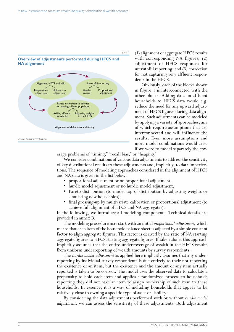
A new instrument to measure wealth inequality: distributional wealth accounts
70 OESTERREICHISCHE NATIONALBANK
(1) alignment of aggregate HFCS results with corresponding NA figures; (2) adjustment of HFCS responses for untruthful reporting; and (3) correction for not capturing very affluent respon-dents in the HFCS.
Obviously, each of the blocks shown in figure 1 is interconnected with the other blocks. Adding data on affluent households to HFCS data would e.g. reduce the need for any upward adjust-ment of HFCS figures during data align-ment. Such adjustments can be modeled by applying a variety of approaches, any of which require assumptions that are interconnected and will influence the results. Even more assumptions and more model combinations would arise if we were to model separately the cov-
erage problems of “timing,” “recall bias,” or “heaping.” We consider combinations of various data adjustments to address the sensitivity
of key distributional results to these adjustments and, implicitly, to data imperfec-tions. The sequence of modeling approaches considered in the alignment of HFCS and NA data is given in the list below:
• proportional adjustment or no proportional adjustment;• hurdle model adjustment or no hurdle model adjustment;• Pareto distribution (to model top of distribution by adjusting weights or
simulating new households);• final grossing-up by multivariate calibration or proportional adjustment (to
achieve full alignment of HFCS and NA aggregates).In the following, we introduce all modeling components. Technical details are provided in annex B.
The modeling procedure may start with an initial proportional adjustment, which means that each item of the household balance sheet is adjusted by a simple constant factor to align aggregate figures. This factor is derived by the ratio of NA starting aggregate figures to HFCS starting aggregate figures. If taken alone, this approach implicitly assumes that the entire undercoverage of wealth in the HFCS results from uniform underreporting of wealth amounts by survey respondents.
The hurdle model adjustment as applied here implicitly assumes that any under-reporting by individual survey respondents is due entirely to their not reporting the existence of an item, but the existence and the amount of any item actually reported is taken to be correct. The model uses the observed data to calculate a propensity to hold each item and applies a randomized process to households reporting they did not have an item to assign ownership of such item to these households. In essence, it is a way of including households that appear to be relatively close to owning a specific type of asset or liability.
By considering the data adjustments performed with or without hurdle model adjustment, we can assess the sensitivity of these adjustments. Both adjustment
Overview of adjustments performed during HFCS and NA alignment
Figure 1
Source: Authors’ compilation.
Alignment HFCS and NA
Proportional adjustment
Multivariate adjustment
Pareto estimation to correct for missing affluent population
Adding affluent households
Adjusting weights in the HFCS
Untruthful reporting
Hurdlemodel
Proportional adjustment
Alignment of definitions and timing

A new instrument to measure wealth inequality: distributional wealth accounts
MONETARY POLICY & THE ECONOMY Q4/21 71
procedures – hurdle model and proportional adjustment – can be considered a means of correcting for underreporting. The first approach tackles underreporting by adjusting reported values and the second by negating reported non-ownership of an asset or liability.
The central element in all these combinations of approaches is the modeling of “missing” rich households by means of a Pareto distribution (see annex B for more details on the related estimation).22 Using Pareto estimates, we can adjust the weights of the richest households in the HFCS to mimic the Pareto distribution (“adjust weights”) or add some particularly rich synthetic households (“add wealthy households”). This part of data adjustment addresses the possibility that the observed set of households is incorrect because some households are missing altogether or some are incorrectly characterized in terms of their ability to be representative of the population.
The final grossing-up adjustment aligns whatever difference remains between the aggregate figures of the HFCS and the NA. Data alignment is generally not achieved before this step is completed, no matter which of the previous steps were actually performed. Two possible approaches at this stage are simple proportional adjustment or multivariate calibration adjustment. The former uses a simple constant adjustment factor (again, based on the ratio of totals derived from micro- and macrodata). The latter is implemented via a generalized linear weight adjustment with bounds on the adjustment factor that minimizes a quadratic loss function subject to reaching aggregate figures for both the top of the distributions (above the Pareto threshold) and the remainder of the household population.
Each step of this modeling procedure depends on specific assumptions. Unfor-tunately, there is very limited theoretical foundation for the choice of these assumptions. The ad hoc approaches considered here are rather pragmatic; they are often applied as technical solutions to statistical problems. In the following section, we provide estimates of key statistics based on a variety of combined assumptions to explore the sensitivity of these statistics.
3 Results3.1 OverallIn table 1, we report the key results on household wealth in Austria generated in the different modeling approaches described above.23 Table 1 shows the mean, median, Gini coefficient and wealth shares for specific groups for the 16 different modeling approaches resulting from the combinations mentioned above.24
22 Kennickell (2019) shows the importance of the right tail of the net wealth distribution for the wealth distribution. Disslbacher et al. (2020) suggest a unified regression approach to estimate all parameters of a Pareto distribution jointly and extend our analysis by a more flexible three-parameter generalized Pareto estimation. They introduce a new database of national rich lists (ERLDB) as an alternative to commonly used global rich lists to combine with HFCS 2017 data. Furthermore, Kennickell (2021) proposes a new method to estimate a Pareto adjustment without relying on external information for the far end of the wealth distribution, relying only on a reliable estimate for the aggregate level of net wealth.
23 We start with an arbitrary choice of a threshold of EUR 1 million above which the Pareto distribution is used to adjust the affluent part of the distribution. Below, we vary this parameter to explore the impact of our choice of threshold.
24 We use these statistics because experience with almost a decade of HFCS results has shown that these statistics are most widely discussed.

A new instrument to measure wealth inequality: distributional wealth accounts
72 OESTERREICHISCHE NATIONALBANK
Across all sets of adjustments, the mean of net wealth increases from EUR 237,000 in the unadjusted data to about EUR 332,000. This result and its stability are attributable to the last step of the whole modeling procedure where aggregate figures are fixed to the NA and the population is given exogenously. This deter-mines the mean of net wealth. The median net wealth, however, varies strongly across adjustments. In the most extreme case, it almost doubles. The changes relative to the baseline (HFCS result) show an increase of about 75%. The Gini coefficients differ by about 0.1 (i.e. about 15%), depending on the choice of adjust-ments. Looking at the shares in net wealth, results for the bottom shares are more stable, in absolute terms, than results for the top shares. This points even more strongly toward the need to carefully model the top of the net wealth distribution. While the bottom 50% of the household population hold about 2.5% of total net wealth (HFCS results), simulated wealth levels yield a negative share of the bottom 50% in some cases of the multivariate calibration, which results from high levels of household debt.
In general, as the last step of the adjustment procedure, multivariate calibration produces higher levels of inequality. The mechanism behind this calibration method tries to achieve an alignment of aggregate NA and HFCS figures while changing household weights as little as possible. This implies increasing the weights of wealthy households to raise aggregate wealth levels in the HFCS. Thus, the mechanics of multivariate calibration in comparison with proportional adjustment –
Table 1
Net wealth simulations performed to align HFCS and NA aggregates – overview
Mean Median Gini coeffi-cent
Share in net wealth
Top 1% Top 10% Bottom 50%
EUR thousand %
Unadjusted HFCS results 236.5 70.9 0.748 23.7 57.9 2.5Adjustment modelsPrior proportional adjustment
Hurdle model
Pareto adjust weights, multivariate calibration 331.9 121.1 0.788 26.2 63.5 2.1Pareto adjust weights, proportional adjustment 331.9 123.3 0.771 25.7 59.9 2.3Pareto add wealthy households, multivariate calibration 331.6 113.7 0.814 32.6 66.4 1.3Pareto add wealthy households, proportional adjustment 331.6 115.3 0.791 32.6 62.3 1.8
No prior proportional adjustment
Pareto adjust weights, multivariate calibration 331.9 81.0 0.849 34.3 70.3 –0.5Pareto adjust weights, proportional adjustment 331.9 109.3 0.789 26.6 61.2 1.2Pareto add wealthy households, multivariate calibration 331.6 76.8 0.828 44.6 70.4 1.4Pareto add wealthy households, proportional adjustment 331.6 90.8 0.785 37.8 64.8 2.5
Prior proportional adjustment
No hurdle model
Pareto adjust weights, multivariate calibration 331.8 99.5 0.821 27.7 65.7 0.2Pareto adjust weights, proportional adjustment 331.8 102.7 0.804 27.5 62.6 0.5Pareto add wealthy households, multivariate calibration 331.6 90.5 0.841 33.6 68.2 –0.4Pareto add wealthy households, proportional adjustment 331.6 93.3 0.821 33.9 64.7 0.1
No prior proportional adjustment
Pareto adjust weights, multivariate calibration 332.0 73.2 0.873 37.9 72.1 –1.4Pareto adjust weights, proportional adjustment 332.0 105.7 0.799 27.8 61.7 0.6Pareto add wealthy households, multivariate calibration 331.6 71.0 0.837 47.5 71.3 1.0Pareto add wealthy households, proportional adjustment 331.6 86.3 0.787 38.2 64.9 2.5
Minimum 331.6 71.0 0.771 25.7 59.9 –1.4Maximum 332.0 123.3 0.873 47.5 72.1 2.5
Source: HFCS Austria 2017, OeNB; trend rich list 2017; national accounts (OeNB, Statistics Austria).
Note: In absolute values, the net wealth of the top 10% (1%) of the distribution according to unadjusted HFCS results ranges from EUR 525,000 (EUR 2.1 million) to close to EUR 70 million. After the adjustment process, these figures are naturally higher.

A new instrument to measure wealth inequality: distributional wealth accounts
MONETARY POLICY & THE ECONOMY Q4/21 73
i.e. multiplying the wealth of each household by a constant factor – are associated with higher levels of inequality.25 Furthermore, the approach of simulating new households (“add wealthy households”) yields more top-sensitive results, i.e. a higher level of estimated inequality (measured as top shares), given the scenario definition. We must keep in mind that the newly simulated households by defini-tion own extremely high levels of net wealth and hence belong to the most affluent part of the population. Applying hurdle model and proportional adjustment before modeling the affluent population results in a less systematic impact.
Overall, the mean and the share of the bottom 50% of the population seem to be (much) more stable than the inequality indicator, median levels and top shares. This indicates how important it is to model the affluent part of the population. In the next two subsections, we take an in-depth look at measuring the top of the distribution. According to our estimations, the wealth ownership share of the top 1% of the distribution ranges between one-quarter and one-half.
3.2 Modeling the right tail of the net wealth distribution
In a next step, we look at the illustrative example of a set of adjustments that consist of an estimation of a Pareto distribution to simulate the top of the wealth distribution (by employing both versions, i.e. “adjust weights” and “add affluent households”) followed by a multivariate calibration to align HFCS and NA data. Vermeulen (2018) e.g. shows that the affluent part of the wealth distribution plays an important role. Piketty et al. (2021) provide a historical contextualization of the top of the wealth distribution. With our example, we take the analysis one step further by concentrating only on important assumptions when it comes to modeling the top of the wealth distribution. In choosing this approach, we implicitly assume truthful reporting in the HFCS (i.e. we neither perform a proportional adjustment nor a hurdle model adjustment).
Table 2 shows key statistics, i.e the mean, median and inequality measures and shares for specific groups of net wealth. We show the results for unadjusted HFCS 2017 data and 12 different variants of modeling the top of the wealth distribution. Table 2 also shows the minimum and maximum values resulting from the different modeling variants to allow for direct comparison.
25 We should like to thank our referee for pointing out this line of thought.
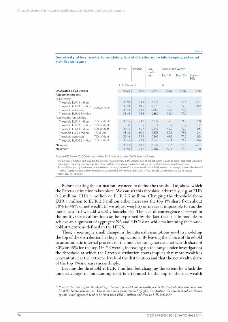
A new instrument to measure wealth inequality: distributional wealth accounts
74 OESTERREICHISCHE NATIONALBANK
Before starting the estimation, we need to define the threshold w0 above which the Pareto estimation takes place. We can set this threshold arbitrarily, e.g. at EUR 0.5 million, EUR 1 million or EUR 2.5 million. Changing the threshold from EUR 1 million to EUR 2.5 million either increases the top 1% share from about 38% to 48% of net wealth (if we adjust weights) or makes it impossible to run the model at all (if we add wealthy households). The lack of convergence observed in the multivariate calibration can be explained by the fact that it is impossible to achieve an alignment of aggregate NA and HFCS data while maintaining the house-hold structure as defined in the HFCS.
Thus, a seemingly small change in the internal assumptions used in modeling the top of the distribution has huge implications. By leaving the choice of threshold to an automatic internal procedure, the modeler can generate a net wealth share of 30% or 45% for the top 1%.26 Overall, increasing (in the range under investigation) the threshold at which the Pareto distribution starts implies that more wealth is concentrated at the extreme levels of the distribution and that the net wealth share of the top 1% increases accordingly.
Leaving the threshold at EUR 1 million but changing the extent by which the undercoverage of outstanding debt is attributed to the top of the net wealth
26 If we set the choice of the threshold w0 to “auto,” the model automatically selects the threshold that maximizes the fit of the Pareto distribution. This is done via a mean residual life plot. For Austria, the threshold values selected by this “auto” approach tend to be lower than EUR 1 million and close to EUR 500,000.
Table 2
Sensitivity of key results to modeling top of distribution while keeping external rich list constant
Mean Median Gini coeffi-cient
Share in net wealth
Top 1% Top 10% Bottom 50%
EUR thousand %
Unadjusted HFCS results 236.5 70.9 0.748 23.67 57.87 2.48Adjustment modelsAdjust weight
Threshold EUR 1 million
xx% of debt1
332.0 73.2 0.873 37.9 72.1 –1.4Threshold EUR 2.5 million 331.8 69.5 0.873 48.0 72.8 –0.9Threshold automatic 331.2 74.2 0.858 30.6 70.3 –1.1Threshold EUR 0.5 million 331.4 73.9 0.860 31.4 70.7 –1.1
Add wealthy householdsThreshold EUR 1 million 75% of debt2 331.6 71.0 0.837 47.5 71.3 1.0Threshold EUR 2.5 million 75% of debt x3 x x x x xThreshold EUR 1 million 30% of debt 331.6 66.7 0.849 48.0 72.1 0.5Threshold EUR 1 million 1% of debt 331.6 60.0 0.909 50.7 75.5 –2.4Threshold automatic 75% of debt 331.6 71.9 0.845 44.7 71.5 0.5Threshold EUR 0.5 million 75% of debt 331.6 72.2 0.845 45.1 71.7 0.6
Minimum 331.2 60.0 0.837 30.6 70.3 –2.4Maximum 332.0 74.2 0.909 50.7 75.5 1.0
Source: HFCS Austria 2017, OeNB; trend rich list 2017; national accounts (OeNB, Statistics Austria).1 The portfolio allocation, and thus also the extent of debt holdings, of the aff luent part of the population is given by survey responses. Additional
assumptions regarding debt holdings (and other portfolio choices) only need to be made for the “add wealthy households” approach.2 As the aff luent part of the distribution is modeled in terms of net wealth (i.e. gross wealth minus debt), we need an assumption about the share of
“missing’’ aggregate debt held by the simulated households (“add wealthy households”). Thus, we vary this parameter to see its impact.3 Model does not converge.

A new instrument to measure wealth inequality: distributional wealth accounts
MONETARY POLICY & THE ECONOMY Q4/21 75
distribution – considering three different ad hoc levels of 75%, 30% and 1% – only has an effect in the method “add wealthy households” because in the “adjust weights” method, the portfolio allocation is given by the households in the HFCS. The Gini coefficient e.g. changes from 0.84 to 0.91 and is getting close to maximum inequality. Also the median level of net wealth could substantially decrease under these conditions. In general, the more debt is held by the top, the lower the inequality measured by the Gini coefficient and the top 1% share.
3.3 Information on the right tail of the net wealth distribution
So-called rich lists are important data sources in modeling the top of the net wealth distribution. However, these lists exhibit serious problems of data quality and lack transparency (see section 2). In the following estimation procedure, we use various sources of information to analyze their respective impact on the results. This approach may shed light on what happens if one country uses one type of informa-tion while other countries opt for a different type – choices that may e.g. depend on data availability per country. We use information from a rich list for Austria provided by an Austrian business magazine (trend list), data on wealthy Austrians included in the Forbes rich list, some corresponding OeNB in-house information as well as information obtained from the Sabina business register. We use the latter because wealth and business wealth are highly correlated.27
Table 3 follows the same structure as table 2. For this exercise, we leave all the other modeling assumptions constant, meaning that again we start from the approach of employing no initial proportional adjustment and no hurdle model adjustment.
27 See e.g. the new sampling strategy employed in the German Socio-Economic Panel (SOEP), (Schröder et al., 2020).
Table 3
Sensitivity of key results to modeling the top of the distribution by employing various rich lists
Mean Median Gini coeffi-cient
Share in net wealth
Top 1% Top 10% Bottom 50%
EUR thousand %
Unadjusted HFCS results 236.5 70.9 0.748 23.67 57.87 2.48Adjustment modelsAdjust weight, threshold EUR 1 million
trend rich list 332.0 73.2 0.873 37.9 72.1 –1.4Forbes rich list 331.9 79.1 0.849 32.3 67.9 –1.2OeNB in-house information 332.0 74.5 0.867 36.4 70.9 –1.4Business equity holdings 331.8 80.7 0.842 30.6 66.6 –1.1
Add wealthy households, threshold EUR 1 million, 75% of debttrend rich list 331.6 71.0 0.837 47.5 71.3 1.0Forbes rich list 331.7 81.8 0.788 35.6 65.0 2.2OeNB in-house information 331.6 72.9 0.824 44.7 69.8 1.4Business equity holdings 331.7 83.5 0.784 32.2 64.0 2.1
Minimum 332 71 0.784 30.6 64.0 –1.4Maximum 332 84 0.873 47.5 72.1 2.2
Source: HFCS Austria 2017, OeNB; various rich lists for 2017; national accounts (OeNB, Statistics Austria).

A new instrument to measure wealth inequality: distributional wealth accounts
76 OESTERREICHISCHE NATIONALBANK
Especially for the net wealth shares of the top of the distribution and for the Gini coefficient we find that the specific choice of a rich list has a strong impact. The Gini coefficient varies within a range of close to 10 points, depending on the choice of list. Furthermore, the net wealth share of the top 1% varies between about 30% and almost 50%. The median of wealth varies sizably across different rich lists.
Which information yields what type of results is difficult to discern. For the Gini coefficient and the net wealth shares of the top 1% and top 10%, there seems to be a consistent pattern, with the approach using the business register database (Sabina) list resulting in the lowest values and that using the Forbes list in the second lowest, while the results of the approaches employing OeNB in-house information and the trend list are reasonably close. One might have expected the Sabina-based values to be lowest since Sabina data exclude wealth other than business wealth. Still, the overall impact of the choice of external information on the top of the distribution cannot be denied. Thus, we use these results to argue for a cautious approach to cross-country comparisons that use different data sources in Pareto adjustments to estimated wealth distributions (Fessler and Schürz, 2013).
3.4 Modeling the top and its impact on the distribution
The sensitivity of the overall distribution of net wealth to changes made to the top of the distribution can be analyzed by decomposing the overall distribution into subgroups defined by their position within the distribution. Cowell at al. (2017) showed that the Gini coefficient can be decomposed as follows:
= ℎ + ℎ +
where GC is the Gini coefficient, shg denotes the share of net wealth held by group
∈ ( [95%]; [5%])
and pg is the population share of group g. The remaining term (BI) is the be-tween-inequality of both groups; this is the GC if each member of the two groups has the group-specific mean net wealth level.
Table 4 displays the results of this exercise. We show a group breakdown by percentiles (top 5% vs. remainder) as well as a breakdown by threshold used in the Pareto estimation. It is of particu-lar importance that the largest contribu-tion to inequality stems from be-tween-inequality.
The choice of how to model the affluent population – that is the decision to use a rich list or not – has a huge im-pact on the GC of the subpopulations
Table 4
Decomposing the Gini coefficient of net wealth
trend rich list No specific adjustment of top of distribution1
Top 5% Pareto threshold EUR 1 million
Top 5% EUR 1 million
Gini coefficient 0.837 0.837 0.837 0.837Population share: affluent households in % 5 4 5 7Within inequality: affluent households 0.698 0.700 0.475 0.470Population share: other households in % 95 96 95 93Within inequality: other households 0.678 0.682 0.781 0.787Between-inequality 0.573 0.553 0.465 0.513
Contribution to inequality %
Total (1+2+3) 100 100 100 100of which: aff luent population (1) 3 2 1 2
rest of population (2) 29 32 43 36between-inequality (3) 68 66 56 61
Source: HFCS Austria 2017, OeNB; trend rich list 2017; national accounts (OeNB, Statistics Austria).1 In the two columns below, we do not model the aff luent part of the net wealth distribution with the Pareto
distribution, but instead achieve alignment with NA data only through multivariate adjustment.

A new instrument to measure wealth inequality: distributional wealth accounts
MONETARY POLICY & THE ECONOMY Q4/21 77
and on the resulting between-inequality. This holds despite an almost exact equality of the overall GC.
4 ConclusionsThis study focuses on important caveats in aligning micro- and macrodata on household wealth in Austria. A thorough analysis of households’ assets and liabilities requires detailed microdata and improved macrodata, i.e. national accounts (NA) data. Peoples’ reported perceptions of the value of their assets, overall, do not align well with corresponding aggregate market values recorded in the NA.
We use various standard modeling approaches to align data stemming from two data sources, namely the Household Finance and Consumption Survey (HFCS) and the NA. Our results on top wealth shares in Austria are highly sensitive to the modeling assumptions. Given huge discrepancies in the obtained results, we find the information content of wealth inequality data to be rather limited. Given the present data limitations, it is difficult to calculate policy models, e.g. for wealth taxes or inheritance taxes. Overall, we therefore argue that the information contained in the newly developed distributional wealth accounts should be analyzed with caution. Based on the results of our modeling exercise for Austria, our conjecture is that international comparisons – but also the development of national wealth inequality indicators over time – might be flawed by differences in modeling assumptions or the availability of underlying data that are used in the background.
ReferencesAndreasch, M. and P. Lindner. 2016. Micro- and Macrodata: a Comparison of the Household
Finance and Consumption Survey with Financial Accounts in Austria. In: Journal of Official Statistics. Volume 32. No. 1. 1–28.
Albacete, N. 2014. Multiple Imputations in the Household Survey on Housing Wealth. In: Austrian Journal of Statistics 43(1). 5–28. https://doi.org/10.17713/ajs.v43i1.4
Albacete, N., S. Dippenaar, P. Lindner and K. Wagner. 2018. Eurosystem Household Finance and Consumption Survey 2017: Methodological notes for Austria. Monetary Policy & the Economy Q4/18 – Addendum. OeNB.
Biancotti, C., G. D’Alessio and A. Neri. 2008. Measurement error in the Bank of Italy’s survey of household income and wealth. In: Review of Income and Wealth 54. 466–493. https://doi.org/10.1111/j.1475-4991.2008.00283.x
Chancel, L. 2021. World Inequality Report 2020.Cowell, F., B. Nolan, J. Olivera and P. Van Kerm. 2017. Wealth, Top Incomes and Inequality.
LWS Working papers 24. LIS Cross-National Data Center in Luxembourg.Disslbacher, F. M., E. Ertl, P. List, M. Mokre and M. Schnetzer 2020. On Top of the Top
- Adjusting wealth distributions using national rich list. INEQ-WP 20.Doepke, M., M. Schneider and V. Selezneva 2019. Distributional effects of monetary policy
Paper presented at the Money Macro Workshop of the ECB 2019. https://www.ecb.europa.eu/pub/conferences/shared/pdf/20190321_money_macro_workshop/Doepke_Distributional_Ef-fects_of_Monetar_%20Policy.pdf
ECB 2020a. The Household Finance and Consumption Survey: Methodological report for the 2017 wave. Statistics Paper Series 35.
ECB 2020b. Understanding household wealth: linking macro and micro data to produce distribu-tional financial accounts. Statistics Paper Series 37.

A new instrument to measure wealth inequality: distributional wealth accounts
78 OESTERREICHISCHE NATIONALBANK
European Statistical System. 2019. Quality Assurance Framework of the European Statistical System. Version 2.0 available from https://ec.europa.eu/eurostat/documents/64157/4392716/ESS-QAF-V2.0-final.pdf
Fessler, P. and M. Schürz 2013. Cross-country comparability of the Eurosystem Household Finance and Consumption Survey. In: Monetary Policy & Economy Q2/13. OeNB. 29–50.
Fessler, P., P. Lindner and M. Schürz. 2018. Eurosystem Household Finance and Consumption Survey 2017: First Results for Austria. In: Monetary Policy & the Economy Q4/18. OeNB. 36–66.
Gabaix, X. and R. Ibragimov. 2011. Rank 21=2: A Simple Way to Improve the OLS Estimation of Tail Exponents. In: Journal of Business and Economic Statistics 29. 24–39.
GEWINN-Magazin. 2019. Wald Millionäre. 7/819. 22–30.Humer, S., M. Moser, M. Ertl and M. Schnetzer. 2021. The Micro-Macro Gap in Property
Incomes: Consequences for Household Income Inequality. Mimeo.Kennickell, A. B. 2017a. Try, try again: response and nonresponse in the 2009 SCF Panel Statistical
Journal of the IAOS Volume 33/1. 203–209.Kennickell, A. B. 2017b. Look again. Editing and imputation of SCF panel data. In: Statistical
Journal of the IAOS 33/1. 195–202. DOI: 10.3233/SJI-160268.Kennickell, A. B. 2019. The tail that wags: differences in effective right tail coverage and estimates
of wealth inequality. In: The Journal of Economic Inequality 17/5. 443–459. https://doi.org/10.1007/s10888-019-09424-8.
Kennickell, A. B. 2021. Chasing the Tail: A Generalized Pareto Distribution Approach to Estimating Wealth Inequality. SocArXiv u3zs2. Center for Open Science.
Le Roux, J. and M. Roma. 2019 Accuracy and determinants of self-assessed euro area house prices. ECB Working Paper Series 2328. November.
Lustig, N. 2015. The missing rich in household surveys: a survey of causes and correction methods. CEO Institute.
Mooslechner, P., H. Schuberth and M. Schürz (eds.). 2004. Economic Policy under Uncer-tainty – the role of truth and accountability in policy advice. Edward Elgar.
Neri, A. and M. Giovanna Ranalli. 2012 To misreport or not to report? The measurement of household financial wealth. Banca d’Italia Working Paper Number 870.
Piketty, T., E. Saez and G. Zucman. 2021. Twenty Years and Counting: Thoughts about Measuring the Upper Tail. Prepared for the Journal of Economic Inequality (special issue on the upper tail) downloadable from https://gabriel-zucman.eu/files/PSZ2021JOEI.pdf
Schröder, C., C. Bartels, K. Göbler, M. M. Grabka, J. König, R. Siegers and S. Zinn. 2020. Improving the Coverage of the Top-Wealth Population in the Socio-Economic Panel (SOEP). SOEP papers on Multidisciplinary Panel Data Research at DIW Berlin. SOEP papers 1114.
Stiglitz, J., A. Sen and J. Fitoussi. 2009. Report of the Commission on the Measurement of Economic Performance and Social Progress (CMEPSP).
Vermeulen, P. 2018. How Fat is the Top Tail of the Wealth Distribution? In: Review of Income and Wealth, International Association for Research in Income and Wealth 64/2. 357–387. June.

A new instrument to measure wealth inequality: distributional wealth accounts
MONETARY POLICY & THE ECONOMY Q4/21 79
Annex AAdditional tablesTable A1 as in Albacete et al. (2018); table A2 as in the ECB’s methodological documentation for the HFCS (ECB, 2020a).
Table A1
Item nonresponse for selected variables (unweighted)
Household has item
Responses by households that have the item
Yes Un- known
Amount Range “Don’t know”/ “No answer”
Other missing values1
(1) (2) (3) (4) (5) (6)
%
Value of main residence2 37.4 0.0 82.0 14.9 2.8 0.3HMR mortgage 1: amount still owed 12.5 0.2 81.8 8.6 8.6 1.0Monthly amount paid as rent 56.6 0.0 59.7 39.8 0.5 0.0Other property 1: current value 12.7 0.1 77.9 16.2 4.9 1.0Other property mortgage 1: amount still owed 1.4 0.1 79.1 2.3 14.0 4.7Value of sight accounts 99.4 0.0 83.8 8.0 8.1 0.1Value of saving accounts 98.7 1.3 81.0 9.0 5.3 4.7Value of publicly traded shares 4.7 0.5 82.5 11.9 5.6 0.0Amount owed to household 6.6 0.2 94.6 3.4 2.0 0.0Employment status (main activity) (person 1) 100.0 0.0 100.0 0.0 0.0 0.0Gross employee income (person 1) 53.3 0.0 91.3 6.6 1.9 0.2Gross income from unemployment benefits (person 1) 6.6 0.0 87.2 9.9 3.0 0.0Gross income from financial investments 63.8 11.7 54.8 34.5 9.3 1.4Gift/inheritance 1: value 27.2 1.2 84.6 7.3 5.4 2.8Amount spent on food at home 100.0 0.0 95.9 4.0 0.1 0.0
Source: HFCS Austria 2017, OeNB.
Note: HMR = household main residence.1 Missing values due to editing measures and exits from loops.2 Based on the HB0900 variable.
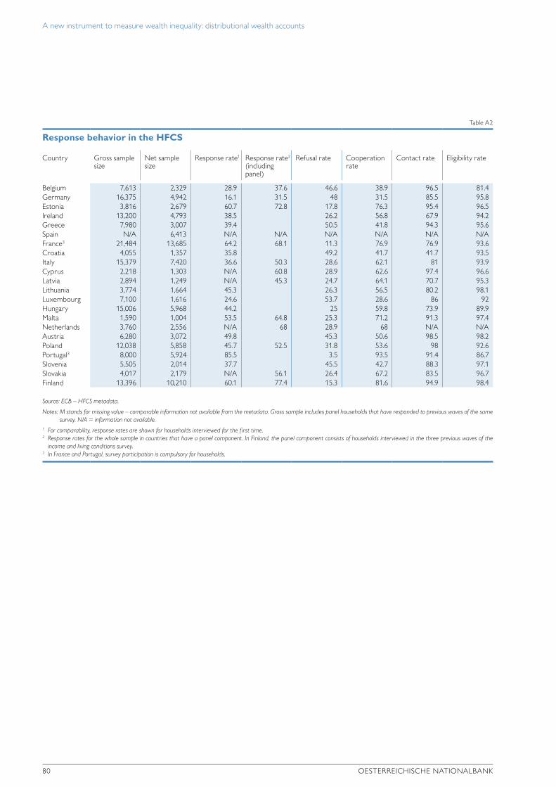
A new instrument to measure wealth inequality: distributional wealth accounts
80 OESTERREICHISCHE NATIONALBANK
Annex BTechnical introduction to the modeling approaches applied in this studyAs described in the main text, households’ net wealth contains various assets and liabilities. Adjustments can be made for a specific asset or liability or for net wealth itself, depending on the data sources available. If adjustments are made for net wealth itself and if we wish to obtain results on asset classes at the same time, we need to split the change across asset classes afterward. Proportional adjustment and hurdle model adjustment are often performed on a specific item while Pareto adjustment is implemented for the net wealth of households.
Proportional adjustment
The simplest approach to align aggregate figures A from the HFCS and the NA is to calculate the factor mc for each asset and liability component c by dividing aggregate values, i.e.
= .
.
Multiplying each individuals’ holding of each asset and liability by mc ensures align-ment of the two data sources. This approach assumes, however, that all responses in the HFCS are wrong and are off by relatively the same amount, which is very unlikely to be the case.
Another difficulty arises from the (implicit) assumption at which step in the modeling procedure which proportional adjustment is performed. In our study, we illustrate cases where we perform proportional adjustment at the beginning and at the end of the procedure, respectively. We will show below that proportional adjustment is an alternative to multivariate calibration when it comes to aligning aggregate figures.
Hurdle model
In the HFCS, responding households are asked, for each item of their balance sheet, whether they hold this specific item (yes/no). If they answer “yes,” they are asked to specify the corresponding amount. In the type of adjustment considered here, the “no” response is assumed to be incorrect for part of the group reporting not to hold a specific asset. Information on the share of wrongly collected “no” answers is rarely available. However, we can estimate a logit model to simulate the likelihood of respondents holding a specific balance sheet item C, given the observed data and letting C be the choice variable of holding an item and C the value of this item. The logit model can be written as
( = 1| , … , ) = ( , … , )
where ( , … , ) ∈ are several explanatory factors. The function f() is the logistic distribution function so that the model can be written as
( = 1| , … , ) = ( ⋯ ) ( ⋯ )
.
Table A2
Response behavior in the HFCS
Country Gross sample size
Net sample size
Response rate1 Response rate2 (including panel)
Refusal rate Cooperation rate
Contact rate Eligibility rate
Belgium 7,613 2,329 28.9 37.6 46.6 38.9 96.5 81.4Germany 16,375 4,942 16.1 31.5 48 31.5 85.5 95.8Estonia 3,816 2,679 60.7 72.8 17.8 76.3 95.4 96.5Ireland 13,200 4,793 38.5 26.2 56.8 67.9 94.2Greece 7,980 3,007 39.4 50.5 41.8 94.3 95.6Spain N/A 6,413 N/A N/A N/A N/A N/A N/AFrance3 21,484 13,685 64.2 68.1 11.3 76.9 76.9 93.6Croatia 4,055 1,357 35.8 49.2 41.7 41.7 93.5Italy 15,379 7,420 36.6 50.3 28.6 62.1 81 93.9Cyprus 2,218 1,303 N/A 60.8 28.9 62.6 97.4 96.6Latvia 2,894 1,249 N/A 45.3 24.7 64.1 70.7 95.3Lithuania 3,774 1,664 45.3 26.3 56.5 80.2 98.1Luxembourg 7,100 1,616 24.6 53.7 28.6 86 92Hungary 15,006 5,968 44.2 25 59.8 73.9 89.9Malta 1,590 1,004 53.5 64.8 25.3 71.2 91.3 97.4Netherlands 3,760 2,556 N/A 68 28.9 68 N/A N/AAustria 6,280 3,072 49.8 45.3 50.6 98.5 98.2Poland 12,038 5,858 45.7 52.5 31.8 53.6 98 92.6Portugal3 8,000 5,924 85.5 3.5 93.5 91.4 86.7Slovenia 5,505 2,014 37.7 45.5 42.7 88.3 97.1Slovakia 4,017 2,179 N/A 56.1 26.4 67.2 83.5 96.7Finland 13,396 10,210 60.1 77.4 15.3 81.6 94.9 98.4
Source: ECB – HFCS metadata.
Notes: M stands for missing value – comparable information not available from the metadata. Gross sample includes panel households that have responded to previous waves of the same survey. N/A = information not available.
1 For comparability, response rates are shown for households interviewed for the first time.2 Response rates for the whole sample in countries that have a panel component. In Finland, the panel component consists of households interviewed in the three previous waves of the
income and living conditions survey.3 In France and Portugal, survey participation is compulsory for households.

A new instrument to measure wealth inequality: distributional wealth accounts
MONETARY POLICY & THE ECONOMY Q4/21 81
Annex BTechnical introduction to the modeling approaches applied in this studyAs described in the main text, households’ net wealth contains various assets and liabilities. Adjustments can be made for a specific asset or liability or for net wealth itself, depending on the data sources available. If adjustments are made for net wealth itself and if we wish to obtain results on asset classes at the same time, we need to split the change across asset classes afterward. Proportional adjustment and hurdle model adjustment are often performed on a specific item while Pareto adjustment is implemented for the net wealth of households.
Proportional adjustment
The simplest approach to align aggregate figures A from the HFCS and the NA is to calculate the factor mc for each asset and liability component c by dividing aggregate values, i.e.
= .
.
Multiplying each individuals’ holding of each asset and liability by mc ensures align-ment of the two data sources. This approach assumes, however, that all responses in the HFCS are wrong and are off by relatively the same amount, which is very unlikely to be the case.
Another difficulty arises from the (implicit) assumption at which step in the modeling procedure which proportional adjustment is performed. In our study, we illustrate cases where we perform proportional adjustment at the beginning and at the end of the procedure, respectively. We will show below that proportional adjustment is an alternative to multivariate calibration when it comes to aligning aggregate figures.
Hurdle model
In the HFCS, responding households are asked, for each item of their balance sheet, whether they hold this specific item (yes/no). If they answer “yes,” they are asked to specify the corresponding amount. In the type of adjustment considered here, the “no” response is assumed to be incorrect for part of the group reporting not to hold a specific asset. Information on the share of wrongly collected “no” answers is rarely available. However, we can estimate a logit model to simulate the likelihood of respondents holding a specific balance sheet item C, given the observed data and letting C be the choice variable of holding an item and C the value of this item. The logit model can be written as
( = 1| , … , ) = ( , … , )
where ( , … , ) ∈ are several explanatory factors. The function f() is the logistic distribution function so that the model can be written as
( = 1| , … , ) = ( ⋯ ) ( ⋯ )
.
Table A2
Response behavior in the HFCS
Country Gross sample size
Net sample size
Response rate1 Response rate2 (including panel)
Refusal rate Cooperation rate
Contact rate Eligibility rate
Belgium 7,613 2,329 28.9 37.6 46.6 38.9 96.5 81.4Germany 16,375 4,942 16.1 31.5 48 31.5 85.5 95.8Estonia 3,816 2,679 60.7 72.8 17.8 76.3 95.4 96.5Ireland 13,200 4,793 38.5 26.2 56.8 67.9 94.2Greece 7,980 3,007 39.4 50.5 41.8 94.3 95.6Spain N/A 6,413 N/A N/A N/A N/A N/A N/AFrance3 21,484 13,685 64.2 68.1 11.3 76.9 76.9 93.6Croatia 4,055 1,357 35.8 49.2 41.7 41.7 93.5Italy 15,379 7,420 36.6 50.3 28.6 62.1 81 93.9Cyprus 2,218 1,303 N/A 60.8 28.9 62.6 97.4 96.6Latvia 2,894 1,249 N/A 45.3 24.7 64.1 70.7 95.3Lithuania 3,774 1,664 45.3 26.3 56.5 80.2 98.1Luxembourg 7,100 1,616 24.6 53.7 28.6 86 92Hungary 15,006 5,968 44.2 25 59.8 73.9 89.9Malta 1,590 1,004 53.5 64.8 25.3 71.2 91.3 97.4Netherlands 3,760 2,556 N/A 68 28.9 68 N/A N/AAustria 6,280 3,072 49.8 45.3 50.6 98.5 98.2Poland 12,038 5,858 45.7 52.5 31.8 53.6 98 92.6Portugal3 8,000 5,924 85.5 3.5 93.5 91.4 86.7Slovenia 5,505 2,014 37.7 45.5 42.7 88.3 97.1Slovakia 4,017 2,179 N/A 56.1 26.4 67.2 83.5 96.7Finland 13,396 10,210 60.1 77.4 15.3 81.6 94.9 98.4
Source: ECB – HFCS metadata.
Notes: M stands for missing value – comparable information not available from the metadata. Gross sample includes panel households that have responded to previous waves of the same survey. N/A = information not available.
1 For comparability, response rates are shown for households interviewed for the first time.2 Response rates for the whole sample in countries that have a panel component. In Finland, the panel component consists of households interviewed in the three previous waves of the
income and living conditions survey.3 In France and Portugal, survey participation is compulsory for households.

A new instrument to measure wealth inequality: distributional wealth accounts
82 OESTERREICHISCHE NATIONALBANK
This model can be estimated with a generalized linear method.28 It is used to predict the likelihood of holding a particular item of a household’s balance sheet. Taking a random draw from the uniform distribution within the interval of zero and one, one can determine whether a negative answer can be assumed to be false. If the prediction obtained from the logit model is higher than the random draw, a particular household is simulated to hold the particular item (i.e. we set the “no” answer [false negative] to “yes”).
Once it has been decided which “no” answer was falsely recorded and thus had to be changed to “yes,” we need to impute the actual value of the respective item that is held by a household. For this step, an OLS regression is estimated in the following form
= + + ⋯+ + .
.
Derived coefficients are used to impute the missing values. In principle, there is no theoretical reason why the logit model and the OLS
regression should have an identical or a similar set of explanatory variables X. Albacete (2014) and Kennickell (2017a and 2017b) provide a more in-depth discus-sion of explanatory variables that should be used in such an imputation procedure. To keep it simple, as the best selection of explanatory variables X is not the focus of our paper, we use the same set of explanatory variables. It contains income, the number of household members, employment status, position of the household in the wealth distribution as originally determined in the HFCS (wealth decile) and level of education. Only the information on income is used as a continuous variable. All the other variables are categorical or dummies.
All balance sheet items can be adjusted by employing this procedure. The impact of adjustments on results varies. Balance sheet items such as deposits, which almost every household owns, are affected only slightly by employing this procedure, whereas other items that are held be fewer households might be affected more heavily.
Pareto adjustment
As discussed in the main text, wealth surveys typically have difficulties in reaching the top end of the wealth distribution. For this reason, the literature suggests using a Pareto distribution in the adjustment procedure. This suggestion is based on the generally accepted assumption that the top of the net wealth distribution follows a power law. Denote net wealth by w. The pdf [ f(w)] and cdf [F(w)] of the Pareto distribution are defined by
( ) = ≥
0 <
( ) =1 − ( ) ≥
0 <
28 In R, the package “svyglm“ is used to take weighting into account.

A new instrument to measure wealth inequality: distributional wealth accounts
MONETARY POLICY & THE ECONOMY Q4/21 83
Thus, the distribution is defined by two parameters: wo, a threshold above which the distribution is assumed to apply, and α, a “shape” parameter. We vary wo in our exercise to see the effect of the choice of this assumption on the results. α is esti-mated via an OLS regression based on the complementary cumulative distribution function, incorporating a bias correction (Vermeulen, 2018; Gabaix and Ibragimov, 2011) for the survey results. As discussed in the main text, to estimate the Pareto distribution, we supplement the observed HFCS data with data from several so-called rich lists. These added observations are included with a weight of one.
Once the specific form of the Pareto distribution is estimated, we need to either adjust the weights of households in such a way that the right tail follows this distribution or impute new households that follow this distribution.29 In the first approach, “adjust weight,” the Pareto’s α is estimated for the data from the HFCS as well as for observations from the rich lists (denoted â) and separately for the HFCS alone (denoted α’). Denoting the weight of a household i by
i, we can
adjust the weights of households above wo by the factor
= ( | , )( | , )
,
,
so that the top follows the estimated Pareto distribution including the information obtained from the rich lists. This procedure does not impact the net wealth levels held by individual households but only the household weight attached to it. This implies, however, that this modeling approach does not only change balance sheet information but also all other information, e.g. the estimates on sociodemographic characteristics. To avoid this second effect, we use a calibration method based on a quadradic loss function30 to retain the original distribution of sociodemographic information (age, education, gender, labor status, household size and total house-hold population). To achieve both the top of the distribution that follows the Pareto distribution and maintain the original sociodemographic information, an iterative procedure of the Pareto estimation and calibration is implemented until α’ (incor-porating the previous iteration’s adjustments) and â converge.
Instead of adjusting household weights, we can also simulate synthetic house-holds from the estimated Pareto distribution. To do so, we subdivide the potential wealth range above wo into three parts: the part above wo and below (and including) the maximum value observed in the HFCS (wα
maxHFCS), the range between the maximum HFCS value and below the lowest observation in the rich list (wα
minRich), and the part above wα
minRich. We only simulate households in the middle range. Given the number of households in the first part (denoted SHFCS) and the i.i.d. assumption, the number of households Stop to be simulated is
= 0 ℎ− 0
ℎ − 0 ℎ.
.
Given the number of synthetic households to be simulated, their net wealth levels can be drawn from the Pareto distribution with the estimated α and the assumed wo. These households enter the data with a weight of one. Note, however, that the
29 We could also implement a hybrid approach by adjusting weights and imputing new households. In this paper, we refrain from this possibility, however.
30 Similar to the multivariate calibration method described in more detail below.

A new instrument to measure wealth inequality: distributional wealth accounts
84 OESTERREICHISCHE NATIONALBANK
portfolio allocation of these households and their sociodemographic characteristics are not known. In particular, an additional assumption must be made concerning liability holdings and thus implicitly determining the coverage rates of the HFCS with regard to the NA data. We simulated various possible values to see how sensitive the results are with respect to this assumption.
Multivariate calibration
As a final step, we apply a calibration method to achieve alignment with NA totals.31 We estimate a generalized linear calibration on the weights, with bounds for both the parts above and below the exogenously assumed threshold wo for the Pareto distribution. This calibration minimizes a quadratic loss function
min∑ ( ∗ − )2
=1
,
subject to the share of wealth above and below wo not being changed and aggre-gated into the NA totals. Recall that we denote household weight
i and net wealth
wi for all individual households i in the survey. The basic idea of this approach is simple: This step adjusts the weights of each household separately in such a way that the total wealth levels obtained from the NA can be achieved and that the structure with respect to socioeconomic characteristics is maintained. The bounds on the adjustment factor k are generally set to 0.003 and 1,000. In some models described in our paper, these bounds are too restrictive for a solution to be achieved.
This calibration approach ensures alignment of the aggregate levels of portfolio items in the HFCS and the national accounts. As such, it is an alternative to the proportional adjustment presented above.
31 We use the “gencalib” function of the sampling package in R. We make use of the option “truncated” to implement the bounds. For technical details, please refer to the documentation of the “gencalib” function and the literature provided therein. Alternatively, as explained above, a simple proportional adjustment could be used as well.

MONETARY POLICY & THE ECONOMY Q4/21 85
Payment behavior in Austria during the COVID-19 pandemic
Dominik Höpperger, Codruta Rusu1 Refereed by: Silvio Schumacher, Swiss National Bank
The COVID-19 pandemic has signif icantly impacted consumers’ payment behavior and has influenced how they choose their preferred payment instrument. Using representative data from the Austrian payment diary survey, we examine payment preferences and behavior at the point of sale (POS) between September 2020 and April 2021. In a linear regression frame-work, we analyze more specifically whether the alleged risk of infection with the coronavirus via banknotes and coins, as perceived by survey respondents, impacted consumers’ use of cash and whether the effect is likely to persist after the end of the pandemic. The survey data indi-cate that cash remains the preferred means of payment in Austria, accounting for 66% of all POS transactions despite an accelerated downward trend toward cashless alternatives. While recent research results conclude that the actual risk of infection from handling cash is extremely low, our data show that many respondents vastly overestimate this risk. Estimation results suggest that those more concerned about contagion via banknotes and coins tended to perform a smaller share of their transactions with cash and intend to continue doing so in the future. As it is, consumers might have reduced their use of cash somewhat less strongly if they had not overestimated the true, negligible risk of infection.
JEL classification: D12, E41, E58, I12, I18Keywords: COVID-19, coronavirus, cash, payment behavior
Among the effects of the COVID-19 pandemic and the related containment on nearly all areas of social and economic life, a particular consequence has been the shift in how and when people make their purchases and which means of payment they use. While government-imposed lockdown restrictions limited mobility and spending options, consumers also re-evaluated their choice of payment instru-ments in consideration of social distancing regulations and their personal health concerns. In this context, there has been particular uncertainty among the public as to the possible risk of infection with the coronavirus when conducting payments with banknotes and coins.
Naturally, understanding the predictors of cash use is of great importance to central banks, one of whose key mandates is ensuring the reliable provision of, and access to, currency. To this end, examining whether subjective and potentially unfounded fears keep people from accessing and spending cash is crucial, not least because such fears may perhaps be easily dispelled.
In this study, we examine payment behavior in Austria during the COVID-19 pandemic and, more specifically, deal with the question of whether health concerns regarding the use of banknotes and coins have indeed contributed to a decrease in cash use. Our data are drawn from the 2020 Austrian payment diary survey, which allows us to measure payment behavior on an individual level as accurately as pos-sible. As the survey data also include the answers to several questions pertaining
1 Oesterreichische Nationalbank, Equity Interest Management and Cash Strategy Division, [email protected], (corresponding author). Opinions expressed by the authors of studies do not necessarily reflect the official view-point of the OeNB or the Eurosystem.

Payment behavior in Austria during the COVID-19 pandemic
86 OESTERREICHISCHE NATIONALBANK
directly to the pandemic, we can examine how the use of cash was affected specifically by consumers’ subjectively perceived risk of infection. In a straight-forward linear regression framework, we can isolate this effect from individual- specific characteristics as well as from indirect pandemic-related factors. Besides examining it in this historical context, we also probe whether the effect is likely to persist even after the end of the pandemic (i.e. once the virus will be safely and effectively controlled).
Few studies have so far attempted to estimate the relationship between percep-tions of an alleged infection risk and the use of cash. Jonker et al. (2020) employ payment diary data from the Netherlands and report a positive correlation between the likelihood of paying with debit cards and the number of new coronavirus infections. The number of new infections is not necessarily an accurate proxy for concerns regarding contagion, however, nor for more specific concerns regarding cash use.
To get a more precise measure of subjectively perceived infection risk, Wisniewski et al. (2021) employ data from a questionnaire that specifically asked respondents from 22 European countries to evaluate this risk. These results also indicate that those more concerned about contagion via cash tend to choose cashless payment instruments. It should be noted, however, that while the authors employ a more accurate measure of subjectively perceived infection risk than Jonker et al. (2020), they do not use payment diary data to estimate payment behavior. Instead, they rely on a questionnaire item asking respondents whether they paid cashless more often during the pandemic.
Our study contributes to the existing literature by using a combination of these two methodological approaches. We employ payment diary data to measure the use of cash as accurately as possible while also relying on a questionnaire item to properly account for subjectively perceived infection risk.
Our results indicate that while the pandemic has accelerated the trend toward cashless and contactless payment instruments, banknotes and coins remain Austri-ans’ preferred means of payment. Importantly, we also find that the subjectively perceived risk of infection with the coronavirus during cash transactions is indeed a significant predictor of cash use. Consumers who are more concerned about potentially contracting the virus this way tend to substitute cash payments with card and contactless payments. They are also more likely to continue to do so after the end of the pandemic.
This paper is structured as follows: Section 1 reviews the existing literature on the transmissibility of the coronavirus via cash to test the accuracy of consumers’ perceptions of infection risk. Section 2 describes the 2020 Austrian payment diary survey and outlines the key results regarding consumers’ payment behavior during the pandemic. Section 3 describes the methodological approach and variables used to estimate the relationship between perceived infection risk and cash use. Section 4 presents and discusses the empirical results. Section 5 concludes.
1 Transmissibility of the coronavirus via cashResearch on the capacity of cash to carry and transmit viruses and other pathogens has been conducted for many decades. In this context, it should be kept in mind that not every amount of viral load automatically leads to infection. This means that viral load and infection risk should be looked at separately when interpreting

Payment behavior in Austria during the COVID-19 pandemic
MONETARY POLICY & THE ECONOMY Q4/21 87
the results of the studies mentioned below. It should also be noted that the respective experiments were carried out under laboratory conditions.
In an often-cited study from 1972, Abrams and Waterman report the poten-tially pathogenic contamination of as many as 42% of the banknotes and 13% of the coins in their sample. Examining the heavily circulated USD 1 banknote, Pope et al. (2002) found pathogenic or potentially pathogenic bacteria on 94% of the banknotes in the sample. On this same type of banknote, studies also detected viruses and fungi (Maritz et al., 2017). Research yielding similar results has been conducted with many different denominations and currencies (Basavarajappa et al., 2005; Uneke and Ogbu, 2007).
The viability of any such microorganisms on banknotes and coins depends on several factors, including the type and age of the currency material. Polymer-based banknotes have been found to provide a poor surface for bacterial survival and adherence, unlike rougher materials like cotton. Coins, by contrast, are an overall more hostile environment for most bacteria (Vriesekoop et al., 2016). Vriesekoop et al. (2010) also report a correlation between the density of bacterial contamina-tion and country-level economic prosperity indicators, suggesting a link to hygiene standards and sanitary infrastructure.
Few studies so far have examined the viability of the coronavirus on cash. Harbourt et al. (2020), for instance, show that it can survive on cotton-based US banknotes for anywhere between 4 and 96 hours, largely depending on ambient temperatures. The Bank of England commissioned a similar study (Caswell et al., 2020) that found a highly concentrated viral load to remain stable for one hour on both paper- and polymer-based banknotes; after six hours, it diminished to 5% of the initial level. The authors thus estimate the risk of viral transmission via banknotes to be extremely low.
Furthermore, it should be recalled that coming into contact with a surface featuring even a highly concentrated viral load does not automatically lead to infection. Transferring a sufficient number of particles from contaminated currency to the respiratory tract via hands and fingers presents an added barrier. Thus, while the studies mentioned above measure the viability of the coronavirus on banknotes, they offer only limited evidence regarding the practical mechanism of transmission.
To study this mechanism more comprehensively, a more recently published ECB study (Tamele et al., 2021) examined both the viability of the coronavirus on euro banknotes and coins as well as its transferability from the currency to humans. Results indicate that the coronavirus can survive for up to 72 hours on EUR 10 banknotes, 24 hours on EUR 1 coins and 30 minutes on the antiviral copper surface of the 5 cent coin. As in previous studies, these results were achieved under laboratory conditions by applying a high initial viral load that may not be achieved in the real world.
To test for the transferability of the coronavirus from currency to humans, the researchers performed an additional experiment. Artificial fingers were used to touch and rub against banknotes and coins contaminated with high and low viral loads, both immediately following the application of the pathogen (“wet” state) and 30 minutes later (“dry” state). While a significant number of viral particles were transferred to the fingers when touching a wet surface, the transferability was severely reduced when the surface was dry. In the case of EUR 10 banknotes and

Payment behavior in Austria during the COVID-19 pandemic
88 OESTERREICHISCHE NATIONALBANK
10 cent coins, a low viral load even decayed beyond detectability in the 30 minutes before they were touched. Both euro banknotes and coins were found to perform similarly to other everyday surfaces like steel and PVC, with steel and PVC trans-ferring even slightly higher amounts of viral load.
It should be noted that cash would have to be directly sneezed upon and then touched immediately to meet the conditions of the wet, high-viral load state. The dry, low-viral load state is assumed to mimic real-life situations much more accurately. The researchers therefore estimate that handling cash entails a very low risk of coronavirus infection. Indeed, evidence has shown that respiratory fluids and airborne transmission play the biggest role when it comes to spreading the coronavirus. In general, surfaces, including banknotes and coins, play a negligible role in transmission.
To effectively stop a virus like the coronavirus from spreading, public health authorities rely on people’s willingness to adhere to certain protective behaviors such as social and physical distancing and wearing masks (de Zwaart, 2007). This is especially true in the early phases of an epidemic, when effective treatment or vaccination are not yet available (Brug, 2009). The adoption of such protective measures, in turn, largely depends on risk perception, which is one of the main pillars of protection motivation theory. Under this theory, risk perception refers to both the perceived seriousness of a health risk and the perceived personal vulnera-bility (Rogers, 1983). Unsurprisingly, the lower the perceived risk, the less likely people are to adopt protective measures. In the Netherlands, for example, where the perceived risk arising from avian influenza was low, very few people complied with precautionary measures such as wearing masks and goggles (Bosman, 2004).
However, risk perception can be biased, either positively or negatively (Wein-stein, 1988). An optimistic bias occurs if the risk seems to be familiar and under volitional control and if it leads to feelings of false security and to lack of precautions. A pessimistic bias, on the other hand, often occurs if the risk is unknown and can result in the stigmatization of risk groups, mass scares and unnecessary or ineffective protective actions. Effective risk communication from reliable sources is therefore needed to enable people to properly evaluate actual risk (Burg, 2009).
Throughout the COVID-19 pandemic, several central banks, including the ECB, the Deutsche Bundesbank and the OeNB, have communicated to the public that the risk of infection via cash is indeed minimal (Auer et al., 2020; OeNB, 2020). While the World Health Organization (WHO) and many national govern-ments and health organizations ultimately took a similar stance on this topic, they still recommended the use of contactless payment alternatives to reduce physical contact as much as possible. Banks, merchants and storeowners likewise often sought to disincentivize the use of cash (Blaha, 2020). In combination with the promoted increase of the contactless transaction limit (from EUR 25 to EUR 50) and widely reported news stories about countries which, like China, at one point resorted to disinfecting or even destroying currency (Kronen Zeitung, 2020), all these factors helped increase the likelihood that the public would highly over-estimate the true risk of infection arising from cash use.
In an ECB survey conducted in 2020, 40% of respondents in the euro area stated that they used banknotes and coins less often or somewhat less often than before the start of the pandemic; of these 40%, 38% gave the presumed risk of infection as one of the reasons.

Payment behavior in Austria during the COVID-19 pandemic
MONETARY POLICY & THE ECONOMY Q4/21 89
2 Results of the Austrian payment diary survey
The Austrian payment diary survey is conducted regularly by the Oesterre-ichische Nationalbank (OeNB) and con-sists of two sections: a questionnaire and a payment diary. The questionnaire asks respondents a variety of questions about their payment behavior, habits and pref-erences and collects standard sociode-mographic data. In the payment diary, participants record all their transactions over a seven-day period, including the transaction value, location, type of pay-ment instrument used and whether a different means of payment would have been accepted.
Because of the COVID-19 pandemic, the current survey was conducted in two periods: 1,744 participants were inter-viewed in September and October 2020 (724 of whom completed the payment diary in the subsequent days) and another 808 in February and March 2021 (536 of whom completed the diary, with the last entry recorded in April). From Novem-ber 2020, the interview process was suspended because of the introduction of strict pandemic-related lockdown measures in eastern Austria. It was only resumed after the Christmas shopping period to avoid biasing the results.
During the first period, interviews were conducted face to face (CAPI), while computer-assisted telephone interviews (CATI) were used during the second period to comply with social distancing regulations. Unlike fully digitized methods (i.e. online interviews), CATI allows for a better sample selection as it does not limit the pool of potential candidates to those with internet access. While some differences in the respective samples obtained via CAPI and CATI are still to be expected, the results do not differ significantly across any of the metrics employed in our analyses. Both samples were randomly selected, stratified by regional population size and weighted by federal province, sex, age and education. As such, the samples are representative for the Austrian population aged 15 and above. Table 1 summarizes some key information about the payment diary and the trans-actions recorded therein.
2.1 Ownership shares
Results obtained from the payment diary show that the overwhelming majority (97%) of consumers have access to at least one cashless payment instrument.
The most common cashless payment instrument is the debit card: 94% of respondents are debit card holders. Nearly all newly or recently issued debit cards also facilitate contactless payments using near-field communication (NFC) proto-cols. As a result, 84% of participants now report owning a contactless debit card, up from about 70% in 2019 (OeNB, 2019; ECB, 2020). Even among those aged 70 and older, this share now amounts to 62%. Largely because of debit cards, the
Table 1
Payment diary overview
Completed diaries 1,260 Recorded period 7 days Sampling frame 15+ years Transactions (weighted)Total transactions 12,777 Average per person per week 10.58 Average per person per day 1.51 Median per person per week 10 Median per person per day 1.43 Transaction values (weighted)Total value 496,579 Average value per person per week 411.2 Average value per person per day 58.74 Median per person per week 264.5 Median per person per day 37.79 Average value per transaction 38.86
Source: OeNB.

Payment behavior in Austria during the COVID-19 pandemic
90 OESTERREICHISCHE NATIONALBANK
majority of consumers thus have the option to substitute cash payments with cash-less – and in most cases even contactless – alternatives if they so choose.
It should also be noted that despite the wide availability of payment cards, banknotes and coins continue to enjoy high acceptance; only 10% of respondents reported having been refused a cash payment in the past six months. This result is further supported and reinforced by the transaction data obtained from the payment diary, which indicate that only 4.6% of payments made with cashless instruments could not, instead, have been performed with cash.
Besides debit cards, ownership shares for other payment instruments are com-paratively lower, with 43% for credit cards and 30% for contactless credit cards. Additionally, access to e-payment solutions (e.g. PayPal, Klarna) and smartphone payments (e.g. Apple Pay) are limited to 20% and 9% of the sample, respectively. Ownership of these instruments is particularly strongly negatively correlated with age and positively correlated with income.
2.2 Transaction shares of different payment instruments
Chart 1 shows the share of cash and card payments at the point of sale (POS)2, in terms of both the number of transactions and the total value of transactions. Despite a continuing downward trend, banknotes and coins remain Austrian consumers’ preferred means of payment. About two-thirds (66%) of all POS transactions and half (51%) of the total value of these transactions are accounted for by cash payments. By comparison, these shares amounted to 79% and 58% in 2019 (ECB, 2020) and 82% and 65% in 2016 (Rusu and Stix, 2017).3
Although it is difficult to precisely estimate a trend here because the method-ologies of surveys differ, the double-digit drop in the share of cash transactions in the past year – compared to the much smaller decrease between 2016 and 2019 – suggests that the move toward card and contactless payments has been accelerated by the pandemic. In our sample, 24% of respondents also claim that they changed their payment behavior and 27% said that they reduced their share of cash transac-tions at the POS specifically in response to the pandemic.
A number of studies from other countries support these findings. Jonker et al. (2020), using daily payment diary data from the Netherlands, which are better suited to precisely capture a trend, report a significant drop in cash use in imme-diate response to the first lockdown in March 2020. They conclude that this is a lasting effect and that cash will not return to its pre-pandemic share in transactions even once lockdown measures would be lifted. Similarly, Dahlhaus and Welte (2021) employ high-frequency data on Canadian card transactions and cash with-drawals, concluding that consumers performed significantly fewer payments using banknotes and coins during the pandemic.
Irrespective of the pandemic’s accelerating effect on the trend toward card and contactless payments, Austria continues to show a high affinity for banknotes and coins compared with other EU countries. In the Netherlands, for instance, only 34% of POS transactions were performed with cash in 2019 (ECB, 2020).
2 A POS transaction is classified as such if payment is made directly at the physical location of the sale (e.g. in the store or shop). It does not include purchases made online or via mobile phone.
3 Please note that these surveys are not perfectly comparable as their methodologies differ (e.g. survey length, interview method, sample composition).
%, base: n=10,692
Cash
Debit card
Credit card
Others
Share of payment instruments used at the POS
Chart 1
Source: OeNB.
Number Value
Note: The category “Others” includes payment transactions performed with smartphones, bank transfers, direct debit and other means of payment as well as unspecified responses (“Don’t know”). Surveyed between September 2020 and April 2021.
12
4
33
51
6
2
27
66
0 10 20 30 40 50 60 70

Payment behavior in Austria during the COVID-19 pandemic
MONETARY POLICY & THE ECONOMY Q4/21 91
Payment behavior and instrument selec-tion in this context is not constrained by a limited acceptance of cash or the avail-ability of alternatives but largely consti-tutes an accurate reflection of consumer preferences. In our sample, 93% of respondents fully or mostly agree with the statement that cash is an optimal means of payment for POS transactions.
Naturally, payment behavior is gen-erally affected by a variety of factors, including location, transaction value and sociodemographics. Charts 2 and 3 illustrate how the share of cash transac-tions varies across some of these vari-ables in our sample.
In terms of sociodemographics, age shows a particularly reliable correlation with the share of cash transactions. While those below the age of 30 per-form 62% of their POS payments using banknotes and coins, this share increases
%, base: n=10,692
< 30 years
30–39 years
40–49 years
50–59 years
60–69 years
> 60 years
Share of payment instruments used at the POS by age group
Chart 2
62
55
61
66
71
77
32
36
30
26
21
17
1
3
2
3
1
2
6
5
7
5
7
4
Source: OeNB.
Cash OthersDebit card Credit card
0 10 20 30 40 50 60 70 80 90 100
Note: The category “Others” includes payment transactions performed with smartphones, bank transfers, direct debit and other means of payment as well as unspecified responses (“Don’t know”). Surveyed between September 2020 and April 2021.
majority of consumers thus have the option to substitute cash payments with cash-less – and in most cases even contactless – alternatives if they so choose.
It should also be noted that despite the wide availability of payment cards, banknotes and coins continue to enjoy high acceptance; only 10% of respondents reported having been refused a cash payment in the past six months. This result is further supported and reinforced by the transaction data obtained from the payment diary, which indicate that only 4.6% of payments made with cashless instruments could not, instead, have been performed with cash.
Besides debit cards, ownership shares for other payment instruments are com-paratively lower, with 43% for credit cards and 30% for contactless credit cards. Additionally, access to e-payment solutions (e.g. PayPal, Klarna) and smartphone payments (e.g. Apple Pay) are limited to 20% and 9% of the sample, respectively. Ownership of these instruments is particularly strongly negatively correlated with age and positively correlated with income.
2.2 Transaction shares of different payment instruments
Chart 1 shows the share of cash and card payments at the point of sale (POS)2, in terms of both the number of transactions and the total value of transactions. Despite a continuing downward trend, banknotes and coins remain Austrian consumers’ preferred means of payment. About two-thirds (66%) of all POS transactions and half (51%) of the total value of these transactions are accounted for by cash payments. By comparison, these shares amounted to 79% and 58% in 2019 (ECB, 2020) and 82% and 65% in 2016 (Rusu and Stix, 2017).3
Although it is difficult to precisely estimate a trend here because the method-ologies of surveys differ, the double-digit drop in the share of cash transactions in the past year – compared to the much smaller decrease between 2016 and 2019 – suggests that the move toward card and contactless payments has been accelerated by the pandemic. In our sample, 24% of respondents also claim that they changed their payment behavior and 27% said that they reduced their share of cash transac-tions at the POS specifically in response to the pandemic.
A number of studies from other countries support these findings. Jonker et al. (2020), using daily payment diary data from the Netherlands, which are better suited to precisely capture a trend, report a significant drop in cash use in imme-diate response to the first lockdown in March 2020. They conclude that this is a lasting effect and that cash will not return to its pre-pandemic share in transactions even once lockdown measures would be lifted. Similarly, Dahlhaus and Welte (2021) employ high-frequency data on Canadian card transactions and cash with-drawals, concluding that consumers performed significantly fewer payments using banknotes and coins during the pandemic.
Irrespective of the pandemic’s accelerating effect on the trend toward card and contactless payments, Austria continues to show a high affinity for banknotes and coins compared with other EU countries. In the Netherlands, for instance, only 34% of POS transactions were performed with cash in 2019 (ECB, 2020).
2 A POS transaction is classified as such if payment is made directly at the physical location of the sale (e.g. in the store or shop). It does not include purchases made online or via mobile phone.
3 Please note that these surveys are not perfectly comparable as their methodologies differ (e.g. survey length, interview method, sample composition).
%, base: n=10,692
Cash
Debit card
Credit card
Others
Share of payment instruments used at the POS
Chart 1
Source: OeNB.
Number Value
Note: The category “Others” includes payment transactions performed with smartphones, bank transfers, direct debit and other means of payment as well as unspecified responses (“Don’t know”). Surveyed between September 2020 and April 2021.
12
4
33
51
6
2
27
66
0 10 20 30 40 50 60 70

Payment behavior in Austria during the COVID-19 pandemic
92 OESTERREICHISCHE NATIONALBANK
to 77% for those aged 70 and older. Besides age, lower levels of education are also significantly associated with a higher share of cash transactions.
Since consumers are more likely to use cash for smaller payments, the value of a transaction is another important predictor. As such, 80% of POS transactions with a value of EUR 10 or less were performed with cash, while this share drops to 42% for transactions above EUR 100. We must also note that payments of less than EUR 10 accounted for only 33% of all POS transactions, marking a 7 per-centage point decrease compared to 2019, while payments between EUR 10 and EUR 50 increased by 6 percentage points to 51%. This may be a result of consumers reducing the number of individual trips to shops and stores during the pandemic by combining smaller purchases into fewer, larger ones.
Card payments accounted for 29% of POS transactions and 37% of the value of these transactions, with debit cards being by far the most commonly used type of payment card. With the pandemic accelerating the trend toward such cashless means of payment to some extent, contactless payments experienced a particularly significant boost: 44% of debit card transactions were performed in a fully contactless fashion (i.e. without entering a PIN at the payment terminal), up from 28% in 2019 (ECB, 2020). This rise may be largely attributable to the increase of the contactless transaction limit in response to the pandemic, though it should be reiterated that the ownership rate of contactless debit cards has also increased from 70% to 84% since 2019.
3 Empirical methodology and variablesTo examine more explicity the effect of the COVID-19 pandemic on cash use, we can combine the approaches of some of the existing literature by employing both payment diary data to measure payment behavior and questionnaire data to account for the subjectively perceived risk of infection when handling banknotes and coins.
%, base: n=10,692
< EUR 10
EUR 10 – EUR 20
EUR 20 – 50 EUR
EUR 50 – EUR 100
> EUR 100
Share of payment instruments used at the POS by transaction amount
Chart 3
Source: OeNB.
Cash OthersDebit card Credit card
0 10 20 30 40 50 60 70 80 90 100
Note: The category “Others” includes payment transactions performed with smartphones, bank transfers, direct debit and other means of payment as well as unspecified responses (“Don’t know”). Surveyed between September 2020 and April 2021.
80
71
57
42
42
16
23
34
47
40
1
1
3
4
5
4
5
6
7
13

Payment behavior in Austria during the COVID-19 pandemic
MONETARY POLICY & THE ECONOMY Q4/21 93
Our analysis consists of two parts. In the first part, we examine how the use of cash was affected by a number of factors during the pandemic, including specifically the subjectively perceived risk of coronavirus infection. We estimate the use of cash using the transaction data contained in the payment diaries, allowing for two straightforward regression frameworks with two different dependent variables.
On the one hand, we construct and employ the individual-specific share of cash transactions at the POS (cashshare) as the regressand in an ordinary least squares (OLS) model (model 1). As a significant number of people pay almost exclusively with either cash or cashless payment instruments, the variable is somewhat skewed toward the extreme ends of the distribution; the residuals are sufficiently normally distributed, however. The measure for the subjectively perceived risk of infection (cashrisk) and the set of controls (represented by the vector X) will be described in more detail below.
(1)
On the other hand, we use a logistic model (model 2) with a transaction-level binary dependent variable that takes the value of 1 if a payment was carried out in cash, and 0 otherwise (cashtransaction). Importantly, this allows us to include relevant transaction-level controls (Z), such as the payment amount, to bolster the variables relating only to individual characteristics.
(2)
For the second part of our analysis, we resort to another logistic regression model (model 3), where the dependent variable measuring intentions regarding future cash use ( futurecashless) is binary, taking the value of 1 if respondents claim that they will use less cash even once the pandemic is over, and 0 otherwise. We thus estimate the likelihood that a consumer’s decreased use of cash persists in the future. It must be pointed out, of course, that we cannot use payment diary data for this part of our analysis and that only 17% of respondents in our sample stated that they used less cash and planned to continue to do so after the end of the pandemic.
(3)
In each regression, several explanatory variables obtained from the questionnaire enter the model to control for individual perceptions and preferences regarding payment instruments, technological affinity and familiarity as well as changes in habits and behavior in connection with the pandemic. Tables A1 and A2 in the annex present detailed descriptions for each variable used in our analyses as well as standard summary statistics, respectively.
The main variable of interest (cashrisk) measures the risk of infection with the coronavirus when conducting transactions with banknotes and coins, as perceived subjectively by the survey participants. They were asked to evaluate this risk on a four-point scale (“very low”, “low,” “high” and “very high”) for cash as well as for

Payment behavior in Austria during the COVID-19 pandemic
94 OESTERREICHISCHE NATIONALBANK
noncontactless card transactions (i.e. entering a PIN on a keypad) and contactless transactions. For the purposes of our regression analyses, the variable is trans-formed into binary form, differentiating between “(very) low” and “(very) high” risk, to simplify interpretation.
The data show that cash is near-universally perceived as the “riskiest” payment instrument, with 30% of participants estimating the risk of infection to be high or very high; only 18% and 6%, respectively, assign a similar risk to card and contactless payments. Furthermore, a mere 6% consider card payments to be riskier than cash and 2% think that contactless payments are riskier than cash. It is thus evident that a significant number of respondents vastly overestimate the true, negligible risk of infection.
Remarkably, younger study participants – who tend to suffer from fewer and less severe COVID-19 symptoms than older people – were considerably more likely to overestimate infection risk. For instance, 36% of those below the age of 40 believe the risk to be high or very high, compared to only 21% of those aged 70 and older.
It is also worth mentioning that concerns about cash as a possible fomite appear not to be associated with generally heightened levels of anxiety. The questionnaire asked the study participants to describe on a four-point scale how worried they personally were about the situation caused by the pandemic. This variable shows virtually no correlation with the subjectively perceived infection risk arising from cash handling and also returns highly insignificant coefficients when inserted into the regression models.
Other relevant predictors for cash use included in our analyses concern con-sumers’ attitudes toward, and familiarity with, different payment instruments. The most important factors that we consider in this context relate to privacy, convenience and safety considerations. The questionnaire asks participants to state how important it is to them that payment instruments preserve their anonymity (privacy) and how they evaluate the ease of use (cashlessease) and data safety (cashless-safety) of card transactions as well as the degree of control over personal finances they provide (cashlesscontrol). Privacy and ease of use are particularly important for most people, with 60% of respondents considering the preservation of their anonymity to be “very important” and 63% assigning the same importance to the practicality and ease of payment card use. These ordinal variables are treated as continuous in the main regression models, which yield results that are comparable to those obtained from including them as categoricals.
Additionally, the models feature a dummy variable measuring whether respon-dents use online banking services (onlinebanking) to proxy for technological affinity as well as a variable to account for varying awareness of the raised contactless transaction limit (nfclimit). Almost 80% of respondents claimed to know that this limit was raised, while 61% said they used online banking services. The latter share decreases particularly sharply with age, ranging from 81% for participants below the age of 30 to 21% for those aged 70 and older.
The study participants were also asked some questions designed to assess whether they changed their payment behavior and habits as a consequence of the pandemic. We use the most relevant of these factors – the question of whether respondents now shopped more frequently online (onlineshopping) – as a further control variable. 32% claim to have made more internet purchases since the

Payment behavior in Austria during the COVID-19 pandemic
MONETARY POLICY & THE ECONOMY Q4/21 95
beginning of the pandemic. This variable will ideally proxy a behavior where persons might, for instance, reduce their frequency of shopping at physical shops and stores because of lockdown-related reasons of practicality or epidemiological concerns about being in close proximity to other customers. Importantly, concerns about contracting the coronavirus this way need not be related to the specific infection risk the person associates with paying in cash.
Finally, in the transaction-level logistic model we also include important trans-action-level controls, namely the payment amount and the type of business where the purchase was made. As we see from the survey results, consumers tend to use banknotes and coins for smaller payments and become more likely to opt for cashless alternatives as the transaction amount increases. Additionally, payment instrument selection also depends on the type of business. Transactions at restau-rants e.g. tend to be performed with cash much more readily than payments at retail stores, even when the amount paid is comparable.
4 Estimation resultsTable 2 presents the regression results obtained from the two parts of our analysis. In the first part, we estimate the impact of the sets of explanatory variables on cash use during the pandemic, using OLS and logistic regression frameworks both at the individual (model 1) and the transaction level (model 2). For the second part, we employ another logistic model to examine the relationship between the regressors and the intended use of cash after the end of the pandemic (model 3).
4.1 Cash use during the pandemic
The estimation results obtained from model 1 are presented in table 2; they indi-cate a significant and negative relationship between the share of cash transactions during the pandemic and the perceived risk of coronavirus infection when conducting such payments. The regression coefficient is reported as −0.07 and statistically significant at the 5% level (p=0.02). Robust standard errors are used to address potential issues with heteroskedasticity.
Evidently, consumers who are more concerned about cash as a potential fomite indeed tend to reduce cash payments in favor of card and contactless alternatives. The share of cash transactions is, on average, 7 percentage points lower for a person who subjectively perceives infection risk to be high or very high than for a person who considers such risk low or very low.
Other significant predictors and their direction correspond with our expecta-tions. Age is positively correlated with cash use; on average, adding ten years of age leads to a 2 percentage point increase in the share of cash transactions. Inversely, higher incomes and urban environments are associated with a strong negative effect.
Privacy considerations represent a further significant predictor. Respondents who assign more importance to protecting their anonymity when conducting transactions tend toward a higher use of cash; a five-point move on the scale ranging from “not at all important” to “very important” is associated with an average cashshare increase by 15 percentage points.
Notably, the evaluation of cashless payment instruments along the various dimensions represented by the control variables (i.e. safety, ease of use and control over finances) does not seem to factor into consumers’ decision on whether or not

Payment behavior in Austria during the COVID-19 pandemic
96 OESTERREICHISCHE NATIONALBANK
to pay in cash, with all three variables being estimated as insignificantly different from zero.
By contrast, the regressors onlinebanking, nfclimit and moreonline all yield highly significant negative coefficients. It is reasonable to assume that the use of online banking services and awareness of the raised contactless transaction limit are indicative of higher technological affinity and, in turn, associated with a higher tendency to use cashless payment instruments. Similarly, consumers who changed their habits in favor of shopping online more often appear to have also reduced their use of cash at the POS.
To test the robustness of these results, we also employ a binary transformation of the share of cash transactions (cashuser) as the dependent variable in a logistic regression framework. The variable takes the value of 1 for consumers who conducted more than 90% of their payments with cash, and of 0 otherwise.4 While this model suffers from a small loss of predictive power, the sign and significance of the key regressors are very similar to the estimates obtained from model 1. The likelihood of being a cash user is significantly reduced when the perceived risk of infection increases from low or very low to high or very high. This configuration also yields a significant negative coefficient for university-educated respondents, who are less likely to conduct more than 90% of their POS transactions with cash than respondents who have only completed compulsory schooling.
Finally, we also adapt the dependent variable and construct it not as the share of all POS transactions but as the share of total expenditure at the POS. This measure displays a very strong correlation with cashshare (r=0.89) and will allow us to render the results more economically quantifiable. The sign and significance of the coefficients are naturally very similar to those obtained from model 1. For the effect of perceived infection risk, our estimates suggest that the share of cash expenditure is 8 percentage points lower for those who consider the risk to be (very) high rather than (very) low. The average consumer spends EUR 308 at the POS per week, of which 51% are accounted for by cash transactions. As such, an 8 percentage point reduction would translate into an aggregate per capita expendi-ture worth roughly EUR 25 per week, or EUR 1,300 per year, that is performed with cashless alternatives instead.
Aside from performing our analysis on an individual-specific level, we also estimate the relationship between the perceived infection risk and the use of cash using the transaction-level data contained in the payment diary (model 2). The binary dependent variable takes the value of 1 if a transaction was conducted in cash, and of 0 otherwise. A key advantage of this model is that we can now expand the set of regressors with the transaction amount and the type of business where the transaction was carried out.
The results thus obtained are highly similar to those gained from the individual- level models. The subjectively perceived risk of infection via cash is once again estimated to be strongly associated with payment instrument selection and is significant at the 1% level. The odds ratio of a transaction being performed with banknotes and coins versus via cashless alternatives is 36% smaller if the person
4 A threshold of 90% (rather than 100%) was chosen to allow for instances in which cash would have ordinarily been used but was refused or otherwise unavailable as a payment option (e.g. insufficient amount on hand). Slight variations in the chosen value yield similar results.
Table 2
OLS and logistic regression results
(1) OLS (2) Logit (3) Logit
cashshare cashtransac-tion
futurecash-less
cashrisk −0.067** −0.449*** 1.077*** (0.028) (0.140) (0.157)
age 0.002** 0.011*** −0.005 (0.001) (0.004) (0.005)
sex = female −0.010 0.029 −0.175 (0.023) (0.111) (0.148)
income −0.004* −0.006 0.039*** (0.002) (0.010) (0.014)
education = compulsory schooling and vocational training 0.012 0.083 −0.332
(0.046) (0.271) (0.292) education = vocational or technical school 0.040 0.176 −0.033
(0.050) (0.277) (0.312) education = upper secondary school 0.019 0.038 0.191
(0.052) (0.277) (0.318) education = university −0.001 −0.077 0.020
(0.052) (0.281) (0.327) urban −0.063*** −0.256** −0.063
(0.022) (0.110) (0.155)
privacy 0.030*** 0.163*** −0.070 (0.010) (0.050) (0.075)
cashlesssafety −0.005 0.006 0.055 (0.010) (0.050) (0.085)
cashlessease −0.007 −0.092 0.316** (0.016) (0.085) (0.139)
cashlesscontrol −0.009 −0.148*** 0.041 (0.011) (0.053) (0.089)
onlinebanking −0.108*** −0.486*** −0.135 (0.025) (0.128) (0.164)
nfclimit −0.092*** −0.477*** 0.489* (0.030) (0.180) (0.263)
moreonline −0.078*** −0.347*** 0.992*** (0.028) (0.125) (0.168)
amount −0.006*** (0.002)
business = gas station −1.095*** (0.135)
business = restaurant 1.010*** (0.150)
business = services 0.783*** (0.199)
business = private transactions 3.106*** (0.544)
business = others 0.038 (0.123)
Constant 0.776*** 1.528*** −4.167*** (0.097) (0.512) (0.762)
Observations 1.026 8.345 1.836R-squared 0.177 0.117 0.140
Source: OeNB.
Note: Standard errors clustered by individual in parentheses (*** p<0.01, ** p<0.05, * p<0.1). The base ed-ucational group comprises individuals who have completed compulsory schooling or less, the base busi-ness type is general retail stores. McFadden’s pseudo R-squared is presented for the logistic regression models. Detailed variable definitions are provided in table A1 in the annex.

Payment behavior in Austria during the COVID-19 pandemic
MONETARY POLICY & THE ECONOMY Q4/21 97
considers infection risk to be high or very high compared to someone who believes it to be low or very low.
The coefficients estimated for the control variables are comparable in their direction to the results obtained from model 1, with only income losing its statistical significance. Interestingly, this configuration also yields a significant effect of the degree of control over per-sonal finances that card payments afford, while ease-of-use and safety consider-ations remain insignificant.
Finally, the transaction-level predic-tors are estimated according to expec-tations. The payment amount displays a strong negative relationship with the use of cash, with a EUR 10 increase being associated with a 5.9% decrease in the odds ratio. This effect is assumed to be largely attributable to people’s risk-conscious reluctance to carry large amounts of currency on their person.
Similarly significant results are re-ported for the different types of busi-nesses where transactions were made. Payments at restaurants and bars are considerably more likely to be per-formed in cash compared to the base-line of general retail businesses, such as grocery stores. The same direction holds true for payments for services, such as home repairs, and for payments to private individuals, such as at a garage sale. Notably, transactions at gas sta-tions are more likely to be performed with cashless instruments, which can likely be explained by the impracticality or unavailability of cash payment op-tions at self-service pumps.
To examine the economic signifi-cance of these results, we calculate the marginal effect of an increase in the perceived infection risk on the likeli-hood of conducting a transaction in cash, while holding the other regressors constant at their means. The model predicts that the likelihood of an aver-
to pay in cash, with all three variables being estimated as insignificantly different from zero.
By contrast, the regressors onlinebanking, nfclimit and moreonline all yield highly significant negative coefficients. It is reasonable to assume that the use of online banking services and awareness of the raised contactless transaction limit are indicative of higher technological affinity and, in turn, associated with a higher tendency to use cashless payment instruments. Similarly, consumers who changed their habits in favor of shopping online more often appear to have also reduced their use of cash at the POS.
To test the robustness of these results, we also employ a binary transformation of the share of cash transactions (cashuser) as the dependent variable in a logistic regression framework. The variable takes the value of 1 for consumers who conducted more than 90% of their payments with cash, and of 0 otherwise.4 While this model suffers from a small loss of predictive power, the sign and significance of the key regressors are very similar to the estimates obtained from model 1. The likelihood of being a cash user is significantly reduced when the perceived risk of infection increases from low or very low to high or very high. This configuration also yields a significant negative coefficient for university-educated respondents, who are less likely to conduct more than 90% of their POS transactions with cash than respondents who have only completed compulsory schooling.
Finally, we also adapt the dependent variable and construct it not as the share of all POS transactions but as the share of total expenditure at the POS. This measure displays a very strong correlation with cashshare (r=0.89) and will allow us to render the results more economically quantifiable. The sign and significance of the coefficients are naturally very similar to those obtained from model 1. For the effect of perceived infection risk, our estimates suggest that the share of cash expenditure is 8 percentage points lower for those who consider the risk to be (very) high rather than (very) low. The average consumer spends EUR 308 at the POS per week, of which 51% are accounted for by cash transactions. As such, an 8 percentage point reduction would translate into an aggregate per capita expendi-ture worth roughly EUR 25 per week, or EUR 1,300 per year, that is performed with cashless alternatives instead.
Aside from performing our analysis on an individual-specific level, we also estimate the relationship between the perceived infection risk and the use of cash using the transaction-level data contained in the payment diary (model 2). The binary dependent variable takes the value of 1 if a transaction was conducted in cash, and of 0 otherwise. A key advantage of this model is that we can now expand the set of regressors with the transaction amount and the type of business where the transaction was carried out.
The results thus obtained are highly similar to those gained from the individual- level models. The subjectively perceived risk of infection via cash is once again estimated to be strongly associated with payment instrument selection and is significant at the 1% level. The odds ratio of a transaction being performed with banknotes and coins versus via cashless alternatives is 36% smaller if the person
4 A threshold of 90% (rather than 100%) was chosen to allow for instances in which cash would have ordinarily been used but was refused or otherwise unavailable as a payment option (e.g. insufficient amount on hand). Slight variations in the chosen value yield similar results.
Table 2
OLS and logistic regression results
(1) OLS (2) Logit (3) Logit
cashshare cashtransac-tion
futurecash-less
cashrisk −0.067** −0.449*** 1.077*** (0.028) (0.140) (0.157)
age 0.002** 0.011*** −0.005 (0.001) (0.004) (0.005)
sex = female −0.010 0.029 −0.175 (0.023) (0.111) (0.148)
income −0.004* −0.006 0.039*** (0.002) (0.010) (0.014)
education = compulsory schooling and vocational training 0.012 0.083 −0.332
(0.046) (0.271) (0.292) education = vocational or technical school 0.040 0.176 −0.033
(0.050) (0.277) (0.312) education = upper secondary school 0.019 0.038 0.191
(0.052) (0.277) (0.318) education = university −0.001 −0.077 0.020
(0.052) (0.281) (0.327) urban −0.063*** −0.256** −0.063
(0.022) (0.110) (0.155)
privacy 0.030*** 0.163*** −0.070 (0.010) (0.050) (0.075)
cashlesssafety −0.005 0.006 0.055 (0.010) (0.050) (0.085)
cashlessease −0.007 −0.092 0.316** (0.016) (0.085) (0.139)
cashlesscontrol −0.009 −0.148*** 0.041 (0.011) (0.053) (0.089)
onlinebanking −0.108*** −0.486*** −0.135 (0.025) (0.128) (0.164)
nfclimit −0.092*** −0.477*** 0.489* (0.030) (0.180) (0.263)
moreonline −0.078*** −0.347*** 0.992*** (0.028) (0.125) (0.168)
amount −0.006*** (0.002)
business = gas station −1.095*** (0.135)
business = restaurant 1.010*** (0.150)
business = services 0.783*** (0.199)
business = private transactions 3.106*** (0.544)
business = others 0.038 (0.123)
Constant 0.776*** 1.528*** −4.167*** (0.097) (0.512) (0.762)
Observations 1.026 8.345 1.836R-squared 0.177 0.117 0.140
Source: OeNB.
Note: Standard errors clustered by individual in parentheses (*** p<0.01, ** p<0.05, * p<0.1). The base ed-ucational group comprises individuals who have completed compulsory schooling or less, the base busi-ness type is general retail stores. McFadden’s pseudo R-squared is presented for the logistic regression models. Detailed variable definitions are provided in table A1 in the annex.

Payment behavior in Austria during the COVID-19 pandemic
98 OESTERREICHISCHE NATIONALBANK
age consumer paying in cash decreases by 10 percentage points if they consider contagion risk to be (very) high rather than (very) low. This effect is highly compa-rable across the different consumer groups and does not vary with age, for instance. We also re-estimate the regression and marginal effects using cashrisk as a contin-uous variable in its four-point scale format, arriving at similar conclusions. Charts 4 and 5 illustrate the predicted effects.
4.2 Intended future cash use
Model 3 estimates the planned use of cash once the overall infection risk becomes negligible and pandemic-related restrictions are lifted, using the variable measuring intentions regarding future cash use ( futurecashless) as the dependent variable in a logistic regression framework. As such, it models the likelihood of a continued and persistent decrease in the use of cash in the long run.
The results indicate that those more concerned about coronavirus infection via banknotes and coins are indeed more likely to reduce cash payments even in the long term. The associated odds ratio is 2.94 times higher when the perceived infection risk increases from (very) low to (very) high, with significance indicated at the 0.1% level. This provides some evidence that the COVID-19 pandemic has altered payment behavior in a relatively lasting fashion, supporting the conclusion that cash use will not realign itself with its pre-pandemic trend levels.
The significance of the control variables in model 3 is similar to the estimation results gained from models 1 and 2. Notably, age, urban environments, technological affinity and privacy considerations lose some of their explanatory power, while the ease of use of cashless alternatives gains significance at the 5% level. Income and the change of consumption habits toward more online purchases continue to remain strong predictors.
We also, once again, plot the marginal effect of an increase in cashrisk. With the control variables held constant at their mean values, for the average consumer an increase in subjectively perceived infection risk from (very) low to (very) high is associated with a 17 percentage point increase in the likelihood that respondents continue to use cash less frequently in the future. Charts 6 and 7 plot the marginal effects for both the binary and continuous forms of cashrisk, respectively.
Pr(Cashtrans)
0.75
0.70
0.65
0.60
0.55
0.50Low
Perceived infection riskHigh
Marginal effects of perceived infection risk (binary) on cash use
Chart 4
Source: OeNB.
Note: Confidence interval: 95%.
Pr(Cashtrans)
0.75
0.70
0.65
0.60
0.55
0.50Very low Low HighPerceived infection risk
Very high
Marginal effects of perceived infection risk (continuous) on cash use
Chart 5
Source: OeNB.
Note: Confidence interval: 90%.

Payment behavior in Austria during the COVID-19 pandemic
MONETARY POLICY & THE ECONOMY Q4/21 99
We should note, however, that part of this declared preference shift toward cashless alternatives may be attributable to a potential increase in the acceptance of such instruments if retailers and merchants invested in and expanded the required infrastructure. The transaction data indicate that 18.4% of cash payments could not, instead, have been performed with an alternative means of payment, which is comparable to the result gained in 2019 (ECB, 2020). When examining this percentage for different time frames in our sample – specifically for 2020 and 2021 – we do not find any improvement in the acceptance of cashless instruments, however.
To check the robustness of our models, all regressions were also performed separately for the two sample periods (i.e. September to October 2020 and February to March 2021). The direction and significance of the results are largely similar in both periods, although the magnitude of the coefficient of perceived infection risk is somewhat larger in 2021 than in 2020. By comparison, in the later sample period there is a lower share of study participants who consider the risk of infection to be (very) high. This might indicate that respondents who still over-estimate the risk in 2021 – after having been exposed to more months of commu-nication emphasizing the safety of cash – do so because they feel particularly strongly about their perception and are more likely to act on it.
Additionally, the models were also run with cashrisk as a continuous variable, using its untransformed four-point scale, and with a dummy variable indicating debit card ownership instead of restricting the sample to debit card owners. The estimates obtained from these calculations are highly comparable to those from the original specifications and leave our conclusions unaffected. Models 2 and 3 were also re-estimated as probit regressions, once again yielding similar results.
Finally, the controls cashlessease, cashlesssafety and cashlesscontrol display the strongest correlations among the independent variables (0.30 < r < 0.49) and may potentially cause multicollinearity problems when included together. The regres-sions were thus also performed by inserting each of them separately as well as with their first principal component (eigenvalue 1.78), which did not significantly affect the coefficient estimates and the overall precision of the models. The remaining independent variables are more weakly correlated but were tested similarly.
futurecashless
0.35
0.30
0.25
0.20
0.15
0.10Low HighPerceived infection risk
Marginal effects of perceived infection risk (binary) on future cash use
Chart 6
Source: OeNB.
Note: Confidence interval: 95%.
futurecashless
5
4
3
2
1
0Very low Low Very highHigh
Perceived infection risk
Marginal effects of perceived infection risk (continuous) on future cash use
Chart 7
Source: OeNB.
Note: Confidence interval: 95%.

Payment behavior in Austria during the COVID-19 pandemic
100 OESTERREICHISCHE NATIONALBANK
5 Conclusions
In this study, we empirically analyze payment behavior in Austria during the COVID-19 pandemic, and focused specifically on the question of how people’s decision to use cash or cashless payment instruments at the point of sale (POS) was affected by the subjectively perceived risk of infection with the coronavirus via banknotes and coins.
From a review of the existing literature on coronavirus transmissibility, we conclude that the actual risk of infection when handling cash is very low. However, this assessment is echoed by only 32% of the participants in our sample, with the majority of respondents strongly overestimating contagion risk.
Results from the 2020 Austrian payment diary survey indicate that – despite a continuing downward trend and nearly universal access to cashless and contactless alternatives – cash remains consumers’ preferred means of payment in Austria, accounting for nearly two-thirds of all POS transactions. This share also places Austria among the most cash-affine countries in the EU. Naturally, the choice of payment instrument is influenced by various factors, including the transaction amount and sociodemographic characteristics; smaller transactions and higher age, for instance, are associated with a more frequent use of cash.
The estimation results of our regression analyses indicate that the risk of coronavirus infection, as perceived subjectively by consumers, is a significant predictor of the choice of payment instrument at the POS. Those who are more concerned about potential contagion via banknotes and coins tend to substitute cash more frequently with cashless and contactless payment alternatives. Further-more, they are also significantly more likely to continue their reduced use of cash in the long term, even once the COVID-19 pandemic will be over and the associ-ated overall risk of infection will become negligible. Additional research should be conducted to more comprehensively probe this particular effect.
One important implication of our results is that consumers might have reduced their use of cash somewhat less strongly if they had not overestimated the true risk of infection posed by banknotes and coins. According to protection motivation theory, risk perception predicts defensive responses and can be both positively and negatively biased. To ensure consumers’ payment decisions are fully and accurately informed, central banks, governments and health authorities should thus seek to communicate even more broadly and emphatically that cash remains a safe and reliable means of payment. To avoid mixed messages to the public, their commu-nication efforts should also include banks, merchants, storeowners and others who actively sought to disincentivize the use of cash.

Payment behavior in Austria during the COVID-19 pandemic
MONETARY POLICY & THE ECONOMY Q4/21 101
References
Abrams, B. L. and N. G. Waterman. 1972. Dirty money. In: Journal of the American Medical Association 219(9). 1202–1203.
Auer, R., G. Cornelli and J. Frost. 2020. Covid-19, cash, and the future of payments. BIS Bulletin 3.
Basavarajappa, K. G., P. N. Sridhar Rao and K. Suresh. 2005. Study of bacterial, fungal, and parasitic contamination of currency notes in circulation. In: Indian Journal of Pathology & Microbiology 48(2). 278–279.
Blaha, P. U. 2020. WHO: Keine spezielle Gefährdung durch Bargeld [WHO: No special danger from cash]. ORF. Accessed: 19 Aug. 2021. https://help.orf.at/v3/stories/3001710
Bosman A., D. R. van Beest, M. Holle, M. A. E. Conyn-van Spaendonck and M. P. G. Koopmans. 2004. Compliance among poultry workers to infection control measures during a large epizootic of avian influenza in commercial poultry farms in the Netherlands [in Dutch]. In: Avian flu epidemic 2003: public health consequences. Bilthoven: National Institute for Public Health and the Environment (RIVM) and Institute for Psychotrauma. 183–191.
Brug, J., A. R. Aro and J. H. Richardus. 2009. Risk Perceptions and Behaviour: Towards Pandemic Control of Emerging Infectious Diseases. In: International Journal of Behavioral Medicine 16. 3–6.
Caswell, E., M. Hewkin Smith, D. Learmouth and G. Pearce. 2020. Cash in the time of Covid. Bank of England. Quarterly Bulletin Q4.
Dahlhaus, T. and A. Welte. 2021. Payment Habits During COVID-19: Evidence from High- Frequency Transaction Data. Bank of Canada Staff Working Paper 2021-43.
De Zwaart, O., I. K. Veldhuijzen, G. Elam, A. R. Aro, T. Abraham, G. D. Bishop, J. H. Richardus and J. Brug. 2007. Avian Influenza Risk Perception, Europe and Asia. In: Emerging Infectious Diseases. 13 (2). 290–293.
ECB. 2020. Study on the payment attitudes of consumers in the euro area (SPACE). Available at: https://www.ecb.europa.eu/pub/pdf/other/ecb.spacereport202012~bb2038bbb6.en.pdf
Harbourt, D. E., A. D. Haddow, A. E. Piper, H. Bloomfield, B. J. Kearney, D. Fetterer, K. Gibson and T. Minogue. 2020. Modeling the stability of severe acute respiratory syndrome coronavirus 2 (SARS-CoV-2) on skin, currency, and clothing. In: PLoS Neglected Tropical Diseases 14(11). e0008831.
Jonker, N., C. van der Cruijsen, M. Bijlsma and W. Bolt. 2020. Pandemic payment patterns. DNB Working Paper 701.
Kronen Zeitung. 2020. China stellt Geldscheine unter Quarantäne [China is quarantining cash]. https://www.krone.at/2098908
Maritz, J. M., S. A. Sullivan, R. J. Prill, E. Aksoy, P. Scheid and J. M. Carlton. 2017. Filthy lucre: A metagenomic pilot study of microbes found on circulating currency in New York City. In: PLoS One. 12(4). e0175527.
OeNB. 2019. OeNB Barometer survey. Q3/Q4 2019.OeNB. 2020. Kein erhöhtes Infektionsrisiko durch Bargeld [No increased risk of infection via cash].
Accessed: 19 Aug. 2021. URL: https://www.oenb.at/Bargeld/kein-infektionsrisiko-durch-bargeld.html
Pope, T. W., P. T. Ender, W. K. Woelk, M. A. Koroscil and T. M. Koroscil. 2002. Bacterial contamination of paper currency. In: Southern Medical Journal. 95(12). 1408–1410.
Rogers, R.W. 1983. Cognitive and Physiological Processes in Fear Appeals and Attitude Change: A Revised Theory of Protection Motivation. In: Cacioppo, J. and Petty, R. (Eds.) Social Psycho-physiology. Guilford Press New York. 153–177.

Payment behavior in Austria during the COVID-19 pandemic
102 OESTERREICHISCHE NATIONALBANK
Rusu, C. and H. Stix. 2017. Cash and card payments – recent results of the Austrian payment diary survey. In: Monetary Policy & the Economy Q1/17. OeNB. 54–85.
Tamele, B., A. Zamora-Pérez, C. Litardi, J. Howes, E. Steinmann and D. Todt. 2021. Catch me (if you can): Assessing the risk of SARS-CoV-2 transmission via euro cash. ECB Occasional Paper 259.
Uneke, C. J. and O. Ogbu. 2007. Potential for parasite and bacteria transmission by paper currency in Nigeria. In: Journal of Environmental Health 69(9). 54–60.
Vriesekoop, F., J. Chen, J. Oldaker, F. Besnard, R. Smith, W. Leversha, C. Smith- Arnold, J. Worrall, E. Rufray, Q. Yuan, H. Liang, A. Scannell and C. Russell. 2016. Dirty money: A matter of bacterial survival, adherence, and toxicity. In: Microorganisms. 4(4). 42.
Vriesekoop, F., C. Russell, B. Alvarez-Mayorga, K. Aidoo, Q. Yuan, A. Scannell, R. R. Beumer, X. Jiang, N. Barro, K. Otokunefor, C. Smith-Arnold, A. Heap, J. Chen, M. H. Iturriage, W. Hazeleger, J. DeSlandes, B. Kinley, K. Wilson and G. Menz. 2010. Dirty money: An investigation into the hygiene status of some of the world’s currencies as obtained from food outlets. In: Foodborne Pathogens and Disease 7(12). 1497–1502.
Weinstein, ND. 1988. The precaution adoption process. In: Health Psychology7(4).355–386.Wisniewski, T. P., M. Polasik, R. Kotkowski and A. Moro. 2021. Switching from cash to
cashless payments during the COVID-19 pandemic and beyond. Narodowy Bank Polski Working Paper 337.

Payment behavior in Austria during the COVID-19 pandemic
MONETARY POLICY & THE ECONOMY Q4/21 103
Annex
Table A1
Variable definitions
cashshare The percentage of POS transactions the respondent conducted with cash.cashuser Binary variable differentiating between consumers who use both cash and cashless instruments
and those who pay with cash almost exclusively (0 = cashshare < 0.9, 1 = otherwise). A threshold of 0.9 (rather than 1) was chosen to allow for instances in which cash payments would have been preferred, but were refused or impossible.
cashtransaction A binary variable that takes the value of 1 if a transaction was performed with cash, and of 0 otherwise.
futurecashless A binary variable measuring respondents’ stated intention to use less cash even once the pandemic is over (1 = continue to use less cash, 0 = otherwise). The question asked was, “Will you, once the danger of contracting the coronavirus no longer exists, resume paying more in cash or will you continue to pay less in cash?”
age Age of respondent.sex Sex of respondent (0 = male, 1 = female).income Variable denoting 24 household income brackets, with below EUR 450 being the lowest bracket
and EUR 5,100 and above being the highest. It enters the regression models as a continuous variable.
education Dummy variables measuring the highest level of education obtained, with the following categories: compulsory schooling or less, compulsory schooling and vocational training, vocational or technical school, upper secondary school, university.
urban Binary variable indicating whether the respondent lives in an urban environment (1 = population size >20,000, 0 = otherwise).
cashrisk Binary variable measuring the risk of infection with the coronavirus when handling banknotes and coins, as perceived subjectively by the respondent (0 = low or very low risk, 1 = high or very high risk).
privacy Variable measuring how important it is to respondents that a payment instrument preserve their anonymity, on a scale from 1 (“not at all important”) to 5 (“very important”).
cashlesssafety Variable measuring how well debit card payments satisfy the criterion “My personal data are safe,” on a scale from 1 (“not at all”) to 5 (“very much so”).
cashlessease Variable measuring how well debit card payments satisfy the criterion “Transactions are easy and practical,” on a scale from 1 (“not at all”) to 5 (“very much so”).
cashlesscontrol Variable measuring how well debit card payments satisfy the criterion “I have an overview of my expenses,” on a scale from 1 (“not at all”) to 5 (“very much so”).
onlinebanking Binary variable indicating whether the respondent uses online banking services (1 = yes, 0 = no).nfclimit Binary variable indicating whether the respondent is aware of the increased NFC transaction limit
of EUR 50 (1 = yes, 0 = no).moreonline Binary variable indicating whether the respondent has increased the frequency of shopping online
as a result of the pandemic (1 = yes, 0 = no).amount Variable measuring the precise amount of each transaction in EUR.business Dummy variables measuring in which type of business a transaction was carried out, with the
following categories: general retail stores (e.g. groceries, drug stores), gas stations, restaurants and bars, services (e.g. hairdresser), payments to private individuals (e.g. garage sales), others.
Source: OeNB.
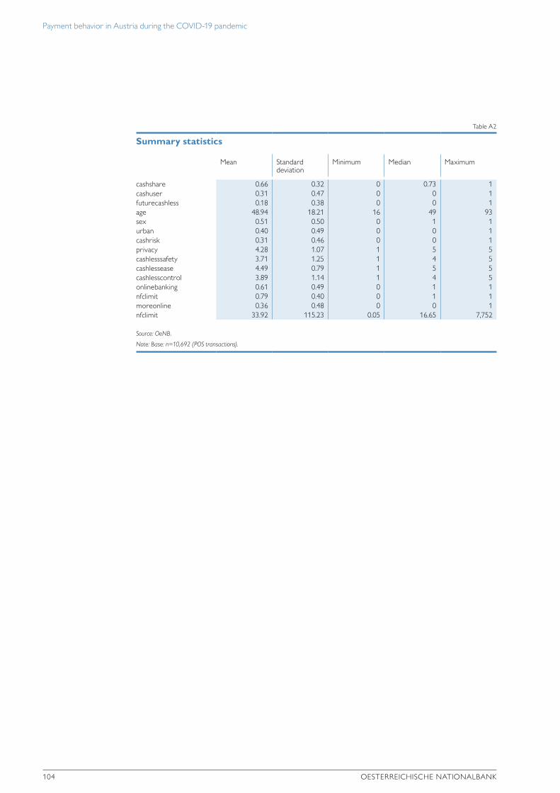
Payment behavior in Austria during the COVID-19 pandemic
104 OESTERREICHISCHE NATIONALBANK
Table A2
Summary statistics
Mean Standard deviation
Minimum Median Maximum
cashshare 0.66 0.32 0 0.73 1 cashuser 0.31 0.47 0 0 1 futurecashless 0.18 0.38 0 0 1 age 48.94 18.21 16 49 93 sex 0.51 0.50 0 1 1 urban 0.40 0.49 0 0 1 cashrisk 0.31 0.46 0 0 1 privacy 4.28 1.07 1 5 5 cashlesssafety 3.71 1.25 1 4 5 cashlessease 4.49 0.79 1 5 5 cashlesscontrol 3.89 1.14 1 4 5 onlinebanking 0.61 0.49 0 1 1 nfclimit 0.79 0.40 0 1 1 moreonline 0.36 0.48 0 0 1 nfclimit 33.92 115.23 0.05 16.65 7,752
Source: OeNB.
Note: Base: n=10,692 (POS transactions).

Economic outlook for Austria

MONETARY POLICY & THE ECONOMY Q4/21 107
Strong economic rebound amid high uncertainty about impact of Omicron variantEconomic outlook for Austria from 2021 to 2024 (December 2021)
Friedrich Fritzer, Doris Prammer, Mirjam Salish, Martin Schneider and Richard Sellner1
Cutoff date: December 9, 2021
In the course of 2021, the Austrian economy recovered more strongly than expected from the sharp contraction recorded in 2020. With the onset of the fourth wave of COVID-19 infections, however, this rebound will slow down again in late 2021 and early 2022. GDP growth for 2021 as a whole will come to 4.9% and will only be affected slightly by the recent slowdown. In early 2022, growth will still be driven by the negative effects of the fourth wave on domestic tourism and by persistent global supply disruptions. Once these effects wear off, we expect the Austrian economy to recover quickly and expand by 4.3% in 2022. In 2023 and 2024, economic growth will decelerate to 2.6% and 1.8%, respectively. This means that in the f irst half of 2022, Austria’s economic output will reach pre-crisis levels and by the end of the forecast horizon, it will almost be back in line with its pre-crisis trend. The Austrian labor market recovered swiftly from the disruptions caused by the pandemic. In recent months, it actually recorded labor supply shortages. The unemployment rate as defined by Public Employment Service Austria (AMS) went down to 8.2% in 2021 after having risen to 10.1% in 2020. It is expected to decline to 6.0% by 2024. On the back of higher energy prices and global supply disruptions, HICP inflation increased to 2.7% in 2021. In 2022, it will climb further to 3.2%, spurred by energy price developments, the introduction of the CO2 tax as of July 1, 2022, and higher nonenergy commodity prices. With supply-side bottlenecks dissolving and energy prices subsiding, inflation will be down to 2.3% in 2023 and 2.0% in 2024. Thanks to the economic upturn, Austria’s budget deficit improved markedly in 2021, coming to 5.9% of GDP. For 2022, we expect it to decline further to 2.1% as the economy continues to recover and discretionary COVID-19-related measures will be discontinued. The eco-social tax reform will hardly impair Austria’s positive f iscal performance. Austria’s government debt ratio is expected to reach 75.5% in 2024, following a gradual decline from its historic high of 83.2% recorded in 2020.
1 Summary
1.1 Pandemic dominates economic performance in late 2021 and in early 2022
Initial progress in COVID-19 vaccination in Austria was swift in 2021. In the summer, the pandemic appeared to have been largely overcome. As the cold season approached, however, vaccination rates turned out to be too low, and vaccine protection began to wane for those vaccinated early on. The combination of these factors resulted in a pronounced fourth wave of COVID-19 infections which, in turn, prompted new containment measures that dampened economic activity.
1 Oesterreichische Nationalbank, Economic Analysis Division, [email protected], [email protected], [email protected], [email protected], [email protected]. With contributions from Gerhard Fenz, Ernest Gnan, Birgit Niessner, Beate Resch and Klaus Vondra.

Strong economic rebound amid high uncertainty about impact of Omicron variant
108 OESTERREICHISCHE NATIONALBANK
1.2 Global economy: supply disruptions and capacity constraints slow down worldwide recovery
Following a pandemic-induced slump in 2020, the global economy saw a strong rebound in 2021. Economic recovery differed markedly across regions, however. In the course of the year, supply disruptions and sharp rises in commodity and energy prices had an increasingly dampening effect, thereby driving inflation across large parts of the global economy.
1.3 Partial loss of 2021/22 winter season and resolution of supply disruptions determine Austrian exports
Strong global growth caused Austrian goods exports to clearly exceed pre-crisis levels by mid-2021 and to reach a historic peak. In the second half of the year, global supply disruptions dampened Austrian export activity, however. These disruptions are expected to resolve gradually from the second quarter of 2022 onward. The fourth wave of COVID-19 infections and German travel warnings for Austria put a heavy strain on Austrian tourism in the 2021/22 winter season. As a consequence, we expect overnight stays by foreign tourists to decline by 50% against pre-crisis levels. Driven by catch-up processes, exports of goods and services grew strongly, by 10.5%, in 2021. For the years from 2022 to 2024, we expect export growth rates of 3.2%, 4.5% and 2.4%, respectively.
1.4 Lockdown postpones recovery of private consumption
The strong influence of the pandemic on private consumption in Austria persisted in 2021. While consumer spending picked up strongly in the summer, following the third lockdown, this uptrend was interrupted by the fourth wave of COVID-19 infections and the related containment measures. Growing at a rate of 1.8% in 2021, private consumption will only be able to offset parts of its 2020 slump. A 5.7% rise in household spending following the fourth lockdown in November and December 2021 will support domestic growth in 2022. Another important factor apart from households meeting pent-up demand and reducing the excess savings accumulated during the pandemic will be the current Austrian tax reform. In 2023 and 2024, consumption growth will remain robust at 3.4% and 2.4%, respectively.
Change on previous quarter in % (seasonally and working day-adjusted)
Real GDP growth
12
10
8
6
4
2
0
–2
–4
–6
–8
–10
–12
Annual change in %
Harmonised Index of Consumer Prices (HICP)
5
4
3
2
1
0
%
Unemployment rate (national definition)
14
12
10
8
6
4
2
0
OeNB December 2021 outlook for Austria – main results
Chart 1
Source: WIFO, Statistics Austria, OeNB December 2021 outlook.
Change on previous quarter or year in % Annual rate (of increase)2024
2020
6.8
4.94.3
2.61.8
2023202220212020
1.4
2.73.2
2.32.0
10.1
8.2
6.7 6.2 6.0
2021 2022 2023 2024
2020 2021 2022 2023 2024

Strong economic rebound amid high uncertainty about impact of Omicron variant
MONETARY POLICY & THE ECONOMY Q4/21 109
1.5 Expiration of investment premium will dampen investment growth from 2022 onward
Investment had already recovered in the second half of 2020 after a steep decline during the first lockdown. On the back of robust industrial production and supported by the investment premium instrument, investment in Austria grew by 5.7% in 2021, thus exceeding 2019 levels. When this instrument is discontinued and export dynamics weaken, the investment cycle will be slowing down visibly in response.
1.6 Labor market largely unaffected by fourth lockdown
In 2020, the short-time work scheme played a key role in stabilizing the labor market. As the recovery picked up speed, this instrument began to be used less frequently. 2021 saw employment expanding vigorously while skill shortages became more pronounced and the number of job vacancies reached record highs. Given its short duration, the fourth nation-wide lockdown did not have any signif-icant effects on employment and unemployment in Austria. The unemployment rate (national definition) decreased to 8.2% in 2021, down from a previous rate of 10.1%. We expect it to decline further to 6.0% by 2024 and thus to drop to a level significantly below the pre-crisis rate of 7.4% in 2019. The unemployment rate as
1.2 Global economy: supply disruptions and capacity constraints slow down worldwide recovery
Following a pandemic-induced slump in 2020, the global economy saw a strong rebound in 2021. Economic recovery differed markedly across regions, however. In the course of the year, supply disruptions and sharp rises in commodity and energy prices had an increasingly dampening effect, thereby driving inflation across large parts of the global economy.
1.3 Partial loss of 2021/22 winter season and resolution of supply disruptions determine Austrian exports
Strong global growth caused Austrian goods exports to clearly exceed pre-crisis levels by mid-2021 and to reach a historic peak. In the second half of the year, global supply disruptions dampened Austrian export activity, however. These disruptions are expected to resolve gradually from the second quarter of 2022 onward. The fourth wave of COVID-19 infections and German travel warnings for Austria put a heavy strain on Austrian tourism in the 2021/22 winter season. As a consequence, we expect overnight stays by foreign tourists to decline by 50% against pre-crisis levels. Driven by catch-up processes, exports of goods and services grew strongly, by 10.5%, in 2021. For the years from 2022 to 2024, we expect export growth rates of 3.2%, 4.5% and 2.4%, respectively.
1.4 Lockdown postpones recovery of private consumption
The strong influence of the pandemic on private consumption in Austria persisted in 2021. While consumer spending picked up strongly in the summer, following the third lockdown, this uptrend was interrupted by the fourth wave of COVID-19 infections and the related containment measures. Growing at a rate of 1.8% in 2021, private consumption will only be able to offset parts of its 2020 slump. A 5.7% rise in household spending following the fourth lockdown in November and December 2021 will support domestic growth in 2022. Another important factor apart from households meeting pent-up demand and reducing the excess savings accumulated during the pandemic will be the current Austrian tax reform. In 2023 and 2024, consumption growth will remain robust at 3.4% and 2.4%, respectively.
Change on previous quarter in % (seasonally and working day-adjusted)
Real GDP growth
12
10
8
6
4
2
0
–2
–4
–6
–8
–10
–12
Annual change in %
Harmonised Index of Consumer Prices (HICP)
5
4
3
2
1
0
%
Unemployment rate (national definition)
14
12
10
8
6
4
2
0
OeNB December 2021 outlook for Austria – main results
Chart 1
Source: WIFO, Statistics Austria, OeNB December 2021 outlook.
Change on previous quarter or year in % Annual rate (of increase)2024
2020
6.8
4.94.3
2.61.8
2023202220212020
1.4
2.73.2
2.32.0
10.1
8.2
6.7 6.2 6.0
2021 2022 2023 2024
2020 2021 2022 2023 2024

Strong economic rebound amid high uncertainty about impact of Omicron variant
110 OESTERREICHISCHE NATIONALBANK
defined by Eurostat is expected to decrease from 6.3% in 2021 to 4.7% in 2024. A comparison with pre-crisis figures is not useful here because of changes in the underlying methodology.
1.7 Wages increase in line with inflation and productivity
Reflecting the pronounced economic upswing around mid-2021 and rising inflation in the second half of the year, the fall round of wage settlement negotiations ended with a 3.2% rise, on average, of collectively agreed wages for 2022. For 2023 and 2024, collective wage growth is expected to slow down to 3.1% and 2.7%, respec-tively. This means that cumulated wage growth for the period from 2021 to 2024 corresponds to the sum of cumulated productivity growth and cumulated inflation. Therefore, wage growth will not generate additional pressure on prices over the forecast horizon.
1.8 Energy price-induced inflationary pressure will ease in late 2022
Inflation has accelerated significantly in 2021 to date on the back of energy price developments and global supply disruptions. For 2021 as a whole, HICP inflation will come to 2.7%. In 2022, it will climb further to 3.2%, mirroring the pass-through to end users of higher wholesale prices for gas and electricity, the introduction of the CO2 tax as of July 1, 2022, as well as rises in nonenergy commodity prices. In 2023 and 2024, inflation will slow down to 2.3% and 2.0%, respectively, as supply- side bottlenecks dissolve and energy futures prices will decline.
1.9 Budget deficit back below 3% of GDP in 2022
Thanks to the economic recovery, the Austrian budget deficit improved substan-tially in 2021 against 2020 figures. It still remains elevated, however, at 5.9% of GDP. With recovery progressing and discretionary COVID-19-related measures being discontinued, the budget deficit is expected to contract to 2.1% already in 2022 and thus to drop clearly below the Maastricht deficit threshold of 3%. The ecological and socially balanced (“eco-social”) tax reform, which will start to take effect in 2022, will hardly impair the positive course of Austria’s fiscal performance. On the back of high economic growth, Austria’s government debt ratio will, already in 2021, decline slightly from the historic high of 83.2% of GDP recorded in 2020. It will then decrease continuously to 75.5% of GDP in 2024.
Table 1
OeNB December 2021 outlook for Austria – main results1
2020 2021 2022 2023 2024
Economic activity Annual change in % (real)
Gross domestic product (GDP) –6.8 +4.9 +4.3 +2.6 +1.8Private consumption –8.4 +1.8 +5.7 +3.4 +2.4Government consumption –0.4 +5.3 –0.9 +0.3 +0.7Gross fixed capital formation –5.0 +5.7 +2.7 +1.9 +1.3Exports of goods and services –11.5 +10.5 +3.2 +4.8 +2.5Imports of goods and services –9.3 +11.3 +1.9 +4.5 +2.4
% of nominal GDP
Current account balance 1.9 –1.3 –0.5 1.0 1.3
Import-adjusted contributions to real GDP growth2 Percentage points
Private consumption –3.2 +0.6 +2.0 +1.2 +0.8Government consumption –0.1 +0.9 –0.2 +0.0 +0.1Gross fixed capital formation –0.7 +0.8 +0.4 +0.3 +0.2Domestic demand (excluding changes in inventories) –4.0 +2.3 +2.2 +1.5 +1.2Exports –3.6 +2.9 +0.9 +1.4 +0.8Changes in inventories (including statistical discrepancy) +0.4 +0.9 +0.0 +0.0 +0.0
Prices Annual change in %
Harmonised Index of Consumer Prices (HICP) +1.4 +2.7 +3.2 +2.3 +2.0Private consumption expenditure deflator +1.4 +2.5 +2.9 +2.2 +2.0GDP deflator +2.3 +2.3 +2.3 +2.5 +1.9Unit labor costs (whole economy) +7.7 –0.2 +0.9 +2.0 +1.6Compensation per employee (nominal) +1.9 +3.0 +3.5 +3.3 +2.6Compensation per hour worked (nominal) +10.4 –1.9 +2.8 +2.1 +2.5Import prices –1.8 +4.9 +3.9 +1.8 +1.9Export prices –0.8 +2.6 +2.8 +2.3 +1.8Terms of trade +1.0 –2.2 –1.1 +0.4 –0.1
Income and savings
Real disposable household income –2.0 –2.8 +3.3 +3.6 +2.5
% of nominal disposable household income
Saving ratio 14.3 9.6 7.1 7.3 7.4
Labor market Annual change in %
Payroll employment –2.0 +1.6 +1.7 +1.4 +0.8Hours worked (payroll employment) –9.4 +6.4 +2.4 +2.5 +0.9
% of labor supply
Unemployment rate (Eurostat definition) 6.1 6.3 5.4 5.0 4.7 Unemployment rate (national definition) 10.1 8.2 6.7 6.2 6.0
Public finances % of nominal GDP
Budget balance –8.3 –5.9 –2.1 –1.4 –1.1 Government debt 83.2 82.7 79.5 77.0 75.5
Source: 2020: Statistics Austria; 2021 to 2024: OeNB December 2021 outlook.1 This outlook was drawn up on the basis of seasonally and working day-adjusted national accounts data (as available for Q3 21). 2 The import-adjusted growth contributions were calculated by offsetting each final demand component with the corresponding imports, which were
obtained from input-output tables.

Strong economic rebound amid high uncertainty about impact of Omicron variant
MONETARY POLICY & THE ECONOMY Q4/21 111
defined by Eurostat is expected to decrease from 6.3% in 2021 to 4.7% in 2024. A comparison with pre-crisis figures is not useful here because of changes in the underlying methodology.
1.7 Wages increase in line with inflation and productivity
Reflecting the pronounced economic upswing around mid-2021 and rising inflation in the second half of the year, the fall round of wage settlement negotiations ended with a 3.2% rise, on average, of collectively agreed wages for 2022. For 2023 and 2024, collective wage growth is expected to slow down to 3.1% and 2.7%, respec-tively. This means that cumulated wage growth for the period from 2021 to 2024 corresponds to the sum of cumulated productivity growth and cumulated inflation. Therefore, wage growth will not generate additional pressure on prices over the forecast horizon.
1.8 Energy price-induced inflationary pressure will ease in late 2022
Inflation has accelerated significantly in 2021 to date on the back of energy price developments and global supply disruptions. For 2021 as a whole, HICP inflation will come to 2.7%. In 2022, it will climb further to 3.2%, mirroring the pass-through to end users of higher wholesale prices for gas and electricity, the introduction of the CO2 tax as of July 1, 2022, as well as rises in nonenergy commodity prices. In 2023 and 2024, inflation will slow down to 2.3% and 2.0%, respectively, as supply- side bottlenecks dissolve and energy futures prices will decline.
1.9 Budget deficit back below 3% of GDP in 2022
Thanks to the economic recovery, the Austrian budget deficit improved substan-tially in 2021 against 2020 figures. It still remains elevated, however, at 5.9% of GDP. With recovery progressing and discretionary COVID-19-related measures being discontinued, the budget deficit is expected to contract to 2.1% already in 2022 and thus to drop clearly below the Maastricht deficit threshold of 3%. The ecological and socially balanced (“eco-social”) tax reform, which will start to take effect in 2022, will hardly impair the positive course of Austria’s fiscal performance. On the back of high economic growth, Austria’s government debt ratio will, already in 2021, decline slightly from the historic high of 83.2% of GDP recorded in 2020. It will then decrease continuously to 75.5% of GDP in 2024.
Table 1
OeNB December 2021 outlook for Austria – main results1
2020 2021 2022 2023 2024
Economic activity Annual change in % (real)
Gross domestic product (GDP) –6.8 +4.9 +4.3 +2.6 +1.8Private consumption –8.4 +1.8 +5.7 +3.4 +2.4Government consumption –0.4 +5.3 –0.9 +0.3 +0.7Gross fixed capital formation –5.0 +5.7 +2.7 +1.9 +1.3Exports of goods and services –11.5 +10.5 +3.2 +4.8 +2.5Imports of goods and services –9.3 +11.3 +1.9 +4.5 +2.4
% of nominal GDP
Current account balance 1.9 –1.3 –0.5 1.0 1.3
Import-adjusted contributions to real GDP growth2 Percentage points
Private consumption –3.2 +0.6 +2.0 +1.2 +0.8Government consumption –0.1 +0.9 –0.2 +0.0 +0.1Gross fixed capital formation –0.7 +0.8 +0.4 +0.3 +0.2Domestic demand (excluding changes in inventories) –4.0 +2.3 +2.2 +1.5 +1.2Exports –3.6 +2.9 +0.9 +1.4 +0.8Changes in inventories (including statistical discrepancy) +0.4 +0.9 +0.0 +0.0 +0.0
Prices Annual change in %
Harmonised Index of Consumer Prices (HICP) +1.4 +2.7 +3.2 +2.3 +2.0Private consumption expenditure deflator +1.4 +2.5 +2.9 +2.2 +2.0GDP deflator +2.3 +2.3 +2.3 +2.5 +1.9Unit labor costs (whole economy) +7.7 –0.2 +0.9 +2.0 +1.6Compensation per employee (nominal) +1.9 +3.0 +3.5 +3.3 +2.6Compensation per hour worked (nominal) +10.4 –1.9 +2.8 +2.1 +2.5Import prices –1.8 +4.9 +3.9 +1.8 +1.9Export prices –0.8 +2.6 +2.8 +2.3 +1.8Terms of trade +1.0 –2.2 –1.1 +0.4 –0.1
Income and savings
Real disposable household income –2.0 –2.8 +3.3 +3.6 +2.5
% of nominal disposable household income
Saving ratio 14.3 9.6 7.1 7.3 7.4
Labor market Annual change in %
Payroll employment –2.0 +1.6 +1.7 +1.4 +0.8Hours worked (payroll employment) –9.4 +6.4 +2.4 +2.5 +0.9
% of labor supply
Unemployment rate (Eurostat definition) 6.1 6.3 5.4 5.0 4.7 Unemployment rate (national definition) 10.1 8.2 6.7 6.2 6.0
Public finances % of nominal GDP
Budget balance –8.3 –5.9 –2.1 –1.4 –1.1 Government debt 83.2 82.7 79.5 77.0 75.5
Source: 2020: Statistics Austria; 2021 to 2024: OeNB December 2021 outlook.1 This outlook was drawn up on the basis of seasonally and working day-adjusted national accounts data (as available for Q3 21). 2 The import-adjusted growth contributions were calculated by offsetting each final demand component with the corresponding imports, which were
obtained from input-output tables.

Strong economic rebound amid high uncertainty about impact of Omicron variant
112 OESTERREICHISCHE NATIONALBANK
2 Assumptions
2.1 General assumptions
This outlook for the Austrian economy is the OeNB’s contribution to the December 2021 Eurosystem staff macroeconomic projections. The forecast horizon ranges from the fourth quarter of 2021 to the fourth quarter of 2024. The cutoff date for all assumptions on global economic performance, interest rates, exchange rates and crude oil prices was November 26, 2021. This outlook was prepared on the basis of the OeNB’s macroeconomic quarterly model. The seasonally and working day-adjusted national accounts data calculated by Statistics Austria were available up to and including the third quarter of 2021.
2.2 Global economy: supply disruptions and capacity constraints slow down worldwide recovery
In 2021, the global economy recovered from the effects of the first waves of the COVID-19 pandemic in 2020. In the course of the year, however, the recovery lost some of its momentum and became increasingly heterogeneous. While economic activity has meanwhile reached pre-crisis levels or levels just below pre-crisis levels in most developed economies, low vaccination rates in many developing economies make them a lot more vulnerable to the pandemic. With the significantly more infectious Delta variant of the coronavirus spreading around the globe, however, new waves of infections also occurred in the developed economies. In the USA, for instance, the current wave already peaked in August 2021. In the United Kingdom, the number of new infections has been at elevated levels since the summer, and the countries of the European Union have been hit by the fourth wave of the pandemic since the fall, albeit to differing degrees. The situation differs significantly also within individual economies. High-contact sectors and low-income households have felt the impact of containment measures most strongly. By expanding global vaccine production, it should become possible to reduce the economic and social impact of the pandemic substantially. Rising vaccination rates would help contain the spreading of the coronavirus; in addition, disease progression would be mitigated, which means that the number of hospitalizations and deaths would go down and, consequently, containment measures could be reduced. In this context, the new Omicron variant constitutes a substantial risk factor as it is highly contagious.
In the course of 2021, the supply of commodities and goods was not able to keep up with the strong rise in demand during the economic recovery. Apart from hikes in crude oil and natural gas prices, the prices of industrial metals soared as well. Global value chains were affected by disruptions of major transport nodes (Suez Canal obstruction, closure of Chinese ports, etc.), which led to considerable price increases within production processes and to interruptions in production. Moreover, inflation was spurred by rising prices for CO2 certificates. Rising inflation rates prompted debates on an unwinding of accommodative monetary policies in a number of economies.
Backed by vigorous consumption growth, the US economy expanded strongly in the first half of 2021. Meanwhile, most fiscal support measures (e.g. stimulus checks) have been discontinued. Savings accumulated during the pandemic will continue to support consumption also in the near future. In the third quarter of 2021, a new wave of the COVID-19 pandemic and supply bottlenecks put a brake on economic

Strong economic rebound amid high uncertainty about impact of Omicron variant
MONETARY POLICY & THE ECONOMY Q4/21 113
activity in the United States. Consumer price inflation accelerated considerably throughout 2021 and came to 6.2% in October. The country’s vaccination rate, which is low compared with rates in most other advanced economies, might continue to dampen recovery during the winter of 2021/22. While the labor market has been recovering noticeably, labor participation is still around 2 percentage points below pre-pandemic levels. In November 2021, consumer confidence hit the lowest level since the financial crisis of 2008 and 2009. Rising inflation, in particular with regard to real estate, consumer goods and vehicles, was quoted as the main reason for the decrease in consumer confidence. In early November 2021, the US Federal Reserve announced the gradual tapering of its government bond purchase program; purchases are to be wound down by June 2022. The fiscal packages adopted by the Biden administration will provide a major growth stimulus in the coming years.
Economic growth in China will come to just under 8.0% in 2021, relying on strongly expanding exports as the main driver of growth even though the pace of expansion slowed down in the course of the year. This deceleration is not least due to the zero-COVID-19 strategy adopted by the Chinese government, which implies that production sites and ports are closed down when even a single person is diag-nosed with COVID-19. Over the last few months, the Chinese government has significantly tightened regulations concerning both the real estate sector and lending. The looming insolvency of the real estate group Evergrande constitutes a perceptible risk, given the group’s size and possible contagion effects. The fact that production
Table 2
Underlying global economic conditions
2020 2021 2022 2023 2024
Gross domestic product Annual change in % (real)
World excluding the euro area –2.3 +6.0 +4.5 +3.9 +3.7USA –3.4 +5.5 +4.2 +3.0 +2.5China +2.2 +7.9 +5.0 +5.3 +5.3 India –7.1 +7.1 +8.3 +7.1 +6.9 Japan –4.7 +1.7 +2.6 +1.3 +1.0Latin America –7.2 +6.9 +2.8 +2.7 +2.5United Kingdom –9.7 +6.9 +4.0 +1.6 +1.2CESEE EU member states1 –3.8 +5.2 +4.2 +3.4 +3.3Switzerland –2.5 +2.9 +2.5 +1.9 +1.9Euro area2 –6.5 +5.1 +4.2 +2.9 +1.6
World trade (imports of goods and services)World –8.3 +10.2 +4.5 +4.9 +3.7World excluding the euro area –8.0 +11.1 +3.9 +4.4 +4.0Growth of euro area export markets (real) –9.3 +8.9 +4.0 +4.3 +3.9Growth of Austrian export markets (real) –8.9 +8.5 +5.0 +6.5 +3.2
Prices Absolute figures
Oil price in USD/barrel (Brent) 41.5 71.8 77.5 72.3 69.4 Three-month interest rate in % –0.4 –0.5 –0.5 –0.2 0.0 Long-term interest rate in % –0.2 –0.1 0.2 0.3 0.5 USD/EUR exchange rate 1.1 1.2 1.1 1.1 1.1 Nominal effective exchange rate of the euro (euro area index) 119.3 120.7 118.3 118.3 118.3
Source: Eurosystem.1 Bulgaria, Croatia, Czechia, Hungary, Poland and Romania. 2 2020: Eurostat; 2021 to 2024: results of the Eurosystem’s December 2021 projections.
Strong economic rebound amid high uncertainty about impact of Omicron variant
114 OESTERREICHISCHE NATIONALBANK
sites had to be closed down because of energy shortages also contributed to the slowdown in growth dynamics.
India witnessed a 12% slump in economic performance in the second quarter of 2021 as a result of a massive wave of COVID-19 infections and the drastic con-tainment measures taken to combat it; in the third quarter, however, as restrictions were loosened, the economy largely recovered. We expect growth in India to come to 7.4% in 2021 and 8.9% in 2022. The Russian economy is fueled by private consumption and the strong global demand for commodities, which has caused prices to climb. Recovery across the other transition economies differs widely.
The United Kingdom lifted most of its pandemic-related restrictions in July 2021, given high vaccination coverage. These steps supported private consumption. Growth dynamics have been losing momentum in the second half of 2021, however. What burdens the UK economy apart from global supply disruptions are pronounced labor shortages resulting from the country’s withdrawal from the European Union. The lack of workers is most apparent in transportation and the catering and restau-rant sector. Even though growth will slow down in 2022 compared with 2021 (+6.9%), it will continue at a high level of 4.0%.
As in 2020, the pandemic and its economic implications continued to dominate the situation in the euro area in 2021. The containment measures implemented in many euro area countries in the winter of 2020/21 caused households’ consumer spending to decline. While demand for services went down, industry and the construction sector expanded noticeably. The broad-based lifting of containment measures in many euro area countries in spring 2021 caused private consumption to rise sharply in the second and third quarters, based on significant labor market improvements and declining saving ratios. Industrial activity slowed down, however, mainly due to supply-side bottlenecks and a strong increase in the prices for energy and commodities. Again, developments differed widely across countries.
Economic developments in Germany are largely connected to the size and struc-ture of the country’s industrial sector. While export orders reached historic highs, industrial production has been decreasing continuously since the fourth quarter of 2020 because of supply disruptions. Most prominently, the shortage of microchips caused production sites to be closed down in the automotive industry, a major pillar of German industry. While the current wave of COVID-19 infections hit Germany later than Austria, it is still expected to impair economic activity in the winter of 2021/22. For 2021 as a whole, growth in Germany will remain moderate. For 2022, we expect a robust recovery which, in combination with growing labor shortages, will lead to a further rise in inflation rates. Fueled by robust investment activity and strong consumer demand, the French economy was a lot more dynamic in 2021 than the German economy. Consumption growth will peak in 2022 on the basis of favorable labor market developments while the investment cycle will be nearing completion. GDP growth will reach pre-crisis levels as the pace of export growth moderates. Italy recorded an above-average economic slump in 2020 when compared to its euro area peers. The ensuing upturn was backed essentially by a comprehensive fiscal package. In Spain, the economic impact of the pandemic was particularly strong in 2020, with GDP contracting more sharply than in any other euro area country. Given the country’s very high vaccination coverage, however, the current wave of COVID-19 infections has been mild by comparison; still, the number of foreign tourists during the summer season was no more than about half of pre-crisis figures.
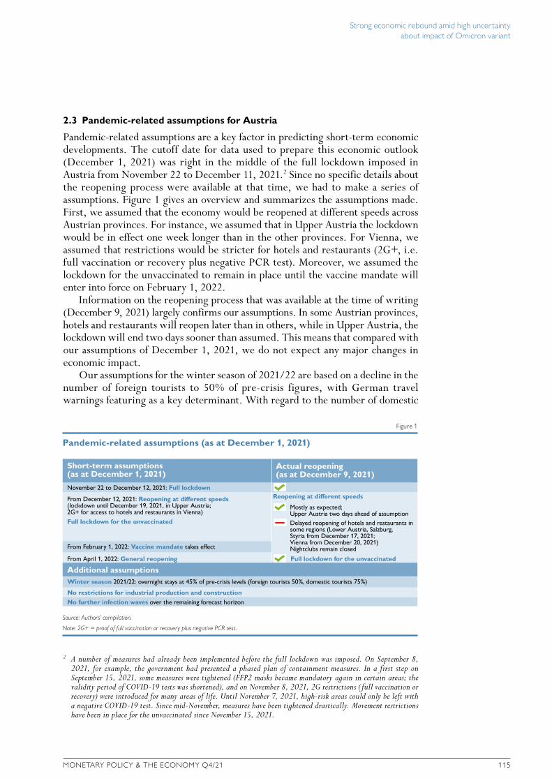
Strong economic rebound amid high uncertainty about impact of Omicron variant
MONETARY POLICY & THE ECONOMY Q4/21 115
2.3 Pandemic-related assumptions for Austria
Pandemic-related assumptions are a key factor in predicting short-term economic developments. The cutoff date for data used to prepare this economic outlook (December 1, 2021) was right in the middle of the full lockdown imposed in Austria from November 22 to December 11, 2021.2 Since no specific details about the reopening process were available at that time, we had to make a series of assumptions. Figure 1 gives an overview and summarizes the assumptions made. First, we assumed that the economy would be reopened at different speeds across Austrian provinces. For instance, we assumed that in Upper Austria the lockdown would be in effect one week longer than in the other provinces. For Vienna, we assumed that restrictions would be stricter for hotels and restaurants (2G+, i.e. full vaccination or recovery plus negative PCR test). Moreover, we assumed the lockdown for the unvaccinated to remain in place until the vaccine mandate will enter into force on February 1, 2022.
Information on the reopening process that was available at the time of writing (December 9, 2021) largely confirms our assumptions. In some Austrian provinces, hotels and restaurants will reopen later than in others, while in Upper Austria, the lockdown will end two days sooner than assumed. This means that compared with our assumptions of December 1, 2021, we do not expect any major changes in economic impact.
Our assumptions for the winter season of 2021/22 are based on a decline in the number of foreign tourists to 50% of pre-crisis figures, with German travel warnings featuring as a key determinant. With regard to the number of domestic
2 A number of measures had already been implemented before the full lockdown was imposed. On September 8, 2021, for example, the government had presented a phased plan of containment measures. In a first step on September 15, 2021, some measures were tightened (FFP2 masks became mandatory again in certain areas; the validity period of COVID-19 tests was shortened), and on November 8, 2021, 2G restrictions ( full vaccination or recovery) were introduced for many areas of life. Until November 7, 2021, high-risk areas could only be left with a negative COVID-19 test. Since mid-November, measures have been tightened drastically. Movement restrictions have been in place for the unvaccinated since November 15, 2021.
Pandemic-related assumptions (as at December 1, 2021)
Figure 1
Source: Authors’ compilation.
Note: 2G+ = proof of full vaccination or recovery plus negative PCR test.
Short-term assumptions (as at December 1, 2021)
Actual reopening(as at December 9, 2021)
November 22 to December 12, 2021: Full lockdown
From December 12, 2021: Reopening at different speeds(lockdown until December 19, 2021, in Upper Austria; 2G+ for access to hotels and restaurants in Vienna)
Reopening at different speeds
Full lockdown for the unvaccinated
Mostly as expected; Upper Austria two days ahead of assumptionDelayed reopening of hotels and restaurants in some regions (Lower Austria, Salzburg, Styria from December 17, 2021; Vienna from December 20, 2021)Nightclubs remain closedFrom February 1, 2022: Vaccine mandate takes effect
From April 1, 2022: General reopening Full lockdown for the unvaccinated
Additional assumptions
No restrictions for industrial production and constructionNo further infection waves over the remaining forecast horizon
Winter season 2021/22: overnight stays at 45% of pre-crisis levels (foreign tourists 50%, domestic tourists 75%)

Strong economic rebound amid high uncertainty about impact of Omicron variant
116 OESTERREICHISCHE NATIONALBANK
tourists, we assume a 75% decline. Moreover, we assume that like during the second and third lockdowns, there will not be any restrictions to industry and the construction sector. For the remainder of the forecast horizon, we assume that there will not be any further large-scale waves of COVID-19 infections.
3 Exports and consumption drive economic growth
3.1 Partial loss of 2021/22 winter season and resolution of supply disruptions determine Austrian exports
The first lockdown in spring 2020 affected not only high-contact services but also the output of export-oriented industries. In the second quarter of 2020, Austrian exports of goods and services contracted by 22.5% year on year in real terms. While tourism exports continued to feel the impact of the pandemic during subse-quent quarters, goods exports already recovered in the third quarter of 2020 on the back of high international demand. In 2020 as a whole, total exports went down by 11.5%, with services exports declining by twice as much (–17.8%) as goods exports (–8.6%). Strong global growth caused Austrian goods exports to exceed pre-crises levels (i.e. Q4 19 figures) by 9% in the second quarter of 2021 and to reach a historic peak. In the second half of 2021, the effects of global supply disruptions began to show. The close economic ties of Austrian exporters with German industry acted as an aggravating factor, and real goods exports declined in the third quarter of 2021. If the global supply disruptions resolve during 2022 as assumed, goods exports will recover gradually. What will be decisive in this respect is the expected rise in import demand by the German industrial sector.
The fourth wave of the pandemic and the related containment measures place a heavy burden on Austrian tourism, also in the 2021/22 winter season. The outlook for the Austrian winter tourist season is affected in particular by the travel warnings and other containment measures in place in Germany. Under the assumption of a cautious reopening at different speeds in different regions, we do not expect the winter season to be a total loss (like in 2020/21); instead, we assume that the number of overnight stays by foreign tourists will decline by 50% against pre-crisis levels. For 2021 as a whole, we thus expect exports of goods and services to expand by 10.5%.
In the first quarter of 2022, the combined effect of the expected partial loss of the winter season and the dampening of goods exports by bottlenecks in supply will cause a further decline in total exports. In the second quarter of 2022, export dynamics will gain speed as tourism will recover and supply disruptions start resolving. In 2022 as a whole, export growth will be considerably weaker, at 3.2%, than in 2021; this moderation will be attributable to a slowdown in the second half of 2021 and the related negative carry-over effect in combination with a weak performance in the first quarter of 2022. In 2023, Austrian exports will expand by 4.8% before the export cycle will near its end in 2024 (+2.5%).
The total loss of the 2020/21 winter tourist season left its mark on Austria’s current account. The balance on the travel account deteriorated markedly in the first half of 2021, posting a surplus of no more than EUR 340 million – down from EUR 6.3 billion in the first half of 2019. This contraction affects the balance of services, whose surplus will shrink from 2.1% of GDP in 2020 to 0.4% in 2021. While we expect some improvement in 2022, the surplus on the services balance will come to no more than 1.5% of GDP and will thus remain clearly below the
Table 3
Austria’s exports and imports and price competitiveness
2020 2021 2022 2023 2024
Exports Annual change in %
Competitor prices on Austria’s export markets –2.4 +6.7 +5.4 +1.2 +1.3Export deflator –0.8 +2.6 +2.8 +2.3 +1.8Changes in price competitiveness1 –1.7 +4.1 +2.6 –1.1 –0.5Import demand on Austria’s export markets (real) –8.9 +8.5 +5.0 +6.5 +3.2Austrian exports of goods and services (real) –11.5 +10.5 +3.2 +4.8 +2.5Austrian market share –2.5 +2.1 –1.8 –1.6 –0.7
Imports Annual change in %
International competitor prices on the Austrian market –1.6 +5.9 +5.4 +1.3 +1.4Import deflator –1.8 +4.9 +3.9 +1.8 +1.9Austrian imports of goods and services (real) –9.3 +11.3 +1.9 +4.5 +2.4
Terms of trade +1.0 –2.2 –1.1 +0.4 –0.1
Percentage points of real GDP
Contribution of net exports to GDP growth –1.6 –0.1 +0.8 +0.4 +0.2
% of nominal GDP
Export ratio 51.2 54.1 53.8 54.9 55.2 Import ratio 48.6 52.9 52.5 53.1 53.4
Source: 2020: Statistics Austria, Eurosystem; 2021 to 2024: OeNB December 2021 outlook.1 Changes in price competitiveness are defined as the difference between changes in competitor prices on Austria’s export markets and changes in
the export deflator.
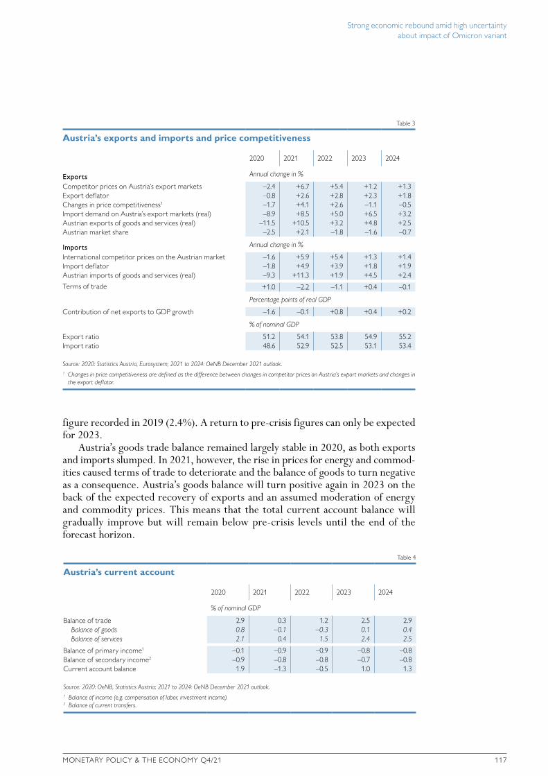
Strong economic rebound amid high uncertainty about impact of Omicron variant
MONETARY POLICY & THE ECONOMY Q4/21 117
figure recorded in 2019 (2.4%). A return to pre-crisis figures can only be expected for 2023.
Austria’s goods trade balance remained largely stable in 2020, as both exports and imports slumped. In 2021, however, the rise in prices for energy and commod-ities caused terms of trade to deteriorate and the balance of goods to turn negative as a consequence. Austria’s goods balance will turn positive again in 2023 on the back of the expected recovery of exports and an assumed moderation of energy and commodity prices. This means that the total current account balance will gradually improve but will remain below pre-crisis levels until the end of the forecast horizon.
Table 4
Austria’s current account
2020 2021 2022 2023 2024
% of nominal GDP
Balance of trade 2.9 0.3 1.2 2.5 2.9 Balance of goods 0.8 –0.1 –0.3 0.1 0.4 Balance of services 2.1 0.4 1.5 2.4 2.5
Balance of primary income1 –0.1 –0.9 –0.9 –0.8 –0.8 Balance of secondary income2 –0.9 –0.8 –0.8 –0.7 –0.8 Current account balance 1.9 –1.3 –0.5 1.0 1.3
Source: 2020: OeNB, Statistics Austria; 2021 to 2024: OeNB December 2021 outlook.1 Balance of income (e.g. compensation of labor, investment income).2 Balance of current transfers.
tourists, we assume a 75% decline. Moreover, we assume that like during the second and third lockdowns, there will not be any restrictions to industry and the construction sector. For the remainder of the forecast horizon, we assume that there will not be any further large-scale waves of COVID-19 infections.
3 Exports and consumption drive economic growth
3.1 Partial loss of 2021/22 winter season and resolution of supply disruptions determine Austrian exports
The first lockdown in spring 2020 affected not only high-contact services but also the output of export-oriented industries. In the second quarter of 2020, Austrian exports of goods and services contracted by 22.5% year on year in real terms. While tourism exports continued to feel the impact of the pandemic during subse-quent quarters, goods exports already recovered in the third quarter of 2020 on the back of high international demand. In 2020 as a whole, total exports went down by 11.5%, with services exports declining by twice as much (–17.8%) as goods exports (–8.6%). Strong global growth caused Austrian goods exports to exceed pre-crises levels (i.e. Q4 19 figures) by 9% in the second quarter of 2021 and to reach a historic peak. In the second half of 2021, the effects of global supply disruptions began to show. The close economic ties of Austrian exporters with German industry acted as an aggravating factor, and real goods exports declined in the third quarter of 2021. If the global supply disruptions resolve during 2022 as assumed, goods exports will recover gradually. What will be decisive in this respect is the expected rise in import demand by the German industrial sector.
The fourth wave of the pandemic and the related containment measures place a heavy burden on Austrian tourism, also in the 2021/22 winter season. The outlook for the Austrian winter tourist season is affected in particular by the travel warnings and other containment measures in place in Germany. Under the assumption of a cautious reopening at different speeds in different regions, we do not expect the winter season to be a total loss (like in 2020/21); instead, we assume that the number of overnight stays by foreign tourists will decline by 50% against pre-crisis levels. For 2021 as a whole, we thus expect exports of goods and services to expand by 10.5%.
In the first quarter of 2022, the combined effect of the expected partial loss of the winter season and the dampening of goods exports by bottlenecks in supply will cause a further decline in total exports. In the second quarter of 2022, export dynamics will gain speed as tourism will recover and supply disruptions start resolving. In 2022 as a whole, export growth will be considerably weaker, at 3.2%, than in 2021; this moderation will be attributable to a slowdown in the second half of 2021 and the related negative carry-over effect in combination with a weak performance in the first quarter of 2022. In 2023, Austrian exports will expand by 4.8% before the export cycle will near its end in 2024 (+2.5%).
The total loss of the 2020/21 winter tourist season left its mark on Austria’s current account. The balance on the travel account deteriorated markedly in the first half of 2021, posting a surplus of no more than EUR 340 million – down from EUR 6.3 billion in the first half of 2019. This contraction affects the balance of services, whose surplus will shrink from 2.1% of GDP in 2020 to 0.4% in 2021. While we expect some improvement in 2022, the surplus on the services balance will come to no more than 1.5% of GDP and will thus remain clearly below the
Table 3
Austria’s exports and imports and price competitiveness
2020 2021 2022 2023 2024
Exports Annual change in %
Competitor prices on Austria’s export markets –2.4 +6.7 +5.4 +1.2 +1.3Export deflator –0.8 +2.6 +2.8 +2.3 +1.8Changes in price competitiveness1 –1.7 +4.1 +2.6 –1.1 –0.5Import demand on Austria’s export markets (real) –8.9 +8.5 +5.0 +6.5 +3.2Austrian exports of goods and services (real) –11.5 +10.5 +3.2 +4.8 +2.5Austrian market share –2.5 +2.1 –1.8 –1.6 –0.7
Imports Annual change in %
International competitor prices on the Austrian market –1.6 +5.9 +5.4 +1.3 +1.4Import deflator –1.8 +4.9 +3.9 +1.8 +1.9Austrian imports of goods and services (real) –9.3 +11.3 +1.9 +4.5 +2.4
Terms of trade +1.0 –2.2 –1.1 +0.4 –0.1
Percentage points of real GDP
Contribution of net exports to GDP growth –1.6 –0.1 +0.8 +0.4 +0.2
% of nominal GDP
Export ratio 51.2 54.1 53.8 54.9 55.2 Import ratio 48.6 52.9 52.5 53.1 53.4
Source: 2020: Statistics Austria, Eurosystem; 2021 to 2024: OeNB December 2021 outlook.1 Changes in price competitiveness are defined as the difference between changes in competitor prices on Austria’s export markets and changes in
the export deflator.

Strong economic rebound amid high uncertainty about impact of Omicron variant
118 OESTERREICHISCHE NATIONALBANK
3.2 Lockdown postpones recovery of private consumption
After the outbreak of the COVID-19 pandemic in 2020, real private consumption in Austria contracted by 8.3% and, given its high share in GDP, contributed essen-tially to the major economic downturn (–6.8%). The measures taken to contain the spreading of the coronavirus, such as the shutdown of retail outlets, hotels and restaurants, strongly limited consumer spending, in particular on close-contact or tourist services, and led to forced saving. At the same time, government support measures like the short-time work scheme prevented a sharp decline in real dispos-able household income (–2.0%). As a consequence, the saving ratio jumped by 5.8 percentage points to 14.3%.
During Austria’s second and third lockdowns (fall 2020 and winter 2020/21), household spending and disposable household income declined steadily in late 2020 and early 2021. As businesses began to reopen gradually, consumer spending recov-ered strongly, rising by 4.0% in the second and 7.0% in the third quarter of 2021 (quarter on quarter). Given the strong rise in the number of infections and the high occupancy of intensive care beds at Austrian hospitals during the fourth wave of the pandemic, the Austrian government imposed a fourth lockdown for an initial period of three weeks (November 22 to December 12, 2021). Preceding this had been a partial lockdown for unvaccinated persons from November 15 to November 21, 2021.
According to the weekly OeNB GDP indicator3, Austria’s economic output in this single week was about 2% higher than in the comparable week of 2019, i.e. higher than pre-crisis levels, and also higher than in the weeks before the partial lockdown. This rise was attributable in particular to higher retail sales, which implies that consumers were frontloading purchases in anticipation of a full lock-down. In the first week of the fourth lockdown, Austria’s economic output remained around 9% below pre-crisis levels, which translates into a EUR 700 mil-lion weekly loss in value added. This means that the decline in weekly output was considerably weaker than during the first lockdown in spring 2020 (–20% or –EUR 2 billion) and during the second and third lockdowns in the winter of 2020/21 (–12% or –EUR 900 million). The relatively moderate decline in output recorded during the fourth lockdown can be traced to two reasons. Measures imposed during the fourth lockdown have been limited to sectors directly affected by healthcare measures (like during the second and third lockdowns); unlike during the first lockdown, the current measures do not apply to manufacturing enter-prises and the construction sector. The sectors concerned also profit from their previous lockdown experience and have developed alternative sales channels such as click and collect, e-commerce or takeaway options. For these reasons, sales losses in retail trade and the hotel and restaurant business have been smaller than during previous lockdowns. In total, however, they are still considerable and account for just under three-quarters of the slump in Austria’s GDP, with the remainder being attributable to losses in tourism exports.
3 Weekly OeNB GDP indicator (detailed information in German, tables and charts also available in English): https://www.oenb.at/Publikationen/corona/bip-indikator-der-oenb.html.

Strong economic rebound amid high uncertainty about impact of Omicron variant
MONETARY POLICY & THE ECONOMY Q4/21 119
On the basis of these estimations, in preparing this outlook we assume that one week of the current lockdown4 will cause consumer spending to decline by EUR 525 million (= 75% * EUR 700 million). According to government announce-ments, the three-week full lockdown will be followed by a partial lockdown for the unvaccinated (comparable to the week preceding the fourth lockdown). To estimate the drop in consumption during one week of partial lockdown, we assume that this drop will not correspond to the share of unvaccinated persons in the total population, but will be lower. After all, measures might be bypassed to a degree, and purchases could be made by vaccinated persons instead. We therefore expect effects to be reduced by one-quarter. Starting from the assumption that one-third of the total population are not vaccinated, this means that one week of partial lock-down for the unvaccinated would translate into a decline in household consump-tion of around EUR 130 million (= EUR 525 million * ⅓ * ¼). As an additional containment measure, the Austrian government announced that vaccination will be mandatory as of February 1, 2022. We assume that as a result the share of unvaccinated persons in the total population will decline over the coming months. Moreover, we assume that the partial lockdown will remain in place until the end of January 2022 and that further restrictions will continue to apply for the unvac-cinated beyond January. All in all, these assumptions result in an expected decline in real household spending by 4.5% in the fourth quarter of 2021, followed by a 3.8% rise in the first quarter of 2022 as containment measures will be eased.
The future path of consumption will not only depend on the current containment measures but also on consumers’ use of excess savings accumulated during the pandemic. Schneider and Sellner (2021)5 estimate the volume of excess savings Austrian households accumulated between the first quarter of 2020 and the second quarter of 2021 to come to EUR 10.8 billion. Our outlook is based on the assumption that households will use one-third (EUR 3.6 billion) of this amount for consumption purposes in the second half of 2021 and in 2022.
In 2020, government support prevented household income from declining sharply. Over the forecast horizon, these transfer payments will be reduced in line with economic recovery, which means that developments in disposable household income will depend on the growth rate of employee compensation. In view of strong productivity growth and elevated inflation rates, the collective wage agree-ments concluded for 2022 were relatively high. In addition, the strong economic rebound and skill shortages contribute to growth via a positive wage drift. Moreover, the reduction of the tax rate in the second and third income brackets (as of July 2022 and July 2023, respectively) under the eco-social tax reform will strengthen people’s purchasing power. Compared with the 2016 tax reform, this reduction is small, however, and in addition, it will be minimized further by the unwinding of pandemic-related support measures.
4 To account for the extension of the lockdown in Upper Austria until December 19, 2021, as announced by the provincial government, we scaled the effects on consumption by Upper Austria’s share in Austrian value added (17.2%). For Vienna, we assume tighter restrictions for hotels and restaurants.
5 Schneider, M. and R. Sellner (2021). Private consumption and savings during the COVID-19 pandemic in Austria, in Monetary Policy and the Economy Q4/21.

Strong economic rebound amid high uncertainty about impact of Omicron variant
120 OESTERREICHISCHE NATIONALBANK
Capital income contracted sharply in 2020 as limits were imposed on profit distributions by enterprises that had received government support. After a brief recovery, this downtrend continued in early 2021, causing capital income to make a negative contribution to household income growth yet again. In total, nominal household income in Austria therefore declined somewhat in 2021. For 2022, we expect disposable household income to grow vigorously as capital income recovers; over the remaining forecast horizon, household income growth is set to slow down again.
In 2022, 2023 and 2024, overall disposable household income in Austria will augment by 3.3%, 3.6% and 2.5%, respectively. Real private consumption is expected to increase by no more than 1.8% in 2021 owing to the effects of the third and fourth lockdowns. It will only begin to recover fully in 2022 at a growth rate of 5.7%. After that, its pace will slow down to 3.4% in 2023 and 2.4% in 2024. Over the forecast horizon, private consumption will act as a key growth driver in Austria.
With businesses reopening and consumption recovering accordingly, savings from current income will be swift to reach pre-crisis levels. The partial reduction of excess savings accumulated during the pandemic will cause the saving ratio to fall below its pre-crisis level of 7.6% (2015 to 2019) temporarily before gradually resuming this level.
Table 5
Determinants of nominal household income and private consumption growth in Austria
2020 2021 2022 2023 2024
Annual change in %
Payroll employment –2.0 +1.6 +1.7 +1.4 +0.8Wages and salaries per employee +1.9 +3.0 +3.5 +3.3 +2.6Compensation of employees –0.1 +4.6 +5.3 +4.7 +3.5Investment income –41.4 –33.3 +34.7 +20.5 +17.7Self-employment income and operating surpluses (net) –2.6 +1.8 +6.2 +4.8 +2.5
Contributions to disposable household income growth Percentage points
Compensation of employees –0.1 +4.0 +4.8 +4.3 +3.1Investment income –4.9 –2.3 +1.6 +1.2 +1.2Self-employment income and operating surpluses (net) –0.4 +0.3 +1.0 +0.8 +0.4Net transfers less direct taxes1 +4.7 –2.3 –1.1 –0.3 –0.2
Annual change in %
Disposable household income (nominal) –0.7 –0.5 +6.2 +5.9 +4.5Consumption deflator +1.4 +2.5 +2.9 +2.2 +2.0Disposable household income (real) –2.0 –2.8 +3.3 +3.6 +2.5Private consumption (real) –8.4 +1.8 +5.7 +3.4 +2.4
% of disposable household income
Saving ratio 14.3 9.6 7.1 7.3 7.4
Source: 2020: Statistics Austria; 2021 to 2024: OeNB December 2021 outlook.1 Negative values indicate an increase in (negative) net transfers less direct taxes; positive values indicate a decrease.
Annual change in % % of disposable household income
Disposable household income, private consumption and saving ratio
6
4
2
0
–2
–4
–6
–8
–10
15
14
13
12
11
10
9
8
7
6
Annual change in %; growth contributions in percentage points
Contribution to growth of real disposable net household income
5
4
3
2
1
0
–1
–2
–3
–4
–5
–6
–72019 2020 2021 2022 2023 2024 00–18 19 20 21 22 23 24
Household income, saving and spending in Austria
Chart 2
Source: Statistics Austria, OeNB.
Private consumption (left-hand scale)Real disposable household income (left-hand scale)Saving ratio (right-hand scale)
ResidualInvestment income and self-employment income (real, net)Social benefits (real, net)Short-time work subsidies (net)Compensation of employees (real, net, excluding short-time work)Real disposable household income
8.5
14.3
9.6
7.1
7.3 7.4
Forecast
Forecast

Strong economic rebound amid high uncertainty about impact of Omicron variant
MONETARY POLICY & THE ECONOMY Q4/21 121
3.3 Investment growth to return to normal levels by 2024 on the back of investment premiums
In the years preceding the COVID-19 pandemic (2016 to 2019), real gross fixed capital formation in Austria expanded at an annual rate of 4.4% and thus contributed substantially to economic growth (2012 to 2015: +1.3%). Robust investment dynamics relied on all investment components, with real investment in research and development augmenting at a particularly strong pace (+5.5%). When compared with the 2009 recession (–6.3%) in the wake of the global financial crisis, the decline in real gross fixed capital formation was visibly smaller (–5.0%) during the pandemic, although the overall economic downturn would have suggested other-wise. Already in the second half of 2020, industrial and export activities began to accelerate markedly, preparing the ground for a strong catch-up process. Capacity utilization in industry climbed steadily from its pandemic-induced low of around 74% in the second quarter of 2020 to just under 90% in the second half of 2021 – a level clearly above its long-term average. Firms’ funding situation continues to be favorable, and the debt ratio of the corporate sector has been declining lately. Corporate insolvencies went up during the past few months and have been hovering more or less around the level recorded before the crisis. So far, there have not been any signs of a larger wave of insolvencies.
Capital income contracted sharply in 2020 as limits were imposed on profit distributions by enterprises that had received government support. After a brief recovery, this downtrend continued in early 2021, causing capital income to make a negative contribution to household income growth yet again. In total, nominal household income in Austria therefore declined somewhat in 2021. For 2022, we expect disposable household income to grow vigorously as capital income recovers; over the remaining forecast horizon, household income growth is set to slow down again.
In 2022, 2023 and 2024, overall disposable household income in Austria will augment by 3.3%, 3.6% and 2.5%, respectively. Real private consumption is expected to increase by no more than 1.8% in 2021 owing to the effects of the third and fourth lockdowns. It will only begin to recover fully in 2022 at a growth rate of 5.7%. After that, its pace will slow down to 3.4% in 2023 and 2.4% in 2024. Over the forecast horizon, private consumption will act as a key growth driver in Austria.
With businesses reopening and consumption recovering accordingly, savings from current income will be swift to reach pre-crisis levels. The partial reduction of excess savings accumulated during the pandemic will cause the saving ratio to fall below its pre-crisis level of 7.6% (2015 to 2019) temporarily before gradually resuming this level.
Table 5
Determinants of nominal household income and private consumption growth in Austria
2020 2021 2022 2023 2024
Annual change in %
Payroll employment –2.0 +1.6 +1.7 +1.4 +0.8Wages and salaries per employee +1.9 +3.0 +3.5 +3.3 +2.6Compensation of employees –0.1 +4.6 +5.3 +4.7 +3.5Investment income –41.4 –33.3 +34.7 +20.5 +17.7Self-employment income and operating surpluses (net) –2.6 +1.8 +6.2 +4.8 +2.5
Contributions to disposable household income growth Percentage points
Compensation of employees –0.1 +4.0 +4.8 +4.3 +3.1Investment income –4.9 –2.3 +1.6 +1.2 +1.2Self-employment income and operating surpluses (net) –0.4 +0.3 +1.0 +0.8 +0.4Net transfers less direct taxes1 +4.7 –2.3 –1.1 –0.3 –0.2
Annual change in %
Disposable household income (nominal) –0.7 –0.5 +6.2 +5.9 +4.5Consumption deflator +1.4 +2.5 +2.9 +2.2 +2.0Disposable household income (real) –2.0 –2.8 +3.3 +3.6 +2.5Private consumption (real) –8.4 +1.8 +5.7 +3.4 +2.4
% of disposable household income
Saving ratio 14.3 9.6 7.1 7.3 7.4
Source: 2020: Statistics Austria; 2021 to 2024: OeNB December 2021 outlook.1 Negative values indicate an increase in (negative) net transfers less direct taxes; positive values indicate a decrease.
Annual change in % % of disposable household income
Disposable household income, private consumption and saving ratio
6
4
2
0
–2
–4
–6
–8
–10
15
14
13
12
11
10
9
8
7
6
Annual change in %; growth contributions in percentage points
Contribution to growth of real disposable net household income
5
4
3
2
1
0
–1
–2
–3
–4
–5
–6
–72019 2020 2021 2022 2023 2024 00–18 19 20 21 22 23 24
Household income, saving and spending in Austria
Chart 2
Source: Statistics Austria, OeNB.
Private consumption (left-hand scale)Real disposable household income (left-hand scale)Saving ratio (right-hand scale)
ResidualInvestment income and self-employment income (real, net)Social benefits (real, net)Short-time work subsidies (net)Compensation of employees (real, net, excluding short-time work)Real disposable household income
8.5
14.3
9.6
7.1
7.3 7.4
Forecast
Forecast

Strong economic rebound amid high uncertainty about impact of Omicron variant
122 OESTERREICHISCHE NATIONALBANK
The strong growth of real investment in plant and equipment, in particular, in the spring of 2021 was attributable to the pandemic-related investment premium instrument. With the global economy recovering vigorously, disruptions in the supply of intermediate goods became a lot more frequent over the year, dampening global industrial production and the trade in goods. Delivery times for products in the plant and equipment segment lengthened accordingly, thus impairing investment activity. New orders in the domestic manufacturing sector have been on the decline since mid-2021, and output growth has slowed. Given its strong growth in the first half of the year, real investment in plant and equipment will grow by 9.0% in 2021 despite supply disruptions. With the effects of the investment premium6 petering out, investment growth in Austria will slow down in 2022 and decline gradually to 1.6% toward the end of the forecast horizon.
Real estate prices augmented by 7.0% in 2020 and by 10% (year on year) in the first three quarters of 2021. Real housing investment was highly dynamic in 2020 and continued at a strong pace in the spring of 2021 before dropping sharply in the third quarter of 2021. Given these strong intra-year dynamics, real housing invest-ment will augment by 2.9% in 2021, while we expect a decline by 0.4% for 2022, followed by a rise by 1.9% and 1.5% in 2023 and 2024, respectively.
In total, real gross capital formation will grow by a robust 5.7% in 2021 and thus slightly exceed its 2019 level. Backed by investment premiums, it is set to
6 To qualify for investment premiums, investment projects had to be submitted by February 28, 2021, started by May 31, 2021, and will have to be concluded by February 28, 2023.
Table 6
Investment activity in Austria
2020 2021 2022 2023 2024
Annual change in %
Total gross fixed capital formation (real) –5.0 +5.7 +2.7 +1.9 +1.3of which:
investment in plant and equipment –8.3 +9.0 +2.5 +1.7 +1.6residential construction investment +1.8 +2.9 –0.4 +1.9 +1.5nonresidential construction investment and other investment –7.0 +5.7 +6.7 +2.1 +0.8investment in research and development –3.3 +3.7 +0.9 +2.2 +1.3public sector investment +0.6 +2.0 +2.7 +2.4 +1.0private investment –5.8 +6.3 +2.7 +1.9 +1.4
Contributions to the growth of real gross fixed capital formation
Percentage points
Investment in plant and equipment –2.8 +2.9 +0.8 +0.6 +0.5Residential construction investment +0.3 +0.6 –0.1 +0.3 +0.3Nonresidential construction investment and other investment –1.8 +1.5 +1.7 +0.5 +0.2Investment in research and development –0.7 +0.8 +0.2 +0.5 +0.3Public sector investment +0.1 +0.3 +0.3 +0.3 +0.1Private investment –5.0 +5.5 +2.3 +1.6 +1.2Contributions to real GDP growthTotal gross fixed capital formation –1.2 +1.4 +0.7 +0.5 +0.3Changes in inventories +0.1 +1.0 +0.3 +0.1 +0.0
% of nominal GDP
Investment ratio 25.3 25.7 25.4 25.2 25.2
Source: 2020: Statistics Austria; 2021 to 2024: OeNB December 2021 outlook.

Strong economic rebound amid high uncertainty about impact of Omicron variant
MONETARY POLICY & THE ECONOMY Q4/21 123
augment by 2.7% in 2022. As we can safely assume that part of the investment projects that had been scheduled for 2023 and 2024 were frontloaded to qualify for the investment premium, investment growth is likely to slow down again in 2023 (1.9%) and 2024 (1.3%). With supply disruptions likely to resolve from the second half of 2022, we expect inventories to be replenished. Over the forecast horizon, the investment-to-GDP ratio will decline to 25.2% from 25.7% in 2020.
4 Tight labor market dodges fourth lockdownDuring Austria’s first lockdown in the spring of 2020, the number of unemployed people jumped by about 200,000 to more than 500,000 in May (chart 5, left-hand panel). On top of that, firms had registered more than 1.3 million employees for COVID-19 short-time work support. Once the economy started to reopen in May, the labor market recovered fast, with the number of unemployed persons dropping to below 400,000 in October 2020. The rapid recovery slowed down, however, amid the second and third lockdowns in late 2020. Austrian employment figures returned to pre-crisis levels (as recorded in February 2020) in August 2021, following a gradual recovery after the easing of restrictions in early 2021. During the summer of 2021, the number of employees registered for the short-time work scheme dropped from about 300,000 at the end of June to about 50,000 at the end of August. With the fourth lockdown imposed in mid-November 2021, the number of unemployed people rose again somewhat, but actually remained slightly below the figure observed for November 2019. The number of people registered for short-time work support came to some 80,000 in late November.
Provided the pandemic situation will not require the current measures to be prolonged, the fourth lockdown is not going to leave a major negative impact on employment in Austria. In November 2021, employment figures remained stable despite one week of partial lockdown and one week of full lockdown, and unem-
Number of jobs (in thousands) Persons (in thousands)
Employment and unemployment
4,000
3,900
3,800
3,700
3,600
3,500
3,400
600
500
400
300
200
100
0
15.0
12.5
10.0
7.5
5.0
2.5
0.0Jan. Apr. July
2019Oct. Jan. Apr. July
2020Oct. Jan. Apr. July 2015 20212017 2019
2021Oct.
Employment, unemployment and job seekers per vacancy in Austria
Chart 3
Note: Seasonally adjusted data.
Source: Public Employment Service Austria (AMS).
Note: Seasonally adjusted data up to and including November 30, 2021.
Registered employed (left-hand scale)Registered unemployed (right-hand scale)Registered unemployed and unemployed in public upskilling/reskilling programs (right-hand scale)
Vacancies (left-hand scale)Job seekers per vacancy (right-hand scale)
Vacancies (in thousands) Job seekers per vacancy
Vacancies and job seekers per vacancy
120
100
80
60
40
20
0
Source: Public Employment Service Austria (AMS), Federation of Austrian Social Security Institutions (DSV), Eurostat, OeNB.
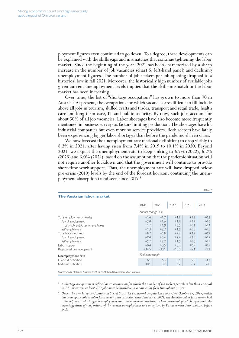
Strong economic rebound amid high uncertainty about impact of Omicron variant
124 OESTERREICHISCHE NATIONALBANK
ployment figures even continued to go down. To a degree, these developments can be explained with the skills gaps and mismatches that continue tightening the labor market. Since the beginning of the year, 2021 has been characterized by a sharp increase in the number of job vacancies (chart 5, left-hand panel) and declining unemployment figures. The number of job seekers per job opening dropped to a historical low in fall 2021. Moreover, the historically high number of available jobs given current unemployment levels implies that the skills mismatch in the labor market has been increasing.
Over time, the list of “shortage occupations” has grown to more than 70 in Austria.7 At present, the occupations for which vacancies are difficult to fill include above all jobs in tourism, skilled crafts and trades, transport and retail trade, health care and long-term care, IT and public security. By now, such jobs account for about 50% of all job vacancies. Labor shortages have also become more frequently mentioned in business surveys as factors limiting production. The shortages have hit industrial companies but even more so service providers. Both sectors have lately been experiencing bigger labor shortages than before the pandemic-driven crisis.
We now forecast the unemployment rate (national definition) to drop visibly to 8.2% in 2021, after having risen from 7.4% in 2019 to 10.1% in 2020. Beyond 2021, we expect the unemployment rate to keep sinking to 6.7% (2022), 6.2% (2023) and 6.0% (2024), based on the assumption that the pandemic situation will not require another lockdown and that the government will continue to provide short-time work support. Thus, the unemployment rate will have dropped below pre-crisis (2019) levels by the end of the forecast horizon, continuing the unem-ployment absorption trend seen since 2017.8
7 A shortage occupation is defined as an occupation for which the number of job seekers per job is less than or equal to 1.5; moreover, at least 100 jobs must be available in a particular field throughout Austria.
8 Under the new Integrated European Social Statistics Framework Regulation adopted on October 19, 2019, which has been applicable to labor force survey data collection since January 1, 2021, the Austrian labor force survey had to be adjusted, which affects employment and unemployment statistics. These methodological changes limit the meaningfulness of comparisons of the current unemployment rate as defined by Eurostat with data compiled before 2021.
Table 7
The Austrian labor market
2020 2021 2022 2023 2024
Annual change in %
Total employment (heads) –1.6 +1.7 +1.7 +1.3 +0.8Payroll employment –2.0 +1.6 +1.7 +1.4 +0.8
of which: public sector employees +1.1 +1.0 +0.5 +0.1 +0.1Self-employment +1.3 +2.7 +1.8 +0.8 +0.5
Total hours worked –8.7 +5.8 +2.3 +2.2 +0.9Payroll employment –9.4 +6.4 +2.4 +2.5 +0.9Self-employment –5.1 +2.7 +1.8 +0.8 +0.7
Labor supply –0.4 +0.5 +0.9 +0.9 +0.7Registered unemployment +14.5 –30.1 –15.0 –5.1 –1.3
Unemployment rate % of labor supply
Eurostat definition 6.1 6.3 5.4 5.0 4.7 National definition 10.1 8.2 6.7 6.2 6.0
Source: 2020: Statistics Austria; 2021 to 2024: OeNB December 2021 outlook.
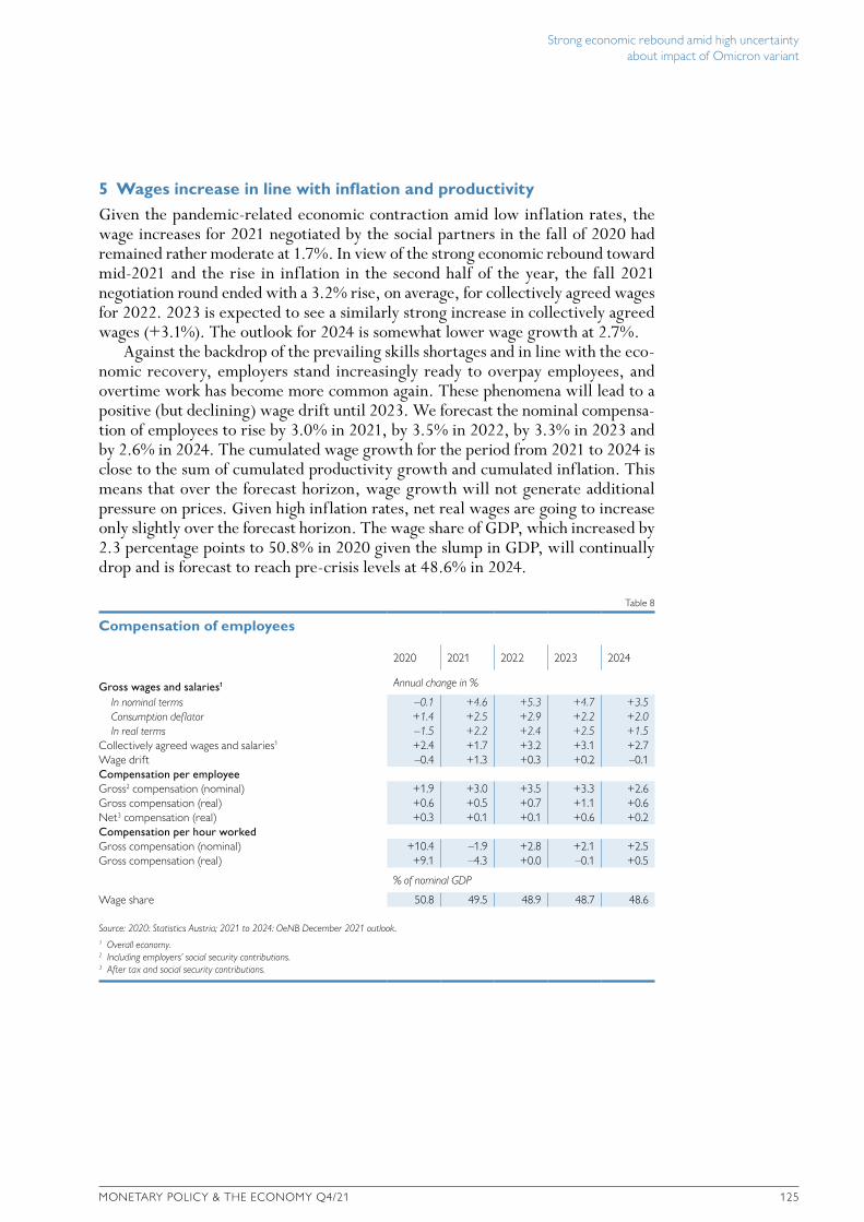
Strong economic rebound amid high uncertainty about impact of Omicron variant
MONETARY POLICY & THE ECONOMY Q4/21 125
5 Wages increase in line with inflation and productivity
Given the pandemic-related economic contraction amid low inflation rates, the wage increases for 2021 negotiated by the social partners in the fall of 2020 had remained rather moderate at 1.7%. In view of the strong economic rebound toward mid-2021 and the rise in inflation in the second half of the year, the fall 2021 negotiation round ended with a 3.2% rise, on average, for collectively agreed wages for 2022. 2023 is expected to see a similarly strong increase in collectively agreed wages (+3.1%). The outlook for 2024 is somewhat lower wage growth at 2.7%.
Against the backdrop of the prevailing skills shortages and in line with the eco-nomic recovery, employers stand increasingly ready to overpay employees, and overtime work has become more common again. These phenomena will lead to a positive (but declining) wage drift until 2023. We forecast the nominal compensa-tion of employees to rise by 3.0% in 2021, by 3.5% in 2022, by 3.3% in 2023 and by 2.6% in 2024. The cumulated wage growth for the period from 2021 to 2024 is close to the sum of cumulated productivity growth and cumulated inflation. This means that over the forecast horizon, wage growth will not generate additional pressure on prices. Given high inflation rates, net real wages are going to increase only slightly over the forecast horizon. The wage share of GDP, which increased by 2.3 percentage points to 50.8% in 2020 given the slump in GDP, will continually drop and is forecast to reach pre-crisis levels at 48.6% in 2024.
Table 8
Compensation of employees
2020 2021 2022 2023 2024
Gross wages and salaries1 Annual change in %
In nominal terms –0.1 +4.6 +5.3 +4.7 +3.5Consumption deflator +1.4 +2.5 +2.9 +2.2 +2.0In real terms –1.5 +2.2 +2.4 +2.5 +1.5
Collectively agreed wages and salaries1 +2.4 +1.7 +3.2 +3.1 +2.7Wage drift –0.4 +1.3 +0.3 +0.2 –0.1Compensation per employeeGross2 compensation (nominal) +1.9 +3.0 +3.5 +3.3 +2.6Gross compensation (real) +0.6 +0.5 +0.7 +1.1 +0.6Net3 compensation (real) +0.3 +0.1 +0.1 +0.6 +0.2Compensation per hour workedGross compensation (nominal) +10.4 –1.9 +2.8 +2.1 +2.5Gross compensation (real) +9.1 –4.3 +0.0 –0.1 +0.5
% of nominal GDP
Wage share 50.8 49.5 48.9 48.7 48.6
Source: 2020: Statistics Austria; 2021 to 2024: OeNB December 2021 outlook.1 Overall economy.2 Including employers’ social security contributions. 3 After tax and social security contributions.

Strong economic rebound amid high uncertainty about impact of Omicron variant
126 OESTERREICHISCHE NATIONALBANK
2022, will add to the rise of consumer prices for gasoline, diesel, residential heating oil and gas. Hence, we forecast annual energy inflation to level off at 10.5% in 2022, before dropping to 1.7% in 2023.
The inflation rate for nonenergy industrial goods has been rising considerably since the summer of 2021 and is set to rise to 1.8% in 2021, thus coming in well above its long-term average of 0.9%. The inflation uptick has been driven mainly by the prices for shoes and apparel, furniture and furnishings, motor vehicles as well as computers, consumer electronics and electric household appliances. Durable consumer goods in particular are likely to become more expensive as high raw material costs feed through to end user prices to some extent. Moreover, base effects and shifts in the pattern of clearance sales in 2020 led to inflation spikes in some months in 2021. Supply bottlenecks (for instance for semiconductors) and transportation chain disruptions continue to create price pressures. As the existing supply shortages are unlikely to start resolving before mid-2022 according to our assumptions, we expect the annual inflation rate for nonenergy industrial goods to rise to 1.9% in 2022.
Inflation in %; inflation contributions in percentage points
5
4
3
2
1
0
–1Jan. Mar. May July Sep. Nov.
2020Jan. Mar. May July Sep. Nov.
2021Jan. Mar. May July Sep. Nov.
2022 2023Q1 Q2 Q3 Q4
2024Q1 Q2 Q3 Q4
Contributions to Austrian HICP inflation and core inflation
Chart 4
Source: OeNB, Statistics Austria.
Food Energy Nonenergy industrial goods ServicesServices, nonenergy industrial goods HICP inflation Core inflation (excluding energy and food)
Forecast
6 Energy price-induced inflationary pressure will ease in late 2022
We project the HICP inflation rate in Austria to reach 2.7% in 2021 and rise further to 3.2% in 2022 before dropping to 2.3% in 2023 and 2% in 2024. The projections for core inflation, which excludes energy and food prices, yielded a rate of 2.3% for 2021. In 2022, we expect continued supply-side shortages together with the economic recovery to drive up core inflation somewhat further to 2.5%. Even though we assume that the supply-side shortages will largely resolve in the second half of 2022, Austria’s core inflation rate will continue to surpass its long-term average of 1.8% in 2023 (2.4%) and 2024 (2.1%).
Based on the assumption that crude oil prices will evolve in line with current crude oil futures prices, the oil price assumptions underlying this forecast, in euro terms, have been revised upward by about 20% compared with the June 2021 out-look. In recent months, we have seen not only crude oil prices rise, and hence the price of transport fuels and residential heating oil in the HICP, but also consumer prices for electricity and gas. Together with base effects from the sharp crude oil price slump in 2020, these energy price increases have been pushing up annual energy inflation to 10.9% in 2021 (2020: −5.9%). While futures prices imply that crude oil prices may recede slightly from early 2022 onward, some of the major electricity and gas suppliers have announced price increases for December 2021 and January 2022. Moreover, CO2 taxation, which is to be implemented in July
Table 9
HICP developments in Austria
2020 2021 2022 2023 2024
Annual change in %
Harmonised Index of Consumer Prices (HICP) +1.4 +2.7 +3.2 +2.3 +2.0HICP including energy –5.9 +10.9 +10.5 +1.7 +1.8HICP excluding energy +2.0 +2.3 +2.5 +2.4 +2.1
Source: 2020: Statistics Austria; 2021 to 2024: OeNB December 2021 outlook.

Strong economic rebound amid high uncertainty about impact of Omicron variant
MONETARY POLICY & THE ECONOMY Q4/21 127
2022, will add to the rise of consumer prices for gasoline, diesel, residential heating oil and gas. Hence, we forecast annual energy inflation to level off at 10.5% in 2022, before dropping to 1.7% in 2023.
The inflation rate for nonenergy industrial goods has been rising considerably since the summer of 2021 and is set to rise to 1.8% in 2021, thus coming in well above its long-term average of 0.9%. The inflation uptick has been driven mainly by the prices for shoes and apparel, furniture and furnishings, motor vehicles as well as computers, consumer electronics and electric household appliances. Durable consumer goods in particular are likely to become more expensive as high raw material costs feed through to end user prices to some extent. Moreover, base effects and shifts in the pattern of clearance sales in 2020 led to inflation spikes in some months in 2021. Supply bottlenecks (for instance for semiconductors) and transportation chain disruptions continue to create price pressures. As the existing supply shortages are unlikely to start resolving before mid-2022 according to our assumptions, we expect the annual inflation rate for nonenergy industrial goods to rise to 1.9% in 2022.
Inflation in %; inflation contributions in percentage points
5
4
3
2
1
0
–1Jan. Mar. May July Sep. Nov.
2020Jan. Mar. May July Sep. Nov.
2021Jan. Mar. May July Sep. Nov.
2022 2023Q1 Q2 Q3 Q4
2024Q1 Q2 Q3 Q4
Contributions to Austrian HICP inflation and core inflation
Chart 4
Source: OeNB, Statistics Austria.
Food Energy Nonenergy industrial goods ServicesServices, nonenergy industrial goods HICP inflation Core inflation (excluding energy and food)
Forecast

Strong economic rebound amid high uncertainty about impact of Omicron variant
128 OESTERREICHISCHE NATIONALBANK
Box 1
Energy prices skyrocket
Prices in wholesale gas and electricity markets have been rising sharply in recent months. Gas wholesale prices increased by about 350% from the start of 2021 until October, thus having
reached unprecedented levels. The under-lying price drivers were strong demand from Asia and relatively low stocks in Europe. During the same period, electricity whole-sale prices jumped by about 160%. These changes are attributable to rising cyclical demand for electricity and to rising prices for fossil fuels, such as gas, required for the production of electricity. In Austria, fossil fuels account for about one-quarter of elec-tricity production. Gas and electricity apart, crude oil prices have also continued to rise higher and higher. OPEC’s decision to expand crude oil production just somewhat did not suff ice to close the global demand-and- supply gap.
Judging from current futures prices, crude oil is the only segment in which we will see prices ease in the coming months.9 Wholesale prices for gas and electricity will remain elevated or keep rising even further; there is no evidence of futures trading at a discount before the second quarter of 2022. The pace at which wholesale prices feed through to end user prices has been accel-erating visibly since fall 2020. In general, the pass-through rate has been higher for gas prices than for electricity prices. Empir-ical data show that gas wholesale prices have been feeding through to end user prices with a lag of one month since April 2020; before that, the time lag used to be almost one year. In the case of electricity, we have lately observed a pass-through time lag of about four months, whereas wholesale and consumer electricity prices were broadly uncorrelated before the rapid acceleration of electricity prices in fall 2020. In the case of gas prices in particular, the close correlation between wholesale and end user prices may ref lect the growing market shares of smaller gas suppliers in eastern Austria.
9 Crude oil prices contracted sharply in early December 2021, after the assumptions underlying the December outlook had been defined.
EUR/MWh; Index 2015 = 100 EUR/MWh; Index 2015 = 100
Electricity prices
195
175
155
135
115
95
75
55
35
15
125
120
115
110
105
100
952017 2019 2021
Energy price developments in Austria
Chart B1
Source: OeNB, ECB, Statistics Austria.
Electricity wholesale pricesElectricity HICP (right-hand scale)
2017 2019 2021
Gas wholesale pricesGas HICP (right-hand scale)
EUR/MWh; Index 2015 = 100 EUR/MWh; Index 2015 = 100
Gas prices
100
90
80
70
60
50
40
30
20
10
0
140
130
120
110
100
90
October 2021
October 2021
2017 2019 2021
Energy price developments in Austria
Chart B1 continued
Source: OeNB, ECB, Statistics Austria.
Crude oil pricesFuel HICP (right-hand scale)
USD/barrel; Index 2015 = 100 USD/barrel; Index 2015 = 100
Oil and fuel prices
85
75
65
55
45
35
25
125
120
115
110
105
100
95
90
85
80
October 2021

Strong economic rebound amid high uncertainty about impact of Omicron variant
MONETARY POLICY & THE ECONOMY Q4/21 129
With a view to upcoming changes in gas and electricity consumer prices, energy sup-pliers have already announced sharp price increases for the coming months. In the case of electricity, these increases will be partly offset in 2022 by the announced temporary suspension of the green energy tax on con-sumers’ energy bills. At the same time, a CO2 tax10 on household energy and fuels will be payable from July 1, 2022, onward. Since household energy and transport fuels are characterized by low short-term price elastic-ities, this tax is likely to be passed through to households in full. Thus, the CO2 tax is likely to raise gas and residential heating oil prices for end users by about 8% and 14%, respec-tively, and to push up transport fuel prices for end users by between 6% and 7% (see right-hand panel). At the same time, the govern-ment’s tax reform package envisages a “climate bonus” for households, i.e. a bonus payment ranging from EUR 100 (in regions with good public transport) to EUR 200 (in regions with poor public transport).
Turning to services, we project inflation in this segment to reach 2.5% in 2021, thus remaining broadly unchanged from 2020. While rental prices have been going down during the year, hotel and other accommodation prices as well as restaurant prices went up considerably in the second half of 2021. For the time being, the renewed lockdowns in November and December 2021 and Germany’s current travel warnings for Austria are likely to slow down the acceleration of inflation in these sectors, at least temporarily. We do not expect the inflation rate for tourism- related services to start rising again until containment measures will be lifted early next year. To provide financial support to the hospitality industry, the VAT rate for food and accommodation services was cut to 5% for the period from July 2020 to December 2021. For our December 2021 outlook, we assume that the VAT rate cut will not feed through to consumer prices, in line with government intentions.
With regard to food (including alcohol and tobacco), we expect the inflation rate to reach 1.0% in 2021 and to accelerate to 2.9% in 2022. This increase is mainly attributable to rising price expectations for global agricultural commodities, which are putting pressure on imported food prices. The tobacco tax increase is expected to add another 0.2 percentage points to the inflation rate for food including tobacco in 2022. In 2023, food price inflation should drop to 2.2%, as effects on inflation brought about by the tobacco tax hike bottom out. Downward pressures on food prices will also come from a decline in global agricultural commodity prices anticipated for 2023 in line with our forecast assumptions.
10 The draft bill, which is currently in the consultation stage, provides for a levy of EUR 30 per ton of CO2 emission. Until 2025, this rate is to be raised to EUR 55.
Box 1
Energy prices skyrocket
Prices in wholesale gas and electricity markets have been rising sharply in recent months. Gas wholesale prices increased by about 350% from the start of 2021 until October, thus having
reached unprecedented levels. The under-lying price drivers were strong demand from Asia and relatively low stocks in Europe. During the same period, electricity whole-sale prices jumped by about 160%. These changes are attributable to rising cyclical demand for electricity and to rising prices for fossil fuels, such as gas, required for the production of electricity. In Austria, fossil fuels account for about one-quarter of elec-tricity production. Gas and electricity apart, crude oil prices have also continued to rise higher and higher. OPEC’s decision to expand crude oil production just somewhat did not suff ice to close the global demand-and- supply gap.
Judging from current futures prices, crude oil is the only segment in which we will see prices ease in the coming months.9 Wholesale prices for gas and electricity will remain elevated or keep rising even further; there is no evidence of futures trading at a discount before the second quarter of 2022. The pace at which wholesale prices feed through to end user prices has been accel-erating visibly since fall 2020. In general, the pass-through rate has been higher for gas prices than for electricity prices. Empir-ical data show that gas wholesale prices have been feeding through to end user prices with a lag of one month since April 2020; before that, the time lag used to be almost one year. In the case of electricity, we have lately observed a pass-through time lag of about four months, whereas wholesale and consumer electricity prices were broadly uncorrelated before the rapid acceleration of electricity prices in fall 2020. In the case of gas prices in particular, the close correlation between wholesale and end user prices may ref lect the growing market shares of smaller gas suppliers in eastern Austria.
9 Crude oil prices contracted sharply in early December 2021, after the assumptions underlying the December outlook had been defined.
EUR/MWh; Index 2015 = 100 EUR/MWh; Index 2015 = 100
Electricity prices
195
175
155
135
115
95
75
55
35
15
125
120
115
110
105
100
952017 2019 2021
Energy price developments in Austria
Chart B1
Source: OeNB, ECB, Statistics Austria.
Electricity wholesale pricesElectricity HICP (right-hand scale)
2017 2019 2021
Gas wholesale pricesGas HICP (right-hand scale)
EUR/MWh; Index 2015 = 100 EUR/MWh; Index 2015 = 100
Gas prices
100
90
80
70
60
50
40
30
20
10
0
140
130
120
110
100
90
October 2021
October 2021
2017 2019 2021
Energy price developments in Austria
Chart B1 continued
Source: OeNB, ECB, Statistics Austria.
Crude oil pricesFuel HICP (right-hand scale)
USD/barrel; Index 2015 = 100 USD/barrel; Index 2015 = 100
Oil and fuel prices
85
75
65
55
45
35
25
125
120
115
110
105
100
95
90
85
80
October 2021

Strong economic rebound amid high uncertainty about impact of Omicron variant
130 OESTERREICHISCHE NATIONALBANK
7 Budget deficit back below 3% of GDP in 2022 despite extension of COVID-19-related measures and eco-social tax reform
Thanks to the economic recovery, we see the Austrian budget deficit improving substantially in 2021 against 2020 figures. The deficit will remain elevated, however, at 5.9% of GDP. With the recovery progressing and discretionary COVID-19- related measures being discontinued, the budget deficit is expected to fall to 2.1% and thus to drop clearly below the Maastricht deficit threshold of 3% already in 2022. The eco-social tax reform, which will start to take effect in 2022, will hardly impair the positive course of Austria’s fiscal performance. On the back of high economic growth, Austria’s government debt ratio will, already in 2021, decline slightly from the historic high of 83.2% of GDP recorded in 2020. It will then decrease continuously to 75.5% of GDP in 2024.
Due to the COVID-19 pandemic, the budget balance deteriorated by about 9 percentage points to –8.3% of GDP in 2020 (pink line in chart 5). This decline was essentially driven by automatic stabilizers kicking in as the economy slowed down, which in turn considerably weakened the cyclically dependent tax revenues while driving up cyclical spending, such as unemployment payments (red bars). At the same time, the comprehensive fiscal support measures adopted in response to
the COVID-19 pandemic markedly drove up expenditure while driving down revenues through tax deferrals and tax cuts (bars in different shades of blue).
In 2021, we also expect to see a budget deficit that is very high by his-torical standards, but not as high as in 2020. Specifically, we project the budget balance to improve to –5.9% of GDP in line with the visible economic recovery and the shrinking volume of subsidies for short-time work, lost revenues and fixed costs. The significant decline in subsidies will not be reversed by the fourth nation-wide lockdown (from November 22 to December 12) and the accompanying fiscal support measures (extending the short-time work scheme, hardship funding, compensation for lost turnover and related bonus, support for nonprofit organizations and artists). These fiscal measures add up to some EUR 0.4 billion per week, judging from the costs of the full lockdowns in late 2020 and early 2021.
The cost of other expansionary fis-cal measures in the context of the COVID-19 crisis (turquoise bars) will go up slightly, however. These measures
Percentage points
1
0
–1
–2
–3
–4
–5
–6
–7
–8
–9
–102019
Change in Austria's budget balance since 2019
Chart 5
Source: OeNB.
Note: COFAG = Austrian COVID-19 funding agency.
2 Including economic stimulus packages and tax deferrals.
1 Fixed cost grants, compensation for forgone revenues, guarantees.
Short-time work (net)COFAG measures1
Eco-social tax reformOther COVID-19-related measures2
Other measuresInterest paymentsMacroeconomic effectsBudget balance
0.6
–8.3
–5.9
–2.1
–1.4–1.1
Forecast
2020 2021 2022 2023 2024
Strong economic rebound amid high uncertainty about impact of Omicron variant
MONETARY POLICY & THE ECONOMY Q4/21 131
include, above all, investment incentives for the private sector intended to stimulate economic activity, tax cuts and additional spending on medical equipment, tests and vaccination. Lower prepayments for corporate and personal income tax as well as tax deferrals will cease to play a role in 2021. Finally, the budget will be supported by windfall tax revenues, e.g. from the capital gains tax on dividends.
In the years ahead, the respective budget deficit is expected to be considerably lower. Already in 2022, Austria’s budget deficit is forecast to go back to below 3% of GDP and thus fulfill the Maastricht criterion again. This deficit improvement will be facilitated by the continued cyclical upswing and, above all, by the much smaller contribution of discretionary COVID-19-related measures. The subsidies for short-time work, compensation for lost turnover and income support for the self-employed and nonprofit organizations will have dropped to around ¼% of GDP; moreover, the temporary VAT cut for hotels and restaurants will no longer apply.
The eco-social tax reform, which will gradually take effect in 2022, will hardly impair the positive course of Austria’s fiscal performance. As many of the measures will not take effect until mid-2022 or 2023/24, the rising overall volume (green bars in chart 5) will be compensated for mainly by lower expenditure for investment incentives. Essentially, the tax reform includes carbon pricing, a bonus payment designed to compensate households for carbon pricing (“climate bonus”), the reduction of health insurance contributions for low-income earners, and lower wage tax, personal tax and corporate income tax rates (see table 10). Additional minor climate-related measures and measures to protect the environment include sub sidies for energy-efficiency renovation and for switching to greener heating systems as well as a green investment premium. Finally, the contribution from shrinking interest payments (orange bars) will continue to rise – compared with 2019 levels – at least until 2023.

Strong economic rebound amid high uncertainty about impact of Omicron variant
132 OESTERREICHISCHE NATIONALBANK
The measures to be financed from the EU’s Recovery and Resilience Fund, under the NextGenerationEU initiative, are not relevant from a fiscal perspective, as these measures will be financed via the EU and therefore do not affect national budget balances. In sum, the overall volume of these additional investment and structural measures is comparatively low, adding up to just 1% of GDP over seven years.
The rise of the debt ratio by close to 13 percentage points to 83.2% of GDP in 2020 is attributable to the contraction of the economy and the high budget deficit. Given the strong rebounding of economic activity in 2021, we forecast the debt ratio to go down slightly already in 2021 and to drop to about 75% of GDP by 2024, also on account of the declining budget deficit.
8 Risks to outlook determined by Omicron mutationThe largest downside risk to this outlook emerges from the future course and consequences of the pandemic. In this respect, the newly detected Omicron mutation of the coronavirus gives rise to a high degree of uncertainty. All we know for the time being is that the new mutation is considerably more infectious than the previous mutations. If Omicron were to lead to more frequent breakthrough infections, more severe conditions or higher rates of patients needing intensive care unit treatment, more stringent global containment measures might have to be imposed, which would have corresponding negative repercussions. Renewed shutdowns of sea port hubs crucial for world trade following renewed waves of
Table 10
Parameter changes due to eco-social tax reform
2021 2022 2023 2024 2025
EUR
CO2 price per ton of CO2 equivalent1 0 30 35 45 55Higher tax relief per child for families (up to age 18)2 1,500 2,000 2,000 2,000 2,000Higher tax relief per child for families (aged 18+)2 500 650 650 650 650Tax relief per child for single-income families/single parents2 250 450 450 450 450Taxfree employee gainsharing 0 3,000 3,000 3,000 3,000Instant asset write-off threshold 800 1,000 1,000 1,000 1,000Climate bonus per person3 0 100–200 Offsetting CO2 tax revenues
%
Personal income tax rate: income bracket EUR 18,000−31,0004 35 30 30 30 30Personal income tax rate: income bracket EUR 31,000−60,0005 42 42 40 40 40No personal income tax on the first EUR 30,000 of profit6 13 15 15 15 15Corporate income tax rate 25 25 24 23 23Reduction of employees’ health insurance contribution 3.87 Progressive reduction for low-income earners
Source: Austrian finance ministry, OeNB compilation.1 To be introduced on July 1, 2022.2 To be increased on July 1, 2022. 3 Depending on place of residence; 50% for children.4 To be lowered on July 1, 2022. 5 To be lowered on July 1, 2023.6 Applying to self-employed in the income tax scheme.

Strong economic rebound amid high uncertainty about impact of Omicron variant
MONETARY POLICY & THE ECONOMY Q4/21 133
infection would delay the clearing up of supply chain backlogs. Moreover, entry bans and travel warnings might bring global tourism to a halt once again, thus slowing down the reversal of the demand shift from goods to services, which would increase the strain on global supply chains and add to price pressures.
Another international downside risk is linked to the risk of China plunging into a real estate crisis. As residential construction investment used to be a key pillar of the Chinese economy, an insolvency crisis in the real estate sector might have a knock-on effect on other sectors of the economy and on other Asian countries. Furthermore, shutting down further power stations with a view to meeting China’s emissions goals might dampen output, with short-term growth goals competing with longer-term climate goals. If the Chinese economy were to grow at a lower rate, the international framework conditions on which this forecast is based would be worse than assumed, which would have an adverse impact on exports.
By contrast, we consider a faster availability of COVID-19 vaccines in emerging economies as the key upside risk to our outlook. Furthermore, the global supply bottlenecks might ease earlier than expected (i.e. before the summer of 2022), which would improve the growth outlook for production, goods exports and investment.
The domestic risks to this outlook are also mostly related to the pandemic. A renewed spike of infections might lead to further movement restrictions in the winter of 2021/22, which would mainly affect tourism as well as the retail sector and high-contact services. Apart from this downside risk, we also see upside risks to Austrian growth, above all in 2022. The rebound after the fourth lockdown, for instance, might be stronger than expected. There is also a chance that the unwinding of excess savings accumulated during the pandemic might be accelerated, which would contribute to a faster rebound.
With regard to inflation, the risks to this outlook are predominantly to the upside across the forecast horizon. For 2022, upside risks may arise from a potential pass-through of discontinued VAT cuts to consumer prices for accommodation and restaurant services. Likewise, the inflation rate for nonenergy industrial goods might run higher than projected if the dynamic growth of industrial producer prices were to continue. In the medium run, additional measures needed to secure the achievement of emissions goals (CO2 neutrality) might drive further energy price increases, in particular for oil and gas. Higher inflation expectations and labor shortages (in some sectors) might support wage growth and create additional price pressure.
9 Past outlook revisions driven by stronger growth around mid-2021The upward revision of Austrian GDP growth, compared with the June 2021 out-look, to 4.9% was mainly driven by the unexpected strength of the economy in mid-2021. The upward revision was offsetting the impact of the downward revi-sion of GDP growth until the first quarter of 2021 and the fourth wave of the pan-demic, causing output growth to be 1.0 percentage point higher than expected in the June 2021 outlook. The outlook for 2022 was, ultimately, subject to just a slight upward revision (+0.1 percentage point). The higher statistical overhang from 2021 and a positive effect from external assumptions given the easing of

Strong economic rebound amid high uncertainty about impact of Omicron variant
134 OESTERREICHISCHE NATIONALBANK
global supply bottlenecks11 would have called for a substantial upward revision. These positive effects were, however, compensated by the negative effects of the fourth wave of COVID-19 infections. Furthermore, we expect easing supply bottlenecks to contribute 1.2 percentage points to GDP growth in 2023. However, given stronger growth in 2021 and 2022, the economic catching-up process will have progressed further by the start of 2023 than expected in the June 2021 outlook. To take this frontloading effect into account, we therefore added an offsetting impact of 0.5 percentage points.
Finally, the inflation rate has been subject to a significant upward revision for the entire forecast horizon, but above all for 2022, compared with the June 2021 outlook. The upward revisions were 0.7 percentage points for 2021, about 1.4 per-centage points for 2022 and 0.5 percentage points for 2023. The revisions for 2021 and 2022 were above all driven by rising crude oil prices. Other factors include higher-than-expected price increases for gas and electricity, the introduction of CO2 taxation and persistent supply-side bottlenecks.
11 The supply bottlenecks were considerably stronger and more persistent than expected in June. Therefore, the impact from the easing of the relevant shortages will materialize at a later point and will also be stronger than initially expected.
Table 11
Breakdown of revisions to the outlook
GDP HICP
2021 2022 2023 2021 2022 2023
Annual change in %
December 2021 outlook +4.9 +4.3 +2.6 +2.7 +3.2 +2.3June 2021 outlook +3.9 +4.2 +1.9 +2.0 +1.8 +1.8Difference +1.0 +0.1 +0.7 +0.7 +1.4 +0.5
Caused by: Percentage points
External assumptions –0.2 +0.3 +1.2 +0.1 +0.7 +0.2New data1 +1.6 +1.2 +0.0 +0.6 +0.4 +0.1of which: revisions to historical data up to Q1 21 –0.6 +0.0 +0.0 +0.0 +0.0 +0.0
projection errors for Q2 21 and Q3 21 +2.3 +1.2 +0.0 +0.6 +0.4 +0.1Other reasons2 –0.5 –1.4 –0.5 +0.0 +0.3 +0.2
Source: OeNB June 2021 and December 2021 outlooks.
Note: The sum of growth contributions subject to individual revisions may differ from the overall revision due to rounding.1 “New data” refer to data on GDP and/or inflation that have become available since the publication of the preceding OeNB outlook.2 Different assumptions about trends in domestic variables such as wages, government consumption, effects of tax measures, other changes in
assessments and model changes.
Table 12
December 2021 outlook and revisions since the June 2021 outlook
December 2021 Revisions to June 2021 outlook
2021 2022 2023 2024 2021 2022 2023
Economic activity Annual change in % (real)
Gross domestic product (GDP) +4.9 +4.3 +2.6 +1.8 1.0 0.1 0.7 Private consumption +1.8 +5.7 +3.4 +2.4 –2.2 –0.1 1.6 Government consumption +5.3 –0.9 +0.3 +0.7 3.2 –1.4 –0.5 Gross fixed capital formation +5.7 +2.7 +1.9 +1.3 1.0 –0.6 0.1 Exports of goods and services +10.5 +3.2 +4.8 +2.5 3.4 –3.2 1.4 Imports of goods and services +11.3 +1.9 +4.5 +2.4 3.9 –4.4 1.5
Current account balance –1.3 –0.5 +1.0 +1.3 –3.4 –2.7 –1.4
Import-adjusted contributions to real GDP growth1 Percentage points
Private consumption +0.6 +2.0 +1.2 +0.8 –1.1 0.3 0.5 Government consumption +0.9 –0.2 +0.0 +0.1 0.5 –0.2 –0.1 Gross fixed capital formation +0.8 +0.4 +0.3 +0.2 –0.1 0.2 0.0 Domestic demand (excluding changes in inventories) +2.3 +2.2 +1.5 +1.2 –0.6 0.2 0.4 Exports +2.9 +0.9 +1.4 +0.8 0.4 –0.3 0.3 Changes in inventories (including statistical discrepancy) +0.9 +0.0 +0.0 +0.0 1.0 0.0 0.0
Prices Annual change in %
Harmonised Index of Consumer Prices (HICP) +2.7 +3.2 +2.3 +2.0 0.7 1.4 0.5 Private consumption expenditure deflator +2.5 +2.9 +2.2 +2.0 0.4 1.1 0.5 GDP deflator +2.3 +2.3 +2.5 +1.9 0.0 0.4 0.9 Unit labor costs (whole economy) –0.2 +0.9 +2.0 +1.6 0.4 0.8 0.6 Compensation per employee (nominal) +3.0 +3.5 +3.3 +2.6 0.8 0.6 0.7 Compensation per hour worked (nominal) –1.9 +2.8 +2.1 +2.5 –0.5 2.5 0.3 Import prices +4.9 +3.9 +1.8 +1.9 3.3 2.0 –0.1 Export prices +2.6 +2.8 +2.3 +1.8 0.9 0.8 0.8 Terms of trade –2.2 –1.1 +0.4 –0.1 –2.3 –1.2 0.7
Income and savingsReal disposable household income –2.8 +3.3 +3.6 +2.5 –3.4 0.9 2.2
% of nominal disposable household income
Saving ratio +9.6 +7.1 +7.3 +7.4 –1.4 –1.0 –0.5
Labor market Annual change in %
Payroll employment +1.6 +1.7 +1.4 +0.8 0.4 0.1 0.5 Hours worked (payroll employment) +6.4 +2.4 +2.5 +0.9 1.7 –1.7 0.8
% of labor supply
Unemployment rate (Eurostat definition) 6.3 5.4 5.0 4.7 1.1 0.6 0.4
Public finances % of nominal GDP
Budget balance (Maastricht definition) –5.9 –2.1 –1.4 –1.1 1.0 0.7 0.6 Government debt 82.7 79.5 77.0 75.5 –2.4 –3.3 –4.9
Source: 2020 (actual f igures): WIFO, Statistics Austria, OeNB; OeNB June 2021 and December 2021 outlooks.1 The import-adjusted growth contributions were calculated by offsetting each final demand component with the corresponding imports, which were obtained from input-output tables.

Strong economic rebound amid high uncertainty about impact of Omicron variant
MONETARY POLICY & THE ECONOMY Q4/21 135
global supply bottlenecks11 would have called for a substantial upward revision. These positive effects were, however, compensated by the negative effects of the fourth wave of COVID-19 infections. Furthermore, we expect easing supply bottlenecks to contribute 1.2 percentage points to GDP growth in 2023. However, given stronger growth in 2021 and 2022, the economic catching-up process will have progressed further by the start of 2023 than expected in the June 2021 outlook. To take this frontloading effect into account, we therefore added an offsetting impact of 0.5 percentage points.
Finally, the inflation rate has been subject to a significant upward revision for the entire forecast horizon, but above all for 2022, compared with the June 2021 outlook. The upward revisions were 0.7 percentage points for 2021, about 1.4 per-centage points for 2022 and 0.5 percentage points for 2023. The revisions for 2021 and 2022 were above all driven by rising crude oil prices. Other factors include higher-than-expected price increases for gas and electricity, the introduction of CO2 taxation and persistent supply-side bottlenecks.
11 The supply bottlenecks were considerably stronger and more persistent than expected in June. Therefore, the impact from the easing of the relevant shortages will materialize at a later point and will also be stronger than initially expected.
Table 11
Breakdown of revisions to the outlook
GDP HICP
2021 2022 2023 2021 2022 2023
Annual change in %
December 2021 outlook +4.9 +4.3 +2.6 +2.7 +3.2 +2.3June 2021 outlook +3.9 +4.2 +1.9 +2.0 +1.8 +1.8Difference +1.0 +0.1 +0.7 +0.7 +1.4 +0.5
Caused by: Percentage points
External assumptions –0.2 +0.3 +1.2 +0.1 +0.7 +0.2New data1 +1.6 +1.2 +0.0 +0.6 +0.4 +0.1of which: revisions to historical data up to Q1 21 –0.6 +0.0 +0.0 +0.0 +0.0 +0.0
projection errors for Q2 21 and Q3 21 +2.3 +1.2 +0.0 +0.6 +0.4 +0.1Other reasons2 –0.5 –1.4 –0.5 +0.0 +0.3 +0.2
Source: OeNB June 2021 and December 2021 outlooks.
Note: The sum of growth contributions subject to individual revisions may differ from the overall revision due to rounding.1 “New data” refer to data on GDP and/or inflation that have become available since the publication of the preceding OeNB outlook.2 Different assumptions about trends in domestic variables such as wages, government consumption, effects of tax measures, other changes in
assessments and model changes.
Table 12
December 2021 outlook and revisions since the June 2021 outlook
December 2021 Revisions to June 2021 outlook
2021 2022 2023 2024 2021 2022 2023
Economic activity Annual change in % (real)
Gross domestic product (GDP) +4.9 +4.3 +2.6 +1.8 1.0 0.1 0.7 Private consumption +1.8 +5.7 +3.4 +2.4 –2.2 –0.1 1.6 Government consumption +5.3 –0.9 +0.3 +0.7 3.2 –1.4 –0.5 Gross fixed capital formation +5.7 +2.7 +1.9 +1.3 1.0 –0.6 0.1 Exports of goods and services +10.5 +3.2 +4.8 +2.5 3.4 –3.2 1.4 Imports of goods and services +11.3 +1.9 +4.5 +2.4 3.9 –4.4 1.5
Current account balance –1.3 –0.5 +1.0 +1.3 –3.4 –2.7 –1.4
Import-adjusted contributions to real GDP growth1 Percentage points
Private consumption +0.6 +2.0 +1.2 +0.8 –1.1 0.3 0.5 Government consumption +0.9 –0.2 +0.0 +0.1 0.5 –0.2 –0.1 Gross fixed capital formation +0.8 +0.4 +0.3 +0.2 –0.1 0.2 0.0 Domestic demand (excluding changes in inventories) +2.3 +2.2 +1.5 +1.2 –0.6 0.2 0.4 Exports +2.9 +0.9 +1.4 +0.8 0.4 –0.3 0.3 Changes in inventories (including statistical discrepancy) +0.9 +0.0 +0.0 +0.0 1.0 0.0 0.0
Prices Annual change in %
Harmonised Index of Consumer Prices (HICP) +2.7 +3.2 +2.3 +2.0 0.7 1.4 0.5 Private consumption expenditure deflator +2.5 +2.9 +2.2 +2.0 0.4 1.1 0.5 GDP deflator +2.3 +2.3 +2.5 +1.9 0.0 0.4 0.9 Unit labor costs (whole economy) –0.2 +0.9 +2.0 +1.6 0.4 0.8 0.6 Compensation per employee (nominal) +3.0 +3.5 +3.3 +2.6 0.8 0.6 0.7 Compensation per hour worked (nominal) –1.9 +2.8 +2.1 +2.5 –0.5 2.5 0.3 Import prices +4.9 +3.9 +1.8 +1.9 3.3 2.0 –0.1 Export prices +2.6 +2.8 +2.3 +1.8 0.9 0.8 0.8 Terms of trade –2.2 –1.1 +0.4 –0.1 –2.3 –1.2 0.7
Income and savingsReal disposable household income –2.8 +3.3 +3.6 +2.5 –3.4 0.9 2.2
% of nominal disposable household income
Saving ratio +9.6 +7.1 +7.3 +7.4 –1.4 –1.0 –0.5
Labor market Annual change in %
Payroll employment +1.6 +1.7 +1.4 +0.8 0.4 0.1 0.5 Hours worked (payroll employment) +6.4 +2.4 +2.5 +0.9 1.7 –1.7 0.8
% of labor supply
Unemployment rate (Eurostat definition) 6.3 5.4 5.0 4.7 1.1 0.6 0.4
Public finances % of nominal GDP
Budget balance (Maastricht definition) –5.9 –2.1 –1.4 –1.1 1.0 0.7 0.6 Government debt 82.7 79.5 77.0 75.5 –2.4 –3.3 –4.9
Source: 2020 (actual f igures): WIFO, Statistics Austria, OeNB; OeNB June 2021 and December 2021 outlooks.1 The import-adjusted growth contributions were calculated by offsetting each final demand component with the corresponding imports, which were obtained from input-output tables.

Strong economic rebound amid high uncertainty about impact of Omicron variant
136 OESTERREICHISCHE NATIONALBANK
Annex of tables: detailed results
Table 13
Demand components (real)
Chained volume data (reference year = 2015)
2020 2021 2022 2023 2024 2020 2021 2022 2023 2024
EUR million Annual change in %
Private consumption 175,110 178,289 188,475 194,880 199,481 –8.4 +1.8 +5.7 +3.4 +2.4Government consumption 71,467 75,236 74,536 74,750 75,242 –0.4 +5.3 –0.9 +0.3 +0.7Gross fixed capital formation 88,278 93,320 95,808 97,666 98,945 –5.0 +5.7 +2.7 +1.9 +1.3of which: investment in plant and
equipment 28,502 31,064 31,847 32,384 32,893 –8.3 +9.0 +2.5 +1.7 +1.6residential construction investment 17,212 17,705 17,631 17,962 18,233 +1.8 +2.9 –0.4 +1.9 +1.5nonresidential construction investment and other investment 22,681 23,975 25,588 26,114 26,324 –7.0 +5.7 +6.7 +2.1 +0.8
Changes in inventories (including statistical discrepancy) 3,254 8,839 9,802 9,941 9,951 x x x x xDomestic demand 338,109 355,684 368,621 377,237 383,618 –5.4 +5.2 +3.6 +2.3 +1.7
Exports of goods and services 190,465 210,544 217,191 227,717 233,425 –11.5 +10.5 +3.2 +4.8 +2.5Imports of goods and services 180,545 200,993 204,877 214,053 219,161 –9.3 +11.3 +1.9 +4.5 +2.4Net exports 9,920 9,551 12,313 13,664 14,264 x x x x x
Gross domestic product 348,029 365,235 380,935 390,901 397,882 –6.8 +4.9 +4.3 +2.6 +1.8
Source: 2020: Statistics Austria; 2021 to 2024: OeNB December 2021 outlook.
Table 14
Demand components (nominal)
2020 2021 2022 2023 2024 2020 2021 2022 2023 2024
EUR million Annual change in %
Private consumption 190,212 198,450 215,738 228,080 238,105 –7.2 +4.3 +8.7 +5.7 +4.4Government consumption 80,318 86,117 87,034 89,673 92,215 +3.9 +7.2 +1.1 +3.0 +2.8Gross fixed capital formation 95,818 104,371 110,149 115,150 119,413 –3.3 +8.9 +5.5 +4.5 +3.7Changes in inventories (including statistical discrepancy) 2,412 12,455 15,083 15,240 14,788 x x x x xDomestic demand 368,759 401,393 428,005 448,143 464,521 –3.7 +8.8 +6.6 +4.7 +3.7
Exports of goods and services 193,997 220,099 233,394 250,297 261,197 –12.2 +13.5 +6.0 +7.2 +4.4Imports of goods and services 184,153 214,902 227,621 242,197 252,581 –10.9 +16.7 +5.9 +6.4 +4.3Net exports 9,844 5,197 5,773 8,100 8,616 x x x x x
Gross domestic product 378,603 406,590 433,778 456,242 473,137 –4.7 +7.4 +6.7 +5.2 +3.7
Source: 2020: Statistics Austria; 2021 to 2024: OeNB December 2021 outlook.
Table 15
Demand components (deflators)
2020 2021 2022 2023 2024 2020 2021 2022 2023 2024
2010 = 100 Annual change in %
Private consumption 108.6 111.3 114.5 117.0 119.4 +1.4 +2.5 +2.9 +2.2 +2.0Government consumption 112.4 114.5 116.8 120.0 122.6 +4.3 +1.8 +2.0 +2.7 +2.2Gross fixed capital formation 108.5 111.8 115.0 117.9 120.7 +1.8 +3.1 +2.8 +2.6 +2.4Domestic demand (excluding changes in inventories) 109.4 112.1 115.1 117.9 120.4 +2.1 +2.5 +2.6 +2.4 +2.1
Exports of goods and services 101.9 104.5 107.4 109.9 111.9 –0.8 +2.6 +2.8 +2.3 +1.8Imports of goods and services 101.9 106.9 111.1 113.1 115.2 –1.8 +4.9 +3.9 +1.8 +1.9Terms of trade 99.9 97.7 96.7 97.1 97.1 +1.0 –2.2 –1.1 +0.4 –0.1
Gross domestic product 108.8 111.3 113.9 116.7 118.9 +2.3 +2.3 +2.3 +2.5 +1.9
Source: 2020: Statistics Austria; 2021 to 2024: OeNB December 2021 outlook.
Table 16
Labor market
2020 2021 2022 2023 2024 2020 2021 2022 2023 2024
Thousands Annual change in %
Total employment 4,466.0 4,542.8 4,621.7 4,681.2 4,718 –1.6 +1.7 +1.7 +1.3 +0.8of which: private sector 3,700.0 3,769.1 3,844.1 3,902.7 3,939 –2.1 +1.9 +2.0 +1.5 +0.9
Payroll employment (national accounts definition) 3,918.8 3,980.8 4,049.4 4,104.2 4,138 –2.0 +1.6 +1.7 +1.4 +0.8
% of labor supply
Unemployment rate (Eurostat definition) 6.1 6.3 5.4 5.0 4.7 x x x x x
EUR per real unit of output x 100
Unit labor costs (whole economy)1 63.1 63.0 63.5 64.8 65.8 +7.7 –0.2 +0.9 +2.0 +1.6
EUR thousand per employee
Labor productivity (whole economy)2 77.9 80.4 82.4 83.5 84.3 –5.4 +3.2 +2.5 +1.3 +1.0
EUR thousand
Compensation per employee (real)3 45.2 45.5 45.8 46.2 46.5 +0.5 +0.5 +0.6 +1.0 +0.6
EUR thousand (nominal)
Compensation per employee (gross) 49.1 50.6 52.4 54.1 55.5 +1.9 +3.0 +3.5 +3.3 +2.6
EUR million (nominal)
Total compensation of employees (gross) 192,519 201,420 212,074 222,052 229,759 –0.1 +4.6 +5.3 +4.7 +3.5
Source: 2020: Statistics Austria; 2021 to 2024: OeNB December 2021 outlook.1 Gross wages and salaries divided by real GDP.2 Real GDP divided by total employment.3 Gross wages and salaries per employee divided by private consumption expenditure deflator.

Strong economic rebound amid high uncertainty about impact of Omicron variant
MONETARY POLICY & THE ECONOMY Q4/21 137
Annex of tables: detailed results
Table 13
Demand components (real)
Chained volume data (reference year = 2015)
2020 2021 2022 2023 2024 2020 2021 2022 2023 2024
EUR million Annual change in %
Private consumption 175,110 178,289 188,475 194,880 199,481 –8.4 +1.8 +5.7 +3.4 +2.4Government consumption 71,467 75,236 74,536 74,750 75,242 –0.4 +5.3 –0.9 +0.3 +0.7Gross fixed capital formation 88,278 93,320 95,808 97,666 98,945 –5.0 +5.7 +2.7 +1.9 +1.3of which: investment in plant and
equipment 28,502 31,064 31,847 32,384 32,893 –8.3 +9.0 +2.5 +1.7 +1.6residential construction investment 17,212 17,705 17,631 17,962 18,233 +1.8 +2.9 –0.4 +1.9 +1.5nonresidential construction investment and other investment 22,681 23,975 25,588 26,114 26,324 –7.0 +5.7 +6.7 +2.1 +0.8
Changes in inventories (including statistical discrepancy) 3,254 8,839 9,802 9,941 9,951 x x x x xDomestic demand 338,109 355,684 368,621 377,237 383,618 –5.4 +5.2 +3.6 +2.3 +1.7
Exports of goods and services 190,465 210,544 217,191 227,717 233,425 –11.5 +10.5 +3.2 +4.8 +2.5Imports of goods and services 180,545 200,993 204,877 214,053 219,161 –9.3 +11.3 +1.9 +4.5 +2.4Net exports 9,920 9,551 12,313 13,664 14,264 x x x x x
Gross domestic product 348,029 365,235 380,935 390,901 397,882 –6.8 +4.9 +4.3 +2.6 +1.8
Source: 2020: Statistics Austria; 2021 to 2024: OeNB December 2021 outlook.
Table 14
Demand components (nominal)
2020 2021 2022 2023 2024 2020 2021 2022 2023 2024
EUR million Annual change in %
Private consumption 190,212 198,450 215,738 228,080 238,105 –7.2 +4.3 +8.7 +5.7 +4.4Government consumption 80,318 86,117 87,034 89,673 92,215 +3.9 +7.2 +1.1 +3.0 +2.8Gross fixed capital formation 95,818 104,371 110,149 115,150 119,413 –3.3 +8.9 +5.5 +4.5 +3.7Changes in inventories (including statistical discrepancy) 2,412 12,455 15,083 15,240 14,788 x x x x xDomestic demand 368,759 401,393 428,005 448,143 464,521 –3.7 +8.8 +6.6 +4.7 +3.7
Exports of goods and services 193,997 220,099 233,394 250,297 261,197 –12.2 +13.5 +6.0 +7.2 +4.4Imports of goods and services 184,153 214,902 227,621 242,197 252,581 –10.9 +16.7 +5.9 +6.4 +4.3Net exports 9,844 5,197 5,773 8,100 8,616 x x x x x
Gross domestic product 378,603 406,590 433,778 456,242 473,137 –4.7 +7.4 +6.7 +5.2 +3.7
Source: 2020: Statistics Austria; 2021 to 2024: OeNB December 2021 outlook.
Table 15
Demand components (deflators)
2020 2021 2022 2023 2024 2020 2021 2022 2023 2024
2010 = 100 Annual change in %
Private consumption 108.6 111.3 114.5 117.0 119.4 +1.4 +2.5 +2.9 +2.2 +2.0Government consumption 112.4 114.5 116.8 120.0 122.6 +4.3 +1.8 +2.0 +2.7 +2.2Gross fixed capital formation 108.5 111.8 115.0 117.9 120.7 +1.8 +3.1 +2.8 +2.6 +2.4Domestic demand (excluding changes in inventories) 109.4 112.1 115.1 117.9 120.4 +2.1 +2.5 +2.6 +2.4 +2.1
Exports of goods and services 101.9 104.5 107.4 109.9 111.9 –0.8 +2.6 +2.8 +2.3 +1.8Imports of goods and services 101.9 106.9 111.1 113.1 115.2 –1.8 +4.9 +3.9 +1.8 +1.9Terms of trade 99.9 97.7 96.7 97.1 97.1 +1.0 –2.2 –1.1 +0.4 –0.1
Gross domestic product 108.8 111.3 113.9 116.7 118.9 +2.3 +2.3 +2.3 +2.5 +1.9
Source: 2020: Statistics Austria; 2021 to 2024: OeNB December 2021 outlook.
Table 16
Labor market
2020 2021 2022 2023 2024 2020 2021 2022 2023 2024
Thousands Annual change in %
Total employment 4,466.0 4,542.8 4,621.7 4,681.2 4,718 –1.6 +1.7 +1.7 +1.3 +0.8of which: private sector 3,700.0 3,769.1 3,844.1 3,902.7 3,939 –2.1 +1.9 +2.0 +1.5 +0.9
Payroll employment (national accounts definition) 3,918.8 3,980.8 4,049.4 4,104.2 4,138 –2.0 +1.6 +1.7 +1.4 +0.8
% of labor supply
Unemployment rate (Eurostat definition) 6.1 6.3 5.4 5.0 4.7 x x x x x
EUR per real unit of output x 100
Unit labor costs (whole economy)1 63.1 63.0 63.5 64.8 65.8 +7.7 –0.2 +0.9 +2.0 +1.6
EUR thousand per employee
Labor productivity (whole economy)2 77.9 80.4 82.4 83.5 84.3 –5.4 +3.2 +2.5 +1.3 +1.0
EUR thousand
Compensation per employee (real)3 45.2 45.5 45.8 46.2 46.5 +0.5 +0.5 +0.6 +1.0 +0.6
EUR thousand (nominal)
Compensation per employee (gross) 49.1 50.6 52.4 54.1 55.5 +1.9 +3.0 +3.5 +3.3 +2.6
EUR million (nominal)
Total compensation of employees (gross) 192,519 201,420 212,074 222,052 229,759 –0.1 +4.6 +5.3 +4.7 +3.5
Source: 2020: Statistics Austria; 2021 to 2024: OeNB December 2021 outlook.1 Gross wages and salaries divided by real GDP.2 Real GDP divided by total employment.3 Gross wages and salaries per employee divided by private consumption expenditure deflator.

Strong economic rebound amid high uncertainty about impact of Omicron variant
138 OESTERREICHISCHE NATIONALBANK
Table 17
Current account balance
2020 2021 2022 2023 2024 2020 2021 2022 2023 2024
EUR million % of nominal GDP
Balance of trade 10,899.0 1,361.2 5,241.0 11,221.4 13,839.0 2.9 0.3 1.2 2.5 2.9Balance of goods 3,032.0 –247.2 –1,190.9 454.2 1,994.8 0.8 –0.1 –0.3 0.1 0.4Balance of services 7,867.0 1,608.4 6,431.9 10,767.2 11,844.0 2.1 0.4 1.5 2.4 2.5
Balance of primary income –426.0 –3,480.0 –4,072.0 –3,696.6 –3,718.3 –0.1 –0.9 –0.9 –0.8 –0.8 Balance of secondary income –3,271.0 –3,330.1 –3,340.3 –3,080.8 –3,745.6 –0.9 –0.8 –0.8 –0.7 –0.8 Current account balance 7,202.0 –5,448.9 –2,171.3 4,444.0 6,374.6 1.9 –1.3 –0.5 1.0 1.3
Source: 2020: Statistics Austria; 2021 to 2024: OeNB December 2021 outlook.
Table 18
Quarterly outlook results
2021 2022 2023 2024 2021 2022 2023 2024
Q1 Q2 Q3 Q4 Q1 Q2 Q3 Q4 Q1 Q2 Q3 Q4 Q1 Q2 Q3 Q4
Prices, wages, costs Annual change in %
HICP +2.7 +3.2 +2.3 +2.0 +1.5 +2.6 +3.1 +3.8 +3.9 +3.5 +3.2 +2.3 +2.5 +2.4 +2.2 +2.0 +2.0 +2.0 +2.1 +2.0HICP excluding energy +2.3 +2.5 +2.4 +2.1 +1.8 +2.2 +2.4 +2.6 +2.6 +2.6 +2.4 +2.4 +2.5 +2.3 +2.5 +2.1 +2.0 +2.0 +2.3 +2.2Private consumption expenditure deflator +2.5 +2.9 +2.2 +2.0 +1.5 +2.4 +2.3 +3.6 +3.2 +3.1 +3.0 +2.2 +2.3 +2.3 +2.2 +2.1 +1.9 +1.9 +2.0 +2.1Gross fixed capital formation deflator +3.1 +2.8 +2.6 +2.4 +1.6 +3.2 +4.0 +3.3 +3.6 +2.6 +2.0 +3.0 +2.7 +2.6 +2.5 +2.4 +2.4 +2.4 +2.4 +2.3GDP deflator +2.3 +2.3 +2.5 +1.9 +2.0 +0.9 +2.1 +4.2 +3.1 +3.1 +2.4 +0.7 +2.2 +2.4 +2.7 +2.6 +2.2 +2.0 +1.7 +1.7Unit labor costs –0.2 +0.9 +2.0 +1.6 +3.8 –2.6 +0.7 –2.6 –1.2 +0.1 +2.3 +2.6 +2.1 +2.0 +1.7 +2.1 +2.2 +2.0 +1.5 +0.7Compensation per employee (nominal) +3.0 +3.5 +3.3 +2.6 +1.4 +5.4 +3.6 +1.7 +3.1 +3.4 +3.2 +4.3 +3.9 +3.1 +3.0 +3.3 +3.3 +3.1 +2.5 +1.6Productivity +3.2 +2.5 +1.3 +1.0 –2.3 +8.2 +2.9 +4.4 +4.4 +3.3 +0.9 +1.6 +1.7 +1.1 +1.2 +1.2 +1.1 +1.0 +1.0 +0.9Compensation per employee (real) +0.5 +0.6 +1.0 +0.6 –0.1 +3.0 +1.2 –1.8 –0.1 +0.3 +0.2 +2.1 +1.5 +0.8 +0.7 +1.2 +1.4 +1.1 +0.5 –0.5 Import deflator +4.9 +3.9 +1.8 +1.9 +1.2 +5.6 +6.3 +6.6 +5.6 +4.5 +3.2 +2.4 +1.8 +1.8 +1.9 +1.9 +2.0 +1.9 +1.8 +1.7Export deflator +2.6 +2.8 +2.3 +1.8 +0.9 +2.2 +3.2 +4.1 +3.5 +2.9 +2.5 +2.4 +2.4 +2.4 +2.3 +2.1 +1.9 +1.8 +1.8 +1.7Terms of trade –2.2 –1.1 +0.4 –0.1 –0.3 –3.2 –2.9 –2.3 –2.0 –1.5 –0.7 +0.0 +0.6 +0.6 +0.4 +0.1 +0.0 –0.1 –0.1 +0.0
Economic activity Annual or quarterly changes in % (real)
GDP +4.9 +4.3 +2.6 +1.8 –0.4 +4.2 +3.8 –1.2 +0.8 +1.3 +0.6 +0.6 +0.6 +0.6 +0.5 +0.5 +0.4 +0.4 +0.4 +0.4Private consumption +1.8 +5.7 +3.4 +2.4 –3.5 +4.0 +7.0 –4.5 +3.8 +0.7 +0.5 +1.3 +0.9 +0.8 +0.7 +0.7 +0.6 +0.5 +0.4 +0.3Government consumption +5.3 –0.9 +0.3 +0.7 +0.5 +1.7 +0.5 –0.6 –0.9 –0.4 –0.1 +0.1 +0.3 +0.1 +0.0 +0.0 +0.1 +0.3 +0.3 +0.4Gross fixed capital formation +5.7 +2.7 +1.9 +1.3 +4.7 +0.8 –2.8 +1.9 +1.8 +0.5 +0.5 +0.4 +0.6 +0.5 +0.4 +0.4 +0.5 +0.2 +0.1 +0.1Exports +10.5 +3.2 +4.8 +2.5 –1.6 +13.5 –2.3 –1.7 –1.5 +3.6 +2.0 +1.2 +0.8 +0.8 +0.8 +0.7 +0.5 +0.6 +0.6 +0.6Imports +11.3 +1.9 +4.5 +2.4 +5.9 +3.4 –2.1 –2.6 +1.1 +2.6 +1.6 +1.5 +0.8 +0.7 +0.7 +0.7 +0.6 +0.5 +0.5 +0.5
Contribution to real GDP growth in percentage points
Domestic demand +3.4 +3.3 +2.2 +1.6 –0.4 +2.5 +2.8 –1.9 +2.1 +0.4 +0.3 +0.8 +0.6 +0.5 +0.5 +0.5 +0.4 +0.4 +0.3 +0.3Net exports –0.1 +0.8 +0.4 +0.2 –4.1 +5.6 –0.2 +0.4 –1.4 +0.6 +0.3 –0.1 +0.0 +0.1 +0.0 +0.0 +0.0 +0.1 +0.1 +0.1Changes in inventories +1.6 +0.3 +0.0 +0.0 +4.2 –3.9 +1.2 +0.3 +0.1 +0.3 +0.0 +0.0 +0.0 +0.0 +0.0 +0.0 +0.0 +0.0 +0.0 +0.0
Labor market % of labor supply
Unemployment rate (Eurostat definition) 6.3 5.4 5.0 4.7 7.0 6.7 5.7 5.6 5.8 5.4 5.3 5.2 5.1 5.0 5.0 4.9 4.8 4.8 4.7 4.7
Annual or quarterly changes in %
Total employment +1.7 +1.7 +1.3 +0.8 –0.7 +2.1 +1.4 –0.8 +0.5 +0.4 +0.5 +0.3 +0.2 +0.3 +0.3 +0.2 +0.1 +0.2 +0.2 +0.2of which: private sector +1.9 +2.0 +1.5 +0.9 –0.8 +2.5 +1.6 –1.0 +0.6 +0.5 +0.6 +0.4 +0.3 +0.4 +0.3 +0.3 +0.1 +0.2 +0.2 +0.3
Payroll employment +1.6 +1.7 +1.4 +0.8 –0.9 +2.2 +1.3 –0.9 +0.5 +0.5 +0.6 +0.3 +0.2 +0.3 +0.3 +0.2 +0.1 +0.2 +0.2 +0.2
Additional variables Annual or quarterly changes in % (real)
Disposable household income –2.8 +3.3 +3.6 +2.5 –10.6 +2.4 +3.6 –2.1 +1.0 +1.0 +1.0 +0.9 +0.8 +0.8 +1.0 +1.1 +0.8 +0.3 +0.1 –0.3
% of real GDP
Output gap –3.2 –0.8 +0.1 +0.3 –7.0 –3.6 –0.3 –2.0 –1.7 –0.8 –0.6 –0.4 –0.1 +0.1 +0.2 +0.3 +0.3 +0.3 +0.3 +0.2
Source: OeNB December 2021 outlook.
Note: Quarterly values based on seasonally and working day-adjusted data.
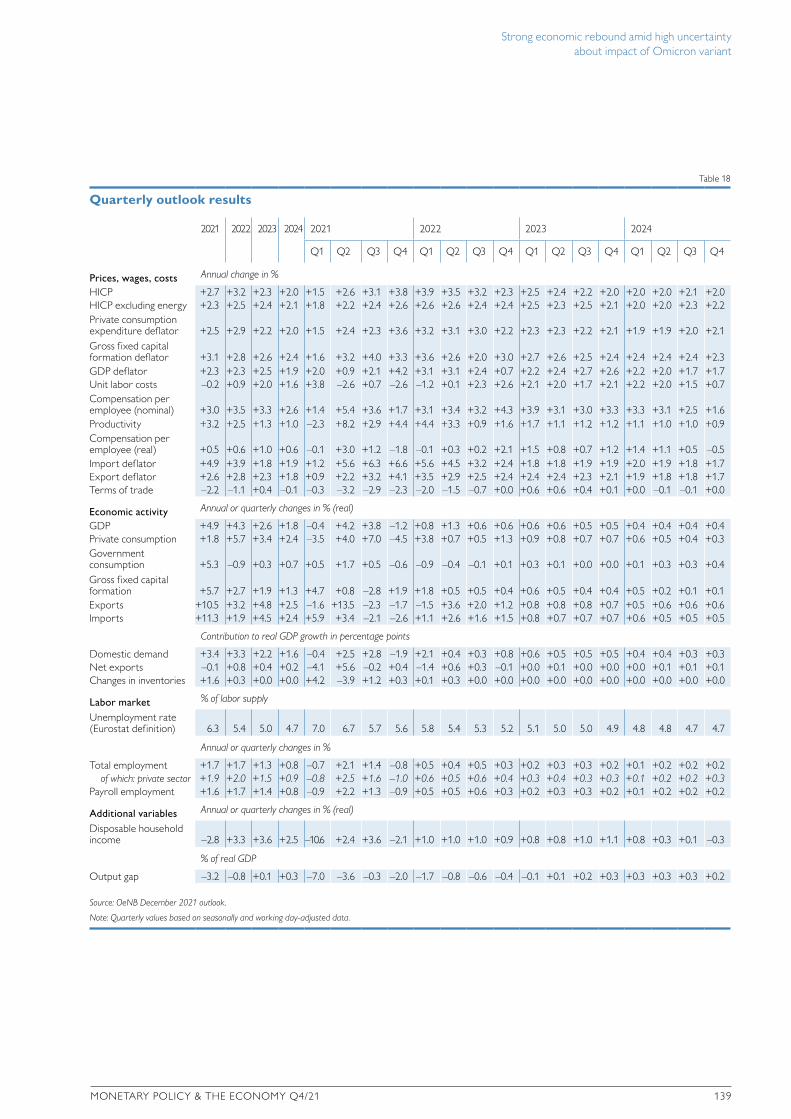
Strong economic rebound amid high uncertainty about impact of Omicron variant
MONETARY POLICY & THE ECONOMY Q4/21 139
Table 17
Current account balance
2020 2021 2022 2023 2024 2020 2021 2022 2023 2024
EUR million % of nominal GDP
Balance of trade 10,899.0 1,361.2 5,241.0 11,221.4 13,839.0 2.9 0.3 1.2 2.5 2.9Balance of goods 3,032.0 –247.2 –1,190.9 454.2 1,994.8 0.8 –0.1 –0.3 0.1 0.4Balance of services 7,867.0 1,608.4 6,431.9 10,767.2 11,844.0 2.1 0.4 1.5 2.4 2.5
Balance of primary income –426.0 –3,480.0 –4,072.0 –3,696.6 –3,718.3 –0.1 –0.9 –0.9 –0.8 –0.8 Balance of secondary income –3,271.0 –3,330.1 –3,340.3 –3,080.8 –3,745.6 –0.9 –0.8 –0.8 –0.7 –0.8 Current account balance 7,202.0 –5,448.9 –2,171.3 4,444.0 6,374.6 1.9 –1.3 –0.5 1.0 1.3
Source: 2020: Statistics Austria; 2021 to 2024: OeNB December 2021 outlook.
Table 18
Quarterly outlook results
2021 2022 2023 2024 2021 2022 2023 2024
Q1 Q2 Q3 Q4 Q1 Q2 Q3 Q4 Q1 Q2 Q3 Q4 Q1 Q2 Q3 Q4
Prices, wages, costs Annual change in %
HICP +2.7 +3.2 +2.3 +2.0 +1.5 +2.6 +3.1 +3.8 +3.9 +3.5 +3.2 +2.3 +2.5 +2.4 +2.2 +2.0 +2.0 +2.0 +2.1 +2.0HICP excluding energy +2.3 +2.5 +2.4 +2.1 +1.8 +2.2 +2.4 +2.6 +2.6 +2.6 +2.4 +2.4 +2.5 +2.3 +2.5 +2.1 +2.0 +2.0 +2.3 +2.2Private consumption expenditure deflator +2.5 +2.9 +2.2 +2.0 +1.5 +2.4 +2.3 +3.6 +3.2 +3.1 +3.0 +2.2 +2.3 +2.3 +2.2 +2.1 +1.9 +1.9 +2.0 +2.1Gross fixed capital formation deflator +3.1 +2.8 +2.6 +2.4 +1.6 +3.2 +4.0 +3.3 +3.6 +2.6 +2.0 +3.0 +2.7 +2.6 +2.5 +2.4 +2.4 +2.4 +2.4 +2.3GDP deflator +2.3 +2.3 +2.5 +1.9 +2.0 +0.9 +2.1 +4.2 +3.1 +3.1 +2.4 +0.7 +2.2 +2.4 +2.7 +2.6 +2.2 +2.0 +1.7 +1.7Unit labor costs –0.2 +0.9 +2.0 +1.6 +3.8 –2.6 +0.7 –2.6 –1.2 +0.1 +2.3 +2.6 +2.1 +2.0 +1.7 +2.1 +2.2 +2.0 +1.5 +0.7Compensation per employee (nominal) +3.0 +3.5 +3.3 +2.6 +1.4 +5.4 +3.6 +1.7 +3.1 +3.4 +3.2 +4.3 +3.9 +3.1 +3.0 +3.3 +3.3 +3.1 +2.5 +1.6Productivity +3.2 +2.5 +1.3 +1.0 –2.3 +8.2 +2.9 +4.4 +4.4 +3.3 +0.9 +1.6 +1.7 +1.1 +1.2 +1.2 +1.1 +1.0 +1.0 +0.9Compensation per employee (real) +0.5 +0.6 +1.0 +0.6 –0.1 +3.0 +1.2 –1.8 –0.1 +0.3 +0.2 +2.1 +1.5 +0.8 +0.7 +1.2 +1.4 +1.1 +0.5 –0.5 Import deflator +4.9 +3.9 +1.8 +1.9 +1.2 +5.6 +6.3 +6.6 +5.6 +4.5 +3.2 +2.4 +1.8 +1.8 +1.9 +1.9 +2.0 +1.9 +1.8 +1.7Export deflator +2.6 +2.8 +2.3 +1.8 +0.9 +2.2 +3.2 +4.1 +3.5 +2.9 +2.5 +2.4 +2.4 +2.4 +2.3 +2.1 +1.9 +1.8 +1.8 +1.7Terms of trade –2.2 –1.1 +0.4 –0.1 –0.3 –3.2 –2.9 –2.3 –2.0 –1.5 –0.7 +0.0 +0.6 +0.6 +0.4 +0.1 +0.0 –0.1 –0.1 +0.0
Economic activity Annual or quarterly changes in % (real)
GDP +4.9 +4.3 +2.6 +1.8 –0.4 +4.2 +3.8 –1.2 +0.8 +1.3 +0.6 +0.6 +0.6 +0.6 +0.5 +0.5 +0.4 +0.4 +0.4 +0.4Private consumption +1.8 +5.7 +3.4 +2.4 –3.5 +4.0 +7.0 –4.5 +3.8 +0.7 +0.5 +1.3 +0.9 +0.8 +0.7 +0.7 +0.6 +0.5 +0.4 +0.3Government consumption +5.3 –0.9 +0.3 +0.7 +0.5 +1.7 +0.5 –0.6 –0.9 –0.4 –0.1 +0.1 +0.3 +0.1 +0.0 +0.0 +0.1 +0.3 +0.3 +0.4Gross fixed capital formation +5.7 +2.7 +1.9 +1.3 +4.7 +0.8 –2.8 +1.9 +1.8 +0.5 +0.5 +0.4 +0.6 +0.5 +0.4 +0.4 +0.5 +0.2 +0.1 +0.1Exports +10.5 +3.2 +4.8 +2.5 –1.6 +13.5 –2.3 –1.7 –1.5 +3.6 +2.0 +1.2 +0.8 +0.8 +0.8 +0.7 +0.5 +0.6 +0.6 +0.6Imports +11.3 +1.9 +4.5 +2.4 +5.9 +3.4 –2.1 –2.6 +1.1 +2.6 +1.6 +1.5 +0.8 +0.7 +0.7 +0.7 +0.6 +0.5 +0.5 +0.5
Contribution to real GDP growth in percentage points
Domestic demand +3.4 +3.3 +2.2 +1.6 –0.4 +2.5 +2.8 –1.9 +2.1 +0.4 +0.3 +0.8 +0.6 +0.5 +0.5 +0.5 +0.4 +0.4 +0.3 +0.3Net exports –0.1 +0.8 +0.4 +0.2 –4.1 +5.6 –0.2 +0.4 –1.4 +0.6 +0.3 –0.1 +0.0 +0.1 +0.0 +0.0 +0.0 +0.1 +0.1 +0.1Changes in inventories +1.6 +0.3 +0.0 +0.0 +4.2 –3.9 +1.2 +0.3 +0.1 +0.3 +0.0 +0.0 +0.0 +0.0 +0.0 +0.0 +0.0 +0.0 +0.0 +0.0
Labor market % of labor supply
Unemployment rate (Eurostat definition) 6.3 5.4 5.0 4.7 7.0 6.7 5.7 5.6 5.8 5.4 5.3 5.2 5.1 5.0 5.0 4.9 4.8 4.8 4.7 4.7
Annual or quarterly changes in %
Total employment +1.7 +1.7 +1.3 +0.8 –0.7 +2.1 +1.4 –0.8 +0.5 +0.4 +0.5 +0.3 +0.2 +0.3 +0.3 +0.2 +0.1 +0.2 +0.2 +0.2of which: private sector +1.9 +2.0 +1.5 +0.9 –0.8 +2.5 +1.6 –1.0 +0.6 +0.5 +0.6 +0.4 +0.3 +0.4 +0.3 +0.3 +0.1 +0.2 +0.2 +0.3
Payroll employment +1.6 +1.7 +1.4 +0.8 –0.9 +2.2 +1.3 –0.9 +0.5 +0.5 +0.6 +0.3 +0.2 +0.3 +0.3 +0.2 +0.1 +0.2 +0.2 +0.2
Additional variables Annual or quarterly changes in % (real)
Disposable household income –2.8 +3.3 +3.6 +2.5 –10.6 +2.4 +3.6 –2.1 +1.0 +1.0 +1.0 +0.9 +0.8 +0.8 +1.0 +1.1 +0.8 +0.3 +0.1 –0.3
% of real GDP
Output gap –3.2 –0.8 +0.1 +0.3 –7.0 –3.6 –0.3 –2.0 –1.7 –0.8 –0.6 –0.4 –0.1 +0.1 +0.2 +0.3 +0.3 +0.3 +0.3 +0.2
Source: OeNB December 2021 outlook.
Note: Quarterly values based on seasonally and working day-adjusted data.

Strong economic rebound amid high uncertainty about impact of Omicron variant
140 OESTERREICHISCHE NATIONALBANK
Table 19
Comparison of current economic forecasts for Austria
OeNB WIFO IHS
December 2021 December 2021 December 2021
2021 2022 2023 2024 2021 2022 2023 2021 2022 2023
Main results Annual change in %
GDP (real) +4.9 +4.3 +2.6 +1.8 +4.1 +5.2 +2.5 +4.3 +4.2 +2.6Private consumption (real) +1.8 +5.7 +3.4 +2.4 +3.4 +6.3 +2.9 +3.2 +5.1 +3.0Government consumption (real) +5.3 –0.9 +0.3 +0.7 +5.3 –2.0 –0.4 +4.0 –0.5 +0.2Gross fixed capital formation (real) +5.7 +2.7 +1.9 +1.3 +5.7 +4.8 +1.8 +6.4 +4.0 +3.0Exports (real) +10.5 +3.2 +4.8 +2.5 +10.2 +8.5 +4.2 +9.2 +7.1 +4.3Imports (real) +11.3 +1.9 +4.5 +2.4 +12.6 +6.1 +3.9 +10.4 +6.7 +4.1Labor productivity1 +3.2 +2.5 +1.3 +1.0 –2.4 +0.7 +0.5 +1.9 +2.2 +1.5
GDP deflator +2.3 +2.3 +2.5 +1.9 +1.6 +2.8 +2.1 +1.5 +2.4 +2.0Consumer price index x x x x +2.8 +3.3 +2.2 +2.8 +2.8 +1.9HICP +2.7 +3.2 +2.3 +2.0 +2.8 +3.4 +2.2 +2.8 +2.8 +1.9Unit labor costs –0.2 +0.9 +2.0 +1.6 +1.1 –0.1 +2.6 +0.2 +1.0 +1.2
Payroll employment2 +1.7 +1.7 +1.3 +0.8 +2.4 +1.9 +1.7 +2.3 +2.0 +1.1
% of labor supply
Unemployment rate3 (Eurostat definition) 6.3 5.4 5.0 4.7 6.4 4.8 4.4 6.4 5.5 5.3
% of nominal GDP
Current account balance –1.3 –0.5 1.0 1.3 –0.8 0.8 0.8 x x x Budget balance (Maastricht definition) –5.9 –2.1 –1.4 –1.1 –6.2 –1.8 –0.6 –5.9 –1.9 –1.3
Technical assumptionsOil price in USD/barrel (Brent) 71.8 77.5 72.3 69.4 71.0 69.0 66.0 71.0 68.0 65.0Short-term interest rate in % –0.5 –0.5 –0.2 0.0 –0.6 –0.4 0.4 –0.5 –0.5 –0.1 USD/EUR exchange rate 1.20 1.10 1.10 1.10 1.18 1.12 1.08 1.18 1.13 1.14
Annual change in %
Euro area GDP (real) +5.1 +4.2 +2.9 +1.6 +5.2 +4.2 +2.4 +5.0 +4.3 +2.2US GDP (real) +5.5 +4.2 +3.0 +2.5 +5.5 +4.4 +2.2 +5.8 +4.0 +2.0World GDP (real) +5.9 +4.4 +3.8 +3.4 x x x +5.6 +4.4 +3.0World trade4 +10.2 +4.5 +4.9 +3.7 x x x +9.5 +3.2 +3.2
Source: OeNB, WIFO, IHS, OECD, IMF, European Commission.
Note: x = no data available.1 OeNB, WIFO: productivity per hour worked; IHS, OECD, European Commission: productivity per employee.2 WIFO, IHS: based on active payroll.3 WIFO: % of persons in payroll employment (national definition).4 IHS: goods according to CPB; European Commission: world imports.
Table 19 continued
Comparison of current economic forecasts for Austria
OECD IMF European Commission
December 2021 October 2021 November 2021
2021 2022 2023 2021 2022 2021 2022 2023
Main results Annual change in %
GDP (real) +4.1 +4.6 +2.5 +3.9 +4.5 +4.4 +4.9 +1.9Private consumption (real) +3.7 +5.8 +2.6 x x +4.2 +6.3 +2.4Government consumption (real) +3.1 +0.2 +0.5 x x +3.4 –0.1 +0.4Gross fixed capital formation (real) +7.9 +4.4 +2.9 x x +8.3 +4.2 +2.3Exports (real) +10.4 +8.1 +5.6 +7.7 +5.3 +8.4 +9.0 +5.4Imports (real) +11.6 +6.9 +5.3 +8.4 +4.6 +9.9 +8.1 +5.7Labor productivity1 x x x x x +2.6 +3.0 +1.2
GDP deflator +1.6 +2.8 +2.1 +2.3 +2.3 +1.8 +2.2 +2.1Consumer price index x x x x x x x x HICP +2.8 +3.0 +2.3 +2.5 +2.4 +2.7 +2.5 +2.0Unit labor costs x x x x x –0.5 –0.7 +1.8
Payroll employment2 x x x +0.6 +1.0 +1.7 +1.9 +0.6
% of labor supply
Unemployment rate3 (Eurostat definition) 5.0 4.7 4.5 6.4 6.0 5.0 4.6 4.5
% of nominal GDP
Current account balance –0.2 0.1 0.3 1.6 2.0 –0.1 –0.2 –0.5 Budget balance (Maastricht definition) –6.3 –2.3 –1.1 –5.8 –2.9 –5.9 –2.3 –1.3
Technical assumptionsOil price in USD/barrel (Brent) 80.0 80.0 80.0 65.7 64.5 71.6 78.9 72.3Short-term interest rate in % x x x –0.5 –0.5 –0.5 –0.5 –0.3 USD/EUR exchange rate 1.20 1.20 1.20 1.20 1.20 1.20 1.20 1.20
Annual change in %
Euro area GDP (real) +5.2 +4.3 +2.5 +5.0 +4.3 +5.0 +4.3 +2.4US GDP (real) +5.6 +3.7 +2.4 +6.0 +5.2 +5.8 +4.5 +2.4World GDP (real) +5.6 +4.5 +3.2 +5.9 +4.9 +5.7 +4.5 +3.5World trade4 +9.3 +4.9 +4.5 +9.7 +6.7 +9.1 +6.4 +4.7
Source: OeNB, WIFO, IHS, OECD, IMF, European Commission.
Note: x = no data available.1 OeNB, WIFO: productivity per hour worked; IHS, OECD, European Commission: productivity per employee.2 WIFO, IHS: based on active payroll.3 WIFO: % of persons in payroll employment (national definition).4 IHS: goods according to CPB; European Commission: world imports.

Strong economic rebound amid high uncertainty about impact of Omicron variant
MONETARY POLICY & THE ECONOMY Q4/21 141
Table 19
Comparison of current economic forecasts for Austria
OeNB WIFO IHS
December 2021 December 2021 December 2021
2021 2022 2023 2024 2021 2022 2023 2021 2022 2023
Main results Annual change in %
GDP (real) +4.9 +4.3 +2.6 +1.8 +4.1 +5.2 +2.5 +4.3 +4.2 +2.6Private consumption (real) +1.8 +5.7 +3.4 +2.4 +3.4 +6.3 +2.9 +3.2 +5.1 +3.0Government consumption (real) +5.3 –0.9 +0.3 +0.7 +5.3 –2.0 –0.4 +4.0 –0.5 +0.2Gross fixed capital formation (real) +5.7 +2.7 +1.9 +1.3 +5.7 +4.8 +1.8 +6.4 +4.0 +3.0Exports (real) +10.5 +3.2 +4.8 +2.5 +10.2 +8.5 +4.2 +9.2 +7.1 +4.3Imports (real) +11.3 +1.9 +4.5 +2.4 +12.6 +6.1 +3.9 +10.4 +6.7 +4.1Labor productivity1 +3.2 +2.5 +1.3 +1.0 –2.4 +0.7 +0.5 +1.9 +2.2 +1.5
GDP deflator +2.3 +2.3 +2.5 +1.9 +1.6 +2.8 +2.1 +1.5 +2.4 +2.0Consumer price index x x x x +2.8 +3.3 +2.2 +2.8 +2.8 +1.9HICP +2.7 +3.2 +2.3 +2.0 +2.8 +3.4 +2.2 +2.8 +2.8 +1.9Unit labor costs –0.2 +0.9 +2.0 +1.6 +1.1 –0.1 +2.6 +0.2 +1.0 +1.2
Payroll employment2 +1.7 +1.7 +1.3 +0.8 +2.4 +1.9 +1.7 +2.3 +2.0 +1.1
% of labor supply
Unemployment rate3 (Eurostat definition) 6.3 5.4 5.0 4.7 6.4 4.8 4.4 6.4 5.5 5.3
% of nominal GDP
Current account balance –1.3 –0.5 1.0 1.3 –0.8 0.8 0.8 x x x Budget balance (Maastricht definition) –5.9 –2.1 –1.4 –1.1 –6.2 –1.8 –0.6 –5.9 –1.9 –1.3
Technical assumptionsOil price in USD/barrel (Brent) 71.8 77.5 72.3 69.4 71.0 69.0 66.0 71.0 68.0 65.0Short-term interest rate in % –0.5 –0.5 –0.2 0.0 –0.6 –0.4 0.4 –0.5 –0.5 –0.1 USD/EUR exchange rate 1.20 1.10 1.10 1.10 1.18 1.12 1.08 1.18 1.13 1.14
Annual change in %
Euro area GDP (real) +5.1 +4.2 +2.9 +1.6 +5.2 +4.2 +2.4 +5.0 +4.3 +2.2US GDP (real) +5.5 +4.2 +3.0 +2.5 +5.5 +4.4 +2.2 +5.8 +4.0 +2.0World GDP (real) +5.9 +4.4 +3.8 +3.4 x x x +5.6 +4.4 +3.0World trade4 +10.2 +4.5 +4.9 +3.7 x x x +9.5 +3.2 +3.2
Source: OeNB, WIFO, IHS, OECD, IMF, European Commission.
Note: x = no data available.1 OeNB, WIFO: productivity per hour worked; IHS, OECD, European Commission: productivity per employee.2 WIFO, IHS: based on active payroll.3 WIFO: % of persons in payroll employment (national definition).4 IHS: goods according to CPB; European Commission: world imports.
Table 19 continued
Comparison of current economic forecasts for Austria
OECD IMF European Commission
December 2021 October 2021 November 2021
2021 2022 2023 2021 2022 2021 2022 2023
Main results Annual change in %
GDP (real) +4.1 +4.6 +2.5 +3.9 +4.5 +4.4 +4.9 +1.9Private consumption (real) +3.7 +5.8 +2.6 x x +4.2 +6.3 +2.4Government consumption (real) +3.1 +0.2 +0.5 x x +3.4 –0.1 +0.4Gross fixed capital formation (real) +7.9 +4.4 +2.9 x x +8.3 +4.2 +2.3Exports (real) +10.4 +8.1 +5.6 +7.7 +5.3 +8.4 +9.0 +5.4Imports (real) +11.6 +6.9 +5.3 +8.4 +4.6 +9.9 +8.1 +5.7Labor productivity1 x x x x x +2.6 +3.0 +1.2
GDP deflator +1.6 +2.8 +2.1 +2.3 +2.3 +1.8 +2.2 +2.1Consumer price index x x x x x x x x HICP +2.8 +3.0 +2.3 +2.5 +2.4 +2.7 +2.5 +2.0Unit labor costs x x x x x –0.5 –0.7 +1.8
Payroll employment2 x x x +0.6 +1.0 +1.7 +1.9 +0.6
% of labor supply
Unemployment rate3 (Eurostat definition) 5.0 4.7 4.5 6.4 6.0 5.0 4.6 4.5
% of nominal GDP
Current account balance –0.2 0.1 0.3 1.6 2.0 –0.1 –0.2 –0.5 Budget balance (Maastricht definition) –6.3 –2.3 –1.1 –5.8 –2.9 –5.9 –2.3 –1.3
Technical assumptionsOil price in USD/barrel (Brent) 80.0 80.0 80.0 65.7 64.5 71.6 78.9 72.3Short-term interest rate in % x x x –0.5 –0.5 –0.5 –0.5 –0.3 USD/EUR exchange rate 1.20 1.20 1.20 1.20 1.20 1.20 1.20 1.20
Annual change in %
Euro area GDP (real) +5.2 +4.3 +2.5 +5.0 +4.3 +5.0 +4.3 +2.4US GDP (real) +5.6 +3.7 +2.4 +6.0 +5.2 +5.8 +4.5 +2.4World GDP (real) +5.6 +4.5 +3.2 +5.9 +4.9 +5.7 +4.5 +3.5World trade4 +9.3 +4.9 +4.5 +9.7 +6.7 +9.1 +6.4 +4.7
Source: OeNB, WIFO, IHS, OECD, IMF, European Commission.
Note: x = no data available.1 OeNB, WIFO: productivity per hour worked; IHS, OECD, European Commission: productivity per employee.2 WIFO, IHS: based on active payroll.3 WIFO: % of persons in payroll employment (national definition).4 IHS: goods according to CPB; European Commission: world imports.


