Embed Size (px)
Citation preview
THÈSE NO 2992 (2004)
ÉCOLE POLYTECHNIQUE FÉDÉRALE DE LAUSANNE
PRÉSENTÉE À LA FACULTÉ INFORMATIQUE ET COMMUNICATIONS
Institut de systèmes de communication
SECTION DES SYSTÈMES DE COMMUNICATION
POUR L'OBTENTION DU GRADE DE DOCTEUR ÈS SCIENCES
PAR
Bachelor of Technology in Electrical Engineering, Indian Institute of Technology, Kanpur, Indeet de nationalité indienne
acceptée sur proposition du jury:
Prof. M. Vetterli, directeur de thèseProf. M. Do, rapporteur
Dr P. Dragotti, rapporteurProf. H. Radha, rapporteurProf. M. Unser, rapporteur
Lausanne, EPFL2004
RATE-DISTORTION OPTIMIZED GEOMETRICALIMAGE PROCESSING
Rahul SHUKLA

Abstract
Since geometrical features, like edges, represent one of the most important per-
ceptual information in an image, efficient exploitation of such geometrical infor-
mation is a key ingredient of many image processing tasks, including compres-
sion, denoising and feature extraction. Therefore, the challenge for the image
processing community is to design efficient geometrical schemes which can cap-
ture the intrinsic geometrical structure of natural images.
This thesis focuses on developing computationally efficient tree based al-
gorithms for attaining the optimal rate-distortion (R-D) behavior for certain
simple classes of geometrical images, such as piecewise polynomial images with
polynomial boundaries. A good approximation of this class allows to develop
good approximation and compression schemes for images with strong geometri-
cal features, and as experimental results show, also for real life images. We first
investigate both the one dimensional (1-D) and two dimensional (2-D) piecewise
polynomials signals. For the 1-D case, our scheme is based on binary tree seg-
mentation of the signal. This scheme approximates the signal segments using
polynomial models and utilizes an R-D optimal bit allocation strategy among
the different signal segments. The scheme further encodes similar neighbors
jointly and is called prune-join algorithm. This allows to achieve the correct ex-
ponentially decaying R-D behavior, D(R) ∼ 2−cR, thus improving over classical
wavelet schemes. We also show that the computational complexity of the scheme
is of O (N log N). We then extend this scheme to the 2-D case using a quadtree,
which also achieves an exponentially decaying R-D behavior, for the piecewise
polynomial image model, with a low computational cost of O (N log N). Again,
the key is an R-D optimized prune and join strategy.
We further analyze the R-D performance of the proposed tree algorithms for
piecewise smooth signals. We show that the proposed algorithms achieve the
oracle like polynomially decaying asymptotic R-D behavior for both the 1-D and
2-D scenarios. Theoretical as well as numerical results show that the proposed
schemes outperform wavelet based coders in the 2-D case.
We then consider two interesting image processing problems, namely de-
noising and stereo image compression, in the framework of the tree structured
segmentation. For the denoising problem, we present a tree based algorithm
which performs denoising by compressing the noisy image and achieves im-
i

ii
proved visual quality by capturing geometrical features, like edges, of images
more precisely compared to wavelet based schemes. We then develop a novel
rate-distortion optimized disparity based coding scheme for stereo images. The
main novelty of the proposed algorithm is that it performs the joint coding of
disparity information and the residual image to achieve better R-D performance
in comparison to standard block based stereo image coder.
Resume
Puisque les elements geometriques, comme les bords, representent des infor-
mation perceptuelles parmi les plus importantes dans une image, l’exploitation
efficace de telles information geometriques dans les images est un ingredient prin-
cipal de nombreuses applications du traitement d’image, y compris la compres-
sion, la reduction du bruit et l’extraction de caracteristiques. Par consequent,
le defi pour la communaute du traitement d’image consiste a concevoir des
methodes geometriques efficaces capables de discerner la structure geometrique
intrinseque des images naturelles.
Cette these se concentre sur le developpement d’algorithmes efficaces bases
sur des arbres pour atteindre le comportement optimal de la fonction rate-
distortion (R-D) pour certaines classes simples d’images geometriques telles
que les images polynomiales par morceaux avec des frontieres polynomiales.
Une bonne approximation de cette classe permet de developper des methodes
d’approximation et de compression efficaces pour des images avec de fortes car-
acteristiques geometriques et egalement, comme les resultats experimentaux
le montrent, pour des images naturelles. Nous etudions d’abord les signaux
polynomiaux par morceaux aussi bien dans une dimension (1-D) que dans deux
dimensions (2-D). Pour le cas 1-D, notre methode est basee sur la segmenta-
tion du signal par arbre binaire. Cette methode fait une approximation des
segments du signal en utilisant des modeles polynomiaux ainsi qu’une strategie
d’attribution des bits aux differents segments du signal qui est optimale au
sens de R-D. En outre, cette methode code des voisins similaires conjointe-
ment et est appelee algorithme tailler-joindre “prune-join”. Ceci nous permet
d’obtenir le comportement de decroissance exponentielle correct au sens de R-
D, D(R) ∼ 2−cR, et de ce fait de surpasser les methodes classiques par on-
delettes. Nous prouvons egalement que la complexite de la methode est de
O (N log N). Nous generalisons ensuite cette methode pour le cas 2-D en util-
isant un ‘quadtree’, ce qui conduit aussi a une decroissance exponentielle de la
fonction R-D pour des images polynomiales par morceaux, avec une complexite
faible de O (N log N). La encore, la solution consiste en une strategie de joindre
et tailler optimisee au sens de R-D.
De plus nous analysons l’efficacite R-D des algorithmes par arbres proposes
pour des signaux regulier par morceaux. Nous montrons que les algorithmes pro-
iii
iv
poses permettent d’obtenir le comportement asymptotique R-D de decroissance
polynomiale, comme celui en presence d’un oracle, aussi bien pour le scenario a
une dimension que pour celui a deux dimensions. Des resultats theoriques ainsi
que numeriques montrent que les methodes proposees surpassent les codeurs par
ondelettes pour le cas 2-D.
Nous considerons ensuite deux problemes interessants de traitement d’image,
a savoir la reduction du bruit et la compression d’images stereo, dans le cadre
de la segmentation par structures d’arbre. Pour le probleme de la reduction du
bruit, nous presentons un algorithme par arbre qui effectue la reduction du bruit
en comprimant l’image bruitee et permet d’obtenir une qualite visuelle amelioree
en discernant des elements geometriques, comme les bords, dans les images avec
plus de precision que les methodes par ondelettes. Nous developpons ensuite
une methode de codage innovatrice basee sur la disparite et optimisee au sens
de R-D. La nouveaute principale de l’algorithme propose consiste dans le fait
qu’il effectue le codage de l’information de disparite et de l’image residuelle
conjointement pour atteindre une efficacite R-D superieure par rapport aux
codeurs classiques d’images stereo par blocs.
Contents
Abstract i
Resume iii
List of Figures viii
List of Tables xii
Acknowledgments xiv
1 Introduction 1
1.1 Motivation . . . . . . . . . . . . . . . . . . . . . . . . . . . . . . . 1
1.2 Related Work . . . . . . . . . . . . . . . . . . . . . . . . . . . . . 3
1.3 Thesis Outline and Contribution . . . . . . . . . . . . . . . . . . . 4
2 Binary Tree Segmentation Algorithms for One Dimensional Piecewise
Polynomial Signals 7
2.1 Motivation . . . . . . . . . . . . . . . . . . . . . . . . . . . . . . . 7
2.2 Binary Tree Algorithms . . . . . . . . . . . . . . . . . . . . . . . . 9
2.3 R-D Analysis of the Oracle Method . . . . . . . . . . . . . . . . . . 13
2.4 R-D Analysis of the Prune Binary Tree Coding Algorithm . . . . . . 13
2.5 R-D Analysis of the Prune-join Binary Tree Algorithm . . . . . . . 17
2.6 Computational Complexity . . . . . . . . . . . . . . . . . . . . . . 19
2.7 Numerical Experiments . . . . . . . . . . . . . . . . . . . . . . . . 21
2.8 Conclusions . . . . . . . . . . . . . . . . . . . . . . . . . . . . . . 22
2.A Proof of Lemma 2.1: Parent Children Pruning . . . . . . . . . . . . 24
2.B Proof of Lemma 2.3: Neighbor Joining . . . . . . . . . . . . . . . 26
2.C R-D Lower-Bound of the Prune Binary Tree Coding Algorithm . . . 27
3 Binary Tree Segmentation Algorithms and 1-D Piecewise Smooth Sig-
nals 31
3.1 Introduction . . . . . . . . . . . . . . . . . . . . . . . . . . . . . . 31
3.2 R-D Analysis for 1-D Smooth Functions . . . . . . . . . . . . . . . 31
3.2.1 R-D Performance of the Oracle Method . . . . . . . . . . . 32
v
vi CONTENTS
3.2.2 R-D Analysis of the Binary Tree Algorithms . . . . . . . . . 32
3.3 R-D Analysis for 1-D Piecewise Smooth Functions . . . . . . . . . . 36
3.3.1 R-D Performance of the Oracle Method . . . . . . . . . . . 36
3.3.2 R-D Analysis of the Binary Tree Algorithms . . . . . . . . . 37
3.4 Simulation Results . . . . . . . . . . . . . . . . . . . . . . . . . . . 39
3.5 Conclusions . . . . . . . . . . . . . . . . . . . . . . . . . . . . . . 40
4 Quadtree Segmentation Algorithms and Piecewise Polynomial Im-
ages 43
4.1 Quadtree Algorithms . . . . . . . . . . . . . . . . . . . . . . . . . 44
4.2 R-D Analysis for the Polygonal Image Model . . . . . . . . . . . . . 46
4.2.1 Image Model and Oracle R-D Performance . . . . . . . . . . 46
4.2.2 R-D Analysis of the Prune Quadtree Algorithm . . . . . . . 47
4.2.3 R-D Analysis of the Prune-join Quadtree Algorithm . . . . . 49
4.3 R-D Analysis for the Piecewise Polynomial Image Model . . . . . . 50
4.3.1 Oracle R-D Performance . . . . . . . . . . . . . . . . . . . 51
4.3.2 R-D Analysis of the Prune Quadtree Algorithm . . . . . . . 56
4.3.3 R-D Analysis of the Prune-join Quadtree Algorithm . . . . . 58
4.4 Computational Complexity . . . . . . . . . . . . . . . . . . . . . . 60
4.5 Simulation Results and Discussion . . . . . . . . . . . . . . . . . . 63
4.6 Conclusions . . . . . . . . . . . . . . . . . . . . . . . . . . . . . . 64
5 Piecewise Smooth Images and Quadtree Segmentation Algorithms 69
5.1 Introduction . . . . . . . . . . . . . . . . . . . . . . . . . . . . . . 69
5.2 R-D Analysis for 2-D Smooth Functions . . . . . . . . . . . . . . . 70
5.3 R-D Analysis for 2-D Piecewise Smooth Functions . . . . . . . . . 74
5.3.1 R-D Analysis for the Horizon Model . . . . . . . . . . . . . 75
5.4 Simulation Results . . . . . . . . . . . . . . . . . . . . . . . . . . . 79
5.5 Conclusions . . . . . . . . . . . . . . . . . . . . . . . . . . . . . . 81
6 New Applications of Tree Algorithms: Denoising and Stereo Image
Coding 83
6.1 Introduction . . . . . . . . . . . . . . . . . . . . . . . . . . . . . . 83
6.2 Denoising Problem . . . . . . . . . . . . . . . . . . . . . . . . . . 84
6.2.1 Simulation Results: Denoising . . . . . . . . . . . . . . . . 86
6.3 Stereo Image Compression . . . . . . . . . . . . . . . . . . . . . . 93
6.3.1 Disparity Dependent Segmentation Based Stereo Image Cod-
ing Algorithm . . . . . . . . . . . . . . . . . . . . . . . . . 94
6.3.2 Simulation Results: Stereo Image Compression . . . . . . . 96
6.4 Discussion . . . . . . . . . . . . . . . . . . . . . . . . . . . . . . . 97
7 Conclusions 101
7.1 Summary . . . . . . . . . . . . . . . . . . . . . . . . . . . . . . . . 101
7.2 Future Research . . . . . . . . . . . . . . . . . . . . . . . . . . . . 102

CONTENTS vii
Bibliography 105
Curriculum Vitae 111

viii CONTENTS
List of Figures
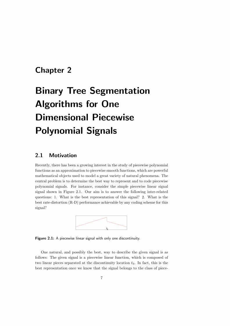
2.1 A piecewise linear signal with only one discontinuity. . . . . . . . 7
2.2 Lagrangian cost based pruning criterion for an operating slope −λ
for each parent node of the tree: Prune the children if (DC1 +
DC2) + λ(RC1 + RC2) ≥ (Dp + λRp). . . . . . . . . . . . . . . . 10
2.3 The prune binary tree segmentation. . . . . . . . . . . . . . . . . 11
2.4 Comparative study of different tree segmentation algorithms. . . 12
2.5 Figure shows the conditions to stop the pruning of a singularity
containing node at the tree level J . That means, J becomes the
tree-depth. . . . . . . . . . . . . . . . . . . . . . . . . . . . . . . 15
2.6 Illustration of the prune-join binary tree joining. . . . . . . . . . 18
2.7 Original and reconstructed piecewise polynomial signals provided
by the prune and prune-join binary tree algorithms. (a) Original
piecewise cubic signal. (b) The prune tree algorithm: MSE=
−35.1 dB, Bit-rate= 0.63 bps. (c) The prune-join tree algorithm:
MSE= −42.20 dB, Bit-rate= 0.59 bps. . . . . . . . . . . . . . . . 22
2.8 Approximations provided by the prune binary tree coding algo-
rithm at different bit-rates. . . . . . . . . . . . . . . . . . . . . . 23
2.9 Approximations provided by the prune-join binary tree coding
algorithm at different bit-rates. . . . . . . . . . . . . . . . . . . . 23
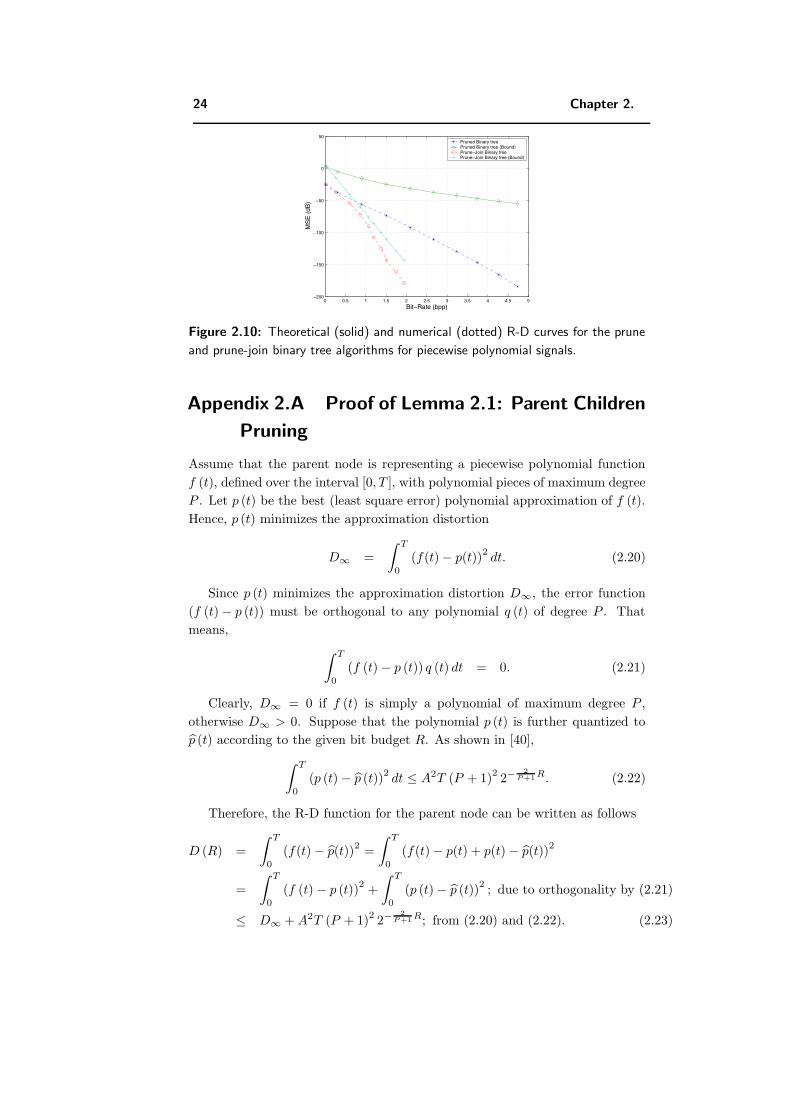
2.10 Theoretical (solid) and numerical (dotted) R-D curves for the
prune and prune-join binary tree algorithms for piecewise poly-
nomial signals. . . . . . . . . . . . . . . . . . . . . . . . . . . . . 24
2.11 The prune binary tree segmentation of a piecewise constant signal
with one singularity. . . . . . . . . . . . . . . . . . . . . . . . . . 27
3.1 Original lena image and its scanned line. . . . . . . . . . . . . . . 36
3.2 Original piecewise smooth signal. . . . . . . . . . . . . . . . . . . 39
3.3 Approximations provided by the prune and prune-join binary tree
coding algorithms. . . . . . . . . . . . . . . . . . . . . . . . . . . 40
3.4 Residual signals provided by the prune and prune-join binary tree
coding algorithms. . . . . . . . . . . . . . . . . . . . . . . . . . . 41
3.5 R-D performance of the prune and prune-join binary tree algo-
rithms for piecewise smooth signals. . . . . . . . . . . . . . . . . 41
ix
x LIST OF FIGURES
3.6 Piecewise polynomial approximations provided by the prune and
prune-join binary tree coding algorithms for a line of the lena
image. . . . . . . . . . . . . . . . . . . . . . . . . . . . . . . . . . 42
4.1 Examples of a black and white (B/W) polygonal image, an edge
tile with a linear boundary, and the quadtree segmentation. . . . 45
4.2 4-connected neighboring nodes. Every neighbor is assigned a two
bit index. . . . . . . . . . . . . . . . . . . . . . . . . . . . . . . . 45
4.3 Examples of the quadtree representation for the polygonal model. 51
4.4 An example of piecewise polynomial image with piecewise poly-
nomial boundaries. Red dots indicate the vertices of piecewise
polynomial singularities. The shown image contains 10 vertices. . 52
4.5 Region of error due to encoding of polynomial boundary with
certain bit rate. . . . . . . . . . . . . . . . . . . . . . . . . . . . 54
4.6 Segmentation performed by the quadtree algorithms for a piece-
wise quadratic image. . . . . . . . . . . . . . . . . . . . . . . . . 61
4.7 Prune-join quadtree tiling for the cameraman image at bi-
trate=0.071 bpp. . . . . . . . . . . . . . . . . . . . . . . . . . . . 65
4.8 Theoretical (solid) and numerical (dotted) R-D curves for the
prune and prune-join quadtree algorithms for the polygonal im-
age class. . . . . . . . . . . . . . . . . . . . . . . . . . . . . . . . 65
4.9 Comparison of the quadtree coder and a wavelet coder
(JPEG2000) for the cameraman image. . . . . . . . . . . . . . . 66
4.10 Residual images of the quadtree coder and JPEG2000 for the
cameraman image at 0.15 bpp. . . . . . . . . . . . . . . . . . . . 66
4.11 R-D performance comparison of the quadtree schemes and
JPEG2000 for the cameraman image. . . . . . . . . . . . . . . . . 67
4.12 Comparison of the quadtree coder and a wavelet coder
(JPEG2000) for the lena image. . . . . . . . . . . . . . . . . . . . 67
4.13 Comparison of artifacts in two regions of the lena image at
0.15 bpp for the prune-join scheme and JPEG2000. . . . . . . . . 68
5.1 Segmentation performed by the quadtree algorithms for a piece-
wise linear image with an elliptical edge. . . . . . . . . . . . . . . 80
5.2 Reconstructed image by JPEG2000 (Rate=.065 bpp, PSNR=
43.81 dB). . . . . . . . . . . . . . . . . . . . . . . . . . . . . . . . 80
5.3 R-D performance comparison of the proposed quadtree algo-
rithms and JPEG2000 for images with smooth elliptical edges. . 81
5.4 Original phantom image along with an encoded image obtained
by JPEG2000. . . . . . . . . . . . . . . . . . . . . . . . . . . . . 82
5.5 Encoded phantom images obtained by the prune and prune-join
quadtree algorithms. . . . . . . . . . . . . . . . . . . . . . . . . . 82
LIST OF FIGURES xi
6.1 R-D curve and its second derivative for a noisy signal. (R0, D0)
represents the knee point of the R-D curve. . . . . . . . . . . . . 85
6.2 Original and noisy piecewise cubic signals. . . . . . . . . . . . . . 86
6.3 Denoising of a noisy piecewise cubic signal using the binary tree
schemes. (a) Original signal. (b) Noisy signal: SNR= 22.44
dB. (c) Prune tree scheme: SNR= 25.62 dB. (d) Prune-join tree
scheme: SNR= 25.57 dB. . . . . . . . . . . . . . . . . . . . . . . 87
6.4 Denoising of a noisy piecewise cubic signal using the wavelet
based schemes. (a) Standard wavelet scheme: SNR= 24.74 dB.
(b) Cycle-spinning based wavelet scheme with hard thresholding:
SNR= 25.53 dB. (c) Cycle-spinning based wavelet scheme with
soft thresholding: SNR= 20.91 dB. . . . . . . . . . . . . . . . . . 88
6.5 SNR performance comparison of the binary tree and wavelet
based schemes for the piecewise cubic signal. . . . . . . . . . . . 88
6.6 Denoising of a noisy signal, constructed from lines of the lena
image, using the binary tree and wavelet based schemes. . . . . . 89
6.7 Original and noisy piecewise quadratic image. For noisy piecewise
quadratic image, SNR= 20.32 dB. . . . . . . . . . . . . . . . . . 90
6.8 Denoised images obtained by the prune and prune-join quadtree
schemes. . . . . . . . . . . . . . . . . . . . . . . . . . . . . . . . . 90
6.9 Denoised images provided by the standard un-decimated wavelet
transform and adaptive directional wavelet transform based
schemes. . . . . . . . . . . . . . . . . . . . . . . . . . . . . . . . . 91
6.10 Original and noisy cameraman image. For noisy cameraman im-
age, SNR= 17.72 dB. . . . . . . . . . . . . . . . . . . . . . . . . 91
6.11 Denoised images obtained by the prune and prune-join quadtree
schemes. . . . . . . . . . . . . . . . . . . . . . . . . . . . . . . . . 92
6.12 Denoised images provided by the standard un-decimated wavelet
transform and adaptive directional wavelet transform based
schemes. . . . . . . . . . . . . . . . . . . . . . . . . . . . . . . . . 92
6.13 The conditional coder/decoder structure proposed by Perkins [38]
for stereo image coding. . . . . . . . . . . . . . . . . . . . . . . . 93
6.14 Original Arch stereo pair. . . . . . . . . . . . . . . . . . . . . . . 97
6.15 Superimposed edge-maps for the Arch stereo pair. . . . . . . . . 97
6.16 Quadtree based disparity map. . . . . . . . . . . . . . . . . . . . 98
6.17 Reconstructed target image along with the segmentation map
obtained by the disparity dependent segmentation based coding
scheme (PSNR=41.4 dB, Bit-rate=0.116 bpp). . . . . . . . . . . 98
6.18 R-D performance comparison of different coding schemes for the
target image of the Arch stereo pair shown in Figure 6.14. . . . . 98

xii LIST OF FIGURES

List of Tables
4.1 Summary of the properties of the different algorithms. . . . . . . 63
4.2 R-D performance comparison of different algorithms for different
images. . . . . . . . . . . . . . . . . . . . . . . . . . . . . . . . . 68
xiii

xiv LIST OF TABLES
Acknowledgements
I would like to sincerely thank my advisor Martin Vetterli for giving me an
opportunity to work on an interesting problem along with the continuous moti-
vation to finish it. I am also greatly indebted to Pier Luigi Dragotti and Minh
Do for their continuous collaboration and guidance, which really help me to
complete this thesis on time. I would also like to thank Hayder Radha for intro-
ducing me to the world of stereo images, which helps me to understand the 3-D
world better. All of them have had a profound impact on my understanding of
how to approach and solve research problems.
I thank all my fellow graduate students and colleagues at EPFL for
their generous help and fruitful discussions, particularly Razvan Cristescu,
Christof Faller, Vladan Velisavljevic, Robert Lee Konsbruck, Patrick Van-
dewalle, Thibaut Ajdler, Williams Devadason, Francoise Behn and Jocelyne
Plantefol. I am also grateful to my Indian friends, Rajesh, Prasenjit, Debjani,
Usha, Anwitaman, Sushil, James and many more, for making my stay at Lau-
sanne comfortable and enjoyable.
Finally, I would like to dedicate this work to my parents, whose constant
support, understanding and encouragement have really brought me here.
xv

Chapter 1
Introduction
1.1 Motivation
From the literature, especially image processing [24], computer vision [2] and
harmonic analysis [5], it is well known that geometrical features, like edges,
represent one of the most important perceptual and objective information in an
image. Thus, the precise modeling of the geometrical information is very crucial
in several image processing applications, like compression, denoising and com-
puter vision. Since edges themselves exhibit a certain degree of smoothness, an
efficient image processing method must be capable of handling the geometrical
regularity of images. Now, the key question of our interest is whether the cur-
rent state of the art wavelet based schemes are able to capture the geometry of
an image efficiently. In the following, we try to understand how well or poorly
wavelet based schemes perform for the compression problem.
In recent years, wavelets have become central to many signal process-
ing applications, in particular approximation and compression. In the latest
wavelet coders and JPEG2000 [61], wavelets are used because of their good
non-linear approximation (NLA) properties for piecewise smooth functions in
one dimension [67]. In 1-D, wavelets derive their good NLA behavior from their
vanishing moment properties [32], and the question now is to see how these prop-
erties carry through in the rate-distortion scenario. Even if good approximation
properties are necessary for good compression, it might not be sufficient. In par-
ticular, in non-linear approximation, the indexing and individual compression
of wavelet coefficients might be inefficient. It is shown for a simpler class of sig-
nals, namely piecewise polynomials, in [9, 40] that the squared error distortion
of wavelet based coders decays as D (R) ∼ d0
√R2−d1
√R. However, since such
a signal can be precisely described by a finite number of parameters, it is not
hard to see that the rate-distortion (R-D) behavior of an oracle based method
1
2 Chapter 1.
decays as1
D(R) ∼ c02−c1R. (1.1)
Thus, even in 1-D, wavelets based schemes perform suboptimally because they
fail to precisely model singularities.
In the 2-D scenario, the situation is much worse. The reason is that wavelets
in 2-D are obtained by a tensor-product of one dimensional wavelets, so they
are adapted only to point singularities and cannot efficiently model the higher
order singularities, like curvilinear singularities, which are abundant in images.
This suggests that wavelets might have some limitation for image processing
applications, especially for compression.
To understand the magnitude of this limitation, consider a simple 2-D func-
tion which is composed of two 2-D polynomials separated by a linear boundary.
Assume that we apply the wavelet transform with enough vanishing moments
on this function. Then, at a level j, the number of significant wavelet coef-
ficients corresponding to 2-D polynomial regions are bounded by a constant
but the number of significant wavelet coefficients representing linear boundary
grows exponentially as 2j. Even if the linear singularity can be represented by
only two parameters, namely slope and intercept, the wavelets based scheme
models it using an exponentially growing number of wavelet coefficients. This
failure to recognize the smoothness of a singularity in 2-D leads to the following
suboptimal R-D behavior [14]
D(R) ∼ log R
R, (1.2)
which is far from the optimal exponentially decaying R-D behavior.2
Since wavelets cannot efficiently model singularities along lines or curves,
wavelet based schemes fail to explore the geometrical structure that is typical
in smooth edges of images. Hence, we need new schemes capable of exploiting
the geometrical information present in images. Therefore, the challenge for
the image coding community is to design efficient geometrical coding schemes.
From an image representation point of view, a number of new schemes have
emerged that attempt to overcome the limitations of wavelets for images with
edge singularities. They include, to name a few, curvelets [5], wedgelets [16],
beamlets [17], contourlets [15], bandelets [37] and edge adaptive geometrical
scheme [10]. Such schemes try to achieve the correct N -term NLA behavior for
certain classes of 2-D functions, which can model images. So far, these schemes
have not led to precise R-D analysis, which is usually more difficult than NLA
analysis.
Moreover, researchers in the wavelet community are also improving wavelet
based schemes. In [47], Romberg et al. presented the wavelet-domain hidden
1In the thesis, we use the term “rate-distortion (R-D)” as a synonym to the term
“distortion-rate (D-R)”.2In Chapter 4, we show that the algorithm proposed in this work achieves an exponentially
decaying R-D behavior for piecewise polynomial images with piecewise polynomial boundaries.
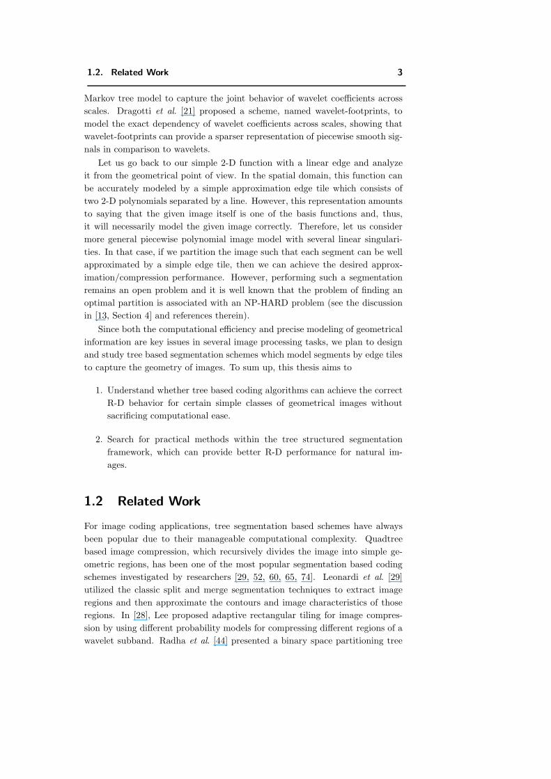
1.2. Related Work 3
Markov tree model to capture the joint behavior of wavelet coefficients across
scales. Dragotti et al. [21] proposed a scheme, named wavelet-footprints, to
model the exact dependency of wavelet coefficients across scales, showing that
wavelet-footprints can provide a sparser representation of piecewise smooth sig-
nals in comparison to wavelets.
Let us go back to our simple 2-D function with a linear edge and analyze
it from the geometrical point of view. In the spatial domain, this function can
be accurately modeled by a simple approximation edge tile which consists of
two 2-D polynomials separated by a line. However, this representation amounts
to saying that the given image itself is one of the basis functions and, thus,
it will necessarily model the given image correctly. Therefore, let us consider
more general piecewise polynomial image model with several linear singulari-
ties. In that case, if we partition the image such that each segment can be well
approximated by a simple edge tile, then we can achieve the desired approx-
imation/compression performance. However, performing such a segmentation
remains an open problem and it is well known that the problem of finding an
optimal partition is associated with an NP-HARD problem (see the discussion
in [13, Section 4] and references therein).
Since both the computational efficiency and precise modeling of geometrical
information are key issues in several image processing tasks, we plan to design
and study tree based segmentation schemes which model segments by edge tiles
to capture the geometry of images. To sum up, this thesis aims to
1. Understand whether tree based coding algorithms can achieve the correct
R-D behavior for certain simple classes of geometrical images without
sacrificing computational ease.
2. Search for practical methods within the tree structured segmentation
framework, which can provide better R-D performance for natural im-
ages.
1.2 Related Work
For image coding applications, tree segmentation based schemes have always
been popular due to their manageable computational complexity. Quadtree
based image compression, which recursively divides the image into simple ge-
ometric regions, has been one of the most popular segmentation based coding
schemes investigated by researchers [29, 52, 60, 65, 74]. Leonardi et al. [29]
utilized the classic split and merge segmentation techniques to extract image
regions and then approximate the contours and image characteristics of those
regions. In [28], Lee proposed adaptive rectangular tiling for image compres-
sion by using different probability models for compressing different regions of a
wavelet subband. Radha et al. [44] presented a binary space partitioning tree
4 Chapter 1.
coding scheme, which employed parent-children pruning for searching the op-
timal tree structure. Recently, Wakin et al. [70] extended the zerotree based
space frequency quantization scheme by adding a wedgelet symbol [16] to its
tree pruning optimization. This enables the scheme to model the joint coherent
behavior of wavelet coefficients near the edges. Another interesting work for
the adaptive edge representations is reported in [66], which employs non-dyadic
rectangular partitioning for the image segmentation.
The tree segmentation based schemes considered in [8, 44, 45, 60, 65, 74]
employ the parent children pruning to obtain the optimal tree structures for the
given bit budget. But they do not attempt to exploit the dependency among
the neighboring nodes with different parents. As we see in the next chapter that
the parent children pruning strategy may not achieve the correct R-D behavior
due to its failure to model the dependency among neighboring nodes.
Recent work closely related to our work is the wedgelets/beamlets based
schemes presented in [16, 17]. These schemes also attempt to capture the geom-
etry of the image by using the linear-edge model explicitly in the approximation
tile. The main focus of these schemes remains the efficient approximation of
edges only without much attention to the efficient coding of smooth surfaces.
However, our work focuses on the efficient representation of both edges and
smooth surfaces to achieve better R-D performance. Another important differ-
ence is that the wedgelets/beamlets based schemes utilize an NLA framework,
whereas we use an R-D framework which is the correct framework for the com-
pression problem.
1.3 Thesis Outline and Contribution
The main goal of this thesis is to design tree structured segmentation based
compression algorithms which can achieve the oracle like R-D performance for
some simple classes of images with computational ease.
The search for an answer to this problem begins in the next chapter which
focuses on 1-D piecewise polynomial signals and presents prune and prune-join
binary tree segmentation based coding algorithms. We analyze the R-D perfor-
mance and computational complexity of these two coding schemes. In particu-
lar, we show that the prune-join tree algorithm, which jointly encodes similar
neighbors, achieves the optimal R-D performance with low computational com-
plexity.
In Chapter 3, we consider more general 1-D piecewise smooth signals and
attempt to understand whether the proposed binary tree segmentation algo-
rithms can accurately model piecewise smooth signals. Our analysis shows that
both the prune and prune-join tree schemes achieve the oracle like polynomially
decaying R-D behavior for piecewise smooth signals.
In Chapter 4, we show the extension of the 1-D scheme to 2-D using a
quadtree based scheme. We consider a piecewise polynomial image model, where
1.3. Thesis Outline and Contribution 5
the edge is also a piecewise polynomial curve. First, we present the oracle R-D
performance which decays exponentially. We then derive the asymptotic R-D
behaviors of the proposed quadtree schemes. Again, we prove that the prune-
join quadtree scheme achieves the oracle like asymptotic R-D performance while
the prune quadtree scheme performs suboptimally. Simulation results show that
the proposed prune-join quadtree coding scheme consistently outperforms state
of the art wavelet based coder (JPEG2000) also in case of compression of real
images like cameraman.
Chapter 5 studies the more complex piecewise smooth images and investi-
gates whether the proposed quadtree based segmentation algorithms can achieve
the correct R-D behavior for these images. Similar to 1-D, the R-D analysis
proves that both the prune and prune-join tree schemes achieve the oracle like
R-D behavior which decays polynomially for piecewise smooth images. Exper-
imental results also confirm the derived R-D behaviors of the quadtree algo-
rithms.
In Chapter 6, we focus on two image processing applications, namely de-
noising and stereo image compression, which require to efficiently exploit the
regularity of both singularities and smooth pieces separated by singularities.
For the denoising problem, we present a solution based on the proposed tree
algorithm and on the key insight that the lossy compression of a noisy signal
can provide the filtered/denoised signal. We then address the problem of stereo
image compression and propose a novel rate-distortion (R-D) optimized dispar-
ity based coding scheme for stereo images. The main novelty of the proposed
scheme is that it performs the joint coding of disparity information and the
residual image to achieve an improved R-D performance.
Finally, we summarize the key results and discuss future research directions
in Chapter 7.

6 Chapter 1.
Chapter 2
Binary Tree Segmentation
Algorithms for One
Dimensional Piecewise
Polynomial Signals
2.1 Motivation
Recently, there has been a growing interest in the study of piecewise polynomial
functions as an approximation to piecewise smooth functions, which are powerful
mathematical objects used to model a great variety of natural phenomena. The
central problem is to determine the best way to represent and to code piecewise
polynomial signals. For instance, consider the simple piecewise linear signal
signal shown in Figure 2.1. Our aim is to answer the following inter-related
questions: 1. What is the best representation of this signal? 2. What is the
best rate-distortion (R-D) performance achievable by any coding scheme for this
signal?
t0
Figure 2.1: A piecewise linear signal with only one discontinuity.
One natural, and possibly the best, way to describe the given signal is as
follows: The given signal is a piecewise linear function, which is composed of
two linear pieces separated at the discontinuity location t0. In fact, this is the
best representation once we know that the signal belongs to the class of piece-
7
8 Chapter 2.
wise polynomials. This signal has a finite number of degrees of freedom, since it
is uniquely determined by the two polynomials and the discontinuity location.
Assume that an oracle provides us the polynomial coefficients and the discon-
tinuity location. Then, a compression algorithm that simply scalar quantizes
these parameters achieves an exponentially decaying R-D behavior (c02−c1R)
at high rates.1 Therefore, the oracle method relies on the correct segmentation
of the signal for achieving the best R-D performance. Thus, the basic ingredi-
ents of the coding scheme are the signal-segmentation and polynomial models
applied to the segments.
But, even for this simple piecewise polynomial signal class, the mean
squared error (MSE) distortion of wavelet based coders decays as D (R) ∼d0
√R2−d1
√R [9, 40]. The reason is that the wavelet based methods perform
independent coding of wavelet coefficients corresponding to a singularity and
so they fail to efficiently model singularities. However, In [40], the oracle like
R-D behavior has been realized with a polynomial computational cost(O(N3
))using dynamic programming (DP). The dynamic segmentation scheme achieves
an exponentially decaying R-D behavior as it performs segmentation accord-
ing to the break points of the signal and codes only the required number of
polynomial pieces. However, due to the exhaustive search for the segmenta-
tion, the dynamic programming algorithm is computationally very expensive.
The above described example, despite its simplicity, reveals the weaknesses of
both wavelet based schemes (suboptimal R-D performance) and dynamic seg-
mentation scheme (high computational cost), and raises the following questions
naturally:
• Can we achieve the oracle like R-D performance with computational ease?
• Can tree segmentation based algorithm mimic the oracle R-D performance
for piecewise polynomial signals?
Therefore, our goal is to design a tree structured compression algorithm based
on the modeling assumption that signals are piecewise smooth functions. In
this case, if we segment the signal into smaller pieces, then each piece can be
well represented by a simpler signal model, which we choose to be a polynomial
function.
This chapter is organized as follows: In the next section, we consider the
pruned binary tree decomposition of the signal, where two children nodes can be
pruned to improve R-D performance. Then, we propose an extension of this al-
gorithm which allows the joint-coding of similar neighboring nodes. To highlight
the intuitions and the main ideas of these algorithms, we present them together
with a toy example (i.e., compression of a piecewise linear signal with one discon-
tinuity). In Sections 2.4 and 2.5, we formally compute the R-D performance of
1In general, for signals with finite number of parameters, an oracle based method will
provide an exponentially decaying R-D behavior at high rates. We will describe the oracle
method in more detail in Section 2.3.
2.2. Binary Tree Algorithms 9
these two coding schemes. Section 2.6 presents their computational complexity.
Most importantly, we show that the prune-join tree algorithm, which jointly
encodes similar neighbors, achieves optimal R-D performance (Theorem 2.2,
Section 2.5) with computational ease ( Section 2.6). In Section 2.7, we present
simulation results which clearly demonstrate that the numerical results follow
the theoretical results proven in the earlier sections. Finally, Section 2.8 offers
concluding remarks.
2.2 Binary Tree Algorithms
In the previous section, we have seen that the wavelet based scheme performs
suboptimally, whereas the dynamic segmentation scheme has high computa-
tional complexity. Thus, both schemes might have some limitations in practice.
That is why, our target is to develop a compression algorithm based on the
binary tree decomposition which achieves the oracle like R-D performance for
piecewise polynomial signals (PPSs) with low computational cost. We first con-
sider the prune binary tree algorithm. This algorithm is similar in spirit to
the algorithm proposed in [45] for searching the best wavelet packet bases. In
our algorithm, each node of the tree is coded independently and, as anticipated
before, each node approximates its signal segment with a polynomial. Finally
the prune tree algorithm utilizes a rate-distortion framework with an MSE dis-
tortion metric. This algorithm can be described as follows:
Algorithm 2.1 The prune binary tree coding algorithm
Step 1: Initialization
1. Segmentation of the input signal using the binary tree decomposition up to
a tree depth J .2
2. Approximation of each node by a polynomial p(t) of degree ≤ P in the least
square error sense.
3. Generation of the R-D curve for each node by approximating the node by
the quantized polynomial p (t), which is obtained by scalar quantizing the poly-
nomial coefficients.3
Step 2: The Lagrangian cost based pruning
4. For the given operating slope −λ, the R-D optimal pruning criterion is as
follows: Prune the children if the sum of the Lagrangian costs of the children
is greater than or equal to the Lagrangian cost of the parent. That means the
children are pruned if (DC1 + DC2) + λ(RC1 + RC2) ≥ (Dp + λRp). This crite-
rion is used recursively to do fast pruning from the full tree depth towards the
root to find the optimal subtree for a given λ [45]. The Lagrangian cost based
2In this work, we use J to indicate the final tree-depth for a given bit-budget, whereas bJindicates the initial chosen depth. Clearly, J ≤ bJ .
3This is best done in an orthogonal basis, that is, the Legendre polynomial basis.
10 Chapter 2.
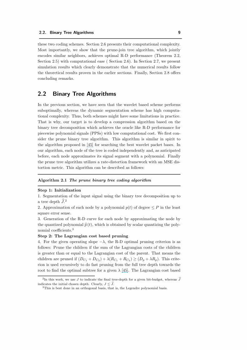
pruning method is illustrated in Figure 2.2.
Left child:
Right child:
Parent Node
R
D
D2
D
R
R
1
1
2
C
C
C
Cp
p
λSlope =−
λSlope =− λSlope =−
Figure 2.2: Lagrangian cost based pruning criterion for an operating slope −λ for
each parent node of the tree: Prune the children if (DC1 +DC2)+λ(RC1 +RC2) ≥(Dp + λRp).
5. Each leaf of the pruned subtree for a given λ has an optimal rate choice
and the corresponding distortion. Summing up the rates of all the tree leaves
along with the tree segmentation cost will provide the overall bit-rate R∗(λ).
Similarly, summing up the associated distortions of all the tree leaves will give
the net distortion D∗(λ).
Step 3: Search for the desired R-D operating slope
The value for λ is determined iteratively until the bit-rate constraint R0 is met
as closely as possible. The search algorithm exploits the convexity of the solution
set and operates as follows [45]:
6. First determine λmin and λmax so that R∗(λmax) ≤ R0 ≤ R∗(λmin).
If the inequality above is an equality for either absolute slope value, then stop.
We have an exact solution, otherwise proceed to the next line.
7. λnew = (D∗(λmin) − D∗(λmax))/(R∗(λmax) − R∗(λmin)).
8. Run the Lagrangian cost based pruning algorithm (Step 2) for λnew.
if (R0 = R∗(λnew)), then the optimum is found. Stop.
elseif (R0 < R∗(λnew)), then λmin = λnew and go to the line 7.
else λmax = λnew and go to the line 7.
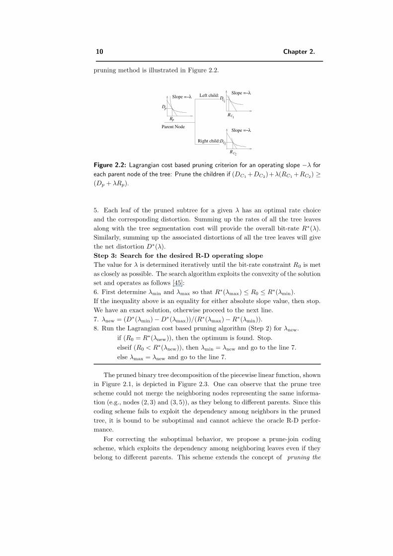
The pruned binary tree decomposition of the piecewise linear function, shown
in Figure 2.1, is depicted in Figure 2.3. One can observe that the prune tree
scheme could not merge the neighboring nodes representing the same informa-
tion (e.g., nodes (2, 3) and (3, 5)), as they belong to different parents. Since this
coding scheme fails to exploit the dependency among neighbors in the pruned
tree, it is bound to be suboptimal and cannot achieve the oracle R-D perfor-
mance.
For correcting the suboptimal behavior, we propose a prune-join coding
scheme, which exploits the dependency among neighboring leaves even if they
belong to different parents. This scheme extends the concept of pruning the
2.2. Binary Tree Algorithms 11
(1,0)
(4,8) (4,9)
(1,1)
(2,3)
(3,5)(3,4)
(2,2)
(0,0)
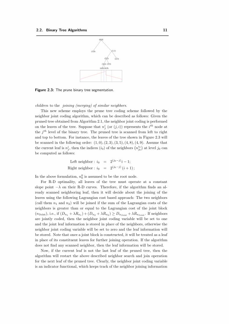
Figure 2.3: The prune binary tree segmentation.
children to the joining (merging) of similar neighbors.
This new scheme employs the prune tree coding scheme followed by the
neighbor joint coding algorithm, which can be described as follows: Given the
pruned tree obtained from Algorithm 2.1, the neighbor joint coding is performed
on the leaves of the tree. Suppose that nij (or (j, i)) represents the ith node at
the jth level of the binary tree. The pruned tree is scanned from left to right
and top to bottom. For instance, the leaves of the tree shown in Figure 2.3 will
be scanned in the following order: (1, 0), (2, 3), (3, 5), (4, 8), (4, 9). Assume that
the current leaf is nij , then the indices (i0) of the neighbors
(ni0
j0
)at level j0 can
be computed as follows:
Left neighbor : i0 = 2(j0−j)i − 1;
Right neighbor : i0 = 2(j0−j) (i + 1) ;
In the above formulation, n00 is assumed to be the root node.
For R-D optimality, all leaves of the tree must operate at a constant
slope point −λ on their R-D curves. Therefore, if the algorithm finds an al-
ready scanned neighboring leaf, then it will decide about the joining of the
leaves using the following Lagrangian cost based approach: The two neighbors
(call them n1 and n2) will be joined if the sum of the Lagrangian costs of the
neighbors is greater than or equal to the Lagrangian cost of the joint block
(nJoint), i.e., if (Dn1 + λRn1) + (Dn2 + λRn2) ≥ DnJoint + λRnJoint . If neighbors
are jointly coded, then the neighbor joint coding variable will be set to one
and the joint leaf information is stored in place of the neighbors, otherwise the
neighbor joint coding variable will be set to zero and the leaf information will
be stored. Note that once a joint block is constructed, it will be treated as a leaf
in place of its constituent leaves for further joining operation. If the algorithm
does not find any scanned neighbor, then the leaf information will be stored.
Now, if the current leaf is not the last leaf of the pruned tree, then the
algorithm will restart the above described neighbor search and join operation
for the next leaf of the pruned tree. Clearly, the neighbor joint coding variable
is an indicator functional, which keeps track of the neighbor joining information
12 Chapter 2.
of the pruned tree leaves. Thus, each leaf has a binary neighbor joint coding
variable, which indicates whether it is jointly coded or not. The prune-join
coding scheme can be summarized as follows:
Algorithm 2.2 The prune-join binary tree coding algorithm
Step 1: Initialization
Following Steps 1 and 2 of Algorithm 2.1, find the best pruned tree for a given
λ.
Step 2: The neighbor joint coding algorithm
Given the pruned tree, perform the joint coding of similar neighboring leaves
as explained above. That means, the two neighbors will be joined if the sum of
the Lagrangian costs of the neighbors is greater than or equal to the Lagrangian
cost of the joint block, i.e., if (Dn1 + λRn1)+(Dn2 + λRn2) ≥ DnJoint +λRnJoint .
Step 3: Search for the desired R-D operating slope
Similar to Algorithm 2.1, iterate the process over λ until the bit budget con-
straint is met.
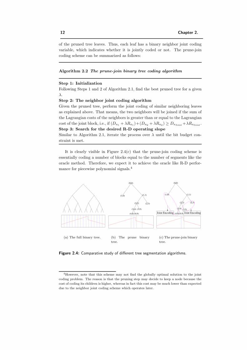
It is clearly visible in Figure 2.4(c) that the prune-join coding scheme is
essentially coding a number of blocks equal to the number of segments like the
oracle method. Therefore, we expect it to achieve the oracle like R-D perfor-
mance for piecewise polynomial signals.4
(a) The full binary tree.
(1,0)
(4,8) (4,9)
(1,1)
(2,3)
(3,5)(3,4)
(2,2)
(0,0)
(b) The prune binary
tree.
(2,3)
(4,8)(4,9)
(3,4) (3,5)
(0,0)
(2,2)
(1,0) (1,1)
Joint Encoding Joint Encoding
(c) The prune-join binary
tree.
Figure 2.4: Comparative study of different tree segmentation algorithms.
4However, note that this scheme may not find the globally optimal solution to the joint
coding problem. The reason is that the pruning step may decide to keep a node because the
cost of coding its children is higher, whereas in fact this cost may be much lower than expected
due to the neighbor joint coding scheme which operates later.
2.3. R-D Analysis of the Oracle Method 13
2.3 R-D Analysis of the Oracle Method
Consider a continuous-time piecewise polynomial signal f(t), defined over the
interval [0, T ], which contains S internal singularities. Assume that the function
f(t) is bounded in magnitude by some constant A and the maximum degree of
a polynomial piece is P . The signal is uniquely determined by (S + 1) polyno-
mials and by S internal singularities. That means such a signal can be precisely
described by a finite number of parameters. Suppose that the values for the
parameters of the polynomial pieces, and the locations of the internal singulari-
ties are provided with arbitrary accuracy by an oracle. In that case, it has been
shown in [40] that the R-D behavior of the oracle based method decays as
D(R) ≤ c02−c1R, (2.1)
where c0 = 2A2T (S + 1)(P + 1)2 and c1 = 2(P+3)(S+1) .
2.4 R-D Analysis of the Prune Binary Tree Coding
Algorithm
This section presents the asymptotic R-D behavior of the prune tree coding
algorithm for piecewise polynomial signals. We compute the worst case R-D
upper-bound in the operational (algorithmic) sense.5 This is to gain insight into
the algorithm’s performance at high rates and because it is difficult to compute
the exact R-D function in a general setting such as ours.6 First, we state a simple
result in the form of Lemma 2.1 that the Lagrangian cost based pruning will
prune the children nodes if the parent node has no singularity. Then we show
that the prune tree algorithm encodes a number of leaves which grows linearly
with respect to the decomposition depth J . This implies that several nodes
with same parameters are coded separately (e.g., see Figure 2.4(b)). Finally,
we prove that this independent coding of similar leaves results in a suboptimal
R-D behavior given by Theorem 2.1.
Lemma 2.1 At high bit rates, the Lagrangian cost (L = D (R) + λR) based tree
pruning method prunes the children nodes if and only if the parent node does
not contain a singularity.
Proof: see Appendix 2.A.
An intuitive explanation of the above result is as follows: If the parent node
does not have a singularity, then its decomposition leads to the repetitive coding
of the same polynomial, which is clearly suboptimal. And if the parent node
5Note that this differs from classic R-D theory, where exact (or tight upper/lower bounds)
R-D behavior is computed for some exemplary processes.6However, we also present the expected R-D lower-bound of the prune tree algorithm for
piecewise constant signals with only one discontinuity in Appendix 2.C.
14 Chapter 2.
contains a singularity, then its decomposition provides better approximation,
which will clearly improve the R-D performance at high rates.
Lemma 2.2 The bottom-up R-D optimal pruning method results in a binary
tree with the number of leaves upper-bounded by (J + 1)S, where J and S repre-
sent the final tree-depth and the number of internal singularities in the piecewise
polynomial signal, respectively.
Proof: Since we are interested in the asymptotic R-D behavior, we will consider
the worst case scenario. As the signal has only S transition points, at most S
tree nodes at a tree level will have a transition point and the remaining nodes will
be simply represented by a polynomial piece without any discontinuity. Clearly,
at high rates, for achieving better R-D performance the tree pruning scheme
will only split nodes with singular points, as they cannot be well approximated
by a polynomial (Lemma 2.1). This means that every level, except the levels
j = 0 and J , will generate at most S leaves. The level J will have 2S leaves,
while the level 0 cannot have any leaf at high rates for S > 0. Hence, the total
number N0 of leaves in the pruned binary tree is
N0 ≤ 2S + (J − 1)S = (J + 1)S. (2.2)
Therefore, the number of leaves to be coded grows linearly with respect to
the depth J .
Moreover, it can also be noted that in the pruned tree, every tree level can
have at most 2S nodes. Hence, the total number M0 of nodes in the pruned
tree can be given as follows
M0 ≤ 2JS + 1. (2.3)
Theorem 2.1 The prune binary tree coding algorithm, which employs the
bottom-up R-D optimization using parent-children pruning, achieves the follow-
ing asymptotic R-D behavior
DP (R) ≤ c2
√R2−c3
√R, (2.4)
where c2 = 16A2TS (P + 1)2√
4(P+1)S and c3 =
√4
(P+1)S , for piecewise poly-
nomials signals.
Proof: Since the piecewise polynomial function f (t) has only S transition
points, at most S leaves will have a transition point and the remaining JS
leaves (Lemma 2.2) can be simply represented by a polynomial piece without
any discontinuity. At high rates, leaves with singular points will be at the tree
depth J , so the size of each of them will be T 2−J . The distortion of each of
these leaves can be bounded by A2T 2−J ≤ A2T (P + 1)22−J and it will not
decrease with the rate. This is because simple polynomials cannot represent
piecewise polynomial functions, so we approximate leaves with singularities by
2.4. R-D Analysis of the Prune Binary Tree Coding Algorithm 15
the zero polynomial. Leaves without singularities can be well approximated by
a polynomial. In particular, a leaf l at tree level j is of size Tl = T 2−j and
its R-D function can be bounded by Dl = A2 (P + 1)2Tl2
− 2P+1 Rl [40]. Since
R-D optimal solution of exponentially decaying R-D functions results in equal
distortion for each leaf [12], the coding algorithm will allocate the same rate Rj
to all the leaves without singularities at the same tree level j. As R-D optimality
requires that leaves without singularities operate at a constant slope −λ on their
R-D curves, we have
∂Dj
∂Rj= −λ, ∀j ≥ 0
⇒ A2 (P + 1)2 T 2−j2−2
P+1 Rj =(P + 1)λ
2 ln 2. (2.5)
Equation (2.5) is essentially the equal distortion constraint. Let Rj and Rk
be the rates allocated to the leaves without singularities at levels j and k,
respectively. The equal distortion constraint for the leaves without singularities
at tree levels j and k means that
A2 (P + 1)2T 2−j2−
2P+1 Rj = A2 (P + 1)
2T 2−k2−
2P+1 Rk
⇒ Rj = Rk +P + 1
2(k − j). (2.6)
⇒ RJ+1 = RJ − P + 1
2≤ RJ , (2.7)
where RJ and RJ+1 represent the rates allocated to leaves without singularities
at levels J and J + 1, respectively. Note that the nodes with singularities will
be allocated zero rate.7
: Node with a singularity
: Node without singularity
Tree Level
J+1
J
J−1
Do not prune.
Prune.
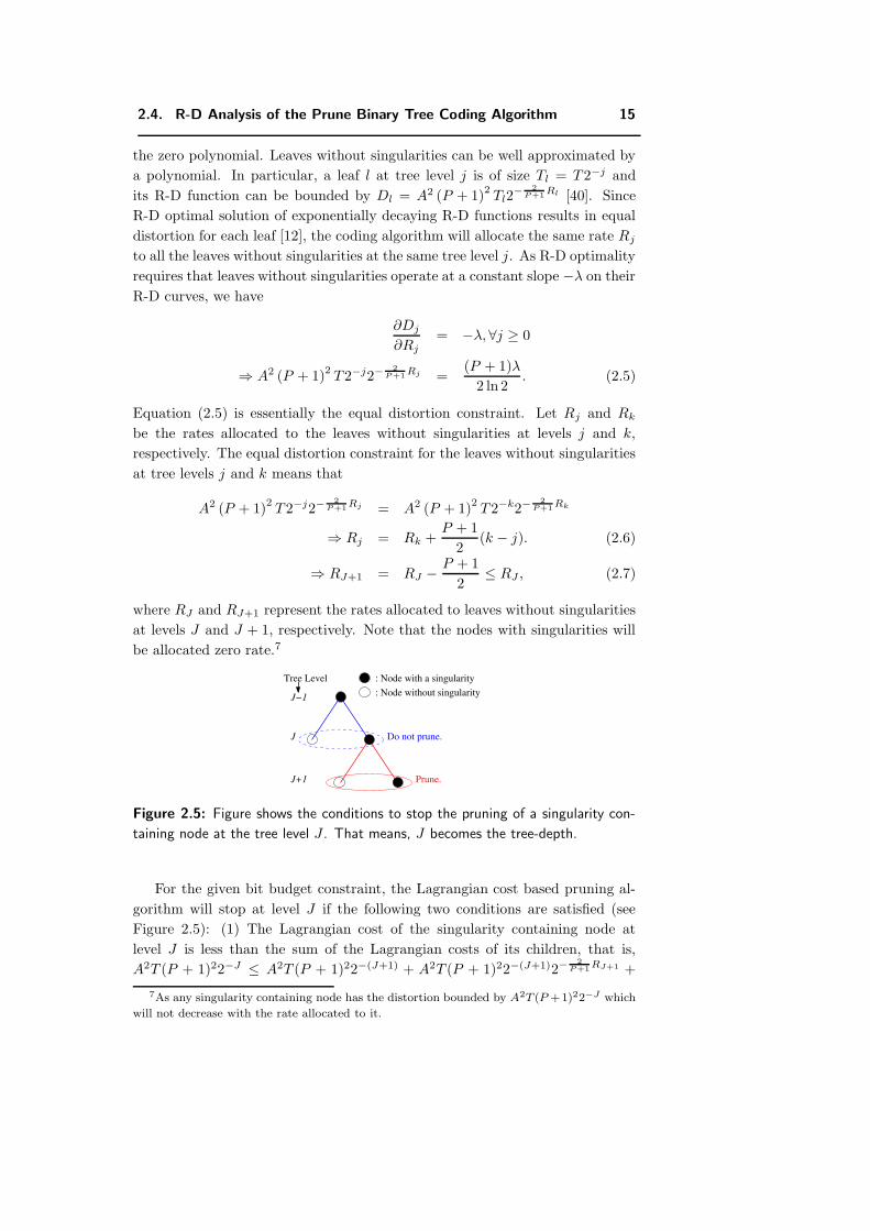
Figure 2.5: Figure shows the conditions to stop the pruning of a singularity con-
taining node at the tree level J . That means, J becomes the tree-depth.
For the given bit budget constraint, the Lagrangian cost based pruning al-
gorithm will stop at level J if the following two conditions are satisfied (see
Figure 2.5): (1) The Lagrangian cost of the singularity containing node at
level J is less than the sum of the Lagrangian costs of its children, that is,
A2T (P + 1)22−J ≤ A2T (P + 1)22−(J+1) + A2T (P + 1)22−(J+1)2−2
P+1 RJ+1 +
7As any singularity containing node has the distortion bounded by A2T (P +1)22−J which
will not decrease with the rate allocated to it.
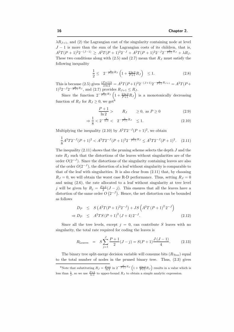
16 Chapter 2.
λRJ+1, and (2) the Lagrangian cost of the singularity containing node at level
J − 1 is more than the sum of the Lagrangian costs of its children, that is,
A2T (P + 1)22−(J−1) ≥ A2T (P + 1)22−J + A2T (P + 1)22−J2−2
P+1 RJ + λRJ .
These two conditions along with (2.5) and (2.7) mean that RJ must satisfy the
following inequality
1
2≤ 2−
2P+1 RJ
(1 + 2 ln 2
P+1 RJ
)≤ 1. (2.8)
This is because (2.5) gives (P+1)λ2 ln 2 = A2T (P +1)22−(J+1)2−
2P+1 RJ+1 = A2T (P +
1)22−J2−2
P+1RJ , and (2.7) provides RJ+1 ≤ RJ .
Since the function 2−2
P+1 RJ
(1 + 2 ln 2
P+1 RJ
)is a monotonically decreasing
function of RJ for RJ ≥ 0, we get8
P + 1
ln 2> RJ ≥ 0, as P ≥ 0 (2.9)
⇒ 1
8< 2−
2ln 2 < 2−
2P+1 RJ ≤ 1. (2.10)
Multiplying the inequality (2.10) by A2T 2−J(P + 1)2, we obtain
1
8A2T 2−J(P + 1)2 < A2T 2−J(P + 1)22−
2P+1 RJ ≤ A2T 2−J(P + 1)2. (2.11)
The inequality (2.11) shows that the pruning scheme selects the depth J and the
rate RJ such that the distortions of the leaves without singularities are of the
order O(2−J ). Since the distortions of the singularity containing leaves are also
of the order O(2−J), the distortion of a leaf without singularity is comparable to
that of the leaf with singularities. It is also clear from (2.11) that, by choosing
RJ = 0, we will obtain the worst case R-D performance. Thus, setting RJ = 0
and using (2.6), the rate allocated to a leaf without singularity at tree level
j will be given by Rj = P+12 (J − j). This ensures that all the leaves have a
distortion of the same order O(2−J
). Hence, the net distortion can be bounded
as follows
DP ≤ S(A2T (P + 1)22−J
)+ JS
(A2T (P + 1)
22−J
)⇒ DP ≤ A2TS (P + 1)
2(J + 4) 2−J . (2.12)
Since all the tree levels, except j = 0, can contribute S leaves with no
singularity, the total rate required for coding the leaves is
RLeaves = S
J∑j=1
P + 1
2(J − j) = S(P + 1)
J (J − 1)
4. (2.13)
The binary tree split-merge decision variable will consume bits (RTree) equal
to the total number of nodes in the pruned binary tree. Thus, (2.3) gives
8Note that substituting RJ = P+1ln 2
in 2− 2
P+1RJ
“1 + 2 ln 2
P+1RJ
”results in a value which is
less than 12, so we use P+1
ln 2to upper-bound RJ to obtain a simple analytic expression.
2.5. R-D Analysis of the Prune-join Binary Tree Algorithm 17
RTree ≤ 2JS + 1. The total bit rate can be seen as the sum of the costs of
coding the binary tree itself and the quantized model parameters of the leaves.
Hence, the total bit rate can be written as follows
R = RTree + RLeaves ≤ 2JS + 1 +(P + 1)S
4J (J − 1)
⇒ R ≤ (P + 1)S
4(J + 4)
2; as S > 0 and J is large. (2.14)
Combining (2.12) and (2.14) by eliminating J and noting that the right hand
side of (2.12) is a decreasing function of J , whereas the right hand side of (2.14)
is an increasing function of J , we obtain the following R-D bound
DP ≤ 16A2TS (P + 1)2
√4
(P + 1)SR2
−q
4(P+1)S
R.
Therefore, the prune binary tree algorithm exhibits the announced decay.
2.5 R-D Analysis of the Prune-join Binary Tree Al-
gorithm
Before proving that the prune-join coding scheme achieves the oracle like asymp-
totic R-D behavior in the operational sense, we show that this coding scheme
encodes a number of leaves which remains fixed with respect to the tree depth J .
Lemma 2.3 At high bit rates, the Lagrangian cost based joining method jointly
codes two neighboring nodes of the binary tree, if and only if the joint node has
no singularity.
Proof: see Appendix 2.B.
An intuitive explanation is as follows: If the joint node has no singularity,
then neighboring nodes are essentially characterized by the same polynomial.
Thus, joining of these nodes will improve the R-D performance by avoiding
the repetitive coding of same information. On the other hand, if the joint node
contains singularities, then separate coding of neighboring nodes provides better
approximation and, thus, improves the R-D performance at high rates.
Lemma 2.4 The prune-join binary tree algorithm, which jointly encodes sim-
ilar neighbors, reduces the effective number of leaves to be encoded to S + 1,
where S is the number of the internal singular points in the piecewise polyno-
mial signal.
Proof: Lemma 2.3 guarantees that the neighboring leaves will be joined to
improve the R-D performance if the joint block does not have a singularity. In
particular, if J is large enough, each singularity will lie on a different dyadic
leaf. Therefore, as a consequence of neighbor joining, all the leaves between
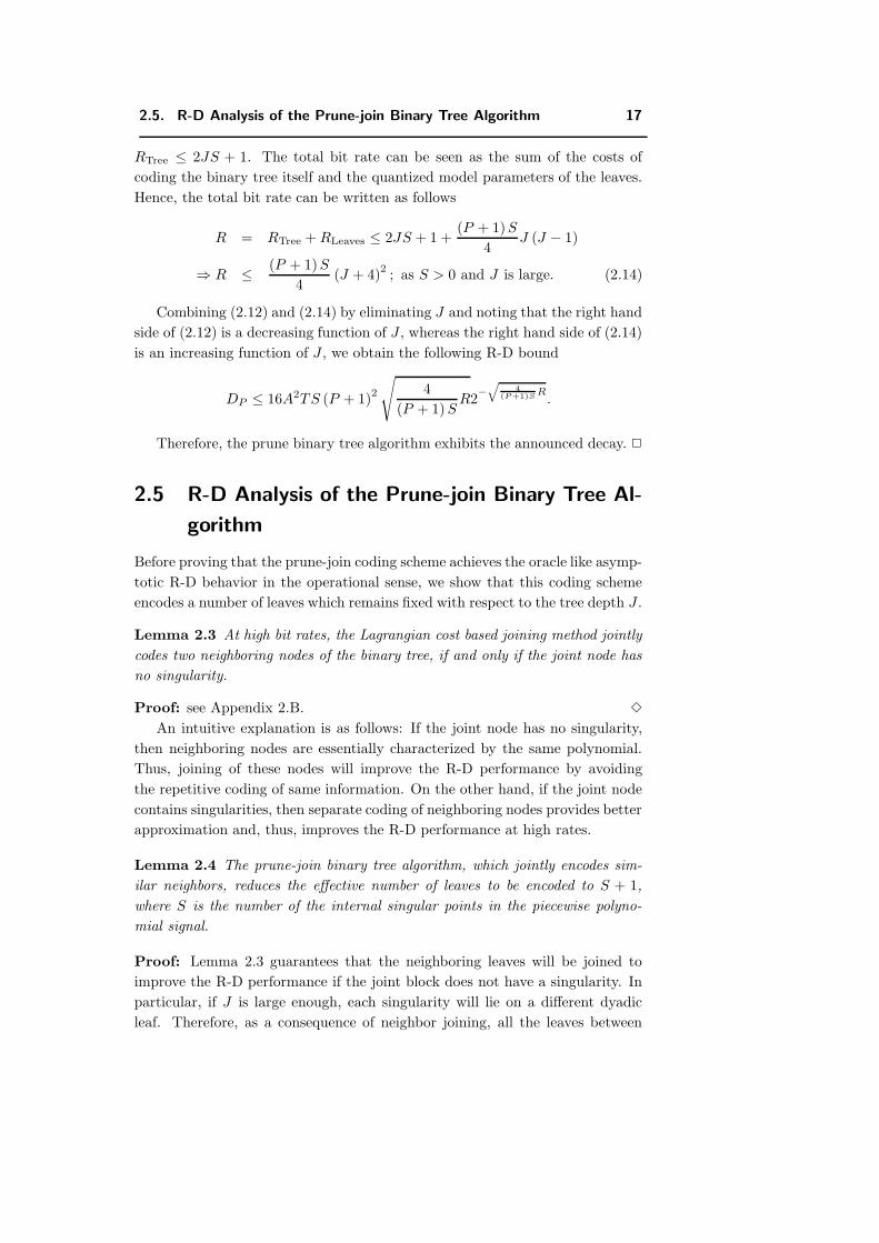
18 Chapter 2.
any two consecutive singularity containing leaves will be joined to form a single
joint block (see the example in Figure 2.6). Thus, the prune-join tree algorithm
results in S + 1 joint leaves and S leaves with a singularity. Since the leaves
containing a singularity will not be encoded, the number of encoded leaves
becomes S + 1. This means that the number of leaves to be coded remains
constant with respect to the tree depth J .
(4,9)(4,8)
(2,2)
(1,0) (1,1)
(3,5)(3,4)
(2,3)
(0,0)
Joint Encoding
(a) Joining of left leaves.
(0,0)
(2,3)
(4,8)(4,9)
(3,4)
(2,2)
(3,5)
(1,0) (1,1)
Joint Encoding
(b) Joining of right
leaves.
(4,8)(4,9)
(3,4) (3,5)
(2,2)
(1,0) (1,1)
(2,3)
(0,0)
Joint Encoding Joint Encoding
(c) Complete joining.
Figure 2.6: Illustration of the prune-join binary tree joining.
Theorem 2.2 The prune-join binary tree algorithm, which jointly encodes sim-
ilar neighbors, achieves the oracle like exponentially decaying asymptotic R-D
behavior
DPJ (R) ≤ c42−c5R, (2.15)
where c4 = 2A2T (2S + 1) (P + 1)2
and c5 = 2(S(P+7)+(P+1)) , for piecewise poly-
nomial signals.
Proof: The prune-join binary tree algorithm provides (S + 1) joint blocks and
at most S leaves with a singularity. The distortion of the leaves with singularities
is bounded by A2T 2−J ≤ A2T (P + 1)22−J and it does not decrease with the
rate (recall that the algorithm approximates singularity containing blocks with
the zero polynomial). The size of each joint block can be bounded by T . Thus,
the distortion of each joint block is bounded by A2 (P + 1)2 T 2−2
P+1 Rl , where Rl
is the rate allocated to that block. Again, R-D optimization forces all the joint
blocks to have the same distortion. As for the prune tree algorithm, one can show
that R-D optimization results in a tree-depth J and a bit allocation strategy
such that the joint blocks and the singularity containing leaves have a distortion
of the same order O(2−J
). This means that the algorithm allocates (P+1)
2 J bits
to each joint block and no bits to the leaves with singularities. Thus, the total
rate required for coding the joint leaves is given by RLeaves = (S + 1) (P+1)2 J .
2.6. Computational Complexity 19
In the prune-join coding scheme, the side information consists of two parts:
1. Bits required to code the pruned tree (RTree). 2. Bits required to code the
leaf joint coding tree (RLeafJointCoding). The tree split-merge variable needs bits
equal to the total number of nodes in the pruned tree, whereas the joint coding
decision variable requires bits equal to the total number of leaves in the pruned
tree. Hence, RTree ≤ 2JS + 1 (from (2.3)), and RLeafJointCoding ≤ (J + 1)S
(from (2.2)). The total bit rate is the sum of the costs of coding the binary tree
itself, the leaves joint coding information and the quantized model parameters
of the leaves. Thus, the total bit rate can be written as follows
R = RTree + RLeafJointCoding + RLeaves
R ≤ 2JS + 1 + (J + 1)S + (S + 1)(P + 1)
2J (2.16)
⇒ R ≤ (S (P + 7) + (P + 1))
2(J + 1). (2.17)
The net distortion bound is as follows
DPJ ≤ SA2T (P + 1)22−J + (S + 1)A2T (P + 1)22−J
= (2S + 1) (P + 1)2A2T 2−J = c42
−(J+1)
⇒ DPJ ≤ c42− 2
(S(P+7)+(P+1)) R; from (2.17).
Therefore, the prune-join tree algorithm achieves an exponentially decaying R-D
behavior.
Note that the R-D behavior of the prune-join tree scheme is worse than that
of the oracle method given by (2.1). One can notice in (2.16) that the prune-join
tree scheme needs RTree = (2JS + 1) bits to code the tree-segmentation infor-
mation, which causes the divergence in the R-D performance of the proposed
tree scheme and that of the oracle method.
Remark: Note that the prune tree scheme is the best in the operational
R-D sense, due to the Lagrangian pruning, among all algorithms that code the
dyadic segments independently. But this scheme fails to achieve the correct
R-D behavior, as it cannot join the similar neighbors with different parents. On
the other hand, although we cannot claim that the prune-join scheme is the
best among all joint coding schemes, it achieves an exponentially decaying R-D
behavior for piecewise polynomial signals as the prune-join scheme is capable of
joining the similar neighbors.
2.6 Computational Complexity
For the complexity analysis, we consider a discrete-time signal of size N . The
complete prune tree algorithm essentially performs three operations:
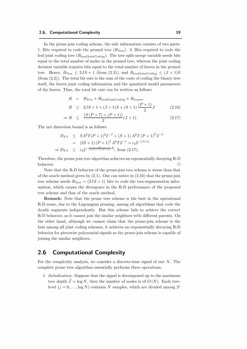
1. Initialization: Suppose that the signal is decomposed up to the maximum
tree depth J = log N , then the number of nodes is of O (N). Each tree-
level (j = 0, . . . , log N) contains N samples, which are divided among 2j
20 Chapter 2.
nodes. Hence, the average size of nodes is of O (log N). Initialization
basically consists of the following operations:
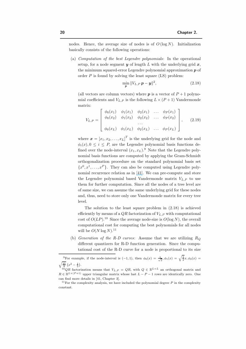
(a) Computation of the best Legendre polynomials: In the operational
setup, for a node segment y of length L with the underlying grid x,
the minimum squared-error Legendre polynomial approximation p of
order P is found by solving the least square (LS) problem:
minp
‖VL,P p − y‖2, (2.18)
(all vectors are column vectors) where p is a vector of P + 1 polyno-
mial coefficients and VL,P is the following L× (P + 1) Vandermonde
matrix:
VL,P =
φ0(x1) φ1(x1) φ2(x1) . . . φP (x1)
φ0(x2) φ1(x2) φ2(x2) . . . φP (x2)
. . .
φ0(xL) φ1(xL) φ2(xL) . . . φP (xL)
, (2.19)
where x = [x1, x2, . . . , xL]T
is the underlying grid for the node and
φi(x), 0 ≤ i ≤ P, are the Legendre polynomial basis functions de-
fined over the node-interval (x1, xL).9 Note that the Legendre poly-
nomial basis functions are computed by applying the Gram-Schmidt
orthogonalization procedure on the standard polynomial basis set
x0, x1, . . . , xP . They can also be computed using Legendre poly-
nomial recurrence relation as in [41]. We can pre-compute and store
the Legendre polynomial based Vandermonde matrix VL,P to use
them for further computation. Since all the nodes of a tree level are
of same size, we can assume the same underlying grid for these nodes
and, thus, need to store only one Vandermonde matrix for every tree
level.
The solution to the least square problem in (2.18) is achieved
efficiently by means of a QR factorization of VL,P with computational
cost of O(LP ).10 Since the average node-size is O(log N), the overall
computational cost for computing the best polynomials for all nodes
will be O(N log N).11
(b) Generation of the R-D curves : Assume that we are utilizing RQ
different quantizers for R-D function generation. Since the compu-
tational cost of the R-D curve for a node is proportional to its size
9For example, if the node-interval is (−1, 1), then φ0(x) = 1√2, φ1(x) =
q32x, φ2(x) =q
458
`x2 − 1
3
´.
10QR factorization means that VL,P = QR, with Q ∈ RL×L an orthogonal matrix and
R ∈ RL×(P+1) upper triangular matrix whose last L − P − 1 rows are identically zero. One
can find more details in [41, Chapter 3].11For the complexity analysis, we have included the polynomial degree P in the complexity
constant.
2.7. Numerical Experiments 21
and the number of quantizers used, the overall cost of computing the
R-D curves for all the tree nodes is O (NRQ log N).
Therefore, the overall cost of computing the best polynomials and R-D
curves for all the tree nodes is O (NRQ log N).
2. Pruning algorithm requires to compute the minimum Lagrangian cost at
each node for the chosen operating slope −λ. This results in a computa-
tional cost of O (N log RQ) due to the binary search through the convex
R-D curve of each node. The algorithm also performs split-merge decision
at the nodes, which requires a computational cost of O (N). Hence, the
pruning algorithm has the computational cost of O (N log RQ).
3. Iterative search algorithm for an optimal operating slope calls the pruning
algorithm for the chosen operating slope −λ. Our bisection search scheme
obtains the optimal operating slope in O (log N) iterations [45]. Thus, the
computational cost of this scheme is O (N log RQ log N).
Hence, the complete computational complexity CPrune of the prune tree algo-
rithm is
CPrune = O (NRQ log N) + O (N log RQ log N) O (NRQ log N) .
Since a pruned binary tree has a number of leaves of O(log N) (J ≤ log N and
eq. (2.2)) and the size of any leaf is bounded by O(N), the computational cost
of the neighbor joint coding algorithm will be O (NRQ log N). The prune-join
coding scheme employs the prune tree algorithm followed by the neighbor joint
coding algorithm. Hence, the overall computational complexity of the prune-join
coding scheme is the sum of the computational costs of the prune tree scheme
and the neighbor joint coding scheme. Therefore, the overall computational
complexity of the prune-join coding scheme is
CPrune-Join = O (NRQ log N) + O (NRQ log N) O (NRQ log N) .
2.7 Numerical Experiments
In this numerical experiment, we consider piecewise cubic polynomials with no
more than S = 16 singularities. Polynomial coefficients and singular points are
generated randomly using the uniform distribution on the range [−1, 1]. The
Legendre polynomial coefficients associated with a node are scalar quantized
with different quantizers. The tree scheme chooses eight possible quantizers
operating at rates 4, 8, 12, 16, 20, 24, 28 and 32 bits. The algorithm also needs
to code the selected quantizer choice using 3 bits as the side information.
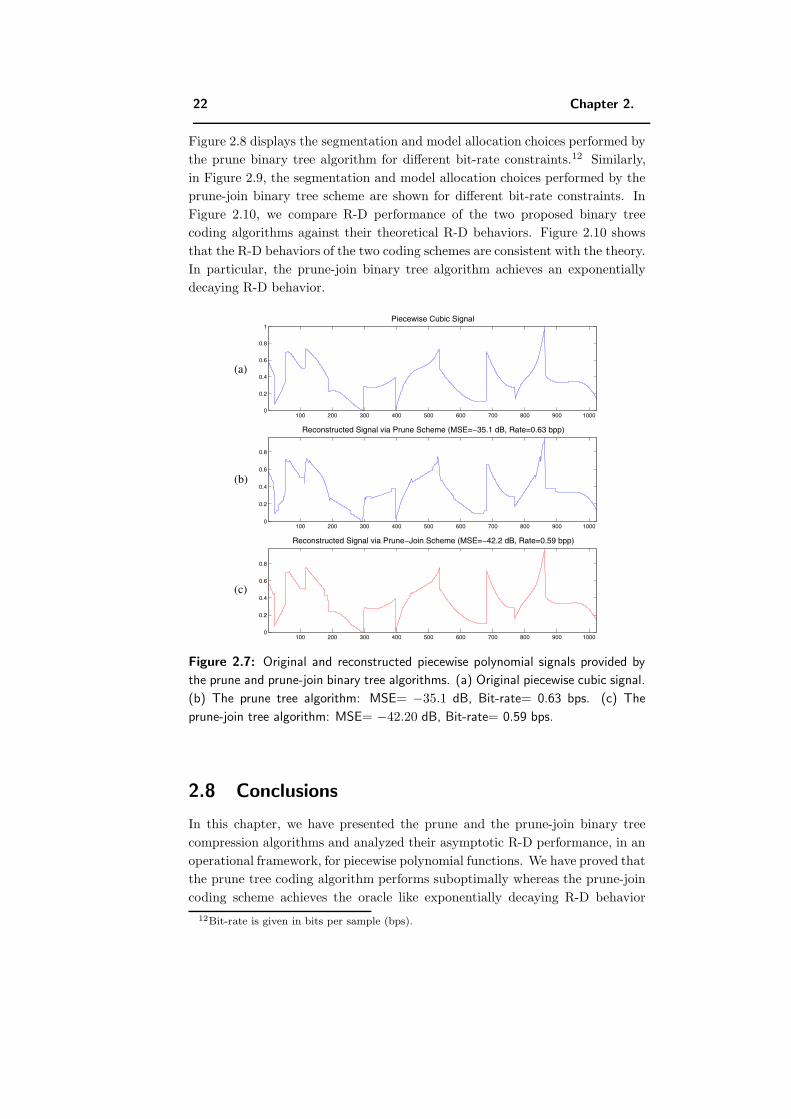
Figure 2.7 shows a particular realization of the piecewise cubic signal along
with reconstructed signals by the prune and the prune-join binary tree schemes.
22 Chapter 2.
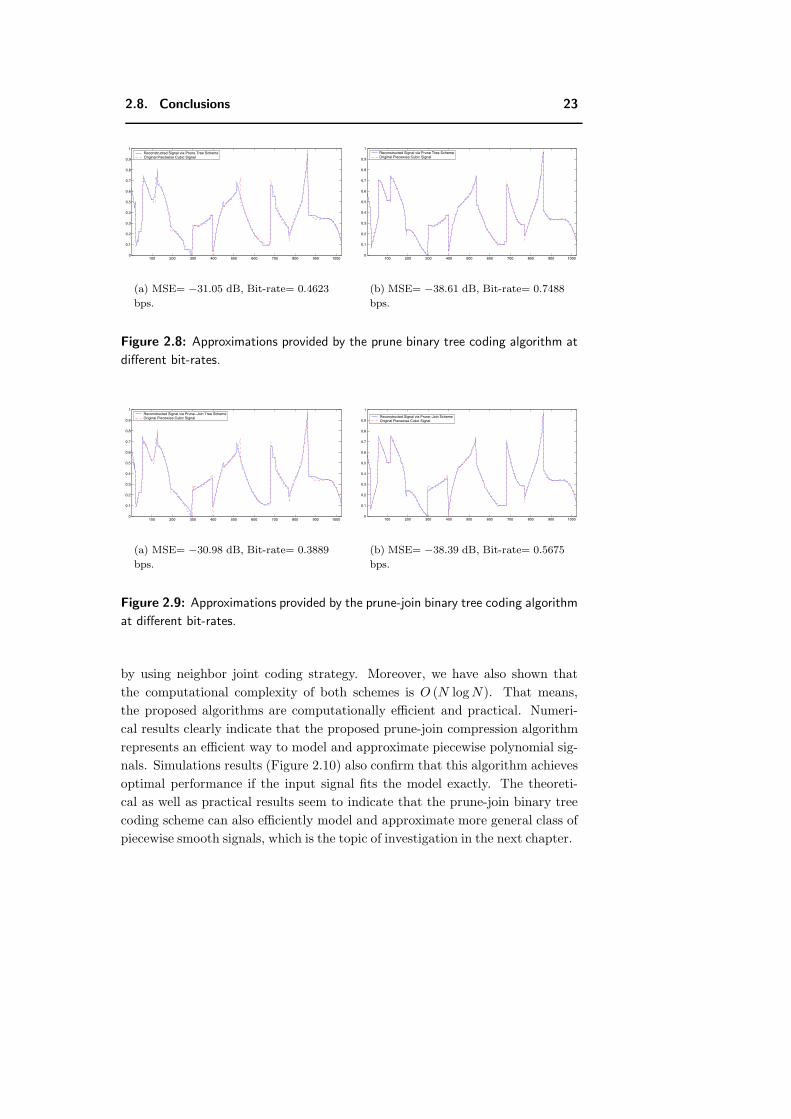
Figure 2.8 displays the segmentation and model allocation choices performed by
the prune binary tree algorithm for different bit-rate constraints.12 Similarly,
in Figure 2.9, the segmentation and model allocation choices performed by the
prune-join binary tree scheme are shown for different bit-rate constraints. In
Figure 2.10, we compare R-D performance of the two proposed binary tree
coding algorithms against their theoretical R-D behaviors. Figure 2.10 shows
that the R-D behaviors of the two coding schemes are consistent with the theory.
In particular, the prune-join binary tree algorithm achieves an exponentially
decaying R-D behavior.
100 200 300 400 500 600 700 800 900 10000
0.2
0.4
0.6
0.8
Reconstructed Signal via Prune Scheme (MSE=−35.1 dB, Rate=0.63 bpp)
100 200 300 400 500 600 700 800 900 10000
0.2
0.4
0.6
0.8
Reconstructed Signal via Prune−Join Scheme (MSE=−42.2 dB, Rate=0.59 bpp)
100 200 300 400 500 600 700 800 900 10000
0.2
0.4
0.6
0.8
1Piecewise Cubic Signal
(a)
(b)
(c)
Figure 2.7: Original and reconstructed piecewise polynomial signals provided by
the prune and prune-join binary tree algorithms. (a) Original piecewise cubic signal.
(b) The prune tree algorithm: MSE= −35.1 dB, Bit-rate= 0.63 bps. (c) The
prune-join tree algorithm: MSE= −42.20 dB, Bit-rate= 0.59 bps.
2.8 Conclusions
In this chapter, we have presented the prune and the prune-join binary tree
compression algorithms and analyzed their asymptotic R-D performance, in an
operational framework, for piecewise polynomial functions. We have proved that
the prune tree coding algorithm performs suboptimally whereas the prune-join
coding scheme achieves the oracle like exponentially decaying R-D behavior
12Bit-rate is given in bits per sample (bps).
2.8. Conclusions 23
100 200 300 400 500 600 700 800 900 10000
0.1
0.2
0.3
0.4
0.5
0.6
0.7
0.8
0.9
1Reconstructed Signal via Prune Tree SchemeOriginal Piecewise Cubic Signal
(a) MSE= −31.05 dB, Bit-rate= 0.4623
bps.
100 200 300 400 500 600 700 800 900 10000
0.1
0.2
0.3
0.4
0.5
0.6
0.7
0.8
0.9
1Reconstructed Signal via Prune Tree SchemeOriginal Piecewise Cubic Signal
(b) MSE= −38.61 dB, Bit-rate= 0.7488
bps.
Figure 2.8: Approximations provided by the prune binary tree coding algorithm at
different bit-rates.
100 200 300 400 500 600 700 800 900 10000
0.1
0.2
0.3
0.4
0.5
0.6
0.7
0.8
0.9
1Reconstructed Signal via Prune−Join Tree SchemeOriginal Piecewise Cubic Signal
(a) MSE= −30.98 dB, Bit-rate= 0.3889
bps.
100 200 300 400 500 600 700 800 900 10000
0.1
0.2
0.3
0.4
0.5
0.6
0.7
0.8
0.9
1
Reconstructed Signal via Prune−Join SchemeOriginal Piecewise Cubic Signal
(b) MSE= −38.39 dB, Bit-rate= 0.5675
bps.
Figure 2.9: Approximations provided by the prune-join binary tree coding algorithm
at different bit-rates.
by using neighbor joint coding strategy. Moreover, we have also shown that
the computational complexity of both schemes is O (N log N). That means,
the proposed algorithms are computationally efficient and practical. Numeri-
cal results clearly indicate that the proposed prune-join compression algorithm
represents an efficient way to model and approximate piecewise polynomial sig-
nals. Simulations results (Figure 2.10) also confirm that this algorithm achieves
optimal performance if the input signal fits the model exactly. The theoreti-
cal as well as practical results seem to indicate that the prune-join binary tree
coding scheme can also efficiently model and approximate more general class of
piecewise smooth signals, which is the topic of investigation in the next chapter.
24 Chapter 2.
0 0.5 1 1.5 2 2.5 3 3.5 4 4.5 5−200
−150
−100
−50
0
50
Bit−Rate (bpp) M
SE
(dB
)
Pruned Binary treePruned Binary tree (Bound)Prune−Join Binary treePrune−Join Binary tree (Bound)
Figure 2.10: Theoretical (solid) and numerical (dotted) R-D curves for the prune
and prune-join binary tree algorithms for piecewise polynomial signals.
Appendix 2.A Proof of Lemma 2.1: Parent Children
Pruning
Assume that the parent node is representing a piecewise polynomial function
f (t), defined over the interval [0, T ], with polynomial pieces of maximum degree
P . Let p (t) be the best (least square error) polynomial approximation of f (t).
Hence, p (t) minimizes the approximation distortion
D∞ =
∫ T
0
(f(t) − p(t))2dt. (2.20)
Since p (t) minimizes the approximation distortion D∞, the error function
(f (t) − p (t)) must be orthogonal to any polynomial q (t) of degree P . That
means, ∫ T
0
(f (t) − p (t)) q (t) dt = 0. (2.21)
Clearly, D∞ = 0 if f (t) is simply a polynomial of maximum degree P ,
otherwise D∞ > 0. Suppose that the polynomial p (t) is further quantized to
p (t) according to the given bit budget R. As shown in [40],∫ T
0
(p (t) − p (t))2 dt ≤ A2T (P + 1)2 2−2
P+1 R. (2.22)
Therefore, the R-D function for the parent node can be written as follows
D (R) =
∫ T
0
(f(t) − p(t))2 =
∫ T
0
(f(t) − p(t) + p(t) − p(t))2
=
∫ T
0
(f (t) − p (t))2
+
∫ T
0
(p (t) − p (t))2; due to orthogonality by (2.21)
≤ D∞ + A2T (P + 1)2 2−2
P+1 R; from (2.20) and (2.22). (2.23)
2.A. Proof of Lemma 2.1: Parent Children Pruning 25
Again, it is obvious that if the function f (t) has no singularity, then D∞ =
0. Since we are interested in the asymptotic R-D behavior, we will simply
utilize the R-D bound given by (2.23) for further analysis. Thus, the asymptotic
Lagrangian cost bound L (λ) is
L (λ) = D∞ + A2T (P + 1)22−
2P+1 R + λR. (2.24)
The minimization of the Lagrangian bound results into the following rate
allocation
R =P + 1
2log2
(2A2T (P + 1) ln 2
λ
). (2.25)
Combining (2.24) and (2.25), the minimum Lagrangian cost becomes
L (λ) = D∞ +λ
2(P + 1) log2
(2A2T (P + 1) e ln 2
λ
). (2.26)
Similarly, the minimum Lagrangian costs for the children nodes are as follows
L1 (λ) = D1∞ +λ
2(P + 1) log2
(2A2T1 (P + 1) e ln 2
λ
)(2.27)
L2 (λ) = D2∞ +λ
2(P + 1) log2
(2A2T2 (P + 1) e ln 2
λ
), (2.28)
where D1∞ and D2∞ represent the polynomial approximation error for the first
and second segment at infinite rate, respectively and T1 = T2 = T2 . Thus, the
difference in the Lagrangian cost of the parent and that of its children can be
written as follows
∆L (λ) = L (λ) − L1 (λ) − L2 (λ)
= (D∞ − D1∞ − D2∞) +λ
2(P + 1) log2
(λT
2A2T1T2 (P + 1) e ln 2
).
If the signal has no singularity, then D∞ = D1∞ = D2∞ = 0. Therefore,
the difference in the Lagrangian costs becomes
∆L (λ) =λ
2(P + 1) log2
(λT
2A2T1T2 (P + 1) e ln 2
)∆L (λ) < 0; for λ < λ0 =
2
TA2T1T2 (P + 1) e ln 2. (2.29)
Clearly , at high rates, R ≥ 2, so λ ≤ 12A2T < λ0.
13 Thus, (2.29) ensures that
the Lagrangian cost of the parent is smaller than the sum of the Lagrangian
costs of its children if the parent has no singularity. Hence, the children are
pruned.
13For a rate of zero bits, the resulting distortion D0 is equal to the energy of the entire signal.
That means, D0 = A2T . Let λ be such that (R∗(λ), D∗(λ)) is optimum with R∗(λ) ≥ 2 bits.
Due to the R-D optimization, for all (R, D) pairs, D + λR ≥ D∗(λ) + λR∗(λ). Since this
relation is also true for (0, D0), the following holds : λ ≤ D0−D∗(λ)R∗(λ)
≤ 12A2T < λ0.
26 Chapter 2.
Similarly, if the signal has a singularity, then one can easily show that D∞−D1∞ − D2∞ > 0.14 Therefore, the difference in the Lagrangian costs becomes
∆L (λ) = (D∞ − D1∞ − D2∞) +λ
2(P + 1) log2
„λT
2A2T1T2 (P + 1) e ln 2
«= (D∞ − D1∞ − D2∞) ; as at high rates, λ → 0 and lim
λ→0λ log λ → 0
⇒ ∆L (λ) > 0. (2.30)
Hence, the Lagrangian cost of the parent is greater than the sum of the La-
grangian costs of its children and the algorithm decides to split the parent.
Therefore, (2.29) and (2.30) clearly show that the Lagrangian cost of the parent
is smaller than the sum of the Lagrangian costs of the children if and only if
the parent has no singularity. This implies that, at high rates, the children are
pruned if and only if the parent contains no singularity.
Appendix 2.B Proof of Lemma 2.3: Neighbor Join-
ing
In essence, the proof of Lemma 2.3 closely follows the logic outlined for the
proof of Lemma 2.1. Suppose that we have two neighboring blocks of size T1
and T2, then the joint block (node) will be of size T = (T1 + T2). This can
be interpreted as the segmentation of the joint block into the two segments of
size T1 and T2. Then (2.29) and (2.30) clearly show that the Lagrangian cost
of the joint node will be smaller than the sum of the Lagrangian costs of the
neighboring blocks if and only if the joint block has no singularity. Therefore,
at high rates, the neighboring nodes will be merged if and only if the joint block
contains no singularity.
14It is also intuitive as the segmentation provides the finer representation for the complete
signal.
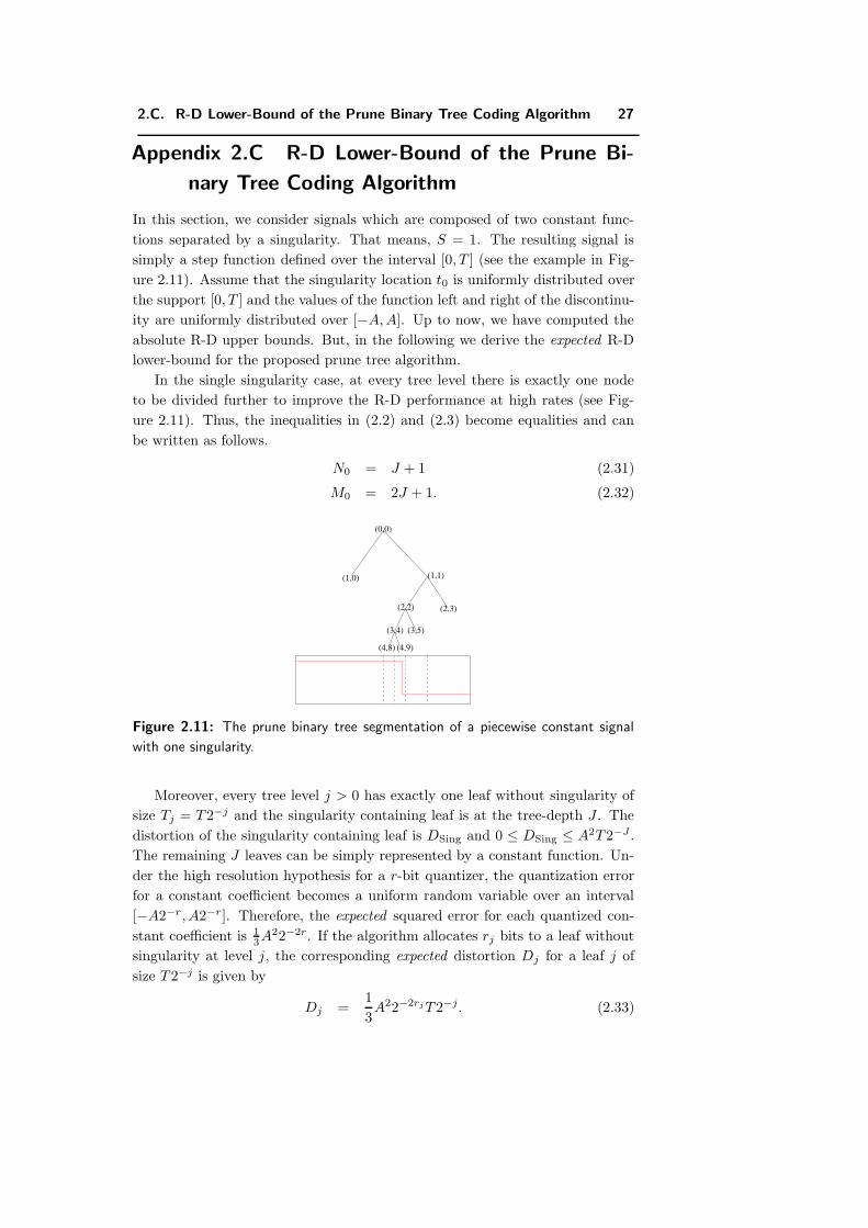
2.C. R-D Lower-Bound of the Prune Binary Tree Coding Algorithm 27
Appendix 2.C R-D Lower-Bound of the Prune Bi-
nary Tree Coding Algorithm
In this section, we consider signals which are composed of two constant func-
tions separated by a singularity. That means, S = 1. The resulting signal is
simply a step function defined over the interval [0, T ] (see the example in Fig-
ure 2.11). Assume that the singularity location t0 is uniformly distributed over
the support [0, T ] and the values of the function left and right of the discontinu-
ity are uniformly distributed over [−A, A]. Up to now, we have computed the
absolute R-D upper bounds. But, in the following we derive the expected R-D
lower-bound for the proposed prune tree algorithm.
In the single singularity case, at every tree level there is exactly one node
to be divided further to improve the R-D performance at high rates (see Fig-
ure 2.11). Thus, the inequalities in (2.2) and (2.3) become equalities and can
be written as follows.
N0 = J + 1 (2.31)
M0 = 2J + 1. (2.32)
(0,0)
(2,2)
(3,4) (3,5)
(2,3)
(1,1)
(4,9)(4,8)
(1,0)
Figure 2.11: The prune binary tree segmentation of a piecewise constant signal
with one singularity.
Moreover, every tree level j > 0 has exactly one leaf without singularity of
size Tj = T 2−j and the singularity containing leaf is at the tree-depth J . The
distortion of the singularity containing leaf is DSing and 0 ≤ DSing ≤ A2T 2−J .
The remaining J leaves can be simply represented by a constant function. Un-
der the high resolution hypothesis for a r-bit quantizer, the quantization error
for a constant coefficient becomes a uniform random variable over an interval
[−A2−r, A2−r]. Therefore, the expected squared error for each quantized con-
stant coefficient is 13A22−2r. If the algorithm allocates rj bits to a leaf without
singularity at level j, the corresponding expected distortion Dj for a leaf j of
size T 2−j is given by
Dj =1
3A22−2rj T 2−j. (2.33)
28 Chapter 2.
Therefore, the overall expected distortion for the prune tree algorithm can
be written as follows
DP =
J∑j=1
Dj + DSing (2.34)
DP ≥J∑
j=1
1
3A2T 2−j2−2rj ; as DSing ≥ 0. (2.35)
Since the cost of coding the pruned binary tree is RTree = M0 = 2J + 1, the
net rate becomes
R =
J∑j=1
rj + RTree
R =
J∑j=1
rj + 2J + 1. (2.36)
Our goal is to find r1, r2, . . . , rJ and J such that the following Lagrangian
cost functional L(λ) is minimized15
L(λ) =
J∑j=1
1
3A2T 2−j2−2rj + λ
J∑j=1
rj + 2J + 1
. (2.37)
That means,
∂L
∂rj= 0, ∀j = 1, · · · , J
⇒ 1
3A2T 2−j2−2rj =
λ
2 ln 2; equal distortion constraint (2.38)
⇒ rj = rk +k − j
2; similar to (2.6)
⇒ rj = r1 +1 − j
2. (2.39)
By combining (2.37), (2.38) and (2.39), the Lagrangian cost functional can
be rewritten as follows
L(λ) = Jλ
2 ln 2+ λ
(Jr1 − J(J − 1)
4+ 2J + 1
). (2.40)
And
∂L
∂J= 0
⇒ λ
2 ln 2+ λ
(r1 − 2J − 1
4+ 2
)= 0
⇒ r1 =2J − 1
4− 2 − 1
2 ln 2. (2.41)
15This R-D bound based Lagrangian cost functional is obtained by combining the right
hand sides of (2.35) and (2.36).
2.C. R-D Lower-Bound of the Prune Binary Tree Coding Algorithm 29
Now, by combining (2.36) and (2.39), the total rate can be rewritten as
follows
R = Jr1 − J(J − 1)
4+ 2J + 1
= J
(2J − 1
4− 2 − 1
2 ln 2
)− J(J − 1)
4+ 2J + 1; from (2.41)
⇒ R ≥ 1
4(J − 2)2. (2.42)
From (2.38), it is also clear that
1
3A2T 2−12−2r1 =
λ
2 ln 2. (2.43)
Combining (2.41) and (2.43), we obtain
16e
3A2T 2−J =
λ
2 ln 2. (2.44)
By combining (2.35), (2.38) and (2.44), we obtain the following R-D lower-
bound
DP ≥ J16e
3A2T 2−J (2.45)
DP ≥ 8e
3A2T
(√R + 1
)2−2
√R; combining (2.42) and (2.45).
⇒ DP ≥ 8e
3A2T
√R2−2
√R
The above result is summarized in the following theorem.
Theorem 2.3 The prune binary tree coding algorithm, which employs the
bottom-up R-D optimization using parent-children pruning, achieves an asymp-
totic R-D behavior which is lower bounded (in expectation) as follows
DP (R) ≥ c′2√
R2−c′3√
R, (2.46)
where c′2 = 8e3 A2T and c′3 = 2, for piecewise constant signals with only one
singularity.
Theorem 2.3 also indicates that, on average, the prune binary tree algorithm
will necessarily perform worse than (2.46) for more general piecewise polynomial
signals with multiple singularities. Therefore, on average, the prune binary tree
coding algorithm performs suboptimally.
Since the prune-join tree algorithm already achieves the oracle like expo-
nentially decaying R-D behavior (Theorem 2.2) , computation of its R-D lower-
bound will not provide any interesting information. That is why the lower-bound
analysis is not presented for the prune-join tree algorithm.

30 Chapter 2.
Chapter 3
Binary Tree Segmentation
Algorithms and 1-D Piecewise
Smooth Signals
3.1 Introduction
It is intuitive that many signals encountered in practice can be closely modeled
as piecewise smooth. Thus, if a coding scheme can accurately represent piece-
wise smooth signals, it might have an important impact on signal processing
applications like approximation and compression of real life signals. That is
why, in this chapter, we study whether the proposed binary tree segmentation
algorithms can accurately model piecewise smooth signals. In the chapter, our
main focus is on the tree segmentation based polynomial approximation of 1-D
piecewise smooth signals. In the next section, we analyze the R-D performance
of the binary tree algorithms for 1-D smooth signals. We then extend this R-D
analysis to the more general piecewise smooth signals in Section 3.3. In particu-
lar, we show that both the prune and prune-join tree schemes are able to achieve
the oracle like R-D behavior. In Section 3.4, we present experimental results
which are also consistent with the theoretical analysis. Finally, Section 3.5 offers
concluding remarks.
3.2 R-D Analysis for 1-D Smooth Functions
Our interest is in piecewise smooth signals, which are composed of regular pieces.
The regularity of a function is generally measured by the Holder exponent [32,
33].
31
32 Chapter 3.
Definition 3.1
• A function f(t) is pointwise Holder α ≥ 0 at t0, if there exist a K > 0,
and a polynomial pt0(t) of degree P = α such that1
∀t ∈ R, |f(t) − pt0(t)| ≤ K|t − t0|α. (3.1)
• A function f(t) is uniformly Holder α over [a, b] if it satisfies (3.1) for all
t0 ∈ [a, b], with a constant K that is independent of t0.
• The Holder regularity of f(t) at t0 or over [a, b] is the supremum of the α
such that f(t) is Holder α.
Moreover, for a uniformly Holder α smooth function f(t), the polynomial
pt0(t), in (3.1), is the P th order Taylor series expansion of f(t) around the point
t0. Since the regularity of a function guarantees that the function can be well
approximated by an appropriate polynomial, our aim is to investigate whether
the binary tree segmentation based coding algorithm, which utilizes this fact,
can achieve the correct R-D performance.
3.2.1 R-D Performance of the Oracle Method
Consider a continuous-time smooth signal f(t), which is uniformly Holder α
regular according to Definition 3.1. For such a signal, it has been shown in [9]
that the best asymptotic R-D upper-bound is as follows
D(R) ≤ CR−2α, (3.2)
for some constant C > 0.
3.2.2 R-D Analysis of the Binary Tree Algorithms
Theorem 3.1 For 1-D smooth functions, which are uniformly Holder α over
[0, T ], the full binary tree decomposition algorithm, which codes every binary tree
node at the tree depth by a polynomial approximation, achieves the following
asymptotic R-D behavior
DFull (R) ≤ d0
(log R
R
)2α
, (3.3)
where d0 is a positive constant which depends on the smoothness, magnitude and
region of support of the function.
Proof: Consider a 1-D function f(t), which is uniformly Holder α smooth and
defined over the region [0, T ]. The binary tree decomposition leads to the dyadic
intervals of size T 2−J at the depth J . These intervals can be represented by
1To be more precise, α and P are such that P < α ≤ P + 1.
3.2. R-D Analysis for 1-D Smooth Functions 33
Ri = [i, (i + 1)]T 2−J ; 0 ≤ i < 2J . The binary tree algorithm approximates
the function in each segment Ri by its best (least square error) polynomial
approximation pi(t) of degree P = α. Since pi(t) is the best P th order poly-
nomial approximation of the function f(t) on the region Ri, f(t)− pi(t) will be
orthogonal to any P th order polynomial q(t) on the region Ri. That means,
∫Ri
(f(t) − pi(t))) q(t) = 0. (3.4)
Due to (3.1), the polynomial approximation squared error for the region Ri can
be bounded as follows
∫Ri
(f(t) − pi(t))2 ≤
∫Ri
K2i |t − xi|2α
≤ K2i
∫Ri
(T 2−J)2α
≤ K2maxT
2α2−2αJT 2−J
= K02−2αJT 2−J ; K0 = K2
maxT2α, (3.5)
where xi is the origin coordinate of the tree node associated with region Ri and
Kmax = max0≤i<2J Ki.
The binary tree algorithm codes the polynomial pi(t) by quantizing its (P+1)
coefficients. Assume that the algorithm allocates ri bits to the polynomial pi(t).
Suppose that the polynomials pi(t), i = 0, . . . , 2J −1, are bounded in magnitude
by some constant A. Thus, the polynomial quantization distortion di for the
region Ri due to the coefficient quantization can be bounded as follows [40]
di =
∫Ri
(pi(t) − pi(t))2
≤ A20T 2−J2−
2P+1 ri ; A0 = A(P + 1). (3.6)
Hence, the coding distortion Di for the region Ri is as follows
Di =
∫Ri
(f(t) − pi(t))2
=
∫Ri
(f(t) − pi(t) + pi(t) − pi(t))2
=
∫Ri
(f(t) − pi(t))2 +
∫Ri
(pi(t) − pi(t))2 , due to (3.4)
≤ K02−2αJT 2−J + A2
0T 2−J2−2
P+1 ri , from (3.5) and (3.6). (3.7)
The binary tree scheme provides the piecewise polynomial approximation p(t) =∑2J−1i=0 pi1Ri
(t), which is further quantized to p(t) =∑2J−1
i=0 pi(t)1Ri(t). There-
34 Chapter 3.
fore, the overall coding distortion can be written as follows
D =
∫[0,T ]
(f(t) − p(t))2
=
2J−1∑i=0
∫Ri
(f(t) − pi(t))2
≤2J−1∑i=0
[K02
−2αJT 2−J + A20T 2−J2−
2P+1 ri
], from (3.7)
= K0T 2−2αJ +
2J−1∑i=0
A20T 2−J2−
2P+1 ri . (3.8)
The structure of (3.8) ensures that R-D optimization results in the equal dis-
tortion for all the leaves.2 That means, all the leaves will be allocated the same
rate, i.e. ri = r, ∀i = 0, . . . , 2J − 1. Moreover, we can notice from (3.7) that the
distortion of a leaf is the sum of two terms and the best R-D performance for
a leaf will be achieved when both terms are of the same order.3 Hence, for the
given bit-budget R, the algorithm selects J and r such that the distortion of
each leaf is of the order O(2−2αJ−J ). Thus, the scheme allocates r = (P +1)αJ
bits to each polynomial associated with a leaf. Therefore, the net distortion can
be expressed as follows
D ≤ (K0 + A20)T 2−2αJ
= K12−2αJ ; K1 = (K0 + A2
0)T
≤ K1
(1 +
log J
J
)2α
2−2αJ , as at high rates J > 1. (3.9)
Since the full binary tree decomposition algorithm does not need to code the
tree structure, the global bit budget is simply equal to the total bits required
for quantizing the polynomial coefficients associated with 2J binary tree leaves
at the tree depth J . Hence, the net rate is as follows
R = 2Jr = 2J(P + 1)αJ
R = K2J2J ; K2 = (P + 1)α,
log2
(R
K2
)= log2 J + J. (3.10)
2This result can be derived using the usual reverse water filling technique. That is, ∂D∂ri
=
constant.3Because if both terms are not of the same order, then one of the terms will dominate the
overall distortion and the R-D performance can be improved by reselecting J and r.
3.2. R-D Analysis for 1-D Smooth Functions 35
Combining (3.9) and (3.10) leads to the following asymptotic R-D behavior
D ≤ K1
log2
(RK2
)RK2
2α
≤ K1K2α2
(K2 + 1
K2
)log R
R
2α
, as at high rates R > 2
D ≤ d0
(log R
R
)2α
, (3.11)
where d0 = K1
(K2
2 + 1)2α
=(K2
maxT2α + A2
0
)T((P + 1)2α2 + 1
)2α.
Corollary 3.1 The prune binary tree coding algorithm achieves the following
asymptotic R-D behavior
DPrune (R) ≤ d0
(log R
R
)2α
, (3.12)
for 1-D smooth functions, which are uniformly Holder α over [0, T ].
Proof: Since the prune binary tree algorithm results into the full binary tree
algorithm, when no pruning is performed, the prune binary tree scheme will
perform at least as well as the full tree scheme. Thus, the prune tree scheme
will also achieve the R-D behavior given by (3.12).
Corollary 3.2 The prune-join binary tree algorithm achieves the following
asymptotic R-D behavior
DPrune-Join ≤ d0
(log R
R
)2α
, (3.13)
for 1-D smooth functions, which are uniformly Holder α over [0, T ].
Proof: Since the prune-join binary tree algorithm leads to the full binary tree
algorithm, when pruning and neighbor joining are not performed, the prune-
join tree scheme will perform at least as well as the full tree scheme. Thus, the
prune-join tree scheme will also achieve the R-D behavior shown by (3.13).
Therefore, for uniformly Holder α smooth 1-D functions, the full, the
prune and the prune-join schemes achieve the similar asymptotic R-D behavior(d0
(log R
R
)2α)
. However, note that the given R-D bound is a weak upper-
bound for both the prune and the prune-join coding schemes.
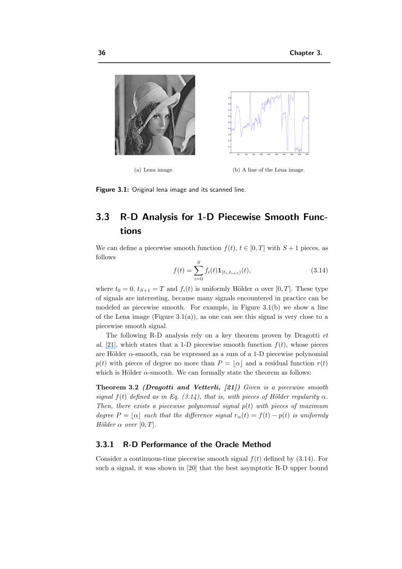
36 Chapter 3.
(a) Lena image.
50 100 150 200 250 300 350 400 450 5000
0.1
0.2
0.3
0.4
0.5
0.6
0.7
0.8
0.9
(b) A line of the Lena image.
Figure 3.1: Original lena image and its scanned line.
3.3 R-D Analysis for 1-D Piecewise Smooth Func-
tions
We can define a piecewise smooth function f(t), t ∈ [0, T ] with S + 1 pieces, as
follows
f(t) =S∑
i=0
fi(t)1[ti,ti+1)(t), (3.14)
where t0 = 0, tS+1 = T and fi(t) is uniformly Holder α over [0, T ]. These type
of signals are interesting, because many signals encountered in practice can be
modeled as piecewise smooth. For example, in Figure 3.1(b) we show a line
of the Lena image (Figure 3.1(a)), as one can see this signal is very close to a
piecewise smooth signal.
The following R-D analysis rely on a key theorem proven by Dragotti et
al. [21], which states that a 1-D piecewise smooth function f(t), whose pieces
are Holder α-smooth, can be expressed as a sum of a 1-D piecewise polynomial
p(t) with pieces of degree no more than P = α and a residual function r(t)
which is Holder α-smooth. We can formally state the theorem as follows:
Theorem 3.2 (Dragotti and Vetterli, [21]) Given is a piecewise smooth
signal f(t) defined as in Eq. (3.14), that is, with pieces of Holder regularity α.
Then, there exists a piecewise polynomial signal p(t) with pieces of maximum
degree P = α such that the difference signal rα(t) = f(t) − p(t) is uniformly
Holder α over [0, T ].
3.3.1 R-D Performance of the Oracle Method
Consider a continuous-time piecewise smooth signal f(t) defined by (3.14). For
such a signal, it was shown in [20] that the best asymptotic R-D upper bound
3.3. R-D Analysis for 1-D Piecewise Smooth Functions 37
is as follows
D(R) ≤ CR−2αs + d12
−d2Rp , (3.15)
where R = Rs + Rp; Rs and Rp are bitrates used to code the smooth residual
and the piecewise polynomial signal, respectively.
3.3.2 R-D Analysis of the Binary Tree Algorithms
Theorem 3.3 For 1-D piecewise smooth functions with uniformly Holder α
smooth pieces, the prune binary tree algorithm, which employs the parent-
children pruning, achieves the following asymptotic R-D behavior
DPrune (R) ≤ d3
(log R
R
)2α
, (3.16)
where d3 is a positive constant which depends on the characteristics, like number
of smooth pieces and their smoothness, of piecewise smooth functions.
Proof: The following asymptotic R-D analysis utilizes the insights gained from
the analysis of piecewise polynomial signals (Section 2.4) and that of smooth
functions (Section 3.2.2). From Section 2.4, we learn that the R-D optimiza-
tion performs finer segmentation in the singularity containing regions4 and also
selects a bit allocation strategy to ensure that all the tree leaves have the distor-
tion of the same order. On the other hand, Section 3.2.2 tells us that a smooth
function can be well represented by segmentation and corresponding piecewise
polynomial approximation.
Assume that the 1-D piecewise smooth function f(t), as defined in (3.14), is
decomposed using binary tree algorithm up to the tree depth J . Since the signal
contains only S singularities, each tree level j can have at most S singularity
containing nodes and the remaining 2j − S nodes can be simply represented by
smooth functions. Clearly, at high rates, for achieving better R-D performance
the tree pruning scheme will decompose the nodes with singular points deeper
compared to nodes without singularities (smooth nodes). Suppose that the
prune tree algorithm splits smooth nodes only up to the tree level J1 and beyond
this level only singularity containing nodes are further splitted.5 Since the prune
tree scheme can split at most S singularity containing nodes beyond the tree
level J1, every level beyond J1, except j = J , will generate at most S leaves.
The level J will have 2S leaves, while the level J1 will have 2J1 −S leaves. Thus,
the total number N0 of leaves can be bounded as follows
N0 ≤ (2J1 − S
)+ 2S + (J − 1 − J1)S = 2J1 + (J − J1)S. (3.17)
Moreover, it can also be noted that in the pruned tree, every tree level j > J1
can have at most 2S nodes. Hence, the total number M0 of nodes in the pruned
4Because polynomials cannot model segments with singularities.5This means that there is no leaf up to the tree level J1 − 1.
38 Chapter 3.
tree can be given as follows
M0 ≤ 2 · 2J1 + 2S (J − J1) . (3.18)
Clearly, in the worst case scenario, all the singularity containing leaves will
be at the tree depth J , so the size of each of them will be T 2−J . The distortion of
each of these leaves can be bounded by A2T 2−J .6 We can notice from (3.7) that
the distortion of a smooth leaf l at tree level j is bounded by K02−2αjT 2−j +
A20T 2−j2−
2P+1 rl , where rl is the rate allocated to the smooth leaf. Again, R-
D optimization requires that all the tree leaves must have the distortion of the
same order. Thus, the algorithm selects J = (2α+1)J1 and allocates (P +1)αJ1
bits to each polynomial associated with a smooth leaf. This ensures that all the
leaves have distortions of similar order O(2−(2α+1)J1
). Therefore, the total
distortion can be bounded as follows
D ≤ N0
(K0 + A2
0
)T 2−J12−2αJ1
≤ (2J1 + 2αJ1S
) (K0 + A2
0
)T 2−J12−2αJ1 , from (3.17)
≤ (2αS + 1)2J1(K0 + A2
0
)T 2−J12−2αJ1
= K12−2αJ1 ; K1 = (2αS + 1)
(K0 + A2
0
)T. (3.19)
The total bitrate is the sum of the costs of coding the tree structure and the
quantized model parameters of the smooth leaves. The bitrate RTree required to
code the tree structure is equal to the total number M0 of nodes in the pruned
tree. Thus, (3.18) gives RTree ≤ 2 · 2J1 + 4αSJ1 ≤ 2(2αS + 1)2J1 . Since the
algorithm allocates (P + 1)αJ1 bits to leaves without singularities and zero bits
to leaves with singularities, the bitrate RLeaves needed for coding the leaves is
bounded as follows: RLeaves ≤ N0(P +1)αJ1 ≤ (2αS +1)(P +1)αJ12J1. Hence,
the total bit rate can be expressed as follows
R = RTree + RLeaves
≤ 2(2αS + 1)2J1 + (2αS + 1)(P + 1)αJ12J1
≤ (2αS + 1)((P + 1)α + 2)J12J1 ; as at high rates J1 ≥ 1
⇒ R ≤ K2J12J1; K2 = (2αS + 1)((P + 1)α + 2). (3.20)
Combining (3.19) and (3.20) provides the following asymptotic R-D behavior
D ≤ d3
(log R
R
)2α
, (3.21)
where d0 = K1K2α2 = (2αS + 1)
(K0 + A2
0
)T (2αS + 1)2α((P + 1)α + 2)2α.
Therefore, the prune binary tree algorithm achieves the announced R-D behav-
ior.
6Recall that the algorithm approximates leaves with singularities by the zero polynomial.
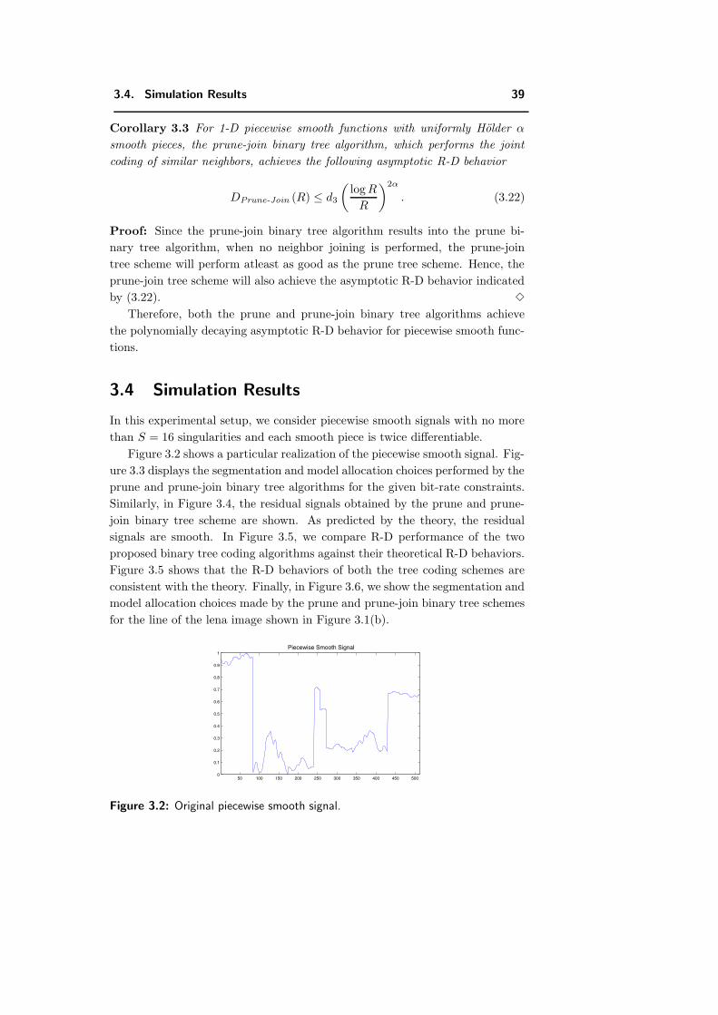
3.4. Simulation Results 39
Corollary 3.3 For 1-D piecewise smooth functions with uniformly Holder α
smooth pieces, the prune-join binary tree algorithm, which performs the joint
coding of similar neighbors, achieves the following asymptotic R-D behavior
DPrune-Join (R) ≤ d3
(log R
R
)2α
. (3.22)
Proof: Since the prune-join binary tree algorithm results into the prune bi-
nary tree algorithm, when no neighbor joining is performed, the prune-join
tree scheme will perform atleast as good as the prune tree scheme. Hence, the
prune-join tree scheme will also achieve the asymptotic R-D behavior indicated
by (3.22).
Therefore, both the prune and prune-join binary tree algorithms achieve
the polynomially decaying asymptotic R-D behavior for piecewise smooth func-
tions.
3.4 Simulation Results
In this experimental setup, we consider piecewise smooth signals with no more
than S = 16 singularities and each smooth piece is twice differentiable.
Figure 3.2 shows a particular realization of the piecewise smooth signal. Fig-
ure 3.3 displays the segmentation and model allocation choices performed by the
prune and prune-join binary tree algorithms for the given bit-rate constraints.
Similarly, in Figure 3.4, the residual signals obtained by the prune and prune-
join binary tree scheme are shown. As predicted by the theory, the residual
signals are smooth. In Figure 3.5, we compare R-D performance of the two
proposed binary tree coding algorithms against their theoretical R-D behaviors.
Figure 3.5 shows that the R-D behaviors of both the tree coding schemes are
consistent with the theory. Finally, in Figure 3.6, we show the segmentation and
model allocation choices made by the prune and prune-join binary tree schemes
for the line of the lena image shown in Figure 3.1(b).
50 100 150 200 250 300 350 400 450 5000
0.1
0.2
0.3
0.4
0.5
0.6
0.7
0.8
0.9
1 Piecewise Smooth Signal
Figure 3.2: Original piecewise smooth signal.
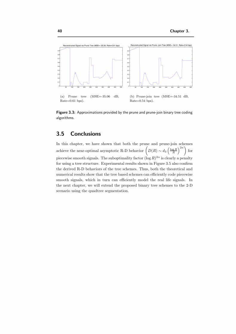
40 Chapter 3.
50 100 150 200 250 300 350 400 450 5000
0.1
0.2
0.3
0.4
0.5
0.6
0.7
0.8
0.9
Reconstructed Signal via Prune Tree (MSE=−35.06, Rate=0.61 bpp)
(a) Prune tree (MSE=-35.06 dB,
Rate=0.61 bps).
50 100 150 200 250 300 350 400 450 5000
0.1
0.2
0.3
0.4
0.5
0.6
0.7
0.8
0.9
1 Reconstructed Signal via Prune−Join Tree (MSE=−34.51, Rate=0.54 bpp)
(b) Prune-join tree (MSE=-34.51 dB,
Rate=0.54 bps).
Figure 3.3: Approximations provided by the prune and prune-join binary tree coding
algorithms.
3.5 Conclusions
In this chapter, we have shown that both the prune and prune-join schemes
achieve the near-optimal asymptotic R-D behavior
(D(R) ∼ d3
(log R
R
)2α)
for
piecewise smooth signals. The suboptimality factor (log R)2α is clearly a penalty
for using a tree structure. Experimental results shown in Figure 3.5 also confirm
the derived R-D behaviors of the tree schemes. Thus, both the theoretical and
numerical results show that the tree based schemes can efficiently code piecewise
smooth signals, which in turn can efficiently model the real life signals. In
the next chapter, we will extend the proposed binary tree schemes to the 2-D
scenario using the quadtree segmentation.
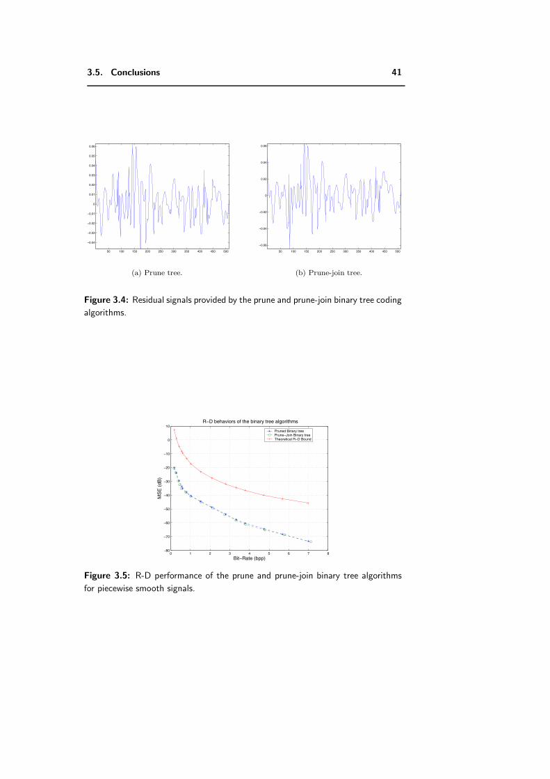
3.5. Conclusions 41
50 100 150 200 250 300 350 400 450 500
−0.04
−0.03
−0.02
−0.01
0
0.01
0.02
0.03
0.04
0.05
0.06
(a) Prune tree.
50 100 150 200 250 300 350 400 450 500
−0.06
−0.04
−0.02
0
0.02
0.04
0.06
(b) Prune-join tree.
Figure 3.4: Residual signals provided by the prune and prune-join binary tree coding
algorithms.
0 1 2 3 4 5 6 7 8−80
−70
−60
−50
−40
−30
−20
−10
0
10
Bit−Rate (bpp)
MS
E (
dB)
R−D behaviors of the binary tree algorithms
Pruned Binary treePrune−Join Binary treeTheoretical R−D Bound
Figure 3.5: R-D performance of the prune and prune-join binary tree algorithms
for piecewise smooth signals.
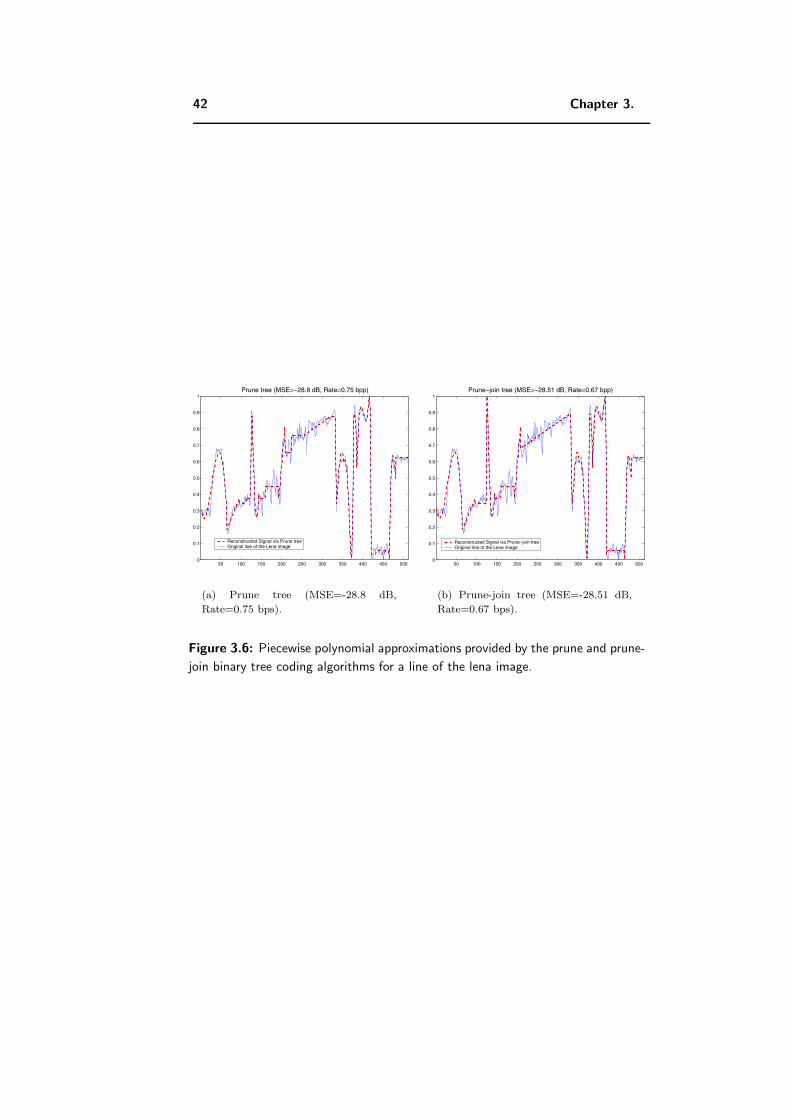
42 Chapter 3.
50 100 150 200 250 300 350 400 450 5000
0.1
0.2
0.3
0.4
0.5
0.6
0.7
0.8
0.9
1Prune tree (MSE=−28.8 dB, Rate=0.75 bpp)
Reconstructed Signal via Prune treeOriginal line of the Lena image
(a) Prune tree (MSE=-28.8 dB,
Rate=0.75 bps).
50 100 150 200 250 300 350 400 450 5000
0.1
0.2
0.3
0.4
0.5
0.6
0.7
0.8
0.9
1Prune−join tree (MSE=−28.51 dB, Rate=0.67 bpp)
Reconstructed Signal via Prune−join treeOriginal line of the Lena image
(b) Prune-join tree (MSE=-28.51 dB,
Rate=0.67 bps).
Figure 3.6: Piecewise polynomial approximations provided by the prune and prune-
join binary tree coding algorithms for a line of the lena image.
Chapter 4
Quadtree Segmentation
Algorithms and Piecewise
Polynomial Images
Although the situation is much more open and complex in two dimensions, it is
not hard to visualize the extension of the proposed 1-D coding scheme to the 2-D
case. Clearly, all the algorithms discussed so far in 1-D have an equivalent in 2-
D. The binary tree segmentation can be replaced by the quadtree segmentation
and polynomial model can be replaced by the 2-D geometrical model consisting
of two 2-D polynomials separated by a polynomial boundary. The Lagrangian
optimization algorithm remains the same. The neighbor joint coding algorithm
is more involved but it can be implemented efficiently. Therefore, we can have
an efficient quadtree based coding scheme for 2-D geometrical signals.
Note that in 1-D, the signal can contain only point-like singularities, which
can be efficiently captured by the binary tree segmentation. However, in 2-D,
the quadtree segmentation cannot capture the higher order edge singularities.1
Thus, we need to improve our node-model from simple polynomial to piecewise
polynomial with polynomial edge to capture the geometry inherent in the 2-D
images [16].
This chapter is organized as follows: Section 4.1 outlines the prune and
prune-join quadtree schemes. In Section 4.2, for the sake of simplicity, we
consider a simpler image model, which we call the polygonal model. In the
polygonal model, there is a white polygon shaped object against a uniform
black background (see Figure 4.1(a)). In Section 4.2.1, we present the oracle
R-D behavior. In Sections 4.2.2 and 4.2.3, we analyze the R-D performance
of the quadtree schemes. Similar to the 1-D case, we show that the prune-
join quadtree scheme achieves the oracle like asymptotic R-D behavior (The-
1As quadtree segmentation can model only horizontal and vertical edges at dyadic locations.
43
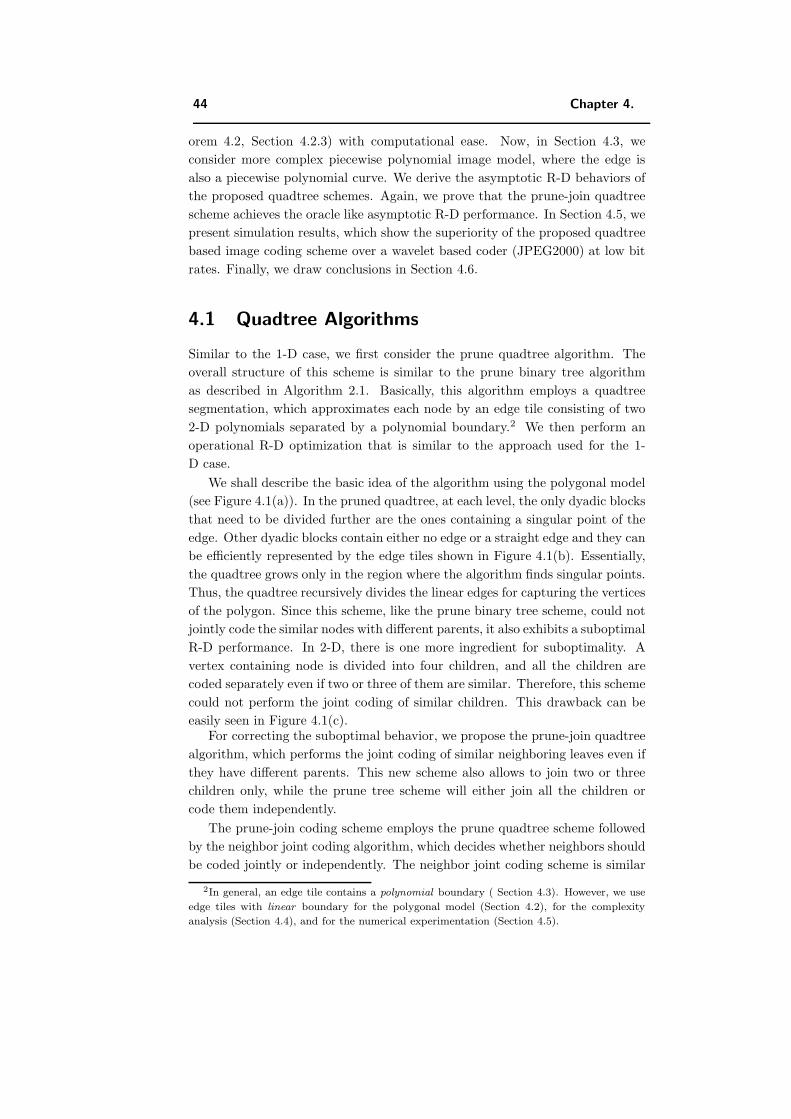
44 Chapter 4.
orem 4.2, Section 4.2.3) with computational ease. Now, in Section 4.3, we
consider more complex piecewise polynomial image model, where the edge is
also a piecewise polynomial curve. We derive the asymptotic R-D behaviors of
the proposed quadtree schemes. Again, we prove that the prune-join quadtree
scheme achieves the oracle like asymptotic R-D performance. In Section 4.5, we
present simulation results, which show the superiority of the proposed quadtree
based image coding scheme over a wavelet based coder (JPEG2000) at low bit
rates. Finally, we draw conclusions in Section 4.6.
4.1 Quadtree Algorithms
Similar to the 1-D case, we first consider the prune quadtree algorithm. The
overall structure of this scheme is similar to the prune binary tree algorithm
as described in Algorithm 2.1. Basically, this algorithm employs a quadtree
segmentation, which approximates each node by an edge tile consisting of two
2-D polynomials separated by a polynomial boundary.2 We then perform an
operational R-D optimization that is similar to the approach used for the 1-
D case.
We shall describe the basic idea of the algorithm using the polygonal model
(see Figure 4.1(a)). In the pruned quadtree, at each level, the only dyadic blocks
that need to be divided further are the ones containing a singular point of the
edge. Other dyadic blocks contain either no edge or a straight edge and they can
be efficiently represented by the edge tiles shown in Figure 4.1(b). Essentially,
the quadtree grows only in the region where the algorithm finds singular points.
Thus, the quadtree recursively divides the linear edges for capturing the vertices
of the polygon. Since this scheme, like the prune binary tree scheme, could not
jointly code the similar nodes with different parents, it also exhibits a suboptimal
R-D performance. In 2-D, there is one more ingredient for suboptimality. A
vertex containing node is divided into four children, and all the children are
coded separately even if two or three of them are similar. Therefore, this scheme
could not perform the joint coding of similar children. This drawback can be
easily seen in Figure 4.1(c).For correcting the suboptimal behavior, we propose the prune-join quadtree
algorithm, which performs the joint coding of similar neighboring leaves even if
they have different parents. This new scheme also allows to join two or three
children only, while the prune tree scheme will either join all the children or
code them independently.
The prune-join coding scheme employs the prune quadtree scheme followed
by the neighbor joint coding algorithm, which decides whether neighbors should
be coded jointly or independently. The neighbor joint coding scheme is similar
2In general, an edge tile contains a polynomial boundary ( Section 4.3). However, we use
edge tiles with linear boundary for the polygonal model (Section 4.2), for the complexity
analysis (Section 4.4), and for the numerical experimentation (Section 4.5).
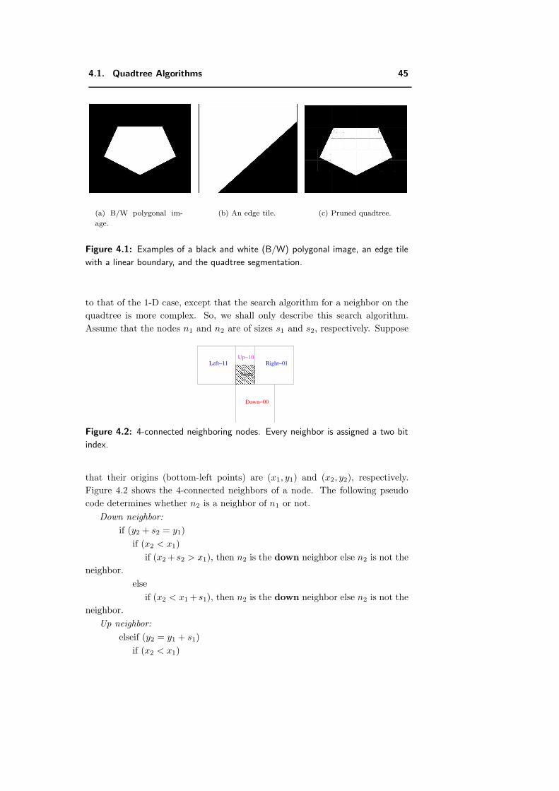
4.1. Quadtree Algorithms 45
(a) B/W polygonal im-
age.
(b) An edge tile. (c) Pruned quadtree.
Figure 4.1: Examples of a black and white (B/W) polygonal image, an edge tile
with a linear boundary, and the quadtree segmentation.
to that of the 1-D case, except that the search algorithm for a neighbor on the
quadtree is more complex. So, we shall only describe this search algorithm.
Assume that the nodes n1 and n2 are of sizes s1 and s2, respectively. Suppose
Right−01Up−10
Node
Down−00
Left−11
Figure 4.2: 4-connected neighboring nodes. Every neighbor is assigned a two bit
index.
that their origins (bottom-left points) are (x1, y1) and (x2, y2), respectively.
Figure 4.2 shows the 4-connected neighbors of a node. The following pseudo
code determines whether n2 is a neighbor of n1 or not.
Down neighbor:
if (y2 + s2 = y1)
if (x2 < x1)
if (x2 + s2 > x1), then n2 is the down neighbor else n2 is not the
neighbor.
else
if (x2 < x1 + s1), then n2 is the down neighbor else n2 is not the
neighbor.
Up neighbor:
elseif (y2 = y1 + s1)
if (x2 < x1)
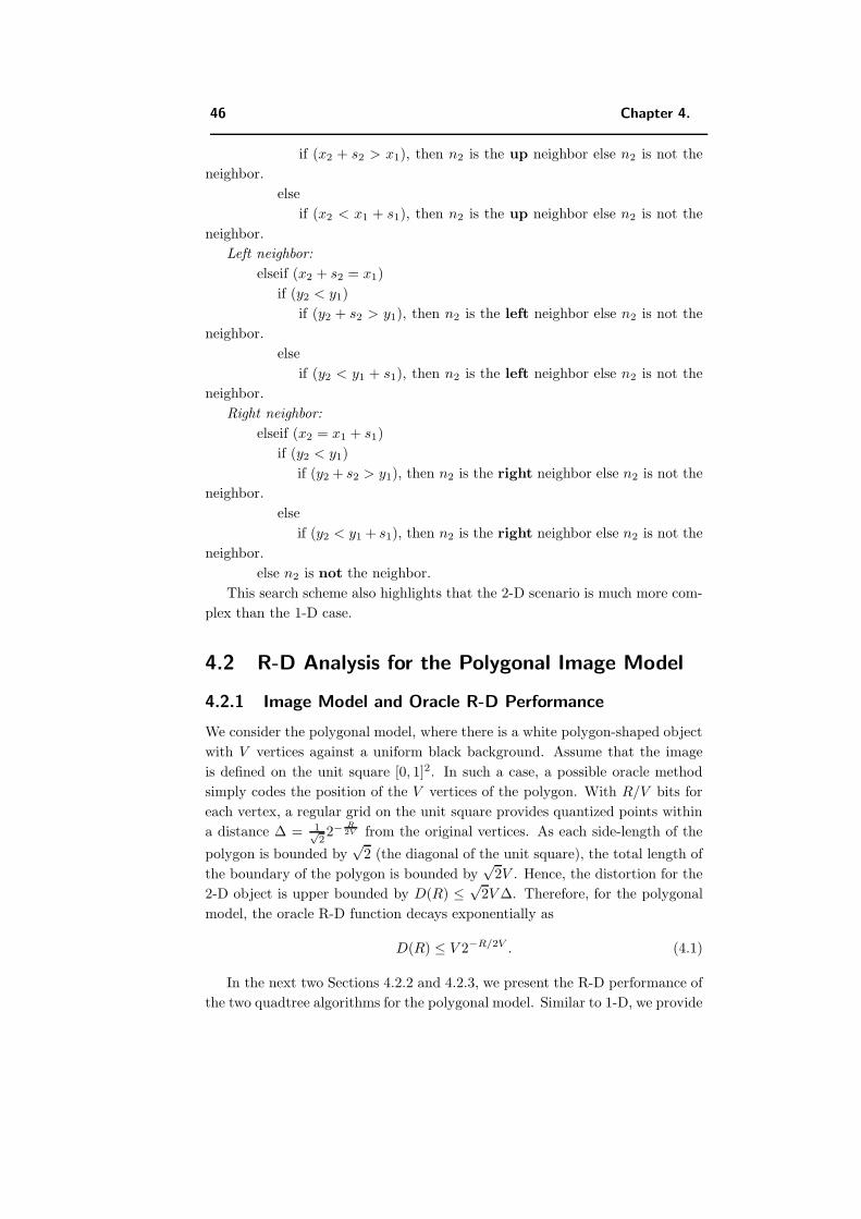
46 Chapter 4.
if (x2 + s2 > x1), then n2 is the up neighbor else n2 is not the
neighbor.
else
if (x2 < x1 + s1), then n2 is the up neighbor else n2 is not the
neighbor.
Left neighbor:
elseif (x2 + s2 = x1)
if (y2 < y1)
if (y2 + s2 > y1), then n2 is the left neighbor else n2 is not the
neighbor.
else
if (y2 < y1 + s1), then n2 is the left neighbor else n2 is not the
neighbor.
Right neighbor:
elseif (x2 = x1 + s1)
if (y2 < y1)
if (y2 + s2 > y1), then n2 is the right neighbor else n2 is not the
neighbor.
else
if (y2 < y1 + s1), then n2 is the right neighbor else n2 is not the
neighbor.
else n2 is not the neighbor.
This search scheme also highlights that the 2-D scenario is much more com-
plex than the 1-D case.
4.2 R-D Analysis for the Polygonal Image Model
4.2.1 Image Model and Oracle R-D Performance
We consider the polygonal model, where there is a white polygon-shaped object
with V vertices against a uniform black background. Assume that the image
is defined on the unit square [0, 1]2. In such a case, a possible oracle method
simply codes the position of the V vertices of the polygon. With R/V bits for
each vertex, a regular grid on the unit square provides quantized points within
a distance ∆ = 1√22−
R2V from the original vertices. As each side-length of the
polygon is bounded by√
2 (the diagonal of the unit square), the total length of
the boundary of the polygon is bounded by√
2V . Hence, the distortion for the
2-D object is upper bounded by D(R) ≤ √2V ∆. Therefore, for the polygonal
model, the oracle R-D function decays exponentially as
D(R) ≤ V 2−R/2V . (4.1)
In the next two Sections 4.2.2 and 4.2.3, we present the R-D performance of
the two quadtree algorithms for the polygonal model. Similar to 1-D, we provide
4.2. R-D Analysis for the Polygonal Image Model 47
only upper-bounds for operational R-D functions of the quadtree algorithms.
The reason is that this analysis provides us the insight into the R-D performance
of the algorithms in the high rate regime. Another reason is that it is difficult
to compute the exact R-D function in a general setting such as ours.
4.2.2 R-D Analysis of the Prune Quadtree Algorithm
Similar to the 1-D case, first we show that the prune quadtree scheme encodes
a number of leaves, which increases linearly with respect to the tree depth J .
We then present Theorem 4.1, which states the suboptimal R-D behavior of the
prune quadtree scheme.
Lemma 4.1 The prune quadtree coding algorithm will result in a quadtree with
a number of leaves upper-bounded by (3J + 1)V , where J and V represent the
decomposition depth of the tree and the number of vertices of the polygon in the
image, respectively.
Proof: Similar to the 1-D scenario, at high rates, the prune quadtree segmenta-
tion scheme recursively divides only those dyadic blocks which contain a vertex
of the polygon edge. Other dyadic blocks contain either no edge or a straight
edge, so they can be efficiently represented by the edge tiles with linear bound-
ary. Since the polygon has V vertices, there are at most V splitting nodes at
each tree level. Thus, they will generate no more than 3V leaves with a straight
edge at the next level. The leaves generated at depth J will be 4V , while the
level 0 cannot have any leaf at high rates for V > 0. Hence, the total number
N0 of leaves in the pruned quadtree is bounded as follows
N0 ≤ (J − 1)3V + 4V = (3J + 1)V. (4.2)
Similar to the 1-D case, every tree level can have at most 4V nodes. There-
fore, the total number M0 of nodes in the pruned quadtree can be given by
M0 ≤ 4JV + 1. (4.3)
The polygonal model image has a finite number of degrees of freedom, while
the prune quadtree scheme codes a number of parameters which grows linearly
with J . Therefore, it is bound to exhibit a suboptimal R-D behavior. This is
more formally enunciated in the following theorem.
Theorem 4.1 For the polygonal model, the prune quadtree coding algorithm,
which employs the parent-children pruning, results in the following asymptotic
R-D behavior
DP (R) ≤ c6
√R2−c7
√R, (4.4)
where c6 = 2√
6V and c7 =√
23V .
48 Chapter 4.
Proof: Since the polygonal image has V vertices, at most V leaves will have a
vertex. The remaining 3JV leaves (Lemma 4.1) can be simply represented by
edge tiles. If J is large enough, then in the worst case each vertex will lie in
a different dyadic square leaf at depth J . Their sizes will be 2−2J . Therefore,
the squared error distortion of each of the vertex containing leaves is bounded
by 142−2J , if the node is represented by the mean value 1
2 of the image dynamic
range (0, 1). The remaining leaves without vertices can be well approximated
by edge tiles. For coding an edge block with a linear-edge, we need to code
the locations of two vertices of the linear-edge on the boundary of the block.
The encoding order of these two vertices is simply used to specify the value of
the associated regions: for example, when one traverses from first vertex to the
second one, the black region is on the left. In particular, an edge leaf l at tree
level j is of side-length Tl = 2−j . In this case, if we allocate Rl
2 bits to each line-
vertex of the linear edge of the edge leaf, then the maximum distance between
the true line vertices and their quantized version is bounded by 2−j2−(Rl2 −1).
Thus, the distortion of an edge leaf will be bounded by 2−2j2−(Rl2 −1).3 Since
R-D optimal solution of exponentially decaying R-D functions results in equal
distortion for each leaf [12], the coding algorithm will allocate same rate Rj to
all the leaves without vertices at the same tree level j.
Similar to 1-D, R-D optimization results in a tree-depth J and a bit alloca-
tion strategy such that the edge leaves and the vertex containing leaves have a
distortion of the same order O(2−2J
). Therefore, the coding scheme will allo-
cate no bits to leaves with vertices and 2(2(J − j) + 1) bits to every edge block
at tree level j to ensure that the distortion for each leaf is bounded by 2−2J .
Since all the tree levels, except j = 0, can contribute 3V leaves with no vertex,
the total rate required for coding the leaves is
RLeaves = 3V
J∑j=1
2(2(J − j) + 1) = 6V J2. (4.5)
The tree split-merge decision variable will consume bits (RTree) equal to the
total number of nodes in the pruned tree. Thus, (4.3) provides RTree ≤ 4JV +1.
Hence, the total bitrate can be written as follows
R = RTree + RLeaves
R ≤ 6V J2 + 4JV + 1 ≤ 6V (J + 1)2. (4.6)
Since all the leaves have a distortion of the same order O(2−2J
), the net
distortion can be bounded as follows
D = 3JV(2−2J
)+ V
(1
42−2J
)≤ 3V (J + 1)2−2J (4.7)
⇒ D ≤ 2√
6V R2−√
23V
R; combining (4.6) and (4.7).
Thus, the prune quadtree algorithm performs suboptimally.
3This distortion bound will be achieved if the linear edge is the diagonal of the dyadic
square.
4.2. R-D Analysis for the Polygonal Image Model 49
4.2.3 R-D Analysis of the Prune-join Quadtree Algorithm
In this section, we show that the neighbor joint coding strategy leads to the
desired exponentially decaying R-D behavior. First of all, by following the
same steps of Lemma 2.4, one can prove the following lemma:
Lemma 4.2 The prune-join quadtree algorithm, which jointly encodes similar
neighbors, reduces the effective number of leaves to be encoded to V , where V is
the number of vertices of the polygon in the image.
Proof: Similar to the 1-D case, it is obvious that two neighboring leaves will be
joined to improve the R-D performance, if the joint block can be well represented
by an edge tile. It is also clear that there will be at most V leaves with vertices
at the tree depth J . If J is large enough, then in the worst case each vertex
will lie in a different dyadic square leaf. Hence, V leaves cannot be represented
by the edge tiles. Since the image can be characterized by only V vertices, only
V different linear pieces exist in the image. Therefore, only V edge tiles can
have different linear pieces. Similar to the 1-D case, the neighbor joint coding
ensures that all the similar leaves characterized by same linear piece will be
joined to form one joint block. Since the image has V different linear pieces, the
neighbor joint coding will result into V joint blocks. Therefore, the prune-join
tree algorithm provides V joint leaves and V leaves with a vertex. Since leaves
with vertices will not be coded, the number of the encoded leaves becomes V .
We are now in the position to state the following theorem:
Theorem 4.2 For the polygonal model, the prune-join quadtree algorithm,
which jointly encodes similar neighbors, achieves the oracle like exponentially
decaying asymptotic R-D behavior
DPJ (R) ≤ c82−c9R, (4.8)
where c8 = 52V and c9 = 2
17V .
Proof: The prune-join quadtree algorithm provides V joint blocks to be en-
coded. In the worst case, each vertex will lie in a different dyadic leaf at the
depth J . Their sizes will be 2−2J . Therefore, the squared error distortion of
each of the vertex containing leaves is bounded by 142−2J , if the node is repre-
sented by the mean value 12 of the image dynamic range (0, 1). For coding the
joint block with a linear-edge, we need to code the locations of two vertices of
the linear-edge on the boundary of the unit square. The encoding order of these
two vertices is simply used to specify the value of the associated regions: for ex-
ample, when one traverses from first vertex to the second one, the black region
is on the left. In this case, if we allocate r bits to each line-vertex of the linear
edge of a joint leaf, then the maximum distance between the true line vertices
and their quantized version is bounded by 2−(r−1). Thus, the distortion of a
50 Chapter 4.
joint leaf will be bounded by 2−(r−1), and this distortion bound will be achieved
if the linear edge is the diagonal of the unit square.
Similar to 1-D, R-D optimization results in a tree-depth J and a bit alloca-
tion strategy such that the joint leaves and the vertex containing leaves have a
distortion of the same order O(2−2J
). Therefore, the coding scheme will allo-
cate no bits to leaves with vertices and 2(2J +1) bits to every joint block having
a linear piece of the polygonal edge to ensure that the distortion for each joint
leaf is bounded by 2−2J .4 As there are only V joint leaves, the bitrate required
for coding the leaves is RLeaves = 2(2J + 1)V .
The bitrate RTree needed for coding the quadtree structure is equal to the
total number of nodes in the pruned tree. Thus, (4.3) provides RTree ≤ 4JV +1.
For coding the neighbor joint coding information, we need at most three bits
for each leaf as the first bit indicates the joint coding decision and the next two
bits provide the neighbor index. Thus, the bitrate needed to code the leaf joint
coding information is RLeafJointCoding ≤ 3 · (3J + 1)V (from (4.2)). Hence, the
total bitrate is as follows
R = RTree + RLeafJointCoding + RLeaves
R ≤ 17
(J +
1
2
)V ; as V > 0. (4.9)
The net distortion is the sum of the distortions of V joint leaves and V leaves
with a vertex and it can be expressed as follows
DPJ = V(2−2J
)+ V
(1
42−2J
)(4.10)
Combining (4.9) and (4.10) provides
DPJ ≤ 5
2V 2−
217V
R. (4.11)
Therefore, the prune-join tree algorithm achieves an exponentially decaying R-D
behavior.
An example of the two schemes is shown in Figure 4.3. It is also of interest
to note that the prune-join scheme captures a complex geometrical tiling of an
image without any significant increase in complexity.
4.3 R-D Analysis for the Piecewise Polynomial Im-
age Model
In this section, we analyze the R-D performance for more general piecewise
polynomial image model, where the edge is also a piecewise polynomial curve.
First, we present the oracle R-D performance. We then derive the upper-bounds
for the R-D performance of the quadtree algorithms.
4Each line-vertex is coded using 2J + 1 bits.
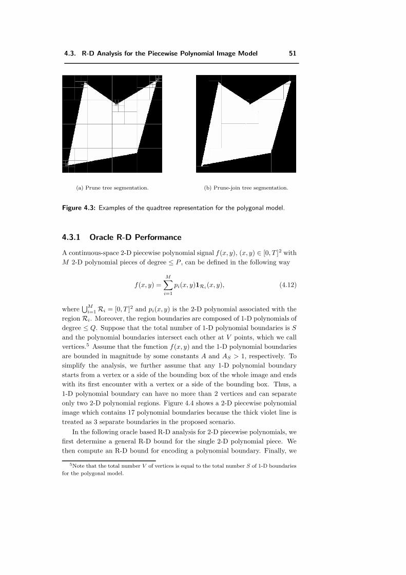
4.3. R-D Analysis for the Piecewise Polynomial Image Model 51
(a) Prune tree segmentation. (b) Prune-join tree segmentation.
Figure 4.3: Examples of the quadtree representation for the polygonal model.
4.3.1 Oracle R-D Performance
A continuous-space 2-D piecewise polynomial signal f(x, y), (x, y) ∈ [0, T ]2 with
M 2-D polynomial pieces of degree ≤ P , can be defined in the following way
f(x, y) =
M∑i=1
pi(x, y)1Ri(x, y), (4.12)
where⋃M
i=1 Ri = [0, T ]2 and pi(x, y) is the 2-D polynomial associated with the
region Ri. Moreover, the region boundaries are composed of 1-D polynomials of
degree ≤ Q. Suppose that the total number of 1-D polynomial boundaries is S
and the polynomial boundaries intersect each other at V points, which we call
vertices.5 Assume that the function f(x, y) and the 1-D polynomial boundaries
are bounded in magnitude by some constants A and AS > 1, respectively. To
simplify the analysis, we further assume that any 1-D polynomial boundary
starts from a vertex or a side of the bounding box of the whole image and ends
with its first encounter with a vertex or a side of the bounding box. Thus, a
1-D polynomial boundary can have no more than 2 vertices and can separate
only two 2-D polynomial regions. Figure 4.4 shows a 2-D piecewise polynomial
image which contains 17 polynomial boundaries because the thick violet line is
treated as 3 separate boundaries in the proposed scenario.
In the following oracle based R-D analysis for 2-D piecewise polynomials, we
first determine a general R-D bound for the single 2-D polynomial piece. We
then compute an R-D bound for encoding a polynomial boundary. Finally, we
5Note that the total number V of vertices is equal to the total number S of 1-D boundaries
for the polygonal model.
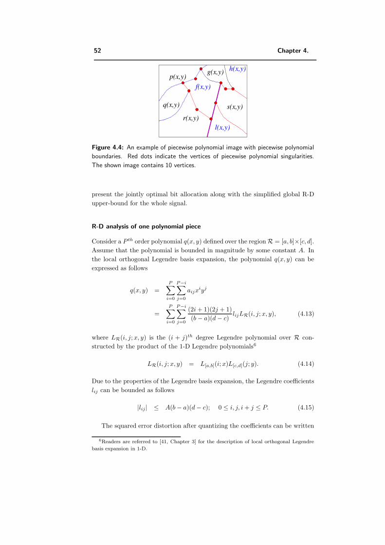
52 Chapter 4.
g(x,y)
s(x,y)
l(x,y)
f(x,y)
h(x,y)p(x,y)
r(x,y)
q(x,y)
Figure 4.4: An example of piecewise polynomial image with piecewise polynomial
boundaries. Red dots indicate the vertices of piecewise polynomial singularities.
The shown image contains 10 vertices.
present the jointly optimal bit allocation along with the simplified global R-D
upper-bound for the whole signal.
R-D analysis of one polynomial piece
Consider a P th order polynomial q(x, y) defined over the region R = [a, b]×[c, d].
Assume that the polynomial is bounded in magnitude by some constant A. In
the local orthogonal Legendre basis expansion, the polynomial q(x, y) can be
expressed as follows
q(x, y) =
P∑i=0
P−i∑j=0
aijxiyj
=P∑
i=0
P−i∑j=0
(2i + 1)(2j + 1)
(b − a)(d − c)lijLR(i, j; x, y), (4.13)
where LR(i, j; x, y) is the (i + j)th degree Legendre polynomial over R con-
structed by the product of the 1-D Legendre polynomials6
LR(i, j; x, y) = L[a,b](i; x)L[c,d](j; y). (4.14)
Due to the properties of the Legendre basis expansion, the Legendre coefficients
lij can be bounded as follows
|lij | ≤ A(b − a)(d − c); 0 ≤ i, j, i + j ≤ P. (4.15)
The squared error distortion after quantizing the coefficients can be written
6Readers are referred to [41, Chapter 3] for the description of local orthogonal Legendre
basis expansion in 1-D.
4.3. R-D Analysis for the Piecewise Polynomial Image Model 53
as follows
Dq =
P∑i=0
P−i∑j=0
((2i + 1)(2j + 1)
(b − a)(d − c)
)2 (lij − lij
)2∫R
L2R(i, j; x, y)
=
P∑i=0
P−i∑j=0
(2i + 1)(2j + 1)
(b − a)(d − c)
(lij − lij
)2
. (4.16)
where lij are the quantized coefficients. Suppose that for each coefficient a
different rij bit uniform quantizer over the range A(b − a)(d − c) with a step
size of 2A(b−a)(d− c)2−rij is used. Thus, the distortion for a polynomial piece
can be bounded as follows
Dq ≤ A2(b − a)(d − c)
P∑i=0
P−i∑j=0
(2i + 1)(2j + 1)2−2rij
Dq ≤ DBq = A0
P∑i=0
P−i∑j=0
(2i + 1)(2j + 1)2−2rij ; A0 = A2(b − a)(d − c).
For a global bit budget of Rq bits, with Rq sufficiently large, the optimal bit
allocation for minimizing the distortion bound DBq can be found by solving the
reverse water-filling problem∂DB
q
∂rij= constant
∑rij = Rq
(4.17)
which results into
rij =2Rq
(P + 1)(P + 2)+
1
2log2
((2i + 1)(2j + 1)
C
), (4.18)
with
C =
∏0≤i,j,i+j≤P
(2i + 1)(2j + 1)
2
(P+1)(P +2)
(4.19)
C ≤ (P + 1)(P + 2)
2; as geometric mean ≤ arithmetic mean. (4.20)
Therefore, the distortion for a single polynomial piece can be bounded as follows
Dq (Rq) ≤ A0
[(P + 1)(P + 2)
2
]2
2−4
(P+1)(P +2)Rq . (4.21)
R-D analysis of one polynomial boundary, which separates 2-D polynomial
pieces
Now, we will analyze the rate-distortion function for encoding one polynomial
boundary s(x) of degree Q, whose coefficients are precisely provided by an oracle.
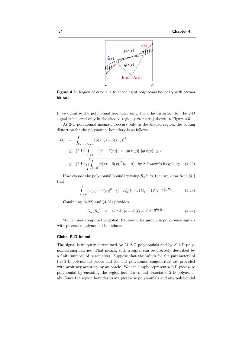
54 Chapter 4.
s(x)^
ba
s(x)
Error−Area
p(x,y)
q(x,y)
Figure 4.5: Region of error due to encoding of polynomial boundary with certain
bit rate.
If we quantize the polynomial boundary only, then the distortion for the 2-D
signal is incurred only in the shaded region (error-area) shown in Figure 4.5.
As 2-D polynomial mismatch occurs only in the shaded region, the coding
distortion for the polynomial boundary is as follows
Ds =
∫Error-Area
(p(x, y) − q(x, y))2
≤ (2A)2∫
[a,b]
|s(x) − s(x)| ; as |p(x, y)|, |q(x, y)| ≤ A.
≤ (2A)2
√∫[a,b]
|s(x) − s(x)|2 (b − a); by Schwartz’s inequality. (4.22)
If we encode the polynomial boundary using Rs bits, then we know from [41]
that ∫[a,b]
|s(x) − s(x)|2 ≤ A2S(b − a) (Q + 1)
22−
2Q+1 Rs . (4.23)
Combining (4.22) and (4.23) provides
Ds (Rs) ≤ 4A2AS(b − a)(Q + 1)2−1
Q+1 Rs . (4.24)
We can now compute the global R-D bound for piecewise polynomial signals
with piecewise polynomial boundaries.
Global R-D bound
The signal is uniquely determined by M 2-D polynomials and by S 1-D poly-
nomial singularities. That means, such a signal can be precisely described by
a finite number of parameters. Suppose that the values for the parameters of
the 2-D polynomial pieces and the 1-D polynomial singularities are provided
with arbitrary accuracy by an oracle. We can simply represent a 2-D piecewise
polynomial by encoding the region-boundaries and associated 2-D polynomi-
als. Since the region boundaries are piecewise polynomials and any polynomial
4.3. R-D Analysis for the Piecewise Polynomial Image Model 55
boundary will be part of two region boundaries, an efficient way to encode a
region boundary is just to specify which 1-D polynomial boundaries are forming
the region boundary in an ordered manner such as clockwise. That means, we
encode all the 1-D polynomial singularities using the standard scalar quantiza-
tion procedure and assign unique indices to 1-D polynomial singularities.7 Now,
the region boundary will be encoded by these indices of the 1-D polynomial sin-
gularities, which form the region boundary. Let us further assume that the
region of support Ri for the polynomial piece pi(x, y) of degree Pi is enclosed
in the rectangular region [ai, bi] × [ci, di]. Thus, if we allocate Rpibits to the
2-D polynomial, then (4.21) provides the following distortion bound due to the
quantization of 2-D polynomial coefficients
Dpi(Rpi
) ≤ A2 (bi − ai) (di − ci)
[(Pi + 1)(Pi + 2)
2
]2
2− 4
(Pi+1)(Pi+2)Rpi .
Similarly, suppose that jth polynomial boundary sj(x) is defined over the
interval [aj , bj ] and has the degree Qj. So if we allocate Rsjbits to the 1-D
polynomial boundary, then (4.24) results into the following distortion bound
due to the quantization of 1-D polynomial boundary coefficients
Dsj
(Rsj
) ≤ 4A2AS(bj − aj)(Qj + 1)2− 1
Qj+1 Rsj .
The global distortion bound for the whole signal will be the sum of the quan-
tization distortion of M 2-D polynomial pieces and the quantization distortion
of S polynomial boundaries. Thus, the global distortion bound can be written
as follows
D ≤M∑i=1
Dpi(Rpi
) +
S∑j=1
Dsj
(Rsj
). (4.25)
However, this R-D function is very complicated and depends on all the polyno-
mial parameters across the whole function. So we make some assumptions to
derive the simplified R-D bound and associated bit allocation strategy:
• All 2-D polynomial pieces and 1-D polynomial boundaries are assumed of
maximum degree P and Q, respectively. This simply means that for a
polynomial of lower degree bits are also allocated to zero coefficients.
• The region of support for each 2-D polynomial piece and 1-D polynomial
boundary is approximated by [0, T ]2 and [0, T ] respectively.
• The bounding box [0, T ]2 of the whole function is known. Thus, we need
not code the bounding box boundary.
7Since the image has S polynomial boundaries and 4 boundaries of the bounding box of
the image, we need log2(S+4) bits to code an index associated with a polynomial boundary.
Moreover, vertex information can be simply obtained by solving the intersection equations of
polynomial boundaries. So each vertex information requires log2 Q bits as side information.
56 Chapter 4.
These assumptions ensure that the reverse water filling R-D optimization
will allocate the same number of bits Rp to each 2-D polynomial and Rs bits to
each polynomial boundary. Therefore, the simplified R-D bound becomes
D(R) ≤ MA2T
2
»(P + 1)(P + 2)
2
–2
2− 4
(P+1)(P +2)Rp + S4A
2AST (Q + 1)2
− 1Q+1
Rs
(4.26)
where the total bit rate is R = MRp + SRs.8 Now, by the usual reverse water
filling technique, we obtain the following optimal bit allocation
Rp =(P + 1)(P + 2)
M(P + 1)(P + 2) + 4S(Q + 1)R + S · C (4.27)
Rs =4(Q + 1)
M(P + 1)(P + 2) + 4S(Q + 1)R − M · C, (4.28)
where C = (P+1)(P+2)(Q+1)M(P+1)(P+2)+4S(Q+1) log2
(M(P+1)(P+2)
4SAS
).
Combining (4.26), (4.27) and (4.28), the simplified global R-D bound be-
comes
D(R) ≤ 2MA2T 2(P + 1)2(P + 2)2SAS2−4
M(P+1)(P +2)+4S(Q+1)R. (4.29)
This concludes that the oracle based method attains an exponentially decay-
ing R-D behavior for 2-D piecewise polynomial functions with piecewise poly-
nomial boundaries. This result can be more formally stated as the following
theorem:
Theorem 4.3 An oracle based method, which simply scalar quantizes the region
boundaries and associated 2-D polynomials, achieves the following exponentially
decaying R-D behavior
D(R) ≤ c102−c11R, (4.30)
where c10 = 2MA2T 2(P +1)2(P +2)2SAS and c11 = 4M(P+1)(P+2)+4S(Q+1) , for
2-D piecewise polynomial images as defined in (4.12).
4.3.2 R-D Analysis of the Prune Quadtree Algorithm
In this section, we present the R-D performance of the prune quadtree algorithm
for 2-D piecewise polynomial signals as defined in (4.12). The presented R-D
analysis closely follows the logic outlined for the polygonal image model. We
first show that the prune quadtree scheme encodes a number of leaves, which
grows linearly with respect to the tree depth J . We then present Theorem 4.4,
which states the suboptimal R-D behavior of the prune quadtree scheme.
Lemma 4.3 The prune quadtree coding algorithm will result in a quadtree with
a number of leaves upper-bounded by (3J + 1)V , where J and V represent the
decomposition depth of the tree and the number of vertices (intersection points
of boundaries) in the 2-D piecewise polynomial signal, respectively.
8In this simplified calculation, we have ignored the side information cost, like the coding
cost of indices of polynomial boundaries, as this cost is negligible at high rates.
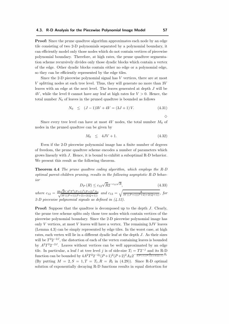
4.3. R-D Analysis for the Piecewise Polynomial Image Model 57
Proof: Since the prune quadtree algorithm approximates each node by an edge
tile consisting of two 2-D polynomials separated by a polynomial boundary, it
can efficiently model only those nodes which do not contain vertices of piecewise
polynomial boundary. Therefore, at high rates, the prune quadtree segmenta-
tion scheme recursively divides only those dyadic blocks which contain a vertex
of the edge. Other dyadic blocks contain either no edge or a polynomial edge,
so they can be efficiently represented by the edge tiles.
Since the 2-D piecewise polynomial signal has V vertices, there are at most
V splitting nodes at each tree level. Thus, they will generate no more than 3V
leaves with an edge at the next level. The leaves generated at depth J will be
4V , while the level 0 cannot have any leaf at high rates for V > 0. Hence, the
total number N0 of leaves in the pruned quadtree is bounded as follows
N0 ≤ (J − 1)3V + 4V = (3J + 1)V. (4.31)
Since every tree level can have at most 4V nodes, the total number M0 of
nodes in the pruned quadtree can be given by
M0 ≤ 4JV + 1. (4.32)
Even if the 2-D piecewise polynomial image has a finite number of degrees
of freedom, the prune quadtree scheme encodes a number of parameters which
grows linearly with J . Hence, it is bound to exhibit a suboptimal R-D behavior.
We present this result as the following theorem.
Theorem 4.4 The prune quadtree coding algorithm, which employs the R-D
optimal parent-children pruning, results in the following asymptotic R-D behav-
ior
DP (R) ≤ c12
√R2−c13
√R, (4.33)
where c12 = 48√
2V A2T 2(P+1)2(P+2)2AS√3V ((P+1)(P+2)+2(Q+1))
and c13 =√
83V ((P+1)(P+2)+2(Q+1)) , for
2-D piecewise polynomial signals as defined in (4.12).
Proof: Suppose that the quadtree is decomposed up to the depth J . Clearly,
the prune tree scheme splits only those tree nodes which contain vertices of the
piecewise polynomial boundary. Since the 2-D piecewise polynomial image has
only V vertices, at most V leaves will have a vertex. The remaining 3JV leaves
(Lemma 4.3) can be simply represented by edge tiles. In the worst case, at high
rates, each vertex will lie in a different dyadic leaf at the depth J . As their sizes
will be T 22−2J , the distortion of each of the vertex containing leaves is bounded
by A2T 22−2J . Leaves without vertices can be well approximated by an edge
tile. In particular, a leaf l at tree level j is of side-size Tl = T 2−j and its R-D
function can be bounded by 4A2T 22−2j(P +1)2(P +2)2AS2−4
2(P+1)(P+2)+4(Q+1)Rl
(By putting M = 2, S = 1, T = Tl, R = Rl in (4.29)). Since R-D optimal
solution of exponentially decaying R-D functions results in equal distortion for
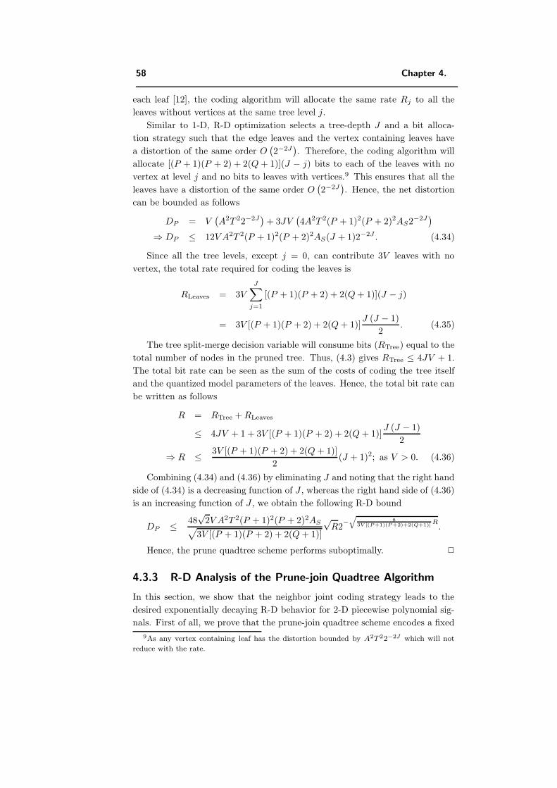
58 Chapter 4.
each leaf [12], the coding algorithm will allocate the same rate Rj to all the
leaves without vertices at the same tree level j.
Similar to 1-D, R-D optimization selects a tree-depth J and a bit alloca-
tion strategy such that the edge leaves and the vertex containing leaves have
a distortion of the same order O(2−2J
). Therefore, the coding algorithm will
allocate [(P + 1)(P + 2) + 2(Q + 1)](J − j) bits to each of the leaves with no
vertex at level j and no bits to leaves with vertices.9 This ensures that all the
leaves have a distortion of the same order O(2−2J
). Hence, the net distortion
can be bounded as follows
DP = V(A2T 22−2J
)+ 3JV
(4A2T 2(P + 1)2(P + 2)2AS2−2J
)⇒ DP ≤ 12V A2T 2(P + 1)2(P + 2)2AS(J + 1)2−2J . (4.34)
Since all the tree levels, except j = 0, can contribute 3V leaves with no
vertex, the total rate required for coding the leaves is
RLeaves = 3V
J∑j=1
[(P + 1)(P + 2) + 2(Q + 1)](J − j)
= 3V [(P + 1)(P + 2) + 2(Q + 1)]J (J − 1)
2. (4.35)
The tree split-merge decision variable will consume bits (RTree) equal to the
total number of nodes in the pruned tree. Thus, (4.3) gives RTree ≤ 4JV + 1.
The total bit rate can be seen as the sum of the costs of coding the tree itself
and the quantized model parameters of the leaves. Hence, the total bit rate can
be written as follows
R = RTree + RLeaves
≤ 4JV + 1 + 3V [(P + 1)(P + 2) + 2(Q + 1)]J (J − 1)
2
⇒ R ≤ 3V [(P + 1)(P + 2) + 2(Q + 1)]
2(J + 1)2; as V > 0. (4.36)
Combining (4.34) and (4.36) by eliminating J and noting that the right hand
side of (4.34) is a decreasing function of J , whereas the right hand side of (4.36)
is an increasing function of J , we obtain the following R-D bound
DP ≤ 48√
2V A2T 2(P + 1)2(P + 2)2AS√3V [(P + 1)(P + 2) + 2(Q + 1)]
√R2
−q
83V [(P+1)(P +2)+2(Q+1)]
R.
Hence, the prune quadtree scheme performs suboptimally.
4.3.3 R-D Analysis of the Prune-join Quadtree Algorithm
In this section, we show that the neighbor joint coding strategy leads to the
desired exponentially decaying R-D behavior for 2-D piecewise polynomial sig-
nals. First of all, we prove that the prune-join quadtree scheme encodes a fixed
9As any vertex containing leaf has the distortion bounded by A2T 22−2J which will not
reduce with the rate.
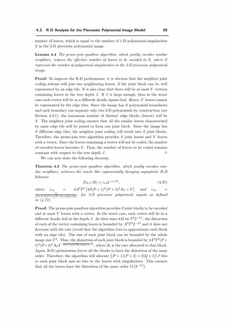
4.3. R-D Analysis for the Piecewise Polynomial Image Model 59
number of leaves, which is equal to the number of 1-D polynomial singularities
S in the 2-D piecewise polynomial image.
Lemma 4.4 The prune-join quadtree algorithm, which jointly encodes similar
neighbors, reduces the effective number of leaves to be encoded to S, where S
represent the number of polynomial singularities in the 2-D piecewise polynomial
image.
Proof: To improve the R-D performance, it is obvious that the neighbor joint
coding scheme will join two neighboring leaves, if the joint block can be well
represented by an edge tile. It is also clear that there will be at most V vertices
containing leaves at the tree depth J . If J is large enough, then in the worst
case each vertex will lie in a different dyadic square leaf. Hence, V leaves cannot
be represented by the edge tiles. Since the image has S polynomial boundaries
and each boundary can separate only two 2-D polynomials by construction (see
Section 4.3.1), the maximum number of distinct edge blocks (leaves) will be
S. The neighbor joint coding ensures that all the similar leaves characterized
by same edge tile will be joined to form one joint block. Since the image has
S different edge tiles, the neighbor joint coding will result into S joint blocks.
Therefore, the prune-join tree algorithm provides S joint leaves and V leaves
with a vertex. Since the leaves containing a vertex will not be coded, the number
of encoded leaves becomes S. Thus, the number of leaves to be coded remains
constant with respect to the tree depth J .
We can now state the following theorem:
Theorem 4.5 The prune-join quadtree algorithm, which jointly encodes sim-
ilar neighbors, achieves the oracle like exponentially decaying asymptotic R-D
behavior
DPJ (R) ≤ c142−c15R, (4.37)
where c14 = 4A2T 2[4S(P + 1)2(P + 2)2AS + V
]and c15 =
2(S+V )[(P+1)(P+2)+2(Q+6)] , for 2-D piecewise polynomial signals as defined
in (4.12).
Proof: The prune-join quadtree algorithm provides S joint blocks to be encoded
and at most V leaves with a vertex. In the worst case, each vertex will lie in a
different dyadic leaf at the depth J . As their sizes will be T 22−2J , the distortion
of each of the vertex containing leaves is bounded by A2T 22−2J and it does not
decrease with the rate (recall that the algorithm tries to approximate each block
with an edge tile). The size of each joint block can be bounded by the whole
image size T 2. Thus, the distortion of each joint block is bounded by 4A2T 2(P +
1)2(P +2)2AS2−4
2(P+1)(P+2)+4(Q+1)Rl , where Rl is the rate allocated to that block.
Again, R-D optimization forces all the blocks to have the distortion of the same
order. Therefore, the algorithm will allocate [(P + 1)(P + 2) + 2(Q + 1)] J bits
to each joint block and no bits to the leaves with singularities. This ensures
that all the leaves have the distortion of the same order O(2−2J
).
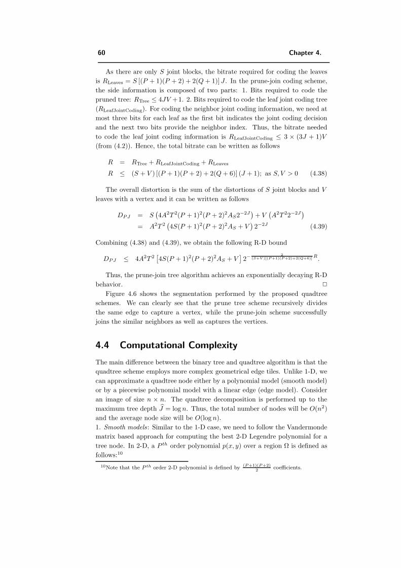
60 Chapter 4.
As there are only S joint blocks, the bitrate required for coding the leaves
is RLeaves = S [(P + 1)(P + 2) + 2(Q + 1)] J . In the prune-join coding scheme,
the side information is composed of two parts: 1. Bits required to code the
pruned tree: RTree ≤ 4JV +1. 2. Bits required to code the leaf joint coding tree
(RLeafJointCoding). For coding the neighbor joint coding information, we need at
most three bits for each leaf as the first bit indicates the joint coding decision
and the next two bits provide the neighbor index. Thus, the bitrate needed
to code the leaf joint coding information is RLeafJointCoding ≤ 3 × (3J + 1)V
(from (4.2)). Hence, the total bitrate can be written as follows
R = RTree + RLeafJointCoding + RLeaves
R ≤ (S + V ) [(P + 1)(P + 2) + 2(Q + 6)] (J + 1); as S, V > 0 (4.38)
The overall distortion is the sum of the distortions of S joint blocks and V
leaves with a vertex and it can be written as follows
DPJ = S(4A2T 2(P + 1)2(P + 2)2AS2−2J
)+ V
(A2T 22−2J
)= A2T 2
(4S(P + 1)2(P + 2)2AS + V
)2−2J (4.39)
Combining (4.38) and (4.39), we obtain the following R-D bound
DPJ ≤ 4A2T 2[4S(P + 1)2(P + 2)2AS + V
]2−
2(S+V )[(P+1)(P+2)+2(Q+6)]
R.
Thus, the prune-join tree algorithm achieves an exponentially decaying R-D
behavior.
Figure 4.6 shows the segmentation performed by the proposed quadtree
schemes. We can clearly see that the prune tree scheme recursively divides
the same edge to capture a vertex, while the prune-join scheme successfully
joins the similar neighbors as well as captures the vertices.
4.4 Computational Complexity
The main difference between the binary tree and quadtree algorithm is that the
quadtree scheme employs more complex geometrical edge tiles. Unlike 1-D, we
can approximate a quadtree node either by a polynomial model (smooth model)
or by a piecewise polynomial model with a linear edge (edge model). Consider
an image of size n × n. The quadtree decomposition is performed up to the
maximum tree depth J = log n. Thus, the total number of nodes will be O(n2)
and the average node size will be O(log n).
1. Smooth models : Similar to the 1-D case, we need to follow the Vandermonde
matrix based approach for computing the best 2-D Legendre polynomial for a
tree node. In 2-D, a P th order polynomial p(x, y) over a region Ω is defined as
follows:10
10Note that the P th order 2-D polynomial is defined by (P+1)(P+2)2
coefficients.
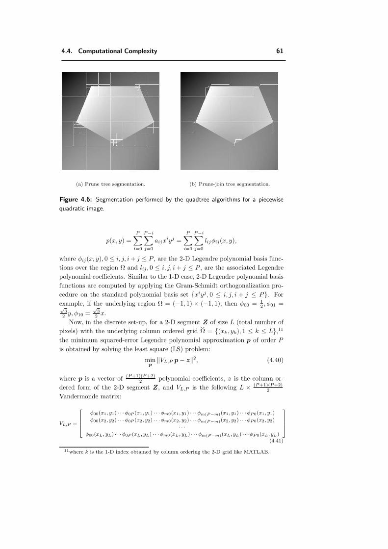
4.4. Computational Complexity 61
(a) Prune tree segmentation. (b) Prune-join tree segmentation.
Figure 4.6: Segmentation performed by the quadtree algorithms for a piecewise
quadratic image.
p(x, y) =
P∑i=0
P−i∑j=0
aijxiyj =
P∑i=0
P−i∑j=0
lijφij(x, y),
where φij(x, y), 0 ≤ i, j, i + j ≤ P , are the 2-D Legendre polynomial basis func-
tions over the region Ω and lij , 0 ≤ i, j, i + j ≤ P , are the associated Legendre
polynomial coefficients. Similar to the 1-D case, 2-D Legendre polynomial basis
functions are computed by applying the Gram-Schmidt orthogonalization pro-
cedure on the standard polynomial basis set xiyj , 0 ≤ i, j, i + j ≤ P. For
example, if the underlying region Ω = (−1, 1) × (−1, 1), then φ00 = 12 , φ01 =√
32 y, φ10 =
√3
2 x.
Now, in the discrete set-up, for a 2-D segment Z of size L (total number of
pixels) with the underlying column ordered grid Ω = (xk, yk), 1 ≤ k ≤ L,11the minimum squared-error Legendre polynomial approximation p of order P
is obtained by solving the least square (LS) problem:
minp
‖VL,P p − z‖2, (4.40)
where p is a vector of (P+1)(P+2)2 polynomial coefficients, z is the column or-
dered form of the 2-D segment Z, and VL,P is the following L × (P+1)(P+2)2
Vandermonde matrix:
VL,P =
26664
φ00(x1, y1) · · ·φ0P (x1, y1) · · ·φm0(x1, y1) · · ·φm(P−m)(x1, y1) · · ·φP0(x1, y1)
φ00(x2, y2) · · ·φ0P (x2, y2) · · ·φm0(x2, y2) · · ·φm(P−m)(x2, y2) · · ·φP0(x2, y2)
· · ·
φ00(xL, yL) · · ·φ0P (xL, yL) · · ·φm0(xL, yL) · · ·φm(P−m)(xL, yL) · · ·φP0(xL, yL)
37775
(4.41)
11where k is the 1-D index obtained by column ordering the 2-D grid like MATLAB.
62 Chapter 4.
Similar to 1-D, the solution to the LS problem in (4.40) is attained effi-
ciently by means of a QR factorization of VL,P with computational cost of
O(L (P+1)(P+2)
2
). The Vandermonde matrix VL,P basically depends on the un-
derlying grid, which is same for all the nodes at the same tree level as all nodes
of a tree level are of the same size. Thus, only one Vandermonde matrix is re-
quired per tree level to compute smooth models. Therefore, we can pre-compute
and store these matrices and their QR factorization for different tree levels and
use them for computing 2-D polynomials for tree nodes just like a look-up ta-
ble. Since the average node-size is O(log n), the overall cost for computing the
smooth models for all the tree nodes will be O(n2 log n). Note that for the
complexity analysis, we include (P+1)(P+2)2 in the complexity constant.
2. Edge models: These are represented by two 2-D polynomials separated by a
linear boundary. Therefore, for each node, we need to search for the best edge
model for a given set of edge orientations like the wedgelet/beamlet dictionary
[17].12 Thus, for each edge-orientation, we need two Vandermonde matrices
associated with the two regions separated by the edge. We can pre-compute
these Vandermonde matrices as given by (4.41). Now, we can compute the
best polynomial surfaces associated with each choice of edge orientation using
the Vandermonde matrix approach. We then select that edge orientation which
leads to the minimum squared error. The edge orientation dictionary and associ-
ated Vandermonde matrices are pre-computed and stored so that the algorithm
can use them like a look-up table.13 Since the average node size is O(log n), the
computational cost for calculating the edge model for a tree node is O(log n).
Hence, the cost for computing the edge models for all the tree nodes will be
O(n2 log n).
For an image of size n×n, the total number of pixels is N = n2. Suppose that
RQ quantizers are utilized for the R-D function computation. Now, by following
the steps of the computational analysis done in Section 2.6 for the 1-D case, it
can be shown that the overall computational costs for both the prune and the
prune-join quadtree algorithms will be O (NRQ log N). Table 4.1 summarizes
the properties of the tree algorithms and compares them with a wavelet coder
and a dynamic programming (DP) coder. But note that DP is not applicable
(NA) in the 2-D case.
12To achieve the theoretical R-D performance for the piecewise polynomial image model,
the algorithm uses the edge-dictionary with O(m2 log m) linear-edge orientations for a node
of size m × m, where m2 is, on average, O(log n). This is also consistent with the high rate
analysis. However, for real images, we limit the maximum number of linear edge choices in
the edge-dictionary to 256, irrespective of the image-size. This is similar as saying that the
linear edge is quantized using no more than 8 bits.13Note that the storage memory requirement is proportional to the size of the edge-
orientation dictionary.
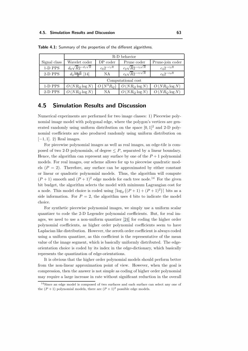
4.5. Simulation Results and Discussion 63
Table 4.1: Summary of the properties of the different algorithms.
R-D behavior
Signal class Wavelet coder DP coder Prune coder Prune-join coder
1-D PPS d0
√R2−d1
√R c02
−c1R c2
√R2−c3
√R c42
−c5R
2-D PPS d2log R
R [14] NA c6
√R2−c7
√R c82
−c9R
Computational cost
1-D PPS O (NRQ log N) O(N3RQ
)O (NRQ log N) O (NRQ log N)
2-D PPS O (NRQ log N) NA O (NRQ log N) O (NRQ log N)
4.5 Simulation Results and Discussion
Numerical experiments are performed for two image classes: 1) Piecewise poly-
nomial image model with polygonal edge, where the polygon’s vertices are gen-
erated randomly using uniform distribution on the space [0, 1]2 and 2-D poly-
nomial coefficients are also produced randomly using uniform distribution on
[−1, 1]. 2) Real images.
For piecewise polynomial images as well as real images, an edge-tile is com-
posed of two 2-D polynomials, of degree ≤ P , separated by a linear boundary.
Hence, the algorithm can represent any surface by one of the P + 1 polynomial
models. For real images, our scheme allows for up to piecewise quadratic mod-
els (P = 2). Therefore, any surface can be approximated by either constant
or linear or quadratic polynomial models. Thus, the algorithm will compute
(P + 1) smooth and (P + 1)2 edge models for each tree node.14 For the given
bit budget, the algorithm selects the model with minimum Lagrangian cost for
a node. This model choice is coded using log2
((P + 1) + (P + 1)2
) bits as a
side information. For P = 2, the algorithm uses 4 bits to indicate the model
choice.
For synthetic piecewise polynomial images, we simply use a uniform scalar
quantizer to code the 2-D Legendre polynomial coefficients. But, for real im-
ages, we need to use a non-uniform quantizer [24] for coding the higher order
polynomial coefficients, as higher order polynomial coefficients seem to have
Laplacian like distribution. However, the zeroth order coefficient is always coded
using a uniform quantizer, as this coefficient is the representative of the mean
value of the image segment, which is basically uniformly distributed. The edge-
orientation choice is coded by its index in the edge-dictionary, which basically
represents the quantization of edge-orientations.
It is obvious that the higher order polynomial models should perform better
from the non-linear approximation point of view. However, when the goal is
compression, then the answer is not simple as coding of higher order polynomial
may require a large increase in rate without significant reduction in the overall
14Since an edge model is composed of two surfaces and each surface can select any one of
the (P + 1) polynomial models, there are (P + 1)2 possible edge models.
64 Chapter 4.
distortion. That is why our scheme selects the appropriate polynomial/edge
tile according to the Lagrangian cost based R-D criterion to achieve better R-D
performance. Simulation results shown in Figure 4.7 indicate that the algorithm
opts for low order polynomial models at low rates. Figure 4.7 also shows the
complex geometrical tiling obtained by the prune-join tree scheme to capture
the geometry of the cameraman image.
For the cameraman image, simulation results show that our scheme prefers
piecewise linear models over piecewise quadratic models at rates less than 0.2
bpp. Even at higher rates, we gain only slightly by using piecewise quadratic
models. Thus, the piecewise linear polynomial model seems to be a good model-
ing choice for cameraman at low rates. Finally, in simulations, we have used only
linear boundary model, which is a good model for edges at low rates, but using
higher order polynomial boundary model may improve the R-D performance at
high rates.
The experimental results shown in Figure 4.8, for the polygonal model, con-
firm the derived theoretical R-D behaviors. In Figures 4.9, 4.11 and 4.12, we
compare the prune-join coding scheme with JPEG2000. Residual images shown
in Figure 4.10 also demonstrate that the prune-join scheme captures the image
geometry more efficiently in comparison to JPEG2000. Figure 4.10(a) also shows
that the residual image obtained by the tree coding scheme essentially contains
only the texture part of the cameraman image. Figure 4.13 compares the prune-
join scheme with JPEG2000 for different regions of the lena image. When the
image is close to the geometrical model (see Figures 4.13 (a), (b)), the prune-join
scheme gives less artifacts. In the textured region (see Figures 4.13 (c), (d)),
the geometrical model fails, and JPEG2000 performs better.
Overall, these simulation results indicate that the prune-join coding scheme
attains not only better visual quality but also higher coding gain in comparison
to JPEG2000. Moreover, Table 4.2 shows that the prune-join tree algorithm
consistently outperforms both the prune tree algorithm and JPEG2000 for dif-
ferent real images at low bit rates. It does so particularly well for the cameraman
image compared to the other images. One possible reason is that the cameraman
image is much closer to the piecewise polynomial image model in comparison to
the other images.
4.6 Conclusions
In this chapter, we have extended our binary tree based coding algorithm to the
2-D case in the form of quadtree based coding algorithm with low computational
complexity of O (N log N). We have also proved that the quadtree based coding
algorithm achieves an exponentially decaying asymptotic R-D behavior for the
piecewise polynomial image model. Numerical simulations (Figure 4.8) also
confirm that the algorithm achieves optimal performance if the input image
belongs to the image model. In addition, simulations show that our quadtree
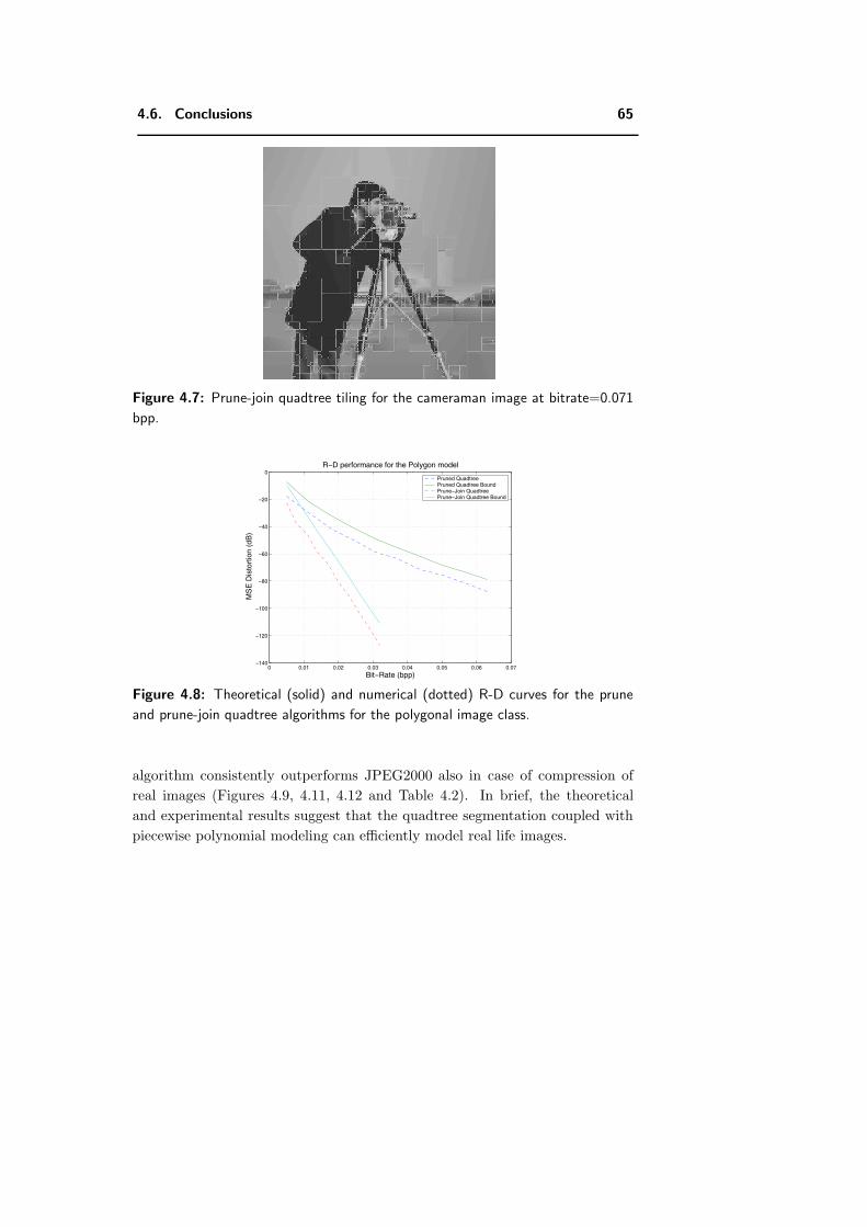
4.6. Conclusions 65
Figure 4.7: Prune-join quadtree tiling for the cameraman image at bitrate=0.071
bpp.
0 0.01 0.02 0.03 0.04 0.05 0.06 0.07−140
−120
−100
−80
−60
−40
−20
0
Bit−Rate (bpp)
MS
E D
isto
rtio
n (d
B)
R−D performance for the Polygon model
Pruned Quadtree Pruned Quadtree BoundPrune−Join QuadtreePrune−Join Quadtree Bound
Figure 4.8: Theoretical (solid) and numerical (dotted) R-D curves for the prune
and prune-join quadtree algorithms for the polygonal image class.
algorithm consistently outperforms JPEG2000 also in case of compression of
real images (Figures 4.9, 4.11, 4.12 and Table 4.2). In brief, the theoretical
and experimental results suggest that the quadtree segmentation coupled with
piecewise polynomial modeling can efficiently model real life images.
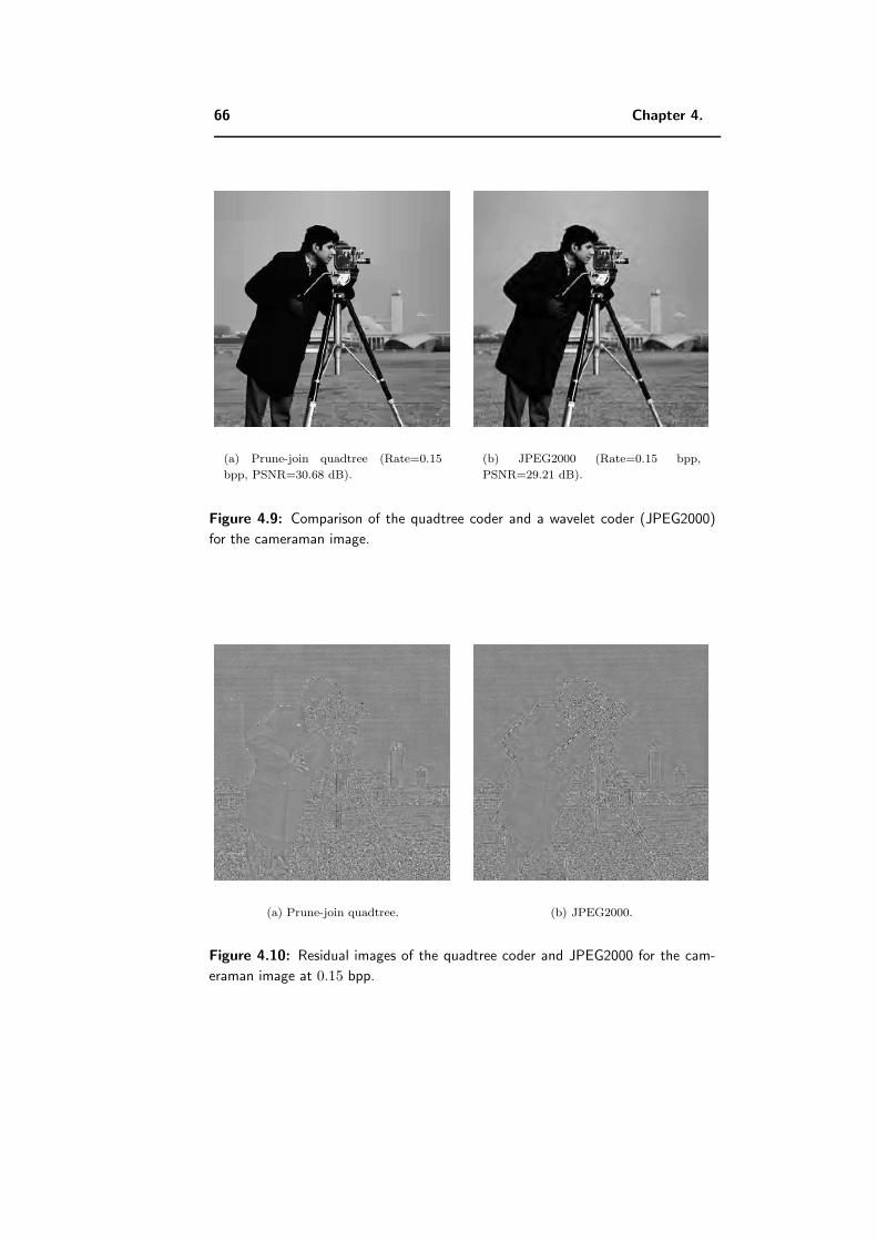
66 Chapter 4.
(a) Prune-join quadtree (Rate=0.15
bpp, PSNR=30.68 dB).
(b) JPEG2000 (Rate=0.15 bpp,
PSNR=29.21 dB).
Figure 4.9: Comparison of the quadtree coder and a wavelet coder (JPEG2000)
for the cameraman image.
(a) Prune-join quadtree. (b) JPEG2000.
Figure 4.10: Residual images of the quadtree coder and JPEG2000 for the cam-
eraman image at 0.15 bpp.
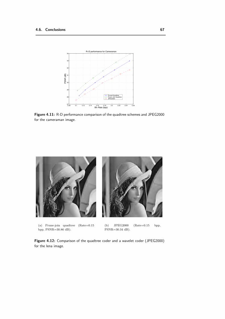
4.6. Conclusions 67
0.08 0.1 0.12 0.14 0.16 0.18 0.2 0.22 0.24 0.2627
28
29
30
31
32
33
34
Bit−Rate (bpp)
PS
NR
(dB
)
R−D performance for Cameraman
Pruned QuadtreePrune−Join QuadtreeJPEG2000
Figure 4.11: R-D performance comparison of the quadtree schemes and JPEG2000
for the cameraman image.
(a) Prune-join quadtree (Rate=0.15
bpp, PSNR=30.86 dB).
(b) JPEG2000 (Rate=0.15 bpp,
PSNR=30.34 dB).
Figure 4.12: Comparison of the quadtree coder and a wavelet coder (JPEG2000)
for the lena image.
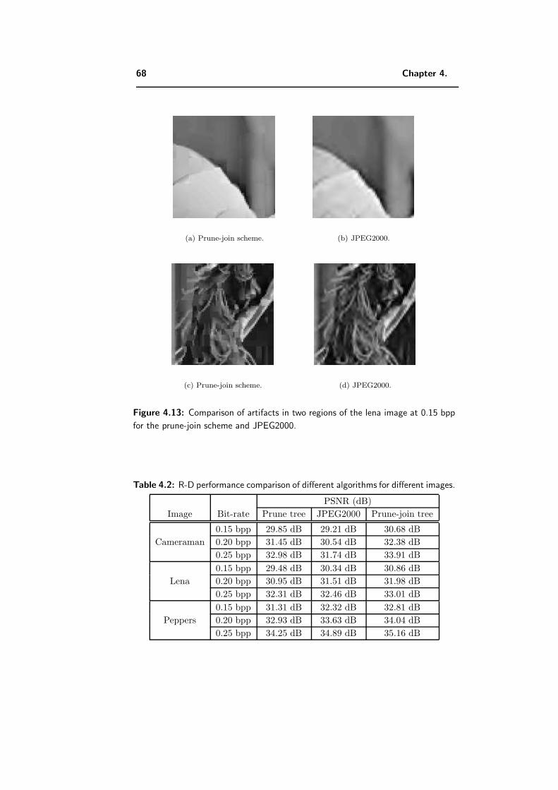
68 Chapter 4.
(a) Prune-join scheme. (b) JPEG2000.
(c) Prune-join scheme. (d) JPEG2000.
Figure 4.13: Comparison of artifacts in two regions of the lena image at 0.15 bpp
for the prune-join scheme and JPEG2000.
Table 4.2: R-D performance comparison of different algorithms for different images.
PSNR (dB)
Image Bit-rate Prune tree JPEG2000 Prune-join tree
0.15 bpp 29.85 dB 29.21 dB 30.68 dB
Cameraman 0.20 bpp 31.45 dB 30.54 dB 32.38 dB
0.25 bpp 32.98 dB 31.74 dB 33.91 dB
0.15 bpp 29.48 dB 30.34 dB 30.86 dB
Lena 0.20 bpp 30.95 dB 31.51 dB 31.98 dB
0.25 bpp 32.31 dB 32.46 dB 33.01 dB
0.15 bpp 31.31 dB 32.32 dB 32.81 dB
Peppers 0.20 bpp 32.93 dB 33.63 dB 34.04 dB
0.25 bpp 34.25 dB 34.89 dB 35.16 dB
Chapter 5
Piecewise Smooth Images and
Quadtree Segmentation
Algorithms
5.1 Introduction
Recent studies have shown that real-life images can be well approximated as
a sum of 2-D piecewise smooth functions and textures [24]. In this represen-
tation, the piecewise smooth part represents the underlying regular structure
of the image, while texture represents the random noise like features of the
image. Numerical simulations performed in Section 4.5 of the previous chap-
ter clearly show that if the real image is compressed at low rates, then only
the regular structure of the image is captured. This means that a compression
scheme must be able to code the regular structure of the image efficiently to
achieve higher R-D performance. This prompts us to investigate whether the
proposed quadtree based segmentation algorithms can achieve the correct R-D
behavior for 2-D piecewise smooth images. In the next section, we consider
2-D smooth functions and show that the quadtree algorithms achieve the oracle
like R-D performance (Theorem 5.1). We then analyze the R-D performance
for 2-D piecewise smooth functions with smooth boundaries in Section 5.3. In
this section, we also prove a strong negative result in the form of Theorem 5.2
which states that, unlike the 1-D case, a 2-D piecewise smooth function cannot
be decomposed as a sum of a 2-D piecewise polynomial and a smooth residual
function. However, this result poses no obstacle to the proposed tree algo-
rithms in attaining a near-optimal R-D behavior, as shown by Theorem 5.3 and
(5.27), for 2-D piecewise smooth functions with smooth boundaries. Section 5.4
shows experimental results, which also confirm the derived R-D behaviors of the
quadtree algorithms. Finally, concluding remarks are presented in Section 5.5.
69
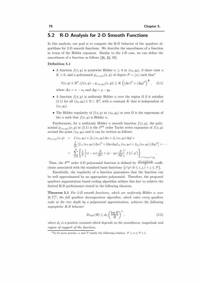
70 Chapter 5.
5.2 R-D Analysis for 2-D Smooth Functions
In this analysis, our goal is to compute the R-D behavior of the quadtree al-
gorithms for 2-D smooth functions. We describe the smoothness of a function
in terms of the Holder exponent. Similar to the 1-D case, we can define the
smoothness of a function as follows [26, 32, 33]:
Definition 5.1
• A function f(x, y) is pointwise Holder α ≥ 0 at (x0, y0), if there exist a
K > 0, and a polynomial p(x0,y0)(x, y) of degree P = α such that1
∀(x, y) ∈ R2, |f(x, y) − p(x0,y0)(x, y)| ≤ K
((∆x)
2+ (∆y)
2)α
2
, (5.1)
where ∆x = x − x0 and ∆y = y − y0.
• A function f(x, y) is uniformly Holder α over the region Ω if it satisfies
(5.1) for all (x0, y0) ∈ Ω ⊂ R2, with a constant K that is independent of
(x0, y0).
• The Holder regularity of f(x, y) at (x0, y0) or over Ω is the supremum of
the α such that f(x, y) is Holder α.
Furthermore, for a uniformly Holder α smooth function f(x, y), the poly-
nomial p(x0,y0)(x, y) in (5.1) is the P th order Taylor series expansion of f(x, y)
around the point (x0, y0) and it can be written as follows:
p(x0,y0)(x, y) = f (x0, y0) + [fx (x0, y0)∆x + fy (x0, y0)∆y] +
1
2!
ˆfxx (x0, y0) (∆x)2 + 2∆x∆yfxy (x0, y0) + fyy (x0, y0) (∆y)2
˜+ · · ·
=
PXi=0
(1
i!
»(x − x0)
∂
∂x′ + (y − y0)∂
∂y′
–i
f`x′, y
′´)x′=x0,y′=y0
.
Thus, the P th order 2-D polynomial function is defined by (P+1)(P+2)2 coeffi-
cients associated with the standard basis functionsxiyj; 0 ≤ i, j, i + j ≤ P
.
Essentially, the regularity of a function guarantees that the function can
be well approximated by an appropriate polynomial. Therefore, the proposed
quadtree segmentation based coding algorithm utilizes this fact to achieve the
desired R-D performance stated in the following theorem.
Theorem 5.1 For 2-D smooth functions, which are uniformly Holder α over
[0, T ]2, the full quadtree decomposition algorithm, which codes every quadtree
node at the tree depth by a polynomial approximation, achieves the following
asymptotic R-D behavior
DFull (R) ≤ d3
(log R
R
)α
, (5.2)
where d3 is a positive constant which depends on the smoothness, magnitude and
region of support of the function.
1To be more precise, α and P satisfy the following relation: P < α ≤ P + 1.
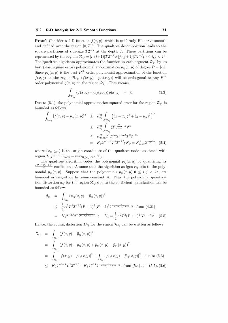
5.2. R-D Analysis for 2-D Smooth Functions 71
Proof: Consider a 2-D function f(x, y), which is uniformly Holder α smooth
and defined over the region [0, T ]2. The quadtree decomposition leads to the
square partitions of side-size T 2−J at the depth J . These partitions can be
represented by the regions Rij = [i, (i+1)]T 2−J × [j, (j+1)]T 2−J ; 0 ≤ i, j < 2J .
The quadtree algorithm approximates the function in each segment Rij by its
best (least square error) polynomial approximation pij(x, y) of degree P = α.Since pij(x, y) is the best P th order polynomial approximation of the function
f(x, y) on the region Rij , (f(x, y) − pij(x, y)) will be orthogonal to any P th
order polynomial q(x, y) on the region Rij . That means,∫Rij
(f(x, y) − pij(x, y)) q(x, y) = 0. (5.3)
Due to (5.1), the polynomial approximation squared error for the region Rij is
bounded as follows∫Rij
[f(x, y) − pij(x, y)]2 ≤ K2
ij
∫Rij
((x − xij)
2+ (y − yij)
2)α
≤ K2ij
∫Rij
(T√
22−J)2α
≤ K2max2
αT 2α2−2αJT 22−2J
= K02−2αJT 22−2J ; K0 = K2
max2αT 2α. (5.4)
where (xij , yij) is the origin coordinate of the quadtree node associated with
region Rij and Kmax = max0≤i,j<2J Kij .
The quadtree algorithm codes the polynomial pij(x, y) by quantizing its(P+1)(P+2)
2 coefficients. Assume that the algorithm assigns rij bits to the poly-
nomial pij(x, y). Suppose that the polynomials pij(x, y), 0 ≤ i, j < 2J , are
bounded in magnitude by some constant A. Thus, the polynomial quantiza-
tion distortion dij for the region Rij due to the coefficient quantization can be
bounded as follows
dij =
∫Rij
(pij(x, y) − pij(x, y))2
≤ 1
4A2T 22−2J(P + 1)2(P + 2)22−
4(P+1)(P+2) rij ; from (4.21)
= K12−2J2−
4(P+1)(P +2)
rij ; K1 =1
4A2T 2(P + 1)2(P + 2)2. (5.5)
Hence, the coding distortion Dij for the region Rij can be written as follows
Dij =
∫Rij
(f(x, y) − pij(x, y))2
=
∫Rij
(f(x, y) − pij(x, y) + pij(x, y) − pij(x, y))2
=
∫Rij
[f(x, y) − pij(x, y)]2
+
∫Rij
[pij(x, y) − pij(x, y)]2, due to (5.3)
≤ K02−2αJT 22−2J + K12
−2J2−4
(P+1)(P +2)rij , from (5.4) and (5.5). (5.6)
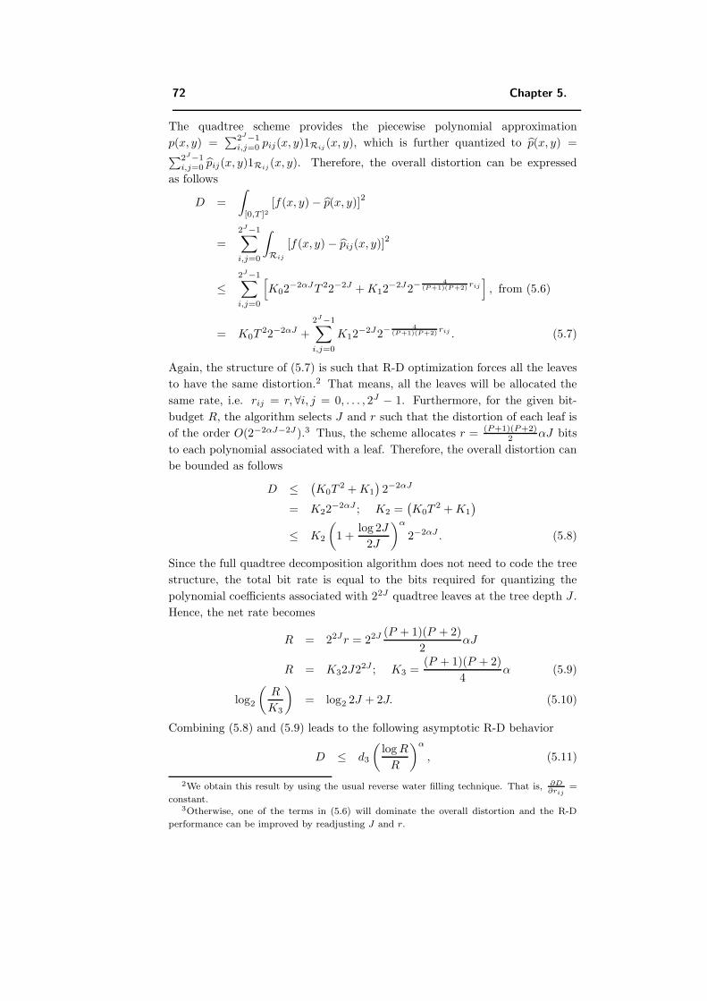
72 Chapter 5.
The quadtree scheme provides the piecewise polynomial approximation
p(x, y) =∑2J−1
i,j=0 pij(x, y)1Rij(x, y), which is further quantized to p(x, y) =∑2J−1
i,j=0 pij(x, y)1Rij(x, y). Therefore, the overall distortion can be expressed
as follows
D =
∫[0,T ]2
[f(x, y) − p(x, y)]2
=
2J−1∑i,j=0
∫Rij
[f(x, y) − pij(x, y)]2
≤2J−1∑i,j=0
[K02
−2αJT 22−2J + K12−2J2−
4(P+1)(P +2) rij
], from (5.6)
= K0T22−2αJ +
2J−1∑i,j=0
K12−2J2−
4(P+1)(P +2)
rij . (5.7)
Again, the structure of (5.7) is such that R-D optimization forces all the leaves
to have the same distortion.2 That means, all the leaves will be allocated the
same rate, i.e. rij = r, ∀i, j = 0, . . . , 2J − 1. Furthermore, for the given bit-
budget R, the algorithm selects J and r such that the distortion of each leaf is
of the order O(2−2αJ−2J ).3 Thus, the scheme allocates r = (P+1)(P+2)2 αJ bits
to each polynomial associated with a leaf. Therefore, the overall distortion can
be bounded as follows
D ≤ (K0T
2 + K1
)2−2αJ
= K22−2αJ ; K2 =
(K0T
2 + K1
)≤ K2
(1 +
log 2J
2J
)α
2−2αJ . (5.8)
Since the full quadtree decomposition algorithm does not need to code the tree
structure, the total bit rate is equal to the bits required for quantizing the
polynomial coefficients associated with 22J quadtree leaves at the tree depth J .
Hence, the net rate becomes
R = 22Jr = 22J (P + 1)(P + 2)
2αJ
R = K32J22J ; K3 =(P + 1)(P + 2)
4α (5.9)
log2
(R
K3
)= log2 2J + 2J. (5.10)
Combining (5.8) and (5.9) leads to the following asymptotic R-D behavior
D ≤ d3
(log R
R
)α
, (5.11)
2We obtain this result by using the usual reverse water filling technique. That is, ∂D∂rij
=
constant.3Otherwise, one of the terms in (5.6) will dominate the overall distortion and the R-D
performance can be improved by readjusting J and r.
5.2. R-D Analysis for 2-D Smooth Functions 73
where d3 = K2
(K2
3 + 1)α
, K2 =[K2
max2αT 2α + A2(P+1)2(P+2)2
4
]T 2 and K3 =
(P+1)(P+2)4 α.
Therefore, the full quadtree decomposition algorithm achieves the stated asymp-
totic R-D behavior.
Corollary 5.1 The prune quadtree coding algorithm achieves the following
asymptotic R-D behavior
DPrune (R) ≤ d3
(log R
R
)α
, (5.12)
for 2-D smooth functions, which are uniformly Holder α over [0, T ]2.
Proof: Since the prune quadtree algorithm results into the full quadtree algo-
rithm, when no pruning is performed, the prune quadtree scheme will perform
at least as well as the full tree scheme. Thus, the prune tree scheme will also
achieve the R-D behavior given by (5.12).
Corollary 5.2 The prune-join quadtree algorithm achieves the following
asymptotic R-D behavior
DPrune-Join (R) ≤ d3
(log R
R
)α
, (5.13)
for 2-D smooth functions, which are uniformly Holder α over [0, T ]2.
Proof: Since the prune-join quadtree algorithm leads to the full quadtree algo-
rithm, when neither pruning nor neighbor joining is performed, the prune-join
tree scheme will perform at least as well as the full tree scheme. Hence, the
prune-join tree scheme will also achieve the asymptotic R-D behavior indicated
by (5.13).
Therefore, we can conclude that the full, the prune and the prune-join
schemes achieve the similar asymptotic R-D behavior(d3
(log R
R
)α)for 2-D
Holder α smooth functions. However, note that the given R-D bound is a weak
upper-bound for both the prune and the prune-join coding schemes.
Remark: It is worth noticing that the presented R-D analysis can be extended
to the higher dimensional N -D case by using 2N -tree segmentation method,
where 2N simply indicates the number of children of a node obtained by its
decomposition. That means, the binary tree is 21-tree, the quadtree is 22-tree,
the oct-tree is 23-tree, and so on. By following the same logic of Theorem 5.1,
one can show that, for N -D uniformly Holder α smooth functions, the full 2N -
tree decomposition algorithm, which codes every tree node at the tree depth
by a N -D polynomial approximation, achieves the following asymptotic R-D
behavior
DFull (R) ≤ d4
(log R
R
) 2αN
, (5.14)
74 Chapter 5.
for some positive constant d4 which depends on the smoothness, magnitude and
region of support of the function.
We can notice that, by putting N = 1 and N = 2 in (5.14), we obtain the R-
D behaviors derived for the binary tree and quadtree algorithms, respectively.
5.3 R-D Analysis for 2-D Piecewise Smooth Func-
tions
Similar to the 1-D case, we can define a 2-D piecewise smooth function f(x, y),
(x, y) ∈ [0, T ]2 with M smooth pieces, in the following way
f(x, y) =
M∑i=1
fi(x, y)1Ri(x, y), (5.15)
where⋃M
i=1 Ri = [0, T ]2 and fi(x, y), the function associated with the region
Ri, is uniformly Holder α over [0, T ]2. Furthermore, region boundaries are
also 1-D piecewise smooth curves whose pieces are uniformly Holder α over
[0, T ]. Since the class of 2-D piecewise smooth signals is much more general
than the class of piecewise polynomial images, it can better model real images
encountered in practice. That is why we will study the R-D behaviors of the
quadtree algorithms for piecewise smooth functions in this section.
For the 1-D case, it has been shown in [21] that a 1-D piecewise smooth
function, whose pieces are Holder α-smooth, can be expressed as a sum of a 1-D
piecewise polynomial with pieces of maximum degree P = α and a residual
function which is Holder α-smooth. However, we show in the following theorem
that such a decomposition cannot be performed in 2-D.
Theorem 5.2 A 2-D piecewise smooth function f(x, y), whose pieces are uni-
formly Holder α-smooth, cannot be written as a sum of a 2-D piecewise polyno-
mial p(x, y) with finite number of pieces of finite degree and a residual function
r(x, y) which is uniformly Holder α-smooth.
Proof: We prove this theorem by contradiction. Let us consider a very sim-
ple piecewise smooth function, which is composed of only two 2-D α-smooth
functions separated by a smooth boundary. Assume that there exists a 2-D
piecewise polynomial with pieces of finite degrees, which make the residual func-
tion α-smooth. This implies that the 2-D piecewise polynomial representation
completely kills the singularity along the smooth boundary. Hence, the polyno-
mials need to eliminate the singularities at infinitely many points on the smooth
boundary. This means that they need to satisfy infinite number of constraints.
However, we know that no polynomial of finite degree can satisfy infinitely many
constraints. Therefore, we cannot find a finite degree 2-D piecewise polynomial
representation, which completely kills the singularity along the smooth bound-
ary. Thus, a 2-D piecewise smooth function f(x, y), whose pieces are Holder
5.3. R-D Analysis for 2-D Piecewise Smooth Functions 75
α-smooth, cannot be expressed as a sum of a 2-D piecewise polynomial p(x, y)
with finite number of pieces of finite degree and a residual function r(x, y) which
is Holder α-smooth.
Moreover, this results holds even if the boundary is a 1-D polynomial func-
tion. This is because still 2-D polynomials have to satisfy infinite number of
constraints to eliminate singularities at infinitely many points on the polynomial
boundary. Again, since no polynomial of finite degree can satisfy infinitely many
constraints, we cannot find a finite degree 2-D piecewise polynomial represen-
tation, which completely kills the singularity along the polynomial boundary.
Remark: An important practical implication of Theorem 5.2 is that a two
stage compression system, piecewise polynomial approximation followed by a
residual coder, cannot improve the overall R-D performance compared to simple
piecewise polynomial approximation. This is because the residual function,
despite having low energy, is not smooth and is geometrically more complex
which makes it difficult to compress efficiently.
5.3.1 R-D Analysis for the Horizon Model
For the sake of simplicity, we carry out the analysis for a simpler image model
known as the Horizon model [16]. An image f(x, y) of the Horizon model is
defined on the unit square [0, 1]2 in the following way:
f(x, y) = 1y≥b(x), 0 ≤ x, y ≤ 1, (5.16)
where the Horizon boundary function b(x) is uniformly Holder α, and b(x) has
finite length inside the unit square.
Oracle R-D behavior
Since the Horizon model image is white above the boundary and black below the
boundary, it has the complexity of a 1-D function. Therefore, when coding such
an image, an oracle based method could simply spend all the available bit rate
to code the smooth edge. Given a bit budget R, coding the edge b produces b
and the corresponding 2-D function f . The distortion can be written as follows
D(R, f) =
∫[0,1]2
(f − f)2 ≤∫
[0,1]
|b − b|
≤√∫
[0,1]
(b − b)2 =√
D(R, b),
where the second inequality comes from the Schwartz’s inequality. Since the
edge b(x) is uniformly Holder α smooth, coding it using a wavelet basis with
enough vanishing moment gives D(R, b) ∼ R−2α [9]. Thus, the oracle R-D
behavior for the Horizon model is as follows
D(R, f) ∼ R−α. (5.17)
76 Chapter 5.
R-D performance of the prune quadtree algorithm
Theorem 5.3 For the Horizon model with uniformly Holder α smooth bound-
ary, the prune quadtree coding algorithm achieves the following asymptotic R-D
behavior
DPrune (R) ∼ d5
(log R
R
)α
, (5.18)
where d5 is a positive constant which depends on the smoothness, magnitude and
length of the boundary function.
Proof: Assume that the Horizon model image has an edge of finite length
LEdge. Suppose that the quadtree decomposition is performed up to the depth
J . Any tree node either contains the edge segment or can be represented by a
smooth region (black or white). The quadtree nodes without edge will be simply
assigned 1 bit to indicate if it is black or white. This ensures that smooth nodes
are represented losslessly (zero distortion) just using 1 bit. However, an edge
block is approximated by an edge tile which consists of two constant regions
separated by a polynomial approximation of the edge segment. That means, at
high rates, edge blocks need to be further divided to capture the edge and to
improve the R-D performance. Therefore, at high rates, our quadtree algorithm
recursively divides the blocks with edges only. Let nj be the number of dyadic
squares at tree level j that intersect with edge curve on the unit square. Since
the edge has finite length LEdge, we have
nj ∼ LEdge2j . (5.19)
Since only edge nodes are divided further, the total number NAll of nodes can
be counted as the number of children of all dyadic edge squares up to level J −1
that intersect with the boundary b(x). That means,
NAll ≤ 4J−1∑j=0
nj
NAll ∼ 4LEdge2J , using (5.19). (5.20)
Clearly, at high rates, all the edge leaves will lie at the tree-depth J in the
worst case scenario. Hence, the number NEdge of edge leaves can be bounded
as follows: NEdge ≤ nJ ∼ LEdge2J . Thus, the number of leaves to be coded
grows exponentially with respect to the depth J . To code an edge leaf i, the tree
scheme approximates its edge segment by a polynomial pi of degree P = αand code the polynomial by quantizing its coefficients.4 If we allocate ri bits to
the edge leaf i of side-size 2−J , the associated distortion Di can be bounded as
4The scheme also uses 1 bit to indicate the value (black or white) of the region above the
polynomial.
5.3. R-D Analysis for 2-D Piecewise Smooth Functions 77
follows
Di =
∫|b(x) − pi(x)|
≤√∫
|b(x) − pi(x)|2 · 2−J , from Schwartz’s inequality
≤√(
K02−2αJ2−J + A202
−J2−2
P+1ri
)2−J , using (3.7)
≤√
K02−αJ2−J + A02
−J2−1
P+1 ri . (5.21)
The total distortion is the sum of the distortions of all tree leaves. Since leaves
without edges are coded losslessly, the net distortion becomes
D =
NEdge∑i=1
Di
≤ NEdge
√K02
−αJ2−J +
NEdge∑i=1
A02−J2−
1P+1 ri . (5.22)
Clearly, R-D optimization will force all the edge leaves to have the equal dis-
tortion. That means, all the edge leaves will be allocated the same rate, i.e.
ri = r, i = 1, . . . , NEdge. Moreover, for the given bit-budget R, the algo-
rithm selects J and r such that the distortion of each edge leaf is of the or-
der O(2−αJ−J ).5 Hence, the coding scheme allocates r = (P + 1)αJ bits to
each polynomial associated with a leaf. Therefore, the overall distortion can be
bounded as follows
D ≤ NEdge
(√K0 + A0
)2−αJ2−J
∼ LEdge
(√K0 + A0
)2−αJ ; as NEdge ∼ LEdge2
J
∼ K12−αJ ; K1 = LEdge
(√K0 + A0
). (5.23)
The total bitrate is the sum of the costs of coding the tree structure and the
quantized model parameters of the smooth and edge leaves. The bitrate RTree
required to code the tree structure is equal to the total number NAll of nodes
in the pruned tree. Thus, (5.20) gives RTree ∼ 4LEdge2J . Since a smooth leaf
is coded using only 1 bit, the bitrate RSmoothLeaves needed for smooth leaves is
bounded by NAll. That is, RSmoothLeaves ∼ 4LEdge2J . To code the edge leaves,
the algorithm uses REdgeLeaves = NEdge((P + 1)αJ + 1) bits.6 Hence, the total
5Otherwise, one of the terms in (5.21) will dominate the overall distortion and the R-D
performance can be improved by reselecting J and r.6Recall that the scheme uses 1 bit to code the value (black or white) of the region above
the polynomial.
78 Chapter 5.
bitrate can be computed as follows
R = RTree + RSmoothLeaves + REdgeLeaves
∼ 4LEdge2J + 4LEdge2
J + LEdge2J((P + 1)αJ + 1)
∼ LEdge(P + 1)(α + 9)J2J ; as at high rates J > 1
∼ K2J2J ; K2 = LEdge(P + 1)(α + 9). (5.24)
Combining (5.23) and (5.24) provides the following asymptotic R-D behavior
D ∼ d5
(log R
R
)α
, (5.25)
where d5 = K1Kα2 = LEdge
(√K0 + A0
)(LEdge(P + 1)(α + 9))
α.
Therefore, the prune quadtree algorithm achieves the announced R-D perfor-
mance.
Corollary 5.3 The prune-join quadtree algorithm achieves the following
asymptotic R-D behavior
DPrune-Join(R) ∼ d5
(log R
R
)α
, (5.26)
for the Horizon model with uniformly Holder α smooth boundary.
Proof: Since the prune-join quadtree algorithm results in the prune quadtree
algorithm, when no neighbor joining is performed, the prune-join tree scheme
will perform at least as well as the prune tree scheme. Hence, the prune-join
tree scheme will also achieve the asymptotic R-D behavior indicated by (5.26).
Therefore, for the Horizon model, both the prune and prune-join tree al-
gorithms achieve the near-optimal asymptotic R-D decay(d5
(log R
R
)α). The
suboptimality factor (log R)α is clearly a penalty for using a tree structure.
Furthermore, by combining the coding strategy for the Horizon model with
that of the 1-D piecewise smooth signals given in Section 3.3.2, it is straightfor-
ward to show that this result will also hold when the edge curve b(x) is piecewise
smooth.7 The key point is that the tree nodes with singular points of the edge
curve cannot be well approximated by edge tiles. So these nodes will be decom-
posed deeper in comparison to the nodes which contain edge segment without
any singular point of the edge curve. Our earlier analysis has shown that R-D
optimization forces all the tree leaves to have the distortion of the same order.
Suppose that the tree nodes with singular points of the edge curve are decom-
posed up to level J , so their distortions are of the order O(2−2J
). Similarly,
if the edge-nodes, which contain an edge segment without any singular point
of the edge curve, are decomposed up to level J1, then their distortions are of
7We have already shown in Section 3.3.2 that the binary tree algorithms achieve the correct
R-D behavior for 1-D piecewise smooth signals.
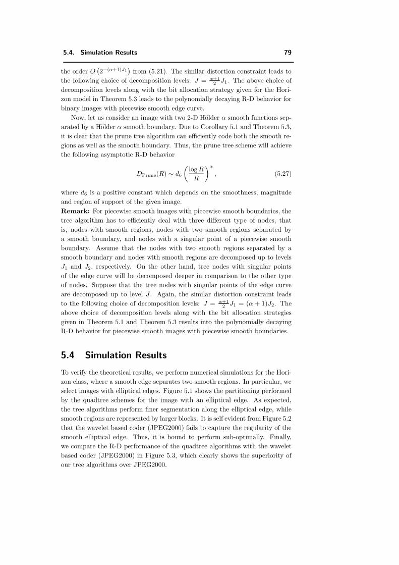
5.4. Simulation Results 79
the order O(2−(α+1)J1
)from (5.21). The similar distortion constraint leads to
the following choice of decomposition levels: J = α+12 J1. The above choice of
decomposition levels along with the bit allocation strategy given for the Hori-
zon model in Theorem 5.3 leads to the polynomially decaying R-D behavior for
binary images with piecewise smooth edge curve.
Now, let us consider an image with two 2-D Holder α smooth functions sep-
arated by a Holder α smooth boundary. Due to Corollary 5.1 and Theorem 5.3,
it is clear that the prune tree algorithm can efficiently code both the smooth re-
gions as well as the smooth boundary. Thus, the prune tree scheme will achieve
the following asymptotic R-D behavior
DPrune(R) ∼ d6
(log R
R
)α
, (5.27)
where d6 is a positive constant which depends on the smoothness, magnitude
and region of support of the given image.
Remark: For piecewise smooth images with piecewise smooth boundaries, the
tree algorithm has to efficiently deal with three different type of nodes, that
is, nodes with smooth regions, nodes with two smooth regions separated by
a smooth boundary, and nodes with a singular point of a piecewise smooth
boundary. Assume that the nodes with two smooth regions separated by a
smooth boundary and nodes with smooth regions are decomposed up to levels
J1 and J2, respectively. On the other hand, tree nodes with singular points
of the edge curve will be decomposed deeper in comparison to the other type
of nodes. Suppose that the tree nodes with singular points of the edge curve
are decomposed up to level J . Again, the similar distortion constraint leads
to the following choice of decomposition levels: J = α+12 J1 = (α + 1)J2. The
above choice of decomposition levels along with the bit allocation strategies
given in Theorem 5.1 and Theorem 5.3 results into the polynomially decaying
R-D behavior for piecewise smooth images with piecewise smooth boundaries.
5.4 Simulation Results
To verify the theoretical results, we perform numerical simulations for the Hori-
zon class, where a smooth edge separates two smooth regions. In particular, we
select images with elliptical edges. Figure 5.1 shows the partitioning performed
by the quadtree schemes for the image with an elliptical edge. As expected,
the tree algorithms perform finer segmentation along the elliptical edge, while
smooth regions are represented by larger blocks. It is self evident from Figure 5.2
that the wavelet based coder (JPEG2000) fails to capture the regularity of the
smooth elliptical edge. Thus, it is bound to perform sub-optimally. Finally,
we compare the R-D performance of the quadtree algorithms with the wavelet
based coder (JPEG2000) in Figure 5.3, which clearly shows the superiority of
our tree algorithms over JPEG2000.
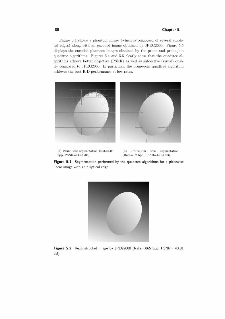
80 Chapter 5.
Figure 5.4 shows a phantom image (which is composed of several ellipti-
cal edges) along with an encoded image obtained by JPEG2000. Figure 5.5
displays the encoded phantom images obtained by the prune and prune-join
quadtree algorithms. Figures 5.4 and 5.5 clearly show that the quadtree al-
gorithms achieve better objective (PSNR) as well as subjective (visual) qual-
ity compared to JPEG2000. In particular, the prune-join quadtree algorithm
achieves the best R-D performance at low rates.
(a) Prune tree segmentation (Rate=.03
bpp, PSNR=44.43 dB).
(b) Prune-join tree segmentation
(Rate=.02 bpp, PSNR=44.24 dB).
Figure 5.1: Segmentation performed by the quadtree algorithms for a piecewise
linear image with an elliptical edge.
Figure 5.2: Reconstructed image by JPEG2000 (Rate=.065 bpp, PSNR= 43.81
dB).
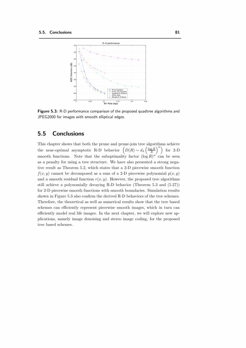
5.5. Conclusions 81
0 0.05 0.1 0.15 0.2 0.25−65
−60
−55
−50
−45
−40
−35
−30
−25
Bit−Rate (bpp)
MS
E D
isto
rtio
n (d
B)
R−D performance
Prune QuadtreePrune−Join QuadtreeQuadtree R−D BoundJPEG−2000Wavelet R−D Bound
Figure 5.3: R-D performance comparison of the proposed quadtree algorithms and
JPEG2000 for images with smooth elliptical edges.
5.5 Conclusions
This chapter shows that both the prune and prune-join tree algorithms achieve
the near-optimal asymptotic R-D behavior(D(R) ∼ d3
(log R
R
)α)for 2-D
smooth functions. Note that the suboptimality factor (log R)α can be seen
as a penalty for using a tree structure. We have also presented a strong nega-
tive result as Theorem 5.2, which states that a 2-D piecewise smooth function
f(x, y) cannot be decomposed as a sum of a 2-D piecewise polynomial p(x, y)
and a smooth residual function r(x, y). However, the proposed tree algorithms
still achieve a polynomially decaying R-D behavior (Theorem 5.3 and (5.27))
for 2-D piecewise smooth functions with smooth boundaries. Simulation results
shown in Figure 5.3 also confirm the derived R-D behaviors of the tree schemes.
Therefore, the theoretical as well as numerical results show that the tree based
schemes can efficiently represent piecewise smooth images, which in turn can
efficiently model real life images. In the next chapter, we will explore new ap-
plications, namely image denoising and stereo image coding, for the proposed
tree based schemes.
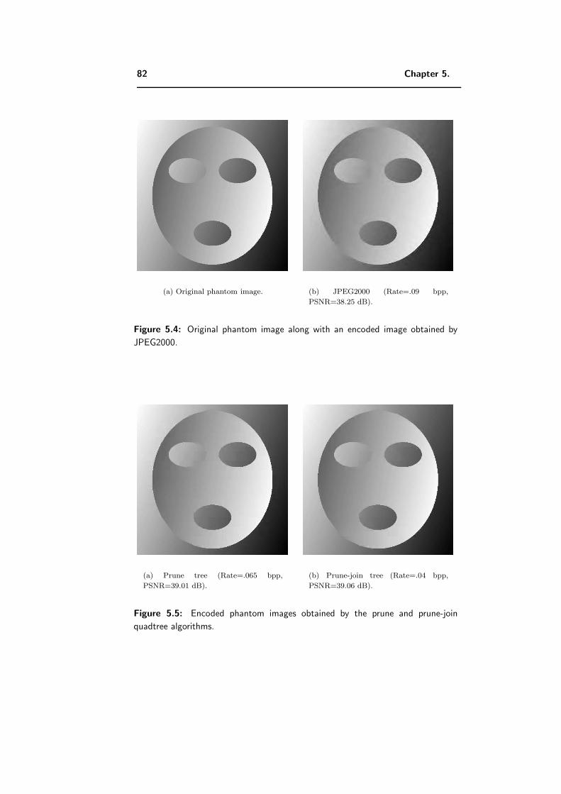
82 Chapter 5.
(a) Original phantom image. (b) JPEG2000 (Rate=.09 bpp,
PSNR=38.25 dB).
Figure 5.4: Original phantom image along with an encoded image obtained by
JPEG2000.
(a) Prune tree (Rate=.065 bpp,
PSNR=39.01 dB).
(b) Prune-join tree (Rate=.04 bpp,
PSNR=39.06 dB).
Figure 5.5: Encoded phantom images obtained by the prune and prune-join
quadtree algorithms.
Chapter 6
New Applications of Tree
Algorithms: Denoising and
Stereo Image Coding
6.1 Introduction
In the previous chapters, we have presented tree segmentation based algo-
rithms and analyzed their compression performance for piecewise smooth sig-
nals/images. In particular, we have shown that the proposed tree based schemes
can not only accurately capture singularities but also efficiently represent the
regular structure separated by these singularities. Since singularities, like edges
in real images, represent one of the most important perceptual information in an
image, their precise modeling is very critical in several signal/image processing
applications, like denoising and computer vision. As we know that the pro-
posed tree algorithms are efficient in exploiting the regularity of singularities as
well as that of the associated smooth regions, these algorithms may show some
potential for image processing applications requiring efficient representation of
singularities.
In this chapter, we focus on two image processing applications, namely de-
noising and stereo image compression, which require to efficiently exploit the
regularity of both the singularities and smooth pieces separated by the singu-
larities. In the next section, we consider the problem of denoising and present a
solution using our tree based algorithm. The key is to treat the denoising prob-
lem as a compression problem at low rates. The intuition is that, at low rates,
the coding scheme captures the dominant (smooth and geometrical) features
only, which basically belong to the original signal. We then present simulation
results and compare our compression based denoising scheme with state of the
art wavelet based denoising scheme in Section 6.2.1. In Section 6.3, we address
83
84 Chapter 6.
the problem of stereo image compression and propose a novel rate-distortion (R-
D) optimized disparity based coding scheme for stereo images. In Section 6.3.2,
we present simulation results for the proposed scheme and compare these results
with the performance of a fixed block size disparity estimation/disparity com-
pensation (DE/DC) based JPEG2000 stereo image coder. Finally, we conclude
with a discussion of further research directions in Section 6.4.
6.2 Denoising Problem
Denoising is a classical problem in estimation theory, which has received an
extensive treatment in the literature [6, 11, 18, 16, 21, 24, 39, 69, 75]. In the
denoising problem, the goal is to estimate the original signal x from an observed
noisy signal y. More formally, consider that the signal x has been corrupted by
the additive white noise z. Thus, the observed signal is
y = x + z.
Our goal is to obtain an estimate, x, of x from y such that the mean squared
error E‖x − x‖2 is minimized. Theoretically, the best estimate is
x = E [x|y] , (6.1)
which is quite difficult to solve in general. This is because Equation (6.1) is
nonlinear, and the conditional probability density px|y required for solving (6.1)
is difficult to calculate. Therefore, one generally settles for the best linear esti-
mate. And this can be obtained by the Wiener filtering approach.1 However,
the Wiener filtering method requires information about the spectra of the noise
and the original signal and it works well only if the underlying signal is smooth.
When the given signal is piecewise smooth, then block based Wiener filtering
can be used. But this approach generally fails to perform well as fixed segmen-
tation cannot capture the real singularities of the underlying piecewise smooth
signal. To overcome the weakness of Wiener filtering, Donoho and Johnstone
proposed the wavelet based denoising scheme in [18]. This wavelet based de-
noising scheme basically projects the noisy signal on the subspace, where the
original signal is supposed to live. This scheme assumes that the noise is low
power and white phenomenon and works as follows
1. Apply the wavelet transform on the noisy signal.
2. Estimate noise strength σ from the high frequency sub-bands.
3. Compute the appropriate threshold t0, e.g., t0 = 3σ.
4. Threshold the wavelet coefficients via hard or soft thresholding scheme.
5. Reconstruct the signal from the thresholded wavelet coefficients. This recon-
structed signal is our denoised signal.
1Wiener filter, that is a linear estimator, is optimal if and only if x and z are jointly
Gaussian processes.
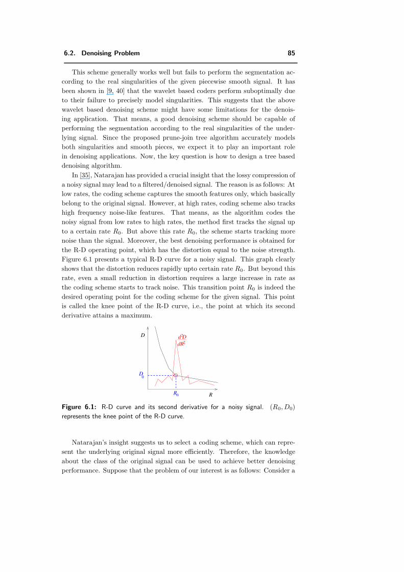
6.2. Denoising Problem 85
This scheme generally works well but fails to perform the segmentation ac-
cording to the real singularities of the given piecewise smooth signal. It has
been shown in [9, 40] that the wavelet based coders perform suboptimally due
to their failure to precisely model singularities. This suggests that the above
wavelet based denoising scheme might have some limitations for the denois-
ing application. That means, a good denoising scheme should be capable of
performing the segmentation according to the real singularities of the under-
lying signal. Since the proposed prune-join tree algorithm accurately models
both singularities and smooth pieces, we expect it to play an important role
in denoising applications. Now, the key question is how to design a tree based
denoising algorithm.
In [35], Natarajan has provided a crucial insight that the lossy compression of
a noisy signal may lead to a filtered/denoised signal. The reason is as follows: At
low rates, the coding scheme captures the smooth features only, which basically
belong to the original signal. However, at high rates, coding scheme also tracks
high frequency noise-like features. That means, as the algorithm codes the
noisy signal from low rates to high rates, the method first tracks the signal up
to a certain rate R0. But above this rate R0, the scheme starts tracking more
noise than the signal. Moreover, the best denoising performance is obtained for
the R-D operating point, which has the distortion equal to the noise strength.
Figure 6.1 presents a typical R-D curve for a noisy signal. This graph clearly
shows that the distortion reduces rapidly upto certain rate R0. But beyond this
rate, even a small reduction in distortion requires a large increase in rate as
the coding scheme starts to track noise. This transition point R0 is indeed the
desired operating point for the coding scheme for the given signal. This point
is called the knee point of the R-D curve, i.e., the point at which its second
derivative attains a maximum.
0R
0D
2dR
R
D 2d D
Figure 6.1: R-D curve and its second derivative for a noisy signal. (R0, D0)
represents the knee point of the R-D curve.
Natarajan’s insight suggests us to select a coding scheme, which can repre-
sent the underlying original signal more efficiently. Therefore, the knowledge
about the class of the original signal can be used to achieve better denoising
performance. Suppose that the problem of our interest is as follows: Consider a
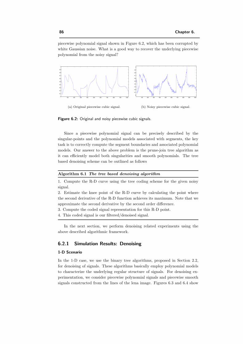
86 Chapter 6.
piecewise polynomial signal shown in Figure 6.2, which has been corrupted by
white Gaussian noise. What is a good way to recover the underlying piecewise
polynomial from the noisy signal?
100 200 300 400 500 600 700 800 900 10000
0.1
0.2
0.3
0.4
0.5
0.6
0.7
0.8
0.9
1
(a) Original piecewise cubic signal.
100 200 300 400 500 600 700 800 900 1000
0
0.1
0.2
0.3
0.4
0.5
0.6
0.7
0.8
0.9
1
(b) Noisy piecewise cubic signal.
Figure 6.2: Original and noisy piecewise cubic signals.
Since a piecewise polynomial signal can be precisely described by the
singular-points and the polynomial models associated with segments, the key
task is to correctly compute the segment boundaries and associated polynomial
models. Our answer to the above problem is the prune-join tree algorithm as
it can efficiently model both singularities and smooth polynomials. The tree
based denoising scheme can be outlined as follows
Algorithm 6.1 The tree based denoising algorithm
1. Compute the R-D curve using the tree coding scheme for the given noisy
signal.
2. Estimate the knee point of the R-D curve by calculating the point where
the second derivative of the R-D function achieves its maximum. Note that we
approximate the second derivative by the second order difference.
3. Compute the coded signal representation for this R-D point.
4. This coded signal is our filtered/denoised signal.
In the next section, we perform denoising related experiments using the
above described algorithmic framework.
6.2.1 Simulation Results: Denoising
1-D Scenario
In the 1-D case, we use the binary tree algorithms, proposed in Section 2.2,
for denoising of signals. These algorithms basically employ polynomial models
to characterize the underlying regular structure of signals. For denoising ex-
perimentation, we consider piecewise polynomial signals and piecewise smooth
signals constructed from the lines of the lena image. Figures 6.3 and 6.4 show
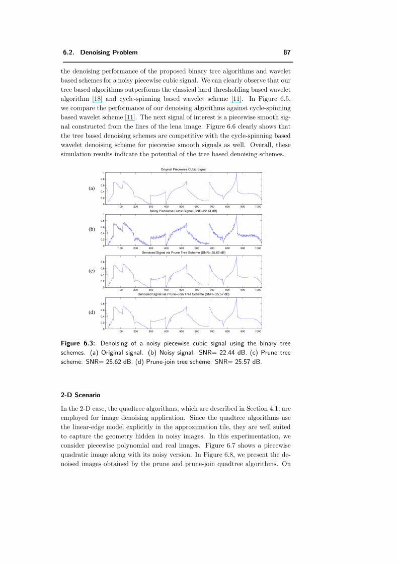
6.2. Denoising Problem 87
the denoising performance of the proposed binary tree algorithms and wavelet
based schemes for a noisy piecewise cubic signal. We can clearly observe that our
tree based algorithms outperforms the classical hard thresholding based wavelet
algorithm [18] and cycle-spinning based wavelet scheme [11]. In Figure 6.5,
we compare the performance of our denoising algorithms against cycle-spinning
based wavelet scheme [11]. The next signal of interest is a piecewise smooth sig-
nal constructed from the lines of the lena image. Figure 6.6 clearly shows that
the tree based denoising schemes are competitive with the cycle-spinning based
wavelet denoising scheme for piecewise smooth signals as well. Overall, these
simulation results indicate the potential of the tree based denoising schemes.
100 200 300 400 500 600 700 800 900 10000
0.2
0.4
0.6
0.8
1Original Piecewise Cubic Signal
100 200 300 400 500 600 700 800 900 10000
0.2
0.4
0.6
0.8
1Noisy Piecewise Cubic Signal (SNR=22.44 dB)
100 200 300 400 500 600 700 800 900 10000
0.2
0.4
0.6
0.8
Denoised Signal via Prune Tree Scheme (SNR= 25.62 dB)
100 200 300 400 500 600 700 800 900 10000
0.2
0.4
0.6
0.8
Denoised Signal via Prune−Join Tree Scheme (SNR= 25.57 dB)
(b)
(c)
(d)
(a)
Figure 6.3: Denoising of a noisy piecewise cubic signal using the binary tree
schemes. (a) Original signal. (b) Noisy signal: SNR= 22.44 dB. (c) Prune tree
scheme: SNR= 25.62 dB. (d) Prune-join tree scheme: SNR= 25.57 dB.
2-D Scenario
In the 2-D case, the quadtree algorithms, which are described in Section 4.1, are
employed for image denoising application. Since the quadtree algorithms use
the linear-edge model explicitly in the approximation tile, they are well suited
to capture the geometry hidden in noisy images. In this experimentation, we
consider piecewise polynomial and real images. Figure 6.7 shows a piecewise
quadratic image along with its noisy version. In Figure 6.8, we present the de-
noised images obtained by the prune and prune-join quadtree algorithms. On
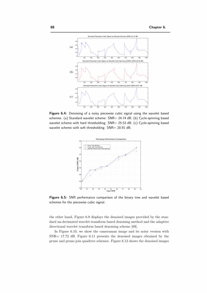
88 Chapter 6.
100 200 300 400 500 600 700 800 900 10000
0.2
0.4
0.6
0.8
Denoised Piecewise Cubic Signal via Wavelet Scheme (SNR=24.74 dB)
100 200 300 400 500 600 700 800 900 1000
0.2
0.4
0.6
0.8
Denoised Piecewise Cubic Signal via Wavelet Cycle Spinning (HARD) (SNR=25.53 dB)
100 200 300 400 500 600 700 800 900 1000
0.2
0.4
0.6
0.8
Denoised Piecewise Cubic Signal via Wavelet Cycle Spinning (Soft) (SNR=20.91 dB)
(a)
(b)
(c)
Figure 6.4: Denoising of a noisy piecewise cubic signal using the wavelet based
schemes. (a) Standard wavelet scheme: SNR= 24.74 dB. (b) Cycle-spinning based
wavelet scheme with hard thresholding: SNR= 25.53 dB. (c) Cycle-spinning based
wavelet scheme with soft thresholding: SNR= 20.91 dB.
20 21 22 23 24 25 26 27 28 29 3024
26
28
30
32
34
36
38Denoising Performance Comparison
Input SNR
Out
put S
NR
(dB
)
Prune Tree SchemePrune−Join Tree SchemeWavelet Scheme with Cycle Spinning
Figure 6.5: SNR performance comparison of the binary tree and wavelet based
schemes for the piecewise cubic signal.
the other hand, Figure 6.9 displays the denoised images provided by the stan-
dard un-decimated wavelet transform based denoising method and the adaptive
directional wavelet transform based denoising scheme [69].
In Figure 6.10, we show the cameraman image and its noisy version with
SNR= 17.72 dB. Figure 6.11 presents the denoised images obtained by the
prune and prune-join quadtree schemes. Figure 6.12 shows the denoised images
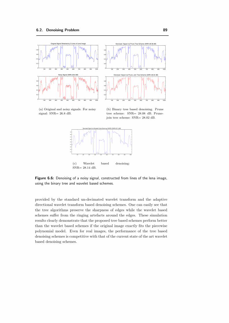
6.2. Denoising Problem 89
100 200 300 400 500 600 700 800 900 10000
0.2
0.4
0.6
0.8
1Original Signal Obtained by 2 Lines of Lena Image
100 200 300 400 500 600 700 800 900 10000
0.2
0.4
0.6
0.8
1Noisy Signal (SNR=26.8 dB)
(a) Original and noisy signals. For noisy
signal: SNR= 26.8 dB.
100 200 300 400 500 600 700 800 900 10000
0.2
0.4
0.6
0.8
1Denoised Signal via Prune Tree Scheme (SNR=28.08 dB)
100 200 300 400 500 600 700 800 900 10000
0.2
0.4
0.6
0.8
1Denoised Signal via Prune−Join Tree Scheme (SNR=28.02 dB)
(b) Binary tree based denoising. Prune
tree scheme: SNR= 28.08 dB. Prune-
join tree scheme: SNR= 28.02 dB.
100 200 300 400 500 600 700 800 900 1000
0.1
0.2
0.3
0.4
0.5
0.6
0.7
0.8
0.9
Denoised Signal via Wavelet Cycle Spinning (HARD) (SNR=28.14 dB)
(c) Wavelet based denoising:
SNR= 28.14 dB.
Figure 6.6: Denoising of a noisy signal, constructed from lines of the lena image,
using the binary tree and wavelet based schemes.
provided by the standard un-decimated wavelet transform and the adaptive
directional wavelet transform based denoising schemes. One can easily see that
the tree algorithms preserve the sharpness of edges while the wavelet based
schemes suffer from the ringing artefacts around the edges. These simulation
results clearly demonstrate that the proposed tree based schemes perform better
than the wavelet based schemes if the original image exactly fits the piecewise
polynomial model. Even for real images, the performance of the tree based
denoising schemes is competitive with that of the current state of the art wavelet
based denoising schemes.
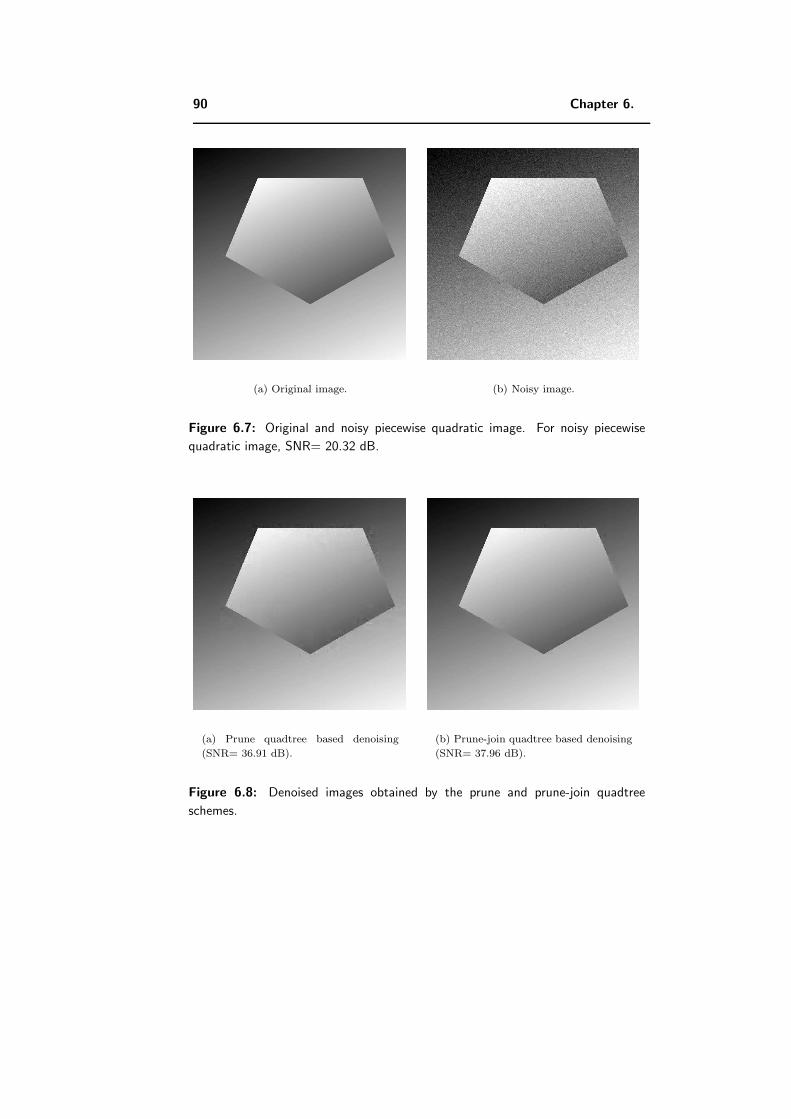
90 Chapter 6.
(a) Original image. (b) Noisy image.
Figure 6.7: Original and noisy piecewise quadratic image. For noisy piecewise
quadratic image, SNR= 20.32 dB.
(a) Prune quadtree based denoising
(SNR= 36.91 dB).
(b) Prune-join quadtree based denoising
(SNR= 37.96 dB).
Figure 6.8: Denoised images obtained by the prune and prune-join quadtree
schemes.
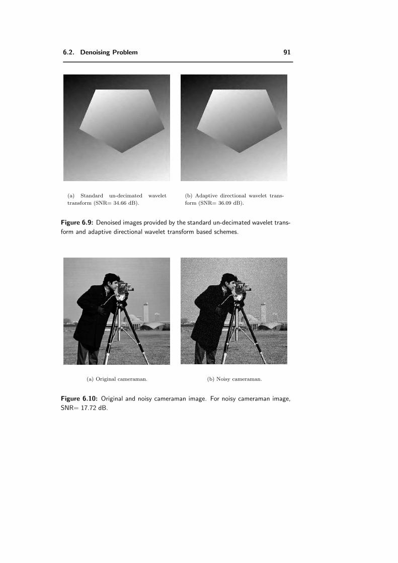
6.2. Denoising Problem 91
(a) Standard un-decimated wavelet
transform (SNR= 34.66 dB).
(b) Adaptive directional wavelet trans-
form (SNR= 36.09 dB).
Figure 6.9: Denoised images provided by the standard un-decimated wavelet trans-
form and adaptive directional wavelet transform based schemes.
(a) Original cameraman. (b) Noisy cameraman.
Figure 6.10: Original and noisy cameraman image. For noisy cameraman image,
SNR= 17.72 dB.
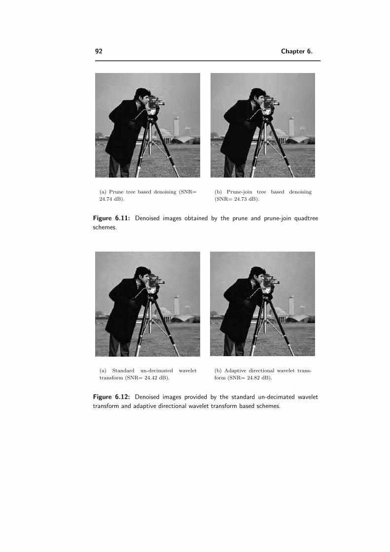
92 Chapter 6.
(a) Prune tree based denoising (SNR=
24.74 dB).
(b) Prune-join tree based denoising
(SNR= 24.73 dB).
Figure 6.11: Denoised images obtained by the prune and prune-join quadtree
schemes.
(a) Standard un-decimated wavelet
transform (SNR= 24.42 dB).
(b) Adaptive directional wavelet trans-
form (SNR= 24.82 dB).
Figure 6.12: Denoised images provided by the standard un-decimated wavelet
transform and adaptive directional wavelet transform based schemes.
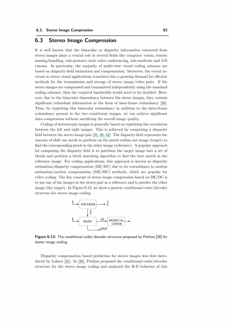
6.3. Stereo Image Compression 93
6.3 Stereo Image Compression
It is well known that the binocular or disparity information extracted from
stereo images plays a crucial role in several fields like computer vision, remote
sensing/handling, tele-presence style video conferencing, tele-medicine and 3-D
cinema. In particular, the majority of multi-view visual coding schemes are
based on disparity-field estimation and compensation. Moreover, the recent in-
crease in stereo visual applications translates into a growing demand for efficient
methods for the transmission and storage of stereo image/video pairs. If the
stereo images are compressed and transmitted independently using the standard
coding schemes, then the required bandwidth would need to be doubled. How-
ever, due to the binocular dependency between the stereo images, they contain
significant redundant information in the form of inter-frame redundancy [38].
Thus, by exploiting this binocular redundancy in addition to the intra-frame
redundancy present in the two constituent images, we can achieve significant
data compression without sacrificing the overall image quality.
Coding of stereoscopic images is generally based on exploiting the correlation
between the left and right images. This is achieved by computing a disparity
field between the stereo image pair [31, 38, 42]. The disparity field represents the
amount of shift one needs to perform on the pixels within one image (target) to
find the corresponding pixels in the other image (reference). A popular approach
for computing the disparity field is to partition the target image into a set of
blocks and perform a block matching algorithm to find the best match in the
reference image. For coding applications, this approach is known as disparity
estimation/disparity compensation (DE/DC) due to its resemblance to motion
estimation/motion compensation (ME/MC) methods, which are popular for
video coding. The key concept of stereo image compression based on DE/DC is
to use one of the images in the stereo pair as a reference and to predict the other
image (the target). In Figure 6.13, we show a generic conditional coder/decoder
structure for stereo image coding.
I∆CODER
RESIDUAL
DVF
2
ENCODER
DE/DC
1I
2I
^1I
^1I
Figure 6.13: The conditional coder/decoder structure proposed by Perkins [38] for
stereo image coding.
Disparity compensation based prediction for stereo images was first intro-
duced by Lukacs [31]. In [38], Perkins proposed the conditional coder/decoder
structure for the stereo image coding and analyzed the R-D behavior of this

94 Chapter 6.
structure. Aydinoglu et al. presented a coding scheme which combines disparity
compensation and transform coding of the residual image in the single frame-
work using an adaptive incomplete transform [1]. Hierarchical block matching
algorithms have been used to generate a more homogeneous disparity fields that
lead to better coding efficiency [49, 63].
In [4], a novel scheme is presented for the efficient exploitation of the ze-
rotree algorithm in stereo image coding applications. Disparity field estimation
based on low level features, such as edges, and on model/object based meth-
ods have also been used [58]. In [63], a feature/object based DE/DC scheme
is proposed. This scheme determines a set of objects/features in both images
and seeks correspondence between the two sets. Jiang [25] proposed a hybrid
approach between block and object based schemes for the efficient coding of
stereo pairs. In [73], overlapped block disparity compensation with adaptive
search windows is presented. In [34], Moellenhoff et al. analyzed the proper-
ties of disparity compensated residual images and proposed transform domain
coding methods for improved coding of residual images. Other efforts on stereo
coding have focused on optimal rate-distortion based algorithms for block de-
pendent quantization [72] and motion/disparity field estimation [64].
Our goal is to develop a compression algorithm, which performs the dis-
parity dependent segmentation of stereo images in an R-D framework. We
employ a generalized quadtree decomposition based DE/DC. This scheme fur-
ther performs the joint coding of the disparity information and the residual
image obtained by the disparity compensation in an R-D optimal sense. In the
next section, we describe the proposed disparity dependent segmentation based
coding scheme for stereo images. We then present some simulation results in
Section 6.3.2.
6.3.1 Disparity Dependent Segmentation Based Stereo Image
Coding Algorithm
The generic structure of a stereo image coding scheme is as follows: First encode
one of the images of the stereo pair as reference, then estimate the disparity in-
formation between blocks in the target and encoded reference images and code
the disparity information and the residual image obtained by subtracting the
disparity compensated target image from the original image. The disparity
compensated/predicted target image is obtained by using the encoded refer-
ence image and the disparity map. Thus, our scheme employs the closed loop
methodology for obtaining the predicted target image.
The main novelty of our stereo image coding scheme is that it performs
the disparity dependent quadtree segmentation in an R-D framework.2 This
disparity dependent segmentation based stereo image coding scheme can be
described as follows:
2Mean squared error (MSE) is used as a distortion measure.
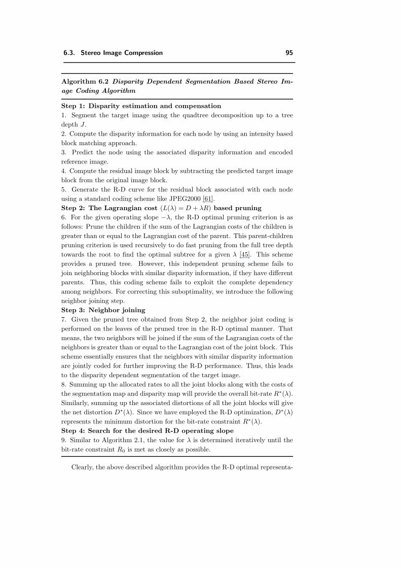
6.3. Stereo Image Compression 95
Algorithm 6.2 Disparity Dependent Segmentation Based Stereo Im-
age Coding Algorithm
Step 1: Disparity estimation and compensation
1. Segment the target image using the quadtree decomposition up to a tree
depth J .
2. Compute the disparity information for each node by using an intensity based
block matching approach.
3. Predict the node using the associated disparity information and encoded
reference image.
4. Compute the residual image block by subtracting the predicted target image
block from the original image block.
5. Generate the R-D curve for the residual block associated with each node
using a standard coding scheme like JPEG2000 [61].
Step 2: The Lagrangian cost (L(λ) = D + λR) based pruning
6. For the given operating slope −λ, the R-D optimal pruning criterion is as
follows: Prune the children if the sum of the Lagrangian costs of the children is
greater than or equal to the Lagrangian cost of the parent. This parent-children
pruning criterion is used recursively to do fast pruning from the full tree depth
towards the root to find the optimal subtree for a given λ [45]. This scheme
provides a pruned tree. However, this independent pruning scheme fails to
join neighboring blocks with similar disparity information, if they have different
parents. Thus, this coding scheme fails to exploit the complete dependency
among neighbors. For correcting this suboptimality, we introduce the following
neighbor joining step.
Step 3: Neighbor joining
7. Given the pruned tree obtained from Step 2, the neighbor joint coding is
performed on the leaves of the pruned tree in the R-D optimal manner. That
means, the two neighbors will be joined if the sum of the Lagrangian costs of the
neighbors is greater than or equal to the Lagrangian cost of the joint block. This
scheme essentially ensures that the neighbors with similar disparity information
are jointly coded for further improving the R-D performance. Thus, this leads
to the disparity dependent segmentation of the target image.
8. Summing up the allocated rates to all the joint blocks along with the costs of
the segmentation map and disparity map will provide the overall bit-rate R∗(λ).
Similarly, summing up the associated distortions of all the joint blocks will give
the net distortion D∗(λ). Since we have employed the R-D optimization, D∗(λ)
represents the minimum distortion for the bit-rate constraint R∗(λ).
Step 4: Search for the desired R-D operating slope
9. Similar to Algorithm 2.1, the value for λ is determined iteratively until the
bit-rate constraint R0 is met as closely as possible.
Clearly, the above described algorithm provides the R-D optimal representa-
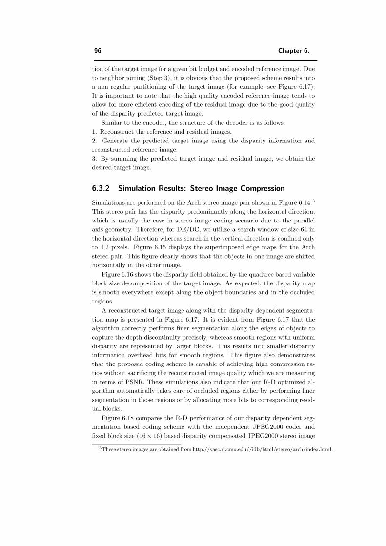
96 Chapter 6.
tion of the target image for a given bit budget and encoded reference image. Due
to neighbor joining (Step 3), it is obvious that the proposed scheme results into
a non regular partitioning of the target image (for example, see Figure 6.17).
It is important to note that the high quality encoded reference image tends to
allow for more efficient encoding of the residual image due to the good quality
of the disparity predicted target image.
Similar to the encoder, the structure of the decoder is as follows:
1. Reconstruct the reference and residual images.
2. Generate the predicted target image using the disparity information and
reconstructed reference image.
3. By summing the predicted target image and residual image, we obtain the
desired target image.
6.3.2 Simulation Results: Stereo Image Compression
Simulations are performed on the Arch stereo image pair shown in Figure 6.14.3
This stereo pair has the disparity predominantly along the horizontal direction,
which is usually the case in stereo image coding scenario due to the parallel
axis geometry. Therefore, for DE/DC, we utilize a search window of size 64 in
the horizontal direction whereas search in the vertical direction is confined only
to ±2 pixels. Figure 6.15 displays the superimposed edge maps for the Arch
stereo pair. This figure clearly shows that the objects in one image are shifted
horizontally in the other image.
Figure 6.16 shows the disparity field obtained by the quadtree based variable
block size decomposition of the target image. As expected, the disparity map
is smooth everywhere except along the object boundaries and in the occluded
regions.
A reconstructed target image along with the disparity dependent segmenta-
tion map is presented in Figure 6.17. It is evident from Figure 6.17 that the
algorithm correctly performs finer segmentation along the edges of objects to
capture the depth discontinuity precisely, whereas smooth regions with uniform
disparity are represented by larger blocks. This results into smaller disparity
information overhead bits for smooth regions. This figure also demonstrates
that the proposed coding scheme is capable of achieving high compression ra-
tios without sacrificing the reconstructed image quality which we are measuring
in terms of PSNR. These simulations also indicate that our R-D optimized al-
gorithm automatically takes care of occluded regions either by performing finer
segmentation in those regions or by allocating more bits to corresponding resid-
ual blocks.
Figure 6.18 compares the R-D performance of our disparity dependent seg-
mentation based coding scheme with the independent JPEG2000 coder and
fixed block size (16× 16) based disparity compensated JPEG2000 stereo image
3These stereo images are obtained from http://vasc.ri.cmu.edu//idb/html/stereo/arch/index.html.
6.4. Discussion 97
coder. This R-D performance comparison clearly shows the superiority of the
proposed algorithm over the other two algorithms.
(a) Reference image. (b) Target image.
Figure 6.14: Original Arch stereo pair.
Figure 6.15: Superimposed edge-maps for the Arch stereo pair.
6.4 Discussion
In this chapter, we have addressed two interesting problems, namely denois-
ing and stereo image compression, using tree structured segmentation. In Sec-
tion 6.2, we have presented a tree based denoising scheme, which can efficiently
extract geometrical structures from noisy images. Simulation results shown in
Section 6.2.1 clearly demonstrate that our scheme is competitive with the cur-
rent state of the art wavelet based schemes. Moreover, it is also evident from
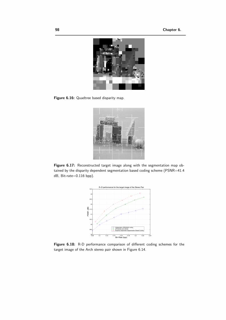
98 Chapter 6.
Figure 6.16: Quadtree based disparity map.
Figure 6.17: Reconstructed target image along with the segmentation map ob-
tained by the disparity dependent segmentation based coding scheme (PSNR=41.4
dB, Bit-rate=0.116 bpp).
0.08 0.1 0.12 0.14 0.16 0.18 0.2 0.22 0.2439
39.5
40
40.5
41
41.5
42
42.5
43
43.5R−D performance for the target image of the Stereo Pair
Bit−Rate (bpp)
PS
NR
(dB
)
Independent JPEG2000 codingJPEG2000 with DE/DCDisparity Dependent Segmentation Based Coding
Figure 6.18: R-D performance comparison of different coding schemes for the
target image of the Arch stereo pair shown in Figure 6.14.

6.4. Discussion 99
Figures 6.8 and 6.11 that the proposed scheme captures geometrical features,
like edges, of images more precisely compared to wavelet based schemes. Our
on-going work aims to extend the present algorithm such that it can also dis-
tinguish the texture present in images from random noise for further improving
the visual quality of denoised images.
In Section 6.3.1, we have developed an R-D optimized disparity dependent
segmentation based stereo image coding scheme. This new scheme performs
the joint coding of disparity information and the residual image to achieve
the improved R-D performance. Experimental results presented in Figure 6.18
also show that the proposed scheme outperforms the disparity compensated
JPEG2000 stereo coder by about 0.5 dB. Since our scheme employs a quadtree
based decomposition, this scheme is computationally efficient as well. Our on-
going research effort is to extend this stereo image coding scheme to multi-view
image and stereo video coding scenarios. We would also like to investigate fea-
ture/object based DE/DC scheme in the framework of the proposed algorithm.

100 Chapter 6.
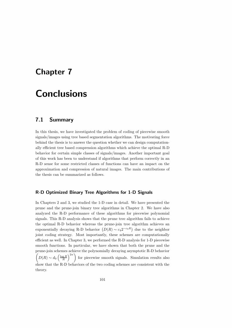
Chapter 7
Conclusions
7.1 Summary
In this thesis, we have investigated the problem of coding of piecewise smooth
signals/images using tree based segmentation algorithms. The motivating force
behind the thesis is to answer the question whether we can design computation-
ally efficient tree based compression algorithms which achieve the optimal R-D
behavior for certain simple classes of signals/images. Another important goal
of this work has been to understand if algorithms that perform correctly in an
R-D sense for some restricted classes of functions can have an impact on the
approximation and compression of natural images. The main contributions of
the thesis can be summarized as follows.
R-D Optimized Binary Tree Algorithms for 1-D Signals
In Chapters 2 and 3, we studied the 1-D case in detail. We have presented the
prune and the prune-join binary tree algorithms in Chapter 2. We have also
analyzed the R-D performance of these algorithms for piecewise polynomial
signals. This R-D analysis shows that the prune tree algorithm fails to achieve
the optimal R-D behavior whereas the prune-join tree algorithm achieves an
exponentially decaying R-D behavior(D(R) ∼ c42
−c5R)
due to the neighbor
joint coding strategy. Most importantly, these schemes are computationally
efficient as well. In Chapter 3, we performed the R-D analysis for 1-D piecewise
smooth functions. In particular, we have shown that both the prune and the
prune-join schemes achieve the polynomially decaying asymptotic R-D behavior(D(R) ∼ d0
(log R
R
)2α)
for piecewise smooth signals. Simulation results also
show that the R-D behaviors of the two coding schemes are consistent with the
theory.
101
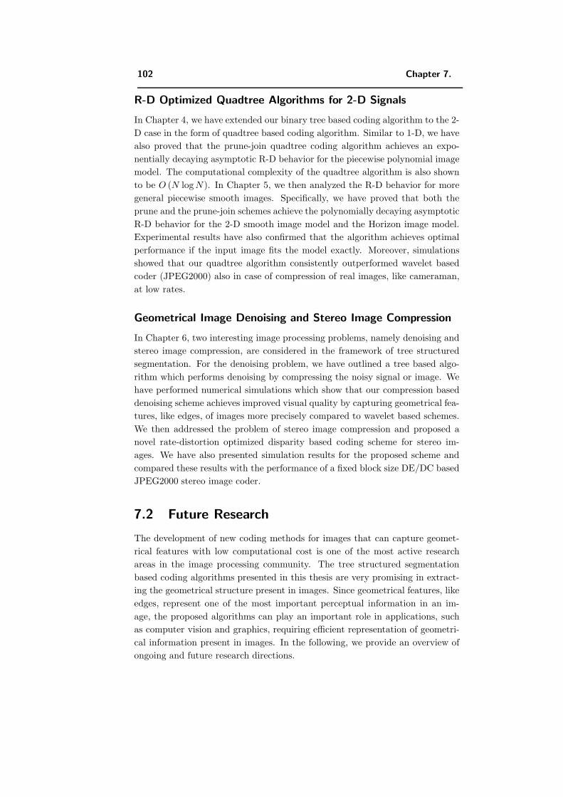
102 Chapter 7.
R-D Optimized Quadtree Algorithms for 2-D Signals
In Chapter 4, we have extended our binary tree based coding algorithm to the 2-
D case in the form of quadtree based coding algorithm. Similar to 1-D, we have
also proved that the prune-join quadtree coding algorithm achieves an expo-
nentially decaying asymptotic R-D behavior for the piecewise polynomial image
model. The computational complexity of the quadtree algorithm is also shown
to be O (N log N). In Chapter 5, we then analyzed the R-D behavior for more
general piecewise smooth images. Specifically, we have proved that both the
prune and the prune-join schemes achieve the polynomially decaying asymptotic
R-D behavior for the 2-D smooth image model and the Horizon image model.
Experimental results have also confirmed that the algorithm achieves optimal
performance if the input image fits the model exactly. Moreover, simulations
showed that our quadtree algorithm consistently outperformed wavelet based
coder (JPEG2000) also in case of compression of real images, like cameraman,
at low rates.
Geometrical Image Denoising and Stereo Image Compression
In Chapter 6, two interesting image processing problems, namely denoising and
stereo image compression, are considered in the framework of tree structured
segmentation. For the denoising problem, we have outlined a tree based algo-
rithm which performs denoising by compressing the noisy signal or image. We
have performed numerical simulations which show that our compression based
denoising scheme achieves improved visual quality by capturing geometrical fea-
tures, like edges, of images more precisely compared to wavelet based schemes.
We then addressed the problem of stereo image compression and proposed a
novel rate-distortion optimized disparity based coding scheme for stereo im-
ages. We have also presented simulation results for the proposed scheme and
compared these results with the performance of a fixed block size DE/DC based
JPEG2000 stereo image coder.
7.2 Future Research
The development of new coding methods for images that can capture geomet-
rical features with low computational cost is one of the most active research
areas in the image processing community. The tree structured segmentation
based coding algorithms presented in this thesis are very promising in extract-
ing the geometrical structure present in images. Since geometrical features, like
edges, represent one of the most important perceptual information in an im-
age, the proposed algorithms can play an important role in applications, such
as computer vision and graphics, requiring efficient representation of geometri-
cal information present in images. In the following, we provide an overview of
ongoing and future research directions.
7.2. Future Research 103
Search for Globally Optimal Solution
Consider a discontinuous function f(t) which is generated by multiplying a
polynomial p(t) with an on-off square pulse train. This function is either zero
or characterized by only one polynomial p(t). An oracle based scheme observes
this fact and codes the signal accordingly to obtain the globally optimal solution.
However, our tree based scheme, which is presently able to exploit the neighbor
similarity only, cannot observe this phenomenon hidden in the signal. So clearly
the tree scheme cannot perform as well as the oracle method. However, since
the generated signal has only finite degrees of freedom, the tree scheme still
achieves an exponentially decaying R-D behavior. But the rate of decay is
smaller in comparison to that of the oracle method. An interesting direction of
work would be to incorporate the concept of global similarity in the framework
of the tree algorithm so that the tree scheme can match the performance of the
oracle method for the above described synthetic signals as well.
Texture Modeling
The main focus of this thesis remains the efficient representation of smooth sur-
faces and smooth edges separating the smooth regions without much attention
to the proper modeling/coding of texture present in natural images. Since nat-
ural images can be more accurately modeled as a sum of 2-D piecewise smooth
function and texture [24], we need to incorporate efficient texture modeling to
achieve improved performance for natural images at high rates. It is well known
that wavelets can model texture better than piecewise polynomials. Thus, the
quadtree scheme should model tree nodes with texture using wavelets and tree
nodes with geometrical information using a geometrical tile composed of two
2-D polynomials separated by a linear edge. In this way, this new scheme will
enjoy the best of both wavelets modeling and geometrical modeling and hope-
fully achieve a better R-D performance.
Multi-view Image and Stereo Video Coding
For the problem of stereo image compression, we have seen that the proposed
disparity dependent segmentation based scheme outperforms JPEG2000 based
stereo coder. Therefore, it is of interest to extend this stereo image coding
scheme to multi-view image and stereo video coding scenarios. In particular,
using feature/object based DE/DC and ME/MC schemes in the framework of
the proposed algorithm may provide improved performance.
Distributed Stereo Image Coding
Another interesting problem setup is the distributed coding scenario for stereo
images. For instance, consider an electronic surveillance system where the two

104 Chapter 7.
cameras are viewing the same scene and sending the images to the central se-
curity unit for further processing. In this setup, communication between the
two encoders is not allowed due to some constraints such as power constraint.
However, both encoders have the information about the correlation structure of
the observed entities. In this scenario, an open issue is to understand whether
we can design distributed stereo coding schemes which can perform as well as
the traditional stereo coding schemes.
Bibliography
[1] H. Aydinoglu and H. Hayes, “Stereo image coding: A projection approach,”
IEEE Trans. Image Proc., vol. 7, pp. 506-516, Apr. 1998.
[2] D. H. Ballard and C. M. Brown, Computer Vision, Prentice-Hall, Englewood
Cliffs NJ, 1982.
[3] L. Balmelli, M. Vetterli and T. Liebling, “Mesh optimization using global
error with application to geometry simplification,” Graphical Models 64,
230-257 (2002), Special Issue on Processing of Large Polygonal Meshes, Aca-
demic Press.
[4] N. V. Boulgouris and M. G. Strintzis, “A family of wavelet-based stereo
image coders,” IEEE Trans. Circuits Syst. Video Tech., vol. 12, no. 10,
pp. 898-903, Oct. 2002.
[5] E. J. Candes and D. L. Donoho, “Curvelets- a surprisingly effective non-
adaptive representation for objects with edges,” in Curve and Surface Fit-
ting, A. Cohen, C. Rabut, and L. L. Schumaker, Eds., Saint-Malo, 1999,
Vanderbilt University Press.
[6] S. G. Chang, B. Yu, M. Vetterli, “Spatially adaptive image wavelet thresh-
olding with context modeling for image denoising,” IEEE Trans. on Image
Proc. 9(9):1522-1531, Sep. 2000
[7] S. G. Chang, B. Yu, M. Vetterli, “Wavelet thresholding for multiple noisy
image copies,” IEEE Trans. Image Proc., 9(9):1631-1635, Sep. 2000
[8] P. A. Chou, T. Lookabaugh and R.M. Gray, “Optimal pruning with applica-
tions to tree structured source coding and modeling,” IEEE Trans. Inform.
Th., vol. IT-35, pp. 299-315, Mar. 1989.
[9] A. Cohen, I. Daubechies, O.G. Guleryuz and M.T. Orchard, “On the im-
portance of combining wavelet-based nonlinear approximation with coding
strategies,” IEEE Trans. Inform. Th.,, vol. 48, pp. 1895 -1921, July 2002.
[10] A.Cohen and B.Matei, “Compact representations of images by edge
adapted multiscale transforms,” in Proc. IEEE Int. Conf. on Image
Proc.(ICIP), Thessaloniki, Greece, Oct. 2001.
105
106 BIBLIOGRAPHY
[11] R.R. Coifman and D.L. Donoho, “Translation invariant denoising,” Tech.
Rep., Department of Statistics, Stanford University, May 1995.
[12] T.M. Cover and J.A. Thomas, Elements of Information Theory, John Wiley
and Sons, 1991.
[13] S. Dekel, D. Leviatan and M. Sharir, “On bivariate smoothness spaces
associated with nonlinear approximation,” Constructive Approximation (to
appear).
[14] M.N. Do, P. L. Dragotti, R. Shukla and M. Vetterli, “On the compression
of two dimensional piecewise smooth functions,” in Proc. IEEE Int. Conf.
on Image Proc., Thessaloniki, Greece, Oct. 2001.
[15] M. N. Do and M. Vetterli, “Contourlets: Beyond Wavelets,” J. Stoeckler
and G. V. Welland eds., Academic Press, 2003.
[16] D.L. Donoho, “Wedgelets: Nearly minimax estimation of edges”, Annals
of Statistics, 27(3):859-897, 1999.
[17] D.L. Donoho and X. Huo, “Beamlets and multiscale image analysis,” Tech.
Rep., Department of Statistics, Stanford University, 2001.
[18] D.L. Donoho and I.M. Johnstone, “Ideal Spatial adaptation via wavele t
shrinkage,” Biometrika, 81:425-455, Dec. 1994.
[19] D.L. Donoho, M. Vetterli, R.A. DeVore, and I. Daubechies, “Data com-
pression and harmonic analysis,” IEEE Trans. Inform. Th., vol. 44, no. 6,
pp. 2435-2476, Oct. 1998.
[20] P. L. Dragotti, Wavelet Footprints and Frames for Signal Processing and
Communications, PhD Thesis, Department of Communication Systems,
Swiss Federal Institute of Technology Lausanne, April 2002.
[21] P. L. Dragotti and M. Vetterli, “Wavelet footprints: theory, algorithms
and applications,” IEEE Trans. Signal Proc., vol. 51(5), pp. 1306-1323, May
2003.
[22] V. K. Goyal, “Theoretical foundations of transform coding,” IEEE SP
Mag., vol. 18, no. 5, pp. 9-21, Sep. 2001.
[23] J. J. Y. Huang and P. M. Schultheiss, “Block quantization of correlated
Gaussian random variables,” IEEE Trans. Comm., vol. 11, pp. 289-296,
Sep. 1963.
[24] A.K. Jain, Fundamentals of Digital Image Processing, Prentice Hall Inc.,
1989.
BIBLIOGRAPHY 107
[25] J. Jiang and E. A. Edirisinghe, “A hybrid scheme for low bit-rate coding
of stereo images,” IEEE Trans. Image Proc., vol. 11, no. 2, pp. 123-134,
Feb. 2002.
[26] A. P. Korostelev and A. B. Tsybakov, Minimax theory of image reconstruc-
tion, Springer-Verlag, New York, 1993.
[27] F. Labonte, C. T. Le Dinh, J. Faubert, and P. Cohen, “Spatiotemporal
spectral coding of stereo image sequences,” IEEE Trans. Circuits, Syst.,
Video Tech., vol. 9, pp. 144-155, Feb. 1999.
[28] W. S. Lee, “Tiling and adaptive image compression,” IEEE Trans. on In-
form. Th., vol. 46, no. 5, Aug. 2000.
[29] R. Leonardi and M. Kunt, “Adaptive split and merge for image analysis
and coding,” Proc. SPIE, vol. 594, 1985.
[30] T. Lookabaugh and R.M. Gray, “High resolution quantization theory and
the vector quantizer advantage,” IEEE Trans. Inform. Th., vol. 35, pp.
1020-1033, Sep. 1989.
[31] M. E. Lukacs, “Predictive coding of multi-viewpoint image sets,” in Proc.
ICASSP, Oct. 1986, pp. 521-524.
[32] S. Mallat, A Wavelet Tour of Signal Processing, Academic Press, San
Diego, CA, USA, 1997.
[33] S. Mallat and W.L. Hwang, “Singularity detection and processing with
wavelets,” IEEE Trans. on Inform. Th., 38:617-643, March 1992.
[34] M. S. Moellenhoff and M.W. Maier, “Transform coding of stereo image
residuals,” IEEE Trans. Image Proc., vol. 7, pp. 804-812, June 1998.
[35] B. K. Natarajan, “Filtering Random Noise from Deterministic Signals via
Data Compression,” IEEE Trans. Signal Proc., vol. 43(11), pp. 2595-2605,
Nov. 1995.
[36] W.B. Pennebaker and J.L.Mitchell, JPEG Still Image Data Compression
Standard, Van Nostrand Reinhold, New York, 1993.
[37] E. Le Pennec and S. Mallat, “Bandelet representation for image compres-
sion,” in Proc. IEEE Int. Conf. on Image Proc.(ICIP), Thessaloniki, Greece,
Oct. 2001.
[38] M. G. Perkins, “Data compression of stereo pairs,” IEEE Trans. Comm.,
vol. 40, pp. 684-696, Apr. 1992.
[39] J. Portilla, V. Strela, M. J. Wainwright, and E. P. Simoncelli, “Image
denoising using gaussian scale mixtures in the wavelet domain,” IEEE Trans.
Image Proc., vol. 12(11), pp. 1338 - 1351, Nov. 2003.
108 BIBLIOGRAPHY
[40] P. Prandoni and M.Vetterli, “Approximation and compression of piecewise
smooth functions,” Phil. Trans. Royal Society London, vol. 357, no. 1760,
pp. 2573-2591, Sep. 1999.
[41] P. Prandoni, Optimal Segmentation Techniques for Piecewise Stationary
Signals, PhD Thesis, Swiss Federal Institute of Technology, Lausanne,
Switzerland, 1999.
[42] A. Puri, R. V. Kollarits, and B. G. Haskell, “Basics of stereoscopic video,
new compression results with MPEG-2 and a proposal for MPEG-4,” Jour.
Signal Proc. Image Comm., vol. 10, pp. 201-234, 1997.
[43] M. Rabbani and P. W. Jones, Digital Image Compression Techniques,
Bellingham, WA, SPIE Press, 1991.
[44] H. Radha, M. Vetterli and R. Leonardi, “Image compression using binary
space partitioning trees,” IEEE Trans. Image Proc., vol. 5, no. 12, pp. 1610-
1624, Dec. 1996.
[45] K.Ramchandran and M.Vetterli, “Best wavelet packet bases in a rate dis-
tortion sense,” IEEE Trans. Image Proc., vol. 2, no. 2, pp. 160-175, April
1993.
[46] E.A.Riskin, “Optimal bit allocation via the generalized BFOS algorithm,”
IEEE Trans. Inform. Th., vol. 37, pp. 299-315, Mar. 1991.
[47] J. K. Romberg, H. Choi, and R. G. Baraniuk, “Bayesian tree-structured
image modeling using wavelet domain hidden markov models,” IEEE Trans.
Image Proc., vol. 10, pp. 1056-1068, no. 7, July 2001.
[48] A. Segall, “ Bit allocation and encoding for vector sources,” IEEE Trans.
Inform. Th., vol. IT-22, pp. 162-169, Mar. 1976.
[49] S. Sethuramam, M. W. Siegel, and A. G. Jordan, “A multi-resolution frame-
work for stereoscopic image sequence compression,” in Proc. ICIP-95, vol.
2, pp. 361-365.
[50] Y. Shoham and A. Gersho, “ Efficient bit allocation for an arbitrary set
of quantizers,” IEEE Trans. Acoust. Speech Signal Proc., vol. 36, pp. 1445-
1453, Sep. 1988.
[51] R. Shukla, M.N. Do, P. L. Dragotti and M. Vetterli, “Rate-distortion opti-
mal tree based coding algorithms for piecewise polynomials,” in Proc. IEEE
Int. Symp. on Information Theory, Switzerland, July 2002.
[52] R. Shukla, P. L. Dragotti, M.N. Do and M. Vetterli, “Improved quadtree
algorithm based on joint coding for piecewise smooth image compression,”
in Proc. IEEE Int. Conf. on Multimedia, Switzerland, Aug. 2002.
BIBLIOGRAPHY 109
[53] R. Shukla, P. L. Dragotti, M.N. Do and M. Vetterli, “Rate-distortion op-
timized tree based coding algorithms,” Proc. of IEEE Int. Workshop on
Information Th., India, October 2002.
[54] R. Shukla, P. L. Dragotti, M.N. Do and M. Vetterli, “Rate-distortion opti-
mized tree structured compression algorithms for piecewise smooth images,”
accepted to IEEE Trans. Image Proc., Mar. 2004.
[55] Rahul Shukla, Hayder Radha and M.Vetterli, “Disparity Dependent Seg-
mentation Based Stereo Image Coding,” in Proc. IEEE Int. Conf. on Image
Proc., Barcelona, Sep. 2003.
[56] Rahul Shukla and M.Vetterli, “Geometrical Image Denoising Using
Quadtree Segmentation,” submitted to IEEE Int. Conf. on Image Proc.,
Singapore, Oct. 2004.
[57] “Transform Coding: Past, Present and Future,” Special Issue, IEEE SP
Mag., vol. 18, no. 5, Sep. 2001.
[58] M. G. Strintzis and S. Malassiotis, “Object-based coding of stereoscopic and
3D image sequences: A review,” IEEE Signal Proc. Mag., vol. 16, pp. 14-29,
May 1999.
[59] P. Strobach, “Quadtree structured recursive plane decomposition coding of
images,” IEEE Trans. Signal Proc., vol. 39, pp. 1380-1397, June 1991.
[60] G.J. Sullivan and R.L. Baker, “Efficient quadtree coding of images and
video,” IEEE Trans. Image Proc., vol. 3, no. 3, pp. 327-331, May 1994.
[61] D. Taubman and M. Marcellin, JPEG2000: Image Compression Funda-
mentals, Standards and Practice, Kluwer Academic Publishers, Dordrecht,
2001.
[62] H. Triebel, Interpolation Theory, Function Spaces, Differential Operators,
North-Holland, Amsterdam, 1978.
[63] D. Tzovaras, N. Grammalidis, and M. G. Strintzis, “Object-based coding
of stereo image sequences using joint 3D motion/disparity compensation,”
IEEE Trans. Circuits Syst. Video Tech., vol. 7, pp. 312-327, Apr. 1997.
[64] D. Tzovaras and M. G. Strintzis, “Motion and disparity field estimation
using rate-distortion optimization,” IEEE Trans. Circuits Syst. Video Tech.,
vol. 8, pp. 171-180, Apr. 1998.
[65] D.J. Vaisey and A. Gersho, “Image coding with variable block size segmen-
tation,” IEEE Trans. Signal Proc., vol. SP-40, pp. 2040-2060, Aug.1992.
[66] R. M. F. Ventura, L. Granai and P. Vandergheynst, “R-D analysis of adap-
tive edge representations,” in Proc. of IEEE MMSP, Dec. 2002.
110 BIBLIOGRAPHY
[67] M.Vetterli, “Wavelets, approximation and compression,” IEEE SP Mag.,
vol. 18, no. 5, pp. 59-73, Sep. 2001.
[68] M.Vetterli and J. Kovacevic, Wavelets and Subband Coding, Prentice Hall,
Englewood Cliffs, NJ, 1995.
[69] V. Velisavljevic, B. Beferull-Lozano, M. Vetterli, and P. L. Dragotti, “Dis-
crete Multi-directional Wavelet Bases,” IEEE Int. Conf. on Image Proc. ,
Barcelona, Sep. 2003.
[70] M. Wakin, J. Romberg, H. Choi, and R. Baraniuk, “Rate-distortion op-
timized image compression using wedgelets,” IEEE Int. Conf. on Image
Proc., USA, Sep. 2002.
[71] R. Willett and R. Nowak, “Platelets: a multiscale approach for recovering
edges and surfaces in photon-limited medical imaging,” IEEE Trans. on
Medical Imaging, Vol. 22, no. 3, pp. 332 -350, March 2003.
[72] W. Woo and A. Ortega, “Optimal blockwise dependent quantization for
stereo image coding,” IEEE Trans. Circuits Syst. Video Tech., vol. 9,
pp. 861-867, Sept. 1999.
[73] W. Woo and A. Ortega, “Overlapped block disparity compensation with
adaptive windows for stereo image coding,” IEEE Trans. Circuits Syst.
Video Tech., vol. 10, pp. 194-200, Mar. 2000.
[74] X. Wu, “Image coding by adaptive tree structured segmentation,” IEEE
Trans. Inform. Th., vol. 38, pp. 1755-1767, Nov. 1992.
[75] C. Q. Zhan, L. J. Karam, “Wavelet-based adaptive image denoising with
edge preservation,” IEEE Int. Conf. on Image Proc., Barcelona, Sep. 2003.

Curriculum Vitae
Rahul Shukla
Audio-Visual Communications Laboratory
Swiss Federal Institute of Technology Lausanne (EPFL)
1015 Lausanne, Switzerland
Email: [email protected]
Web: http://lcavwww.epfl.ch/~rahul
Education
2000 - 2004 Ph.D. candidate in Department of Computer and Communica-
tion Sciences, Swiss Federal Institute of Technology (EPFL),
Lausanne, Switzerland.
1999 - 2000 Doctoral School in Communication Systems, EPFL.
1995 - 1999 Bachelor of Technology in Electrical Engineering, Indian Insti-
tute of Technology, Kanpur, India.
Professional Experience
2000 - 2004 Research and Teaching Assistant, Audio-Visual Communi-
cations Laboratory, Swiss Federal Institute of Technology Lau-
sanne (EPFL), Switzerland.
Summer 2002 Summer Research Scholar in Wireless and Video Com-
munication Lab, Michigan State University, East Lansing, MI,
USA.
Awards and Achievements
• Fellowship from the doctoral school of communication systems, Swiss Fed-
eral Institute of Technology Lausanne (1999-2000).
111
112 Curriculum Vitae
• Secured 1st rank in the Communication Systems doctoral program (1999-
2000) at Swiss Federal Institute of Technology, Lausanne.
• Tata Consultancy Services award for the best undergraduate project work
in the field of Electrical Engineering in 1999 at Indian Institute of Tech-
nology, Kanpur.
• Summer Under Graduate Design Fellowship in 1998 by the “R & D wing”
of Indian Institute of Technology Kanpur for designing “Fiber-optic Com-
munication Receiver Module”.
• Secured 68th ALL INDIA RANK among the hundred thousand partic-
ipants in the Joint Entrance Exam of Indian Institute of Technology
(J.E.E.95).
• Secured 06th ALL INDIA RANK among the fifty thousand partici-
pants in the Combined Entrance Exam of Regional Engineering Colleges
(C.E.E.95).
• Received state merit scholarship for the duration of four years.
Personal
Date of birth: February 07, 1978.
Nationality: Indian.
Civil-status: Bachelor.
Publications
Journals and Manuscripts
1. R. Shukla, P.L.Dragotti, M.Do, and M.Vetterli, ”Rate Distortion Op-
timized Tree Structured Compression Algorithms for Piecewise Smooth
Images”, accepted to the IEEE Trans. on Image Processing, March 2004.
2. R. Shukla, P.L. Dragotti, M. Do and M. Vetterli, ”Rate-Distortion Bounds
of Tree Based Coding Algorithms for Piecewise Smooth Functions”, to be
submitted to the IEEE Trans. on Signal Processing.
Conferences
1. R. Shukla and M. Vetterli “Geometrical Image Denoising Using Quadtree
Segmentation,” submitted to IEEE Int. Conf. on Image Proc., Singa-
pore, Oct. 2004.
Curriculum Vitae 113
2. R. Shukla, H. Radha and M. Vetterli “Disparity Dependent Segmentation
Based Stereo Image Coding”, in Proc. of IEEE Int. Conf. on Image
Proc., Barcelona , September 2003.
3. R. Shukla, P.L.Dragotti, M.Do, and M.Vetterli, “Rate-Distortion Opti-
mized Tree Based Coding Algorithms”, in Proc. of IEEE Int. Workshop
on Inform. Th., India , October 2002.
4. R. Shukla, P.L.Dragotti, M.Do, and M.Vetterli, “Improved Quadtree
Algorithm Based on Joint Coding for Piecewise Smooth Image Com-
pression”, in Proc. of IEEE Int. Conf. on Multimedia, Switzerland,
Aug. 2002.
5. R. Shukla, M.Do, P.L.Dragotti, and M.Vetterli, “Rate-Distortion Opti-
mal Tree Algorithms for Piecewise Polynomials”, in Proc. of IEEE Int.
Symposium on Inform. Th., Switzerland , July 2002.
6. M.Do, P.L.Dragotti, R.Shukla, and M.Vetterli, “On the Compression of
Two-Dimensional Piecewise Smooth Functions”, invited paper, in Proc.
of IEEE Int. Conf. on Image Proc., Thessaloniki, Greece, October 2001.
7. R. Shukla, M. N. Do and M.Vetterli, “Best Adaptive Tiling in a Rate-
Distortion Sense”, MSRI workshop on NonLinear Estimation and Classi-
fication, Berkeley, California, USA, March 2001.


