Regressi onusing

Classi f i cat i on A lgor i t hms

Luís Torgoemail : ltorgo@ncc.up.pt

João Gamaemail : jgama@ncc.up.pt

LIACC - University of PortoR. Campo Alegre, 823 - 4150 Porto - PortugalPhone : (+351) 2 6001672 Fax : (+351) 2 6003654

WWW : http://www.ncc.up.pt/liacc/ML

Abstract. This paper presents an alternative approach to the problem of

regression. The methodology we describe allows the use of classification

algorithms in regression tasks. From a practical point of view this enables the use

of a wide range of existing Machine Learning (ML) systems in regression

problems. In effect, most of the widely available systems deal with classification.

Our method works as a pre-processing step in which the continuous goal variable

values are discretised into a set of intervals. We use misclassification costs as a

means to reflect the implicit ordering among these intervals. We describe a set of

alternative discretisation methods and, based on our experimental results, justify

the need for a search-based approach to choose the best method. The

discretisation process is isolated from the classification algorithm thus being

applicable to virtually any existing system. The implemented system (RECLA)

can thus be seen as a generic pre-processing tool. We have tested RECLA with

three different classification systems and evaluated it in several regression data

sets. Our experimental results confirm the validity of our search-based approach

to class discretisation, and reveal the accuracy benefits of adding misclassification

costs.

Keywords : Regression, Classification, Discretisation methods, Pre-processing

techniques.

1 I n t r oduct i on

Machine learning (ML) researchers have traditionally concentrated their efforts in

classification problems. Few existing system are able to deal with problems were the target

variable is continuous. However, many interesting real world domains demand for regression

tools. This may be a serious drawback of ML techniques in a data mining context. In this

paper we present and evaluate a pre-processing method that extends the applicabili ty of

existing classification systems to regression domains. This is accomplished by discretising the

continuous values of the goal variable. This discretisation process provides a different

granularity of predictions that can be considered more comprehensible. In effect, it is a

common practice in statistical data analysis to group the observed values of a continuous

variable into class intervals and work with this grouped data [2]. The choice of these intervals

is a critical issue as too many intervals impair the comprehensibili ty of the models and too few

hide important features of the variable distribution. The methods we propose provide means

to automatically find the optimal number and width of these intervals.

We argue that mapping regression into classification is a two-step process. First we

have to transform the observed values of the goal variable into a set of intervals. These

intervals may be considered values of an ordinal variable (i.e. discrete values with an implicit

ordering among them). Classification systems deal with discrete (or nominal) target variables.

They are not able to take advantage of the given ordering. We propose a second step whose

objective is to overcome this diff iculty. We use misclassification costs which are carefully

chosen to reflect the ordering of the intervals as a means to compensate for the information

loss regarding the ordering.

We describe several alternative ways of transforming a set of continuous values into a

set of intervals. Initial experiments revealed that there was no clear winner among them. This

fact lead us to try a search-based approach [15] to this task of finding an adequate set of

intervals.

We have implemented our method in a system called RECLA1. We can look at our

system as a kind of pre-processing tool that transforms the regression problem into a

classification one before feeding it into a classification system. We have tested RECLA in

several regression domains with three different classification systems : C4.5 [12], CN2 [3],

and a linear discriminant [4, 6]. The results of our experiments show the validity of our

search-based approach and the gains in accuracy obtained by adding misclassification costs to

classification algorithms.

In the next section we outline the steps necessary to use classification algorithms in

regression problems. Section 3 describes the method we use for discretising the values of a

continuous goal variable. In Section 4 we introduce misclassification costs as a means to

improve the accuracy of our models. The experimental evaluation of our proposals is given in

Section 5. Finally we relate our work to others and present the main conclusions.

2 Regr essi on t hr ough Cl assi f i cat i on

The use of a classification algorithm in a regression task involves a series of

transformation steps. The more important consists of pre-processing the given training data

so that the classification system is able to learn from it. This can be achieved by discretising

the continuous target variable into a set of intervals. Each interval can be used as a class label

1 RECLA stands for REgression using CLAssification.

in the subsequent learning stage. After learning takes place a second step is necessary to make

numeric predictions from the resulting learned “theory” . The model learned by the

classification system describes a set of concepts. In our case these concepts (or classes) are

the intervals obtained from the original goal variable. When using the learned theory to make

a prediction, the classification algorithm will output one of these classes (an interval) as its

prediction. The question is how to assert the regression accuracy of these “predictions” .

Regression accuracy is usually measured as a function of the numeric distance between the

actual and the predicted values. We thus need a number that somehow represents each

interval. The natural choice for this value is to use a statistic of centrality that summarises the

values of the training instances within each interval. We use the median instead of the more

common mean to avoid undesirable outliers effects.

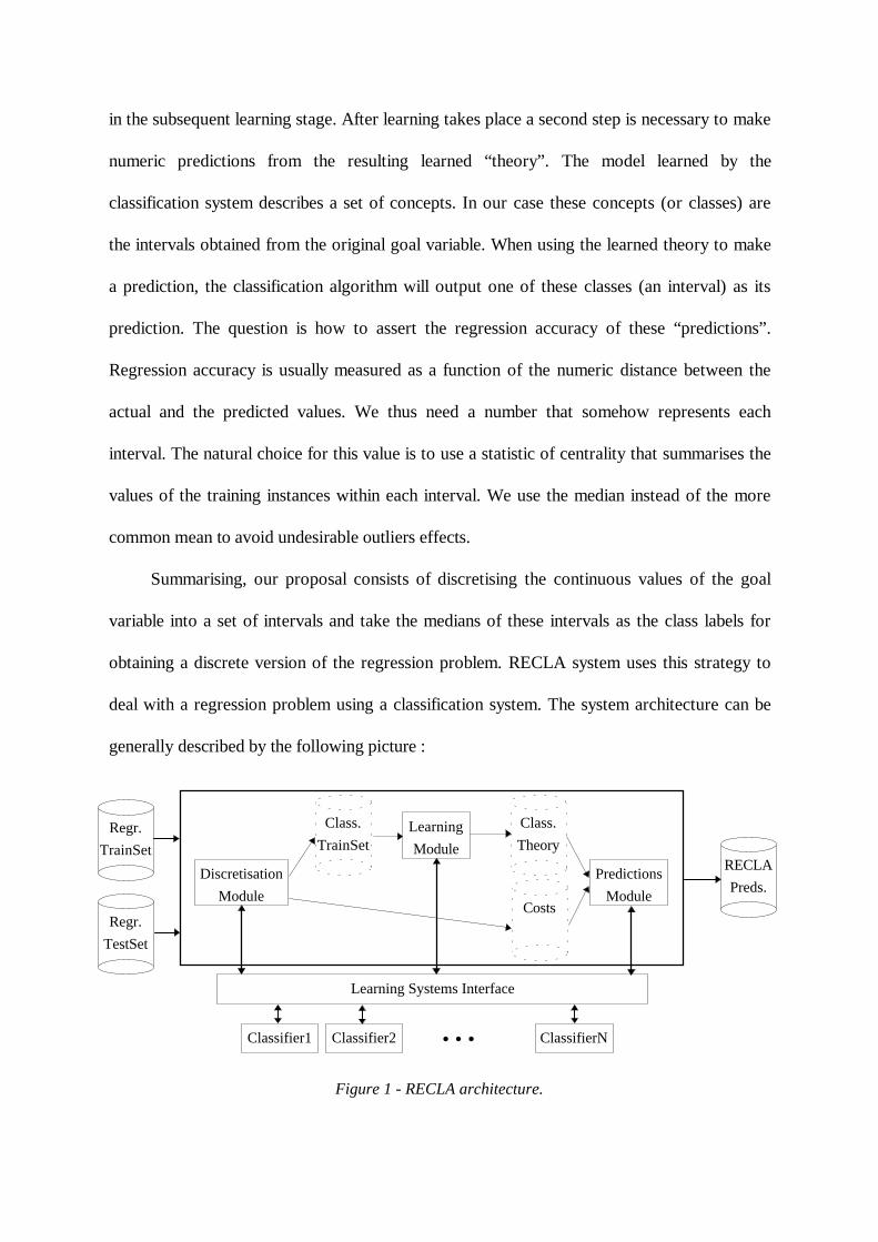
Summarising, our proposal consists of discretising the continuous values of the goal

variable into a set of intervals and take the medians of these intervals as the class labels for

obtaining a discrete version of the regression problem. RECLA system uses this strategy to

deal with a regression problem using a classification system. The system architecture can be

generally described by the following picture :

Figure 1 - RECLA architecture.

Learning

Module

Class.

TrainSet

Data

Costs

Class.

Theory

Discretisation

Module

Learning Systems Interface

Predictions

Module

Regr.

TrainSet

Data

Regr.

TestSet

Data

RECLA

Preds.

Classifier1 Classifier2 ClassifierN• • •

RECLA can be easily extended to other than the currently interfaced classification systems.

This may involve some coding effort in the learning systems interface module. This effort

should not be high as long as the target classification system works in a fairly standard way.

In effect, the only coding that it is usually necessary is related to different data set formats

used by RECLA and the target classification systems.

3 D i scr et i si ng a Cont i nuous Goal Var i ab l e

The main task that enables the use of classification algorithms in regression problems is the

transformation of a set of continuous values into a set of intervals. Two main questions arise

when performing this task. How many intervals to build and how to define the boundaries of

these intervals. The number of intervals will have a direct effect on both the accuracy and the

interpretabili ty of the resulting learned models. We argue that this decision is strongly

dependent on the target classification system. In effect, deciding how many intervals to build

is equivalent to deciding how many classes to use. This will change the class frequencies as

the number of training samples remains constant. Different class frequencies may affect

differently the classification algorithms due to the way they use the training data. This

motivated us to use a search-based approach to class discretisation.

3.1 Obtaining a Set of I ntervals

In this section we address the question of how to divide a set of continuous values into a set

of N intervals. We propose three alternative methods to achieve this goal :

• Equally probable intervals (EP) : This creates a set of N intervals with the same number

of elements. It can be said that this method has the focus on class frequencies and that it

makes the assumption that equal class frequencies is the best for a classification problem.

• Equal width intervals (EW) : The range of values is divided into N equal width intervals.

• K-means clustering (KM) : In this method the goal is to build N intervals that minimize the

sum of the distances of each element of an interval to its gravity center [4]. This method

starts with the EW approximation and then moves the elements of each interval to

contiguous intervals if these changes reduce the referred sum of distances. This is the more

sophisticated method and it seems to be the most coherent with the way we make

predictions with the learned model. In effect, as we use the median for making a

prediction, KM method seems to be minimizing the risk of making large errors.

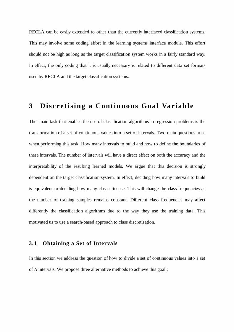
We present a simple example to better ill ustrate these methods. We use the Servo data set2

and we assume that the best number of intervals is 4. In the following figure we have divided

the original values into 20 equal width intervals to obtain a kind of histogram that somehow

captures the frequency distribution of the values.

No

of o

bs

0

10

20

30

40

50

60

70

80

0 0.5 1 1.5 2 2.5 3 3.5 4 4.5 5 5.5 6 6.5 7 7.5

Figure 2 - The distribution of the goal variable values in Servo.

2 In the appendix we provide details of the data sets used throughout the paper.

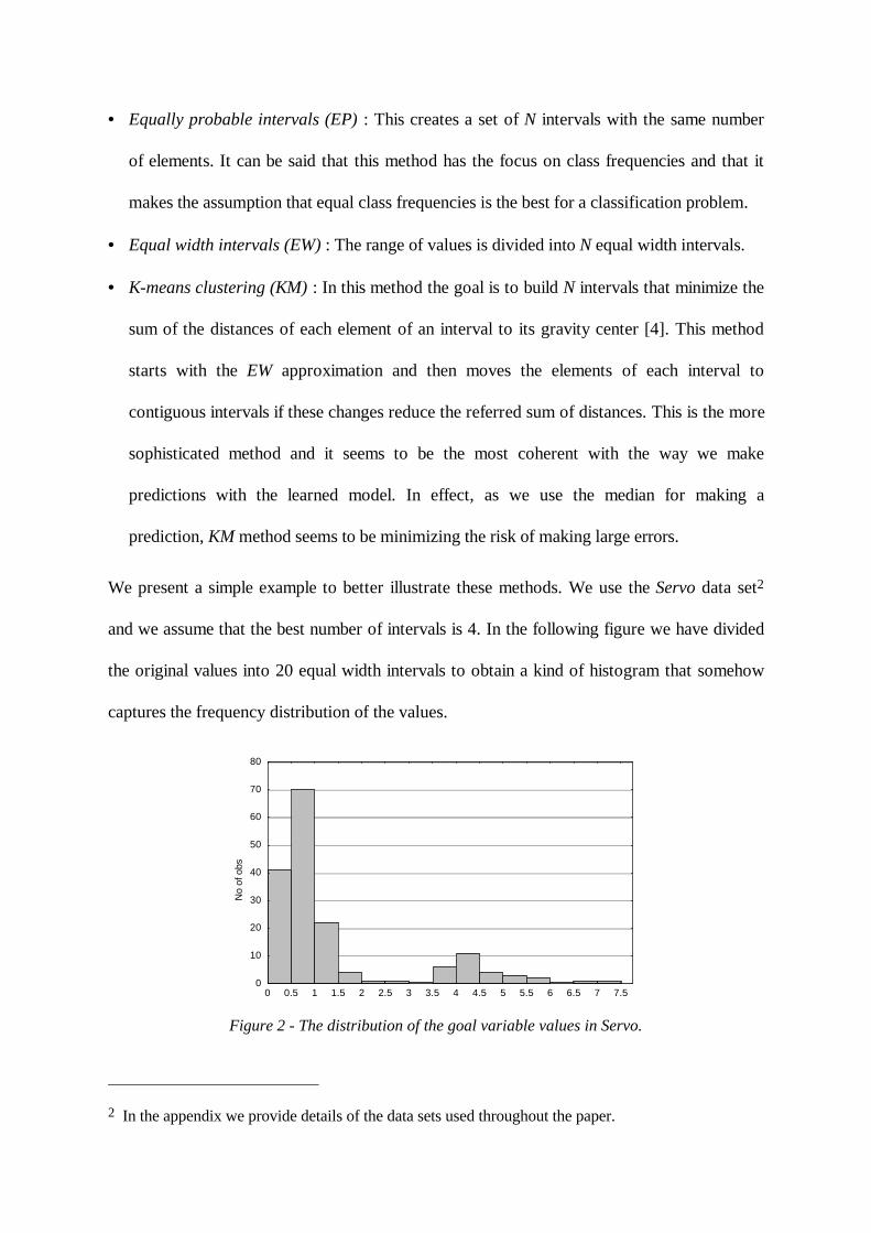
Using each of the three splitting strategies to obtain 4 intervals we get the following :

Table 1. Solutions found by the different methods.

Method Intervals Medians (class labels)KM ]0.13..0.45[ [0.45..0.79[ [0.79..3.20[ [3.20..7.10[ 0.34, 0.54, 1.03, 4.50EP ]0.13..0.50[ [0.50..0.75[ [0.75..1.30[ [1.30..7.10[ 0.36, .054, 0.94, 4.1EW ]0.13..1.87[ [1.87..3.62[ [3.62..5.36[ [5.36..7.10[ 0.56, 1.90, 4.40, 6.30

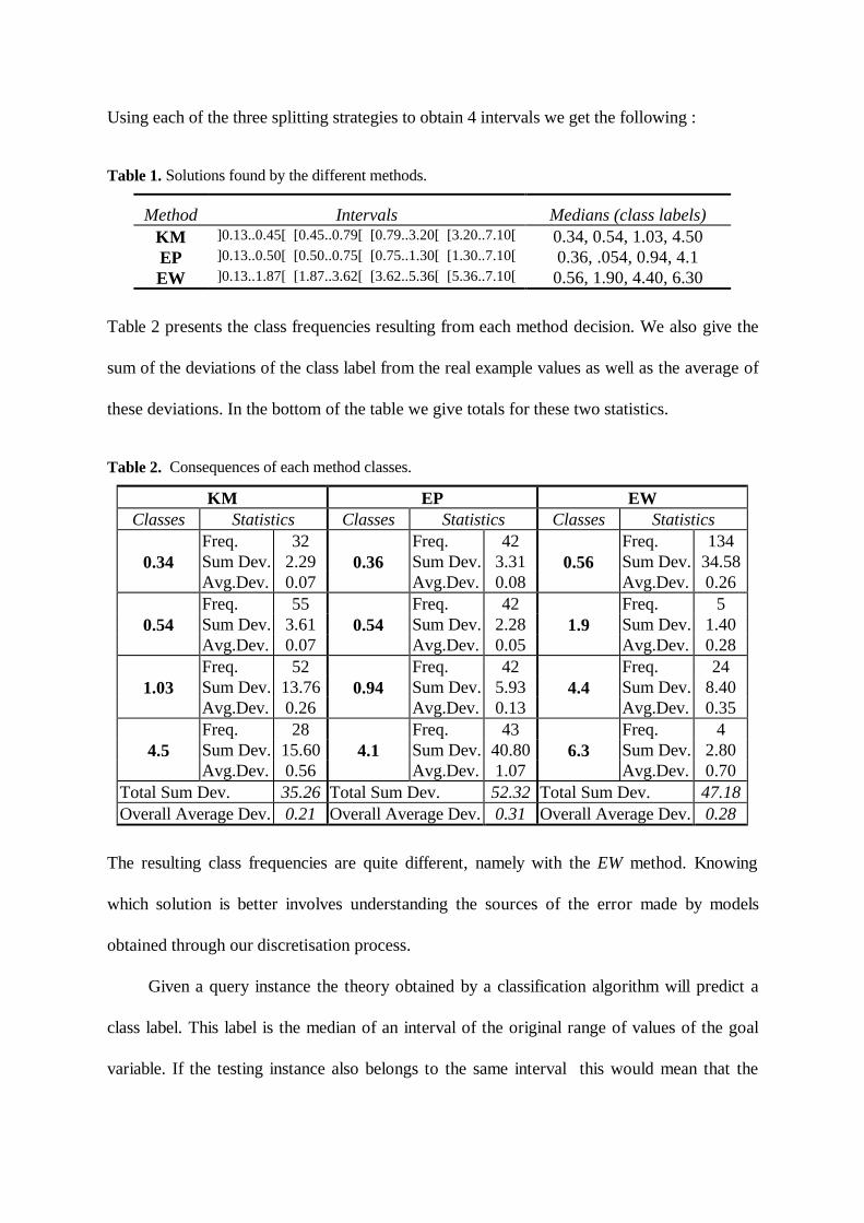
Table 2 presents the class frequencies resulting from each method decision. We also give the

sum of the deviations of the class label from the real example values as well as the average of

these deviations. In the bottom of the table we give totals for these two statistics.

Table 2. Consequences of each method classes.

KM EP EWClasses Statistics Classes Statistics Classes Statistics

Freq. 32 Freq. 42 Freq. 1340.34 Sum Dev. 2.29 0.36 Sum Dev. 3.31 0.56 Sum Dev. 34.58

Avg.Dev. 0.07 Avg.Dev. 0.08 Avg.Dev. 0.26Freq. 55 Freq. 42 Freq. 5

0.54 Sum Dev. 3.61 0.54 Sum Dev. 2.28 1.9 Sum Dev. 1.40Avg.Dev. 0.07 Avg.Dev. 0.05 Avg.Dev. 0.28Freq. 52 Freq. 42 Freq. 24

1.03 Sum Dev. 13.76 0.94 Sum Dev. 5.93 4.4 Sum Dev. 8.40Avg.Dev. 0.26 Avg.Dev. 0.13 Avg.Dev. 0.35Freq. 28 Freq. 43 Freq. 4

4.5 Sum Dev. 15.60 4.1 Sum Dev. 40.80 6.3 Sum Dev. 2.80Avg.Dev. 0.56 Avg.Dev. 1.07 Avg.Dev. 0.70

Total Sum Dev. 35.26 Total Sum Dev. 52.32 Total Sum Dev. 47.18Overall Average Dev.0.21 Overall Average Dev.0.31 Overall Average Dev.0.28

The resulting class frequencies are quite different, namely with the EW method. Knowing

which solution is better involves understanding the sources of the error made by models

obtained through our discretisation process.

Given a query instance the theory obtained by a classification algorithm will predict a

class label. This label is the median of an interval of the original range of values of the goal

variable. If the testing instance also belongs to the same interval this would mean that the

classification system predicted the correct class. However, this does not mean, that we have

the correct prediction in terms of regression. In effect, this predicted label can be “far” from

the true value being predicted. Thus high classification accuracy not necessarily corresponds

to high regression accuracy. The later is clearly damaged if few classes are used. However, if

more classes are introduced the class frequencies will start to decrease which will most

probably damage the classification accuracy. In order to observe the interaction between

these two types of errors when the number of classes is increased we have conducted a simple

experiment. Using a permutation of the Housing data set we have set the first 70% examples

as our training set and the remaining as testing set. Using C4.5 as learning engine we have

varied the number of classes from one to one hundred, collecting two types of error for each

trial. The first is the overall prediction error obtained by the resulting model on the testing set.

The second is the error rate of the same model (i.e. the percentage of classification errors

made by the model). For instance, if a testing instance has a Y value of 35 belonging to the

interval 25..40 with median 32, and C4.5 predicts class 57, we would count this as a

classification error (label 57 different from label 32), and would sum to the overall prediction

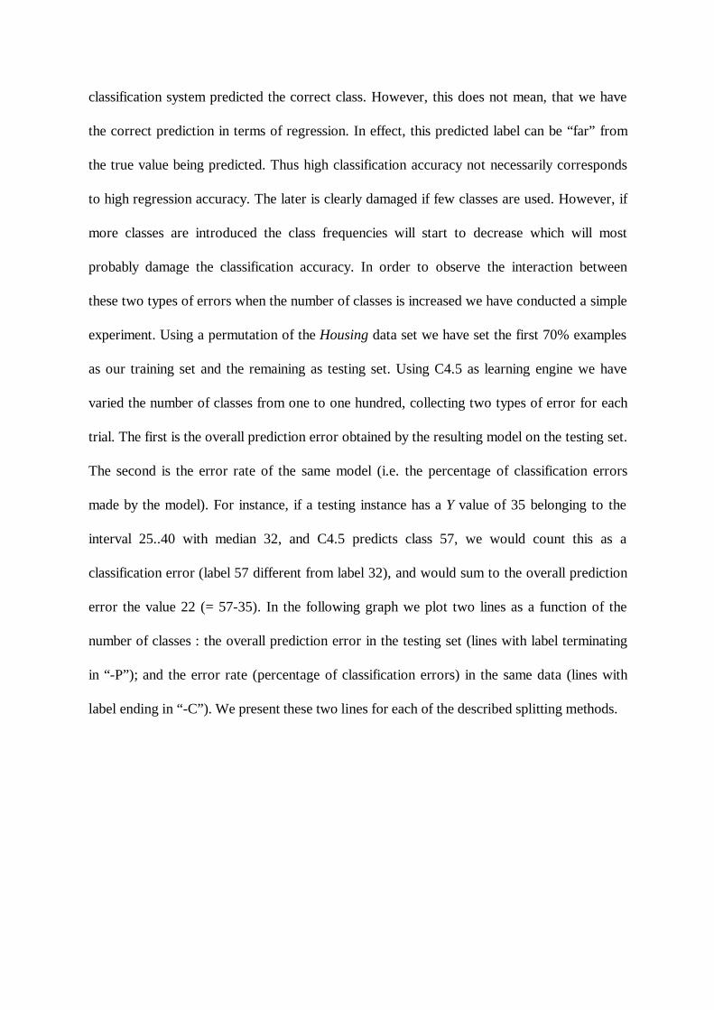
error the value 22 (= 57-35). In the following graph we plot two lines as a function of the

number of classes : the overall prediction error in the testing set (lines with label terminating

in “-P”); and the error rate (percentage of classification errors) in the same data (lines with

label ending in “-C”). We present these two lines for each of the described splitting methods.

0

1

2

3

4

5

6

7

1 5 9 13 17 21 25 29 33 37 41 45 49 53 57 61 65 69 73 77 81 85 89 93 97

Number of Classes

Ove

rall

Reg

ress

ion

Err

or

0%

10%

20%

30%

40%

50%

60%

70%

80%

90%

100%

Cla

ssifi

catio

n E

rror

KM-P EP-P EW-P KM-C EP-C EW-C

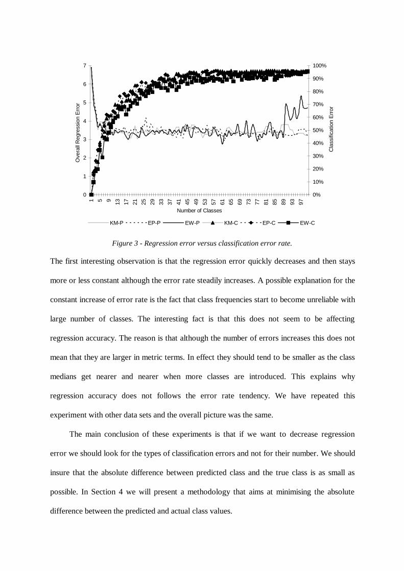
Figure 3 - Regression error versus classification error rate.

The first interesting observation is that the regression error quickly decreases and then stays

more or less constant although the error rate steadily increases. A possible explanation for the

constant increase of error rate is the fact that class frequencies start to become unreliable with

large number of classes. The interesting fact is that this does not seem to be affecting

regression accuracy. The reason is that although the number of errors increases this does not

mean that they are larger in metric terms. In effect they should tend to be smaller as the class

medians get nearer and nearer when more classes are introduced. This explains why

regression accuracy does not follows the error rate tendency. We have repeated this

experiment with other data sets and the overall picture was the same.

The main conclusion of these experiments is that if we want to decrease regression

error we should look for the types of classification errors and not for their number. We should

insure that the absolute difference between predicted class and the true class is as small as

possible. In Section 4 we will present a methodology that aims at minimising the absolute

difference between the predicted and actual class values.

Finally, an interesting conclusion to draw from Figure 3 is that in terms of

comprehensibili ty it is not worthwhile to try larger number of classes as the accuracy gains do

not compensate for complexity increase. In the following section we describe how RECLA

“walks” through the search space of “number of classes” and the guidance criteria it uses for

terminating the search for the “ideal” number of intervals.

3.2 Wr apping f or the Number of I ntervals

The splitting methods described in the previous section assumed that the number of intervals

was known. This section addresses the question of how to discover this number. We use a

wrapper [8, 9] approach as general search methodology. The number of intervals (i.e. the

number of classes) will have a direct effect on accuracy so it can be seen as a parameter of the

learning algorithm. Our goal is to set the value of this “parameter” such that the system

accuracy is optimised. As the number of ways of dividing a set of values into a set of intervals

is too large a heuristic search algorithm is necessary. The wrapper approach is a well known

strategy that has been mainly used for feature subset selection [8] and parameter estimation

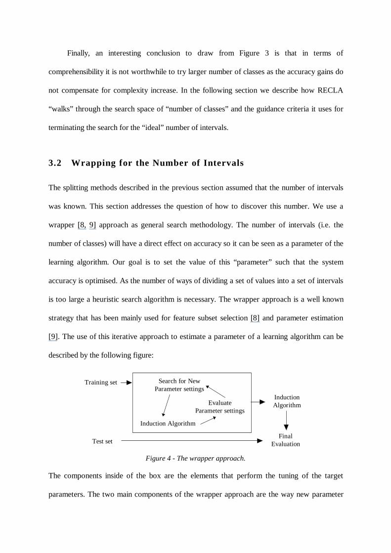
[9]. The use of this iterative approach to estimate a parameter of a learning algorithm can be

described by the following figure:

Training set

Test set

InductionAlgorithm

FinalEvaluation

Search for NewParameter settings

EvaluateParameter settings

Induction Algorithm

Figure 4 - The wrapper approach.

The components inside of the box are the elements that perform the tuning of the target

parameters. The two main components of the wrapper approach are the way new parameter

settings are generated and how their results are evaluated in the context of the target learning

algorithm. The basic idea is that of an iterative search procedure where different parameter

settings are tried and the setting that gives the best estimated accuracy is returned as the

result of the wrapper. This best setting will then be used by the learning algorithm in the real

evaluation using an independent test set. In our case this will correspond to getting the “best”

estimated number of intervals that will then be used to split the original continuous goal

values.

With respect to the search component we use a hill -climbing algorithm coupled with a

settable look-ahead parameter to minimise the well-known problem of local minima. Given a

tentative solution and the respective evaluation the search component is responsible for

generating a new trial. We provide the following two alternative search operators :

• Varying the number of intervals (VNI): This simple alternative consists of incrementing the

previously tried number of intervals by a constant value.

• Incrementally improving the number of intervals (INI) : The idea of this alternative is to

try to improve the previous set of intervals taking into account their individual evaluation.

For each trial we evaluate not only the overall result obtained by the algorithm but also the

error committed by each of the classes (intervals). The next set of intervals is built using

the median of these individual class error estimates. All intervals whose error is above the

median are further split. All the other intervals remain unchanged. This method provides a

kind of hierarchical interval structure for the goal variable which can also been considered

valuable knowledge in terms of understanding the problem being solved.

The search algorithm of the wrapper used by RECLA can be generally described by :

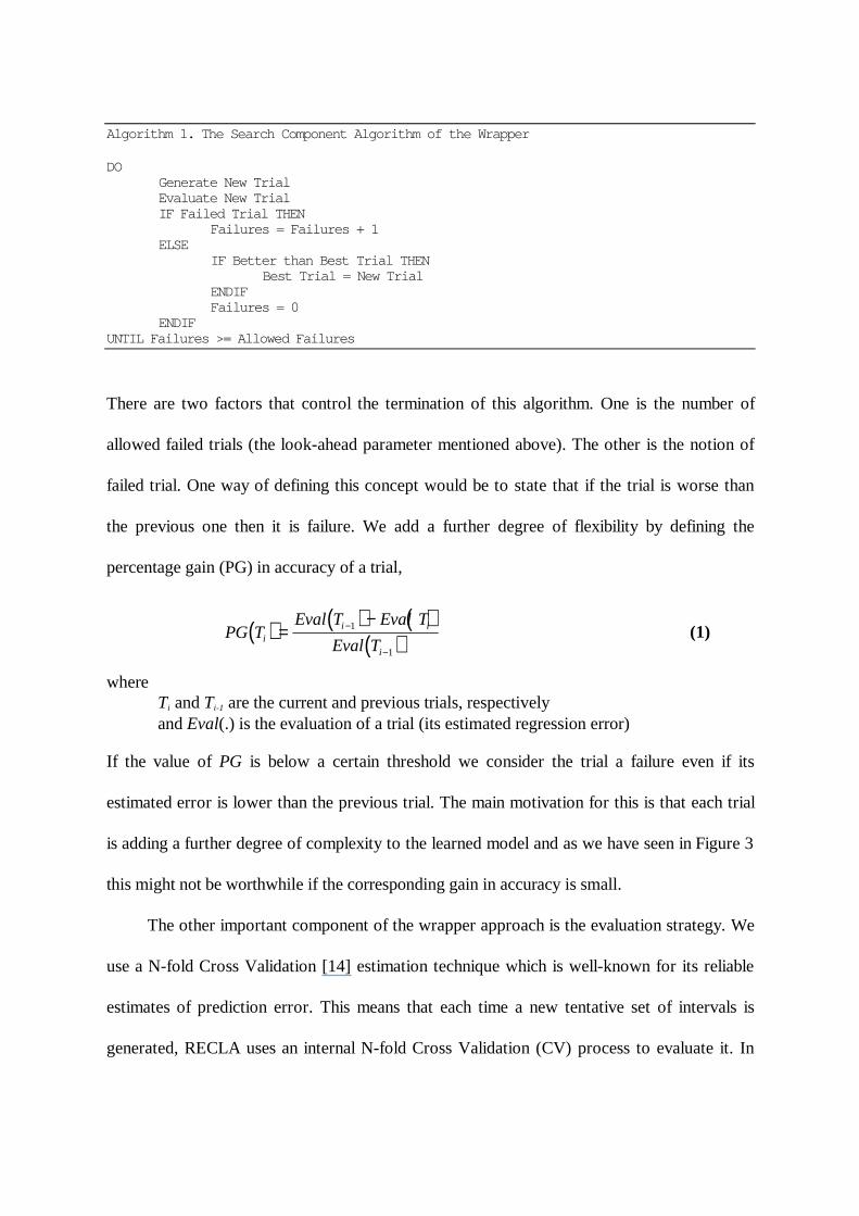
Algorithm 1. The Search Component Algorithm of the Wrapper

DOGenerate New TrialEvaluate New TrialIF Failed Trial THEN

Failures = Failures + 1ELSE

IF Better than Best Trial THENBest Trial = New Trial

ENDIFFailures = 0

ENDIFUNTIL Failures >= Allowed Failures

There are two factors that control the termination of this algorithm. One is the number of

allowed failed trials (the look-ahead parameter mentioned above). The other is the notion of

failed trial. One way of defining this concept would be to state that if the trial is worse than

the previous one then it is failure. We add a further degree of flexibili ty by defining the

percentage gain (PG) in accuracy of a trial,

( ) ( ) ( )( )PG T

Eval T Eval T

Eval Tii i

i

=−−

−

1

1

(1)

whereTi and Ti-1 are the current and previous trials, respectivelyand Eval(.) is the evaluation of a trial (its estimated regression error)

If the value of PG is below a certain threshold we consider the trial a failure even if its

estimated error is lower than the previous trial. The main motivation for this is that each trial

is adding a further degree of complexity to the learned model and as we have seen in Figure 3

this might not be worthwhile if the corresponding gain in accuracy is small.

The other important component of the wrapper approach is the evaluation strategy. We

use a N-fold Cross Validation [14] estimation technique which is well-known for its reliable

estimates of prediction error. This means that each time a new tentative set of intervals is

generated, RECLA uses an internal N-fold Cross Validation (CV) process to evaluate it. In

the next subsection we provide a small example of a discretisation process to better ill ustrate

our search-based approach.

3.2.1 An illustrative example

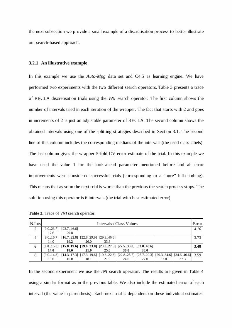
In this example we use the Auto-Mpg data set and C4.5 as learning engine. We have

performed two experiments with the two different search operators. Table 3 presents a trace

of RECLA discretisation trials using the VNI search operator. The first column shows the

number of intervals tried in each iteration of the wrapper. The fact that starts with 2 and goes

in increments of 2 is just an adjustable parameter of RECLA. The second column shows the

obtained intervals using one of the splitting strategies described in Section 3.1. The second

line of this column includes the corresponding medians of the intervals (the used class labels).

The last column gives the wrapper 5-fold CV error estimate of the trial. In this example we

have used the value 1 for the look-ahead parameter mentioned before and all error

improvements were considered successful trials (corresponding to a “pure” hill -climbing).

This means that as soon the next trial is worse than the previous the search process stops. The

solution using this operator is 6 intervals (the trial with best estimated error).

Table 3. Trace of VNI search operator.

N.Ints Intervals / Class Values Error2 [9.0..23.7]

17.6[23.7..46.6]

29.84.16

4 [9.0..16.7]14.0

[16.7..22.8]19.2

[22.8..29.9]26.0

[29.9..46.6]33.8

3.73

6 [9.0..15.8]14.0

[15.8..19.6]18.0

[19.6..23.0]21.0

[23.0..27.5]25.0

[27.5..33.0]30.0

[33.0..46.6]36.0

3.48

8 [9.0..14.3]13.0

[14.3..17.3]16.0

[17.3..19.6]18.1

[19.6..22.8]21.0

[22.8..25.7]24.0

[25.7..29.3]27.0

[29.3..34.6]32.0

[34.6..46.6]37.3

3.59

In the second experiment we use the INI search operator. The results are given in Table 4

using a similar format as in the previous table. We also include the estimated error of each

interval (the value in parenthesis). Each next trial is dependent on these individual estimates.

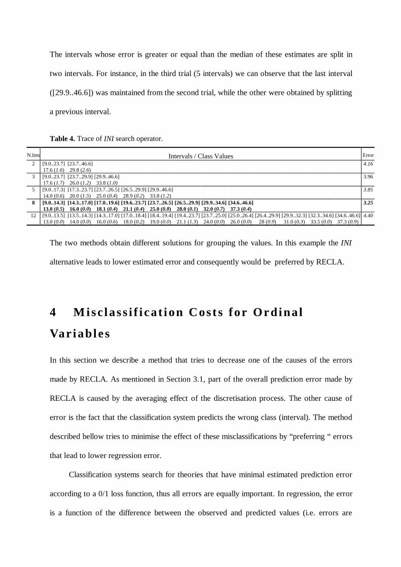
The intervals whose error is greater or equal than the median of these estimates are split in

two intervals. For instance, in the third trial (5 intervals) we can observe that the last interval

([29.9..46.6]) was maintained from the second trial, while the other were obtained by splitting

a previous interval.

Table 4. Trace of INI search operator.

N.Ints Intervals / Class Values Error

2 [9.0..23.7]17.6 (1.6)

[23.7..46.6]29.8 (2.6)

4.16

3 [9.0..23.7]17.6 (1.7)

[23.7..29.9]26.0 (1.2)

[29.9..46.6]33.8 (1.0)

3.96

5 [9.0..17.3]14.0 (0.6)

[17.3..23.7]20.0 (1.5)

[23.7..26.5]25.0 (0.4)

[26.5..29.9]28.9 (0.2)

[29.9..46.6]33.8 (1.2)

3.85

8 [9.0..14.3]13.0 (0.5)

[14.3..17.0]16.0 (0.0)

[17.0..19.6]18.1 (0.4)

[19.6..23.7]21.1 (0.4)

[23.7..26.5]25.0 (0.8)

[26.5..29.9]28.0 (0.1)

[29.9..34.6]32.0 (0.7)

[34.6..46.6]37.3 (0.4)

3.25

12 [9.0..13.5]13.0 (0.0)

[13.5..14.3]14.0 (0.0)

[14.3..17.0]16.0 (0.6)

[17.0..18.4]18.0 (0.2)

[18.4..19.4]19.0 (0.0)

[19.4..23.7]21.1 (1.3)

[23.7..25.0]24.0 (0.0)

[25.0..26.4]26.0 (0.0)

[26.4..29.9]28 (0.9)

[29.9..32.3]31.0 (0.3)

[32.3..34.6]33.5 (0.0)

[34.6..46.6]37.3 (0.9)

4.40

The two methods obtain different solutions for grouping the values. In this example the INI

alternative leads to lower estimated error and consequently would be preferred by RECLA.

4 M i scl assi f i cat i on Cost s f or Or d i nal

Var i ab l es

In this section we describe a method that tries to decrease one of the causes of the errors

made by RECLA. As mentioned in Section 3.1, part of the overall prediction error made by

RECLA is caused by the averaging effect of the discretisation process. The other cause of

error is the fact that the classification system predicts the wrong class (interval). The method

described bellow tries to minimise the effect of these misclassifications by “preferring “ errors

that lead to lower regression error.

Classification systems search for theories that have minimal estimated prediction error

according to a 0/1 loss function, thus all errors are equally important. In regression, the error

is a function of the difference between the observed and predicted values (i.e. errors are

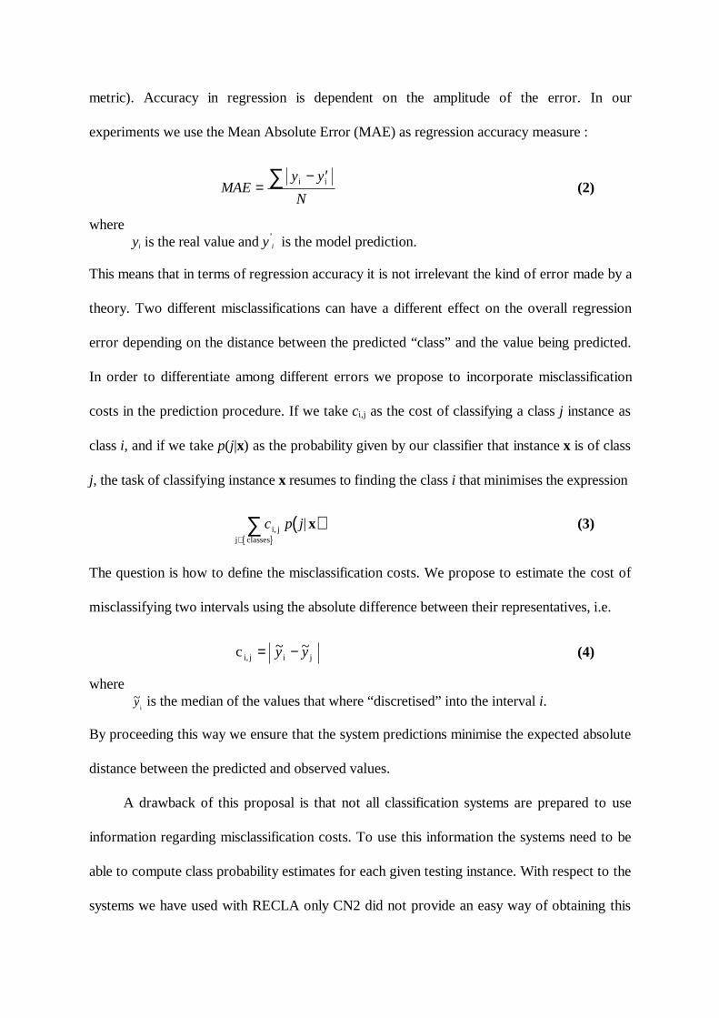
metric). Accuracy in regression is dependent on the amplitude of the error. In our

experiments we use the Mean Absolute Error (MAE) as regression accuracy measure :

MAEy y

N=

− ′∑ i i (2)

whereyi is the real value and y’

i is the model prediction.

This means that in terms of regression accuracy it is not irrelevant the kind of error made by a

theory. Two different misclassifications can have a different effect on the overall regression

error depending on the distance between the predicted “class” and the value being predicted.

In order to differentiate among different errors we propose to incorporate misclassification

costs in the prediction procedure. If we take ci,j as the cost of classifying a class j instance as

class i, and if we take p(j|x) as the probabili ty given by our classifier that instance x is of class

j, the task of classifying instance x resumes to finding the class i that minimises the expression

( ){ }

c p ji, jj classes

|x∈∑ (3)

The question is how to define the misclassification costs. We propose to estimate the cost of

misclassifying two intervals using the absolute difference between their representatives, i.e.

c i, j i j= −~ ~y y (4)

where~y

i is the median of the values that where “discretised” into the interval i.

By proceeding this way we ensure that the system predictions minimise the expected absolute

distance between the predicted and observed values.

A drawback of this proposal is that not all classification systems are prepared to use

information regarding misclassification costs. To use this information the systems need to be

able to compute class probabili ty estimates for each given testing instance. With respect to the

systems we have used with RECLA only CN2 did not provide an easy way of obtaining this

information. The used Linear Discriminant was prepared to work with misclassification costs

from scratch. With C4.5 it was necessary to make a program that used the class probabili ty

estimates of the trees learned by C4.5. This means that although the “standard” C4.5 is not

able to use misclassification costs, the version used within RECLA is able to use them.

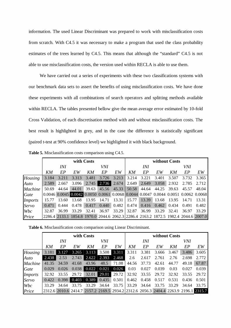
We have carried out a series of experiments with these two classifications systems with

our benchmark data sets to assert the benefits of using misclassification costs. We have done

these experiments with all combinations of search operators and splitting methods available

within RECLA. The tables presented bellow give the mean average error estimated by 10-fold

Cross Validation, of each discretisation method with and without misclassification costs. The

best result is highlighted in grey, and in the case the difference is statistically significant

(paired t-test at 90% confidence level) we highlighted it with black background.

Table 5. Misclassification costs comparison using C4.5.

with Costs without CostsINI VNI INI VNI

KM EP EW KM EP EW KM EP EW KM EP EWHousing 3.184 3.211 3.313 3.481 3.726 3.213 3.214 3.221 3.401 3.507 3.732 3.365Auto 2.589 2.667 3.096 2.745 2.736 2.674 2.649 2.649 3.058 2.932 2.785 2.712Machine 50.69 44.64 44.01 39.63 45.56 45.33 50.58 44.64 44.25 39.63 45.57 48.04Gate 0.0046 0.0045 0.0042 0.0050 0.0061 0.0068 0.0044 0.0047 0.0044 0.0051 0.0062 0.0068Imports 15.77 13.60 13.68 13.95 14.71 13.31 15.7713.39 13.68 13.95 14.71 13.31Servo 0.471 0.444 0.478 0.417 0.440 0.482 0.474 0.416 0.462 0.434 0.491 0.482Wbc 32.87 36.99 33.29 32.41 36.97 33.29 32.87 36.99 33.29 32.41 36.97 33.29Price 2286.4 2133.1 1854.8 1970.0 2044.6 2062.3 2286.4 2163.2 1872.5 1982.4 2044.62007.0

Table 6. Misclassification costs comparison using Linear Discriminant.

with Costs without CostsINI VNI INI VNI

KM EP EW KM EP EW KM EP EW KM EP EWHousing 3.181 3.127 3.265 3.113 3.508 3.311 3.311 3.381 3.666 3.4673.486 3.605Auto 2.438 2.53 2.743 2.622 2.393 2.468 2.6 2.617 2.761 2.76 2.698 2.772Machine 41.35 34.59 41.68 43.96 48.5 71.08 44.56 37.73 42.61 44.77 49.1867.87Gate 0.029 0.026 0.038 0.022 0.021 0.026 0.03 0.027 0.039 0.03 0.027 0.039Imports 32.92 33.55 29.72 32.01 29.01 29.72 32.92 33.55 29.72 32.92 33.55 29.72Servo 0.422 0.398 0.403 0.389 0.435 0.501 0.462 0.458 0.517 0.531 0.436 0.501Wbc 33.29 34.64 33.75 33.29 34.64 33.75 33.29 34.64 33.75 33.29 34.64 33.75Price 2312.6 2010.6 2414.7 2157.2 2169.5 2934.2 2312.6 2056.32404.4 2263.9 2196.12315.7

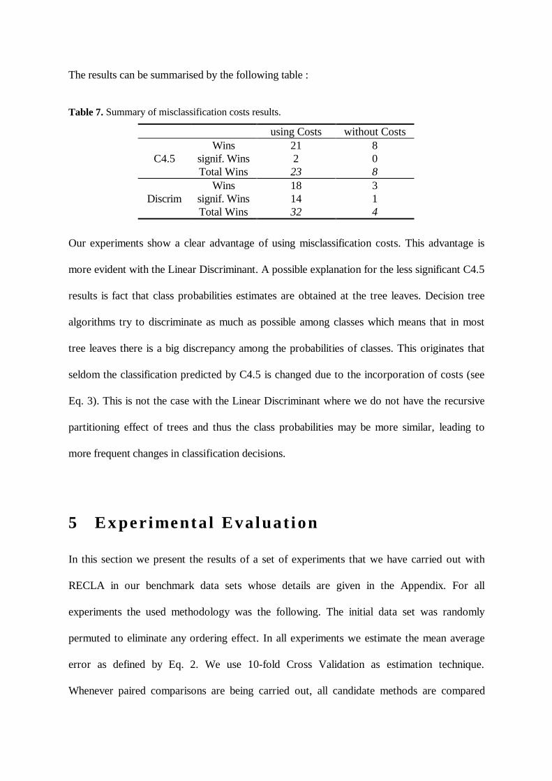
The results can be summarised by the following table :

Table 7. Summary of misclassification costs results.

using Costs without CostsWins 21 8

C4.5 signif. Wins 2 0Total Wins 23 8

Wins 18 3Discrim signif. Wins 14 1

Total Wins 32 4

Our experiments show a clear advantage of using misclassification costs. This advantage is

more evident with the Linear Discriminant. A possible explanation for the less significant C4.5

results is fact that class probabili ties estimates are obtained at the tree leaves. Decision tree

algorithms try to discriminate as much as possible among classes which means that in most

tree leaves there is a big discrepancy among the probabili ties of classes. This originates that

seldom the classification predicted by C4.5 is changed due to the incorporation of costs (see

Eq. 3). This is not the case with the Linear Discriminant where we do not have the recursive

partitioning effect of trees and thus the class probabili ties may be more similar, leading to

more frequent changes in classification decisions.

5 Ex per i ment al Eval uat i on

In this section we present the results of a set of experiments that we have carried out with

RECLA in our benchmark data sets whose details are given in the Appendix. For all

experiments the used methodology was the following. The initial data set was randomly

permuted to eliminate any ordering effect. In all experiments we estimate the mean average

error as defined by Eq. 2. We use 10-fold Cross Validation as estimation technique.

Whenever paired comparisons are being carried out, all candidate methods are compared

using the same 10 train/test folds. We use paired t-Student tests for asserting the significance

of observed differences.

5.1 Evaluat ion of the Discret i sat ion M ethods

The method used by RECLA to discretise the goal variable of a regression problem depends

on two main issues as we have seen in Section 3 : the splitting method and the search

operator used for generating new trials. This leads to 6 different discretisation methods.

RECLA can use a specific method or try all and chose the one that gives better estimated

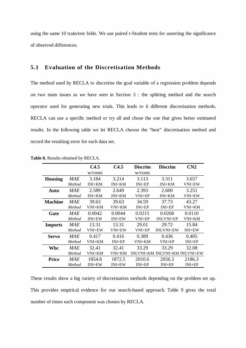
results. In the following table we let RECLA choose the “best” discretisation method and

record the resulting error for each data set.

Table 8. Results obtained by RECLA.

C4.5w/costs

C4.5 Discrimw/costs

Discrim CN2

Housing MAE 3.184 3.214 3.113 3.311 3.657Method INI+KM INI+KM INI+EP INI+KM VNI+EW

Auto MAE 2.589 2.649 2.393 2.600 3.251Method INI+KM INI+KM VNI+EP INI+KM VNI+EW

Machine MAE 39.63 39.63 34.59 37.73 43.27Method VNI+KM VNI+KM INI+EP INI+EP VNI+KM

Gate MAE 0.0042 0.0044 0.0215 0.0268 0.0110Method INI+EW INI+EW VNI+EP INI;VNI+EP VNI+KM

Imports MAE 13.31 13.31 29.01 29.72 15.84Method VNI+EW VNI+EW VNI+EP INI;VNI+EW INI+EW

Servo MAE 0.417 0.416 0.389 0.436 0.405Method VNI+KM INI+EP VNI+KM VNI+EP INI+EP

Wbc MAE 32.41 32.41 33.29 33.29 32.08Method VNI+KM VNI+KM INI;VNI+KM INI;VNI+KM INI;VNI+EW

Price MAE 1854.8 1872.5 2010.6 2056.3 2186.3Method INI+EW INI+EW INI+EP INI+EP INI+EP

These results show a big variety of discretisation methods depending on the problem set up.

This provides empirical evidence for our search-based approach. Table 9 gives the total

number of times each component was chosen by RECLA.

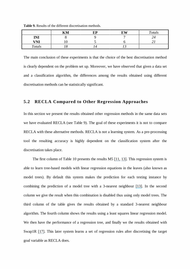
Table 9. Results of the different discretisation methods.

KM EP EW TotalsINI 8 9 7 24VNI 10 5 6 21

Totals 18 14 13

The main conclusion of these experiments is that the choice of the best discretisation method

is clearly dependent on the problem set up. Moreover, we have observed that given a data set

and a classification algorithm, the differences among the results obtained using different

discretisation methods can be statistically significant.

5.2 RECL A Compared to Other Regression Appr oaches

In this section we present the results obtained other regression methods in the same data sets

we have evaluated RECLA (see Table 9). The goal of these experiments it is not to compare

RECLA with these alternative methods. RECLA is not a learning system. As a pre-processing

tool the resulting accuracy is highly dependent on the classification system after the

discretisation takes place.

The first column of Table 10 presents the results M5 [11, 13]. This regression system is

able to learn tree-based models with linear regression equations in the leaves (also known as

model trees). By default this system makes the prediction for each testing instance by

combining the prediction of a model tree with a 3-nearest neighbour [13]. In the second

column we give the result when this combination is disabled thus using only model trees. The

third column of the table gives the results obtained by a standard 3-nearest neighbour

algorithm. The fourth column shows the results using a least squares linear regression model.

We then have the performance of a regression tree, and finally we the results obtained with

Swap1R [17]. This later system learns a set of regression rules after discretising the target

goal variable as RECLA does.

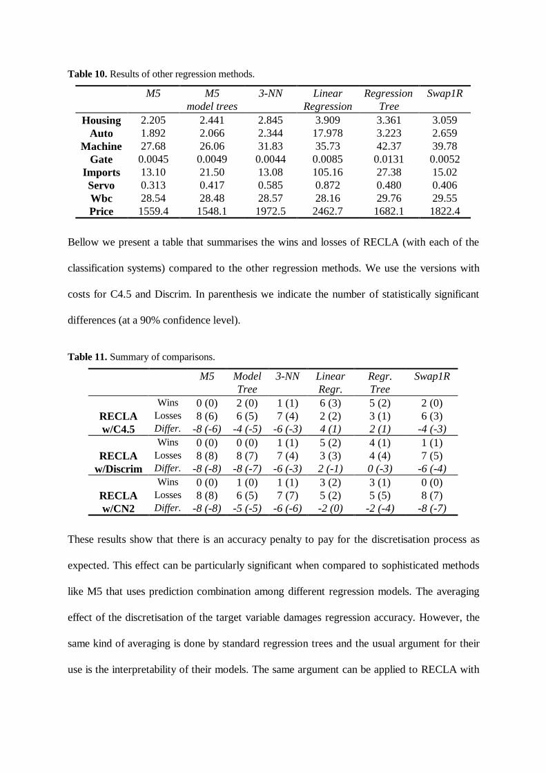
Table 10. Results of other regression methods.

M5 M5model trees

3-NN LinearRegression

RegressionTree

Swap1R

Housing 2.205 2.441 2.845 3.909 3.361 3.059Auto 1.892 2.066 2.344 17.978 3.223 2.659

Machine 27.68 26.06 31.83 35.73 42.37 39.78Gate 0.0045 0.0049 0.0044 0.0085 0.0131 0.0052

Imports 13.10 21.50 13.08 105.16 27.38 15.02Servo 0.313 0.417 0.585 0.872 0.480 0.406Wbc 28.54 28.48 28.57 28.16 29.76 29.55Price 1559.4 1548.1 1972.5 2462.7 1682.1 1822.4

Bellow we present a table that summarises the wins and losses of RECLA (with each of the

classification systems) compared to the other regression methods. We use the versions with

costs for C4.5 and Discrim. In parenthesis we indicate the number of statistically significant

differences (at a 90% confidence level).

Table 11. Summary of comparisons.

M5 ModelTree

3-NN LinearRegr.

Regr.Tree

Swap1R

Wins 0 (0) 2 (0) 1 (1) 6 (3) 5 (2) 2 (0)RECLA Losses 8 (6) 6 (5) 7 (4) 2 (2) 3 (1) 6 (3)w/C4.5 Differ. -8 (-6) -4 (-5) -6 (-3) 4 (1) 2 (1) -4 (-3)

Wins 0 (0) 0 (0) 1 (1) 5 (2) 4 (1) 1 (1)RECLA Losses 8 (8) 8 (7) 7 (4) 3 (3) 4 (4) 7 (5)

w/Discrim Differ. -8 (-8) -8 (-7) -6 (-3) 2 (-1) 0 (-3) -6 (-4)Wins 0 (0) 1 (0) 1 (1) 3 (2) 3 (1) 0 (0)

RECLA Losses 8 (8) 6 (5) 7 (7) 5 (2) 5 (5) 8 (7)w/CN2 Differ. -8 (-8) -5 (-5) -6 (-6) -2 (0) -2 (-4) -8 (-7)

These results show that there is an accuracy penalty to pay for the discretisation process as

expected. This effect can be particularly significant when compared to sophisticated methods

like M5 that uses prediction combination among different regression models. The averaging

effect of the discretisation of the target variable damages regression accuracy. However, the

same kind of averaging is done by standard regression trees and the usual argument for their

use is the interpretabili ty of their models. The same argument can be applied to RECLA with

either C4.5 or CN2. It is interesting to notice that RECLA with C4.5 is quite competitive

with the regression tree.

It is clear from the experiments we have carried out that the used learning engine can

originate significant differences in terms of regression accuracy. This can be confirmed when

looking at Swap1R results. This system deals with regression using the same process of

transforming it into a classification problem. It uses an algorithm called P-class that splits the

continuous values into a set of K intervals. This algorithm is basically the same as K-means

(KM). Swap1R asks for the number of classes (intervals) to use3, although the authors

suggest that this number could be found by cross validation [17]. As the discretisation method

is equal to one of the methods provided by RECLA, the better results of Swap1R can only be

caused by its classification learning algorithm. This means that the results obtained by

RECLA could also be better if other learning engines were tried.

6 Rel at ed Wor k

Mapping regression into classification was first proposed in Weiss and Indurkhya’s work [16,

17]. These authors incorporate the mapping within their regression system. They use an

algorithm called P-class which is basically the same as ours KM method. Compared to this

work we added other alternative discretisation methods and empirically proved the

advantages of a search-based approach to class discretisation. Moreover, by separating the

discretisation process from the learning algorithm we extended this approach to other

systems. Finally, we have introduced the use of misclassification costs to overcome the

3 In these experiments we have always used 5 classes following a suggestion of one of the authors ofSwap1R (Nitin Indurkhya).

inadequacy of classification systems to deal with ordinal target variables. This originated a

significant gain in regression accuracy as our experiments have shown.

The vast research are on continuous attribute discretisation usually proceeds by trying

to maximise the mutual information between the resulting discrete attribute and the classes

[5]. This strategy is applicable only when the classes are given. Ours is a different problem, as

we are determining which classes to consider.

7 Concl usi ons

The method described in this paper enables the use of classification systems on regression

tasks. The significance of this work is two-fold. First, we have managed to extend the

applicabili ty of a wide range of ML systems. Second, our methodology provides an

alternative trade-off between regression accuracy and comprehensibili ty of the learned

models. Our method also provides a better insight about the structure of the target variable by

dividing its values into significant intervals, which extends our understanding of the domain.

We have presented a set of alternative discretisation methods and demonstrated their

validity through experimental evaluation. Moreover, we have added misclassifications costs

which provide a better theoretical justification for using classification systems on regression

tasks. We have used a search-based approach which is justified by our experimental results

which show that the best discretisation is often dependent on both the domain and the

induction tool.

Our proposals were implemented in a system called RECLA which we have applied in

conjunction with three different classification systems. These systems are quite different from

each other which again provides evidence for the high generality of our methods. The system

is easily extendible to other classification algorithms thus being a useful tool for the users of

existing classification systems.

Finally, we have compared the results obtained by RECLA using the three learning

engines, to other standard regression methods. The results of these comparisons show that

although RECLA can be competitive with some algorithms, still i t is has lower accuracy than

some state-of-the-art regression systems. These results are obviously dependent on the

learning engine used as our experiments have shown. Comparison with Swap1R, that uses a

similar mapping strategy, reveal that better regression accuracy is achievable if other learning

engines are used.

A ck now l edgemen t s

Thanks are due to the authors of the classification systems we have used in our experimentsfor providing them to us.

Ref e rences

1. Breiman,L. , Friedman,J.H., Olshen,R.A. and Stone,C.J., Classifi cation and Regression Trees,Wadsworth Int. Group, Belmont, California, USA, 1984.

2. Bhattacharyya,G. and Johnson,R., Statistical Concepts and Methods. John Wiley & Sons, 1977.

3. Clark, P. and Niblett, T., The CN2 induction algorithm, Machine Learning, 3(4), 261-283, 1989.

4. Dillon,W. and Goldstein,M., Multivariate Analysis. John Wiley & Sons, Inc, 1984

5. Fayyad, U.M., and Irani, K.B. , Multi-interval Discretization of Continuous-valued Attributes forClassification Learning, in Proceedings of the 13th International Joint Conference on Artifi cialIntelligence (IJCAI-93). Morgan Kaufmann Publishers, 1993.

6. Fisher, R.A., The use of multiple measurements in taxonomic problems, Annals of Eugenics. 7,179-188, 1936.

7. Fix, E. and Hodges, J.L., Discriminatory analysis, nonparametric discrimination consistencyproperties, Technical Report 4, Randolph Field, TX: US Air Force, School of Aviation Medicine,1951.

8. John,G.H., Kohavi,R. and Pfleger, K., Irrelevant features and the subset selection problem., inProceedings of the 11th IML, Morgan Kaufmann, 1994.

9. Kohavi, R., Wrappers for performance enhancement and oblivious decision graphs, PhD Thesis,1995.

10. Merz,C.J. and Murphy,P.M., UCI repository of machine learning databases[http://www.ics.uci.edu/MLRepository.html]. Irvine, CA. University of Cali fornia, Department ofInformation and Computer Science, 1996.

11. Quinlan, J.R., Learning with Continuos Classes, in Proceedings of the 5th Australian JointConference on Artificial Intelligence. Singapore: World Scientific, 1992.

12. Quinlan, J. R., C4.5 : programs for machine learning. Morgan Kaufmann Publishers ,1993.

13. Quinlan,J.R., Combining Instance-based and Model-based Learning, in Proceedings of the 10thICML, Morgan Kaufmann, 1993.

14. Stone, M. , Cross-validatory choice and assessment of statistical predictions, Journal of the RoyalStatistical Society. B 36, 111-147, 1974.

15. Torgo,L. Gama,J., Search-based Class Discretisation, in Proceedings of the EuropeanConference on Machine Learning (ECML-97), van Someren,M, and Widmer,G, (eds.), Lecture Notesin Artificial Intelligence, 1224, 266-273, Springer-Verlag, 1997.

16. Weiss, S. and Indurkhya, N., Rule-base Regression, in Proceedings of the 13th InternationalJoint Conference on Artificial Intelligence. 1072-1078, 1993.

17. Weiss, S. and Indurkhya, N., Rule-based Machine Learning Methods for Functional Prediction, inJournal Of Artificial Intelligence Research (JAIR). 3, 383-403, 1995.

A ppend i x

Most of the data sets we have used were obtained from the UCI Machine LearningRepository [http://www.ics.uci.edu/MLRepository.html]. The main characteristics of the useddomains as well as eventual modifications made to the original databases are describedbellow:

• Housing - this data set contains 506 instances described by 13 continuous input variables.The goal consists of predicting the housing values in suburbs of Boston.

• Auto (Auto-Mpg database) - 398 instances described by 3 nominal and 4 continuousvariables. The target variable is the fuel consumption (miles per gallon).

• Servo - 167 instances; 4 nominal attributes.• Machine (Computer Hardware database) - 209 instances; 6 continuous attributes. The

goal is to predict the cpu relative performance based on other computer characteristics.• Price (Automobile database) - 159 cases; 16 continuous attributes. This data set is built

from the Automobile database by removing all instances with unknown values from theoriginal 205 cases. Nominal attributes were also removed. The goal is to predict the carprices based on other characteristics.

• Imports (Automobile database) - based on the same database we have built a different dataset consisting of 164 instances described by 11 nominal attributes and 14 continuousvariables. From the original data we only removed the cases with unknown value on theattribute “normalized-losses” . This attribute describes the car insurance normalized losses.This variable was taken as the predicting goal.

• Wbc (Wisconsin Breast Cancer databases) - predicting recurrence time in 194 breastcancer cases (4 instances with unknowns removed); 32 continuous attributes.

• Gate (non-UCI data set) - 300 instances; 10 continuous variables. The problem consists ofpredicting the time to collapse of an electrical network based on some monitoring variablevalues.