Embed Size (px)
Citation preview
Reliability assessment of shallow foundations on undrained soilsconsidering soil spatial variability
J.T. Simõesa, Luis C. Nevesb, Armando N. Antãoa,∗, Nuno M. C. Guerraa
aUNIC, Department of Civil Engineering, Faculdade de Ciências e Tecnologia, Universidade Nova deLisboa, Portugal
bResilience Engineering Research Group, Faculty of Engineering, University of Nottingham, UK
Abstract
Structural design using partial safety factors aims at achieving an homogeneous safetylevel in geotechnical design without the use of more complex reliability analysis. In thiswork, the different Design Approaches proposed by Eurocode 7 for shallow foundationsresting on the surface of undrained soils are compared in terms of the resulting reliabilityindices. The influence of both centered and eccentric loads, as well as homogeneous andheterogeneous isotropic and anisotropic distributions for the variability of soil propertieswere investigated in the reliability analysis.
A finite element implementation of the upper bound theorem of limit analysis is com-bined with Latin Hypercube sampling to compute the probabilistic response of shallowfoundations. Considering realistic probabilistic distributions for both permanent and liveloads, First Order Reliability Method is used to calculate the reliability index of suchstructures designed according to the different Design Approaches present in Eurocode 7.
The results obtained show that the Eurocode 7 leads to satisfactory reliability indices,but that significant differences between Design Approaches exist.
Keywords: Reliability assessment, Eurocode 7, anisotropic soil spatial variability,upper bound theorem, bearing capacity, uncertainty of load eccentricity
1. Introduction1
The partial safety factors method is a semi-probabilistic safety verification method2
aiming at attaining uniform and consistent safety levels, without the complexity of ex-3
plicit reliability analysis. That approach is employed in Eurocode 7 [11] for geotechnical4
limit states through the use of three different Design Approaches. These approaches5
should result in uniform safety levels, consistent with the target reliability indices pre-6
scribed in Eurocode 0 [10]. However, the different Design Approaches proposed in Eu-7
rocode 7 [11] can, potentially, result in structures with very different levels of safety, and8
∗Corresponding authorEmail addresses: [email protected] (J.T. Simões), [email protected] (Luis C.
Neves), [email protected] (Armando N. Antão), [email protected] (Nuno M. C. Guerra)
Preprint submitted to Elsevier November 27, 2019
a reliability analysis can assess the consistency of the methods proposed in codes [32,9
e.g.].10
In the partial safety factors method, the large uncertainties present in geotechnical11
design [38, 39, 53, e.g.] are considered through the use of nominal values of properties12
and safety factors applied to loads, soil properties and resistances [11].13
The present paper aims at evaluating the reliability of the bearing capacity of shallow14
foundations under undrained conditions. For such analysis, it is paramount to consider15
explicitly the uncertainty and heterogeneity characteristics of soils. According to Phoon16
and Kulhawy [38], uncertainties in soil properties result from (i) inherent variability, (ii)17
errors in the performed measurements and (iii) errors from transformation of experimen-18
tal tests results to mechanical properties. It has been shown that uncertainties like the19
inherent variability can significantly influence the failure mode and the bearing capacity20
of shallow foundations [22, 23, 19, see e.g.]. Moreover, the uncertainty in loading must21
also be considered, in particular in what regards the eccentricity of applied loads. In22
fact, due to uncertainty in the amplitude of different loads, random deviations in the23
point of application of the resulting load may arise, influencing the failure mode of the24
foundation and its safety.25
The collapse load of foundations under these conditions can be computed using dif-26
ferent numerical approaches. In this paper, bearing capacity is determined using a finite27
element implementation of the limit analysis upper bound theorem, the Sublim3D code,28
described in [45]. The ability of the mentioned implementation to compute upper bound29
solutions of various problems has been previously demonstrated [44, 43, 4]. This code30
uses a parallel algorithm which significantly reduces the computational time. Calcula-31
tions were performed in a cluster with 104 cores.32
The use of advanced numerical methods for computing the collapse load of foundations33
limits the use of gradient-based reliability methods (e.g.,, FORM – First Order Reliability34
Method – and SORM – Second Order Reliability Method), making simulation the most35
effective tool for reliability assessment. To assess the methodology proposed in Eurocode36
7 [11], the reliability index of a set of shallow foundations designed according to its three37
Design Approaches (DA) is evaluated. The foundations under analysis are continuous38
footings on soil responding in undrained conditions. For these, two-dimensional models39
are usually employed and, due to their lower computational cost, will also be used here.40
The spatial variability of the soil properties, and therefore its heterogeneity, can be41
considered using random fields [38, e.g.]. Random fields can be generated using a wide42
range of approaches [15, 20, 16]. To reduce the number of samples required for achieving43
acceptable results, Latin Hypercube sampling was employed in this work [34, 21, 36]. This44
method was also used by Cho and Park [13] to study the same geotechnical problem.45
Based on the available information on the probabilistic properties of soil [33, 51, 5, 31,46
24, 47, 12, 40, 42, 38, 39, 14, 6, e.g.], a parametric study varying these properties is47
presented.48
The influence of the soil spatial variability on various geotechnical problems has al-49
ready been investigated [19]. With respect specifically to shallow foundations, servicia-50
bility limit states have been considered for different cases: plane strain single footing51
[37, 19, 1], plane strain double footings [17, 2] and 3D single and double footings [18, 19];52
these contributions used vertical loading, but inclined loads were also considered [3].53
Moreover, the ultimate limit state problem has been deeply studied in the last years.54
The ultimate limit state of shallow foundations resting on soils responding in undrained55
2
conditions have already been greatly investigated [22, 23, 41, 13, 28, 9, 27] consider-56
ing different probabilistic distributions for the undrained shear strength, adopting both57
isotropic and anisotropic structures for the spatial correlations and using different meth-58
ods to generate the random fields. Most of the works investigated only the case of a59
vertical centered load [22, 23, 41, 13, 28, 27] and only a recent work [9] considered the60
effect of combination of horizontal and vertical loads, together with moments. In gen-61
eral, these works combined the use of conventional non-linear finite elements analyses or62
numerical limit analyses with random field theory and Monte Carlo simulations.63
The previously mentioned works have clearly shown that average bearing capacity64
considering the soil spatial variability is smaller than the one calculating admitting an65
homogeneous soil. However, the impact of spatial variability of soil on the safety of foun-66
dations considering the different Design Approaches proposed in Eurocode 7 in unknown.67
Do the Design Approaches of Eurocode 7 meet the desired level of safety for a wide range68
of foundations when the spatial variability is considered?69
In the present paper, reliability analysis is used to assess the level of safety of shal-70
low foundations under undrained conditions of the Design Approaches of Eurocode 771
considering soil heterogeneity and the uncertainty of the eccentricity of the load. The72
soil heterogeneity is defined by the statistical properties of the undrained shear strength,73
cu: mean, coefficient of variation and anisotropic correlation length. The uncertainty of74
the load is considered through a statistical distribution of its eccentricity. The obtained75
results are fitted to a range of probabilistic distributions for each set of parameters char-76
acterizing the soil. These are then used to compute the reliability index using the First77
Order Reliability Method (FORM) [48, 29] for foundations designed following Eurocode78
7 [11].79
2. Problem definition80
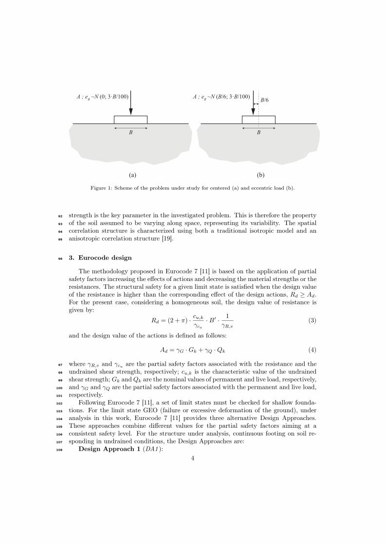
The problem studied is a strip shallow foundation with width B on the surface of81
undrained soil, submitted to two load cases (centered and eccentric load), as presented82
in Figure 1. The eccentricity, eB , of the vertical load is assumed to be described by a83
normal distribution, being for each load case defined as:84
Load case 1: eB ∼N(0; 3B/100)85
Load case 2: eB ∼N(B/6; 3B/100)86
The mean eccentricity considered in Load case 2 corresponds to the maximum value87
for which, in the homogeneous case, the base of the footing remains under compression.88
Therefore, the conclusions of the study are limited to these cases.89
The bearing capacity of the foundation considering a two-dimensional plane strainproblem and a homogeneous soil can be determined by:
R = Nc · cu ·B′ (1)
where Nc is a bearing capacity factor, equal to 2 + π, cu is the undrained shear strengthand B′ is the effective width, defined as:
B′ = B − 2 · eB (2)
For heterogeneous soils, no closed form expression for the bearing capacity can be defined,90
and numerical methods must be used. As shown in Equation 1, the undrained shear91
3
B B
B/6A ; e
B ~N (0; 3·B/100) A ; e
B ~N (B/6; 3·B/100)
(b)(a)
Figure 1: Scheme of the problem under study for centered (a) and eccentric load (b).
strength is the key parameter in the investigated problem. This is therefore the property92
of the soil assumed to be varying along space, representing its variability. The spatial93
correlation structure is characterized using both a traditional isotropic model and an94
anisotropic correlation structure [19].95
3. Eurocode design96
The methodology proposed in Eurocode 7 [11] is based on the application of partialsafety factors increasing the effects of actions and decreasing the material strengths or theresistances. The structural safety for a given limit state is satisfied when the design valueof the resistance is higher than the corresponding effect of the design actions, Rd ≥ Ad.For the present case, considering a homogeneous soil, the design value of resistance isgiven by:
Rd = (2 + π) · cu,kγcu·B′ · 1
γR,v(3)
and the design value of the actions is defined as follows:
Ad = γG ·Gk + γQ ·Qk (4)
where γR,v and γcu are the partial safety factors associated with the resistance and the97
undrained shear strength, respectively; cu,k is the characteristic value of the undrained98
shear strength; Gk andQk are the nominal values of permanent and live load, respectively,99
and γG and γQ are the partial safety factors associated with the permanent and live load,100
respectively.101
Following Eurocode 7 [11], a set of limit states must be checked for shallow founda-102
tions. For the limit state GEO (failure or excessive deformation of the ground), under103
analysis in this work, Eurocode 7 [11] provides three alternative Design Approaches.104
These approaches combine different values for the partial safety factors aiming at a105
consistent safety level. For the structure under analysis, continuous footing on soil re-106
sponding in undrained conditions, the Design Approaches are:107
Design Approach 1 (DA1 ):108
4
• Combination 1 (DA1.1 ): A1+M1+R1109
• Combination 2 (DA1.2 ): A2+M2+R1110
Design Approach 2 (DA2 ): A1+M1+R2111
Design Approach 3 (DA3 ): (A1 or A2 )+M2+R3112
where “+” means “combined with” and A1, A2, M1, M2, R1, R2 and R3 are different113
sets of partial factors for actions (A), material properties (M ) and resistance (R). The114
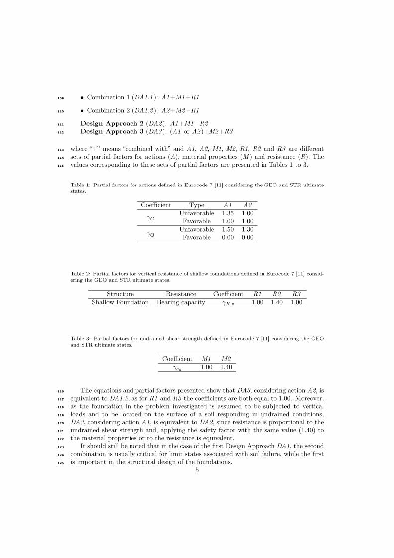
values corresponding to these sets of partial factors are presented in Tables 1 to 3.115
Table 1: Partial factors for actions defined in Eurocode 7 [11] considering the GEO and STR ultimatestates.
Coefficient Type A1 A2
γGUnfavorable 1.35 1.00Favorable 1.00 1.00
γQUnfavorable 1.50 1.30Favorable 0.00 0.00
Table 2: Partial factors for vertical resistance of shallow foundations defined in Eurocode 7 [11] consid-ering the GEO and STR ultimate states.
Structure Resistance Coefficient R1 R2 R3Shallow Foundation Bearing capacity γR,v 1.00 1.40 1.00
Table 3: Partial factors for undrained shear strength defined in Eurocode 7 [11] considering the GEOand STR ultimate states.
Coefficient M1 M2γcu 1.00 1.40
The equations and partial factors presented show that DA3, considering action A2, is116
equivalent to DA1.2, as for R1 and R3 the coefficients are both equal to 1.00. Moreover,117
as the foundation in the problem investigated is assumed to be subjected to vertical118
loads and to be located on the surface of a soil responding in undrained conditions,119
DA3, considering action A1, is equivalent to DA2, since resistance is proportional to the120
undrained shear strength and, applying the safety factor with the same value (1.40) to121
the material properties or to the resistance is equivalent.122
It should still be noted that in the case of the first Design Approach DA1, the second123
combination is usually critical for limit states associated with soil failure, while the first124
is important in the structural design of the foundations.125
5
Consequently, in the following text, only DA1.2 and DA2 will be analyzed, and, for126
the present case, the only difference between DA1.2 and DA2 is the partial safety factor127
applied to actions (A1 vs. A2 ).128
It is common practice in some countries to consider a Design Approach DA2* instead129
of DA2, where the effects of actions are factored instead of the actions themselves. This130
DA2* was, however, not considered in the present paper.131
4. Finite element modeling132
The foundation analyzed in the present work represents a continuous footing with133
width B, equal to 1 m, and subjected to a vertical load F . The footing was considered134
rigid and rough. The foundation soil was modeled with dimensions equal to 5B × 2B,135
in accordance with the dimensions of soil modeled in [22, 23]. Vertical and horizontal136
displacements on the base of the mesh and on its left and right sides were restrained.137
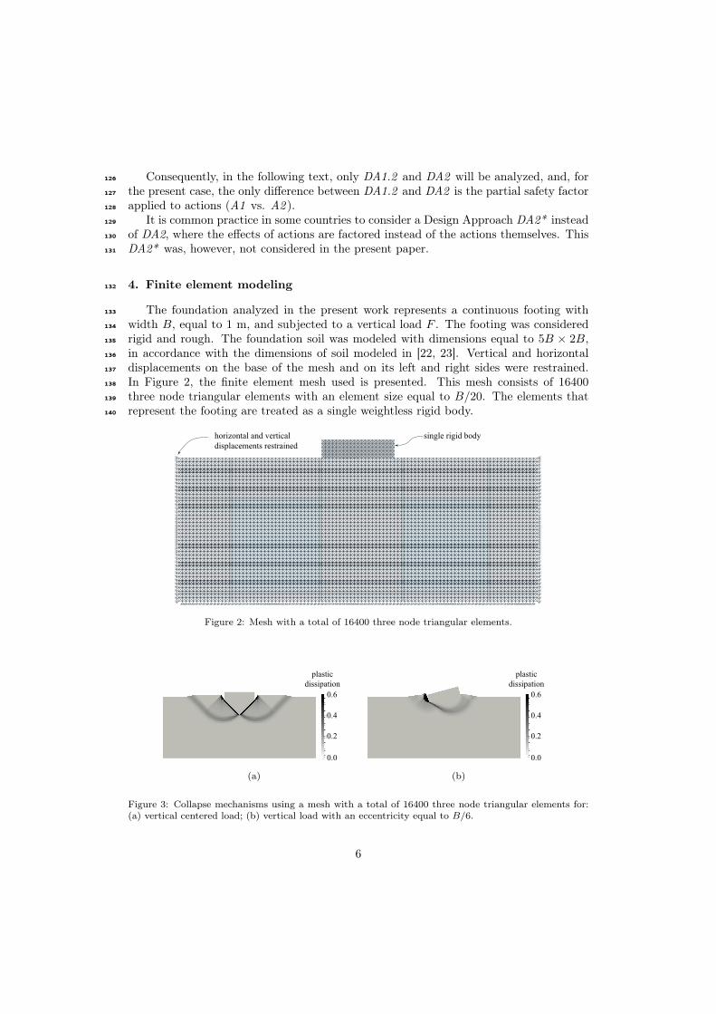
In Figure 2, the finite element mesh used is presented. This mesh consists of 16400138
three node triangular elements with an element size equal to B/20. The elements that139
represent the footing are treated as a single weightless rigid body.140
single rigid bodyhorizontal and vertical
displacements restrained
Figure 2: Mesh with a total of 16400 three node triangular elements.
plastic
dissipation
0.0
0.2
0.4
0.6
(a)
plastic
dissipation
0.0
0.2
0.4
0.6
(b)
Figure 3: Collapse mechanisms using a mesh with a total of 16400 three node triangular elements for:(a) vertical centered load; (b) vertical load with an eccentricity equal to B/6.
6
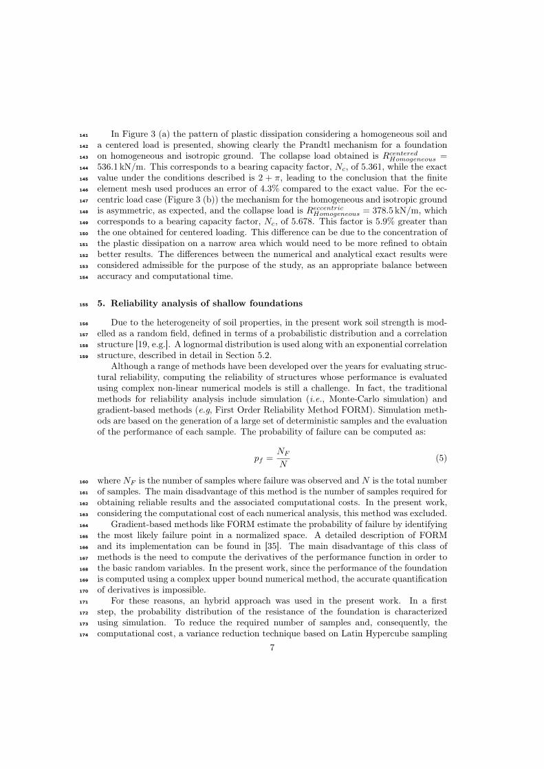
In Figure 3 (a) the pattern of plastic dissipation considering a homogeneous soil and141
a centered load is presented, showing clearly the Prandtl mechanism for a foundation142
on homogeneous and isotropic ground. The collapse load obtained is RcenteredHomogeneous =143
536.1 kN/m. This corresponds to a bearing capacity factor, Nc, of 5.361, while the exact144
value under the conditions described is 2 + π, leading to the conclusion that the finite145
element mesh used produces an error of 4.3% compared to the exact value. For the ec-146
centric load case (Figure 3 (b)) the mechanism for the homogeneous and isotropic ground147
is asymmetric, as expected, and the collapse load is ReccentricHomogeneous = 378.5 kN/m, which148
corresponds to a bearing capacity factor, Nc, of 5.678. This factor is 5.9% greater than149
the one obtained for centered loading. This difference can be due to the concentration of150
the plastic dissipation on a narrow area which would need to be more refined to obtain151
better results. The differences between the numerical and analytical exact results were152
considered admissible for the purpose of the study, as an appropriate balance between153
accuracy and computational time.154
5. Reliability analysis of shallow foundations155
Due to the heterogeneity of soil properties, in the present work soil strength is mod-156
elled as a random field, defined in terms of a probabilistic distribution and a correlation157
structure [19, e.g.]. A lognormal distribution is used along with an exponential correlation158
structure, described in detail in Section 5.2.159
Although a range of methods have been developed over the years for evaluating struc-tural reliability, computing the reliability of structures whose performance is evaluatedusing complex non-linear numerical models is still a challenge. In fact, the traditionalmethods for reliability analysis include simulation (i.e., Monte-Carlo simulation) andgradient-based methods (e.g, First Order Reliability Method FORM). Simulation meth-ods are based on the generation of a large set of deterministic samples and the evaluationof the performance of each sample. The probability of failure can be computed as:
pf =NF
N(5)
where NF is the number of samples where failure was observed and N is the total number160
of samples. The main disadvantage of this method is the number of samples required for161
obtaining reliable results and the associated computational costs. In the present work,162
considering the computational cost of each numerical analysis, this method was excluded.163
Gradient-based methods like FORM estimate the probability of failure by identifying164
the most likely failure point in a normalized space. A detailed description of FORM165
and its implementation can be found in [35]. The main disadvantage of this class of166
methods is the need to compute the derivatives of the performance function in order to167
the basic random variables. In the present work, since the performance of the foundation168
is computed using a complex upper bound numerical method, the accurate quantification169
of derivatives is impossible.170
For these reasons, an hybrid approach was used in the present work. In a first171
step, the probability distribution of the resistance of the foundation is characterized172
using simulation. To reduce the required number of samples and, consequently, the173
computational cost, a variance reduction technique based on Latin Hypercube sampling174
7
was employed. Based on the results of the simulation process, a probability distribution175
was fit to the sampled foundation resistance. This allows the definition of the limit state176
function as the difference between the resistance and the effect of the applied loads. This177
is a simple analytical expression, and FORM can be used to compute the probability of178
failure.179
5.1. Simulation of random fields180
As described above, simulation can be used to generate random fields of the undrained181
shear strength and, finally, compute the probabilistic distribution of the collapse load.182
In this work, the random field was discretized using the mid-point method [30], i.e., the183
space was discretized in stochastic elements and a constant value of the undrained shear184
strength was adopted for each stochastic mesh element. This method produces a relation185
between the random field and a set of correlated random variables. Simulation can then186
be used to generate samples of the random variables and, consequently, of the associated187
random field.188
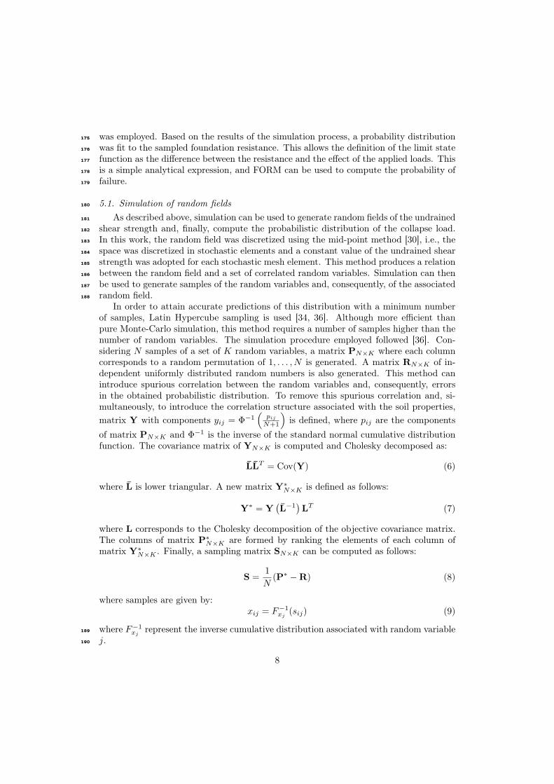
In order to attain accurate predictions of this distribution with a minimum numberof samples, Latin Hypercube sampling is used [34, 36]. Although more efficient thanpure Monte-Carlo simulation, this method requires a number of samples higher than thenumber of random variables. The simulation procedure employed followed [36]. Con-sidering N samples of a set of K random variables, a matrix PN×K where each columncorresponds to a random permutation of 1, . . . , N is generated. A matrix RN×K of in-dependent uniformly distributed random numbers is also generated. This method canintroduce spurious correlation between the random variables and, consequently, errorsin the obtained probabilistic distribution. To remove this spurious correlation and, si-multaneously, to introduce the correlation structure associated with the soil properties,matrix Y with components yij = Φ−1
(pij
N+1
)is defined, where pij are the components
of matrix PN×K and Φ−1 is the inverse of the standard normal cumulative distributionfunction. The covariance matrix of YN×K is computed and Cholesky decomposed as:
L̄L̄T = Cov(Y) (6)
where L̄ is lower triangular. A new matrix Y∗N×K is defined as follows:
Y∗ = Y(L̄−1
)LT (7)
where L corresponds to the Cholesky decomposition of the objective covariance matrix.The columns of matrix P∗N×K are formed by ranking the elements of each column ofmatrix Y∗N×K . Finally, a sampling matrix SN×K can be computed as follows:
S =1
N(P∗ −R) (8)
where samples are given by:xij = F−1xj
(sij) (9)
where F−1xjrepresent the inverse cumulative distribution associated with random variable189
j.190
8

5.2. Probabilistic characterization of soil191
In general, the lognormal distribution is adequate to model material strengths [26].192
In the case of soil properties, it is particularly useful, since variability can be very large193
[38], but only positive values have physical meaning [22, 6]. For these reasons, and in194
accordance with previous works [22, 23, 28], the undrained shear strength was defined as195
a lognormal distribution.196
The correlation between the soil properties in two points can be modelled consideringan autocorrelation function, in terms of the vertical and horizontal distance betweenthe two points [52, 19]. In the present work, an ellipsoidal exponential autocorrelationfunction [52, 19] was used for the logarithm of the undrained shear strength:
ρlncu(∆V ,∆H) = exp
−√√√√(2|∆V |
θVln cu
)2
+
(2|∆H |θHln cu
)2 (10)
where θVln cuand θHln cu
are the vertical and horizontal spatial correlation lengths, respec-197
tively, and ∆V and ∆H are the vertical and horizontal distances between the two points.198
If both spatial correlation lengths are equal, the spatial correlation structure is isotropic199
and, otherwise, anisotropic.200
The spatial correlation length, or fluctuation scale, describes the homogeneity of soil,201
defining a distance above which the correlation is lower than a given value [50, 52].202
A high value of the correlation length implies a more homogeneous soil, with softer203
variations of the undrained shear strength . The correlation lengths can be replaced204
by a dimensionless parameter, denoted spatial correlation, defined as Θln cu = θln cu/B205
[22, 19], where B is the foundation width. Then, the vertical and horizontal correlation206
lengths can be defined in terms of the dimensionless spatial correlations, ΘVln cu
= θVln cu/B207
and ΘHln cu
= θHln cu/B.208
In this work, the mean undrained shear strength will be assumed constant and equal209
to 100 kPa. Considering the values proposed in literature [33, 51, 5, 31, 24, 47, 12, 40,210
42, 38, 39, 14, 6, e.g.] for the mean value of the coefficient of variation and horizontal and211
vertical spatial correlation length of the undrained shear strength, the following values212
are assumed in the present work for these parameters:213
CVcu = {0.125; 0.25; 0.5; 1}214
ΘVln cu
= {0.5; 1; 2; 4; 8}215
ΘHln cu
= {1.0ΘVln cu
; 10ΘVln cu}216
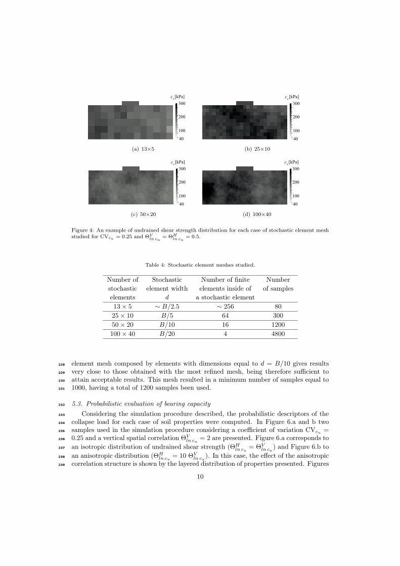
The heterogeneity of the soil is modelled considering the domain divided in a quadran-217
gular stochastic element mesh. In the generation of the samples for soil properties, four218
stochastic element meshes with different levels of refinement were studied as described219
in Table 4, with the objective of defining the minimum refinement, and, consequently,220
the minimum number of samples, required to ensure the correct soil spatial variabil-221
ity modelling. For this study, an isotropic spatial correlation structure was considered222
(ΘHln cu
= ΘVln cu
), as well as a vertical centered load. In Figure 4, an example for each223
stochastic element mesh is presented, considering CVcu = 0.25 and ΘVln cu
= ΘHln cu
= 0.5.224
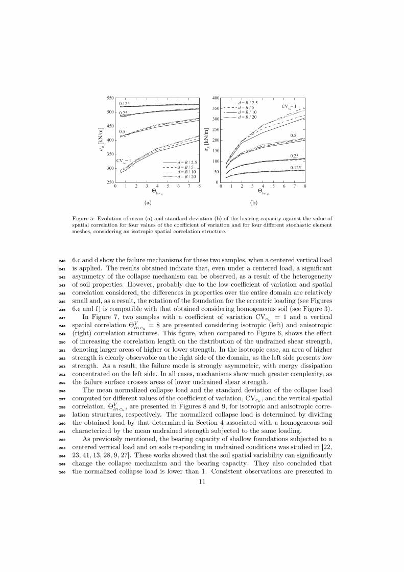
Figure 5 shows the mean and the standard deviation of the collapse load computed225
for different values of the coefficient of variation, CVcu , and of the spatial correlation,226
ΘVln cu
for the four different stochastic element meshes. Results show that a stochastic227
9
cu [kPa]
40
100
200
300
(a) 13×5
cu [kPa]
40
100
200
300
(b) 25×10
cu [kPa]
40
100
200
300
(c) 50×20
cu [kPa]
40
100
200
300
(d) 100×40
Figure 4: An example of undrained shear strength distribution for each case of stochastic element meshstudied for CVcu = 0.25 and ΘV
ln cu= ΘH
ln cu= 0.5.
Table 4: Stochastic element meshes studied.
Number of Stochastic Number of finite Numberstochastic element width elements inside of of sampleselements d a stochastic element13× 5 ∼ B/2.5 ∼ 256 8025× 10 B/5 64 300
50× 20 B/10 16 1200
100× 40 B/20 4 4800
element mesh composed by elements with dimensions equal to d = B/10 gives results228
very close to those obtained with the most refined mesh, being therefore sufficient to229
attain acceptable results. This mesh resulted in a minimum number of samples equal to230
1000, having a total of 1200 samples been used.231
5.3. Probabilistic evaluation of bearing capacity232
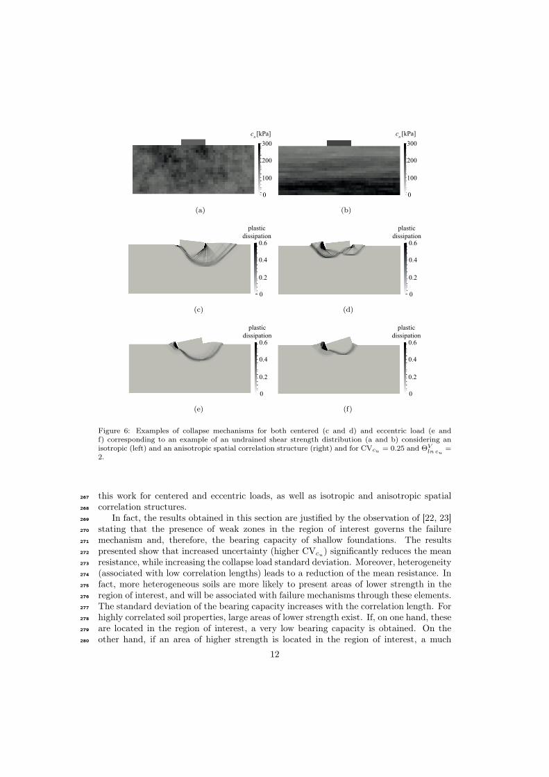
Considering the simulation procedure described, the probabilistic descriptors of the233
collapse load for each case of soil properties were computed. In Figure 6.a and b two234
samples used in the simulation procedure considering a coefficient of variation CVcu =235
0.25 and a vertical spatial correlation ΘVln cu
= 2 are presented. Figure 6.a corresponds to236
an isotropic distribution of undrained shear strength (ΘHln cu
= ΘVln cu
) and Figure 6.b to237
an anisotropic distribution (ΘHln cu
= 10 ΘVln cu
). In this case, the effect of the anisotropic238
correlation structure is shown by the layered distribution of properties presented. Figures239
10
0 1 2 3 4 5 6 7 8250
300
350
400
450
500
550
Θln c
µR [kN/m]
d = B / 2.5d = B / 5d = B / 10d = B / 20
CVc = 1
0.5
0.25
0.125
u
u
(a)
0 1 2 3 4 5 6 7 80
50
100
150
200
250
300
350
400
Θln c
σR [
kN
/m]
u
d = B / 2.5d = B / 5d = B / 10d = B / 20
CVc = 1u
0.5
0.25
0.125
(b)
Figure 5: Evolution of mean (a) and standard deviation (b) of the bearing capacity against the value ofspatial correlation for four values of the coefficient of variation and for four different stochastic elementmeshes, considering an isotropic spatial correlation structure.
6.c and d show the failure mechanisms for these two samples, when a centered vertical load240
is applied. The results obtained indicate that, even under a centered load, a significant241
asymmetry of the collapse mechanism can be observed, as a result of the heterogeneity242
of soil properties. However, probably due to the low coefficient of variation and spatial243
correlation considered, the differences in properties over the entire domain are relatively244
small and, as a result, the rotation of the foundation for the eccentric loading (see Figures245
6.e and f) is compatible with that obtained considering homogeneous soil (see Figure 3).246
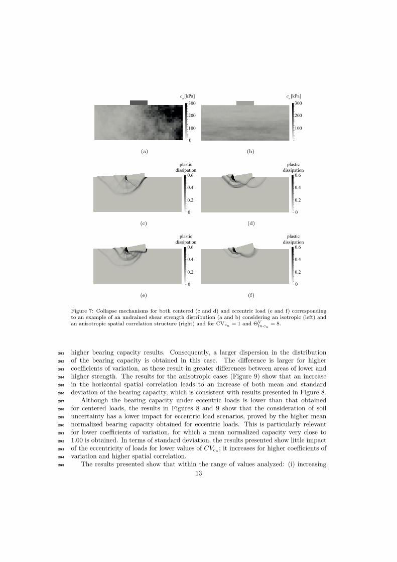
In Figure 7, two samples with a coefficient of variation CVcu = 1 and a vertical247
spatial correlation ΘVln cu
= 8 are presented considering isotropic (left) and anisotropic248
(right) correlation structures. This figure, when compared to Figure 6, shows the effect249
of increasing the correlation length on the distribution of the undrained shear strength,250
denoting larger areas of higher or lower strength. In the isotropic case, an area of higher251
strength is clearly observable on the right side of the domain, as the left side presents low252
strength. As a result, the failure mode is strongly asymmetric, with energy dissipation253
concentrated on the left side. In all cases, mechanisms show much greater complexity, as254
the failure surface crosses areas of lower undrained shear strength.255
The mean normalized collapse load and the standard deviation of the collapse load256
computed for different values of the coefficient of variation, CVcu , and the vertical spatial257
correlation, ΘVln cu
, are presented in Figures 8 and 9, for isotropic and anisotropic corre-258
lation structures, respectively. The normalized collapse load is determined by dividing259
the obtained load by that determined in Section 4 associated with a homogeneous soil260
characterized by the mean undrained strength subjected to the same loading.261
As previously mentioned, the bearing capacity of shallow foundations subjected to a262
centered vertical load and on soils responding in undrained conditions was studied in [22,263
23, 41, 13, 28, 9, 27]. These works showed that the soil spatial variability can significantly264
change the collapse mechanism and the bearing capacity. They also concluded that265
the normalized collapse load is lower than 1. Consistent observations are presented in266
11
cu [kPa]
0
100
200
300
(a)
cu [kPa]
0
100
200
300
(b)
plastic
dissipation
0
0.2
0.4
0.6
(c)
plastic
dissipation
0
0.2
0.4
0.6
(d)
plastic
dissipation
0
0.2
0.4
0.6
(e)
plastic
dissipation
0
0.2
0.4
0.6
(f)
Figure 6: Examples of collapse mechanisms for both centered (c and d) and eccentric load (e andf) corresponding to an example of an undrained shear strength distribution (a and b) considering anisotropic (left) and an anisotropic spatial correlation structure (right) and for CVcu = 0.25 and ΘV
ln cu=
2.
this work for centered and eccentric loads, as well as isotropic and anisotropic spatial267
correlation structures.268
In fact, the results obtained in this section are justified by the observation of [22, 23]269
stating that the presence of weak zones in the region of interest governs the failure270
mechanism and, therefore, the bearing capacity of shallow foundations. The results271
presented show that increased uncertainty (higher CVcu) significantly reduces the mean272
resistance, while increasing the collapse load standard deviation. Moreover, heterogeneity273
(associated with low correlation lengths) leads to a reduction of the mean resistance. In274
fact, more heterogeneous soils are more likely to present areas of lower strength in the275
region of interest, and will be associated with failure mechanisms through these elements.276
The standard deviation of the bearing capacity increases with the correlation length. For277
highly correlated soil properties, large areas of lower strength exist. If, on one hand, these278
are located in the region of interest, a very low bearing capacity is obtained. On the279
other hand, if an area of higher strength is located in the region of interest, a much280
12
cu [kPa]
0
100
200
300
(a)
cu [kPa]
100
200
300
(b)
plastic
dissipation
0
0.2
0.4
0.6
(c)
plastic
dissipation
0
0.2
0.4
0.6
(d)
plastic
dissipation
0
0.2
0.4
0.6
(e)
plastic
dissipation
0
0.2
0.4
0.6
(f)
Figure 7: Collapse mechanisms for both centered (c and d) and eccentric load (e and f) correspondingto an example of an undrained shear strength distribution (a and b) considering an isotropic (left) andan anisotropic spatial correlation structure (right) and for CVcu = 1 and ΘV
ln cu= 8.
higher bearing capacity results. Consequently, a larger dispersion in the distribution281
of the bearing capacity is obtained in this case. The difference is larger for higher282
coefficients of variation, as these result in greater differences between areas of lower and283
higher strength. The results for the anisotropic cases (Figure 9) show that an increase284
in the horizontal spatial correlation leads to an increase of both mean and standard285
deviation of the bearing capacity, which is consistent with results presented in Figure 8.286
Although the bearing capacity under eccentric loads is lower than that obtained287
for centered loads, the results in Figures 8 and 9 show that the consideration of soil288
uncertainty has a lower impact for eccentric load scenarios, proved by the higher mean289
normalized bearing capacity obtained for eccentric loads. This is particularly relevant290
for lower coefficients of variation, for which a mean normalized capacity very close to291
1.00 is obtained. In terms of standard deviation, the results presented show little impact292
of the eccentricity of loads for lower values of CVcu ; it increases for higher coefficients of293
variation and higher spatial correlation.294
The results presented show that within the range of values analyzed: (i) increasing295
13
0 1 2 3 4 5 6 7 80.5
0.6
0.7
0.8
0.9
1.0
centered
eccentric
Θln c
µR
,iso
trop
ic / R
Hom
ogeneo
us
u
CVc = 1u
0.5
0.125
0.25
(a)
0 1 2 3 4 5 6 7 80
50
100
150
200
250
300
350
400
centered
eccentric
σR
,iso
tro
pic [
kN
/m] CV
c = 1u
0.5
0.125
0.25
Θln cu
(b)
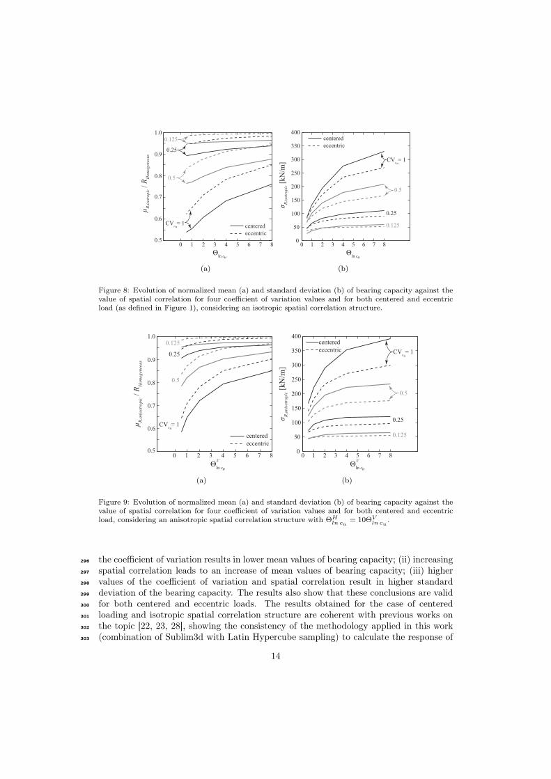
Figure 8: Evolution of normalized mean (a) and standard deviation (b) of bearing capacity against thevalue of spatial correlation for four coefficient of variation values and for both centered and eccentricload (as defined in Figure 1), considering an isotropic spatial correlation structure.
0 1 2 3 4 5 6 7 8
centered
Θln cu
V
0.5
0.6
0.7
0.8
0.9
1.0
µR
,anis
otr
opic / R
Hom
ogeneous
CVc = 1u
0.5
0.125
0.25
eccentric
(a)
centered
eccentric
0.125
0.25
0.5
0 1 2 3 4 5 6 7 80
50
100
150
200
250
300
350
400
σR
,anis
otr
opic [
kN
/m]
CVc = 1u
Θln cu
V
(b)
Figure 9: Evolution of normalized mean (a) and standard deviation (b) of bearing capacity against thevalue of spatial correlation for four coefficient of variation values and for both centered and eccentricload, considering an anisotropic spatial correlation structure with ΘH
ln cu= 10ΘV
ln cu.
the coefficient of variation results in lower mean values of bearing capacity; (ii) increasing296
spatial correlation leads to an increase of mean values of bearing capacity; (iii) higher297
values of the coefficient of variation and spatial correlation result in higher standard298
deviation of the bearing capacity. The results also show that these conclusions are valid299
for both centered and eccentric loads. The results obtained for the case of centered300
loading and isotropic spatial correlation structure are coherent with previous works on301
the topic [22, 23, 28], showing the consistency of the methodology applied in this work302
(combination of Sublim3d with Latin Hypercube sampling) to calculate the response of303
14
shallow foundations.304
0 1 2 3 4 5 6 7
0.5
0.125
centered - anisotr.
eccentric - anisotr.
centered - isotr.
eccentric - isotr.CVc = 1u
0.5
0.6
0.7
0.8
0.9
1.0
Θln c
µR
,iso
tropic /
RH
om
ogeneous
u
V8
(a)
0 1 2 3 4 5 6 7 80
50
100
150
200
250
300
350
400
σR [
kN
/m]
Θln cu
V
CVc = 1u
0.5
0.125
(b)
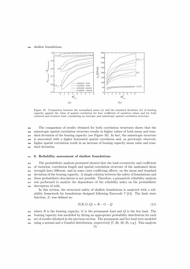
Figure 10: Comparison between the normalized mean (a) and the standard deviation (b) of bearingcapacity against the value of spatial correlation for four coefficient of variation values and for bothcentered and eccentric load, considering an isotropic and anisotropic spatial correlation structure.
The comparison of results obtained for both correlation structures shows that the305
anisotropic spatial correlation structure results in higher values of both mean and stan-306
dard deviation of the bearing capacity (see Figure 10). In fact, the anisotropic structure307
is associated with a higher horizontal spatial correlation and, as previously observed,308
higher spatial correlation result in an increase of bearing capacity mean value and stan-309
dard deviation.310
6. Reliability assessment of shallow foundations311
The probabilistic analysis presented showed that the load eccentricity and coefficient312
of variation, correlation length and spatial correlation structure of the undrained shear313
strength have different, and in some cases conflicting effects, on the mean and standard314
deviation of the bearing capacity. A simple relation between the safety of foundations and315
these probabilistic descriptors is not possible. Therefore, a parametric reliability analysis316
was performed to analyse the dependence of the reliability index on the probabilistic317
descriptors of soils.318
In this section, the structural safety of shallow foundations is analyzed with a reli-ability framework for foundations designed following Eurocode 7 [11]. The limit statefunction, Z, was defined as:
Z(R,G,Q) = R−G−Q (11)
where R is the bearing capacity, G is the permanent load and Q is the live load. The319
bearing capacity was modelled by fitting an appropriate probability distribution for each320
set of results obtained in the previous section. The permanent and live load were modeled321
using a normal and a Gumbel distribution, respectively [7, 26, 49, 25, e.g.]. This analysis322
15
presents a practical interest as it evaluates the consistency of the partial safety factors323
method, currently prescribed in Eurocode 7[11].324
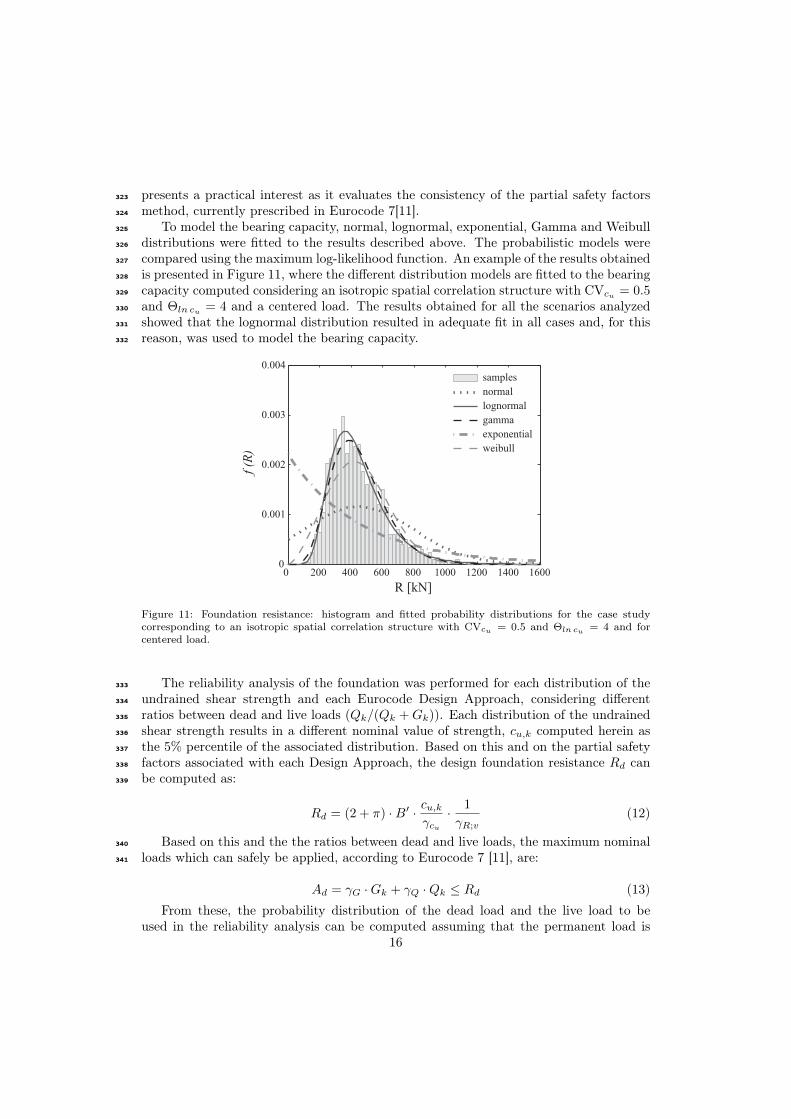
To model the bearing capacity, normal, lognormal, exponential, Gamma and Weibull325
distributions were fitted to the results described above. The probabilistic models were326
compared using the maximum log-likelihood function. An example of the results obtained327
is presented in Figure 11, where the different distribution models are fitted to the bearing328
capacity computed considering an isotropic spatial correlation structure with CVcu = 0.5329
and Θln cu = 4 and a centered load. The results obtained for all the scenarios analyzed330
showed that the lognormal distribution resulted in adequate fit in all cases and, for this331
reason, was used to model the bearing capacity.332
0 200 400 600 800 1000 1200 1400 1600 0
0.001
0.002
0.003
0.004
R [kN]
f (R
)
samples
normal
lognormal
gamma
exponential
weibull
Figure 11: Foundation resistance: histogram and fitted probability distributions for the case studycorresponding to an isotropic spatial correlation structure with CVcu = 0.5 and Θln cu = 4 and forcentered load.
The reliability analysis of the foundation was performed for each distribution of the333
undrained shear strength and each Eurocode Design Approach, considering different334
ratios between dead and live loads (Qk/(Qk +Gk)). Each distribution of the undrained335
shear strength results in a different nominal value of strength, cu,k computed herein as336
the 5% percentile of the associated distribution. Based on this and on the partial safety337
factors associated with each Design Approach, the design foundation resistance Rd can338
be computed as:339
Rd = (2 + π) ·B′ · cu,kγcu· 1
γR;v(12)
Based on this and the the ratios between dead and live loads, the maximum nominal340
loads which can safely be applied, according to Eurocode 7 [11], are:341
Ad = γG ·Gk + γQ ·Qk ≤ Rd (13)
From these, the probability distribution of the dead load and the live load to beused in the reliability analysis can be computed assuming that the permanent load is
16
characterized by a normal distribution with a coefficient of variation equal to 10% whilethe live load can be modeled appropriately by a Gumbel distribution with a coefficient ofvariation equal to 35% [7, 26, 49, 25, e.g.]. If all variables were independent and normallydistributed, the reliability index could be computed as:
β = Φ−1(pf ) =µR − µG − µQ√σ2R + σ2
G + σ2Q
(14)
where µR, µG and µQ are the mean of the normal distribution which characterize the342
resistance, permanent load and live load, respectively, and σR, σG and σQ are the cor-343
respondent standard deviations. In the present case, as the variables are non-Gaussian,344
this expression results only in an estimate of the reliability index. Consequently, the re-345
liability index was computed using iForm [48], implemented in the open-source program346
FERUM (Finite Element Reliability Using Matlab) [8, 29].347
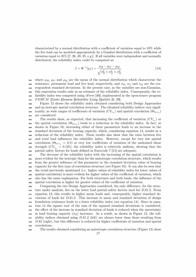
Figure 12 shows the reliability index obtained considering both Design Approaches348
and an isotropic spatial correlation structure. The obtained reliability indices vary signif-349
icantly, as wide ranges of coefficients of variation (CVcu) and spatial correlation (Θln cu)350
are considered.351
The results show, as expected, that increasing the coefficient of variation (CVcu) or352
the spatial correlation (Θln cu) leads to a reduction in the reliability index. In fact, as353
shown in Figure 10, increasing either of these parameters leads to an increase in the354
standard deviation of the bearing capacity, which, considering equation 14, results in a355
reduction of the reliability index. These results also show that the ratio between live356
and total load influences the reliability index. However, except for very low spatial357
correlation (Θln cu = 0.5) or very low coefficients of variation of the undrained shear358
strength (CVcu = 0.125), the reliability index is relatively uniform, showing that the359
partial safety factors for loads defined in Eurocode 7 [11] are adequate.360
The decrease of the reliability index with the increasing of the spatial correlation is361
more evident for the isotropic than for the anisotropic correlation structure, which results362
from the greater influence of this parameter in the standard deviation value of bearing363
capacity for the first type of correlation structure (see Figure 10). It can also be seen that364
the trend previously mentioned (i.e. higher values of reliability index for lower values of365
spatial correlation) is more evident for higher values of the coefficient of variation, which366
also has the same explanation. For both structures and both loads, the influence of the367
spatial correlation is higher for greater values of the coefficient of variation.368
Comparing the two Design Approaches considered, the only difference, for the struc-369
ture under analysis, lies on the lower load partial safety factors used for DA1.2. From370
equation 13, this results in higher mean loads and, consequently, higher standard de-371
viations of loads for DA1.2. This increase in mean and standard deviation of design372
foundation resistance leads to a lower reliability index (see equation 14). Since in equa-373
tion 14 the square root of the sum of the squared standard deviations is considered,374
the effect of the increase in standard deviation of loads is reduced when the uncertainty375
in load bearing capacity (σR) increases. As a result, as shown in Figure 12, the reli-376
ability indices obtained using DA1.2 (left) are always lower than those resulting from377
DA2 (right), but this difference is reduced for higher coefficients of variation and spatial378
correlations.379
The results obtained considering an anisotropic correlation structure (Figure 13) show380
17
centered
eccentric
homogeneous case
1 0
Qk / (G
k +Q
k) Q
k / (G
k +Q
k)
Qk / (G
k +Q
k) Q
k / (G
k +Q
k)
Qk / (G
k +Q
k) Q
k / (G
k +Q
k)
Θln c
=0.5u
u
u
V
2
8
Θln c
=0.5u
V
2
8
Θln c
=0.5u
V
2
8
8
Θln c
=0.5V
2
8
Θln c
=0.5V
uΘ
ln c =0.5
V
2
8
2
0 0.2 0.4 0.6 0.8 0.2 0.4 0.6 0.8
0 0.2 0.4 0.6 0.8 1 0 0.2 0.4 0.6 0.8 1
1
1 0 0.2 0.4 0.6 0.8 0 0.2 0.4 0.6 0.8 1 4
5
6
7
8
9
10
3
4
5
6
7
8
9
2
3
4
5
6
7
8
ββ
β
(a) (b)
(c) (d)
(e) (f)
3.6
3.6 3.6
3.6
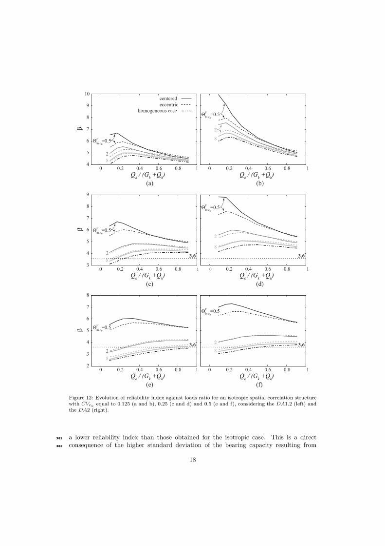
Figure 12: Evolution of reliability index against loads ratio for an isotropic spatial correlation structurewith CVcu equal to 0.125 (a and b), 0.25 (c and d) and 0.5 (e and f), considering the DA1.2 (left) andthe DA2 (right).
a lower reliability index than those obtained for the isotropic case. This is a direct381
consequence of the higher standard deviation of the bearing capacity resulting from382
18
4
5
6
7
8
3
4
5
6
7
2
3
4
5
6
centered
eccentric
homogeneous case
1 0
Qk / (G
k +Q
k) Q
k / (G
k +Q
k)
Qk / (G
k +Q
k) Q
k / (G
k +Q
k)
Qk / (G
k +Q
k) Q
k / (G
k +Q
k)
0 0.2 0.4 0.6 0.8 0.2 0.4 0.6 0.8
0 0.2 0.4 0.6 0.8 1 0 0.2 0.4 0.6 0.8 1
1
1 0 0.2 0.4 0.6 0.8 0 0.2 0.4 0.6 0.8 1
ββ
β
(a) (b)
(c) (d)
(e) (f)
Θln c
=0.5u
V
2
2
8
Θln c
=0.5u
V
28
Θln c
=0.5u
V
28
Θln c
=0.5u
V
28
Θln c
=0.5u
V
28
8
Θln c
=0.5u
V
3.6 3.6
3.6 3.6
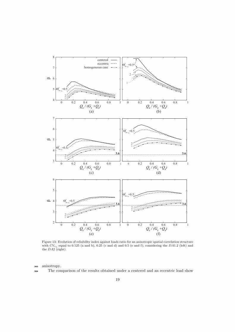
Figure 13: Evolution of reliability index against loads ratio for an anisotropic spatial correlation structurewith CVcu equal to 0.125 (a and b), 0.25 (c and d) and 0.5 (e and f), considering the DA1.2 (left) andthe DA2 (right).
anisotropy.383
The comparison of the results obtained under a centered and an eccentric load show384
19
very small differences, indicating that the approach used in Eurocode 7 [11] for assessing385
the safety of eccentric loaded shallow foundations is consistent.386
In Figures 12 and 13, the reliability index obtained assuming a homogeneous soil387
(θln cu → ∞) and an analytical limit state function are also presented. In all examples388
analyzed, assuming a homogeneous soil leads to lower safety levels, as a result of the389
increase in bearing capacity standard deviation. Therefore, analytical models assuming390
homogeneous soil can be regarded as a simple but conservative approach to the safety391
analysis of shallow foundation.392
Comparing the reliability indices computed with the threshold defined in Eurocode393
0 [10] (βtarget = 3.6), it can be seen that DA2 leads to acceptable safety levels, except394
if lower values of live load to total load ratios, high coefficient of variation and spatial395
correlation are considered for the undrained shear strength. On the other hand, the396
use of Design Approach DA1.2 leads to undesirable safety levels for a wide range of397
probabilistic soil properties, presenting the same trends as seen for the Design Approach398
DA2.399
7. Conclusions400
In the present work a reliability assessment of shallow foundations subjected to ver-401
tical loads, responding in undrained conditions, considering explicitly the soil spatial402
variability was carried out. Firstly, random fields representing the soil, considering dif-403
ferent coefficients of variation, both vertical and horizontal spatial correlation lengths and404
soil spatial correlation structure were generated using Latin Hypercube sampling. Re-405
garding to the shallow foundations bearing capacity response, it is important to highlight406
that:407
• the mean value of the bearing capacity increases with decreasing coefficients of vari-408
ation and increasing spatial correlation lengths. The standard deviation value of409
the bearing capacity increases with increasing coefficients of variation and spatial410
correlation lengths. These trends were observed for both centered and eccentric411
loadings, as well as isotropic and anisotropic distributions of the spatial variability.412
These observations are consistent with previous works focusing on the same topic413
[22, 23, 41, 13, 28, 9, 27], which confirms that the combination of the Latin Hyper-414
cube sampling [34, 36] with Sublim3d [45] is suitable to investigate the influence of415
soil heterogeneity in the bearing capacity of foundations [46];416
• the ratio between the mean value of the bearing capacity and the bearing capacity417
value determined considering a homogeneous soil is similar for centered and eccen-418
tric loads. Regarding to the standard deviation, the values obtained tend to be419
smaller for the eccentric load;420
• the results obtained for an anisotropic spatial correlation structure are consistent421
with those expected when there is an increase in the spatial correlation length,422
i.e., comparing the results obtained for both spatial correlation structures, greater423
values of mean and standard deviation values of the bearing capacity are verified424
for the anisotropic structure (for the same vertical scale of fluctuation).425
20
With the bearing capacity response reliability index following Eurocode 7 [11] ap-426
proaches were calculated based on iForm [48] implemented on the open-source program427
FERUM [8]. With respect to the results obtained for the reliability index, the main428
conclusions are:429
• DA2 leads always to larger values of reliability index as consequence of its greater430
values for partial safety factors;431
• DA1.2 leads to undesirable safety levels for a wide range of probabilistic soil prop-432
erties, presenting, nevertheless, the same trends as seen for the Design Approach433
DA2;434
• the difference between the two approaches will increase if the base of the foundation435
is below the surface, as is usually the case in practice;436
• the results have shown very small differences between centered and eccentric load;437
• the approach used in Eurocode 7 [11] for assessing the safety of eccentric loaded438
shallow foundations is consistent;439
• for the cases analysed in the present work, reliability analysis using analytical440
models assuming homogeneous soil can be regarded as a simple but conservative441
approach to the safety analysis of shallow foundations;442
Acknowledgments443
The authors acknowledge the support of the Geotechnical Group of the Department of444
Civil Engineering of the Universidade Nova de Lisboa and UNIC - Centro de Investigação445
em Estruturas e Construção. The second author acknowledges the support of Fundação446
para a Ciência e Tecnologia through grant PTDC/ECM/115932/2009.447
References448
[1] Ahmed, A., Soubra, A.H.: Probabilitstic analysis of strip footings resting on a spatially random449
soil using subset simulation approach. Georisk 6, 188–201 (2012)450
[2] Ahmed, A., Soubra, A.H.: Probabilitstic analysis at serviceability limit state of two neigboring strip451
footings resting on a spatially random soil. Structural Safety 49, 2–9 (2014)452
[3] Al-Bittar, T., Soubra, A.H.: Probabilistic analysis of strip footings resting on spatially varying453
soils and subjected to vertical or inclined loads. Journal of Geotechnical and Geoenvironmental454
Engineering 140(4) (2014)455
[4] Antão, A.N., Vicente da Silva, M., Guerra, N.M.C., Delgado, R.: An upper bound-based solution456
for the shape factors of bearing capacity of footings under drained conditions using a parallelized457
mixed f.e. formulation with quadratic velocity fields. Computers and Geotechnics 41, 23–35 (2012)458
[5] Asoaka, A., Grivas, D.: Spatial variability of the undrained strength of clays. Journal of Engineering459
Mechanics 108(5), 743–756 (1982). ASCE460
[6] Baecher, G.B., Christian, J.T.: Reliability and Statistics in Geotechnical Engineering. John Wiley461
and Sons (2003)462
[7] Bartlett, F.M., Hong, H.P., Zhou, W.: Load factor calibration for the proposed 2005 edition of the463
national building code of canada: Statistics of loads and load effects. Canadian Journal of Civil464
Engineering 30(2), 429–439 (2003)465
[8] Bourinet, J.M.: Ferum 4.1 user’s guide (2010)466
[9] Cassidy, M.J., Uzielli, M., Tian, Y.: Probabilistic combined loading failure envelopes of a strip467
footing on spatially variable soil. Computers and Geotechnics 49, 191–205 (2013)468
21
[10] CEN: EN 1990:2009, Eurocode 0 - Basis of structural design. European Committee for Standard-469
ization (2009)470
[11] CEN: EN 1997-1:2010, Eurocode 7 - Geotechnical design. European Committee for Standardization471
(2010)472
[12] Chiasson, P., Lafleur, J., Soulié, M., Law, K.T.: Characterizing spatial variability of a clay by473
geostatistics. Canadian Geotechnical Journal 32, 1–10 (1995)474
[13] Cho, S.E., Park, H.C.: Effect of spatial variability of cross-correlated soil properties on bearing475
capacity of strip footing. International Journal for Numerical and Analytical Methods in Geome-476
chanics 34, 1–26 (2010)477
[14] Duncan, J.M.: Factors of safety and reliability in geotechnical engineering. Journal of Geotechnical478
and Geoenvironmental Engineering 126, 307–316 (2000)479
[15] Fenton, G.A.: Simulation and analysis of random fields. Ph.D. thesis, Department of Civil Engi-480
neering and Operations Research, Princeton University (1990)481
[16] Fenton, G.A.: Error evaluation of three random-field generators. Journal of engineering mechanics482
120(12), 2478–2497 (1994)483
[17] Fenton, G.A., Griffiths, D.V.: Probabilistic foundation settlement on a spatially random soil. Jour-484
nal of Geotechnical and Geoenvironmental Engineering 128(5), 381–390 (2002). ASCE485
[18] Fenton, G.A., Griffiths, D.V.: Three−dimensional probabilistic foundation settlement. Journal of486
Geotechnical and Geoenvironmental Engineering 131(2), 232–239 (2005). ASCE487
[19] Fenton, G.A., Griffiths, D.V.: Risk Assessment in Geotechnical Engineering. John Wiley and Sons,488
New York (2008)489
[20] Fenton, G.A., Vanmarcke, E.: Simulation of random fields via local average subdivision. Journal of490
Engineering Mechanics 116(8), 1733–1749 (1990). ASCE491
[21] Florian, A.: An efficient sampling scheme: Updated latin hypercube sampling. Probabilistic Engi-492
neering Mechanics 7, 123–130 (1992)493
[22] Griffiths, D.V., Fenton, G.A.: Bearing capacity of spatially random soil: the undrained clay prandtl494
problem revisited. Géotechnique 51(4), 351–359 (2001)495
[23] Griffiths, D.V., Fenton, G.A., Manoharan, N.: Bearing capacity of rough rigid strip footing on496
cohesive soil: Probabilistic study. ASCE Journal Geotechnical and Geoenvironmental Engineering497
128(9), 743–755 (2002)498
[24] Harr, M.E.: Reliability based design in civil engineering. McGraw Hill, London, New York (1987)499
[25] Holicky, V., Markova, J., Gulvanessian, H.: Code calibration allowing for reliability differentia-500
tion and production quality. In: Application of Statistics and Probability in Civil Engineering:501
Proceedings of the 10th International Conference. Kanda, Takada and Furuat (2007)502
[26] JCSS: JCSS Probabilistic Model Code. Part 2: Load Models. Joint Commitee on Structural Safety503
(2001)504
[27] Jha, S.: Reliability-based analysis of bearing capacity of strip footings considering anisotropic505
correlation of spatially varying undrained shear strength. International Journal of Geomechanics506
(2016)507
[28] Kasama, K., Whittle, A.J.: Bearing capacity of spatially random cohesive soil using numerical limit508
analyses. Journal of Geotechnical and Geoenvironmental Engineering 137(11), 989–996 (2011)509
[29] Kiureghian, A.D., Haukaas, T., Fujimura, K.: Structural reliability software at the university of510
california, berkeley. Structural Safety 28(1), 44–67 (2006)511
[30] Kiureghian, A.D., Ke, J.B.: The stochastic finite element method in structural reliability. Proba-512
bilistic Engineering Mechanics 3(2), 83–91 (1988)513
[31] Lee, I., White, W., Ingles, O.: Geotechnical Engineering. Pitman, London (1983)514
[32] Low, B.K., Phoon, K.K.: Reliability-based design and its complementary role to eurocode 7 design515
approach. Computers and Geotechnics 65, 30–44 (2015)516
[33] Lumb, P.: The variability of natural soils. Canadian Geotechnical Journal 3, 74–97 (1966)517
[34] McKay, M.D., Beckman, R.J., Conover, W.J.: A comparison of three methods for selecting values518
of input variables in the analysis of output from a computer code. Technometrics 21(2), 239–245519
(1979)520
[35] Melchers, R.E., Beck, A.T.: Structural reliability analysis and prediction. John Wiley & Sons521
(2018)522
[36] Olsson, A., Sandberg, G., Dahlblom, O.: On latin hypercube sampling for structural reliability523
analysis. Structural Safety 25(1), 47–68 (2003)524
[37] Paice, G.M., Griffiths, D.V., Fenton, G.A.: Finite element modeling of settlements on spatially525
random soil. Journal of Geotechnical Engineering 122(9), 777–779 (1996)526
[38] Phoon, K.K., Kulhawy, F.H.: Characterization of geotechnical variability. Canadian Geotechnical527
22
Journal 36(3), 612–624 (1999)528
[39] Phoon, K.K., Kulhawy, F.H.: Evaluation of geotechnical property variability. Canadian Geotech-529
nical Journal 36(3), 625–639 (1999)530
[40] Popescu, R.: Stochastic variability of soil properties: data analysis, digital simulation, effects on531
system behaviour. Ph.D. thesis, Princeton University, USA (1995)532
[41] Popescu, R., Deodatis, G., Nobahar, A.: Effects of random heterogeneity of soil properties on533
bearing capacity. Probabilistic Engineering Mechanics 20(4), 324–341 (2005)534
[42] Popescu, R., Prevost, J.H., Deodatis, G.: Effects of spatial variability on soil liquefaction: some535
design recommendations. Géotechnique 47, 1019–1036 (1997)536
[43] Vicente da Silva, M.: Implementação numérica tridimensional do teorema cinemático da análise537
limite. Ph.D. thesis, Faculdade de Ciências e Tecnologia da Universidade Nova de Lisboa, Lisboa538
(2009). In Portuguese539
[44] Vicente da Silva, M., Antão, A.N.: A non-linear programming method approach for upper bound540
limit analysis. International Journal for Numerical Methods in Engineering 72, 1192–1218 (2007)541
[45] Vicente da Silva, M., Antão, A.N.: Upper bound limit analysis with a parallel mixed finite element542
formulation. International Journal of Solids and Structures 45, 5788–5804 (2008)543
[46] Simões, J.T., Neves, L.C., Antão, A.N., Guerra, N.M.C.: Probabilistic analysis of bearing capacity544
of shallow foundations using three-dimensional limit analyses. International Journal of Computa-545
tional Methods 11(2), 1342,008–1–20 (2014)546
[47] Soulié, M., Montes, M., Silvestri, V.: Modelling spatial variability of soil parameters. Canadian547
Geotechnical Journal 27, 617–630 (1990)548
[48] Sudret, B., Kiureghian, A.D.: Stochastic Finite Element Methods and Reliability, A State-of-the-549
Art Report. Department of Civil and Environmental Engineering, University of California, Berkeley550
(2000)551
[49] Teixeira, A., Correia, A.G., Honjo, Y., Henriques, A.A.: Reliability analysis of a pile foundation in552
a residual soil: contribution of the uncertainties involved and partial factors. In: 3rd International553
Symposium on Geotechnical Safety and Risk (ISGSR2011). Munich, Germany: Vogt, Schuppener,554
Straub and Bräu (2011)555
[50] Vanmarcke, E.: Probabilistic modeling of soil profiles. Journal of the Geotechnical Engineering556
Division 103(11), 1227–1246 (1977). ASCE557
[51] Vanmarcke, E.: Reliability of earth slopes. Journal of the Geotechnical Engineering Division558
103(11), 1247–1265 (1977). ASCE559
[52] Vanmarcke, E.: Random Fields: Analysis and Synthesis. Princeton University, USA (2010)560
[53] Whitman, R.V.: Organizing and evaluating uncertainty in geotechnical engineering. Journal of561
Geotechnical and Geoenvironmental Engineering 126(7), 583–593 (2000)562
23


