Embed Size (px)
Citation preview

REMOTE SENSING OF THE ELECTRODYNAMIC
COUPLING BETWEEN THUNDERSTORM SYSTEMS
AND THE MESOSPHERE / LOWER IONOSPHERE
a dissertation
submitted to the department of electrical engineering
and the committee on graduate studies
of stanford university
in partial fulfillment of the requirements
for the degree of
doctor of philosophy
By
Steven Craig Reising
June 1998

c© Copyright 1998 by Steven Craig Reising
All Rights Reserved
ii


Dedication
In Memoriam
Flavian “Flip” Reising(1912-1997)
M. Elizabeth “Betty” Reising(1910-1988)
Joseph P. Bradley(1895-1968)
J. Theresia Bradley(1901-1981)
For the love and labor of those who preceded us,
May we deserve their legacy.
iv

Abstract
In the past few years, dramatic experimental evidence has emerged, showing that
tropospheric lightning discharges modify the mesosphere and the lower ionosphere
through heating and ionization, producing gamma-ray bursts and optical emissions
known as red sprites, blue jets, and elves. These transient electrodynamic coupling
processes may have long-term effects such as chemical changes, persistent heating
of ionospheric electrons, and increased production of mesospheric and stratospheric
nitrogen oxides (NOy). In order to assess the regional and global effects of the intense
electrodynamic coupling of thunderstorms to the middle atmosphere, the occurrence
rate of Sprites needs to be known over large areas of the Earth. Since continuous
optical monitoring of Sprite occurrence on large spatial scales is not practical, a
continuous proxy indicator for Sprite occurrence is needed.
Sprites are intense, transient luminous events in the mesosphere and lower iono-
sphere above thunderstorm systems. They extend from ∼40 to ∼90 km in altitude, are
primarily red in color, and develop to full brightness in a few milliseconds. Sprites
are nearly uniquely associated with positive cloud-to-ground lightning flashes, yet
they occur in association with only a small subset of those flashes. The peak cur-
rent of each flash, measured at high frequencies by the National Lightning Detection
Network, is not a sufficient indicator of the likelihood of a positive cloud-to-ground
lightning flash to produce a Sprite.
In this work, remote sensing of the electrodynamic coupling between thunderstorm
systems and the mesosphere and lower ionosphere is accomplished by measurement
of radio atmospherics in the ELF (extremely low frequency, here 15 Hz - 1.5 kHz) and
VLF (very low frequency, here 1.5 - 22 kHz) ranges. Radio atmospherics (“sferics”)
provide a unique signature of each lightning return stroke and propagate efficiently in
the waveguide bounded by the Earth’s surface and the ionosphere. Novel digital sig-
nal processing techniques for ELF/VLF broadband measurements allow automated
v

detection and arrival azimuth determination of individual radio atmospherics. Ar-
rival azimuth measurement is accomplished with ±1 precision for radio atmospher-
ics propagating from Nebraska to Palmer Station, Antarctica, a source-to-receiver
distance of ∼12,000 km. Identification of the time of occurrence of sferics to ∼1-
millisecond precision allows the identification of individual lightning discharges as
the source of individual radio atmospherics. Broadband ELF/VLF measurements of
radio atmospherics therefore allow the determination of characteristics of those light-
ning discharges which couple strongly to the middle atmosphere and lead to Sprite
production.
Broadband measurements of sferics performed near Ft. Collins, Colorado, ∼500
km from the causative lightning, demonstrate that the ELF sferic energy is a proxy
indicator which can be used to estimate the number of Sprites produced by a thun-
derstorm with an accuracy of ±25%. In addition, simultaneous video observations of
Sprites reveal variable delays of up to 100 milliseconds between the positive cloud-
to-ground flash and Sprite onset. Comparison with high-resolution photometer mea-
surements demonstrate the simultaneity of Sprite luminosity and an ELF “second
pulse,” radiated by electrical currents within the Sprite body [Cummer et al., 1998].
Measurements of the second pulse are used to identify a quantitative relationship
between the current in Sprites and total Sprite luminosity. Ultra-long range measure-
ments at Palmer Station, Antarctica, show that Sprite-associated sferics have large
ELF magnitudes in relation to non Sprite-associated sferics as measured at a range
of ∼12,000 km [Reising et al., 1996]. These results suggest that a few appropriately
placed ELF/VLF sferics receivers may be sufficient for estimation of global Sprite
occurrence rates.
vi

Acknowledgements
Near the middle of this work, I realized that the proverbial had become true; I was and
am standing on the shoulders of giants. Our accomplishments would be impossible
without the legacy of our predecessors and the guidance and collaboration of our
contemporaries. The least I can do is to recognize some of the persons who have
participated in this work and in my development as a scientist and as an engineer.
First and foremost, I would like to express my unequivocal gratitude to Professor
Umran Inan, my principal advisor, for leading me into the field and the fray of
scientific inquiry, for showing me by example how to succeed as a researcher and a
scholar, and for supporting and promoting our efforts with seemingly boundless energy
and dedication. Secondly, I would like to give wholehearted thanks to Dr. Tim Bell,
my co-advisor, for his cheerful guidance in the development of a discerning eye and
mind and for his ever-present wit and insight in facing our everyday challenges in
the world of science. Professor Bob Helliwell passed along to me, as to so many,
the original enthusiasm and inquisitiveness with which he founded the VLF Group
more than forty years ago. Dr. Vikas Sonwalkar provided initial advice on the subject
of sferics and continuing encouragement as his career took him to the University of
Alaska Fairbanks. Professor Don Carpenter was a continual source of encouragement
and support. I thank Professor Tony Fraser-Smith for his scientific discussions, for
serving on my orals committee and for his first-rate sense of humor. I give special
thanks to Professor J. W. Goodman for serving as my orals chairman and third reader
of this dissertation.
The staff of the VLF Group made this work possible. Shao Lan Min and June
Wang provided outstanding proposal support and cheerful advice. Bill Trabucco
gave me unparalleled training on field work in the Arctic and Antarctic regions and
on building reliable, fail-safe hardware. Jerry Yarbrough taught me time-saving and
vii
essential techniques for broadband data analysis. Dr. Ev Paschal contributed indis-
pensible engineering designs of the broadband receivers deployed both at Yucca Ridge
and at Palmer Station.
Many graduates of the VLF Group contributed to my training. Dr. Dave Shafer
introduced me to the fundamental skills of engineering design for reliability and gave
me important advice on everything from negotiations with sponsors to travel in Chile.
Dr. Bill Burgess provided data analysis software and many helpful hints on success as a
Ph.D. student. Dr. Juan Rodriguez gave me guidance and encouragement during our
three years as office mates. Darren Hakeman passed along excellent software for digital
signal processing. Dr. Steve Cummer provided the 60 Hz removal algorithm and sferic
viewing software. Finally, as both a student and a postdoctoral scholar, Dr. Victor
Pasko provided many invaluable discussions on lightning and the electrodynamics of
Sprites.
Current VLF Group students have contributed to this work. Chris Barrington-
Leigh helped with analysis and interpretation of video and photometric data. Mike
Johnson contributed Matlab algorithms and analysis ideas. Sean Lev-Tov and Dave
Lauben expertly managed the computers, and Nikolai Lehtinen answered my inces-
sant questions about Adobe Illustrator software. Several undergraduate students,
principally Jason Deng and Ayse Inan, contributed countless hours of analysis of
sferics waveforms.
Many from outside the STAR Laboratory played important roles in the develop-
ment of this work. Professor Dave Sentman of the University of Alaska Fairbanks
served as a mentor, guide and motivator through engaging scientific discussions in di-
verse places from Trapper Creek, Alaska, to Mont Saint-Michel, France. Dr. Martin
Fullekrug, whom Tony Fraser-Smith recruited for postdoctoral work at Stanford, was
outstanding in his encouragement, dedication and willingness to provide collabora-
tion. Dr. James Weinman of NASA Goddard Space Flight Center provided continual
enthusiasm for our subject and outstanding mentoring during my summer at Goddard
and in the years which followed.
I would like to thank Dr. Walt Lyons and Tom Nelson of FMA Research, Inc., for
hosting and assisting in our experiments at Yucca Ridge, Colorado, and for insights
on Great Plains meteorology and “Sprite forecasts.” John Booth hosted my 1994
visit to Palmer Station, Antarctica, which proved to be one of the highlights of my
graduate career. Since then, John Booth, Kevin Bliss and Glenn Grant have provided
viii

talented and dedicated support for the Palmer Station experiments which provided
much of the data for this dissertation.
In closing, I cannot forget the people that play the most pivotal role in all of our
lives, our families. I am grateful to my parents, Flavian and Mary Jo, for teaching
me the value of education, of committing myself to a goal and of persisting to achieve
it. I thank my sister, Kathy, for her unflagging love and support. Finally, my wife
Kathleen Zaleski has been the most patient and the most steadfast in her belief in
my potential for success. For all of these giants in my life, I am forever grateful.
Steven C. Reising
Stanford, CaliforniaMay 31, 1998
This research was made possible by the people of the United States through the
sponsorship of the National Aeronautics and Space Administration (NASA) under
grant NGT-30281 to Stanford University, a NASA Graduate Student Fellowship in
Earth Systems Science. Data acquisition at Palmer Station, Antarctica, was spon-
sored by the National Science Foundation through grants OPP-9318596 and OPP-
96115855 to Stanford University. Observations at Yucca Ridge Field Station, Col-
orado, were supported by the Air Force Research Laboratory under grant F19628-96-
C-0075 and by the Office of Naval Research under AASERT grant N00014-95-1-1095.
ix

Contents
Dedication iv
Abstract v
Acknowledgements vii
1 Introduction 1
1.1 Sprites . . . . . . . . . . . . . . . . . . . . . . . . . . . . . . . . . . . 2
1.2 Lightning Discharges and Thunderstorm Systems . . . . . . . . . . . 4
1.2.1 Positive and Negative Discharges . . . . . . . . . . . . . . . . 4
1.2.2 Continuing Currents . . . . . . . . . . . . . . . . . . . . . . . 5
1.2.3 Global Lightning . . . . . . . . . . . . . . . . . . . . . . . . . 7
1.2.4 The National Lightning Detection Network . . . . . . . . . . . 8
1.2.5 Mesoscale Convective Systems . . . . . . . . . . . . . . . . . . 9
1.3 Radio Atmospherics . . . . . . . . . . . . . . . . . . . . . . . . . . . . 12
1.4 Contributions of this Work . . . . . . . . . . . . . . . . . . . . . . . . 14
2 Broadband ELF/VLF Lightning Detection and Location 15
2.1 Broadband ELF/VLF Receiving Systems . . . . . . . . . . . . . . . . 16
2.1.1 ELF/VLF Receiver at Palmer Station, Antarctica . . . . . . . 17
2.1.2 ELF/VLF Sferic Receiver at Yucca Ridge, Colorado . . . . . . 19
2.2 Sferic Detection . . . . . . . . . . . . . . . . . . . . . . . . . . . . . . 20
2.3 Sferic Arrival Azimuth Determination . . . . . . . . . . . . . . . . . . 23
2.4 Precision of Sferic Arrival Azimuth Determination . . . . . . . . . . . 24
3 Association of Sprites and Cloud-to-Ground Lightning 30
3.1 Identification of Sprite Onset Time . . . . . . . . . . . . . . . . . . . 30
x

3.2 Association of Sprites and Positive Cloud-to-Ground Flashes . . . . . 32
3.3 Delays between Positive CG Flashes and Sprite Onsets . . . . . . . . 36
4 ELF Sferic Energy as a Proxy Indicator for Sprite Occurrence 39
4.1 Quantitative Analysis of VLF and ELF sferics . . . . . . . . . . . . . 41
4.2 Medium Range Measurements at Yucca Ridge, Colorado . . . . . . . 44
4.3 Ultra-Long Range Measurements at Palmer Station, Antarctica . . . 47
4.3.1 Continuing Currents in Sprite-Associated Lightning Flashes . 48
4.3.2 Sprite-Producing Storm on July 12, 1994 . . . . . . . . . . . . 49
4.3.3 Sprite-Producing Storm on July 15, 1995 . . . . . . . . . . . . 51
4.3.4 Application of ELF Proxy to Multiple Storms . . . . . . . . . 52
4.4 ELF Radiation from Electrical Currents in Sprites . . . . . . . . . . . 54
5 Summary and Suggestions for Future Work 65
5.1 Summary . . . . . . . . . . . . . . . . . . . . . . . . . . . . . . . . . 65
5.2 Suggestions for Future Work . . . . . . . . . . . . . . . . . . . . . . . 67
5.2.1 Assessment of the Global Distribution of Sprite Occurrence . . 67
5.2.2 ELF/VLF Proxy Indicator for the Occurrence of Elves . . . . 68
5.2.3 Multistation Measurements of Global Lightning Flash Rates . 69
Bibliography 72
xi

List of Tables
2.1 Comparison of Palmer and Yucca Ridge broadband systems . . . . . 19
xii

List of Figures
1.1 Image of a Sprite recorded at ∼550 km range on July 24, 1996. . . . . 2
1.2 Worldwide lightning flash density observations by the Optical Tran-
sient Detector orbiting at 750 km altitude and 70 inclination. . . . . 7
1.3 Bipolar structure of an Oklahoma winter thunderstorm. . . . . . . . . 10
1.4 Schematic of electrification of mesoscale convective systems, including
positive CGs and horizontal discharges in the stratiform region. . . . 11
2.1 ELF/VLF sferic data analysis block diagram. . . . . . . . . . . . . . 16
2.2 ELF/VLF sferic receiver block diagram. . . . . . . . . . . . . . . . . 17
2.3 Palmer Station broadband ELF/VLF receiver frequency response. . . 18
2.4 Yucca Ridge broadband ELF/VLF sferic receiver frequency response. 20
2.5 Spectrogram of broadband data showing noise background, as mea-
sured at Palmer Station, Antarctica. . . . . . . . . . . . . . . . . . . 21
2.6 Map of great circle paths from North America to Palmer Station,
Antarctica, a range of ∼12,000 km. . . . . . . . . . . . . . . . . . . . 25
2.7 Map of NLDN-detected positive CG lightning flashes in the western
U.S. on August 1, 1996. . . . . . . . . . . . . . . . . . . . . . . . . . 26
2.8 Magnitude and arrival direction spectrograms for VLF data recorded
at Palmer Station, with simultaneous NLDN data. . . . . . . . . . . . 27
2.9 Sferics histogram as function of both VLF peak intensity and arrival
azimuth at Palmer Station on August 1, 1996. . . . . . . . . . . . . . 28
2.10 Error histogram demonstrating arrival azimuth determination to ±1 at
Palmer Station. . . . . . . . . . . . . . . . . . . . . . . . . . . . . . . 29
3.1 Determination of Sprite onset time from video observations. . . . . . 31
3.2 NLDN lightning locations and camera field of view of western Kansas
thunderstorm from Yucca Ridge, Colorado . . . . . . . . . . . . . . . 34
xiii

3.3 Time delays between positive cloud-to-ground flashes and Sprite onsets. 37
4.1 Removal of power line interference from sferics data recorded at Yucca
Ridge, Colorado. . . . . . . . . . . . . . . . . . . . . . . . . . . . . . 42
4.2 Measurement of the VLF and ELF components of sferics recorded at
Yucca Ridge, Colorado. . . . . . . . . . . . . . . . . . . . . . . . . . . 43
4.3 Histogram of the NLDN-recorded peak current for Sprite-associated
and non Sprite-associated sferics on August 1, 1996. . . . . . . . . . . 45
4.4 Histogram of the ELF sferic energy for Sprite-associated and non Sprite-
associated sferics on August 1, 1996. . . . . . . . . . . . . . . . . . . 46
4.5 Histogram showing the use of ELF sferic energy as a proxy indicator
for Sprite occurrence. . . . . . . . . . . . . . . . . . . . . . . . . . . . 47
4.6 Palmer Station sferics waveforms which have similar VLF peak inten-
sity but widely differing ELF slow-tail magnitudes. . . . . . . . . . . 48
4.7 Maps of NLDN-recorded positive CG flash locations and Sprite-associated
flashes on July 12, 1994, and July 15, 1995. . . . . . . . . . . . . . . . 50
4.8 Histograms of NLDN peak current and ELF sferic energy in comparison
with Sprite occurrence for July 12, 1994. . . . . . . . . . . . . . . . . 51
4.9 Histograms of NLDN peak current and ELF sferic energy in comparison
with Sprite occurrence for July 15, 1995. . . . . . . . . . . . . . . . . 52
4.10 Histograms of NLDN peak current and ELF sferic energy for multiple
storms in comparison with Sprite occurrence on August 1, 1996. . . . 53
4.11 Infrared brightness temperature measured on the GOES 8 satellite on
August 1, 1996. . . . . . . . . . . . . . . . . . . . . . . . . . . . . . . 55
4.12 Comparison of sferics waveforms with and without the second ELF pulse. 56
4.13 Simultaneous ELF second pulse and photometer measurements of Sprite
luminosity at 08:24:00 UT on August 1, 1996. . . . . . . . . . . . . . 57
4.14 Simultaneous ELF second pulse and photometer measurements of Sprite
luminosity at 08:39:30 UT on August 1, 1996. . . . . . . . . . . . . . 58
4.15 Linear relationship between Sprite charge moment and total Sprite
luminosity for 17 Sprites on July 24, 1996. . . . . . . . . . . . . . . . 59
4.16 Broadband sferics data measured at Yucca Ridge on July 24, 1996,
showing ∼56-ms delay between the first and second ELF pulses. . . . 60
xiv

4.17 Simultaneous multi-anode photometer and broadband ELF data for
the Sprite-associated sferic shown in Figure 4.16. . . . . . . . . . . . . 61
4.18 Broadband sferics data measured at Yucca Ridge on July 24, 1996,
showing ∼70-ms delay between the first and second ELF pulses. . . . 62
4.19 Simultaneous multi-anode photometer and broadband ELF data for
the Sprite-associated sferic shown in Figure 4.18. . . . . . . . . . . . . 63
4.20 Relationship between continuing current charge moment and CG-to-
Sprite delay for 17 Sprites on July 24, 1996. . . . . . . . . . . . . . . 64
xv

Chapter 1
Introduction
Each lightning discharge dissipates a total energy of ∼109 J, of which ∼106 J is radi-
ated as electromagnetic energy, during a duration of ∼0.1 ms [Uman, 1987; pp. 322-
323]. Energy released by a subset of lightning discharges couples to the mesosphere
and the lower ionosphere, where the most dramatic visible effects are transient, lu-
minous glows known as Sprites (see Figure 1.1), first recorded in 1989 [Franz et al.,
1990]. The characteristics of Sprites are described in Section 1.1. Each Sprite ap-
pears following a positive cloud-to-ground lightning discharge [Boccippio et al., 1995;
Reising et al., 1996]. The characteristics of lightning discharges and the thunderstorm
systems relevant to Sprites are described in Section 1.2. The intensity of the lightning
discharge, which is measured routinely by the National Lightning Detection Network,
is not a sufficient indicator of whether or not a given positive discharge is likely to
initiate a Sprite. In this work, lightning discharges are remotely characterized via the
measurement of their electromagnetic signatures, known as radio atmospherics, which
propagate efficiently in the Earth-ionosphere waveguide. Measurement of radio atmo-
spherics allows detection of the properties of those lightning discharges which lead to
Sprites and, consequently, of the total number of Sprites produced by a thunderstorm.
The characteristics of radio atmospherics are described in Section 1.3.
1

CHAPTER 1. INTRODUCTION 2
1.1 Sprites
Sprites are transient luminous glows in the middle atmosphere above thunderstorms,
arguably the most dramatic visible evidence of electrodynamic coupling between thun-
derstorm systems and the overlying mesosphere and lower ionosphere (see Figure 1.1).
Sprites extend from ∼40 to ∼90 km in altitude and have transverse extents of ∼10
to ∼50 km [Sentman et al., 1995; Lyons, 1996]. They develop to full brightness in
1-3 ms [Cummer et al., 1998], but their luminosity may last for 10-100 ms [Fukunishi
et al., 1996; Winckler et al., 1996; Lyons, 1996]. Low light level video observations of
Sprites have been conducted from the Space Shuttle [Boeck et al., 1995], from aircraft
[Sentman and Wescott, 1993; Sentman et al., 1995] and from the ground [Franz et
al., 1990; Lyons, 1994; 1996; Winckler et al., 1996].
0 10 20 30 40 Distance (km)
90
80
70
60
50
40
Altitude (km)
24 Jul 9604:09:19.553 UT
sprite
clouds
horizon
Figure 1.1: Image of a Sprite recorded by an intensified CCD video camera at Yucca Ridge,Colorado, at ∼550 km range. Observations were made as a part of the Stanford University Fly’sEye Experiment.
Observations of other optical emissions provide additional evidence of electrody-
namic coupling between thunderstorm systems and the middle atmosphere, including
blue jets and blue starters from aircraft [Wescott et al., 1995; 1996] and elves from the
Space Shuttle [Boeck et al., 1992] and from the ground [Fukunishi et al., 1996; Inan

CHAPTER 1. INTRODUCTION 3
et al., 1997]. Other evidence of electrodynamic coupling includes VLF signatures of
rapid changes in conductivity and ionization in the lower ionosphere [Inan et al., 1988,
1993, 1995, 1996a; Dowden et al., 1994] and radar detection of transient ionization
patches above a thunderstorm [Roussel-Dupre and Blanc, 1997]. The observation of
terrestrial gamma-ray flashes by the Burst and Transient Source Experiment is one
of the most unexpected discoveries made by the Compton Gamma-Ray Observatory
[Fishman et al., 1994]. A number of satellite observations of gamma-ray flashes have
been directly associated with individual sferics generated by positive CG discharges
[Inan et al., 1996b]. The gamma-ray photon energy extends above 1 MeV, indicating
bremsstrahlung radiation from >1 MeV electrons, consistent with predictions of up-
ward beams of runaway electrons accelerated by thundercloud electric fields [Wilson,
1925; Bell et al., 1995; Taranenko and Roussel-Dupre, 1996; Lehtinen et al., 1996;
1997].
Sprites are believed to be produced by intense quasi-electrostatic fields (tens of
kV/m at ∼70 km altitude) which exist at high altitudes following positive CG dis-
charges [Pasko et al., 1995, 1996, 1997; Boccippio et al., 1995; Winckler et al., 1996;
Fernsler and Rowland, 1996]. These quasi-electrostatic fields lead to ambient electron
heating (up to ∼5 eV average energy), the ionization of neutrals and the excitation
of optical emissions in the altitude range ∼40 to ∼90 km [Pasko et al., 1997, and
references therein]. The runaway electron mechanism may also play a role in Sprite
generation [Bell et al., 1995; Taranenko and Roussel-Dupre, 1996; Lehtinen et al.,
1996; 1997]. Another mechanism of interaction with the mesosphere and the lower
ionosphere is the heating of ambient electrons by lightning electromagnetic pulses,
which has been applied to explain the existence of elves [Inan et al., 1991, 1996c;
Taranenko et al., 1993; Rowland et al., 1995, 1996] and of Sprites [Milikh et al.,
1995].
For the quasi-electrostatic mechanism of Sprite production, the important param-
eters that determine whether or not a positive CG flash produces a Sprite are the
altitude and magnitude of the thundercloud charge removed to ground. For a fixed al-
titude of removed charge, the single most important parameter in determining Sprite
occurrence is the magnitude of the charge lowered to ground. The discharge duration
plays a secondary role, as long as the charge removal time is shorter than the local
relaxation time (εo/σ) at ∼70-90 km altitudes [Boccippio et al., 1995; Pasko et al.,
1995; 1997].

CHAPTER 1. INTRODUCTION 4
1.2 Lightning Discharges and Thunderstorm
Systems
In this dissertation we consider primarily cloud-to-ground (CG) lightning discharges,
as opposed to intracloud discharges, which do not make electrical contact with the
ground. This focus is appropriate because Sprites are nearly exclusively accompanied
by CG flashes. In fact, the vast majority of prior research on lightning has also focused
on CG discharges because of their potential for damage to property and living things,
and because of their relative accessibility for study. It should be noted, however, that
the number of intracloud discharges in a thunderstorm exceeds the number of CG
discharges by a factor of ∼2-5 [Uman, 1987; pp. 44-45], and that the energy released
in intracloud discharges may play an important role in electrodynamic coupling to
the middle and upper atmosphere.
1.2.1 Positive and Negative Discharges
The polarity of a CG lightning discharge is classified as “positive” or “negative” based
on the polarity of its net effect on the charge of the thundercloud. If the net effect of
the discharge is to move negative charge (electrons) from the cloud to the ground, it
is called a negative CG. If it has the net effect of transferring positive charge from the
cloud to the ground (electrons moving upward), then it is called a positive CG. This
terminology is in common use in the lightning literature [Uman, 1987; pp. 9-10]. The
total CG discharge is called a flash and has a typical duration of 0.1 - 1 s. A CG flash
consists of a series of leaders, typically three or four, each followed by return strokes,
which occur each time there is a completion of the electrical connection between
the cloud’s charge reservoir and the ground. The first return stroke is initiated by
the stepped leader, the visible channel following a high conductivity path formed by
preliminary breakdown preceding the flash. If the flash ends when the first return
stroke ceases, it is called a single-stroke flash. On the other hand, if additional charge
is available in the cloud, a dart leader may propagate down the residual channel and
initiate a subsequent return stroke. As many as 15 more return strokes may occur
in the same flash, with typical delays between strokes of 30-100 ms [Uman, 1987;
pp. 10-19].
Negative and positive CGs differ in their properties and occurrence rates. Positive

CHAPTER 1. INTRODUCTION 5
flashes are generally composed of a single stroke, sometimes followed by a period
of continuing current (see Section 1.2.2). Positive CGs may dominate some winter
storms, reportedly constituting up to 90-100% of the total lightning [Brook et al, 1989].
However, overall lightning rates in winter are low, and summer thunderstorms produce
predominantly negative CG flashes [Uman, 1987; p. 20]. Consequently, negatives
represented >97% of the CG flashes in the continental U.S. during 1989-1991, as
recorded by the National Lightning Detection Network (see Section 1.2.4) [Orville,
1994]. An increase in the fraction of positive lightning in summer thunderstorms
is correlated with increasing latitude and with increasing elevation above sea level
[Uman, 1987; p. 20].
One of the most complete descriptions of return stroke currents is based on mea-
surements of discharges to towers in Switzerland (e.g., [Berger et al., 1975]). The
currents were derived from measurements of the voltages induced in resistive shunts
located on two towers reaching 55 m above the summit of Mt. San Salvatore [Uman,
1987; p. 120]. Based on these measurements, the average duration of negative first
return strokes is ∼0.1 ms. The duration of positive first return strokes has more
variability, with an average value of 0.2-0.6 ms [Berger et al., 1975]. However, their
recorded waveforms may have been altered by the electrical characteristics of the
tower and measuring circuit and by the difference between discharges to tall objects
and discharges to ground [Uman, 1987; p. 121]. Peak current magnitudes measured
by Berger et al. [1975] were observed to fit a log-normal distribution. Negative first
return strokes had a median peak current of 20-40 kA, with levels of 200 kA reached
only 1% of the time. Subsequent return strokes carried approximately half the peak
current of first strokes. Positive return strokes exhibited the same median peak cur-
rent as first return strokes, but in extreme cases were much larger, with 5% of the
positive peak currents exceeding 250 kA [Uman, 1987; pp. 122-125].
1.2.2 Continuing Currents
The total charge lowered from a thundercloud at a given altitude to the ground in a
lightning discharge is believed to be the most important parameter in determining its
potential for producing a Sprite (see Section 1.1 and [Pasko et al., 1997]). The charge
lowered to ground can be computed by integrating the current waveform over time.
Typical values of charge transfer in the <0.1 ms duration of a negative return stroke

CHAPTER 1. INTRODUCTION 6
are ∼3-5 C for first strokes and ∼1 C for subsequent strokes [Uman, 1987; p. 125].
For positive return strokes, Berger et al. [1975] found that the median was ∼15 C,
but that 5% of positive return strokes transferred more than 150 C to ground. Since
peak currents rarely exceed 300 kA [Brook et al., 1982], the charge transfer in a return
stroke of ∼0.5 ms maximum duration is expected to be <120 C, assuming a simple
approximation of a half-cycle of a sine wave for the time-dependence of current in
the return stroke. Continuing currents are required for larger cloud-to-ground charge
transfers. In these cases, current continues to flow in the cloud-to-ground channel
for one to hundreds of milliseconds following the return stroke [Uman, 1987; pp. 13-
14, 172]. Long-lasting continuing currents are of economic interest because they are
responsible for the most serious heating damage due to lightning, including many
electrical and forest fires [Rakov and Uman, 1990].
Brook et al. [1982] documented continuing currents associated with positive CGs
from winter thunderstorms on the Hokuriku coast in Japan. They recorded field-
change measurements for 12 positive CGs, ten of which were followed by continuing
current. The two strongest continuing currents were sustained at a remarkably high
level of 10-100 kA for several milliseconds, transferring a total charge to ground of
∼300 C in 4 ms and of ∼200 C in 10 ms. The current magnitude was observed
to vary on a 1-ms time scale. A more recent study of winter thunderstorms in the
same area of Japan measured >30 positive CGs. The three largest positive CGs
were accompanied by continuing currents transferring 200-400 C of charge [Goto and
Narita, 1995]. Based on observations of five summertime severe storms, Rust et
al. [1981] reported continuing current durations of 30-240 ms in 31 positive CG flashes.
Brook et al. [1982] observed continuing currents in association with negative CGs, but
the magnitudes of continuing currents were an order of magnitude lower than those
associated with positive CGs. Other measurements confirm that strong continuing
currents are typically associated with positive CGs [Uman, 1987; p. 201].
In summary, removal of large amounts of charge, >120 C, in a single CG return
stroke lasting <0.5 ms requires peak currents of >300 kA, a level which is rarely if
ever reached. Continuing current of >1 ms duration after the first return stroke of
the flash is required to transfer larger amounts of charge from cloud to ground.

CHAPTER 1. INTRODUCTION 7
Figure 1.2: Worldwide flash density observations for a one-year period, measured by the OpticalTransient Detector orbiting at 750 km altitude and 70 inclination. Courtesy of Dr. H. J. Christian.Available on the World Wide Web at http://thunder.msfc.nasa.gov/otd.html.
1.2.3 Global Lightning
The often-quoted global lightning occurrence rate of ∼100 flashes per second was
reported in 1925, based on the product of the typical lightning rate for thunderstorms
in England (200 flashes per hour), and the average number of thunderstorms on the
globe (1800), which was derived from land and maritime records of the number of
days per year during which thunder is heard [Brooks, 1925]. The first measurements
of lightning from space were in general agreement with the rate of ∼100 flashes per
second, based on an equivalent of five minutes of global lightning data measured at
local midnight [Orville and Henderson, 1986]. A sufficient sample of global lightning
data was not available to test the ∼100 flashes per second hypothesis until the launch
of the Optical Transient Detector in April 1995 into a 750-km altitude, 70 inclination
orbit. The Optical Transient Detector measurements indicate a rate of ∼40 flashes

CHAPTER 1. INTRODUCTION 8
per second worldwide, globally distributed as shown in Figure 1.2 [Christian et al.,
1996]. Lightning is preferentially produced over land because of the strong updrafts
in continental clouds as opposed to oceanic clouds [Goodman and Christian, 1993].
1.2.4 The National Lightning Detection Network
The National Lightning Detection Network (NLDN) has provided real-time lightning
data (within 40 seconds) covering the continental United States since 1989 [Cummins
et al., 1998]. The NLDN was created by merging regional networks covering the West-
ern U.S. [Krider et al., 1980] and the Midwest [Mach et al., 1986] with the East Coast
network operated by the State University of New York at Albany (SUNYA Network)
[Orville et al., 1983]. The sensors used in this network were gated, wideband magnetic
direction finders manufactured by Lightning Location and Protection, Inc., and were
designed to measure only CG lightning flashes [Krider et al., 1976; 1980]. During
the same period, a network based on time-of-arrival sensors manufactured by Atmo-
spheric Research Systems, Inc., was installed nationwide [Lyons et al., 1989]. During
1992, Lightning Location and Protection, Inc., developed the Improved Accuracy from
Combined Technology method for locating lightning by combining information from
both magnetic direction finders and time-of-arrival sensors. This allowed the NLDN
to upgrade existing sensors of both types and to combine them with new sensors in
order to form a new 106-station upgraded NLDN network, which was completed in
1995 [Cummins et al., 1998].
The NLDN currently provides information on the time, location, intensity, number
of strokes per flash and the location accuracy of each flash. The NLDN data used
in this work is “flash data,” i.e., the data contain timing, location and intensity
information about only the first return stroke of each CG flash. The NLDN timing
information is accurate to universal coordinated time to within 1 ms. The median
accuracy of the CG location is 0.5 km, verified by triangulated video observations
[Idone et al., 1998a].
The single measure of return stroke intensity provided by NLDN is the return
stroke peak current. The peak current measurement contains no information about
the duration of the return stroke nor about continuing currents. Since the rise time
of return strokes is ∼5 µs for negative strokes and ∼20 µs for positive strokes, this
measurement contains an effective highpass filter at or above ∼50 kHz. However, in

CHAPTER 1. INTRODUCTION 9
positive CGs with continuing currents, the majority of the cloud-to-ground charge
transfer occurs during the continuing current of >1 ms duration (see Section 1.2.2).
Therefore the NLDN peak current measurement does not provide a reliable estimate
of the total cloud-to-ground charge transfer. The peak current data are provided by
NLDN in terms of the normalized magnetic signal strength (Mpeak). In this work, we
obtain the peak current (Ipeak) from the Mpeak by using the most recent calibration
published prior to 1998, given by Equation 5 of Idone et al. [1993]:
Ipeak(kA) = 4.20 + 0.171 × Mpeak
Additionally, the NLDN data contain the polarity of the first return stroke of the
lightning flash. Brook et al. [1989] confirmed correct polarity determination of the
SUNYA lightning detection network, one of the predecessors of the NLDN, based
on electric field change studies of lightning from winter storms in New York state.
The authors emphasized the limitation that at >600 km range between the lightning
and a magnetic direction finding sensor, the inverted “skywave” reflected from the
ionosphere is often much stronger than the direct “ground wave,” sometimes resulting
in polarity misidentification. In most situations, though, multiple NLDN sensors are
located within ∼600 km from the source lightning.
In this work, the term “CG flash” is used when the literal meaning is “first return
stroke of the CG flash.” “Positive CG” or “negative CG” implicitly refer to the first
return stroke of the flash.
1.2.5 Mesoscale Convective Systems
Mesoscale convective systems are intermediate-sized meteorological systems which
are larger than individual cumulonimbus cells but smaller and shorter-lived than
synoptic disturbances [Barry and Chorley, 1987; p. 203]. The mesoscale convective
systems referred to in this work are midlatitude and subtropical systems which consist
of nearly circular clusters of many interacting thunderstorm cells. They are not
associated with weather fronts and usually develop during weak synoptic-scale flow.
Mesoscale convective systems span transverse scales of >10,000 km2 and have lifetimes
of 6-24 hours. When a mesoscale convective system exceeds a horizontal extent of
100,000 km2, it is classified as a mesoscale convective complex. These complexes
CHAPTER 1. INTRODUCTION 10
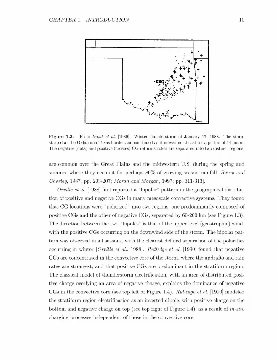
Figure 1.3: From Brook et al. [1989]. Winter thunderstorm of January 17, 1988. The stormstarted at the Oklahoma-Texas border and continued as it moved northeast for a period of 14 hours.The negative (dots) and positive (crosses) CG return strokes are separated into two distinct regions.
are common over the Great Plains and the midwestern U.S. during the spring and
summer where they account for perhaps 80% of growing season rainfall [Barry and
Chorley, 1987; pp. 203-207; Moran and Morgan, 1997; pp. 311-313].
Orville et al. [1988] first reported a “bipolar” pattern in the geographical distribu-
tion of positive and negative CGs in many mesoscale convective systems. They found
that CG locations were “polarized” into two regions, one predominantly composed of
positive CGs and the other of negative CGs, separated by 60-200 km (see Figure 1.3).
The direction between the two “bipoles” is that of the upper level (geostrophic) wind,
with the positive CGs occurring on the downwind side of the storm. The bipolar pat-
tern was observed in all seasons, with the clearest defined separation of the polarities
occurring in winter [Orville et al., 1988]. Rutledge et al. [1990] found that negative
CGs are concentrated in the convective core of the storm, where the updrafts and rain
rates are strongest, and that positive CGs are predominant in the stratiform region.
The classical model of thunderstorm electrification, with an area of distributed posi-
tive charge overlying an area of negative charge, explains the dominance of negative
CGs in the convective core (see top left of Figure 1.4). Rutledge et al. [1990] modeled
the stratiform region electrification as an inverted dipole, with positive charge on the
bottom and negative charge on top (see top right of Figure 1.4), as a result of in-situ
charging processes independent of those in the convective core.

CHAPTER 1. INTRODUCTION 11
convective core -- conventional dipole
stratiform region -- inverted dipole
positive CG with subsequent intracloud lightning
0 km
15 km
Figure 1.4: Adapted from Lyons [1996]. (Top) Schematic of the typical Great Plains mesoscaleconvective system associated with Sprites. Models of electrification are shown for the convective coreon the left and stratiform region on the right. (Bottom) Positive CG causes charge rearrangementin the cloud, which may induce subsequent intracloud “spider” discharges in the stratiform region.
Related work indicates that in the convective core, extensive vertical growth of the
thundercloud leads to the creation of a mixed-phase layer between 0C and −40C,
where graupel particles (1-10 mm snowballs) form and contribute significantly to
the charging of the thundercloud [Williams, 1995; pp. 36-38]. These “deep convective
regions” may be necessary for the formation of downwind horizontally extensive strat-
iform regions, where the highest percentage of positive CGs occur [Rutledge et al.,
1993]. Electric field soundings aboard balloons indicate that the stratiform regions of
mesoscale convective systems have multiple vertical layers of space charge, which are
nearly uniform in the horizontal dimension and each hold up to ∼1000 C of charge
[Stolzenburg et al., 1994; Marshall et al., 1996]. In light of observations of large contin-
uing currents associated with positive CGs (see Section 1.2.2), this charge structure
indicates that large reservoirs of positive charge exist in the horizontally extensive
(>100 km) stratiform regions of mesoscale convective systems. In some cases, a pos-
itive CG and continuing currents may drain charge from only part of the reservoir,

CHAPTER 1. INTRODUCTION 12
and the resulting charge rearrangement in the stratiform region may induce subse-
quent intracloud discharges, known as “spider” lightning [Williams, 1995; pp. 50-52;
Lyons, 1996] (see also Section 3.3). Sprites are associated with the occurrence of pos-
itive CGs, and most Sprites have been observed overlying the stratiform regions of
mesoscale convective systems in the mature or decaying phases (e.g., [Lyons, 1996]).
The predictions of quasi-electrostatic models of Sprite production (see Section 1.1)
are consistent with the hypothesis that large reservoirs of positive charge exist in the
stratiform regions of mesoscale convective systems.
1.3 Radio Atmospherics
In this dissertation, broadband ELF/VLF measurements of radio atmospherics are
used to assess the characteristics of individual lightning discharges from distances of
up to ∼12,000 km. Lightning radiates electromagnetic energy from a few Hz [Fuku-
nishi et al., 1997] up to many tens of MHz [Weidman and Krider, 1986]. Consistent
with the time and spatial scales of lightning discharges, the peak power radiated by
a lightning discharge is in the ELF (extremely low frequency, here 15 Hz - 1.5 kHz)
and VLF (very low frequency, here 1.5 kHz - 22 kHz) ranges [Uman, 1987; p. 118].
Radio atmospherics are the electromagnetic signals in the ELF/VLF frequency ranges
that are launched into the Earth-ionosphere waveguide by lightning discharges [Bud-
den, 1961; pp. 5,69]. Radio atmospherics are commonly called “sferics,” where the
modified spelling is used to avoid confusion with terms such as “spherical geometry.”
Sferics propagate with low but variable attenuation, typically ∼2-3 dB/1,000 km,
depending upon day/night, land/ocean and east/west propagation conditions, and
can therefore be observed at large distances (>12,000 km) from the source [Davies,
1990; pp. 367, 387-389]. The parallel-plate waveguide which guides the propagation
of sferics has as its boundaries the ground and the lower boundary of the D-region
of the ionosphere, which at VLF frequencies is ∼70 km altitude during the day and
∼80-85 km altitude at night [Thomson, 1993; Cummer, 1997].
Radio wave propagation at these frequencies is typically analyzed in terms of
waveguide modes, characterized as quasi-transverse electric and quasi-transverse mag-
netic modes in the VLF frequency range [Budden, 1962]. All of the modes except one
have cutoff frequencies at integer multiples of ∼1.8 kHz, the frequency with a free-
space wavelength equal to the twice the height of the Earth-ionosphere waveguide,

CHAPTER 1. INTRODUCTION 13
∼80-85 km at night [Cummer, 1997]. The single mode which has no cutoff frequency
and which propagates in the Earth-ionosphere waveguide at frequencies below ∼1.8
kHz is the quasi-transverse electromagnetic mode. Models of the quasi-transverse
electromagnetic mode of propagation have been used previously to obtain estimates
of the current moment of the source lightning, and to infer the magnitude of the
charge lowered from the cloud to ground [Bell et al., 1996, 1998; Cummer and Inan,
1997]. The quasi-transverse electromagnetic mode does not overlap the VLF fre-
quency range because its attenuation increases exponentially with frequency, and
most quasi-transverse electromagnetic signals are strongly attenuated above ∼1 kHz
[Greifinger and Greifinger, 1986; Sukhorukov and Stubbe, 1997].
At long ranges (e.g., 5,000-12,000 km), sferics are repeatedly observed to have an
oscillating VLF portion lasting ∼1 ms, sometimes followed by an ELF “slow tail” (e.g.,
[Hepburn, 1957; Taylor and Sao, 1970; Sukhorukov, 1992; Sukhorukov and Stubbe,
1997]). The term “slow tail” denotes its late arrival; the first maximum of the ELF
slow tail is delayed in time with respect to the VLF onset by an amount related to the
propagation distance [Wait, 1960; Sukhorukov, 1992]. This delay is a simple result of
the difference in phase velocities; the ELF slow tail propagates in the quasi-transverse
electromagnetic mode with a phase velocity of ∼0.9 c, while the VLF portion prop-
agates in the quasi-transverse electric and quasi-transverse magnetic modes with a
phase velocity much closer to c, the speed of light [Sukhorukov and Stubbe, 1997;
Cummer, 1997]. Theoretical calculations show that the ELF slow tail is excited at
significant levels only by source lightning discharges with a continuing-current com-
ponent with significant variations on the time scale of ∼1-3 ms [Wait, 1960]. In this
dissertation, we make use of this fact to deduce the strength of continuing currents
with duration ∼1-3 ms based on remote measurements of the ELF slow tails of sferics
at large source-to-receiver distances (∼12,000 km).

CHAPTER 1. INTRODUCTION 14
1.4 Contributions of this Work
The contributions of this dissertation are as follows:
• Developed novel digital signal processing techniques for automated detection
and arrival azimuth determination of radio atmospherics (“sferics”) in broad-
band ELF/VLF data on a continuous basis. Determination of the arrival az-
imuth of sferics is based on the VLF Fourier Goniometry technique [Burgess,
1993]. We demonstrated arrival azimuth measurement with ±1 precision for
sferics propagating from Nebraska to Palmer Station, Antarctica, a source-to-
receiver distance of ∼12,000 km.
• Based on ELF measurements of sferics at Palmer Station, Antarctica, demon-
strated the first evidence of continuing currents in Sprite-producing positive
CG lightning flashes. The continuing currents flow from cloud to ground for
∼1-3 ms following the positive return stroke. The radiation from these currents
enhances the ELF slow tails of sferics, which are observed at ∼12,000 km from
their source lightning.
• Based on ELF measurements of sferics at Yucca Ridge, Colorado, developed a
proxy indicator for Sprite occurrence which can estimate the number of Sprites
produced above a mesoscale convective system.
• Through measurements of ELF energy radiated from Sprites themselves, iden-
tified a quantitative relationship between the current in Sprites and total Sprite
luminosity.

Chapter 2
Broadband ELF/VLF Lightning
Detection and Location
In this chapter we describe the systems used for remote sensing of radio atmospherics
(“sferics”), the impulsive radio signals emitted by lightning discharges. We describe
the broadband ELF/VLF measurements and algorithms used for automated identifi-
cation and arrival azimuth determination of sferics. We then demonstrate the utility
and accuracy of this technique at ultra-long range (∼12,000 km) using data acquired
at Palmer Station, Antarctica.
The basic data used for measurement of radio atmospherics is broadband ELF/VLF
data recorded in digital form on magnetic tape. In some cases, the data are high-
pass filtered to avoid unwanted interference from 60 Hz ac power and its harmonics.
In other cases, the lower end of the frequency range measured extends below 60 Hz
so that the power line interference is unavoidable and must be removed in post-
processing. The sferic data analysis procedures are summarized in block diagram
form in Figure 2.1. First, interference from 60 Hz and its harmonics is removed using
a 10th-order highpass IIR Butterworth filter [Strum and Kirk, 1988; pp. 623-659]. All
filters described in this chapter use the same basic realization. The cutoff frequency
of the highpass filter is 1.5 kHz. Second, a 4 kHz bandwidth of interest is chosen to
maximize signal-to-noise ratio, as described below. Third, threshold and coherence
criteria are used to identify the time of occurrence of sferics. Fourth, the arrival
azimuths of the identified sferics are determined using the VLF Fourier Goniometry
method (see Section 2.3) [Burgess, 1993]. In the final step, the peak value of the
magnitude in both the VLF and ELF frequency bands and the average energy in
15

CHAPTER 2. ELF/VLF LIGHTNING DETECTION AND LOCATION 16
MagneticTape
Removalof 60 HzNoise
BandpassFilter
5-9 kHz
VLF FourierGoniometry
SfericMeasurement
SfericDetector
Sferictime
Arrivalazimuth
• VLF peak• ELF peak• ELF energy
Figure 2.1: ELF/VLF sferic data analysis.
the ELF band are measured and stored. These measurements result in five quanti-
ties identified for each sferic. The azimuth measurements are then triangulated with
measurements of the same sferics at other stations in order to determine lightning
location.
2.1 Broadband ELF/VLF Receiving Systems
In this section we describe the Stanford University ground-based broadband ELF/VLF
receiving systems that were used to acquire the data analyzed in this dissertation.
These systems measure electromagnetic waves in the Earth-ionosphere waveguide in
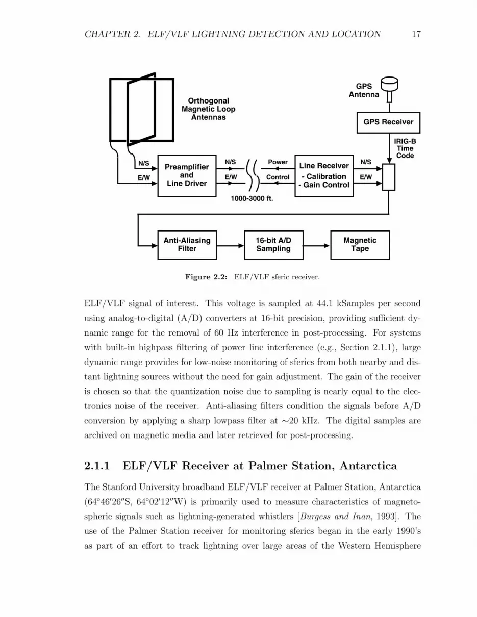
the frequency range between 15 Hz and 22 kHz. A block diagram of a broadband
receiver and recording system is shown in Figure 2.2. At each receiver location,
two orthogonal loop antennas are used to detect both components of the horizon-
tal magnetic field, normally oriented geomagnetic north-south (labelled “N/S”) and
geomagnetic east-west (labelled “E/W”). The antenna terminals are connected to a
matched preamplifier to yield flat system frequency response and maximum sensitiv-
ity for a particular antenna. The line driver-line receiver combination is used to isolate
the antennas and preamplifiers from the nearest sources of power line interference by
∼1000-3000 feet.
The output voltage of the line receiver is a scaled version of the broadband
CHAPTER 2. ELF/VLF LIGHTNING DETECTION AND LOCATION 17
IRIG-BTimeCode
GPS Receiver
GPSAntenna
N/S
E/W
OrthogonalMagnetic Loop
Antennas
MagneticTape
Anti-AliasingFilter
16-bit A/DSampling
Preamplifierand
Line Driver
N/S
E/W
Line Receiver- Calibration
- Gain Control
Power
Control
1000-3000 ft.
N/S
E/W
Figure 2.2: ELF/VLF sferic receiver.
ELF/VLF signal of interest. This voltage is sampled at 44.1 kSamples per second
using analog-to-digital (A/D) converters at 16-bit precision, providing sufficient dy-
namic range for the removal of 60 Hz interference in post-processing. For systems
with built-in highpass filtering of power line interference (e.g., Section 2.1.1), large
dynamic range provides for low-noise monitoring of sferics from both nearby and dis-
tant lightning sources without the need for gain adjustment. The gain of the receiver
is chosen so that the quantization noise due to sampling is nearly equal to the elec-
tronics noise of the receiver. Anti-aliasing filters condition the signals before A/D
conversion by applying a sharp lowpass filter at ∼20 kHz. The digital samples are
archived on magnetic media and later retrieved for post-processing.
2.1.1 ELF/VLF Receiver at Palmer Station, Antarctica
The Stanford University broadband ELF/VLF receiver at Palmer Station, Antarctica
(6446′26′′S, 6402′12′′W) is primarily used to measure characteristics of magneto-
spheric signals such as lightning-generated whistlers [Burgess and Inan, 1993]. The
use of the Palmer Station receiver for monitoring sferics began in the early 1990’s
as part of an effort to track lightning over large areas of the Western Hemisphere

CHAPTER 2. ELF/VLF LIGHTNING DETECTION AND LOCATION 18
2 103 104
-6
-4
-2
0
2
4
Frequency (Hz)
Sys
tem
res
po
nse
(d
B)
10-8
Figure 2.3: Palmer Station ELF/VLF receiver frequency response.
[Hakeman et al., 1993].
Calibration of the ELF/VLF receiver is performed to determine the conversion
factor between the output voltage and the equivalent magnetic field of a wave incident
on the loop antenna and to measure the system frequency response [Paschal, 1988]. To
perform the calibration procedure, one injects a sinusoidal current of known amplitude
at the antenna terminals and measures the output with a true-rms digital multimeter.
During this measurement, each loop antenna is disconnected in turn and replaced by
a “dummy loop” that has inductance and dc resistance equivalent to that of the loop
antenna. This method was used to obtain the system frequency response for the
Palmer Station ELF/VLF receiver, shown in Figure 2.3. At the lower frequencies,
the Palmer response is flat within ±1 dB down to 1 kHz, then it decays at ∼10
dB/decade, with a -3 dB point at ∼300 Hz. At higher frequencies the system response
is flat within ±1 dB until the frequency exceeds the ∼20 kHz cutoff frequency of the
lowpass anti-aliasing filters.
At Palmer the data are sampled using a Sony PCM 601-ESD encoder, which
samples two analog audio input signals continuously and encodes the resulting digital

CHAPTER 2. ELF/VLF LIGHTNING DETECTION AND LOCATION 19
data onto one output video signal using pulse code modulation. Upon playback, the
pulse code modulation decoder allows error-free recovery of the two streams of digital
samples at 44.1 kSamples per second. A video cassette recorder is used to write
the video signal onto magnetic tape. The audio input of the same recorder allows
simultaneous recording of an IRIG-B timing signal [Burgess, 1993]. IRIG-B is a 1-ms
resolution time encoding standard, which in this work is derived from signals received
by GPS or GOES receivers, which are both synchronized to coordinated universal
time by the National Institute of Standards and Technology, formerly the National
Bureau of Standards.
2.1.2 ELF/VLF Sferic Receiver at Yucca Ridge, Colorado
A new ELF/VLF Sferic Receiver was designed and built at Stanford University and
installed at Yucca Ridge Field Station (4040′06′′N, 10456′24′′W), 15 km northeast of
Fort Collins, Colorado, during July 1996. The sensitivity of the antenna-preamplifier
combination is ten times lower than the Palmer system to avoid saturation of the
preamplifier due to strong sferics from nearby (∼500 km or nearer) lightning. The
motivation for the design of a new system was to extend the low end of the frequency
response further into the ELF band to enable accurate measurement of electromag-
netic radiation produced by lightning continuing currents (see Section 1.2.2) on time
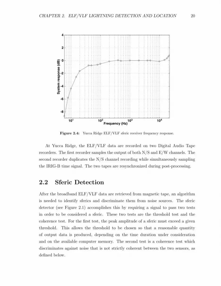
scales longer than ∼3 ms. The Yucca Ridge system frequency response is flat to ±1
dB down to ∼30 Hz, with a -3 dB point of ∼15 Hz, as shown in Figure 2.4. Table
2.1 compares the characteristics of the Palmer and Yucca Ridge systems.
Table 2.1: Comparison of Palmer and Yucca Ridge broadband systems
Parameter PA system YR systemShape triangle square
Length of sides 9 x 18 m 81 x 81 cmNumber of turns 1 146
Wire gauge # 6 # 18Resistance 61.5 mΩ 10ΩInductance 65 µH 60 mH
Cutoff frequency ∼300 Hz ∼15 Hz
CHAPTER 2. ELF/VLF LIGHTNING DETECTION AND LOCATION 20
1 2 3 410 10 10 10
-8
-6
-4
-2
0
2
4
Frequency (Hz)
Sys
tem
res
po
nse
(d
B)
Figure 2.4: Yucca Ridge ELF/VLF sferic receiver frequency response.
At Yucca Ridge, the ELF/VLF data are recorded on two Digital Audio Tape
recorders. The first recorder samples the output of both N/S and E/W channels. The
second recorder duplicates the N/S channel recording while simultaneously sampling
the IRIG-B time signal. The two tapes are resynchronized during post-processing.
2.2 Sferic Detection
After the broadband ELF/VLF data are retrieved from magnetic tape, an algorithm
is needed to identify sferics and discriminate them from noise sources. The sferic
detector (see Figure 2.1) accomplishes this by requiring a signal to pass two tests
in order to be considered a sferic. These two tests are the threshold test and the
coherence test. For the first test, the peak amplitude of a sferic must exceed a given
threshold. This allows the threshold to be chosen so that a reasonable quantity
of output data is produced, depending on the time duration under consideration
and on the available computer memory. The second test is a coherence test which
discriminates against noise that is not strictly coherent between the two sensors, as
defined below.

CHAPTER 2. ELF/VLF LIGHTNING DETECTION AND LOCATION 21
Whistlers
Sferics
Omega signals
Figure 2.5: Spectrogram of broadband data from Palmer Station, Antarctica.
For automated detection of sferics in broadband ELF/VLF data, it is necessary to
take into account the characteristics and variability of other electromagnetic signals
in the same frequency range. Figure 2.5 is a spectrogram from 100 Hz to 16 kHz
of five seconds of broadband data recorded at Palmer Station, Antarctica, during
typical summer nighttime conditions. The vertical lines are sferics, which are broad
in frequency and short in duration. They exceed the minimum amplitude in the
spectrogram above ∼5-7 kHz, and the ELF component of some sferics is clearly vis-
ible below ∼500 Hz. The horizontal segments of approximately one-second duration
with frequency between 10 and 14 kHz are the Omega navigation transmitter signals
[Burgess, 1993]. The single horizontal line at 10 kHz is a locally injected amplitude-
modulated clock signal for redundancy in timing. Finally, the gently curving lines
in the lower right corner are whistlers, the component of lightning energy which has
propagated within the density inhomogeneities called “ducts” in the earth’s magne-
tosphere and is received on the ground [Helliwell, 1965]. Their “whistling” quality is

CHAPTER 2. ELF/VLF LIGHTNING DETECTION AND LOCATION 22
due to dispersion experienced in propagation through the cold plasma in the magne-
tosphere [Davies, 1990; pp. 368-370]. If one wishes to detect only sferics, whistlers
constitute a naturally-generated “noise source.”
In the frequency band between 5 and 9 kHz there is strong sferic energy and little
interference from natural or anthropogenic sources (see Figure 2.5). We implement
the threshold test, which is the first of the two tests, in this frequency band. For
the threshold test, we load a two-second block of data into memory, use a bandpass
filter to eliminate all but the 5 to 9 kHz band, compute the total magnetic field and
detect peaks exceeding a selectable threshold. Explicitly, where BNS represents the
measured N/S component of wave magnetic field and BEW represents the measured
E/W component of the wave magnetic field, we find the magnitude of the incident
wave magnetic field as B =√
BNS2 + BEW
2. Maxima in B which exceed the given
threshold are recorded as possible sferic occurrences. This test is performed in two-
second blocks for the entire data set under analysis.
To verify sferic occurrence, the possible sferic data sets are also subjected to
the coherence test to discriminate between sferics and random noise sources. This
coherence test requires the signals on each antenna to be in phase or 180 degrees
out of phase. To implement the coherence test, for each of BNS(t) and BEW(t), we
take the Fast Fourier Transform (FFT) of 4 ms of data using a Hamming window
[Oppenheim and Schafer, 1989; p. 447], and save the 17 frequency domain samples in
the 5 to 9 kHz frequency band. The coherence test compares the phases of BNS(f)
and BEW(f) and finds the number of the frequency domain samples having phase
coherence. A sample i is said to have phase coherence if either
| BNS(fi) − BEW(fi)| < ε, or
| BNS(fi) − BEW(fi)| − 180 < ε
is true. We use ε ∼ 5, and a sferic passes the coherence test if at least a fixed per-
centage of the frequency domain samples between 5 and 9 kHz have phase coherence.
The fixed percentage is chosen to be 35% based on the particular features of sferics
and of the ambient noise background.
Each waveform that passes both the threshold and the coherence tests is identified
as a sferic. The time of the sferic is recorded with ∼1 ms precision.

CHAPTER 2. ELF/VLF LIGHTNING DETECTION AND LOCATION 23
2.3 Sferic Arrival Azimuth Determination
After identification of each sferic, we need to determine the location of its source
lightning discharge. This section describes arrival azimuth determination at a single
receiving station. In order to determine the actual location of a lightning flash, one
needs to perform triangulation of measurements at multiple locations. Triangulation
algorithms are readily available [Orville Jr., 1986], therefore in this dissertation we
address the method and results of arrival azimuth determination at a single receiving
station.
VLF Fourier Goniometry is a VLF direction-finding method using two orthogonal
magnetic loop antennas to find the major axis of the polarization ellipse of the in-
coming wave [Burgess, 1993; Inan et al., 1996b; Reising et al., 1996]. Burgess [1993]
verified the accuracy of VLF Fourier Goniometry by comparing the measured arrival
azimuths of signals from eight Omega navigation transmitters to their expected ar-
rival azimuths at Palmer Station, Antarctica. He found agreement between expected
and actual bearings of ±5 and applied VLF Fourier Goniometry to direction find-
ing on whistlers. In this section we apply the same method to determine the arrival
azimuth of sferics at Palmer Station. This implementation assumes that the sources
of the waves are on or near the ground so that the elevation angle of arrival at the
receiver (>1000 km away) is nearly zero [Cousins, 1972].
VLF Fourier Goniometry uses the Fourier Transform to synthesize a rotating
antenna, or goniometer, over a range of frequencies in the band of interest. A wave
with time dependence cos(2πf0t) incident on a goniometer rotating at a frequency
f0 produces a phase-shifted output dependent upon the direction of arrival. For a
zero phase reference corresponding to the goniometer pointing north, the phase shift
of the output is equivalent to the bearing of the incoming signal. To implement the
same goniometer at frequency f0 with two fixed orthogonal antennas, we synthesize a
Fourier Goniometer signal BFG using the outputs of the two antennas, BNS and BEW,
as
BFG(f0) =1
τ
∫ τ
0[BNS cos(2πf0t) + BEW sin(2πf0t)]dt
The integral averages the signal over the duration of the sferic, τ . For a general
frequency f , we have,
BFG(f) =1
τ
∫ τ
0(BNS − jBEW) e j2πftdt

CHAPTER 2. ELF/VLF LIGHTNING DETECTION AND LOCATION 24
Hence BFG(f) is the Fourier transform of the complex quantity which has real part
BNS and imaginary part −BEW. The phase of this complex quantity is the bearing
of the received signal, and its magnitude is the magnitude of the total magnetic field,
B.
For computational efficiency the Fourier Goniometer signal, BFG(f), is computed
using the Fast Fourier Transform algorithm. We use N samples in the frequency
domain for 5 kHz < fi < 9 kHz. In this case we use the same frequency range for
sferic detection (see Section 2.2) and arrival azimuth determination. Since the Omega
navigation transmitters were decommissioned during 1997, the 10-14 kHz frequency
range may be more useful for arrival azimuth determination in future work. The
arrival bearing of each sferic is estimated by averaging the arrival direction in each
frequency bin, using the magnitude in that bin as a weighting function. Expressing
the arrival azimuth of a sferic as Φ, we have,
Φ =
N−1∑i=0
|BFG(fi)| BFG(fi)
NN−1∑i=0
|BFG(fi)|
.
With two orthogonal magnetic loop antennas, if a signal is deduced to arrive
at a certain bearing, it is not possible to determine if it actually arrived from this
bearing or from Φ±180 . Therefore, we have a 180 ambiguity in arrival azimuth
determination. In practice, since VLF propagation over ice is highly lossy [Rogers
and Peden, 1975], nearly all sferics measured at Palmer Station, Antarctica, arrive
from bearings between -90 and +90 (see Figure 2.6). Therefore, the arrival azimuth
of each sferic observed at Palmer is recorded in the domain [−90, +90], along with
its time of occurrence and total magnitude.
2.4 Precision of Sferic Arrival Azimuth
Determination
Analysis of broadband VLF measurements at Palmer Station, Antarctica, as de-
scribed in Sections 2.2 and 2.3, allows detection of sferics from lightning at least as

CHAPTER 2. ELF/VLF LIGHTNING DETECTION AND LOCATION 25
-40˚ -30˚ -20˚ -10˚ 0˚
IntenseMidwestern
Thunderstorm
Direction-findingfrom Palmer Station,
Antarctica
Propagation Pathsto Palmer from N. Hemisphere
~12,000 km
Figure 2.6: View of great circle propagation paths from North America to Palmer Station,Antarctica.

CHAPTER 2. ELF/VLF LIGHTNING DETECTION AND LOCATION 26
Storm B
Storm C
YR
Storm A
-30˚ -20˚
Bearings from PA-40˚
30˚ N
45˚ N
120˚ W
90˚ W
Figure 2.7: Thunderstorm activity from 0644 to 0800 UT on August 1, 1996. Pluses show locationsof positive cloud-to-ground flashes observed by the NLDN with peak current exceeding 23 kA. TheYucca Ridge Field Station in Colorado is denoted by “YR.”
far as the Great Plains, at a range of ∼12,000 km from Palmer (see Figure 2.6). In
order to determine the precision of the arrival azimuth determination method pre-
sented in Section 2.3, we compare the measured arrival azimuth, Φ, of individual
sferics with the expected arrival azimuth derived from the known locations of their
source lightning discharges. Since those locations of CG discharges in the continental
U.S. are measured to ∼0.5 km precision by the NLDN (see Section 1.2.4), we choose
thunderstorms in the continental U.S. to verify the precision of sferic arrival azimuth
determination.
Several storms occurring on August 1, 1996, were studied using lightning location
CHAPTER 2. ELF/VLF LIGHTNING DETECTION AND LOCATION 27
Pea
k cu
rren
t (k
A)
0729:00 0729:01 0729:02 0729:03 0729:04 UT
-40
0
40
80
120
NLDN 01 Aug 96 (Continental U. S. coverage only)
C1 C2 C3B1
B2
A1
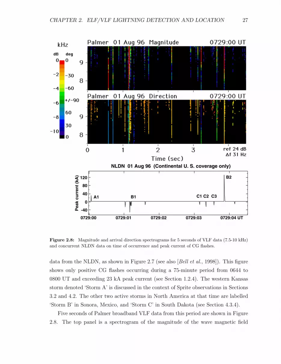
Figure 2.8: Magnitude and arrival direction spectrograms for 5 seconds of VLF data (7.5-10 kHz)and concurrent NLDN data on time of occurrence and peak current of CG flashes.
data from the NLDN, as shown in Figure 2.7 (see also [Bell et al., 1998]). This figure
shows only positive CG flashes occurring during a 75-minute period from 0644 to
0800 UT and exceeding 23 kA peak current (see Section 1.2.4). The western Kansas
storm denoted ‘Storm A’ is discussed in the context of Sprite observations in Sections
3.2 and 4.2. The other two active storms in North America at that time are labelled
‘Storm B’ in Sonora, Mexico, and ‘Storm C’ in South Dakota (see Section 4.3.4).
Five seconds of Palmer broadband VLF data from this period are shown in Figure
2.8. The top panel is a spectrogram of the magnitude of the wave magnetic field

CHAPTER 2. ELF/VLF LIGHTNING DETECTION AND LOCATION 28
2040
6080100
-80 -60 -40 -20 0 20 40 60 80
0
100
200
300
Arrival Azimuth (deg)VLF peak (pT)
Nu
mb
er o
f S
feri
cs
Figure 2.9: Histogram of the number of sferics as a function of both the peak value of the VLFmagnetic field intensity and the arrival azimuth (see Figure 2.6). The observation period was from0715 to 0730 UT on August 1, 1996.
measured in the 7.5 to 10 kHz band. The magnitude scale is shown in dB on the left
side of the color bar. The middle panel is a spectrogram of the direction of arrival
in the same frequency range. The arrival bearing is given rotating from 0 north as
red, to the west as green, then from the east equivalently as green, and back to the
north as purple. All azimuth values are given in the domain [−90, +90], due to
the 180 ambiguity (see Section 2.3). The bottom panel shows the peak current of
CG lightning flashes observed by the NLDN during the same time period. The sferic
labelled A1 arrives at Palmer from Storm A at -29 bearing, in agreement with its
orange color in the direction spectrogram. Similarly, sferic B2 arrives at Palmer from
Storm B at -40 bearing, and has a yellow-orange color in the direction spectrogram.
All sferics detected within a 15-minute interval are shown in Figure 2.9 as a his-
togram of the number of sferics versus both the magnitude of the sferic (given as peak
value of the VLF magnitude) and the arrival azimuth at Palmer. Storm B is clearly
visible from -41 to -38 bearing, and Storms A and C combine to form the highest
peak, between -31 and -25 bearing.
To determine the precision of sferic arrival azimuth determination, lightning lo-
cations measured by NLDN with ∼0.5 km precision were compared to the bearings
measured at Palmer. Using the NLDN locations as the source, and assuming that
most of the sferic energy propagated directly along the great circle path from the
lightning discharge to the receiver at Palmer, the difference between the expected
and measured arrival azimuths was determined for each of 328 flashes. The resulting

CHAPTER 2. ELF/VLF LIGHTNING DETECTION AND LOCATION 29
-4 -3 -2 -1 0 1 2 3 40
10
20
30
40
50
60
70
80
90
100
Arrival azimuth error (deg)
Palmer Station 12 July 94 0510-0712 UT
Nu
mb
er o
f sf
eric
s
Figure 2.10: Arrival azimuth error of 328 sferics received at Palmer Station, Antarctica, fromsource lightning in Nebraska, a source-to-receiver distance of ∼12,000 km.
statistics are shown as a histogram of number of sferics as a function of arrival az-
imuth error in Figure 2.10. Over 90% of the sferics have a bearing error of ±1 or less.
At a range of ∼12,000 km, ±1 bearing error corresponds to ±200 km in transverse
distance error.
In this chapter we have described the receiving systems and algorithms used for
broadband ELF/VLF remote sensing of sferics originating in lightning. Using a single
broadband ELF/VLF receiving station, this technique identifies lightning flashes at a
source-to-receiver distance of at least ∼12,000 km and measures arrival azimuth with
an accuracy of ±1 .

Chapter 3
Association of Sprites and
Cloud-to-Ground Lightning
This chapter describes the temporal association of visually observed Sprites in the
mesosphere and lower ionosphere with cloud-to-ground lightning in the troposphere.
The association of Sprites with positive CG lightning has been reported previously
[Boccippio et al., 1995; Winckler et al., 1996; Reising et al., 1996; Lyons, 1996]. This
study extends previous work by analyzing a large number of Sprites and by measuring
the delay between a positive CG return stroke and the occurrence of a Sprite with
high time resolution (∼17 ms).
3.1 Identification of Sprite Onset Time
We rely exclusively on ground-based observations of Sprites, which have the advantage
of recording all Sprites above a thunderstorm on a continuous basis. In this context,
“all Sprites” means those Sprites which are in the field of view and are detectable
above the noise level of the intensified charge-coupled device (CCD) camera. For the
ground-based observations, we use an image-intensified black-and-white Pulnix CCD
camera with a ∼19 wide by ∼14 high field of view. In order to be detected, a
Sprite must emit enough photons to exceed noise generated in the imaging system
and recorded on the videotape. This noise appears to the observer as “speckle” on
the video screen. Weak Sprites are best detected by watching a video in motion,
as opposed to single images, because the human eye is more sensitive to temporal
changes than to stationary pattern differences.
30

CHAPTER 3. ASSOCIATION OF SPRITES AND CG LIGHTNING 31
-33 -17 0 17 33 50 67 84 100Time (ms)
Frame 1: labelled 33 ms
Frame 2: labelled 67 ms
Sprite Onset in Same Frame in Backup:
Sprite Onset in Previous Framein Backup:
50-67 ms
33-50 ms
1A
1B
1A
1B
2A
2B
2A
2B
Figure 3.1: Determination of time of Sprite onset to 16.7 ms precision (see text for detail).
Current video hardware is still based on a variation of the RS-170 video standard
adopted by the broadcast industry in 1957. RS-170 is a 30 frames per second, 2:1
interlaced format that accomplished flicker-free video within a broadcast bandwidth
that could be transmitted in the 1950s [Burke, 1996; p. 736]. Interlacing is accom-
plished by reading first the odd horizontal scan lines, or “first field,” and then the
even scan lines, or “second field.” In the normal frame-integration mode, the first
and second fields each last 1/30 sec (33 ms), but they are offset in time from each
other by 1/60 sec (16.7 ms) [Burke, 1996; p. 775]. As shown in Figure 3.1, field 1A is
sensitive to illumination from t =0 to 33.3 ms, and field 1B is active from t =16.7 to
50 ms. Frame 2 begins at t =33.3 ms, giving a video rate of 30 frames/sec.
For Sprite monitoring, the intensified CCD camera signal is recorded on a standard
VHS video cassette recorder (VCR). A TrueTime video time inserter card writes the
time across the bottom of the video frame with 1-ms resolution, as shown in Figure
1.1. The time stamp is delayed by 33 ms from the beginning of the frame, so that if
a frame starts at the beginning of second S, the time stamp reads S.033. The video
inserter card derives its time from a GPS clock with time referenced to universal

CHAPTER 3. ASSOCIATION OF SPRITES AND CG LIGHTNING 32
coordinated time to better than 200 ns.
Since the vertical extent of Sprite images is greater than one horizontal scan
line, individual fields can be used to find the onset time of Sprite luminosity with
a time resolution of 16.7 ms. A single field of each frame is viewed using the pause
function on a standard VCR. In order to view the other field of each frame, the
videotape was played on one VCR, and the output was recorded on a second VCR
from a different manufacturer. The resulting backup videotape, when viewed using
the pause function, displayed a different field of each frame, compared to the original
videotape. We can therefore view each field independently using both the original
and backup videotapes.
We illustrate the determination of Sprite onset time to 16.7 ms resolution in Figure
3.1, where two consecutive frames are labelled 1 and 2, while the first and second fields
within each frame are labelled A and B, respectively. The horizontal axis gives the
time relative to the beginning of frame 1, and the time stamp shown on each frame is
33 ms after the beginning of exposure of its first field. When using the pause function,
we view field A on the original tape and field B on the backup tape. Referring to
Figure 3.1, if the Sprite onset is observed on the same frame (here frame 2) on both
the original and the backup, the Sprite onset is during the second half of field 2A
or, equivalently, the first half of field 2B. If the Sprite onset is observed on frame 2
of the original tape and frame 1 of the backup tape, then the Sprite onset is during
the second half of field 1B or, equivalently, the first half of field 2A. This method
enables the determination of the onset time of any observed Sprite with a precision
of ∼17 ms.
3.2 Association of Sprites and Positive
Cloud-to-Ground Flashes
In order to determine the association of Sprites and cloud-to-ground (CG) flashes,
the time of Sprite onset can be compared to the onset time of sferics recorded at the
same location. The VLF sferics reported here are those sferics which are generated by
CG lightning flashes. VLF sferics propagate at a phase velocity nearly equal to c, the
speed of light [Cummer, 1997]. Since both the VLF sferic and the visible light of the
Sprite travel nearly the same distance at nearly the same propagation speed (c), the

CHAPTER 3. ASSOCIATION OF SPRITES AND CG LIGHTNING 33
relative times of their occurrence can be considered equal to the relative times of their
arrival at the receiving location, within an error of <0.1 ms. As a result, measurement
of the time between sferic onset and Sprite onset yields the delay between a CG flash
and a subsequent Sprite.
To illustrate the association between Sprites and positive CG flashes, we report
results of observations of Sprites above a mesoscale convective system in western
Kansas on August 1, 1996 (see Figure 3.2). Continuous video observations of Sprites
were conducted at Yucca Ridge (see Section 2.1.2) as part of the Stanford / Lock-
heed Fly’s Eye experiment [Inan et al., 1997]. Simultaneously, the signals from two
orthogonal magnetic loop antennas oriented geographic N/S and E/W were recorded
digitally on a continuous basis (see Section 2.1).
During the August 1 observations, the intensified CCD camera was pointed south-
east, with a field of view bounded by the segments shown in Figure 3.2. The NLDN-
recorded flash locations are denoted by dots for negative CG flashes and by pluses
for positive CG flashes. The color code indicates the strength of the flash in terms of
NLDN-measured peak current, and the red circles indicate the locations of positive
CGs which are associated with Sprites. The CG lightning polarity exhibits the ex-
pected “bipolar” pattern for a mesoscale convective system, as described in Section
1.2.5. The convective core of the storm is to the southwest, where negative CGs are
concentrated, and the downwind stratiform region is to the northeast, where most
positive CGs occurred [Orville et al., 1988; Rutledge et al., 1990]. All Sprites were
observed over the trailing stratiform precipitation region of the mesoscale convective
system, consistent with previous observations [Sentman et al., 1995; Winckler et al.,
1996; Lyons, 1996]. Previous studies have shown that the center of the Sprite may be
displaced from the NLDN-detected CG location by as much as ∼40 km [Winckler et
al., 1996; Lyons, 1996], which explains the observation of one Sprite associated with
a CG location just outside (north of) the camera field of view (see Figure 3.2).
During the period 0644-0907 UT, or 1:44 to 4:07 a.m. local (CDT) time, the
intensified CCD camera observed 98 Sprites above the mesoscale convective system
in western Kansas, giving an average occurrence rate of one Sprite every ∼90 seconds.
A three-minute period from ∼0815-0818 UT was eliminated from the analysis because
no video data were available. During the 139-minute observation period, there were
∼9400 CGs recorded by NLDN above a peak current threshold of 10 kA, and 12% of
these CG flashes were of positive polarity.

CHAPTER 3. ASSOCIATION OF SPRITES AND CG LIGHTNING 34
Lat
itu
de
(deg
)
Longitude (deg)
YR *
Sprites
10-26 kA > 26 kA> 26 kA
10-26 kA
positive CGs negative CGs
~ 500 kmdistance
-105 -104 -103 -102 -101 -100 -99 -9836
37
38
39
40
41
* YR = Yucca Ridge
9398 flashes, 12% positive91 sprite-associated +CGs
01 Aug 96 0644-0907 UT
Figure 3.2: NLDN lightning locations and camera field of view for observations from Yucca Ridge,Colorado on August 1, 1996.
The onset times of all 98 Sprites were compared to occurrence times of sferics
and NLDN-recorded CG flashes. In 94 (96%) of the cases, the Sprite was associated
with a positive CG. Of these 94, 85 of the Sprite onset times were within 200 ms
after the occurrence of the positive CG. Four of the other Sprites occurred 200-400
ms after the positive CG. In each of three other cases, two Sprites were observed
within ∼200-300 ms following a single positive CG. For two of the 94, the NLDN
did not detect the CG, but a sferic of positive polarity and CG characteristics [Inan
et al., 1996b] was observed in association with the Sprite. In the remaining four
of 98 Sprites, the association is unclear because no positive CGs occurred for at
least 1 second before the Sprite onset. However, after the Sprite appeared there
was a subsequent positive CG, within 150-300 ms in three of the four cases, and
∼700 ms later in the fourth case. The association of the Sprites and the subsequent
positive CGs is unclear; yet the process that triggered the Sprite may be part of an

CHAPTER 3. ASSOCIATION OF SPRITES AND CG LIGHTNING 35
extensive intracloud process (“spider” lightning) that can last as long as ∼600 ms and
may be connected to the subsequent occurrence of positive cloud-to-ground lightning
(see Figure 1.4) [Williams, 1995, pp. 50-52; Lyons, 1996]. It is known that the
stratiform precipitation region of large mesoscale convective systems is favorable to
horizontally extensive regions of positive charge generation and leads to large positive
CGs [Rutledge et al., 1993]. Our understanding of these events is limited by a lack
of data, but the Lightning Detection and Ranging system at Kennedy Space Center
is capable of three-dimensional mapping of intracloud processes and is being used to
investigate horizontally extensive intracloud and CG processes [Stanley et al., 1997].
All Sprite onset times were checked for possible association with negative CGs.
Negative CGs were recorded by NLDN within ∼400 ms of nearly half of the Sprite
onsets. However, in all except two cases, a stronger association of the Sprite with the
positive CG than with the negative CG is demonstrated by one of the following: (1)
the negative CG is out of the camera field of view, (2) the positive CG is closer in
time to the Sprite onset than the negative CG, or (3) the positive CG occurs before
the Sprite and the negative CG occurs afterward. In the first of the two cases where
a negative CG is closer in time to the Sprite onset than any NLDN-recorded positive
CG, there is a positive CG not detected by the NLDN but detected by identification
of a sferic at that time with positive CG characteristics. Sferics generated by CGs
have characteristics which distinguish them from other sferics produced by intracloud
lightning, and the polarity of a sferic can be uniquely identified [Inan et al., 1996b].
The positive CG identified by a sferic is closer in time to Sprite onset than the negative
CG. In the second exceptional case, the positive CG occurs ∼150 ms before the Sprite
onset and the negative CG occurs ∼60 ms before the Sprite onset, indicating a more
likely temporal association between the negative CG and the Sprite.
In summary, for the 139 minutes of observation on August 1, 1996, in 96% of
the cases a positive CG occurs before Sprite onset, usually within ∼200 ms. In the
remaining 4% of cases, a positive CG follows Sprite onset, and may be involved in an
interconnected intracloud process (“spider” lightning) triggering both the Sprite and
the positive CG. There was only one case out of 98 in which a Sprite was temporally
associated more closely with a negative CG than any positive CG.
These results are consistent with previous work. Two midwestern mesoscale con-
vective systems were studied using video observations of Sprites at Yucca Ridge and
sferics measurements at Palmer Station, Antarctica [Reising et al., 1996] (see also

CHAPTER 3. ASSOCIATION OF SPRITES AND CG LIGHTNING 36
Sections 4.3.2 and 4.3.3). During 122 minutes of observation on July 12, 1994, 44
Sprites were observed, and sferics of positive CG polarity were observed at Palmer
Station in association with 95% of the Sprites. The NLDN recorded positive CGs
within ±100 ms of the Sprite event in only 70% of the cases; however, upgrade of
the NLDN upgrades to the Improved Accuracy from Combined Technology between
1994 and 1995 improved its detection efficiency for complex events (see Section 1.2.4)
[Cummins et al., 1998; Idone et al., 1998b]. On July 15, 1995, 35 Sprite events were
observed in 104 minutes, and sferics of positive CG polarity were measured at Palmer
Station in association with 97% of the Sprites. The NLDN recorded positive CG
flashes in 83% of the cases, showing the improvement due to the NLDN upgrade.
Similarly, Boccippio et al. [1995] reported positive CGs recorded by NLDN in associ-
ation with 86% and 82% of Sprites, for mesoscale convective systems on July 12, 1994,
and September 7, 1994, respectively. Lyons [1996] reports that 94% of 36 Sprites ob-
served during a 4.5 hour period on August 6, 1994, were temporally associated with
positive CGs recorded by the NLDN.
3.3 Delays between Positive CG Flashes and Sprite
Onsets
A subset consisting of 17 of the 98 Sprites observed on August 1, 1998, and occurring
from 0817 to 0832 UT, were analyzed by Bell et al. [1996; 1998]. In Figure 3.3 we
illustrate the broad range of delays between the positive CG and the onset of each
Sprite. For 17 Sprites observed by the intensified CCD camera during the 15 minute
period, the delays ranged from ∼1 ms to ∼110 ms. The Bell et al. [1998] study also
used the ELF portion of sferics observed at Yucca Ridge to determine the magnitude
of the continuing currents (see Section 1.2.2) that followed the first return strokes of
these positive CG discharges. This task was accomplished by using a well established
model of ELF wave propagation in the Earth-ionosphere waveguide [Greifinger and
Greifinger, 1986; Sukhorukov, 1992].
The total charge removed from the cloud to the ground can be derived from the
time-integral of the current waveform, denoted by the following expression:
QT =∫ τ
oI(t)dt

CHAPTER 3. ASSOCIATION OF SPRITES AND CG LIGHTNING 37
0 2 4 6 8 10 12 14 16
0
30
60
90
120
32
53
38
20
38
23
10
6034
100
110 27
27
45112
23
54
Event No.
CG
to
Op
tica
l Sp
rite
Del
ay (
ms)
Video field duration (16.7 ms)
Charge loweredto ground (C)
Figure 3.3: From [Bell et al., 1998]. Time delay between the causative positive CG discharge(t = 0) and the video field in which the Sprite first appeared, for each of the 17 events. The timeduration of the video field is indicated by two dark circles connected by a vertical line. The numberimmediately above each video field marker represents the positive charge (QT ) lowered to groundduring the intense continuing currents that followed the first positive return stroke, assuming l = 10km.
where the discharge begins at t = 0 and τ represents the time at which the measured
sferic falls below the RMS noise level. The charge lowered to ground, assuming a
cloud-to-ground distance of l = 10 km, is given by the number above each segment
in Figure 3.3, from Bell et al. [1998]. Most of these 17 events exhibit delays of <30
ms between the positive CG and subsequent Sprite. The average value of QT for
the eight discharges that occurred within 15 ms of the beginning of the video field
is QT ∼ 65C, while for the others, QT ∼ 30C, and the average time delay until the
beginning of the video field was ∼55 ms. These observations indicate that there may
be at least two ways by which a Sprite is produced. The first mechanism requires the
transfer of a large amount (∼100 C) of positive charge from a thundercloud during a
positive CG return stroke and subsequent continuing current, in which case a Sprite
is produced shortly thereafter. This mode applies to events 7, 9, and 15 in Figure 3.3.
Alternatively, a positive CG which transfers a smaller amount of charge (∼10-50 C)

CHAPTER 3. ASSOCIATION OF SPRITES AND CG LIGHTNING 38
from the cloud to the ground may induce subsequent intracloud “spider” lightning
discharges in nearby regions of the cloud (see Figure 1.4). These intracloud discharges
may lead to Sprite production, where the Sprite appears >40 ms after the positive
CG. This mode applies to events 1, 2, 3, 8, 13, and 17 in Figure 3.3. An example of
connected positive CG and intracloud “spider” discharges is shown schematically in
Figure 1.4 (see also Figure 1 of Marshall et al. [1996]).
The following chapter addresses the question of which positive CGs lead to Sprites
by developing a proxy measure for Sprite occurrence based solely on broadband
ELF/VLF measurements of the sferic launched by each positive CG.

Chapter 4
ELF Sferic Energy as a Proxy
Indicator for Sprite Occurrence
As was discussed in Section 3.2, Sprite occurrence is nearly always associated with a
positive cloud-to-ground flash (CG). However, on average only ∼15-20% of positive
CGs during the Sprite-producing phase of mesoscale convective systems are associ-
ated with Sprite occurrence [Reising et al., 1996; Lyons, 1996]. The assessment of the
salient characteristics of those CG flashes which lead to Sprite production is therefore
an outstanding question, which we address in this chapter. There are many charac-
teristics of CG discharges which may be important for Sprite production, including
the amount of charge removed from the cloud, the strength of the discharge as mea-
sured by radiated sferic intensity, and the altitude and lateral extent of the active
thundercloud. The most readily accessible parameter is the peak lightning current as
measured by the NLDN; however, the NLDN-recorded peak current has been shown
not to be a good indicator of the Sprite-producing capacity of a positive CG (see
Section 4.2 and Reising et al. [1996]).
Video observations are often limited by foreground clouds which obscure the ob-
server’s view of the area of the sky where Sprites occur. For example, at Yucca Ridge
during summer 1996 (see Section 2.1.2), clouds reduced visibility of the area of the sky
where Sprites were expected to occur on >40% of possible evenings of observation.
In addition, video observations are limited to line-of-sight visibility and to ∼1000 km
range from the observation camera [Lyons, 1996]. In order to determine the total rate
of Sprite occurrence on continental and global scales, as well as the characteristics of
storms which lead to Sprite production, one needs a proxy for Sprite occurrence that
39

CHAPTER 4. PROXY INDICATOR FOR SPRITE OCCURRENCE 40
is based on remote measurements and is independent of direct video observations.
This chapter describes a proxy for Sprite occurrence based on individual CG flashes
using sferics measurements at both medium range (∼600 km) and at ultra-long range
(∼12,000 km) from the source lightning.
Other techniques have been explored as possible indicators of Sprite occurrence,
including excitation of the resonances of the Earth-ionosphere cavity (also known
as “Schumann resonances”) [Boccippio et al., 1995; Fullekrug and Reising, 1997].
Boccippio et al. [1995] reported that 95% and 78% of Sprites were accompanied by
ELF transients in the Schumann resonance frequency range in the storms studied
on July 12, 1994, and September 7, 1994, respectively (see Section 4.3.2). In order
to use ELF transient events as a proxy indicator for Sprite occurrence, one would
also need to know the number of ELF transients which were not accompanied by
Sprites. The only information that the authors provide in this context is that the
interval between successive transients was several seconds and that a total of 97 Sprites
were observed over a combined study duration of ∼7 hours, indicating that many
other ELF transients exceeded their detection threshold. Fullekrug and Reising [1997]
found that in a 97-minute period, 30 discrete excitations of the Earth-ionosphere
cavity resonances associated with CG flashes in a Kansas Sprite-producing storm
were simultaneously detected in Hollister, California, and in Silberborn, Germany. A
full 80% of these 30 Earth-ionosphere cavity resonance events were associated with
Sprite-producing positive CG flashes, suggesting the possibility of using ultra-long
range Earth-ionosphere cavity resonance event detection as a proxy for Sprites.
In this chapter we describe a proxy indicator for Sprite occurrence that allows the
estimation of the number of Sprites produced by a mesoscale convective system to
within ±25% (see Section 4.2). This proxy indicator is based on continuous recordings
of ELF/VLF broadband data in which sferics are detected in association with >95%
of positive CGs with peak current >20 kA at a range of ∼12,000 km (see Section
3.2), with >98% detected at ∼1000 km range. Since all Sprite-associated positive
CGs have peak currents exceeding 20 kA, this proxy indicator has greater sensitivity
than the Earth-ionosphere cavity resonance Sprite detection described by Fullekrug
and Reising [1997]. The proxy indicator described in this chapter is based on the
ELF energy of a sferic, which is enhanced by continuing currents, i.e., currents which
continue to flow following the positive CG return stroke (see Section 1.2.2).

CHAPTER 4. PROXY INDICATOR FOR SPRITE OCCURRENCE 41
4.1 Quantitative Analysis of VLF and ELF sferics
When the bandwidth of broadband ELF/VLF receivers extends below ∼300 Hz, as
the Yucca Ridge system does (see Section 2.1.2), the recorded data is contaminated
by the power line interference at 60 Hz (50 Hz in Europe) and its harmonics. Al-
though it is possible to substantially remove this interference prior to recording using
selective notch filtering of the fundamental frequency and its harmonics, such filter-
ing necessarily contaminates data in adjoining frequency regions. At the same time,
measurements sampled with 16-bit resolution provide sufficient dynamic range for
the removal of the interference in post-processing. With this in mind, we have cho-
sen to record the raw data with 60 Hz interference. In our work, we are interested
in quantitative sferics measurements extending into the ELF frequency range (here
∼15 Hz - 1.5 kHz), overlapping the frequencies of power line interference. Therefore
the removal of interference cannot be accomplished by highpass filtering. We instead
remove the 60 Hz interference by choosing a single cycle of 60 Hz interference that
is free of sferics and is within a time window during which the power-line frequency
is stable, ∼2-3 seconds. We replicate the single cycle to produce a waveform of suf-
ficient length, and phase align it with the unfiltered sferic [Cummer, 1997]. Then
we subtract this synthesized 60 Hz waveform (dotted line in the top panel of Figure
4.1) from the unfiltered sferic (solid line in the top panel of Figure 4.1) to remove the
power line interference. We show the resulting noise-removed sferic launched by a
Sprite-associated positive CG at 08:31:28 UT on August 1, 1996, in the bottom panel
of Figure 4.1. All sferics recorded at Yucca Ridge are filtered using this technique.
In the ELF frequency band below ∼1.5 kHz, only the quasi-transverse electromag-
netic mode propagates in the Earth-ionosphere waveguide, while all other modes are
evanescent (see Section 1.3). In our analysis we extract this single mode (hereafter
referred to as “ELF sferic”) from the sferics data in hand by digital lowpass filtering
with a cutoff frequency of 1.5 kHz. This digital filter and all other filters mentioned
in this chapter are implemented as 30th-order FIR filters windowed by the Hamming
function [Oppenheim and Schafer, 1989; p. 447]. Likewise, we extract all other modes
(referred to as “VLF sferic”) from the sferics data in hand by digital highpass fil-
tering with a cutoff frequency of 1.5 kHz, clearly below the cutoff frequency of the
lowest-order VLF mode [Bell et al., 1998]. The VLF and ELF components of a sferic
launched by a Sprite-producing positive CG at 08:26:09 UT are shown in Figure 4.2.

CHAPTER 4. PROXY INDICATOR FOR SPRITE OCCURRENCE 42
Unfiltered sferic
Sferic: 01 Aug 96 08:31:28 UT 60 Hz removed
N/S
am
plit
ud
e (n
T)
0 5 10 15 20 25 30 35 40Time (ms)
-2
0
2
4
6
-2
0
2
4
6
Waveform to subtract
86 km
70 km
Figure 4.1: (Top) The ELF/VLF waveform of a sferic generated by a 61-kA positive CG dischargeat 08:31:28 UT on August 1, 1996. (Bottom) The resultant sferic waveform after subtraction ofthe power line interference (shown above as dashed line). The associated Sprite is shown in theinset, with top and bottom altitudes which were calculated assuming the Sprite was centered overthe associated positive CG discharge. This approximation is typically correct to within ±5 km inaltitude and is used to calculate the altitudes of all other Sprite images shown in this chapter.
Several definitions are needed for quantitative analysis of the ELF and VLF com-
ponents of sferics. As defined in Section 2.2, the magnitude of the wave magnetic
field is computed as the vector sum of the measured N/S and E/W magnetic field
components. The magnitude of the wave magnetic field is used so that direct quanti-
tative comparisons are possible among sferics arriving from different directions. The
peak values of the magnitude of both the ELF and VLF components of sferics are
denoted as ELF peak and VLF peak respectively in Figure 4.2.
The intensity and duration of the ELF sferic measured at Yucca Ridge is related
to the strength and duration of the continuing current following the first return stroke
of the CG flash, as shown by Bell et al. [1998]. Since the total charge transferred to
ground is the integral of the current waveform, we compute the integral of the magni-
tude of the wave magnetic field to provide a measure related to total charge transfer.
We divide the result by the duration of integration to yield a time average and square
the result for expression in units of energy. Explicitly, the ELF sferic energy is de-
fined as the square of the average value of the vector sum between t = −2 ms and
t = 20 ms, where t = 0 is the sferic onset, for all sferics measured at Yucca Ridge.

CHAPTER 4. PROXY INDICATOR FOR SPRITE OCCURRENCE 43
0
20
40
E/W
am
plit
ud
e (n
T)
-20
0
20
VL
F a
mp
litu
de
(nT
)
High-pass filtered data - 1.5 kHz
VLF peak = 36.1 nT
-2 0 2 4 6 8 10 12 14 16 18
0
5
10
Time (ms)
EL
F a
mp
litu
de
(nT
)
Low-pass filtered data - 1.5 kHz
ELF peak = 14.6 nT; ELF energy = 1.10 (nT)2
Sferic: 08:26:09.95 UT
NLDN: +164 kA Yucca Ridge 87 km
76 km
Figure 4.2: The sferic waveform launched by a 164-kA positive CG discharge at 08:26:09 UT onAugust 1, 1996. (Middle) The VLF component of the same sferic after digital highpass filtering witha cutoff frequency of 1.5 kHz. (Bottom) The ELF component of the same sferic after digital lowpasswith a cutoff frequency of 1.5 kHz. The Sprite associated with this sferic is shown in the inset.
This definition of ELF sferic energy gives the average energy over the duration of
the sferic, except in cases where a second ELF pulse is generated by a Sprite with a
long (>20 ms) delay after the CG (see Section 4.4). The ELF “slow-tail magnitude”
was defined by Reising et al. [1996] for Palmer Station measurements as the average
value of the magnitude (vector sum of N/S and E/W) of the magnetic field between
t = −2 ms and t = 10 ms. This slow-tail magnitude (see Section 4.3) is simply the
square-root of the ELF sferic energy. In summary, the ELF sferic energy is defined
as an indicator of the charge transfer from the cloud to the ground in the continuing
current. In the next section we use the ELF sferic energy to form a proxy indicator
for Sprite occurrence.

CHAPTER 4. PROXY INDICATOR FOR SPRITE OCCURRENCE 44
4.2 Medium Range Measurements at Yucca Ridge,
Colorado
From 0644 to 0907 UT on August 1, 1996, 98 Sprites were observed above a mesoscale
convective system in western Kansas, as discussed in Section 3.2 (see Figure 3.2). The
peak currents of the 94 Sprite-producing positive CGs (see Section 3.2) ranged from
19 to 164 kA, as measured by the NLDN. We chose a threshold peak current of 26 kA
and analyzed all NLDN positive CGs above this threshold. In addition, to confirm
association with the Sprite, we required the positive CGs to occur within 200 ms
before the Sprite onset. Of the 94 Sprite-producing positive CGs, 81 met both the
threshold and the timing criteria. The distribution of the NLDN peak currents of
these 81 Sprite-producing positive CGs is shown in the shaded bars of Figure 4.3.
The unshaded portions of the bars show the distribution of the NLDN peak currents
for all other positive CGs exceeding the 26-kA threshold and in the camera field
of view, which includes most of the Sprite-producing storm (see Figure 3.2). The
location criterion for CGs “in the camera field of view” was extended to include all
NLDN-recorded CGs which could have produced Sprites anywhere in the field of view,
even if the causative flash was just outside the nominal field of view. This criterion
is identical to that used in the study of Sprite-producing storms from 1994 and 1995
[Reising et al., 1996].
The ELF sferic energy, as defined in Section 4.1, is the integrated energy of the
sferic in the ELF band (here ∼15 Hz - 1.5 kHz). This quantity is an indicator of
total charge transfer in the continuing current following the first return stroke of a
CG flash (see Section 4.1). Figure 4.4 shows the distribution of ELF sferic energy
for the same 334 positive CGs whose NLDN peak current distribution is shown in
Figure 4.3. The 0 decibel reference for the logarithmic scale is chosen to be equal to
the mean of the distribution. For this population of sferics, one standard deviation is
found to be ∼7 dB, as noted in the figure.
From Figure 4.4 it is evident that mean of the of the Sprite-associated ELF energy
(shaded bars) is approximately one standard deviation greater than the mean of the
distribution of ELF energy for the entire storm. Both ELF sferic energy distributions
exhibit a log-normal distribution, consistent with the distribution of the peak cur-
rents of CG lightning flashes [Berger et al., 1975]. The deviation from a log-normal

CHAPTER 4. PROXY INDICATOR FOR SPRITE OCCURRENCE 45
0
10
20
30
40
50
60
NLDN peak current (kA)100
Nu
mb
er o
f fi
rst
stro
kes
604030 80 150
01 Aug 96 0644-0907 UT
Unshaded = NON Sprite-associated +CGs Total of 253
Shaded = SPRITE-associated +CGs Total of 81
All first strokes shown haveNLDN peak current > 26 kA.
Figure 4.3: Histogram of the number of first strokes of positive CG flashes recorded by the NLDNwith peak current ≥26 kA. Sprite-associated CGs are shown as shaded bars, and all other positiveCGs are shown as unshaded bars.
distribution above ∼12 dB is due to the “second ELF pulse” observed in ∼20% of
Sprites at 500-600 km range (see Section 4.4). The use of an absolute threshold crite-
rion for prediction of Sprite production by individual positive CGs is shown in Figure
4.5. The histogram bars are identical to the distribution of the overall storm shown
in Figure 4.4. The numbers on each histogram bar in Figure 4.5 correspond to two
“quantized” cumulative distributions which can be used to measure the success of an
absolute threshold method. The black numbers above each bar show the percentage
of CGs which lead to Sprites, out of all CGs which launch sferics with ELF energy
greater than or equal to that of each histogram bin. The red numbers inside each bar
show the percentage of Sprites produced by CGs which launch sferics with greater
than or equal to the ELF sferic energy of each histogram bin. For example, if one
predicts that all positive CGs which launch sferics with >7 dB ELF energy are Sprite-
producing CGs, then one is 83% correct, and one predicts a number of Sprites equal

CHAPTER 4. PROXY INDICATOR FOR SPRITE OCCURRENCE 46
-15 -10 -5 0 5 10 15 200
5
10
15
20
25
30
35
40
45
Nu
mb
er o
f sf
eric
s Shaded = Sprite-associated +CG sferics
Unshaded = All other +CG sferics
All sferics shown haveNLDN peak current > 26 kA.
01 Aug 96 0644 - 0907 UT
ELF sferic energy (dB)
0 dB = 0.057 (nT)2
mean mean + σ mean + 2σ
Figure 4.4: Histogram of the number of sferics as a function of ELF sferic energy, plotted on adB (log) scale. Sprite-associated sferics are shown as shaded bars, and all other positive CGs areshown as unshaded bars. This histogram includes the same flashes as the histogram in Figure 4.3.
to 49 / 0.83 = 59% of the total Sprites produced. This number can be rescaled by 1
/ 0.59 = 1.7 to provide an estimate of the total number of Sprites produced during
this period. Other Sprite-producing storms in the continental U.S. exhibit similar
distributions of ELF sferic energy (see Section 4.3). We apply this proxy indicator
for Sprite occurrence to a lower-latitude mesoscale convective system in Mexico in
Section 4.3.4. We expect that in general this technique will allow prediction of the
number of Sprites produced by a mid-latitude mesoscale convective system to ±25%
precision.
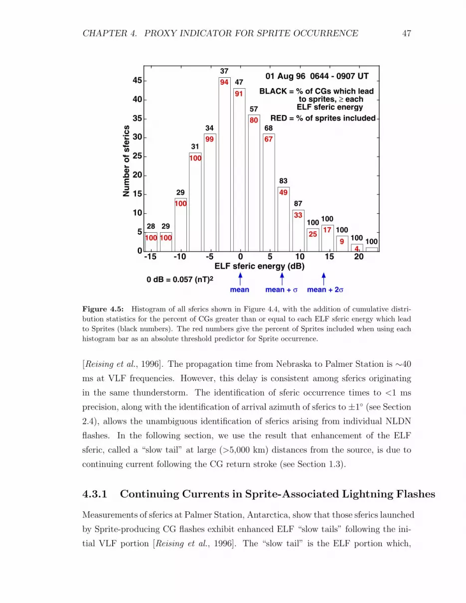
CHAPTER 4. PROXY INDICATOR FOR SPRITE OCCURRENCE 47
-15 -10 -5 0 5 10 15 200
5
10
15
20
25
30
35
40
45
28 29
29
31
34
37
47
57
68
83
87
100 100
100100 100100 100
100
100
99
94
91
80
67
49
33
25 17
9 4
BLACK = % of CGs which lead to sprites, ≥ each ELF sferic energy
Nu
mb
er o
f sf
eric
s
01 Aug 96 0644 - 0907 UT
RED = % of sprites included
ELF sferic energy (dB)
0 dB = 0.057 (nT)2mean mean + σ mean + 2σ
Figure 4.5: Histogram of all sferics shown in Figure 4.4, with the addition of cumulative distri-bution statistics for the percent of CGs greater than or equal to each ELF sferic energy which leadto Sprites (black numbers). The red numbers give the percent of Sprites included when using eachhistogram bar as an absolute threshold predictor for Sprite occurrence.
[Reising et al., 1996]. The propagation time from Nebraska to Palmer Station is ∼40
ms at VLF frequencies. However, this delay is consistent among sferics originating
in the same thunderstorm. The identification of sferic occurrence times to <1 ms
precision, along with the identification of arrival azimuth of sferics to ±1 (see Section
2.4), allows the unambiguous identification of sferics arising from individual NLDN
flashes. In the following section, we use the result that enhancement of the ELF
sferic, called a “slow tail” at large (>5,000 km) distances from the source, is due to
continuing current following the CG return stroke (see Section 1.3).
4.3.1 Continuing Currents in Sprite-Associated Lightning Flashes
Measurements of sferics at Palmer Station, Antarctica, show that those sferics launched
by Sprite-producing CG flashes exhibit enhanced ELF “slow tails” following the ini-
tial VLF portion [Reising et al., 1996]. The “slow tail” is the ELF portion which,
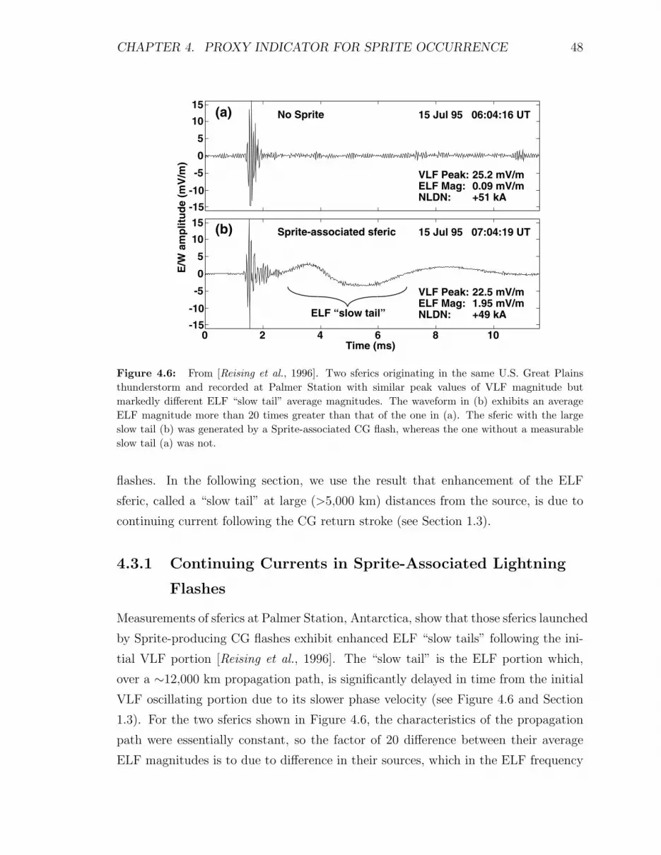
CHAPTER 4. PROXY INDICATOR FOR SPRITE OCCURRENCE 48
-15
-10
-5
0
5
10
1515 Jul 95 06:04:16 UT
E/W
am
plit
ud
e (m
V/m
)
No Sprite
VLF Peak: 25.2 mV/mELF Mag: 0.09 mV/mNLDN: +51 kA
(a)
0 2 4 6 8 10-15
-10
-5
0
5
10
1515 Jul 95 07:04:19 UT
Time (ms)
Sprite-associated sferic
VLF Peak: 22.5 mV/mELF Mag: 1.95 mV/mNLDN: +49 kA
(b)
ELF “slow tail”
Figure 4.6: From [Reising et al., 1996]. Two sferics originating in the same U.S. Great Plainsthunderstorm and recorded at Palmer Station with similar peak values of VLF magnitude butmarkedly different ELF “slow tail” average magnitudes. The waveform in (b) exhibits an averageELF magnitude more than 20 times greater than that of the one in (a). The sferic with the largeslow tail (b) was generated by a Sprite-associated CG flash, whereas the one without a measurableslow tail (a) was not.
flashes. In the following section, we use the result that enhancement of the ELF
sferic, called a “slow tail” at large (>5,000 km) distances from the source, is due to
continuing current following the CG return stroke (see Section 1.3).
4.3.1 Continuing Currents in Sprite-Associated Lightning
Flashes
Measurements of sferics at Palmer Station, Antarctica, show that those sferics launched
by Sprite-producing CG flashes exhibit enhanced ELF “slow tails” following the ini-
tial VLF portion [Reising et al., 1996]. The “slow tail” is the ELF portion which,
over a ∼12,000 km propagation path, is significantly delayed in time from the initial
VLF oscillating portion due to its slower phase velocity (see Figure 4.6 and Section
1.3). For the two sferics shown in Figure 4.6, the characteristics of the propagation
path were essentially constant, so the factor of 20 difference between their average
ELF magnitudes is to due to difference in their sources, which in the ELF frequency

CHAPTER 4. PROXY INDICATOR FOR SPRITE OCCURRENCE 49
band are continuing currents (see Section 1.3). In Figure 4.6 the sferics measurements
are displayed in terms of the electric field (E), even though the measured quantity
is the wave magnetic field (B). For ground measurements of waves propagating in
free space, the magnitudes E and B are related by E = cB, where c is the speed
of light. This relationship is also correct for the quasi-transverse electric and quasi-
transverse magnetic modes (VLF sferic) in the waveguide. For the quasi-transverse
electromagnetic mode (ELF sferic), the phase velocity is ∼0.9 c [Sukhorukov and
Stubbe, 1997], so the relationship is approximately true. Under these conditions, the
following conversion:
30mV
m⇐⇒ 0.1 nT
can be used to convert from quantities given in E for Palmer Station measurements
to quantities given in B for Yucca Ridge measurements.
The observation that those sferics launched by Sprite-producing CG flashes ex-
hibit enhanced ELF “slow tails” compared to non Sprite-producing sferics indicates
that significant continuing currents on the time scale of ∼1-5 ms are a necessary
condition for Sprite production [Reising et al., 1996]. This interpretation of slow-tail
enhancement (see Section 1.3) is consistent with the requirement of continuing cur-
rent in order to lower large amounts of charge from the cloud to ground, which is
believed to be necessary for Sprite production (see Sections 1.2.2 and 1.1).
4.3.2 Sprite-Producing Storm on July 12, 1994
Two cases studied by Reising et al. [1996] demonstrate the usefulness of the proxy in-
dicator at ∼12,000 km range from the Sprite-producing mesoscale convective system.
In the first case, on July 12, 1994, 44 Sprites were observed at Yucca Ridge between
0510 and 0712 UT, at the rate of just less than one Sprite every 3 minutes. Figure
4.7a shows the locations of all positive CG flashes recorded by NLDN, and the circles
in Figure 4.7c show the locations of those positive CGs which produced Sprites. At
Palmer, sferics were detected in association with 42 of the 44 (95%) Sprites. The
NLDN recorded positive CG flashes in 31 of the 44 (70%) events within ±100 ms of
the period between the onset of the Sprite and the end of its observed luminosity, as
recorded by the intensified CCD camera at Yucca Ridge. The peak current distribu-
tion of these 31 flashes is shown in shaded bars in the left panel of Figure 4.8. These
Sprite-associated CGs have a wide variation of peak currents, nearly spanning the

CHAPTER 4. PROXY INDICATOR FOR SPRITE OCCURRENCE 50
-106 -104 -102 -100 -98 -96 -94
38
40
42
Longitude (deg E)
Lat
itu
de
(deg
N)
YR
Case B15 Jul 95 0545-0732 UT
Longitude (deg E)-94-106 -104 -102 -100 -98 -96
38
40
42
44
46
YR
-30˚ -28˚ -26˚Bearings from PA
15 Jul 950545-0732 UT
-106 -104 -102 -100 -98
38
40
Longitude (deg E)
YR
Case A12 Jul 94 0510-0712 UT
Longitude (deg E)-106 -104 -102 -100 -98
38
40
42
44
YR
-30˚ -28˚
Bearings from PA
12 Jul 940510-0712 UT
Lat
itu
de
(deg
N)
ALL +CGs> 60 kA> 30 kA < 30 kA
(c)
(a)
(d)
(b)
15 Jul 9512 Jul 94
ALL +CGs> 60 kA> 30 kA < 30 kA
Figure 4.7: From [Reising et al., 1996]. Panel (a) shows all positive CG flashes recorded by NLDNfrom a mesoscale convective system in central/SW Nebraska and NE Colorado, from 0510-0712 UTon July 12, 1994. The locations of Sprite-producing positive CGs recorded by NLDN are denotedby circles in (c). Panel (b) shows the positive CG flashes from 0545-0732 UT on July 15, 1995, froma mesoscale convective system with strong activity in central/SW Nebraska, with weaker positiveCGs in Iowa. Sprite-producing positive CGs are shown as circles in panel (d). The intensified CCDcamera fields-of-view are shown as rays extending from Yucca Ridge (YR). The dotted lines are linesof constant bearing from Palmer Station, Antarctica. The NLDN data is provided by courtesy ofNASA/MSFC and the Global Hydrology Resource Center.

CHAPTER 4. PROXY INDICATOR FOR SPRITE OCCURRENCE 51
NLDN estimated peak current (kA) ELF sferic energy (dB); 0 dB = 3.651 (pT)2 10 20 50 100 200
0
5
10
15N
um
ber
of
flas
hes
(sf
eric
s) NLDN 12 Jul 940510-0712 UT
-20 -10 0 10 200
5
10
15 ELF sferic energy 12 Jul 940510-0712 UT
Figure 4.8: Adapted from [Reising et al., 1996]. Distributions of NLDN peak current (left panel)and corresponding Palmer ELF sferic energy (right panel) for all 144 positive CGs on July 12, 1994,within the intensified CCD camera field-of-view. The vertical scales are number of first strokes forthe left panel, and number of sferics for the right panel. Sprite-associated CGs are shown as shadedbars, and non Sprite-associated CGs are shown as unshaded bars.
entire distribution of 144 positive CGs within the field of view (shown as unshaded
bars). The ELF sferic energy distribution of the same 144 positive CGs is shown in
the right panel of Figure 4.8, with the 31 Sprite-associated CGs denoted by shaded
bars. The ELF sferic energy is an average over the first 10 ms of the sferic, as in Reis-
ing et al. [1996]. The distribution demonstrates that Sprite-producing CGs generate
sferics with large ELF energy, indicative of large continuing currents on the time scale
of several milliseconds [Reising et al., 1996].
4.3.3 Sprite-Producing Storm on July 15, 1995
In the second case, on July 15, 1995, 35 Sprites were observed at Yucca Ridge between
0545 and 0732 UT, at the rate of one Sprite every ∼3 minutes. Figure 4.7b shows
the locations of all positive CG flashes recorded by NLDN, and the circles in Figure
4.7d give the locations of those positive CGs which produced Sprites. At Palmer
Station, sferics were detected in association with 34 of the 35 (97%) Sprites. The
NLDN recorded positive CG flashes in 29 of the 35 (83%) events within ±100 ms of
the period between the onset of the Sprite and the end of its observed luminosity.
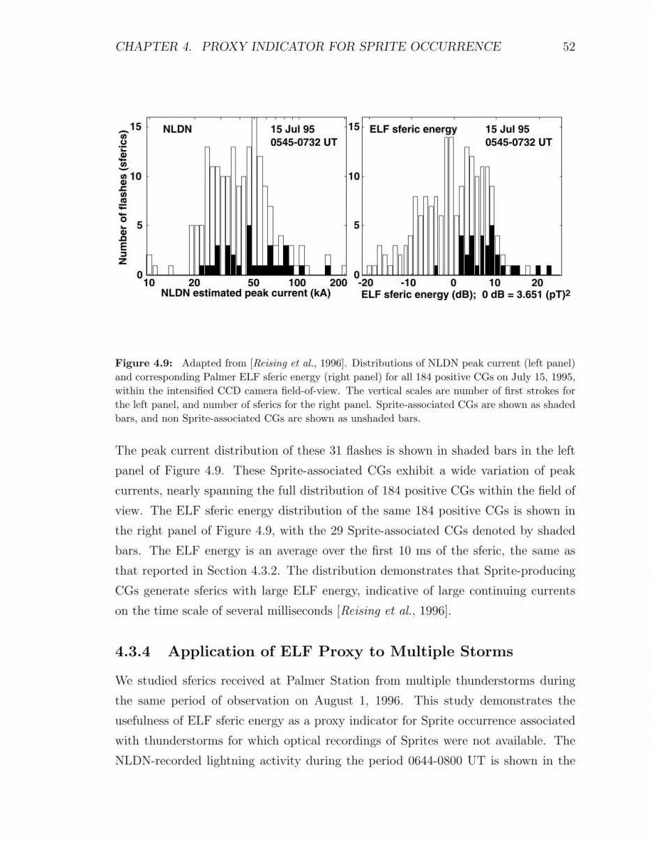
CHAPTER 4. PROXY INDICATOR FOR SPRITE OCCURRENCE 52
10 20 50 100 2000
5
10
15N
um
ber
of
flas
hes
(sf
eric
s)
NLDN estimated peak current (kA)
NLDN 15 Jul 950545-0732 UT
-20 -10 0 10 200
5
10
15
ELF sferic energy (dB); 0 dB = 3.651 (pT)2
ELF sferic energy 15 Jul 950545-0732 UT
Figure 4.9: Adapted from [Reising et al., 1996]. Distributions of NLDN peak current (left panel)and corresponding Palmer ELF sferic energy (right panel) for all 184 positive CGs on July 15, 1995,within the intensified CCD camera field-of-view. The vertical scales are number of first strokes forthe left panel, and number of sferics for the right panel. Sprite-associated CGs are shown as shadedbars, and non Sprite-associated CGs are shown as unshaded bars.
The peak current distribution of these 31 flashes is shown in shaded bars in the left
panel of Figure 4.9. These Sprite-associated CGs exhibit a wide variation of peak
currents, nearly spanning the full distribution of 184 positive CGs within the field of
view. The ELF sferic energy distribution of the same 184 positive CGs is shown in
the right panel of Figure 4.9, with the 29 Sprite-associated CGs denoted by shaded
bars. The ELF energy is an average over the first 10 ms of the sferic, the same as
that reported in Section 4.3.2. The distribution demonstrates that Sprite-producing
CGs generate sferics with large ELF energy, indicative of large continuing currents
on the time scale of several milliseconds [Reising et al., 1996].
4.3.4 Application of ELF Proxy to Multiple Storms
We studied sferics received at Palmer Station from multiple thunderstorms during
the same period of observation on August 1, 1996. This study demonstrates the
usefulness of ELF sferic energy as a proxy indicator for Sprite occurrence associated
with thunderstorms for which optical recordings of Sprites were not available. The
NLDN-recorded lightning activity during the period 0644-0800 UT is shown in the

CHAPTER 4. PROXY INDICATOR FOR SPRITE OCCURRENCE 53
0
5
10
15
0
5
10
15
-10 -5 0 5 10 15 200
5
10
15
ELF sferic energy (dB); 0 dB = 0.80 (pT)2
Storm AShaded = Observed Sprites
Storm B Shaded = Predicted Sprites
Storm CNo Sprites
Nu
mb
er o
f sf
eric
s
Storm B
Storm C
YuccaRidge
Storm A
30˚N
45˚ N
120˚ W
90˚ W
Figure 4.10: (Left) Locations of positive cloud-to-ground flashes observed by the NLDN with peakcurrent exceeding 23 kA from 0644-0800 UT on August 1, 1996, identical to Figure 2.7. (Right)Distributions of ELF sferic energy for sferics recorded at Palmer from Storms A, B and C from 0644to 0745 UT on August 1, 1996. All sferics are generated by positive CGs recorded by the NLDN withpeak current ≥23 kA. In the top panel, shaded bars indicate Sprite-associated sferics, as verified byoptical observations at Yucca Ridge (see Section 3.2).
left panel of Figure 4.10, where pluses denote positive CG flashes with peak currents
exceeding 23 kA. Storm A is the Sprite-producing storm in western Kansas described
in detail in Sections 3.2 and 4.2. Storm B is in Sonora, Mexico, just to the east of the
Gulf of California. Storm C is a smaller thunderstorm in South Dakota. The GOES
8 infrared brightness temperature data at 0702 UT for the same region is shown in
Figure 4.11. The areas of coldest cloud tops are shown in purple and white (Storms
A and B), indicating the presence of mixed-phase regions, which are known to be
important for thunderstorm electrification and for the generation of large stratiform
regions, above which Sprites are observed to occur (see Section 1.2.5).
By matching arrival azimuth and propagation delay separately for each storm
(see Section 2.4), we measured sferics in association with many of the NLDN positive
CGs with peak currents >23 kA, for storms A, B and C (see Figure 4.10). The
distributions of ELF sferic energy for sferics measured from 0644 to 0745 UT in each
of the three storms are shown in the right panel of Figure 4.10. In this case the ELF

CHAPTER 4. PROXY INDICATOR FOR SPRITE OCCURRENCE 54
energy is an average over the first 20 ms of the sferic, as in Section 4.2, so the mean
sferic energy is smaller than that shown in Figures 4.8 and 4.9. In the top right panel
of Figure 4.10, the shaded bars show the ELF energy of sferics generated by Sprite-
associated positive CGs, as determined from optical measurements at Yucca Ridge.
Storm B shows an overall distribution which is similar to Storm A, and we infer from
the sferic energy distribution of the detected Sprites in Storm A that Storm B most
likely produced at least as many Sprites as shown by the shaded bars in the middle
right panel. We note that Sprites were measured optically during the summer of 1997
above storms in the same region as Storm B, with a higher rate of Sprite production
than many of the Great Plains storms [Barrington-Leigh et al., 1997]. Storm C was a
smaller storm with a lower rate of positive CGs, and our measurements indicate that
it produced very few or no Sprites at all.
Based on ground-based observations of thousands of Sprites, Lyons [1996] gives
meteorological criteria for thunderstorms in the U.S. Great Plains which are likely
to produce Sprites. His initial evidence indicates that a necessary, but not sufficient,
condition for Sprite production is a mesoscale convective system with >20,000 km2
radar echo area having a large stratiform precipitation region containing numerous
positive CG flashes [Lyons, 1996]. Storm A meets these criteria, and Storm B has
radar echoes >100,000 km2, putting it into the category of a mesoscale convective
complex (see Section 1.2.5). Storm C covers >60,000 km2, but it has only 0.25
positive CGs per minute during this period, as opposed to 0.6 and 1.7 positive CGs
per minute in Storm B and Storm A, respectively. The flash rate in Storm B is likely
greater than the 0.6 positive CGs per minute measured by NLDN, because Storm B
is located near the edge of the NLDN coverage area [Cummins et al., 1998]. Sprites
have been observed above smaller thunderstorms in Florida [Stanley et al., 1997] and
in South America [Sentman et al., 1996], so, as Lyons [1996] points out, the criteria
for a Sprite-producing thunderstorm need to be modified for different climatological
regimes.
4.4 ELF Radiation from Electrical Currents in Sprites
In this section we return to analysis of sferics measurements performed at Yucca Ridge
during Summer 1996, at ∼500-600 km distance from Sprite-producing mesoscale con-
vective systems in Kansas and Nebraska. At this range, the ELF component of a
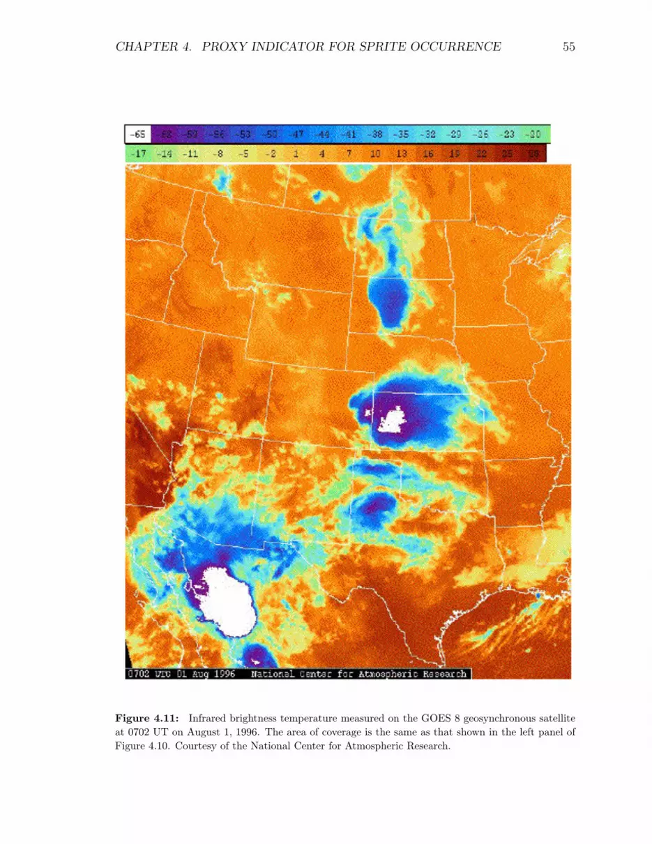
CHAPTER 4. PROXY INDICATOR FOR SPRITE OCCURRENCE 55
Figure 4.11: Infrared brightness temperature measured on the GOES 8 geosynchronous satelliteat 0702 UT on August 1, 1996. The area of coverage is the same as that shown in the left panel ofFigure 4.10. Courtesy of the National Center for Atmospheric Research.

CHAPTER 4. PROXY INDICATOR FOR SPRITE OCCURRENCE 56
0
20
40
E/W
am
pl.
(nT
)
0 1 2 3 4 5 6
0
5
10
Time (ms)
EL
F a
mp
l. (n
T)
Sferic: 08:26:09.95 UT
NLDN: +164 kA Yucca Ridge
ELF Sferic: 08:26:09.95 UT
-5
0
5
10
15
E/W
am
pl.
(nT
)
0 1 2 3 4 5 6-4
0
4
8
Time (ms)
EL
F a
mp
l. (n
T)
08:24:00.12 UT
NLDN: +67 kA Yucca Ridge
ELF Sferic1.5 kHz LPF1.5 kHz LPF
Figure 4.12: (Top Left) The sferic waveform launched by a 164-kA positive CG discharge andmeasured at Yucca Ridge at 08:26:09 UT on August 1, 1996. (Top Right) The sferic waveformlaunched by a 67-kA positive CG discharge and measured at Yucca Ridge at 08:24:00 UT on August1, 1996. (Bottom Panels) The ELF components of both sferics after digital lowpass filtering with acutoff frequency of 1.5 kHz.
typical Sprite-associated sferic consists of a positive-going pulse of half width 0.5-
1 ms followed by a negative-going pulse of much smaller magnitude which recovers to
zero in <20 ms, as shown in the lower left panel of Figure 4.12. However, in ∼20%
of the Sprite-associated sferics, a second positive-going ELF pulse is observed, clearly
separated in time from the first positive ELF pulse, as shown in the lower right panel
of Figure 4.12. Simultaneous photometric observations of Sprite luminosity at high
time resolution (∼30 µs) verified that the Sprite luminosity rises and falls nearly si-
multaneous with the source current which radiated the second ELF pulse [Cummer
et al., 1998]. The lack of a VLF oscillation at the beginning of the second ELF pulse
(see top right panel of Figure 4.12) indicates that this pulse is not generated by a CG
return stroke nor by an intracloud lightning discharge. The authors conclude that
the temporal association strongly suggests that the source of the second ELF pulse
is current flowing in the body of the Sprite itself. In the context of our study, it is
important to recognize that the second ELF pulse is included in the proxy indicator
described in Section 4.2. As seen in Figure 4.4, the ELF energy distribution of Sprite
associated sferics is not strictly Gaussian, but rather bimodal, where the rightmost
peak is likely influenced by the presence of the second ELF pulse. This effect is not
observed in Figures 4.8 and 4.9 because the time window for measurement of ELF
energy extends to t = 10 ms, as opposed to t = 20 ms for Figure 4.4. Secondly, at
∼12,000 km propagation distance the ELF slow tail is delayed by ∼3 ms from the

CHAPTER 4. PROXY INDICATOR FOR SPRITE OCCURRENCE 57
-5
0
5
10
15
E/W
am
plit
ud
e (n
T)
Sferic: 08:24:00.12 UT - 60 Hz removed
-4-2
0
24
6
8
EL
F a
mp
litu
de
(nT
)
ELF Sferic: 08:24:00.12 UT - 1.5 kHz LPF
-2 0 2 4 6 8 10
4
6
8
Time (ms)
#11
Inte
nsi
ty (
MR
)NLDN: +67 kA Yucca Ridge
Fly's Eyephotometer data
94 km
46 km
Figure 4.13: (Top) The sferic waveform launched by a 67-kA positive CG discharge and measuredat Yucca Ridge at 08:24:00 UT on August 1, 1996. (Middle) The ELF component of the same sfericafter digital lowpass filtering with a cutoff frequency of 1.5 kHz. (Bottom) Optical intensity datameasured by the Fly’s Eye photometer #11. The inset shows the field of view of the photometer bydotted lines overlaid on the image of the Sprite associated with this sferic.
VLF onset, so many of the second ELF pulses are delayed past t = 10 ms.
We present simultaneous photometric and sferic observations made at Yucca Ridge
of Sprites and lightning produced by the mesoscale convective system in western
Kansas on August 1, 1996 (see Section 4.2), which are consistent with the results
of Cummer et al. [1998]. Photometric observations were conducted with an array
of photometers as part of the Stanford / Lockheed Fly’s Eye experiment [Inan et
al., 1997]. This array consisted of Hamamatsu HC124-01 integrated photomultiplier
assemblies with light shields, lenses, and precision-cut focal-plane screens to provide
specific views of the sky [Inan et al., 1997]. In this work we show results from
photometer #11, which had a 6.6 wide by 3.3 high field of view, denoted by dotted
lines on the inset in Figure 4.13. This figure shows a sferic launched by a 67-kA

CHAPTER 4. PROXY INDICATOR FOR SPRITE OCCURRENCE 58
0
5
10
EL
F a
mp
litu
de
(nT
)
ELF Sferic: 08:39:30.30 UT - 1.5 kHz LPF
-2 0 2 4 6 8 10
5
10
15
20
Time (ms)
#11
Inte
nsi
ty (
MR
)
-5
0
5
10
15
20
E/W
am
plit
ud
e (n
T)
Sferic: 08:39:30.30 UT - 60 Hz removed
NLDN : +83 kA Yucca Ridge
Fly's Eyephotometer data
90 km
55 km
Figure 4.14: (Top) The sferic waveform launched by a 83-kA positive CG discharge and measuredat Yucca Ridge at 08:39:30 UT on August 1, 1996. (Middle) The ELF component of the same sfericafter digital lowpass filtering with a cutoff frequency of 1.5 kHz. (Bottom) Optical intensity datameasured by the Fly’s Eye photometer # 11. The inset shows the field of view of the photometerby dotted lines overlaid on the image of the Sprite associated with this sferic.
positive CG at 08:24:00 UT (top panel), the ELF component of the sferic (middle
panel) and the photometer #11 data (bottom panel) showing Sprite luminosity (see
inset). These data confirm simultaneity (within ±0.2 ms) of the second pulse of the
ELF sferic and the Sprite luminosity, consistent with Cummer et al. [1998]. The
second ELF pulse has slightly larger amplitude and longer duration than the first,
indicating a larger charge-moment associated with the charge transfer in the Sprite
than in the cloud-to-ground continuing current which produced the first pulse. A
second example is the sferic launched by a 83-kA positive CG at 08:39:30 UT presented
in Figure 4.14, in the same format as this previous figure. In this case the second
pulse is of much smaller amplitude than the first, but the simultaneity of the second
ELF pulse and the Sprite luminosity is again apparent.

CHAPTER 4. PROXY INDICATOR FOR SPRITE OCCURRENCE 59
0 50 100 150 200 250 300 350 4000
50
100
150
200
250
Sprite charge moment (C-km)
Approximately linear variation
Saturation
To
tal S
pri
te lu
min
osi
ty (
un
calib
rate
d)
Figure 4.15: The quantitative relationship of Sprite charge moment and total Sprite luminosityfor 17 Sprites on July 24, 1996. The moment of charge transfer in the Sprite is inferred from thesecond ELF pulse, as measured at Yucca Ridge. The Sprite luminosity is calculated from intensifiedCCD video recordings of Sprites, as observed at Yucca Ridge.
The dipole moment associated with charge transfer in the source of the second
ELF pulse can be calculated using a method applied to estimation of the continuing
current from the first ELF pulse by Bell et al. [1996; 1998] and discussed in Section
3.3. To obtain a lower bound for the moment of charge transfer in the Sprite itself,
we reduced the calculated charge moment by 25% because some of the energy in
the second ELF pulse may be generated by weak continuing currents flowing from
the cloud to the ground at the time of Sprite occurrence, as suggested by Cummer
et al. [1998]. We applied this procedure to sferics measurements on July 24, 1996,
from an unusually extensive mesoscale convective system covering western Kansas
and Oklahoma, and extending deep into the Texas panhandle. Video observations at
Yucca Ridge on July 24 recorded at least 140 Sprites from 05:19 to 08:56 UT, giving
a rate of one Sprite every ∼90 seconds, occurring to the southeast at ∼500-650 km
range from Yucca Ridge. Several interesting sequences were recorded on July 24,

CHAPTER 4. PROXY INDICATOR FOR SPRITE OCCURRENCE 60
-1
0
1
2N
/S a
mp
litu
de
(nT
)
0 10 20 30 40 50 60-0.5
0
0.5
1
EL
F a
mp
litu
de
(nT
)
Time (ms)
Sferic: 07:43:48.840 UT - 60 Hz removed
NLDN: +48 kA Yucca Ridge
ELF Sferic: 07:43:48.840 UT - 1.5 kHz LPF
Figure 4.16: (Top) The sferic waveform launched by a 48-kA positive CG discharge and measuredat Yucca Ridge at 07:43:48 UT on July 24, 1996. (Bottom) The ELF component of the same sfericafter digital lowpass filtering with a cutoff frequency of 1.5 kHz.
where up to eight Sprites appear to “dance” laterally across the camera field of view
in a duration of only 0.5-1.0 seconds (e.g., [Nelson et al., 1997]).
On July 24, at least 17 Sprite-associated sferics exhibited second ELF pulses.
Using simultaneous intensified CCD camera images, we measured the total Sprite
luminosity as the product of the number of Sprite-illuminated CCD pixels and the
average luminosity in each of those pixels. To compensate for varying range between
the camera and the Sprite, the measurement was scaled by the square of the range
from the camera to the Sprite-associated CG. The assumption of Sprite occurrence
near the location of its associated CG has been shown to be valid to within ∼40 km
in most cases [Winckler et al., 1996; Lyons, 1996], and was used to assign altitude
scales to all of the Sprite images shown in this chapter. For these 17 cases, we show
an approximately linear relationship between Sprite charge moment and total Sprite
luminosity in Figure 4.15. The Sprite luminosity exhibits saturation at the largest
two values of Sprite charge moment. The individual CCD pixels were not saturated,
so further data are needed to establish the physical cause of the saturation.
The circles in Figure 4.15 denote two examples in which the delay between the
occurrence of the associated positive CG and the Sprite onset is >50 ms. In all other

CHAPTER 4. PROXY INDICATOR FOR SPRITE OCCURRENCE 61
54 55 56 57 58 59 60 61-0.5
0
0.5
1N/S Signal - 1.5 kHz LPF
Yucca Ridge Data: 24 Jul 96 07:43:48.840 UT; NLDN: Ipeak = +48 kA
EL
F a
mp
litu
de
(nT
)
Time (ms)
Multi-Anode Photometer: 24 Jul 96 07:43:48.894 UT
Rel
ativ
e In
ten
sity
Yucca Ridge Data: 24 Jul 96 07:43:48.840 UT (t=0)
NLDN: +48 kA
ELF Sferic - 1.5 kHz LPF
#10
#8
#6
96 km
47 km
Figure 4.17: (Top) The optical intensity of the Sprite at 07:43:48 UT on July 24, 1996, as recordedby the multi-anode photometer channels #6-10 (Courtesy of Dr. Y. Takahashi). The fields of viewof the multi-anode photometer channels are indicated by dotted lines in the associated Sprite imageat right. (Bottom) A time-expanded view of the bottom panel of Figure 4.16 from t = ∼54 tot = 62 ms, including the second ELF pulse.
cases shown in Figure 4.15, the CG-to-Sprite delay was <18 ms. For the two cases
of >50 ms delay, we compared ELF sferics to simultaneous data from multi-anode
photometer measurements performed at Yucca Ridge by our colleagues from Tohoku
University in Sendai, Japan [Takahashi et al., 1997]. The multi-anode photometer
instrument was deployed to resolve the vertical development of Sprites at high time
resolution (∼20 µs). The instrument consists of a 16-element vertical column of
photometers, each of which has a ∼9 wide by 1 high field of view (see right panel of
Figure 4.17). Figure 4.16 shows a sferic produced by a 48-kA positive CG at 07:43:48
UT on July 24, 1996, and measured at Yucca Ridge. The lower panel shows the ELF
sferic, where the first ELF pulse follows the return stroke (in <1 ms), and the second
ELF pulse occurs ∼56 ms later. The high signal-to-noise ratio of the Yucca Ridge
observations is evident, even for a modest-sized positive CG of 48 kA, and the peak

CHAPTER 4. PROXY INDICATOR FOR SPRITE OCCURRENCE 62
-2
0
2
4
6
Sferic: 07:37:51.044 UT - 60 Hz removed
NLDN: +72 kA Yucca RidgeN
/S a
mp
litu
de
(nT
)
0 10 20 30 40 50 60 70-1
0
1
2
EL
F a
mp
litu
de
(nT
)
Time (ms)
ELF Sferic: 07:37:51.044 UT - 1.5 kHz LPF
Figure 4.18: (Top) The sferic waveform launched by a 72-kA positive CG discharge and measuredat Yucca Ridge at 07:37:51 UT on July 24, 1996. (Bottom) The ELF component of the same sfericafter digital lowpass filtering with a cutoff frequency of 1.5 kHz.
amplitude of the second ELF pulse is about 70% of that of the first ELF pulse. An
expanded view of the second ELF pulse on ∼8 ms time scale is shown in the bottom
panel of Figure 4.17. The upper panel shows the intensity measurements of channels
#6-10 of the multi-anode photometer on the same time scale, with corresponding
fields of view as delineated by dotted lines in the image on the right [Takahashi et al.,
1997]. The second ELF pulse occurs simultaneously with the Sprite luminosity and
has a similar form to the optical data from channels #6 and #7, consistent with the
results shown in Figures 4.13 and 4.14. Figure 4.18 shows a sferic waveform produced
by a 72-kA positive CG at 07:37:51 UT. The lower panel shows the ELF sferic, where
the second ELF pulse lags the first ELF pulse by ∼70 ms and reaches approximately
half its peak amplitude. The multi-anode photometer signatures and ELF data are
shown on identical time axes in Figure 4.19. The second ELF pulse exhibits a similar
time development to the luminosity recorded by multi-anode photometer channel #9.
The coincident photometric and sferic measurements presented in Figures 4.13,
4.14, 4.17, and 4.19 show that the second ELF pulse occurs at the time of Sprite
appearance to better than ±0.2 ms. Every observation of the second ELF pulse in
the Yucca Ridge continuous sferic data has two characteristics: (1) it is accompanied

CHAPTER 4. PROXY INDICATOR FOR SPRITE OCCURRENCE 63
64 65 66 67 68 69 70 71 72 73 74 75 76-0.5
0
0.5
1 N/S Signal - 1.5 kHz LPF
Yucca Ridge Data: 24 Jul 96 07:37:51.044 UT; NLDN: Ipeak = +72 kA
EL
F a
mp
litu
de
(nT
)
Time (ms)
Multi-Anode Photometer: 24 Jul 96 07:37:51.108 UT
Yucca Ridge Data: 24 Jul 96 07:37:51.044 UT (t=0)
Rel
ativ
e In
ten
sity
NLDN: +72 kA
ELF Sferic - 1.5 kHz LPF
#10
#8
#6
95 km
45 km
Figure 4.19: (Top) The optical intensity of the Sprite at 07:37:51 UT on July 24, 1996, as recordedby the multi-anode photometer channels #6-10 (Courtesy of Dr. Y. Takahashi). The fields of viewof the multi-anode photometer channels are indicated by dotted lines in the associated Sprite imageat right. (Bottom) A time-expanded view of the bottom panel of Figure 4.18 from t = ∼63 to t =∼76 ms, including the second ELF pulse.
by the occurrence of a Sprite, and (2) it is not accompanied by a VLF oscillation at
its onset, as opposed to sferics generated by conventional lightning discharges [Inan et
al., 1996b; Reising et al., 1996; Cummer et al., 1998]. Consequently, every occurrence
of the second ELF pulse allows measurement of the delay between the positive CG
and Sprite onset with ±0.2 ms precision. The second ELF pulse is clearly observed at
Yucca Ridge in ∼20% of Sprite cases detected by the intensified CCD camera. This
measurement of the CG-to-Sprite delay is nearly 50 times more precise than the 16.7
ms resolution provided by intensified CCD measurements (see Section 3.3).
In order to verify and extend the results of Bell et al. [1998], we identified 17
sferics on July 24, 1996, which had a clearly observed second ELF pulse and which
were associated with optically detected Sprites. To find the relationship between
CG-to-Sprite delay and continuing current following each positive CG, we applied
the method of Bell et al. [1996; 1998] (see Section 3.3) to the first ELF pulse to

CHAPTER 4. PROXY INDICATOR FOR SPRITE OCCURRENCE 64
0 2 4 6 8 10 12 14 16 180
200
400
600
800
1000
1200
Time delay between CG and second ELF pulse (ms)
Clo
ud
-to
-gro
un
d c
har
ge
mo
men
t (C
-km
)
Figure 4.20: The relationship of continuing current charge moment and CG-to-Sprite delay for17 Sprites on July 24, 1996. The moment of positive charge transfer from the cloud to the ground inthe continuing current is inferred from measurements at Yucca Ridge of the first ELF pulse of eachsferic. The CG-to-Sprite delay is the time between the peak of the first ELF pulse (within 1 ms ofsferic onset) and the peak of the second ELF pulse.
obtain an estimate of the charge moment in the continuing current. The results for
the 17 cases analyzed are shown in Figure 4.20. If the length of the cloud-to-ground
channel is 10 km, these values range from ∼10 to 120 C. In all cases with charge
transfer exceeding 30 C, the CG-to-Sprite delay was <4.5 ms. For smaller charge
transfers (<25 C), the delay time until Sprite appearance ranges from ∼4 to 17 ms
for this data set. From the two examples shown in Figures 4.16 to 4.19, we know
that the maximum delay may be as large as 50-70 ms. These results indicate that if
a large quantity of charge is lowered from the cloud to the ground in the continuing
current, then a Sprite is produced in <5 ms. Smaller charge transfers to ground in
the continuing current may require associated, yet weaker, intracloud currents to flow
for a longer time in order to move sufficient positive charge for Sprite production (see
Sections 1.2.5 and 3.3). These results agree with those of Bell et al. [1998] and extend
their measurements of CG-to-Sprite delay to sub-millisecond time precision.

Chapter 5
Summary and Suggestions for
Future Work
5.1 Summary
Novel digital signal processing techniques were developed for automated identifica-
tion and arrival azimuth determination of radio atmospherics (“sferics”) in broad-
band ELF/VLF data on a continuous basis. Sferics are identified in the presence of
non-stationary interference produced by natural and anthropogenic sources, based on
criteria of threshold intensity and of coherence among multiple sensors. Identifica-
tion of the time of occurrence of sferics to ∼1 ms precision allows the identification
of individual lightning discharges as the sources of individual sferics. The arrival
azimuth of each sferic is determined using the VLF Fourier Goniometry technique
[Burgess, 1993]. Based on broadband ELF/VLF measurements at Palmer Station,
Antarctica, we measure the arrival azimuths of individual sferics and compare them
with the expected arrival azimuths based on known locations of the individual source
lightning discharges. The locations of lightning flashes in the continental U.S. are
identified by the National Lightning Detection Network (NLDN) within ∼0.5 km
precision. Comparison of expected and measured arrival azimuths demonstrates ar-
rival azimuth determination to ±1 precision for sferics propagating from Nebraska
to Palmer Station, Antarctica, a source-to-receiver distance of ∼12,000 km.
Broadband ELF/VLF measurements of sferics at Palmer Station, Antarctica,
show that the ELF “slow tails” of Sprite-associated sferics have large energy in relation
65

CHAPTER 5. SUMMARY AND SUGGESTIONS FOR FUTURE WORK 66
to the slow tails of non Sprite-associated sferics at a range of ∼12,000 km [Reising
et al., 1996]. Since ELF slow tails are enhanced by continuing current flowing on
∼1-3 ms time scales, these measurements provide the first evidence that continuing
currents are a necessary component of those positive cloud-to-ground (CG) discharges
which lead to Sprite production [Reising et al., 1996]. Continuing current of >1 ms
duration after the first return stroke of a flash is necessary to transfer >120 C of charge
from the cloud to the ground. Evidence for continuing current in Sprite-producing
lightning flashes is consistent with predictions based on quasi-electrostatic models of
Sprite production. Pasko et al. [1997] predict that the cloud-to-ground charge mo-
ment change in a lightning discharge must exceed a threshold value in order for a
Sprite to be produced.
Broadband ELF/VLF measurements of sferics near Ft. Collins, Colorado, demon-
strate that the ELF sferic energy is a proxy indicator for Sprite occurrence that can be
used to estimate the number of Sprites produced by a thunderstorm with an accuracy
of ±25%. Our results are in agreement with previous criteria for Sprite-producing
thunderstorms in the U.S. Great Plains [Lyons, 1996], extend these predictions to
other geographical regions and provide an estimate of the number of Sprites pro-
duced by each thunderstorm.
Video observations of Sprites, simultaneous with broadband ELF/VLF measure-
ments, confirm that Sprites are uniquely associated with positive CG lightning flashes.
The identification of Sprite onset time with ∼17 ms resolution reveals variable de-
lays of 1-100 ms between the positive CG lightning discharge and the Sprite [Bell
et al., 1996; 1998]. When photometer measurements are available, they enable the
identification of Sprite onset time with sub-millisecond resolution. Comparison of
photometer measurements and ELF sferics demonstrates the simultaneity of Sprite
luminosity and an ELF “second pulse” radiated by currents within the body of the
Sprite [Cummer et al., 1998]. In our study, we confirm the simultaneity of Sprite lu-
minosity and the ELF second pulse in cases where the Sprite is delayed by 50-70 ms
after the Sprite-associated positive CG. Our measurements of the ELF second pulse
are used to identify an approximately linear relationship between the current within
the Sprite body and the total luminosity of the Sprite.
Measurements of sferics from multiple storms at Palmer Station, Antarctica, show
that the ELF sferic energy is a useful indicator of Sprite occurrence, even at large
distances (∼12,000 km) from the source lightning. Video observations are not always

CHAPTER 5. SUMMARY AND SUGGESTIONS FOR FUTURE WORK 67
practical, so the proxy indicator is needed for identification of Sprite-producing storms
and assessment of Sprite occurrence rates on a global basis. Our results suggest that
a few appropriately placed ELF/VLF sferics receivers are sufficient for estimation of
global Sprite occurrence rates.
5.2 Suggestions for Future Work
5.2.1 Assessment of the Global Distribution of Sprite
Occurrence
Sprites have been measured from the ground over thunderstorms in the U.S. Great
Plains [Lyons, 1996], the Midwest [Winckler et al., 1996], Florida [Stanley et al., 1997],
Mexico [Barrington-Leigh et al., 1997] and northern Australia [R. Dowden, personal
communication, 1997]. In addition, Sprites have been measured from aircraft over the
central U.S. [Sentman et al., 1995] and over Central America and Peru [Sentman et
al., 1996]. Observations from the Space Shuttle have revealed Sprite occurrence over
thunderstorms in equatorial Africa, Brazil and central South America, Indonesia and
northern Australia [Boeck et al., 1995]. However, with fewer than 20 observations of
Sprites, the sample size of the Space Shuttle data is too small for assessment of the
geographical distribution of Sprite occurrence.
Since continuous optical monitoring of Sprite occurrence on large spatial scales is
not practical, an alternative proxy indicator for Sprite occurrence is needed. Mea-
surements of the ELF energy of sferics can be used as a proxy indicator for Sprite
occurrence over large areas of the Earth. A multistation sferics network can be imple-
mented to identify the storm of origin for each detected sferic, as described in Section
2.4. The proxy indicator can provide estimates of Sprite occurrence at ranges of at
least ∼12,000 km (see Section 4.3.4). As a result, the global rate of Sprite occur-
rence can be assessed from a coordinated four or five station network of broadband
ELF/VLF receivers (see Section 5.2.3).
The global rate of Sprite occurrence is needed in order to assess the global effect of
the electrodynamic coupling of lightning energy to the mesosphere and to the lower
ionosphere. The runaway acceleration of electrons [Bell et al., 1995] and ambient
electron heating [Pasko et al., 1997] which participate in the creation of the opti-
cal emissions of Sprites may also influence reaction rates and lead to the production

CHAPTER 5. SUMMARY AND SUGGESTIONS FOR FUTURE WORK 68
of different types of ions, potentially affecting mesospheric chemistry and dynamics.
Additionally, quasi-electrostatic thundercloud fields may maintain the ionosphere at
a persistently heated level [Inan et al., 1996d], possibly producing persistent infrared
glow [Picard et al., 1997], and affecting ionospheric chemistry and dynamics. Assess-
ment of these global effects requires knowledge of the occurrence of Sprites and of
the characteristics of their associated lightning discharges. This can be accomplished
on a global scale using a network consisting of a few appropriately placed broadband
ELF/VLF receivers.
5.2.2 ELF/VLF Proxy Indicator for the Occurrence of Elves
Using methods similar to those discussed in Chapter 4 of this dissertation, a proxy
indicator for the occurrence of elves may be developed and verified. “Elves” are
optical emissions produced in the lower ionosphere (∼80-95 km altitude) which de-
velop on sub-millisecond time scales and which have horizontal extents of at least
300 km and possibly as large as 600 km [Boeck et al., 1992; Inan et al., 1997]. Elves
are thought to be produced by the heating of lower ionospheric electrons by electro-
magnetic pulses produced by lightning [Inan et al., 1996c; Glukhov and Inan, 1996],
and predictions based on that mechanism agree with measurements of the rate of
horizontal expansion of elves performed as part of the Stanford University Fly’s Eye
Experiment [Inan et al., 1997]. Even though their peak brightness is similar to that of
Sprites [Fukunishi et al., 1996], elves are more difficult to identify based on low light
level video observations because of their extremely short duration compared to the
∼17 ms integration times of conventional video cameras. Consequently, validation of
any proxy indicator developed from ELF/VLF measurements of sferics requires the
use of a data set for which existence or absence of elves is clearly verifiable. Example
data sets are the Fly’s Eye photometer data [Barrington-Leigh et al., 1997] and multi-
anode photometer data conducted by experimenters at Tohoku University [Takahashi
et al., 1997]. The optical intensity threshold for detection of elves depends upon the
particular instrument used. Improvements in sensitivity were accomplished by using
a red-sensitive filter to modify the broadband response of standard photomultiplier
tubes [Inan et al., 1997; Barrington-Leigh et al., 1997]. It is likely that only a subset
of elves is detectable with current instruments and that further improvements will
result in the discovery of lower-luminosity elves.

CHAPTER 5. SUMMARY AND SUGGESTIONS FOR FUTURE WORK 69
Elves were observed first in association with positive CGs, but recent measure-
ments show association with negative CGs as well [Barrington-Leigh et al., 1997].
Because negative CGs occur at a much higher rate than positive CGs in summer
thunderstorms, it is likely that the occurrence rate of elves exceeds that of Sprites.
The occurrence of elves apparently does not require the large cloud-to-ground charge
transfers that occur in Sprite-producing lightning discharges. Modeling of the interac-
tion of electromagnetic pulses due to lightning with the ionosphere indicates that the
maximum optical emission rates depend upon the maximum values of the electric field
in the pulse. Therefore, one would anticipate that the peak current of the lightning
flash would play an important role in the production of the optical emissions known
as elves. As expected, elves detected using the Fly’s Eye instrument were associated
with positive and negative CGs which have NLDN-recorded peak currents primarily
exceeding 75 kA [Barrington-Leigh et al., 1997]. Preliminary studies indicate that
those sferics generated by lightning discharges which lead to the production of elves
do not necessarily have large ELF energies, but instead have large peak amplitudes
in the VLF frequency range (here 1.5-22 kHz). The peak VLF amplitude tends to
increase with increasing NLDN-recorded peak current, but the two measurements are
not linearly related, especially for high NLDN-recorded peak currents. Consequently,
VLF sferics are expected to provide substantially more information on the occurrence
of elves than the NLDN-recorded peak current does.
5.2.3 Multistation Measurements of Global Lightning Flash
Rates
A multistation network of broadband ELF/VLF sferics receivers has the potential
to document thunderstorm locations and flash rates on a global basis. To find the
precision of lightning location using multiple receivers, we envision four equidistant
stations as an “ideal” four-station global sferics network. Any lightning flash would be
within ∼6,700 km of at least one station in the ideal network. For two stations with
orthogonal great circle paths to a source at ∼6,700 km from each station, the location
of the source could be determined within 110 km in each direction, which is ∼1 in
latitude and ∼1.5 in longitude, at middle latitudes. In most cases, one station would
be further than 6,700 km from the source lightning, and the other station would be
closer. Consequently, the location determination would be substantially better along

CHAPTER 5. SUMMARY AND SUGGESTIONS FOR FUTURE WORK 70
one axis than the other. The average error ellipse would have an area similar to a
rectangle ∼1 in latitude by ∼1.5 in longitude, at middle latitudes. Implementation
of the ideal four-station global network would require five or six stations due to
practical considerations limiting possible receiver locations.
A multistation network for continuous detection of global or even Western Hemi-
sphere lightning has the potential to greatly improve our current knowledge of the
occurrence properties of lightning. A few of the myriad applications of continuous
detection and location of lightning are the following: (1) validation and application of
a continuous proxy indicator for convective rainfall with applications in climatology
and hydrology; (2) formation of a proxy indicator for convective available potential
energy, which may be a sensitive indicator for global climate change; and (3) as-
sessment of the contribution of lightning to the production of nitrogen oxides (NOy)
in the troposphere and lower stratosphere. These applications are explained in the
following three paragraphs.
There is extensive evidence indicating a spatial and temporal relationship between
flash rates and rainfall rates [Goodman and Christian, 1993]. Petersen and Rutledge
[1996] found quantitative relationships between convective rainfall and CG lightning,
differing with storm type and land/ocean differences. These relationships are useful
in estimating total rainfall using CG lightning data on 1 latitude by 1 longitude
spatial scales and one-month time scales. Recent observations using an East Coast
sferics network implemented by NASA Goddard Space Flight Center and Resolution
Displays, Inc., show that areas of high lightning activity coincide with areas of heavy
rain, based on Defense Meteorological Satellite Program passive microwave radiome-
try data [Morales et al., 1997]. A continuous proxy indicator for convective rainfall is
needed to fill temporal gaps between the overpasses of the Tropical Rainfall Measuring
Mission satellite, launched in November 1997, and other satellites in low earth orbit.
Infrared brightness data on cloud top temperature from the geostationary satellites
is insufficient for quantitative derivation of the distribution and intensity of precip-
itation because identification of areas of rainfall is often obscured by residual cirrus
clouds [Arkin and Xie, 1994].
Continuous lightning location and flash rate data provided by a multistation sferics
network and analyzed in conjunction with satellite-based radar, passive microwave
and infrared brightness temperature measurements, can yield new climatic insights.
Williams [1992] showed that lightning flash rates were a strong function of convective

CHAPTER 5. SUMMARY AND SUGGESTIONS FOR FUTURE WORK 71
available potential energy, which he suggested could be a sensitive indicator of global
temperature. Lightning measurements in the tropics have revealed up to a factor of
ten increase in lightning flash rates when surface wet bulb temperature increased by
only 1-2C [Williams et al., 1992]. Similarly, Goodman and Christian [1993] noted
that global lightning activity provides a signature of tropical moisture and convective
updraft velocity and is a proxy indicator for convective available potential energy
(CAPE). Additionally, quantitative measurement of lightning activity on a global
scale is needed as an input to and for verification of global circulation models [Price
and Rind, 1994].
The need for continuous large-scale lightning observations has been emphasized
by recent work on assessment of the contribution of lightning to the production of
tropospheric nitrogen oxides (NOy). Continuous lightning monitoring is needed for
verification of global models of lightning as a source of tropospheric nitrogen oxides
[Levy et al., 1996]. Due to the importance of the concentration of nitrogen oxides
in chemical processes affecting the concentration of stratospheric ozone, NASA has
implemented programs such as the Subsonic Assessment, Ozone and Nitrogen Oxide
Experiment in order to assess the relative contributions of jet aircraft, boreal fires,
lightning and other sources of nitrogen oxides in the upper troposphere [Thompson
et al., 1996]. Because they occur in the proximity of the tropopause, intracloud
flashes are believed to have a greater contribution to stratospheric chemistry than CG
flashes. Intracloud lightning produces sferics with different waveform characteristics
than those produced by CG lightning, but further analysis of sferics measurements is
needed to enable continuous monitoring of intracloud lightning flash rates.
In summary, an envisioned global network of sferics receivers would document
all lightning using five or six receiving stations and identify location within ∼1 in
latitude and ∼1.5 in longitude, at middle latitudes. The continuous monitoring
of global lightning has myriad applications in fields such as meteorology, hydrology,
atmospheric chemistry and climatology.

Bibliography
[Arkin and Xie, 1994] Arkin, P. A., and P. Xie, The Global Precipitation Climatol-ogy Project: first Algorithm Intercomparison Project, Bull. Amer. Meteor.Soc., 75, 401, 1994.
[Barrington-Leigh et al., 1997] Barrington-Leigh, C. P., M. Stanley, and U. S. Inan,Fast multi-channel photometry, broadband sferics, and intensified video obser-vations of sprites and elves over southwestern United States and Mexico, 1997AGU Fall Meeting Abstracts. EOS, 78, F69, 1997.
[Barry and Chorley, 1987] Barry, R. G., and R. J. Chorley, Atmosphere, Weatherand Climate, 5th ed., Methuen, London, 1987.
[Bell et al., 1995] Bell, T. F., V. P. Pasko, and U. S. Inan, Runaway electrons as asource of Red Sprites in the mesosphere, Geophys. Res. Lett., 22, 2127, 1995.
[Bell et al., 1996] Bell, T. F., and S. C. Reising, Continuing currents determinedfrom broadband ELF/VLF magnetic fields radiated by positive cloud-to-grounddischarges associated with red sprites, 1996 AGU Fall Meeting Abstracts. EOS,77, F61, 1996.
[Bell et al., 1998] Bell, T. F., S. C. Reising, and U. S. Inan, Intense continuing cur-rents following positive cloud-to-ground lightning associated with Red Sprites,Geophys. Res. Lett., 25, 1285, 1998.
[Berger et al., 1975] Berger, K., R. B. Anderson, and H. Kroninger, Parameters oflightning flashes, Electra, 80, 23, 1975.
[Boccippio et al., 1995] Boccippio, D. J., E. R. Williams, S. J. Heckman, W. A. Lyons,I. T. Baker, and R. Boldi, Sprites, ELF transients, and positive ground strokes,Science, 269, 1088, 1995.
[Boeck et al., 1992] Boeck, W. L., O. H. Vaughan Jr., R. J. Blakeslee, B. Vonnegut,and M. Brook, Lightning induced brightening in the airglow layer, Geophys.Res. Lett., 19, 99, 1992.
72

BIBLIOGRAPHY 73
[Boeck et al., 1995] Boeck, W. L., O. H. Vaughan Jr., R. J. Blakeslee, B. Vonnegut,M. Brook, and J. McKune, Observations of lightning in the stratosphere, J.Geophys. Res., 100, 1465, 1995.
[Brook et al., 1982] Brook, M., M. Nakano, P. Krehbiel, and T. Takeuti, The elec-trical structure of the Hokuriku winter thunderstorms, J. Geophys. Res., 87,1207, 1982.
[Brook et al., 1989] Brook, M., R. W. Henderson, and R. B. Pyle, Positive lightningstrokes to ground, J. Geophys. Res., 94, 13,295, 1989.
[Brooks, 1925] Brooks, C. E. P., The distribution of thunderstorms over the globe,Geophys. Mem. London, 13, 147, 1925.
[Budden, 1961] Budden, K. G., The Wave-Guide Mode Theory of Wave Propagation,Logos, London, 1961.
[Budden, 1962] Budden, K. G., The influence of the Earth’s magnetic field on radiopropagation by wave-guide modes, Proc. Roy. Soc. A, 265, 538, 1962.
[Burgess, 1993] Burgess, W. C., Lightning-induced coupling of the radiation beltsto geomagnetically conjugate ionospheric regions, Ph. D. Thesis, Stanford Uni-versity, Stanford, California, 1993.
[Burgess and Inan, 1993] Burgess, W. C., and U. S. Inan, The role of ducted whistlersin the precipitation, loss and equilibrium flux of the nighttime D-region, J. Geo-phys. Res., 98, 15,643, 1993.
[Burke, 1996] Burke, M. W., Image Acquisition, Chapman and Hall, London, 1996.
[Christian et al., 1996] Christian, H. J., K. T.Driscoll, S. J. Goodman, R. J. Blakeslee,D. A. Mach, and D. E. Buechler, The Optical Transient Detector (OTD), Proc.10th Int’l Conf. on Atmospheric Electricity, Osaka, Japan, 368, June 10-14,1996.
[Cousins, 1972] Cousins, M. D., Direction finding on whistlers and related VLFsignals, Tech. Rep. 3432-2, Stanford Electronics Laboratories, Stanford, Cali-fornia, 1972.
[Cummer, 1997] Cummer, S. A., Lightning and ionospheric remote sensing usingVLF/ELF radio atmospherics, Ph. D. Thesis, Stanford University, Stanford,California, 1997.
[Cummer and Inan, 1997] Cummer, S. A., and U. S. Inan, Measurement of chargetransfer in sprite-producing lightning using ELF radio atmospherics, Geophys.Res. Lett., 24, 1731, 1997.

BIBLIOGRAPHY 74
[Cummer et al., 1998] Cummer, S. A., U. S. Inan, T. F. Bell, and C. P. Barrington-Leigh, ELF radiation produced by electrical currents in Sprites, Geophys. Res.Lett., 25, 1281, 1998.
[Cummins et al., 1998] Cummins, K. L., M. J. Murphy, E. A. Bardo, W. L. Hiscox,R. B. Pyle, and A. E. Pifer, A combined TOA/MDF technology upgrade of theU.S. National Lightning Detection Network, J. Geophys. Res., 103, 9035, 1998.
[Davies, 1990] Davies, K., Ionospheric Radio, Peregrinus, London, 1990.
[Dowden et al., 1994] Dowden, R. L., C. D. C. Adams, J. B. Brundell, and P. E. Dow-den, Rapid onset, rapid decay (RORD), phase and amplitude perturbations ofVLF subionospheric transmissions, J. Atmos. Terr. Phys., 56, 1513, 1994.
[Fernsler and Rowland, 1996] Fernsler, R. F., and H. L. Rowland, Models of lightning-produced sprites and elves, J. Geophys. Res., 101, 29,653, 1996.
[Fishman et al., 1994] Fishman, G. J., P. N. Bhat, R. Malozzi, J. M. Horack, T.Koshut, C. Kouveliotou, G. N. Pendleton, C. A. Meegan, R. B. Wilson, W. S. Pa-ciesas, S. J. Goodman, and H. J. Christian, Discovery of intense gamma-rayflashes of atmospheric origin, Science, 264, 1313, 1994.
[Franz et al., 1990] Franz, R. C., R. J. Nemzek, and J. R. Winckler, Television imageof a large upward electric discharge above a thunderstorm system, Science, 249,48, 1990.
[Fukunishi et al., 1996] Fukunishi, H., Y. Takahashi, M. Kubota, K. Sakanoi, U. S.Inan, and W. A. Lyons, Lightning-induced transient events in the lower iono-sphere, Geophys. Res. Lett., 23, 2157, 1996.
[Fukunishi et al., 1997] Fukunishi, H., Y. Takahashi, M. Sato, A. Shone, M. Fujito,and Y. Watanabe, Ground-based observations of ULF transients excited bystrong lightning discharges producing elves and sprites, Geophys. Res. Lett.,24, 2973, 1997.
[Fullekrug and Reising, 1997] Fullekrug, M., and S. C. Reising, Promising regions ofSprite occurrence in North America, 1997 AGU Fall Meeting Abstracts. EOS,78, F83, 1997.
[Glukhov and Inan, 1996] Glukhov, V. S., and U. S. Inan, Particle simulation ofthe time-dependent interaction with the ionosphere of rapidly varying lightningEMP, Geophys. Res. Lett., 23, 2193, 1996.
[Goodman and Christian, 1993] Goodman, S. J., and H. J. Christian, Global obser-vations of lightning, in R. J. Gurney, J. L. Foster and C. L. Parkinson, eds.,Atlas of Satellite Observations Related to Global Change, Cambridge UniversityPress, 1993.

BIBLIOGRAPHY 75
[Goto and Narita, 1995] Goto, Y., and K. I. Narita, Electrical characteristics of win-ter lightning, J. Atmos. Terr. Phys., 57, 449, 1995.
[Greifinger and Greifinger, 1986] Greifinger, C., and P. Greifinger, Noniterative pro-cedure for calculating ELF mode constants in the anisotropic Earth-ionospherewaveguide, Radio Science, 21, 981, 1986.
[Hakeman et al., 1993] Hakeman, D. J., S. C. Reising, U. S. Inan and V. S. Son-walkar, Long range thunderstorm location using a broadband VLF sferics de-tection technique, 1993 AGU Fall Meeting Abstracts. EOS, 74 Suppl., 165,1993.
[Helliwell, 1965] Helliwell, R. A., Whistlers and Related Ionospheric Phenomena,Stanford University Press, Stanford, California, 1965.
[Hepburn, 1957] Hepburn, F., Atmospheric waveforms with very low frequency com-ponents below 1 kc/s known as slow tails, J. Atmos. Terr. Phys., 10, 266,1957.
[Idone et al., 1993] Idone, V. P., A. B. Saljoughy, R. W. Henderson, P. K. Moore,and R. B. Pyle, A reexamination of the peak current calibration of the NationalLightning Detection Network, J. Geophys. Res., 98, 18,323, 1993.
[Idone et al., 1998a] Idone, V. P., D. A. Davis, P. K. Moore, Y. Wang, R. W. Hender-son, M. Ries, and P. F. Jamason, Performance evaluation of the U.S. NationalLightning Detection Network in eastern New York: 2. Location accuracy, J.Geophys. Res., 103, 9057, 1998a.
[Idone et al., 1998b] Idone, V. P., D. A. Davis, P. K. Moore, Y. Wang, R. W. Hender-son, M. Ries, and P. F. Jamason, Performance evaluation of the U.S. NationalLightning Detection Network in eastern New York: 1. Detection efficiency, J.Geophys. Res., 103, 9045, 1998b.
[Inan et al., 1988] Inan, U. S., D. C. Shafer, W. Y. Yip, and R. E. Orville, Subiono-spheric VLF signatures of nighttime D-region perturbations in the vicinity oflightning discharges, J. Geophys. Res., 93, 11,455, 1988.
[Inan et al., 1991] Inan, U. S., T. F. Bell, and J. V. Rodriguez, Heating and ion-ization of the lower ionosphere by lightning, Geophys. Res. Lett., 18, 705,1991.
[Inan et al., 1993] Inan, U. S., J. V. Rodriguez, and V. P. Idone, VLF signatures oflightning-induced heating and ionization of the nighttime D-region, Geophys.Res. Lett., 20, 2355, 1993.
[Inan et al., 1995] Inan, U. S., T. F. Bell, V. P. Pasko, D. D. Sentman, E. M. Wescott,and W. A. Lyons, VLF signatures of ionospheric disturbances associated withSprites, Geophys. Res. Lett., 22, 3461, 1995.
BIBLIOGRAPHY 76
[Inan et al., 1996a] Inan, U. S., A. Slingeland, V. P. Pasko, and J. V. Rodriguez, VLFsignatures of mesospheric / lower ionospheric response to lightning discharges,J. Geophys. Res., 101, 5219, 1996a.
[Inan et al., 1996b] Inan, U. S., S. C. Reising, G. J. Fishman, and J. M. Horack, Onthe association of terrestrial gamma-ray bursts with lightning and implicationsfor sprites, Geophys. Res. Lett., 23, 1017, 1996b.
[Inan et al., 1996c] Inan, U. S., W. A. Sampson, and Y. N. Taranenko, Space-timestructure of lower ionospheric optical flashes and ionization changes producedby lightning EMP, Geophys. Res. Lett., 23, 133, 1996c.
[Inan et al., 1996d] Inan, U. S., V. P. Pasko, and T. F. Bell, Sustained heating ofthe ionosphere above thunderstorms as evidenced in “early/fast” VLF events,Geophys. Res. Lett., 23, 1067, 1996d.
[Inan et al., 1997] Inan, U. S., C. Barrington-Leigh, S. Hansen, V. S. Glukhov, andT. F. Bell, Rapid lateral expansion of optical luminosity in lightning-inducedionospheric flashes referred to as ’elves’, Geophys. Res. Lett., 24, 583, 1997.
[Krider et al., 1976] Krider, E. P., R. C. Noggle, and M. A. Uman, A gated, wide-band magnetic direction finder for lightning return strokes, J. Appl. Meteor.,15, 301, 1976.
[Krider et al., 1980] Krider, E. P., R. C. Noggle, A. E. Pifer, and D. L. Vance, Light-ning direction-finding systems for forest fire detection, Bull. Amer. Meteor.Soc., 61, 980, 1980.
[Lehtinen et al., 1996] Lehtinen, N. G., M. Walt, U. S. Inan, T. F. Bell, and V. P.Pasko, γ-ray emission produced by a relativistic beam of runaway electronsaccelerated by quasi-electrostatic thundercloud fields, Geophys. Res. Lett., 23,2645, 1996.
[Lehtinen et al., 1997] Lehtinen, N. G., T. F. Bell, V. P. Pasko, and U. S. Inan, Atwo-dimensional model of runaway electron beams driven by quasi-electrostaticthundercloud fields, Geophys. Res. Lett., 24, 2639, 1997.
[Levy et al., 1996] Levy, H., W. J. Moxim, and P. S. Kasibhatla, A global three-dimensional time-dependent lightning source of tropospheric NOx, J. Geophys.Res., 101, 22,911, 1996.
[Lyons, 1994] Lyons, W. A., Characteristics of luminous structures in the strato-sphere above thunderstorms as imaged by low-light level video, Geophys. Res.Lett., 21, 875, 1994.
[Lyons, 1996] Lyons, W. A., Sprite observations above the U.S. High Plains in re-lation to their parent thunderstorm systems, J. Geophys. Res., 101, 29,641,1996.

BIBLIOGRAPHY 77
[Lyons et al., 1989] Lyons, W. A., D. A. Moon, J. S. Schuh, N. J. Petit and J. R. East-man, The design and operation of a national lightning detection network usingtime-of-arrival technology, Proc. 1989 Int’l Conf. on Lightning and Static Elec-tricity, Bath, England, Sept. 1989.
[Mach et al., 1986] Mach, D. M., D. R. MacGorman, W. D. Rust, and R. T. Arnold,Site errors and detection efficiency in a magnetic direction-finder network forlocating lightning strikes to ground, J. Atmos. Ocean. Tech., 3, 67, 1986.
[Marshall et al., 1996] Marshall, T. C., M. Stolzenburg, and W. D. Rust, Electricfield measurements above mesoscale convective systems, J. Geophys. Res., 101,6979, 1996.
[Morales et al., 1997] Morales, C. A., J. A. Weinman, J. S. Kriz, and G. D. Alexan-der, Thunderstorm distributions from the NASA/RDI sferics observing system,1997 AGU Fall Meeting Abstracts. EOS, 78, F255, 1997.
[Moran and Morgan, 1997] Moran, J. M., and M. D. Morgan, Meteorology: TheAtmosphere and the Science of Weather, 5th ed., Prentice-Hall, Upper SaddleRiver, New Jersey, 1997.
[Milikh et al., 1995] Milikh, G. M., K. Papadopoulos, and C. L. Chang, On thephysics of high altitude lightning, Geophys. Res. Lett., 22, 85, 1995.
[Nelson et al., 1997] Nelson, T. E., W. A. Lyons, M. Stanley, P. Krehbiel, M. Brook,R. A. Armstrong, E. R. Williams, D. M. Suszcynsky, S. C. Reising, K. Cummins,J. B. Brundell, J. L. Bahr, and R. L. Dowden, A detailed multi-sensor investi-gation of a complex Sprite event, 1997 AGU Fall Meeting Abstracts. EOS, 78,F69, 1997.
[Oppenheim and Schafer, 1989] Oppenheim, A. V., and R. W. Schafer, Discrete-Time Signal Processing, Prentice-Hall, Englewood Cliffs, NJ, 1989.
[Orville, 1994] Orville, R. E., Cloud-to-ground lightning flash characteristics in thecontiguous United States: 1989-1991, J. Geophys. Res., 99, 10,833, 1994.
[Orville and Henderson, 1986] Orville, R. E., and R. W. Henderson, Global distri-bution of midnight lightning: September 1977 to August 1978, Mon. WeatherRev., 114, 2640, 1986.
[Orville et al., 1983] Orville, R. E., R. W. Henderson, and L. F. Bosart, An eastcoast lightning detection network, Bull. Amer. Meteor. Soc., 64, 1029, 1983.
[Orville et al., 1988] Orville, R. E., R. W. Henderson, and L. F. Bosart, Bipolepatterns revealed by lightning locations in mesoscale storm systems, Geophys.Res. Lett., 15, 129, 1988.

BIBLIOGRAPHY 78
[Orville Jr., 1987] Orville Jr., R. E., An analytical solution to obtain the optimumsource location using multiple direction finders on a spherical surface, J. Geo-phys. Res., 92, 10,877, 1987.
[Paschal, 1988] Paschal, E. W., The design of broad-band VLF receivers with air-coreloop antennas, (internal report), Stanford Electronics Laboratories, Stanford,CA, 1988.
[Pasko et al., 1995] Pasko, V. P., U. S. Inan, Y. N. Taranenko, and T. F. Bell,Heating, ionization and upward discharges in the mesosphere due to intensequasi-electrostatic thundercloud fields, Geophys. Res. Lett., 22, 365, 1995.
[Pasko et al., 1996] Pasko, V. P., U. S. Inan, and T. F. Bell, Sprites as luminouscolumns of ionization produced by quasi-electrostatic thundercloud fields, Geo-phys. Res. Lett., 23, 649, 1996.
[Pasko et al., 1997] Pasko, V. P., U. S. Inan, T. F. Bell, and Y. N. Taranenko, Spritesproduced by quasi-electrostatic heating and ionization in the lower ionosphere,J. Geophys. Res., 102, 4529, 1997.
[Petersen and Rutledge, 1996] Petersen, W. A., and S. A. Rutledge, Characteristicdifferences in cloud-to-ground lightning flash densities and rain-yields for differ-ent climate regimes, Proc. 10th Int’l Conf. on Atmospheric Electricity, Osaka,Japan, 396, June 10-14, 1996.
[Picard et al., 1997] Picard, R. H., U. S. Inan, V. P. Pasko, J. R. Winick, andP. P. Wintersteiner, Infrared glow above thunderstorms?, Geophys. Res. Lett.,24, 2635, 1997.
[Price and Rind, 1994] Price, C., and D. Rind, Modeling global lightning distribu-tions in a general circulation model, Mon. Weather Rev., 122, 1994.
[Rakov and Uman, 1990] Rakov, V. A., and M. A. Uman, Long continuing currentin negative lightning ground flashes, J. Geophys. Res., 95, 5455, 1990.
[Reising et al., 1996] Reising, S. C., U. S. Inan, T. F. Bell, and W. A. Lyons, Ev-idence for continuing current in Sprite-producing cloud-to-ground lightning,Geophys. Res. Lett., 23, 3639, 1996.
[Rogers and Peden, 1975] Rogers, J. C., and I. C. Peden, The VLF complex permit-tivity of deep Antarctic ice measured in situ, Radio Science, 10, 763, 1975.
[Roussel-Dupre and Blanc, 1997] Roussel-Dupre, R. A., and E. Blanc, HF echoesfrom ionization potentially produced by high-altitude discharges, J. Geophys.Res., 102, 4613, 1997.
BIBLIOGRAPHY 79
[Rowland et al., 1995] Rowland, H. L., R. F. Fernsler, J. D. Huba, and P. A. Bern-hardt, Lightning driven EMP in the upper atmosphere, Geophys. Res. Lett.,22, 361, 1995.
[Rowland et al., 1996] Rowland, H. L., R. F. Fernsler, and P. A. Bernhardt, Break-down of the neutral atmosphere in the D-region due to lightning driven elec-tromagnetic pulses, J. Geophys. Res., 101, 2297, 1996.
[Rust et al., 1981] Rust, W. D., D. R. MacGorman, and R. T. Arnold, Positivecloud-to-ground lightning flashes in severe storms, Geophys. Res. Lett., 8, 791,1981.
[Rutledge et al., 1990] Rutledge, S. A., C. Lu, and D. R. MacGorman, Positive cloud-to-ground lightning in mesoscale convective systems, J. Atmos. Sci., 47, 2085,1990.
[Rutledge et al., 1993] Rutledge, S. A., E. R. Williams, and W. A. Petersen, Light-ning and electrical structure of mesoscale convective systems, Atmos. Res., 29,27, 1993.
[Sentman and Wescott, 1993] Sentman, D. D., and E. M. Wescott, Observations ofupper atmospheric optical flashes recorded from an aircraft, Geophys. Res.Lett., 20, 2857, 1993.
[Sentman et al., 1995] Sentman, D. D., E. M. Wescott, D. L. Osborne, D. L. Hamp-ton, and M. J. Heavner, Preliminary results from the Sprites94 aircraft cam-paign: 1. Red Sprites, Geophys. Res. Lett., 22, 1205, 1995.
[Sentman et al., 1996] Heavner, M. J., D. L. Hampton, D. D. Sentman, and E. M.Wescott, Sprites over Central and South America, 1996 AGU Fall Meeting Ab-stracts. EOS, 77, F115, 1996.
[Stanley et al., 1997] Stanley, M., P. Krehbiel, W. Rison, and C. B. Moore, Obser-vations of sprites and their parent lightning discharges in Florida storms, 1997AGU Fall Meeting Abstracts. EOS, 78, F69, 1997.
[Stolzenburg et al., 1994] Stolzenburg, M., T. C. Marshall, W. D. Rust, and B. F.Smull, Horizontal distribution of electrical and meteorological conditions acrossthe stratiform region of a mesoscale convective system, Mon. Weather Rev.,122, 1777, 1994.
[Strum and Kirk, 1988] Strum, R. D., and D. E. Kirk, First Principles of DiscreteSystems and Digital Signal Processing, Addison-Wesley, Reading, MA, 1988.
[Sukhorukov, 1992] Sukhorukov, A. I., On the excitation of the Earth-ionospherewaveguide by pulsed ELF sources, J. Atmos. Terr. Phys., 54, 1337, 1992.

BIBLIOGRAPHY 80
[Sukhorukov and Stubbe, 1997] Sukhorukov, A. I., and P. Stubbe, On ELF pulsesform remote lightnings triggering sprites, Geophys. Res. Lett., 24, 1639, 1997.
[Takahashi et al., 1997] Takahashi, Y., M. Fujito, Y. Watanabe, and H. Fukunishi,Multi-anode array photometer observations of the intensity ratio of N2 1st and2nd positive bands in sprites and elves, 1997 AGU Fall Meeting Abstracts. EOS,78, F69, 1997.
[Taranenko and Roussel-Dupre, 1996] Taranenko, Y. N., and R. A. Roussel-Dupre,High altitude discharges and gamma-ray flashes: a manifestation of runawayair breakdown, Geophys. Res. Lett., 23, 571, 1996.
[Taranenko et al., 1993] Taranenko, Y. N., U. S. Inan, and T. F. Bell, Interactionwith the lower ionosphere of electromagnetic pulses from lightning: Heating,attachment and ionization, Geophys Res. Lett., 19, 1815, 1993.
[Taylor and Sao, 1970] Taylor, W. L. and K. Sao, ELF attenuation rates and phasevelocities observed from slow-tail components of atmospherics, Radio Science,5, 1453, 1970.
[Thomson, 1993] Thomson, N. R., Experimental daytime VLF ionospheric parame-ters, J. Atmos. Terr. Phys., 55, 173, 1993.
[Thompson et al., 1996] Thompson, A. M., K. E. Pickering, D. P. McNamara, M. R.Schoeberl, R. D. Hudson, J. H. Kim, E. V. Browell, V. Kirchoff, and D. Nganga,Where did tropospheric ozone over southern Africa and the tropical Atlanticcome from in October 1992? Insights from TOMS, GTE TRACE A, and SA-FARI 1992, J. Geophys. Res., 101, 24,251, 1996.
[Uman, 1987] Uman, M. A., The Lightning Discharge, International Geophysics Se-ries - Vol. 39, Academic Press, Orlando, 1987.
[Wait, 1960] Wait, J. R., On the theory of the slow tail portion of atmosphericwaveforms, J. Geophys. Res., 65, 1939, 1960.
[Weidman and Krider, 1986] Weidman, C. D., and E. P. Krider, The amplitudespectra of lightning radiation fields in the interval from 1 to 20 MHz, RadioScience, 21, 964, 1986.
[Wescott et al., 1995] Wescott, E. M., D. Sentman, D. Osborne, D. Hampton, andM. Heavner, Preliminary results from the Sprites94 aircraft campaign: 2. BlueJets, Geophys. Res. Lett., 22, 1209, 1995.
[Wescott et al., 1996] Wescott, E. M., D. D. Sentman, M. J. Heavner, D. L. Hamp-ton, D. L. Osborne, and O. H. Vaughan Jr., Blue starters: brief upward dis-charges from an intense Arkansas thunderstorm, Geophys. Res. Lett., 23, 2153,1996.

BIBLIOGRAPHY 81
[Williams, 1992] Williams, E. R., The Schumann resonance: A global tropical ther-mometer, Science, 256, 1184, 1992.
[Williams, 1995] Williams, E. R., Meteorological aspects of thunderstorms, Ch. 2 ofH. Volland, Ed., Handbook of Atmospheric Electrodynamics, Vol. I, CRC, BocaRaton, 1995.
[Williams et al., 1992] Williams, E. R., S. A. Rutledge, S. G. Geotis, N. Renno,E. Rasmussen, and T. Rickenbach, A radar and electrical study of tropical “hottowers,” J. Atmos. Sci., 49, 1386, 1992.
[Wilson, 1925] Wilson, C. T. R., The electric field of a thundercloud and some of itseffects, Proc. Phys. Soc. London, 37, 32D, 1925.
[Winckler et al., 1996] Winckler, J. R., W. A. Lyons, T. E. Nelson, and R. J. Nemzek,New high-resolution ground-based studies of sprites, J. Geophys. Res., 101,6997, 1996.


