Journal of Intelligent Service Robotics Special Issue on Networked Robots manuscript No.(will be inserted by the editor)

Scalable and Practical Pursuit-Evasion with Networked

Robots

Marcos A. M. Vieira · Ramesh Govindan · Gaurav S. Sukhatme

Received: date / Accepted: date

Abstract In this paper, we consider the design andimplementation of practical pursuit-evasion games with

networked robots, where a communication network pro-

vides sensing-at-a-distance as well as a communicationbackbone that enables tighter coordination between pur-

suers. We first develop, using the theory of zero-sum

This material is based in part upon work supported by the Na-tional Science Foundation under Grants No. CCF-0820230, CNS-

0540420, CNS-0325875 and CCR-0120778 and a gift from theOkawa Foundation. Any opinions, findings, and conclusions orrecommendations expressed in this material are those of the au-

thor (s) and do not necessarily reflect the views of the NationalScience Foundation. Marcos Vieira was supported in part by

Grant 2229/03–0 from CAPES, Brazil.

Marcos A. M. Vieira

University of Southern California3710 S. McClintock AvenueRonald Tutor Hall (RTH) 418Los Angeles, CA 90089

Tel.: +1-213-8215627Fax: +1-213-7407285

E-mail: mvieira@usc.edu

Ramesh GovindanUniversity of Southern California

MC 2905

Ronald Tutor Hall (RTH412)

3710 S. McClintock Ave

Los Angeles, CA 90089-2905Tel: +1-213-7404509Fax: +1-213-7407285

E-mail: ramesh@usc.edu

Gaurav S. SukhatmeUniversity of Southern California

MC 2905

Ronald Tutor Hall (RTH 405)

3710 South McClintock AvenueLos Angeles, California 90089-2905

Tel.:+1-213-7400218

Fax: +1-213-8215696

E-mail: gaurav@usc.edu

games, an algorithm that computes the minimal com-pletion time strategy for pursuit-evasion when pursuers

and evaders have same speed, and when all players

make optimal decisions based on complete knowledge.Then, we extend this algorithm to when evader are sig-

nificantly faster than pursuers. Unfortunately, these al-

gorithms do not scale beyond a small number of robots.To overcome this problem, we design and implement

a partition algorithm where pursuers capture evaders

by decomposing the game into multiple multi-pursuer

single-evader games. We show that the partition algo-rithm terminates, has bounded capture time, is robust,

and is scalable in the number of robots. We then de-

scribe the design of a real-world mobile robot-basedpursuit evasion game. We validate our algorithms by

experiments in a moderate-scale testbed in a challeng-

ing office environment. Overall, our work illustrates aninnovative interplay between robotics and communica-

tion.

Keywords Networked Robots · Pursuit-Evasion

Game · Wireless Sensor Network

1 Introduction

We are motivated by practical problems in security andmonitoring for large, structured, spaces (e.g., to ensure

the integrity of a large building or complex). The prob-

lem we focus on is pursuit-evasion wherein robots mustpursue and catch evaders.

In Pursuit-Evasion Games (PEGs), multiple robots

(the pursuers) collectively determine the location of oneor more evaders, and try to corral them. The game ter-

minates when every evader has been corralled by one

or more robots.

2

Since the definition of the discrete pursuit-evasion

game by Parsons [31], PEGs have received significantattention [3][27][33][16][37]. The main difference between

existing approaches and our approach is that we play

the multi-pursuer multi-evader game with full knowl-edge of the game. Pursuers make use of an embed-

ded sensor network to have complete knowledge of the

game.

The main contributions of our work are as follows.First, we describe an optimal capture time algorithm

(Algorithm 1) to minimize the time to capture of a

multi-pursuer multi-evader game, even with optimal ad-

versarial evader behavior. Second, we extend this algo-rithm to the case (Algorithm 2) when the evaders are

infinitely faster than the pursuers. Although these algo-

rithms are optimal, they are exponential in the numberof players. Thus, our third contribution is a scalable al-

gorithm (Algorithm 3) which guarantees performance

close to optimal. Finally, we validate our algorithms byexperiments on a moderate-scale real-world testbed.

Several versions of PEG exist. In certain frameworks,it is acceptable to merely “sight” an evader for it to

be “located” [16], in others, a precise coordinate must

be reported [29]. Other formulations insist on a cer-tain speed of convergence with fewer constraints on ac-

curacy [3,37]. Finally, formulations vary depending on

whether the multi-robot control algorithm is requiredto have provably correct behavior, whether the number

of evaders is known a priori, and whether they are ma-

licious or benign. Each variation of the problem brings

with it a different set of challenges, and several of thesevariations have been solved to varying degrees. In sec-

tion 8, we provide a detailed review of the literature.

We focus on PEGs in bounded, spatially complex

environments similar to today’s office environments. Insuch environments, we can assume imperfect geometric

regularity (e.g., the presence of corridors and 90-degree

turns, but possibly a regular placement of doorwaysor elevator exits). However, it is increasingly true that

such environments are well provisioned with wireless

communication capability, and that many such envi-

ronments will likely have dense embedded sensing (forsurveillance or environmental control). This environ-

mental embedded sensing can provide, for the players,

full knowledge of the game.

We consider the class of PEGs played on a discretegraph [3][27][33]. Specifically, we use a topological map

of the environment, whose nodes correspond to coarse-

grained regions and whose links connect neighboring

regions [20,22,38]. Discrete graph-based games are ac-ceptable for many uses of pursuit-evasion (e.g., surveil-

lance, finding survivors). Of course, the actual games

execute in a continuous space, but the discrete graph

is used to define our game model and to localize the

participants.

The pursuers make use of the resources of an em-

bedded network. This network provides sensing, com-

munication and computational resources to the robots:

Sensing: In the traditional setting the only sensing re-

sources available to robots are the ones they carry. In

our setting robots, via communication, effectively sense-at-a-distance. Networked sensing can provide proprio-

ceptive as well as exteroceptive sensing (e.g. network

nodes can track robot pose as well as environmentalfeatures) and potentially provides sensing redundancy.

Communication: In addition to effectively increasing

the sensing range of robots, the presence of the embed-ded network effectively extends the inter-robot commu-

nication range and improves the quality of inter-robot

communication.

Computation: The sensor network could potentially be

viewed as a computational resource by the robots —

this is particularly true since sensor networks are nolonger confined to large numbers of very simple net-

worked processors. This means that the robot planning

and coordination algorithms could run on one (or more)

of the more capable nodes in the network, while therobots’ onboard computation is restricted to low-level

control loops and sensor filtering.

In this paper, we consider a version of the gamein which p pursuers collectively attempt to capture r

evaders (Section 2). We are interested in the conver-

gence time of the game (i.e., the minimum numberof steps for the pursuers to capture the evaders). We

start by presenting the first provably minimal conver-

gence time algorithm for multiple pursuers and multipleevaders(Section 3). In our formulation, all players have

complete knowledge of the state of other players, and

the evaders also pursue an optimal evasion strategy.

Based on the optimal policy that pursuers should usein order to capture evaders with the minimum num-

ber of steps, we design an assignment algorithm that

optimally decomposes the game (Section 4).

Unfortunately, the computation required for this op-

timal algorithm does not scale beyond a small num-

ber of participants (less than 10, with today’s technol-ogy). To provide a practical and scalable system, we

consider an approximate strategy: we decompose the

multi-player game into multiple multi-pursuer single-evader games. We prove that our approximation ter-

minates, has bounded captured time, is robust, and is

scalable in the number of robots, being suited for prac-

tical applications. Clearly, convergence time dependson the topology as well as on the number of pursuers

and evaders: we explore these dependencies for a few

canonical topologies (Section 6). Finally, we present re-

3

sults from running an implementation of our algorithm

on a physical robot testbed (Section 7). The experi-ments confirm the feasibility of our algorithm, even on

a worst-case initial configuration.

2 Assumptions, Terminology and Definitions

In this section, we start by stating the sensing and com-

munication assumptions for our PEGs, then discuss the

class of games we are interested in. We then lay downsome terminology, and formally define the objective of

our PEGs. This sets the stage to present the optimal

capture time algorithm and also a scalable near-optimalalgorithm for PEG, which are discussed in the next sec-

tions.

We focus on PEGs in bounded, spatially complex,environments similar to today’s office environments. In

such environments, we can assume imperfect geomet-

ric regularity (e.g., the presence of corridors and 90-

degree turns, but possibly a regular placement of door-ways or elevator exits). Because such environments are

obstructed, they present limited line-of-sight visibility.

However, it is increasingly true that such environmentsare well provisioned with wireless communication ca-

pability, and that many such environments will likely

have dense embedded sensing (for surveillance or envi-ronmental control).

In this paper, we assume such network-assisted en-

vironments; these environments provide sensing-at-a-

distance to circumvent line-of-sight limitations. More-over, they provide a network communication capability

that enables much tighter coordination than would have

been possible otherwise. More specifically, the networka) contains sensors that are able to approximately local-

ize all participants, and b) provides a communication

backbone that enables participants to exchange gamestate.

Based on these assumptions, we consider the class of

PEGs in which all participants have complete (but pos-

sibly imprecise) knowledge of the positions of all partic-ipants. Furthermore, our PEGs are played on a discrete

space: we model the environment as a topological map,

whose nodes correspond to coarse-grained regions andwhose links connect neighboring regions [20,22]. Our

discrete-space assumption is acceptable for many uses

of pursuit-evasion (e.g., surveillance, finding survivors)and we argue that more precise capture can be imple-

mented with the addition of a simple proximity sensor

(e.g., a low resolution camera) if necessary. We are in-

terested in the class of games where enough pursuers(we make this more precise in the next section) exist

to guarantee termination. Initially, we also assume that

pursuers and evaders move at the same speed (more

precisely, we assume that they move exactly one hop in

the topology at each time step). We later relax this as-sumption and consider even the case where evader can

move faster than pursuers.

Within this framework, we are interested in the op-

timal strategy that pursuers and evaders should play,

where our measure of optimality is the capture time(defined below). Before we discuss this, we lay down

some terminology.

Let G = (V,L) be a finite connected undirected

graph with V vertices and L links or edges. There are

two sets of players called pursuers P and evaders E.Initially, P and E occupy some vertices of G. In de-

scribing the algorithm, we assume that time is discrete

and increments at steps of 1; in our implementation, ofcourse, we make no such assumption. At each time step,

all pursuers and evaders are given the positions of all

participants. Both teams play a game on G according tothe following rule. At each step, each pursuer chooses a

neighboring vertex of G to move to, the evaders do the

same. They then move to the corresponding vertex in

G, as defined in [28], and repeat the previous step. Theteam of pursuers P wins if it “captures” all evaders.

If an evader can avoid capture indefinitely, then the

evader team wins the game. In the literature [7], thenecessary number of pursuers to capture an evader in

a graph G is denoted by (c(G)).

Let p=|P |, r=|E|, v=|V |. Let Pi be the current posi-

tion of the ith pursuer and Ei be the current position of

the ith evader. The tuple a =< P0, . . . , Pp, E0, . . . , Ee >

represents the current position of all participants. We

define a boolean variable T (turn) to denote if it is the

pursuers’ turn to move or not (recall that, in our al-gorithm, pursuers and evaders alternate at each time

step1). We say that the tuple < a, T > encodes the

state s of a game.

In general, a game can have 2 ∗ vp+r states, because

each pursuer and evader can be at one of v positions,and for each configuration of pursuers and evaders, there

are 2 turns (evader and pursuer moves). Each game can

be represented by a sequence of transitions through this

state space. Each pursuer and evader executes a deter-ministic algorithm (called its policy) for determining,

given the current state, what the next move should be.

We call ρ the pursuer policy and ε the evader policy.Since we consider deterministic policies, if in a particu-

lar game, a state is repeated, the game will not termi-

nate and the evaders win.

We can now define our game as follows:

Input Coarse estimated positions of p robots and r

1 This assumption enables us to analyze our algorithm. Of

course, in real world experiments, it is difficult to ensure this

synchrony.

4

evaders in a bounded environment E.

Output Motion commands for p robots.Goal Minimize the capture time of the evaders.

Restriction No motion model for the evaders available

to pursuers.

The game terminates when a capture state is reached.

In a capture state, at least one pursuer occupies the

same vertex in which an evader resides. There exists adifferent definition of termination: if, during the evolu-

tion of the game, a pursuer reaches an evader’s position,

the evader exits the game. It is easy to see that our defi-

nition results in a game that is strictly harder than thisvariant. When evaders exit the game, the remaining

pursuers can always, and more quickly, capture the re-

maining set of evaders. Indeed, there exist cases whereour game might not terminate (a 2-pursuer 2-evader

game, in some topologies) but this variant will.

3 Optimal Strategy

In defining the game, we have avoided mention of the

particular strategy that the pursuers and evaders use.

In this section, we discuss the optimal strategy.

3.1 Equipotent players

In this subsection, we assume that pursuers and evaders

move at the same speed (more precisely, we assume thatthey move exactly one hop in the topology at each time

step).

In our game, we have assumed that both pursuersand evaders have complete information about the posi-

tions of all players. Consider now the optimal strategy

for the pursuers and evaders: for the former, to capture

the evaders in the shortest time, and for the latter, toavoid capture for the longest possible time. To formalize

this intuition, we turn to zero-sum games.

Pursuit-Evasion is a zero-sum game since the pur-suers’ gain or loss is exactly balanced by the losses or

gains of the evader. The evader’s goal is to escape as

long as possible whereas the pursuers have to capture

the evaders as fast as possible. Zero-sum games havebeen extensively studied in the game theory literature,

and our solution models a PEG as a zero-sum game

that uses the minimax algorithm [35]. This algorithmminimizes the maximum possible loss for each player in

the game.

To describe this algorithm, consider first that the

evolution of any PEG can be represented by a gamegraph, a directed graph with possible cycles. The start

state (as defined by the starting configuration of the

pursuers and evaders) has a directed edge from itself to

all possible next states that the pursuers can make from

the start state. (In our game, we assume that pursuersand evaders move alternatively). In turn, from each of

these states, there is a directed edge to all possible next

states resulting from evaders’ moves from that state.The graph can thus be recursively defined. In general,

a game is a traversal on this graph. If this traversal

ends in a capture state, the pursuers win the game.However, it is also possible for the traversal to repeat

states: such a traversal will result in a non-terminating

game and the evaders win.

Suppose now, that in the game graph, we assign toeach state S, a cost function C.

– When an evader moves, C(s) denotes the maximum

distance from state s to a capture state, and

– When a pursuer moves, C(s) represents the mini-mum distance from state s to a capture state.

In our game, we consider the following policies:

– The pursuers’ policy ρ is: choose that neighboring

state in the game graph which has the smallest C(s).

Intuitively, this moves the game at each step as closeas possible to a capture state.

– The evaders’ policy ε is: choose that neighboring

state in the game graph which has the largest C(s).Intuitively, this moves the game at each step as far

away as possible from a capture state. Thus, the

evader is truly adversarial.

In what follows, we first show how to compute the

game graph efficiently. Then, we prove that these poli-cies are optimal from the pursuer’s perspective: if the

game terminates, they reach a capture state in the short-

est possible number of moves.We construct the game graph by generating all states

and all possible transitions between states. For each

state, we can calculate the cost to reach a capture stateusing a bottom-up approach. Using this, pursuers and

evaders follow the strategy discussed above.

We construct the game graph by generating all states

and all possible transitions between states. Initially, allstates have cost ∞, except the initial set of capture

states which have cost 0 (Algorithm 1).

Let us define F0 as a set of capture states, in otherwords, the states where at least one pursuer occupies

each vertex in which an evader resides. These states

have cost value 0 since no move is necessary for thetermination of the game. Now define F1 as the set of

states which can reach one of the capture states in one

pursuer move. F1 consists of both states where it is

the pursuer’s turn to move, and states where it is theevader’s turn to move. A state where it is the evader’s

turn to move belongs to F1 where irrespective of the

next move made by the evader, the pursuer can still

5

reach the capture state in a single step. Similarly, we

can define inductively the Fi+1 set of states as the statesfrom which the pursuers only needs i + 1 steps to ter-

minate the game, irrespective of evader’s movements.

For any state s = (a, 1), when it is the pursuer’s turnto move, the cost C(s) = minimum (C(s′))+1 where s′

is any state that the pursuer can transition to from s.

For any state s = (a, 0), when it is the evader’s turn tomove, the cost C(s)= maximum C(s′), where s′ is any

state that the evader can transition to from s.

For a pursuer, the goal is to reach a capture state,

i.e. minimize C. For an evader, if C(s) is finite, where s

is the current state, then irrespective of what the evaderdoes, it will be captured within C(s) pursuer’s move.

The evader should then choose a transition a to a′ which

maximizes the time of capture. If any state has a cost

∞, the number of pursuers is not sufficient to capturethe evaders, and it is necessary to add more pursuers

to the game.

Algorithm 1 computes the state transition diagram,

and the associated costs. Pursuers and evaders can use

this to implement the optimal strategy ρ and ε: during apursuer turn, ρ implies selecting the neighboring state

with the smallest C(s) and during an evader turn, ε

implies choosing that neighboring state that has thelargest C(s). The algorithm loops while we add more

states to Fi. Eventually, when there are no more states

to be added, the algorithm terminates. Since each statecan only be added once, the algorithm terminates.

To prove the optimality of our formulation, it suf-fices to prove the following theorem:

Theorem 1 For any given topological graph G, if l(s)

is the minimal number of steps required to reach a cap-

ture state for any state s, then C(s) = l(s).

Proof We will prove this by induction on i, the length

of the optimal number of steps till capture.

Basis: If i = 0, the game is over (l(s) = 0) without

requiring a state transition. This means that there must

be at least one pursuer in each node occupied by anevader (by our definition of capture). This is exactly our

definition of a capture state (lines 5-12 Algorithm 1) for

which C(s) = 0.

Inductive Step: Assume that, for all states s for

which l(s) = i, C(s) = i. We now try to show thatfor any state s′ for which l(s′) = i + 1, C(s′) = i + 1.

Proving by contradiction, assume exists a state s forwhich l(s) = i+1 but C(s) 6= i+1. We divide into two

cases: (1)C(s) < i + 1 or (2)C(s) > i + 1.

Case 1: This case results into a contradiction be-

cause l(s) is optimal. C(s), which is the number of steps

our game would take, cannot be shorter than this.

Algorithm 1 Algorithm for computing the gamegraph.1: {Initialization}

2: Generate all states

3: Generate all possible transitions

4:

5: for all state s do

6: if s is a capture state then

7: add s to F0

8: C(s)← 0 {cost function}

9: else

10: C(s)←∞

11: end if

12: end for

13: i← 0

14: repeat

15: i← i + 1

16: change ← false

17: U ← set of all unmarked states that have a transition toa marked state.

18: for all s in U do

19: if s is a pursuer move then

20: if s has at least one transition to a marked statethen

21: add s to Fi {mark s}22: C(s) ← min (over all marked neighbors)+1

{count this move}

23: add transition to ρ

24: change← true

25: end if

26: else

27: {evader move}28: if all transition from s reach a marked state then

29: add s to Fi {mark s}30: C(s)← max (over all marked neighbors)

31: add transition to ε

32: change← true

33: end if

34: end if

35: end for

36: until not change

Case 2: In state s, there are two possibilities: eitherit is the pursuers’ turn to move, or the evaders’.

Case 2.1: Suppose it is the pursuers’ turn. Since wehave l(s) = i + 1, there is a transition from state s to

some state s′, where l(s′) = i. We also have C(s′) = i by

the induction hypothesis. From line 22 in Algorithm 1,C(s) is the minimum of all C(s”) + 1, where s” is a

neighboring state of s. Remember, s′ is a neighboring

state of s. Thus, C(s) ≤ i + 1, but we have alreadydiscussed that C(s) cannot be less than i+1. So, C(s) =

i + 1, a contradiction.

Case 2.2: Suppose it is the evaders’ turn. For every

possible move from s to some s′, s′ is already a cap-

ture state (by construction in line 28 of Algorithm 1).∀s′ C(s′) <= i + 1 since the algorithm only considers

marked states in line 28, and, at that stage of the al-

gorithm, C(s′) <= i + 1 for all marked states. From

6

line 30, C(s) will be the maximum of C(s′). Thus,

C(s) <= i + 1, again a contradiction.

Our solution is complete because for all state s we

calculate C(s), which gives the optimal length for all

possible state s.

Theorem 1 proves algorithm 1 is optimal because forany possible game configuration, it is possible to reach

a capture state (game is over) in the minimum num-

ber of steps. Note that this proof of optimality holds

for any graph G: intuitively, the proof works becauseit abstracts any graph G by the quantity c(G), which

is the minimal number of pursuers required to ensure

eventual capture on G.

For a graph with v vertices, the space complexityis O(vp+r) since we need to store all states. For each

state, we might need to visit all other state, thus, the

time complexity is O(v2∗(p+r)).

In practice, to play the game, we first pre-compute

a complete state transition diagram offline. This is pre-loaded on all the robots, and each pursuer or evader

makes a decentralized local state transition decision,

given the current state (the positions of all the robots),

to calculate next state.

3.2 Superior Evader

We now consider the case when every evader is a supe-

rior evader, i.e., is faster than any pursuer [40]. Specif-

ically, while pursuers are limited (in each time step)to moving exactly one hop on the topological graph, a

superior evader can move to any node from its current

position, except those nodes to whom paths are blockedby a pursuer.

To solve this new problem, it turns out that, forthis variant as well, it is possible to compute the same

game graph model as in previous section. The total

number of states in the game is the same as before,and only one class of transitions is different. For each

of the game state where is the evaders’ turn to move,

there are now more potential neighbors since the evader

can move more than one step in a single turn. This willincrease the number of transitions of the game.

To compute the game graph, we only need to add a

pre-step, which is presented in Algorithm 2. For all the

game states, it calculates all possible nodes an evadercan reach without visiting a node where there is a pur-

suer. The implementation to detect if exists such a path

consists of deleting the nodes where there is a pursuer

from the topological graph and using Depth-first searchor Breadth-first search to traverse the graph.Note that

Line 3 of Algorithm 2 creates a new graph S which re-

moves, from G, nodes where the pursuer is located (be-

Algorithm 2 Algorithm for computing the game graphwith Superior Evaders.1: for all state s do

2: if s is an evader move then

3: Create graph S by copying topological graph G and

removing nodes where pursuers are located in state s.

4: for all evader in E do

5: Depth-first Search(S,Ei)

6: end for

7: add transitions from s to all game states where evaders

were able to visit(reach).

8: end if

9: end for

cause the evader should avoid these nodes). This makes

it easier, in line 5, to calculate all possible nodes an

evader can reach without visiting a node where thereis a pursuer. We then create a transition on the game

graph for all possible visited nodes in the topological

graph.

The overall algorithm (detecting if the game ends,

what is the best policy) does not change: the capture

states are defined as before, and the optimal pursuer

and evader strategies are the same as before. More pre-cisely, to calculate the policy for pursuers to capture

superior evader, we still use the Algorithm 1 but with

the game graph computed in Algorithm 2.

Thus, Theorem 1 still holds because given any states, if the optimal path l takes s, where l(s) = i then

C(s) = i ∀s,∀i.

In the superior evader case, there are O(vp+r) states.The Depth-first search complexity is O(|V | + |L|) for

each evader. In the worse case, we might need to add

vr transitions for each state. Thus, the overall complex-

ity of this pre-step is O((vp+r) ∗ (r ∗ v + vr). Assumingr<v, the overall complexity for the entire game is still

O(v2∗(p+r)).

Unfortunately, regardless of whether the evaders are

equipotent or superior to pursuers, the computationalcost of enumerating the state transition diagram is not

practical; for instance, using a modern desktop, we have

been unable to compute the robot’s strategy for 9 robots.

This motivates the work presented in the next sec-

tion, where we present a scalable algorithm that parti-

tion a PEG into multiple multi-pursuer, single-evader

games. We have evaluated our scalable algorithm forequipotent participants, but expect our results to be

similar for the superior evader case.

4 Partition Strategy

In our partitioning strategy, the pursuers divide the

evaders amongst themselves and play c(G)-1 sub-games

7

(recall that c(G) is the minimum number of pursuers re-

quired to guarantee termination on a graph G). In eachof these sub-games, the pursuers and the evader each

play the optimal strategy discussed in Section 3, and the

goal is still to minimize the time to capture the evader.The key insight is that computing the state transition

diagram for these partitioned games is computationally

feasible. This section discusses an assignment algorithmthat allocates c(G) pursuers to each evader.

Our assignment algorithm assumes p >= c(G) ∗ r,

i.e, that the number of pursuers is at least that re-

quired to ensure that c(G) pursuers can be assignedto each evader. The inputs to the assignment algorithm

include the graph G and the initial positions of all pur-

suers and evaders. The assignment algorithm outputs

for each pursuer which evader to pursue (and eventu-ally capture).

We model the assignment problem of r teams and r

evaders as a matching problem. Consider the bipartite

graph G = (T,E,L). The set T contains nodes, eachof which represents a team of pursuers: each team rep-

resents a distinct combination of pursuer robots. Each

node in the set E represents a single evader. Finally,each edge l = (u, v) from the set L represents the as-

signment of team u to evader v. Each edge l has a cost

cuv which is the time to capture evader v with team

u. It is possible to compute cuv, the expected time tocapture evader v by team u, by evaluating a c(G) − 1

game. Realize that we can pre-compute this cost and

we only need to verify one game to know the cost ofevery position. We represent the cost cuv in a matrix

C.

The goal is to find the assignment that minimizes

the maximum time to capture all evaders.

An assignment can be represented as a matrix X =[xij ] where xij is equal to 1 if team i is assigned to

evader j, and equal to 0 otherwise. The assignment

problem is written formally as follows:

min maxi,j=1,..,N

cijxij

subject to

n∑

j=1

xij = 1 ∀ i ∈ N

n∑

i=1

xij = 1 ∀ j ∈ N

xij ∈ {0, 1} ∀ (i, j) ∈ N .

This problem is called linear bottleneck assignment

(LBAP) [19] and can be solved optimally by any ofthe polynomial-time algorithms based on network flow

theory [9].

The assignment algorithm described above is sum-

marized in Algorithm 3.

Algorithm 3 Assignment of pursuers to evaders1: Compute a cost metric for a c(G)− 1 game.

2: Generate all possible team configurations, with r teams which

has c(G) pursuers and one pursuer does not belong to more

than one team.

3: for all feasible team configuration do

4: calculate matching cost as a LBAP.

5: update assignment with minimum max game cost.

6: end for

7: return min max assignment.

Algorithm 3 assigns c(g) ∗ r pursuers to r evaders.

If p > c(g) ∗ r, the unassigned pursuers chose randomlywhich evader to capture. This may modify the mini-

mum capture time of all evaders, and adds robustness

to algorithm 3 in case of robot failure.

Algorithm 3 solves the global optimization problemdescribed above even with the restriction that a pursuer

can participate in at most one team. Would a simple

greedy algorithm have worked? A greedy assignment

strategy can result in a non-optimal terminating gamewith extremely large, but finite, capture time. Consider

a 2 − 2 game where the c(G) = 1 and the cost matrix

C =»

1 2

3 h

–

. The optimal assignment that minimizes the

time to capture of all evaders for this matrix is pursuer1 to evader 2 and pursuer 2 to evader 1, which gives

max time to capture c = 3. The greedy assignment

would instead assign pursuer 1 to evader 1 and pursuer

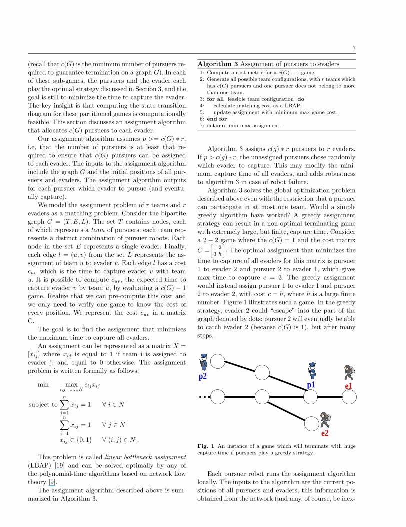
2 to evader 2, with cost c = h, where h is a large finitenumber. Figure 1 illustrates such a game. In the greedy

strategy, evader 2 could “escape” into the part of the

graph denoted by dots: pursuer 2 will eventually be ableto catch evader 2 (because c(G) is 1), but after many

steps.

e1 p1

e2

p2

Fig. 1 An instance of a game which will terminate with huge

capture time if pursuers play a greedy strategy.

Each pursuer robot runs the assignment algorithmlocally. The inputs to the algorithm are the current po-

sitions of all pursuers and evaders; this information is

obtained from the network (and may, of course, be inex-

8

act because of sensing noise). Each pursuer executes the

assignment only once, and sticks with the assignmentuntil the game terminates.

4.1 Complexity

The number of evaluated team configurations x can be

modelled as the number of ways to put p distinct balls

in r identical boxes. Each distinct ball represents a pur-suer and each identical box represents an evader. The

boxes are identical because we do not need to deter-

mine the identity of the evaders, the matching will de-termine this. For instance, if c(G) = 3, r = 2, p = 6,

configuration < p1p2p3 >< p4p5p6 > is equivalent to

< p4p5p6 >< p1p2p3 > in our matching input. More-

over, each box should have c(G) balls.The number of ways to put p distinct balls in r

identical boxes is to first imagine the boxes as distinct

and then determine what we over-counted. The numberof distributions of a set of p distinct balls into a set of r

distinct boxes if each box is to hold a specified number

of balls is(

pp1,p2,...,pr

)

= p!Q

ri=1 pi!

where p1+p2+...+pr =

p. In our case, since all pi = c(G), we have p!(c(G)!)r . Due

the fact that the boxes are identical, we over-counted

r!. Hence, the number of configuration x we have isx = p!

(c(G)!)r∗(r!) .

Given that n! ' nn (Stirling’s approximation), wehave x ' pp

(c(G))c(G)∗r∗(rr)

. If p = c(G) ∗ r, we have

the number of evaluated configuration x ' rp−r. Thecomplexity of the Linear Bottleneck Assignment Prob-

lem (LBAP) with N nodes is O(N 2) [32]. We eval-

uate x configurations, which has r nodes. Thus, the

complexity of this part of algorithm 3 is O(r2x). Wealso need to evaluate a c(G) − 1 game to know the

cost metric, which has complexity O(|V |2(c(G)+1)) (from

Section 3). Thus, our overall complexity is O(r2x +|V |2(c(G)+1)), where x = p!

(c(G)!)r∗(r!) ' rp−r instead of

previous O(|V |2(p+r)). Since r << |V |, this algorithm

is significantly more computationally efficient.

4.2 Properties

Here we enumerate the properties of the partition strat-

egy.

Termination: Lemma 1 guarantees game will ter-minate, assuming no robot fails.

Lemma 1 Algorithm 3 guarantees that the p− r game

will terminate.

Proof Since we decompose the p−r game into r parallel

c(G)−1 sub-games, and each of these games is guaran-

teed to terminate by Theorem 1, the overall p− r game

terminates.

Optimality of partitioning: Algorithm 3 opti-

mally partitions the evaders across the pursuers, sub-

ject to the cost metric. More precisely, there is no bet-

ter way in partition the game into c(G)-1 games. Thisproperty follows from the optimality of the LBAP as-

signment algorithm.

Bounded capture time: The completion time for

the p− r game is the maximum completion time across

the c(G)−1 sub-game. However, is it still an open ques-tion how far off from the optimal completion time this

partition strategy is.

Scalability: Algorithm 3 scales better than the op-timal strategy, since its scaling is dominate by rp−r,

while the optimal scales as |V |p+r, and usually r <<

|V |.

Robustness: If p > c(G)∗r, algorithm 3 can assign

extra pursuers to evaders to ensure robustness to robot

failures.

To summarize, algorithm 3 works as follows. In a de-

centralized manner, each robot pre-computes a c(G)−1state transition diagram. Then, after being informed by

the network of the positions of all robots, each robot

runs the assignment algorithm described above once.Thereafter, using the pre-computed state transition di-

agram and network localization updates, all robots con-

tinuously play the game until all evaders are captured.

5 Design

In this section, we discuss the hardware and networktestbed which form the basis for our pursuit-evasion

experiments. We then describe, in some detail, our PEG

software design and implementation. This sets the stagefor our system evaluation, which is discussed in the next

section.

5.1 Platform

The Robot Platform. We use a commoditized robotics

platform and made minimal modifications to it usingcommercial off-the-shelf products. Our platform con-

sists of an iRobot Create and a small embedded com-

puter mounted on top of it (Figure 2).

The Create, a differential drive robot, has a round

chassis of 33 cm diameter. The robot essentially has two

kinds of sensors. First, a pair of tactile sensors that, to-gether with a bumper, can help determine whether a

robot hits an obstacle and the angle at which it does

so. Second, a suite of infrared (IR) sensors: the bumper

9

contains an IR wall sensor on the right and an omnidi-

rectional IR receiver in the top, and four additional IRsensors mounted underneath the bumper facing down.

We do not add additional sensing hardware to the Cre-

ate.

The embedded computer, the Ebox 3854, is an 800

MHz embedded PC with 256MB shared DDR memory,

and supports a 1280x1024 VGA interface, one 10/100LAN, and USB, mini PCI and compact flash sockets.

The Ebox contains a 4GB compact flash (CF) card. Fi-

nally, we chose the EMP-8602 mini-PCI 802.11 a/b/g

wireless card to provide network connectivity. This choiceof platform is primarily designed to enable ease of pro-

gramming (the Ebox runs standard Linux), and has

enough ports to support various connectivity options.The embedded computer is powered by the Create’s

battery through a DC-DC power adapter (picoPSU).

The embedded computer is powered by the Create’sbattery. Since the two devices have incompatible volt-

age, we use a commercial DC-DC power adapter called

the picoPSU. To use the adapter we had to fabricate

custom connectors to the adapter, and to reconfigurethe pins on the adapter itself, the details of which are

beyond the scope of this paper.

The embedded computer runs Linux Fedora Core 6as the operating system. For sensing and control, we de-

veloped a Create driver for Player [13], using which we

are able to move the robot, turn on/off LEDs, read thebumpers, buttons and IR sensors. We set the nominal

speed to 0.2 m/s.

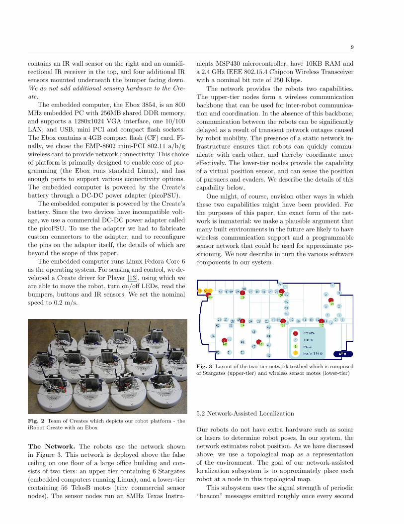
Fig. 2 Team of Creates which depicts our robot platform - the

iRobot Create with an Ebox

The Network. The robots use the network shown

in Figure 3. This network is deployed above the false

ceiling on one floor of a large office building and con-

sists of two tiers: an upper tier containing 6 Stargates(embedded computers running Linux), and a lower-tier

containing 56 TelosB motes (tiny commercial sensor

nodes). The sensor nodes run an 8MHz Texas Instru-

ments MSP430 microcontroller, have 10KB RAM and

a 2.4 GHz IEEE 802.15.4 Chipcon Wireless Transceiverwith a nominal bit rate of 250 Kbps.

The network provides the robots two capabilities.

The upper-tier nodes form a wireless communicationbackbone that can be used for inter-robot communica-

tion and coordination. In the absence of this backbone,

communication between the robots can be significantlydelayed as a result of transient network outages caused

by robot mobility. The presence of a static network in-

frastructure ensures that robots can quickly commu-

nicate with each other, and thereby coordinate moreeffectively. The lower-tier nodes provide the capability

of a virtual position sensor, and can sense the position

of pursuers and evaders. We describe the details of thiscapability below.

One might, of course, envision other ways in which

these two capabilities might have been provided. Forthe purposes of this paper, the exact form of the net-

work is immaterial: we make a plausible argument that

many built environments in the future are likely to have

wireless communication support and a programmablesensor network that could be used for approximate po-

sitioning. We now describe in turn the various software

components in our system.

Fig. 3 Layout of the two-tier network testbed which is composedof Stargates (upper-tier) and wireless sensor motes (lower-tier)

5.2 Network-Assisted Localization

Our robots do not have extra hardware such as sonar

or lasers to determine robot poses. In our system, thenetwork estimates robot position. As we have discussed

above, we use a topological map as a representation

of the environment. The goal of our network-assisted

localization subsystem is to approximately place eachrobot at a node in this topological map.

This subsystem uses the signal strength of periodic

“beacon” messages emitted roughly once every second

10

(we add some randomization to the interval to reduce

collisions) by the robots themselves.

The second-tier motes receive these beacons, and re-port all beacons whose signal strength is above a certain

threshold. Tenet [14], a readily available open-source

software package for programming wireless sensor net-works, is the software that collects the beacon signal

strength. A centralized robot location server then ap-

plies a voting scheme on a sliding window of reports (thewidth of the window is 7) to generate a location esti-

mate. Since radio propagation characteristics can vary

significantly even with small displacements, we use a

simple heuristic filter to smooth the estimate. This fil-ter essentially updates a robot’s current position only

after n consecutive reports are received. Clearly, this

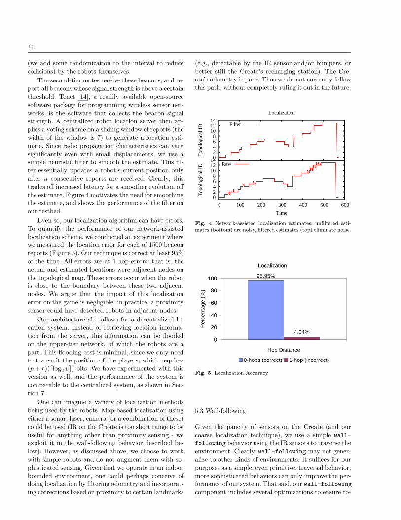
trades off increased latency for a smoother evolution offthe estimate. Figure 4 motivates the need for smoothing

the estimate, and shows the performance of the filter on

our testbed.

Even so, our localization algorithm can have errors.

To quantify the performance of our network-assistedlocalization scheme, we conducted an experiment where

we measured the location error for each of 1500 beacon

reports (Figure 5). Our technique is correct at least 95%of the time. All errors are at 1-hop errors: that is, the

actual and estimated locations were adjacent nodes on

the topological map. These errors occur when the robotis close to the boundary between these two adjacent

nodes. We argue that the impact of this localization

error on the game is negligible: in practice, a proximity

sensor could have detected robots in adjacent nodes.

Our architecture also allows for a decentralized lo-cation system. Instead of retrieving location informa-

tion from the server, this information can be flooded

on the upper-tier network, of which the robots are apart. This flooding cost is minimal, since we only need

to transmit the position of the players, which requires

(p + r)(dlog2 ve) bits. We have experimented with thisversion as well, and the performance of the system is

comparable to the centralized system, as shown in Sec-

tion 7.

One can imagine a variety of localization methods

being used by the robots. Map-based localization usingeither a sonar, laser, camera (or a combination of these)

could be used (IR on the Create is too short range to be

useful for anything other than proximity sensing - weexploit it in the wall-following behavior described be-

low). However, as discussed above, we choose to work

with simple robots and do not augment them with so-

phisticated sensing. Given that we operate in an indoorbounded environment, one could perhaps conceive of

doing localization by filtering odometry and incorporat-

ing corrections based on proximity to certain landmarks

(e.g., detectable by the IR sensor and/or bumpers, or

better still the Create’s recharging station). The Cre-ate’s odometry is poor. Thus we do not currently follow

this path, without completely ruling it out in the future.

0 2 4 6 8

10 12 14

0 100 200 300 400 500 600T

opol

ogic

al I

D

Time

Raw 0 2 4 6 8

10 12 14

Top

olog

ical

ID

Localization

Filter

Fig. 4 Network-assisted localization estimates: unfiltered esti-

mates (bottom) are noisy, filtered estimates (top) eliminate noise.

Localization

95.95%

4.04%0

20

40

60

80

100

Hop Distance

Per

cent

age

(%)

0-hops (correct) 1-hop (incorrect)

Fig. 5 Localization Accuracy

5.3 Wall-following

Given the paucity of sensors on the Create (and our

coarse localization technique), we use a simple wall-

following behavior using the IR sensors to traverse the

environment. Clearly, wall-following may not gener-

alize to other kinds of environments. It suffices for our

purposes as a simple, even primitive, traversal behavior;more sophisticated behaviors can only improve the per-

formance of our system. That said, our wall-following

component includes several optimizations to ensure ro-

11

bustness: in our environment, at least, it always results

in forward progress.The robot continuously emits IR signals and reads

the IR receiver continuously. As long as the IR values

are between two thresholds and none of the bumpersare activated, the robot will move forward parallel to

the wall using simple PD control.

If the IR reading falls below a threshold, the robotassumes it has “lost” the wall and attempts to search

for it. It does this by executing a spiral (simultane-

ous rotation and translation) until the bumper senses

contact (assumed to be with the wall). To avoid openoffice or elevator doors in the experiments, we use a

“virtual wall” (essentially, an IR transmitter) available

from iRobot. When the virtual wall is detected, therobot tries to avoid going through it by going back

and turning to the left for a while without bumping,

then going forward while turning to the right also with-out bumping. If the bump sensor is activated and the

virtual wall is simultaneously detected, it invokes the

escape behavior described below.

The escape behavior is invoked whenever the robotis stuck. In addition to the scenario discussed above,

this behavior is invoked whenever the power consump-

tion of the robot is above a predetermined thresholdover a predefined time window (this might happen when

the robot encounters a small obstacle that does not ac-

tivate the bumper). To execute the escape behavior, therobot simply moves backwards for a short distance and

then resumes wall-following.

Our robot’s wall following behavior uses the IR trans-

mitter near the right side of the robot. As such, it keepsthe wall to its right. To reverse direction, the robot im-

plements a detach behavior which enables it to cross

a corridor and find the opposite wall. The detach be-havior is simple: the robot swivels slightly to the left

and then moves in an arc until a bumper is activated.

However, if the robot hits a wall in less than a presettime, it repeats this maneuver since it is unlikely to

have crossed the corridor in that (short) time.

5.4 Navigation

The navigation component calculates the goal position,

and invokes wall-following to move from one topo-

logical node to the adjacent one. Navigation is executedevery time the robot changes its position (as well as

when any evader changes its position), so the robot con-

tinuously updates its trajectory.

The navigation component calculates the goal posi-tion given its team’s position and that of its assigned

evader. Using Algorithm 1, we pre-compute a state tran-

sition diagram for a given team configuration. This state

transition diagram is pre-loaded on all the robots, and

each pursuer or evader makes a decentralized local statetransition decision, given the current state. This deci-

sion tells the robot which topological node to move to

next.

However, there exists an important subtlety in thenavigation algorithm imposed by the minimality of our

platform. Our robot has no inherent proprioception ca-

pability, it can only travel parallel to a wall, keeping

the wall to its right (since the robot has only one IRwall sensor positioned on its right). As a result, the

robot might actually move in a direction opposite to

that intended by the navigation component. To rectifythis, we add a simple a posteriori correction to the nav-

igation component. If the wall-following moves the

robot to a node that it does not expect to arrive at, itinvokes the detach behavior described above to reverse

direction.

6 Simulation

In this section, we evaluate the optimal and partition

strategy by simulation. We implemented an idealizedgame simulator, which models time in discrete steps and

implements the strategy discussed in Section 3.1. We

exhaustively enumerate all configurations to compute a

worst-case configuration.

6.1 Optimal Strategy

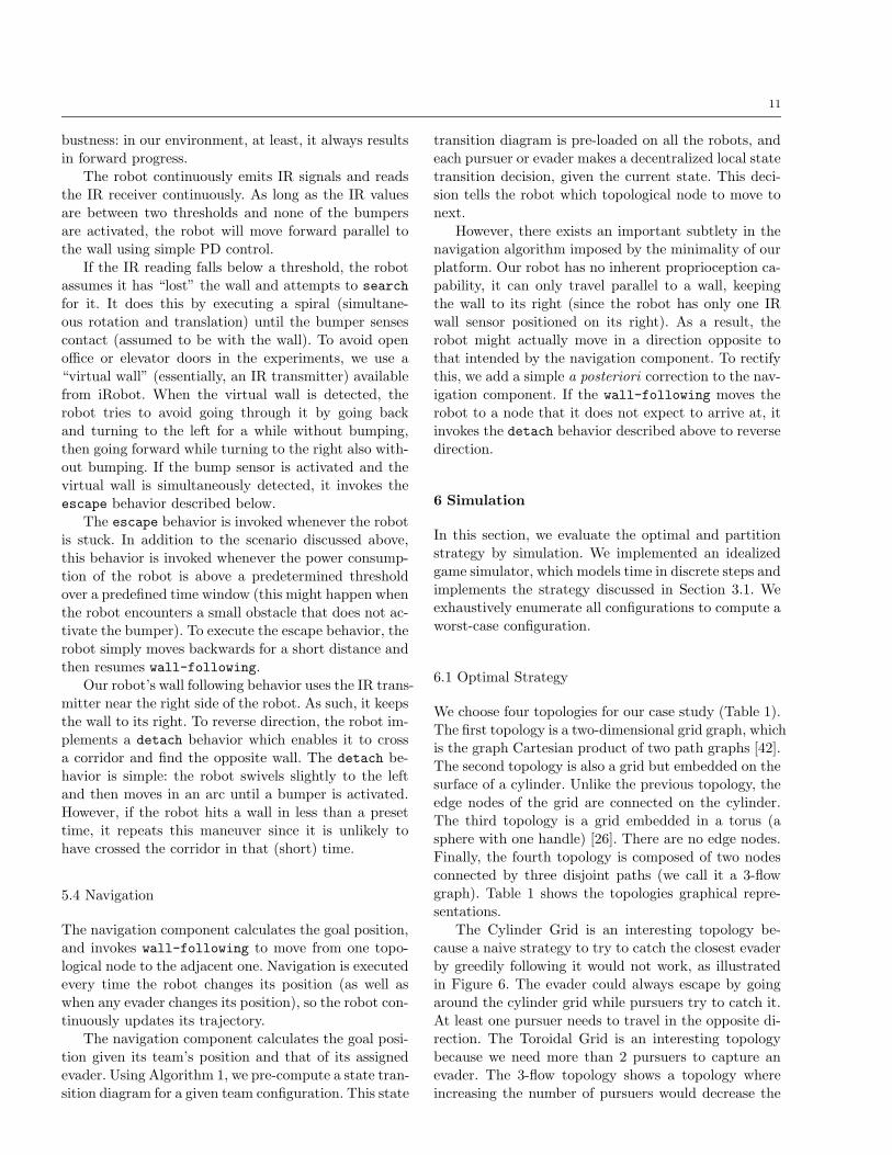
We choose four topologies for our case study (Table 1).

The first topology is a two-dimensional grid graph, which

is the graph Cartesian product of two path graphs [42].

The second topology is also a grid but embedded on thesurface of a cylinder. Unlike the previous topology, the

edge nodes of the grid are connected on the cylinder.

The third topology is a grid embedded in a torus (asphere with one handle) [26]. There are no edge nodes.

Finally, the fourth topology is composed of two nodes

connected by three disjoint paths (we call it a 3-flowgraph). Table 1 shows the topologies graphical repre-

sentations.

The Cylinder Grid is an interesting topology be-

cause a naive strategy to try to catch the closest evader

by greedily following it would not work, as illustratedin Figure 6. The evader could always escape by going

around the cylinder grid while pursuers try to catch it.

At least one pursuer needs to travel in the opposite di-

rection. The Toroidal Grid is an interesting topologybecause we need more than 2 pursuers to capture an

evader. The 3-flow topology shows a topology where

increasing the number of pursuers would decrease the

12

Topology Name Graphical Game C(G) 2 pursuers 3 pursuers

Grid 2D 4x4

2

3

5

1

4

2

3 4

2

5

3 4

5

6

1 1

6

2 6 6

Cylinder Grid 4x4

1

2

3 4

1

2

3

4 5

1

2

3

4 5 5

2 5 5

Toroidal Grid 4x4

1 2 2

3 3

1

1 2 3 3

4

4

2

2

3 4

1

2 3 4

3 ∞ 4

3-flow N/A 2 3 1

2

2

3

3 1

1

2 4 3

Table 1 Instances of Games and their properties

worst-case capture time. The 3-flow topology needs only2 pursuers to guarantee the capture of an evader. But,

with 3 pursuers, the worst-case capture time decreases

from 4 to 3 steps.

Table 1 shows some instances of games and theirproperties. The third column illustrates a worst-case

capture game on the given topology. The game shows

the trajectory of each player. The nodes and solid undi-

rected edges connecting them represent the topologi-cal map. The solid directed lines (lines with arrows)

show the pursuer path and the dashed lines illustrate

the evader path. The edge labels represent the time se-

quence of the robots. The pursuer and evader’s initialpositions are indicated by the corresponding icons. The

fourth column is the necessary number of pursuers to

guarantee the termination of the game. The fifth and

13

Fig. 6 A game where pursuer greedily follow the evader will not

terminate in a cylinder Grid Topology.

sixth columns represent the maximum number of steps

to terminate the game, given the number of pursuers.

It is interesting to see that even though the torus needsat least 3 pursuers, if we play the game with 3 pursuers,

the game will be shorter than in a 4x4 grid. Another

interesting fact is increasing the number of edges fromgrid 2d 4x4 to cylinder 4x4 does not increase the nec-

essary number of pursuers but it decreases the number

of steps to terminate the game. Increasing the edgesagain (from cylinder to toroidal), increases the neces-

sary number of pursuers.

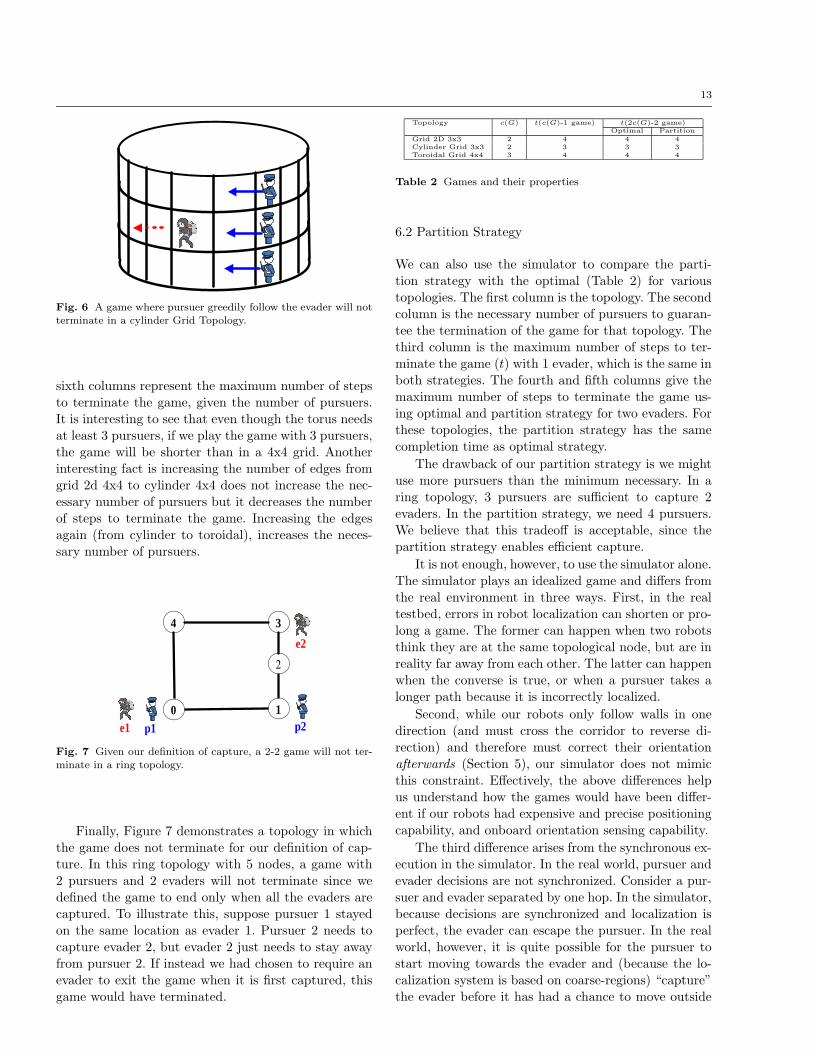
2

3 4

e2

e1 0

p1 p2 1

Fig. 7 Given our definition of capture, a 2-2 game will not ter-

minate in a ring topology.

Finally, Figure 7 demonstrates a topology in whichthe game does not terminate for our definition of cap-

ture. In this ring topology with 5 nodes, a game with

2 pursuers and 2 evaders will not terminate since wedefined the game to end only when all the evaders are

captured. To illustrate this, suppose pursuer 1 stayed

on the same location as evader 1. Pursuer 2 needs to

capture evader 2, but evader 2 just needs to stay awayfrom pursuer 2. If instead we had chosen to require an

evader to exit the game when it is first captured, this

game would have terminated.

Topology c(G) t(c(G)-1 game) t(2c(G)-2 game)Optimal Partition

Grid 2D 3x3 2 4 4 4Cylinder Grid 3x3 2 3 3 3Toroidal Grid 4x4 3 4 4 4

Table 2 Games and their properties

6.2 Partition Strategy

We can also use the simulator to compare the parti-

tion strategy with the optimal (Table 2) for varioustopologies. The first column is the topology. The second

column is the necessary number of pursuers to guaran-

tee the termination of the game for that topology. Thethird column is the maximum number of steps to ter-

minate the game (t) with 1 evader, which is the same in

both strategies. The fourth and fifth columns give the

maximum number of steps to terminate the game us-ing optimal and partition strategy for two evaders. For

these topologies, the partition strategy has the same

completion time as optimal strategy.

The drawback of our partition strategy is we might

use more pursuers than the minimum necessary. In a

ring topology, 3 pursuers are sufficient to capture 2evaders. In the partition strategy, we need 4 pursuers.

We believe that this tradeoff is acceptable, since the

partition strategy enables efficient capture.

It is not enough, however, to use the simulator alone.The simulator plays an idealized game and differs from

the real environment in three ways. First, in the real

testbed, errors in robot localization can shorten or pro-long a game. The former can happen when two robots

think they are at the same topological node, but are in

reality far away from each other. The latter can happenwhen the converse is true, or when a pursuer takes a

longer path because it is incorrectly localized.

Second, while our robots only follow walls in onedirection (and must cross the corridor to reverse di-

rection) and therefore must correct their orientation

afterwards (Section 5), our simulator does not mimic

this constraint. Effectively, the above differences helpus understand how the games would have been differ-

ent if our robots had expensive and precise positioning

capability, and onboard orientation sensing capability.

The third difference arises from the synchronous ex-

ecution in the simulator. In the real world, pursuer and

evader decisions are not synchronized. Consider a pur-suer and evader separated by one hop. In the simulator,

because decisions are synchronized and localization is

perfect, the evader can escape the pursuer. In the real

world, however, it is quite possible for the pursuer tostart moving towards the evader and (because the lo-

calization system is based on coarse-regions) “capture”

the evader before it has had a chance to move outside

14

the region. In these infrequent cases, the game can ter-

minate faster than it would in the idealized scenario.

For this reason, we played a few (specifically, 2− 1,

4 − 2, and 6− 3) games on our real world testbed, and

we discuss the results below.

7 Experiments

In this section, we describe the results from severalgames played on the physical robot testbed described

in Section 5.

We play the games on the floor plan shown in Fig-ure 3, using the network whose nodes are shown in that

figure. We run the experiments in the entire floorplan,

which has about 50 m x 30m, providing us a realis-

tic physical large environment. While our games areplayed only in the one environment shown (and future

work needs to validate the generality of the claims we

make later in this section), we emphasize two importantpoints about the environment that lead us to believe

that our results would hold generally in other similar

environments. First, our building floor is representa-tive of many office buildings (i.e., it does not have any

unusual features that would materially affect our con-

clusions) and we do not alter the environment in any

way other than to place virtual walls in some locations2.Second, our network design is not optimized in any way

for this particular application. Rather, the network was

designed to mimic harsh wireless communication con-ditions to stress test wireless systems and applications.

0

0.2

0.4

0.6

0.8

1

0 50 100 150 200 250

Frac

tion

of R

epor

ts

Latency (ms)

Latency

Fig. 8 The communication latency for detecting the robots.

2 We place a virtual wall in front of the elevator doors to pre-

vent the robot from entering an open elevator. We also place a

virtual wall in front of the doors whose thresholds are lower than

the height of the Create bumper.

Figure 8 shows the cumulative latency for beacon re-

ports from robots. The latency measures the time fromwhen the robot sends a beacon to when the robot lo-

cation server receives it. This communication latency

is at most 250 ms. We expect the latency of distribut-ing the location estimate to the robots from the server

to be comparable. Thus, our real-world implementation

deviates from our simulations and theory in that robotposes may be slightly stale: however, given the robot

speeds in our experiments, the location estimates will

be off by about 0.1 m or so, a relatively small amount.

The convergence time of a game depends on theinitial configuration. We play our games using a worst-

case initial configuration (there can be many), which

was calculated by the idealized game simulator.

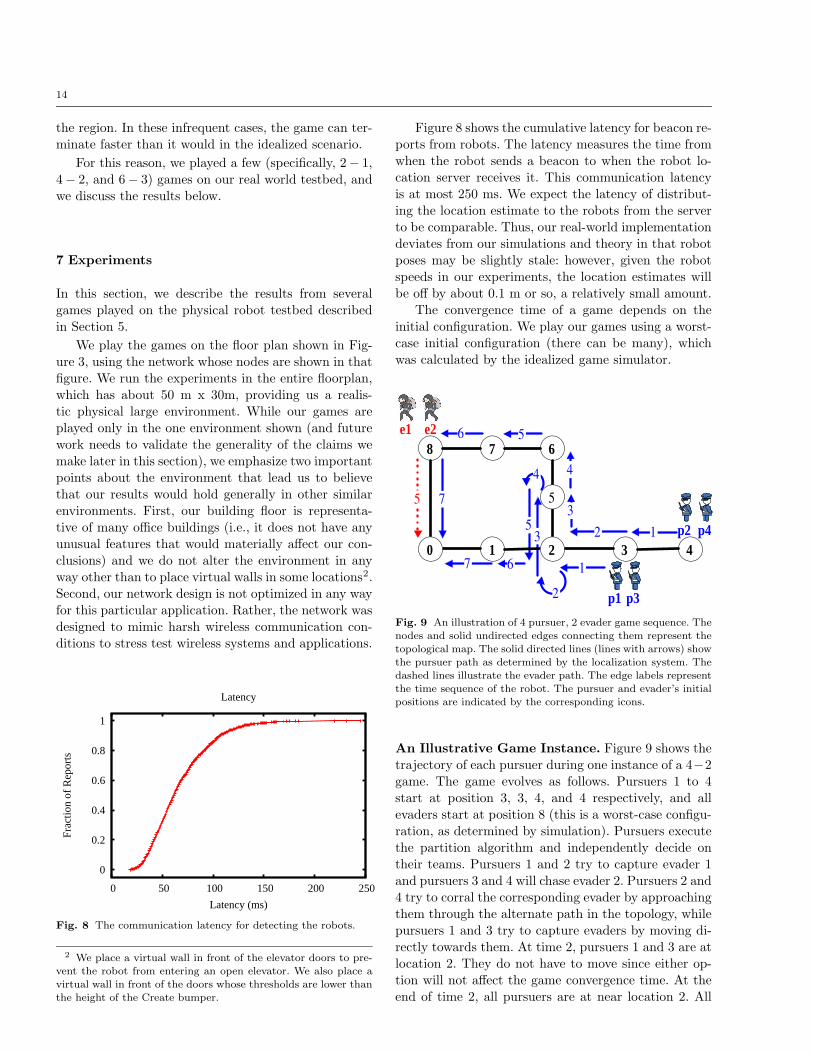
1 3 4

6 7 8 4

2 3

5 6 e1

p1 p3

p4

e2

0 1

6 7

3 5

2

5

p2

1 2

4 7 5

Fig. 9 An illustration of 4 pursuer, 2 evader game sequence. The

nodes and solid undirected edges connecting them represent thetopological map. The solid directed lines (lines with arrows) showthe pursuer path as determined by the localization system. The

dashed lines illustrate the evader path. The edge labels representthe time sequence of the robot. The pursuer and evader’s initial

positions are indicated by the corresponding icons.

An Illustrative Game Instance. Figure 9 shows the

trajectory of each pursuer during one instance of a 4−2

game. The game evolves as follows. Pursuers 1 to 4start at position 3, 3, 4, and 4 respectively, and all

evaders start at position 8 (this is a worst-case configu-

ration, as determined by simulation). Pursuers executethe partition algorithm and independently decide on

their teams. Pursuers 1 and 2 try to capture evader 1

and pursuers 3 and 4 will chase evader 2. Pursuers 2 and4 try to corral the corresponding evader by approaching

them through the alternate path in the topology, while

pursuers 1 and 3 try to capture evaders by moving di-

rectly towards them. At time 2, pursuers 1 and 3 are atlocation 2. They do not have to move since either op-

tion will not affect the game convergence time. At the

end of time 2, all pursuers are at near location 2. All

15

0100200300400500600700

2-1 4-2 6-3Game Configuration (#Pursuers-#Evaders)

Mea

nC

aptu

reT

ime

(s)

Centralized Location UpdatesDistributed Location UpdatesSimulation

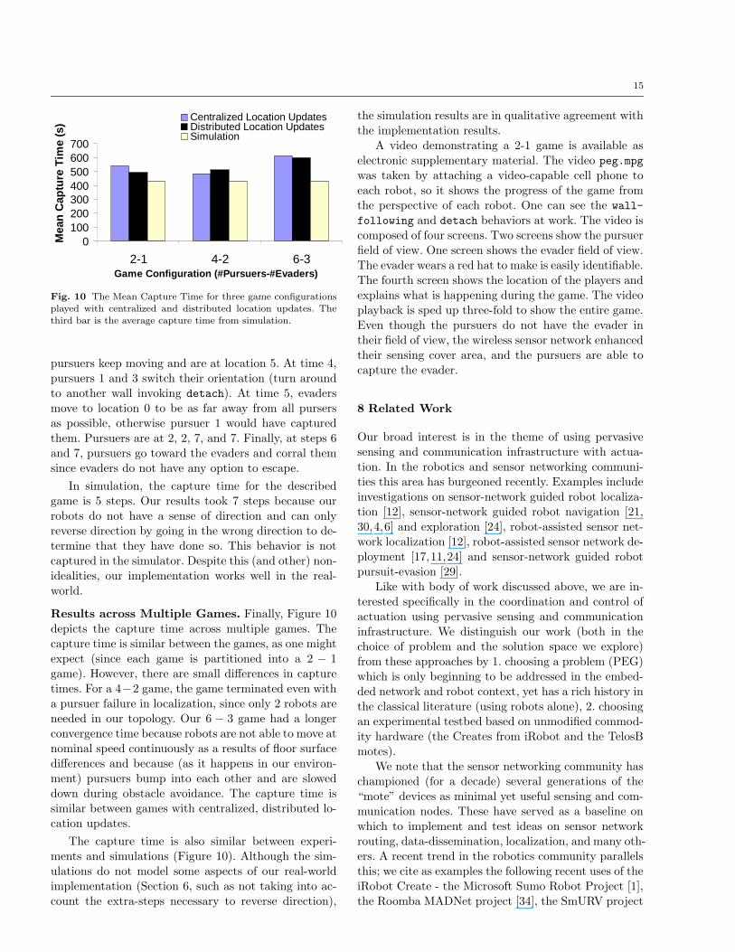
Fig. 10 The Mean Capture Time for three game configurations

played with centralized and distributed location updates. The

third bar is the average capture time from simulation.

pursuers keep moving and are at location 5. At time 4,pursuers 1 and 3 switch their orientation (turn around

to another wall invoking detach). At time 5, evaders

move to location 0 to be as far away from all pursersas possible, otherwise pursuer 1 would have captured

them. Pursuers are at 2, 2, 7, and 7. Finally, at steps 6

and 7, pursuers go toward the evaders and corral them

since evaders do not have any option to escape.

In simulation, the capture time for the describedgame is 5 steps. Our results took 7 steps because our

robots do not have a sense of direction and can only

reverse direction by going in the wrong direction to de-termine that they have done so. This behavior is not

captured in the simulator. Despite this (and other) non-

idealities, our implementation works well in the real-world.

Results across Multiple Games. Finally, Figure 10

depicts the capture time across multiple games. Thecapture time is similar between the games, as one might

expect (since each game is partitioned into a 2 − 1

game). However, there are small differences in capture

times. For a 4−2 game, the game terminated even witha pursuer failure in localization, since only 2 robots are

needed in our topology. Our 6 − 3 game had a longer

convergence time because robots are not able to move atnominal speed continuously as a results of floor surface

differences and because (as it happens in our environ-

ment) pursuers bump into each other and are sloweddown during obstacle avoidance. The capture time is

similar between games with centralized, distributed lo-

cation updates.

The capture time is also similar between experi-

ments and simulations (Figure 10). Although the sim-ulations do not model some aspects of our real-world

implementation (Section 6, such as not taking into ac-

count the extra-steps necessary to reverse direction),

the simulation results are in qualitative agreement with

the implementation results.A video demonstrating a 2-1 game is available as

electronic supplementary material. The video peg.mpg

was taken by attaching a video-capable cell phone toeach robot, so it shows the progress of the game from

the perspective of each robot. One can see the wall-

following and detach behaviors at work. The video iscomposed of four screens. Two screens show the pursuer

field of view. One screen shows the evader field of view.

The evader wears a red hat to make is easily identifiable.

The fourth screen shows the location of the players andexplains what is happening during the game. The video

playback is sped up three-fold to show the entire game.

Even though the pursuers do not have the evader intheir field of view, the wireless sensor network enhanced

their sensing cover area, and the pursuers are able to

capture the evader.

8 Related Work

Our broad interest is in the theme of using pervasive

sensing and communication infrastructure with actua-tion. In the robotics and sensor networking communi-

ties this area has burgeoned recently. Examples include

investigations on sensor-network guided robot localiza-tion [12], sensor-network guided robot navigation [21,

30,4,6] and exploration [24], robot-assisted sensor net-

work localization [12], robot-assisted sensor network de-

ployment [17,11,24] and sensor-network guided robotpursuit-evasion [29].

Like with body of work discussed above, we are in-

terested specifically in the coordination and control ofactuation using pervasive sensing and communication

infrastructure. We distinguish our work (both in the

choice of problem and the solution space we explore)from these approaches by 1. choosing a problem (PEG)

which is only beginning to be addressed in the embed-

ded network and robot context, yet has a rich history in

the classical literature (using robots alone), 2. choosingan experimental testbed based on unmodified commod-

ity hardware (the Creates from iRobot and the TelosB

motes).We note that the sensor networking community has

championed (for a decade) several generations of the

“mote” devices as minimal yet useful sensing and com-munication nodes. These have served as a baseline on

which to implement and test ideas on sensor network

routing, data-dissemination, localization, and many oth-

ers. A recent trend in the robotics community parallelsthis; we cite as examples the following recent uses of the

iRobot Create - the Microsoft Sumo Robot Project [1],

the Roomba MADNet project [34], the SmURV project

16

[38] [3] [37] [16] [18] [39] [29] Our work

Pursuer to Evader Ratio ≥ 1 ≥ 1 1 ≥ 1 ≥ 1 ≥ 1 1 � 1

Pursuer Visibility full full full local local local full full

Evader Visibility full full full full full local none full

Information full full full full full no pursuer full full

Environment Graph Graph Polygon Polygon Polygon Polygon Polygon Graph

Capture touch touch touch see touch touch touch touch

Speed (faster entity) any same same same evader any same any

Time to Capture yes no no no no no no yes

Robot Implementation None None None None None Partial Partial Full

Table 3 Related Work in Pursuit-Evasion

[2], and the workbook associated with a recent text on

robotics [23].

To situate our work in the existing literature, weclassify the type of PEGs using seven criteria: the ratio

of the number of pursuers to the number of evaders;

whether pursuers and evaders have full and/or global

visibility, or whether they can only see within a thresh-old distance or until occluded by an obstacle (usually

modelled by the edge of a polygon in 2D); what ad-

ditional information robots have with respect to theopponents’ strategy or planning algorithm; whether the

environment is modelled as a graph (discrete) or a poly-

gon (continuous half-space with lines in 2D as bound-aries); how the evader is captured, whether by being sur-

rounded, seen or sensed by the pursuer, or approached

within a certain distance, or physically contacted; the

relative speed between the pursuer and evader;and, ifthe time to capture is important.

Table 3 shows a classification of the related work

in the literature along these dimensions. Our work isdistinct from several pieces of prior work. Its novelty

is clear in several dimensions: while other work has ex-

plored theoretical bounds on eventual capture [3,37], orpursuit-evasion under constrained geometries [16,25,8,

10], or has examined sophisticated control strategies [39,

29], our proposed work attempts to minimize the time

of capture of a multi-pursuer multi-evader under thepragmatic realization of physical multi-robot games.

Complementary to our work, [38] discusses a dy-

namic programming algorithm to maintain connectiv-ity in a team of robotic routers in the case where there

is one user moving in an adversarial trajectory. The

problem is modeled as a pursuit-evasion game, with thegoal of finding the shortest escape trajectory. There is

no discussion on how to initially detect the evader. The

algorithm has complexity O(v3(p+1)). They presentedsimulation results and were seeking an improved run-

ning time.

In [7], an algorithm to determine if K pursuers are

sufficient to capture an evader is presented. They alsoshowed that every graph is topologically equivalent to

a graph with pursuer number at most two. In the sur-

vey presented by Alspach [5], a number of references

on the necessary number of pursuers for a given graph

class can be found. Aigner and Fromme [3] proved that

in a planar graph G, 3 pursuers are sufficient for the

pursuers to win the game. Quilliot [33] extended thisresult, giving an upper bound to the number of pur-

suers depending on the genus of the graph G. In [27],

the necessary number of pursuers is studied under threegraph product operations. In [15], given certain condi-

tions, the complexity of pursuit on a graph is Exptime-

complete.

For superior evaders, Seymour [36] showed that find-ing the necessary number of pursuers to capture a single

evader with infinite velocity in a graph G when pur-

suers and evader move simultaneously is equivalent to

finding the treewidth of G. Other works [41][40] focuson an Euclidean open plane and provide sub-optimal

real-time approaches.

We are the first to present a scalable algorithm to

minimize the time to capture of a multi-pursuer multi-evader game, and to validate the complete system in a

real-world implementation.

9 Conclusions

In this paper, we have described a system that detects

multiple evaders using wireless sensor network, dissem-

inates the necessary information using a decentralized

protocol, and executes an algorithm that captures mul-tiple evaders in near-optimal capture time. We have

presented a systematic derivation of this algorithm, by

first presenting a provably optimal algorithm capturesthe evaders in the minimum capture time, when the

evaders and pursuers are equipotent and play optimally.

We have then described an optimal algorithm for thesuperior evader case. Our third practical algorithm, is

an assignment algorithm that guarantees the game ter-

minates, has bounded captured time, is robust, and is

scalable in the number of robots. We have validated thefeasibility of our algorithm by experimentally playing

mobile robot-based pursuit evasion games on a physi-

cal testbed.

17

References

1. Sumo Robot (2008). URL http://msdn2.microsoft.com/en-

us/robotics/bb403184.aspx2. The SmURV Robotics Platform (2008)3. Aigner. M, F.M.: A Game of Cops and Robber. Tech. rep.

(1984)4. Alankus, G., Atay, N., Lu, C., Bayazit, B.: Adaptive Embed-

ded Roadmaps for Sensor Networks. In: IEEE International

Conference on Robotics and Automation (2007)5. Alspach, B.: Searching and Sweeping Graphs: a Brief Survey.

Le Matematiche (Catania) 59, 5–37 (2004)6. Batalin, M.A., Sukhatme, G.S.: Coverage, Exploration and

Deployment by a Mobile Robot and Communication Net-

work. In: Telecommunication Systems Journal, Special Issue

on Wireless Sensor Networks, pp. 376–391 (2003)7. Berarducci, A., Intrigila, B.: On the Cop Number of a

Graph. Adv. Appl. Math. 14(4), 389–403 (1993). DOI

http://dx.doi.org/10.1006/aama.1993.10198. Bhattacharya, S., Candido, S., Hutchinson, S.: Motion

Strategies for Surveillance. In: Robotics: Science and Sys-tems (2007)

9. Burkard, R.E., Cela, E.: Linear Assignment Problems andExtensions. Handbook of Combinatorial Optimization 4

(1999)10. Cheung, W.: Constrained Pursuit-Evasion Problems in the

Plane. Master Thesis, U.British Columbia (2005)11. Corke, P.I., Hrabar, S.E., Peterson, R., Rus, D., Saripalli, S.,

Sukhatme, G.S.: Deployment and Connectivity Repair of aSensor Net. In: 9th International Symposium on Experimen-

tal Robotics 2004 (2004)12. Corker, P., Peterson, R., Rus, D.: Localization and Naviga-

tion Assisted by Networked Cooperating Sensors and Robots.International Journal of Robotics Research 24(9), 771–786

(2005)13. Gerkey, B.P., Vaughan, R.T., Støy, K., Howard, A.,

Sukhatme, G.S., Mataric, M.J.: Most Valuable Player: a

Robot Device Server for Distributed Control. pp. 1226–1231.Maui, HI, USA (2001)

14. Gnawali, O., Greenstein, B., Jang, K.Y., Joki, A., Paek, J.,

Vieira, M., Estrin, D., Govindan, R., Kohler, E.: The TENETArchitecture for Tiered Sensor Networks. In: Proceedings ofthe ACM Conference on Embedded Networked Sensor Sys-

tems (2006)15. Goldstein, A.S., Reingold, E.M.: The Complexity of Pursuit

on a Graph. Theor. Comput. Sci. 143(1), 93–112 (1995).DOI http://dx.doi.org/10.1016/0304-3975(95)80012-3

16. Guibas, L.J., Latombe, J.C., LaValle, S.M., Lin, D., Mot-

wani, R.: Visibility-Based Pursuit-Evasion in a Polygonal

Environment. In: WADS ’97: Proceedings of the 5th Inter-

national Workshop on Algorithms and Data Structures, pp.17–30. Springer-Verlag, London, UK (1997)

17. Howard, A., Mataric, M.J., Sukhatme, G.S.: An Incremen-

tal Self-Deployment Algorithm for Mobile Sensor Networks.

Autonomous Robots 13(2), 113–126 (2002)18. Isler, V., Kannan, S., Khanna, S.: Randomized Pursuit-

Evasion in a Polygonal Environment. IEEE Transactions

on Robotics 5(21), 864–875 (2005)19. Jonker, R., Volgenant, A.: A Shortest Augmenting Path

Algorithm for Dense and Sparse Linear Assignment Prob-

lems. Computing 38(4), 325–340 (1987). DOI

http://dx.doi.org/10.1007/BF0227871020. Kuipers, B., Byun, Y.T.: A Robot Exploration and Mapping

Strategy Based on a Semantic Hierarchy of Spatial Repre-

sentations. Tech. Rep. AI90-120 (1990)21. Li, Q., Rus, D.: Navigation Protocols in Sensor Networks.

ACM Tansactions on Sensor Networks 1(1), 3–35 (2005)

22. Mataric, M.J.: Integration of Representation Into Goal-

Driven Behavior-Based Robots. IEEE Transactions on

Robotics and Automation (3) (1992)

23. Mataric, M.J.: The Robotics Primer. MIT Press (2007)

24. Maxim Batalin and Gaurav S. Sukhatme: The Design and

Analysis of an Efficient Local Algorithm for Coverage and

Exploration Based on Sensor Network Deployment. IEEE

Transactions on Robotics 23(4), 661–675 (2007)

25. Murrieta-Cid, R., Muppirala, T., Sarmiento, A., Bhat-

tacharya, S., Hutchinson, S.: Surveillance Strate-

gies for a Pursuer with Finite Sensor Range.

Int. J. Rob. Res. 26(3), 233–253 (2007). DOI

http://dx.doi.org/10.1177/0278364907077083

26. Neufeld, E., Myrvold, W.: Practical Toroidality Testing. In:

SODA ’97: Proceedings of the Eighth Annual ACM-SIAM

Symposium on Discrete Algorithms, pp. 574–580. Society for

Industrial and Applied Mathematics, Philadelphia, PA, USA

(1997)

27. Neufeld, S., Nowakowski, R.: A Game of Cops and Rob-

bers Played on Products of Graphs. Discrete Math.186(1-3) (1998). DOI http://dx.doi.org/10.1016/S0012-365X(97)00165-9

28. Nowakowski, R.J., Winkler, P.: Vertex-to-Vertex Pursuit ina Graph. Discrete Mathematics 43(2-3), 235–239 (1983)

29. Oh, S., Schenato, L., Chen, P., Sastry, S.: Tracking and Coor-dination of Multiple Agents using Sensor Networks: SystemDesign, Algorithms and Experiments. Proceedings of theIEEE 95(1) (2007)

30. O’Hara, K.J., Bigio, V., Dodson, E., Irani, A., Walker, D.,Balch, T.: Physical Path Planning Using the Gnats. In:

IEEE International Conference on Robotics and Automation(2005)

31. Parsons, T.D.: Pursuit-Evasion in a Graph. LectureNotes in Mathematics 642, 426–441 (1978). DOI

10.1007/BFb0070400

32. Pferschy, U.: Solution Methods and Computational In-

vestigations for the Linear Bottleneck Assignment Prob-lem. Computing 59(3), 237–258 (1997). DOI

http://dx.doi.org/10.1007/BF02684443

33. Quilliot, A.: A Short Note About Pursuit Games Played on aGraph with a Given Genus. J. Comb. Theory, Ser. B 38(1),89–92 (1985)

34. Reich, J., Misra, V., Rubenstein, D.: Roomba MADNeT: aMobile Ad-hoc Delay Tolerant Network Testbed. In: MC2R:

Mobile Computing and Communications Review. ACM Sig-

mobile (2008)

35. Russell, S.J., Norvig, P.: Artificial Intelligence: A Modern

Approach. Pearson Education (2003)

36. Seymour, P.D., Thomas, R.: Graph Searching

and a Min-Max Theorem for Tree-Width. J.Comb. Theory Ser. B 58(1), 22–33 (1993). DOI

http://dx.doi.org/10.1006/jctb.1993.1027

37. Sgall, J.: Solution of David Gale’s Lion and Man Problem.

Theor. Comput. Sci. 259(1-2), 663–670 (2001)

38. Tekdas, O., Isler, V.: Robotic Routers. In: Proc. IEEE

Int. Conf. on Robotics and Automation (2008). URLhttp://www.cs.rpi.edu/. To appear

39. Vidal, R., Shakernia, O., Kim, H.J., Shim, D.H., Sastry, S.:

Probabilistic Pursuit-Evasion Games: Theory, Implementa-tion, and Experimental Evaluation. Robotics and Automa-

tion, IEEE Transactions on 18(5), 662–669 (2002)

40. Wang, X., Jose B. Cruz, J., Chen, G., Pham, K.,

Blasch, E.: Formation Control in Multi-Player Pur-suit Evasion Game with Superior Evaders. p.

657811. SPIE (2007). DOI 10.1117/12.723300. URL

http://link.aip.org/link/?PSI/6578/657811/1

18

41. Wei, M., Chen, G., Cruz, J., Hayes, L., Chang, M.H.: A De-

centralized Approach to Pursuer-Evader Games with Mul-

tiple Superior Evaders. Intelligent Transportation Systems

Conference, 2006. ITSC ’06. IEEE pp. 1586–1591 (2006).

DOI 10.1109/ITSC.2006.1707450

42. Weisstein, E.W.: Grid graph. MathWorld – A Wolfram Web

Resource. http://mathworld.wolfram.com/GridGraph.html.

URL http://mathworld.wolfram.com/GridGraph.html