lable at ScienceDirect

Journal of Environmental Management 133 (2014) 214e221

Contents lists avai

Journal of Environmental Management

journal homepage: www.elsevier .com/locate/ jenvman

Sediment and total phosphorous contributors in Rock River watershed

Eric G. Mbonimpa, Yongping Yuan*, Maliha S. Nash, Megan H. MehaffeyUSEPA Office of Research and Development, Landscape Ecology Branch, Las Vegas, USA

a r t i c l e i n f o

Article history:Received 21 February 2013Received in revised form12 November 2013Accepted 18 November 2013Available online

Keywords:Land usePLSRock River watershedTPTSS

* Corresponding author. Tel.: þ1 7027982112; fax:E-mail address: yuan.yongping@epa.gov (Y. Yuan)

0301-4797/$ e see front matter Published by Elseviehttp://dx.doi.org/10.1016/j.jenvman.2013.11.030

a b s t r a c t

Total phosphorous (TP) and total suspended sediment (TSS) pollution is a problem in the US Midwest andis of particular concern in the Great Lakes region where many water bodies are already eutrophic. In-creases in monoculture corn planting to feed ethanol based biofuel production could exacerbate thesealready stressed water bodies. In this study we expand on the previous studies relating landscape var-iables such as land cover, soil type and slope with changes in pollutant concentrations and loading in theGreat Lakes region.

The Rock River watershed in Wisconsin, USA was chosen due to its diverse land use, numerous lakesand reservoirs susceptible to TSS and TP pollution, and the availability of long-term streamflow, TSS andTP data. Eight independent subwatersheds in the Rock River watershed were identified using UnitedStates Geological Survey (USGS) monitoring sites that monitor flow, TSS and TP. For each subwatershed,we calculated land use, soil type, and terrain slope metrics or variables. TSS and TP from the differentsubwatersheds were compared using Analysis of Variance (ANOVA), and associations and relationshipsbetween landscape metrics and water quality (TSS and TP) were evaluated using the partial least square(PLS) regression. Results show that urban land use and agricultural land growing corn rotated with non-leguminous crops are associated with TSS and TP in streams. This indicates that increasing the amount ofcorn rotated with non-leguminous crops within a subwatershed could increase degradation of waterquality. Results showed that increase in cornesoybean rotation acreage within the watershed is asso-ciated with reduction in stream’s TSS and TP. Results also show that forest and water bodies wereassociated with reduction in TSS and TP. Based on our results we recommend adoption of the Low ImpactDevelopment (LID) approach in urban dominated subwatersheds. This approach attempts to replicate thepre-development hydrological regime by reducing the ratio of impervious area to natural cover whereverpossible, as well as recycling or treating stormwater runoff using filter strips, ponds and wetlands. Inagriculturally dominated subwatersheds, we recommend increasing cornesoybean rotation, keepingcorn on areas with gentle slope and soils with lower erodibility.

Published by Elsevier Ltd.

1. Introduction

Water bodies around the world are threatened by increases inupstream nutrients and sediment runoff as they influence sourcesof drinking water, aquatic species, and other ecologic functions ofstreams and lakes (Haycock and Muscutt, 1995; Verhoeven et al.,2006). Phosphorus, a primary nutrient, and sediment accelerateeutrophication and increase turbidity in water bodies. They couldoriginate from anthropogenic activities such as agriculture, urbandwelling, cattle, natural decay of organic matter and naturalerosion (Tong and Chen, 2002). The recent US policy to increasegeneration of ethanol biofuels from 13 billion gallons (bgals) in2010 to 36 bgals in 2022 (Congress, 2007; Schnepf, 2011) could

þ1 702 798 2208..

r Ltd.

cause an environmental challenge due to the potential loss ofconservation reserve program lands and cornesoybean rotations tomonoculture corn to meet the demands of energy. The majority ofthese agricultural-based biofuels are mainly generated from corngrown in US Midwest (Simpson et al., 2008).

Watershed scale studies on the potential effect of land usechanges will have on water quality are essential to controllingwater pollution. Various studies have linked stream pollutants toland use variables using process-based hydrological models (Jhaet al., 2010; Kirsch et al., 2002; Ullrich and Volk, 2009) or statisti-cal methods (Lenat and Crawford,1994; Liu et al., 2009; Lopez et al.,2008; Mehaffey et al., 2005; Nash et al., 2009). Process based hy-drologic models have been successfully used to characterizewatershed processes and sources of stream pollutants; howeverthese models require detailed input data, which may not be avail-able for some areas. For instance, Kirsch et al. (2002) showed thedifficulty of calibrating a SWAT model for Rock River basin in

E.G. Mbonimpa et al. / Journal of Environmental Management 133 (2014) 214e221 215

Wisconsin, due to limited data for numerous lakes, reservoirs anddams in the basin. Using statistical regressionmethods, agriculturalland was found to be a major contributor to nutrients in Oregon,New York, and the Missouri-Arkansas Ozark region (Lopez et al.,2008; Mehaffey et al., 2005; Nash et al., 2009). In addition, Liuet al. (2009) found that urban and agricultural lands contributemany pollutants (such as TP, bacteria, metals, low dissolved oxygen,alkalinity and conductivity) to Wisconsin streams using similarstatistical methods. In contrast, lowest stream pollution wasattributed to the presence of forests and wetlands in the abovestudies. Lenat and Crawford (1994) also found that urban land use isthe highest contributor to sediment when they collected watersamples from three watersheds with different dominant land uses(forest, urban, agricultural) in the Piedmont ecoregion of NorthCarolina.

While various studies demonstrated a statistical relationshipbetween land use metrics and water quality, there are few studiesthat examined contributions of specific types of cropping practiceson pollutant loadings to streams and reservoirs. The objective ofour study was to determine the influence of landscape character-istics on water quality measures of TSS and TP using statisticalmodels in lieu of more data-intensive process models. Under-standing how changes in land use (for instance, the type of cropplanted in watersheds having different soils and terrain) mightinfluence TSS and TP in streams would greatly improve waterquality predictions in response to changes in cropping practiceswithin a watershed, thereby helping stakeholders make informeddecisions about land use planning. The results of this study couldhelp: (1) in setting priorities in watershed management, and (2) todemonstrate a method applicable to cases with limited monitoreddata, and data with different temporal scales.

2. Materials and methods

2.1. Study area description

The Rock River watershed is located within the formerly glaci-ated portion of south central and eastern Wisconsin and covers anarea of approximately 9708 square kilometers. The watershed issubdivided into the Upper and Lower Rock River watersheds. Thenorthern part of the watershed includes a cluster of lakes andmarshes along the Rock River. These marshes include Theresa andHoricon, located upstream of Sinissippi Lake. The south part in-cludes the Beloit marsh. The southwestern border includes most ofMadison city and a cluster of lakes along the Yahara River, includingthe Mendota and Monoma lakes. The east contains another clusterof lakes, including the larger Oconomowoc Lake. The most domi-nant geologic features are the extensive drumlin fields in DodgeCounty and portions of Dane, Columbia, and Jefferson counties. Ithas roughly 6265 river kilometers, of which about 3089 km areclassified as perennial. There are approximately 443 lakes andimpoundments in the watershed, covering approximately234 square kilometers. The dominant land use in the basin isagriculture, with crops ranging from continuous corn and cornesoybean rotations in the south to a mix of dairy, feeder operations,and cash crops in the north (Kirsch et al., 2002). Soils in thewatershed varied from very deep, excessively drained soils formedin sandy drift on outwash plain (Plainfield series) to very deep, verypoorly drained soils formed in herbaceous organic materials morethan 130 cm thick in depressions on lake plains (Houghton). Majorsoil series include Kidder (Fine-loamy, mixed, active, mesic TypicHapludalfs), Hochheim (Fine-loamy, mixed, active, mesic TypicArgiudolls), Fox (Fine-loamy over sandy or sandy-skeletal, mixed,superactive, mesic Typic Hapludalfs), Plano (Fine-silty, mixed,superactive, mesic Typic Argiudolls), and Pella (Fine-silty, mixed,

superactive, mesic Typic Endoaquolls). The first three soil series(Kidder, Hochheim and Fox) are characterized as well-drained soilswith moderately high to high permeability, Plano is somewhatpoorly drained and Pella is poorly drained with low permeability.The study area is depicted in Fig. 1.

2.2. Data acquisition

There are seventeen USGS monitoring sites within the water-shed that measured streamflow and water quality on a daily basis.The drainage area around these USGS sites includes nested sub-watersheds, i.e., some basins are situated within larger basins. Tocomply with the assumption of independence of watersheds (ob-servations) for regression analysis, nested subwatersheds were notincluded in this analysis. Only 8 non-nested subwatersheds wereidentified. Six subwatersheds have TP data (loading and concen-tration) while eight have TSS data (loading and concentration).Fig. 1 shows the location of these sites and Table 1 shows availablemonitored data by time period. The drainage area around theseUSGS sites was delineated using ArcGIS 10 (ESRI, 2011).

The land use distribution for each subwatershed was deter-mined by overlaying the land use map in which the 2001 NationalLand Cover Database (NLCD) was expanded by using the USDANational Agriculture Statistical Survey (NASS) Cropland Data Layer(CDL) (Mehaffey et al., 2011). CDL data collected for years of 2004e2007 were used to expand the “single cultivated crops” land-usewithin the NLCD into multiple cropping types and crop rotationinformation. The majority of subwatersheds (six) have agricultural(cornesoybean rotation, corn and other crops) as the dominantland use. Two subwatersheds have urban as the dominant land use.

A soil type layer was added using the State Soil Geographic(STATSGO) map from United States Department of Agriculture-National Resources Conservation Cervices (USDA-NRCS, 2009).Land (Terrain) slope was calculated using ArcMap (ArcGIS10). Thedistribution (percent of total watershed area) of land use, soil type,slope and point sources determined for each subwatershed aresummarized in Tables 2e6. These distributions formed predictorsfor each watershed. A list of all predictors is shown in Table 7. Soilproperties; texture, saturated hydraulic conductivity (Ksat), anderodibility from USDA-NRCS universal soil loss equation (USLE_K)are included in Table 4. The number of point sources of pollution(Concentrated Animal Feeding Operations (CAFOs), MunicipalWaste Water Treatment Plants (WWTP), Industrial WWTPs) foreach subwatershed were obtained from the total maximum dailyloading (TMDL) for total phosphorus and total suspended solids inthe Rock River Basin report (The CADMUS group Inc., 2011). MajorCAFOs, with at least a thousand animal units, were consideredbecause Wisconsin surveys and requests permit application to onlythose major CAFOs.

For monitored data, since USGS sites do not have measured datain exactly the same time periods, TSS and TP load and concentrationof each month were calculated by averaging multiple years’monthly TSS and TP. Daily weather data (1980e2008) from threeweather stations inside thewatershedwere obtained fromNationalOceanic and Atmospheric AdministrationeNational Climatic DataCenter (NOAAeNCDC).

2.3. TSS and TP time series

Monthly TP and TSS loading and concentration time series weregenerated from monitored data and used to visually compareresponse from different subwatersheds. Monthly average precipi-tation time series were overlaid to the TP and TSS time series tovisualize the influence (lagging, leading and synchronization ofpeaks) of precipitation on water quality in each subwatershed. A

Fig. 1. Location of USGS monitoring sites in Rock River Watershed.

E.G. Mbonimpa et al. / Journal of Environmental Management 133 (2014) 214e221216

comparison between precipitation relationship to TSS and TPexpressed either in loading (tons/ha or kg/ha) or concentration(mg/l) was also conducted.

2.4. Statistical analyses

Two types of statistical analyses were performed. The first,analysis of variance (ANOVA), was performed to compare TP andTSS between different subwatersheds. The second analysis waspartial least square (PLS) to determine landscape metrics (pre-dictors) associated with variation in TP and TSS from differentsubwatersheds.

2.4.1. Analysis of variance (ANOVA)Before analyzing the relationship between predictors and

response (TP, TSS), ANOVA was performed to determine the dif-ferences in monthly TSS and TP between subwatersheds and timeperiods. ANOVA was also used to find whether monthly precipita-tion from three NOAAweather sites in the watersheds are different.A General Linear Model (GLM) with the least-square means optionwas used for multiple comparisons of means (Proc GLM; SAS�,1998). The response variable (TSS or TP) was transformed (naturallog) to meet the GLM assumptions of linearity in relationships,normality (ShapiroeWilks test; P > 0.05) and homoscedasticity ofresiduals.

2.4.2. Partial least square (PLS)The PLS statistical method was used to find the relationship and

association betweenmeasured water constituents (TSS and TP) and

Table 1USGS monitored data period.

USGS site Flow Sediment TP

Start End Start End Start End

5424000 Dec-97 Dec-00 Dec-97 Dec-00 Dec-97 Dec-00Oct-09 Oct-11 Oct-09 Sep-10 Oct-09 Sep-10

5425912 Mar-85 Oct-11 Sep-98 Sep-00 Sep-98 Sep-005427718 Feb-76 Oct-11 Mar-90 Sep-10 Mar-90 Sep-105427948 Jul-74 Oct-11 Jan-92 Sep-10 Jan-92 Sep-105427965 Feb-76 Oct-11 Oct-91 Sep-10 N/A5427970 Oct-73 Dec-83 Oct-73 Dec-835431018 Oct-83 Sep-91 Oct-83 Sep-85 Oct-83 Sep-855431014 Oct-83 Sep-91 Oct-83 Sep-85 Oct-83 Sep-85

Feb-93 Sep-95 Feb-93 Sep-95

landscape characteristics; land use, soil, topography, and pointsource pollutants. To further identify the impact of different landuses, including different crops, on water quality, PLS analysis wasalso performed on measured water constituents (TSS and TP) andland use. Measured water constituent (response: Y) and landscapemetrics (predictors: X) form twomatrices, inwhich responses weretreated as dependent variables and predictors as independentvariables. Small sample size, large number of predictors and pres-ence of collinearity between predictors will not allow using stan-dard multivariate regression (Yeniay and Goktas, 2002). Cases thathave this issue are handled well by the partial least square analyses(PLS). PLS regression builds components from X that are relevantfor the response variables Y (Abdi, 2010; Nash and Chaloud, 2002).It extracts orthogonal factors called latent variables by simulta-neous decomposition of X and Y with the constraint that theselatent variables explain as much as possible of the covariance be-tween X and Y. It is followed by a regression step where thedecomposition of X is used to predict Y (Helland, 1988;Höskuldsson, 1988). Predictor coefficients (magnitude and direc-tion) from the PLS regression can be examined to define their roleand influence on responses. The positive and negative sign of thecoefficient indicate the direction of influence predictors have onTSS and TP (i.e., increase or decrease). The magnitude of the coef-ficient indicates the weight and degree to which the predictorinfluenced the response.

3. Results and discussion

3.1. TSS, TP, and precipitation

While the pattern of increases and decreases in monthly TSS(tons/ha) and TP (kg/ha) loadings were similar between USGSmonitoring sites the overall amounts and response to precipitationevents varied (Figs. 2 and 3). Measured TSS and TP loadings alsoshow that there are time periods when TSS and TP peaks coincide(or are aligned) with precipitation (PCP) peaks (for instance, be-tween February and November 1993), and there are times whenthere is a lag between TSS, TP, and PCP peaks (Between November1996 and August 1997). There are also time periods when PCPpeaks did not generate TSS and TP peaks (August 1994 to February1996). The differences in response to PCP events between timeperiods suggests that while PCP has a large influence on TSS and TP,there are other factors such as land cover, soils, terrain slope andanthropogenic activities that are influencing TSS and TP.

Table 2Land use distribution in selected drainage areas (in percent of drainage area).

Site Drainage area (ha) Land use (% of total area)

Cornesoybean Corn Corn-other Soybean-other Other crops Wetlands Urban Water Forest-other

5424000 46360.79 18.69 7.97 14.54 6.69 21.75 7.12 7.83 0.23 15.175425912 40662.81 18.32 13.06 9.85 4.44 28.89 6.95 5.51 5.53 7.445427718 9582.95 31.68 20.54 12.11 3.59 12.93 4.27 11.46 0.77 2.655427948 4423.70 11.04 11.76 14.38 4.61 20.44 7.25 26.10 0.19 4.245427965 852.11 0.01 0.23 0.04 0.10 3.41 4.87 83.04 0.20 8.105427970 815.85 0.00 0.03 0.00 0.00 0.47 0.74 96.31 0.44 2.015431018 1983.93 35.15 10.12 8.85 6.17 23.12 5.34 4.20 0.92 6.135431014 2320.63 51.64 14.66 7.27 2.04 6.67 10.14 2.97 0.56 4.05

E.G. Mbonimpa et al. / Journal of Environmental Management 133 (2014) 214e221 217

Two subwatersheds, 5427948 and 5427718, had the greatestoverall responses to precipitation resulting in higher peaks in TSSand TP than other subwatersheds. These subwatersheds havepercentages of agriculture land cover planted with corn and corn-other greater than 25% of the watershed area, as well as urbanareas as greater than 10% (Table 2). In addition, soil erodibility inthese two subwatersheds is higher compared to other sub-watersheds. Furthermore, in the case of subwatershed 5527948its overall terrain has a greater percentage of steep slopes greaterthan 3% (Table 5). The effect of steep slopes on TSS and TP wasmore pronounced than that of permeability; subwatershed5527948 has a greater percentage of steep slopes than sub-watershed 5527718 (Table 5), it has higher TSS and TP loadingsthan 5527718 (Figs. 2 and 3) despite the fact that the dominantsoils in the subwatershed 5527948 are well drained compared tosubwatershed 5527718 which has predominantly somewhatpoorly drained soils with lower saturated hydraulic conductivity(Table 4).

Subwatersheds 5425912 and 5431014, which have lower TSSand TP loadings, have lower percentages of urban, less erodiblesoils and gentler slopes. Subwatershed 5425912 has higher surfacearea of ponded water (Table 2). In spite of soils with low saturatedhydraulic conductivity in Subwatershed 5431014, the terrain hasgentler slopes (Table 5) which could reduce runoff, thus less TSSand TP loadings. In addition, this watershed did not have any majorpoint sources which contribute to TP loading (Table 6).

Subwatersheds 5427965 and 5427970 have a greater percentageof steep slopes (greater than 3%) than subwatershed 5527948(Table 5) and they also have soils with high erodibility, they did nothave as high TSS and TP loadings as subwatersheds 5427948. Thereason is that subwatersheds 5427965 and 5427970 have lowerpercentages of agriculture land cover planted with corn and corn-other (Table 2).

The land cover, soil nature, and slope determine the precipita-tion runoff relationship which determines runoff amount and thevelocity of flow after precipitation. Vegetative cover, soil organicmatter, and soil pores promote infiltration and evapotranspirationand, thus, reduce runoff and sediment transport. The reducedsediment transport results in lower attached P loss. The correlation

Table 3Soil types distribution (in percent of drainage area).

Site Soil type (% of total area)

WI069 WI091 WI115 WI116 WI117 WI1

5424000 0.00 0.00 6.44 82.26 0.00 0.05425912 0.22 0.08 0.00 0.00 21.99 4.85427718 0.00 0.00 8.59 0.00 21.14 70.25427948 0.00 0.00 53.04 0.00 44.47 2.45427965 0.00 0.00 25.79 0.00 74.21 0.05427970 0.00 0.00 0.65 0.00 99.35 0.05431018 0.00 0.00 0.00 0.00 100.00 0.05431014 0.00 0.00 0.00 0.00 0.87 0.0

between TSS and TP has R2 between 0.75 and 0.96 for a linear fit forthe study area.

Terrains with steeper slopes experience increased runoff ve-locity and susceptibility to sediment particles detachment. How-ever, other unmeasured factors can impact TSS and TP loadings, forinstance anthropogenic soil disturbance can promote or hindersediment and phosphorous loss. Removal of the vegetative coverand disturbing the soil (e.g. tillage) can cause an increase in sedi-ment detachment while best management practices (BMP) such ascontour farming, interception structures and drainage ditches onhill slopes can reduce sediment and phosphorus loss.

3.2. Comparison of loading and concentration and theirrelationship with precipitation

TSS and TPmeasurement from the USGS can be expressed eitherin loading (kg/ha/month) or in concentration (mg/L). Since pre-cipitation is the medium of pollutant transport, a correlationassessment between precipitation and, loading and concentrationwas done to check whether they could impact analyses differently.The correlation between TSS concentration and precipitation washigher than the correlation between TSS loading and precipitation.A total of 25% in TSS concentration variability was explained byprecipitation while 18% in TSS loading variability was explained byprecipitation. A similar phenomenonwas observed for TP, in that TPconcentrations had better correlationwith precipitation peaks thanTP loads. Concentration is more affected by the degree of mixingwhile loading is more affected by travel time of water and inher-ently takes flow rate into account. For Rock River, loading could bemore affected by systems along streams such as reservoirs, lakesand dams, than concentration. Thus, due to these differences,loading and concentration units were both used in statisticalanalyses.

3.3. ANOVA results

Prior to analyzing relationships between land characteristicsand TSS/TP, ANOVA analysis was conducted to check whether TSSand TP from various subwatersheds are statistically different. TSS/

18 WI120 WI122 WI124 WI125 WI126 WIW

0 7.83 0.00 0.31 3.16 0.00 0.004 8.05 0.00 0.00 12.26 48.05 4.517 0.00 0.00 0.00 0.00 0.00 0.009 0.00 0.00 0.00 0.00 0.00 0.000 0.00 0.00 0.00 0.00 0.00 0.000 0.00 0.00 0.00 0.00 0.00 0.000 0.00 0.00 0.00 0.00 0.00 0.000 0.00 99.13 0.00 0.00 0.00 0.00

Table 6Number of point sources in selected drainage areas.

Site Major point sources (number)

CAFOs Ind. WWTF Mun. WWTF Total

5424000 3 1 5 95425912 1 0 2 35427718 2 0 1 35427948 1 1 0 25427965 0 0 0 05427970 0 1 0 15431018 0 0 0 05431014 0 0 0 0

Table 4Soil types and their erodibility, texture and hydraulic conductivity properties.

Soil name STATSGOcode

Erodibilitycoefficient(USLE_K)

Texture (layers) Ksat(mm/hr)_toplayer

Plainfield WI069 0.15 SeSeS 900Lapeer WI091 0.24 FSLeSLeSL 120Fox WI115 0.37 SILeSICLeSCLeS 12Hochheim WI116 0.28 LeLeGReSL 21Kidder WI117 0.37 SILeSCLeSL 6Plano WI118 0.32 SILeSICLeLeSIL 2.4Lomira WI120 0.37 SILeSICLeSCLeSL 1.4Pella WI122 0.28 SILeSICLeSICLeSICL 1.4Varna WI124 0.32 SILeSICLeSICL 6.4Houghton WI125 0.1 MUCKeMUCK 110Plano2 WI126 0.32 SILeSICLeLeSIL 2.4Water WIW

Meaning for texture abbreviations: S¼ Sand, FSL¼ Fine Sandy Loam, SCL¼Sandy ClayLoam, SIL¼ Silt Loam, SICL¼ Silty Clay Loam, L ¼ Loam, SL¼ Sandy Loam,GR ¼ Gravelly, LS ¼ Loamy Sand, MUCK ¼ Muck.

Table 7Summary of predictors.

Predictors Abbreviation used in text

Cornesoybean rotation Corn_soybeanMonoculture corn CornCorn mixed or rotating with other

unspecified cropsCorn_other

Soybean mixed with other crops Soybean_otherOther unspecified crops Other_cropsCombined agricultural area Agricultural

E.G. Mbonimpa et al. / Journal of Environmental Management 133 (2014) 214e221218

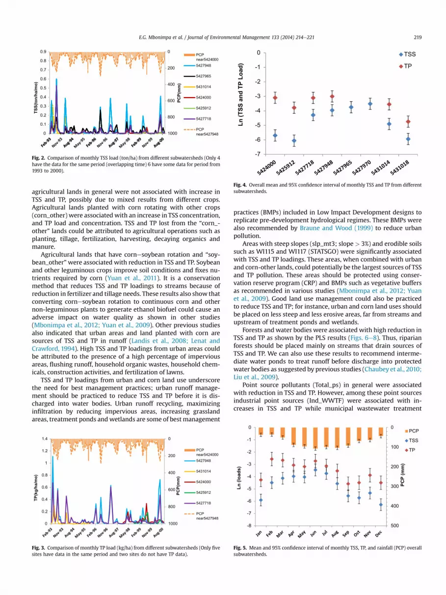
TP differences among subwatersheds enable determination ofsources of TSS and TP using landscape characteristics. Monthly TSSand TP measured at different USGS sites and NOAA-monitoredprecipitations at different parts of the watershed were comparedusing ANOVA also. The overall ANOVA-P value (<0.0001) from thecomparison of TSS among monitoring sites and for differentmonths was less than the reference alpha value (P ¼ 0.05), whichindicates monthly TSS and TP loads from the independent sub-watersheds (monitoring sites) and different months are signifi-cantly different. Multiple comparisons of means indicated thatsome subwatersheds have similarities in TSS and TP however; forexample, no significant difference in TSS among sites 5427970,5427965, 5427718 and 5427948 (Fig. 4) were found, and there wasno significant difference between sites 5431018, 5424000 and5425912. For TP however, 5431018 was the only subwatershed thatwas significantly different from the rest.

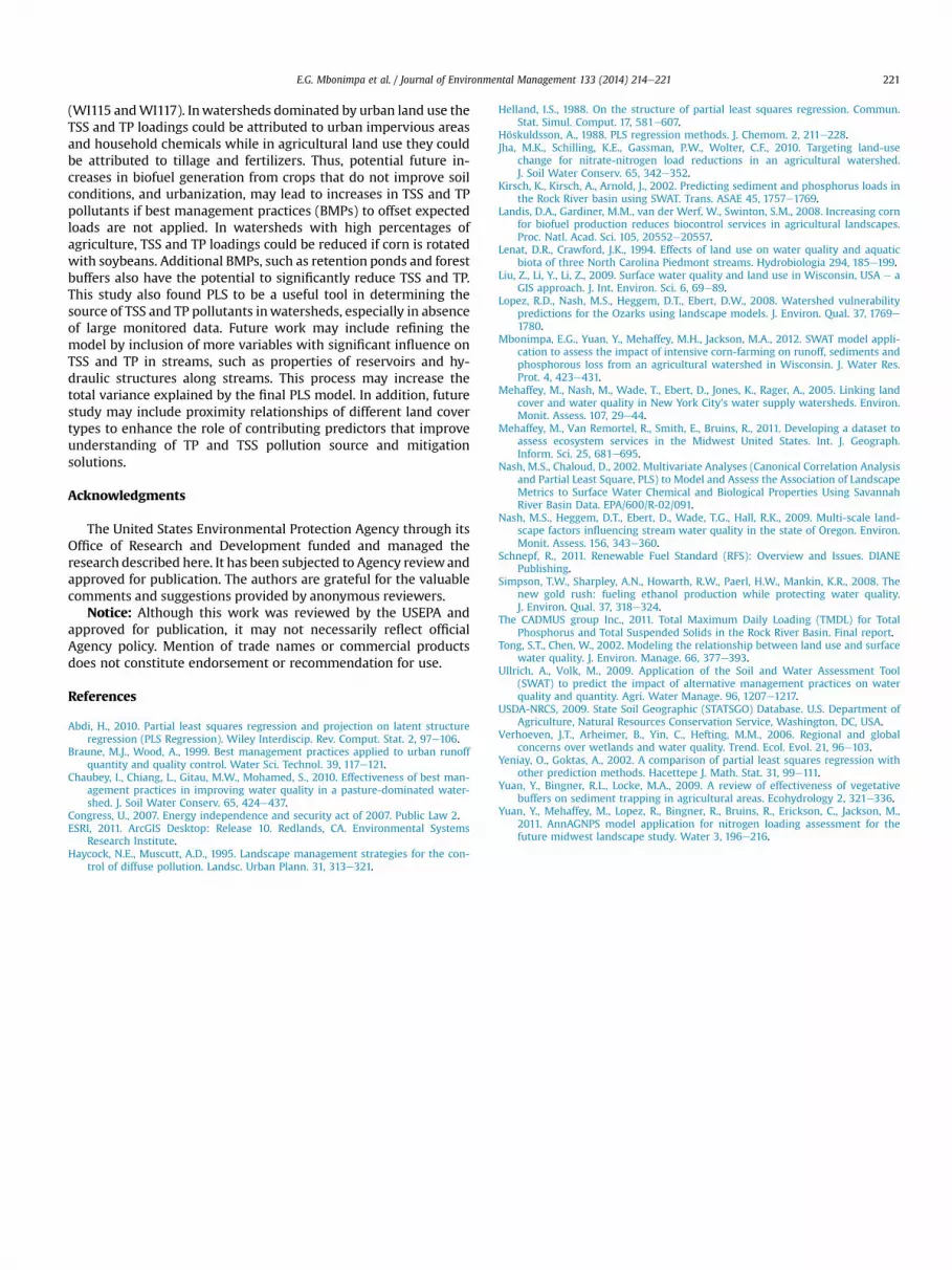
The comparison among months of the year for all sub-watersheds showed similarities betweenmonthly TSS loading fromFebruary through August (Fig. 5). This period’s TSS was significantlydifferent from the September through January period. Elevated TSSfrom February through August could be attributed to snow melt inFebruary and early March, agricultural activities in April or May(such as tillage or planting), and increase in precipitation(Mbonimpa et al., 2012). Frozen streams due to low temperatures inthe period of November through January also hinder TSS transport.For TP, when months that ANOVA found to have similarities inmonthly TP loading are grouped, the group of September, October,and December was significantly different from the group ofFebruary to July, but has similarities with January, August andNovember. August’s and November’s TP loads were not signifi-cantly different from other groups. Overall months with high TSSand TP also received high precipitation, except February’s and

Table 5Slope distribution (in percent of drainage area).

Site Slope (% of total area)

<3% �3%

5424000 48.73 51.275425912 69.83 30.175427718 61.52 38.485427948 37.70 62.305427965 34.40 65.605427970 36.29 63.715431018 77.11 22.895431014 94.30 5.70

March’s TP loads which were higher. This elevated amount of TPmay be due to snow melt. Runoff generated by snow melt couldpromote transport of sediment and phosphorus. In addition,anthropogenic activities such as agricultural fertilization in April orMay (Mbonimpa et al., 2012) may results in elevated TP loading.The similarities in trends between TSS and TP on Fig. 5, loweramounts in January and higher amounts in June, could be attributedto phosphorus and soil particle interaction. Phosphorus is added tothe soil either in mineral form through fertilization (as phosphateion) or organic form (manure and decaying plant residue), themineral (soluble) form is unstable and a large portion binds to ionicsoil particles. The rest is taken by plant roots or immobilized intoorganic form by bacteria. Though a small portion of organic phos-phorus is mineralized by bacteria, it is usually stable and insoluble,and transported together with sediment by water runoff.

ANOVA analysis of monthly precipitations found no significantdifferences between the watershed’s three weather stations.

3.4. PLS results

The PLS regression results, depicted in Figs. 6e8 described howTSS and TP are associated with various landscape predictors (Fig. 8shows water quality associations with only land use to check thePLS results for one type of landscape characteristic). Regressioncoefficients indicated that urban land use highly influences TSS andTP loadings. The results indicated that Rock River watershed

Urban UrbanWetlands WetlandsWater bodies WaterForests, Shrubs, Grass Forest_otherTerrain with slopes lower than 3% Slp_lt3Terrain with slopes higher than 3% Slp_mt3Concentrated animal feeding operations CAFOsIndustrial point source or industrial

wastewater treatment facility outletInd_WWTF

Municipal wastewater treatmentfacility outlet

Mun_WWTF

Total number of point sources Total_psSTATSGO soil types WI069, WI091, WI115, WI116,

WI117, WI118, WI120, WI122,WI124, WI125, WI126,WIW-water

0

0.1

0.2

0.3

0.4

0.5

0.6

0.7

0.8

0.9

TS

S(to

n/h

a/m

o)

0

200

400

600

800

1000

PC

P(m

m)

PCPnear54245427948

5427965

5431014

5424000

5425912

5427718

PCPnear54279

000

48

Fig. 2. Comparison of monthly TSS load (ton/ha) from different subwatersheds (Only 4have the data for the same period (overlapping time) 6 have some data for period from1993 to 2000).

-7

-6

-5

-4

-3

-2

-1

0

Ln

(T

SS

an

d T

P L

oa

d)

TSS

TP

Fig. 4. Overall mean and 95% confidence interval of monthly TSS and TP from differentsubwatersheds.

E.G. Mbonimpa et al. / Journal of Environmental Management 133 (2014) 214e221 219

agricultural lands in general were not associated with increase inTSS and TP, possibly due to mixed results from different crops.Agricultural lands planted with corn rotating with other crops(corn_other) were associatedwith an increase in TSS concentration,and TP load and concentration. TSS and TP lost from the “corn_-other” lands could be attributed to agricultural operations such asplanting, tillage, fertilization, harvesting, decaying organics andmanure.

Agricultural lands that have cornesoybean rotation and “soy-bean_other”were associated with reduction in TSS and TP. Soybeanand other leguminous crops improve soil conditions and fixes nu-trients required by corn (Yuan et al., 2011). It is a conservationmethod that reduces TSS and TP loadings to streams because ofreduction in fertilizer and tillage needs. These results also show thatconverting cornesoybean rotation to continuous corn and othernon-leguminous plants to generate ethanol biofuel could cause anadverse impact on water quality as shown in other studies(Mbonimpa et al., 2012; Yuan et al., 2009). Other previous studiesalso indicated that urban areas and land planted with corn aresources of TSS and TP in runoff (Landis et al., 2008; Lenat andCrawford, 1994). High TSS and TP loadings from urban areas couldbe attributed to the presence of a high percentage of imperviousareas, flushing runoff, household organic wastes, household chem-icals, construction activities, and fertilization of lawns.

TSS and TP loadings from urban and corn land use underscorethe need for best management practices; urban runoff manage-ment should be practiced to reduce TSS and TP before it is dis-charged into water bodies. Urban runoff recycling, maximizinginfiltration by reducing impervious areas, increasing grasslandareas, treatment ponds andwetlands are some of bestmanagement

0

200

400

600

800

10000

0.2

0.4

0.6

0.8

1

1.2

1.4

PC

P(m

m)

TP

(k

g/h

a/m

o)

PCPnear54240005427948

5431014

5424000

5425912

5427718

PCPnear5427948

Fig. 3. Comparison of monthly TP load (kg/ha) from different subwatersheds (Only fivesites have data in the same period and two sites do not have TP data).

practices (BMPs) included in Low Impact Development designs toreplicate pre-development hydrological regimes. These BMPs werealso recommended by Braune and Wood (1999) to reduce urbanpollution.

Areas with steep slopes (slp_mt3; slope > 3%) and erodible soilssuch as WI115 and WI117 (STATSGO) were significantly associatedwith TSS and TP loadings. These areas, when combined with urbanand corn-other lands, could potentially be the largest sources of TSSand TP pollution. These areas should be protected using conser-vation reserve program (CRP) and BMPs such as vegetative buffersas recommended in various studies (Mbonimpa et al., 2012; Yuanet al., 2009). Good land use management could also be practicedto reduce TSS and TP; for instance, urban and corn land uses shouldbe placed on less steep and less erosive areas, far from streams andupstream of treatment ponds and wetlands.

Forests and water bodies were associated with high reduction inTSS and TP as shown by the PLS results (Figs. 6e8). Thus, riparianforests should be placed mainly on streams that drain sources ofTSS and TP. We can also use these results to recommend interme-diate water ponds to treat runoff before discharge into protectedwater bodies as suggested by previous studies (Chaubey et al., 2010;Liu et al., 2009).

Point source pollutants (Total_ps) in general were associatedwith reduction in TSS and TP. However, among these point sourcesindustrial point sources (Ind_WWTF) were associated with in-creases in TSS and TP while municipal wastewater treatment

0

100

200

300

400

500-8

-7

-6

-5

-4

-3

-2

-1

0

PC

P (m

m)

Ln

(lo

ad

s)

PCP

TSS

TP

Fig. 5. Mean and 95% confidence interval of monthly TSS, TP, and rainfall (PCP) overallsubwatersheds.

-0.2000

-0.1500

-0.1000

-0.0500

0.0000

0.0500

0.1000

0.1500

0.2000

0.2500

Co

efficien

t

TSS load

TSS conc

Slope

Point

sources

Soil types

Land use

Fig. 6. PLS regression coefficients of each predictor on TSS load and TSS concentration(a missing column means the predictor has zero coefficient).

-0.8

-0.6

-0.4

-0.2

0

0.2

0.4

Co

effic

ie

nt

TSS conc

TP conc

Fig. 8. PLS regression coefficients of land cover predictors on TSS and TPconcentrations.

E.G. Mbonimpa et al. / Journal of Environmental Management 133 (2014) 214e221220

facility outlets (Mun_WWTF) and concentrated animal feedingoperations (CAFOs) were associated with reduction in TSS and TP.This could be due to the fact that municipal wastewater effluentshave negligible TSS and TP after treatment while industrialwastewater has higher pollutant contents in discharging waters.Many factors can affect the pollutant loading from wastewaterdischarges; such as storms, time of the year, and type of facility.Secondly, Wisconsin regulations require that regulated CAFOs(1000 animals or more) have no discharge of pollutants to streams,unless caused by a catastrophic storm; a storm with 24-h durationexceeding the 25-year recurrence frequency (CADMUS group Inc.,2011). Thus, CAFOs did not have positive association with TPalthough they are known to generate wastes containing TP.

Weak association between corn land use and TSS/TP (Figs. 6e8)from PLS results could be caused by factors on which we did nothave data; such as application of conservation measures and BMPs,and localized stream erosion or legacy phosphorus that make thereceiving streams have higher TP and TSS than runoff from agri-cultural fields. Mixed positive and negative associations of wet-lands with TSS and TP could be attributed to the fact that large partsof wetlands vary from dry grass lands during dry periods to watersubmerged during wet periods. For instance, cattle and deer haveaccess to dry parts and can contribute TP and TSS to streams;wetlands are also known to reduce upstream nutrients due to up-take by wetland flora. In addition, there could errors involved indata collection and uncertainty in data used for statistical analysis.Furthermore, the PLS model showed that around 10e20% of vari-ation in TP and TSS could not be explained by used predictors. Thiscould be due to other factors not included as predictors because ofdifficulties in some data collection. Those factors could involveparameters related towater bodies, because main drainage streamsin this study watershed pass through a chain of lakes, marshes andreservoirs, some with flow control structures such as dams. The

-0.2000

-0.1500

-0.1000

-0.0500

0.0000

0.0500

0.1000

0.1500

0.2000

0.2500

Co

efficien

t

TP load

TP conc

Land use Soil types Slope

Point

Sources

Fig. 7. PLS regression coefficients of each predictor on TP load and TP concentration.

location of these water bodies with respect to other land uses alsowould affect the response at the outlet. The use of static land useand land cover maps might have also introduced errors becauseland use varies over time. It was also observed that two sites5427965 and 5427970 with roughly homogeneous land use; theirdrainage areas are almost entirely constituted by urban land use(83 and 96%, respectively), reduced accuracy of prediction by thePLS model. Uncertainty in response and predictor data also affectsregression results. For instance, response data could introduce er-rors because some response data from various monitoring siteswere not collected during the same time periods.

Differences in PLS analysis results were also noticed betweenTSS/TP concentration and loading. Concentration does not take intoaccount streams flow rate even though it could be affected by it.Analysis with of TSS/TP concentration could be affected if sub-watersheds receive precipitation with large differences in intensityand distribution. However, ANOVA indicated that precipitation didnot differ significantly among the three weather stations in thewatershed. PLS analysis with TSS/TP expressed in loading could beaffected if subwatersheds have differences in the presence andlocation of hydraulic structures such as dams, reservoirs and otherwater flow obstructing systems. These structures hold water insidethe watershed and could cause a lag in TSS and TP response at theoutlets. Thus, TSS or TP readings for a certain month for somesubwatersheds could be comparable to previous months’ readingsin other subwatersheds. These hydraulic systems could also accel-erate deposition of sediment or dissolution or decomposition ofphosphorus.

Also, the geographical position of different landscape features inthe watershed could affect results. For instance, a wetland up-stream of agriculture would not show improvement of watercompared to wetlands located downstream of agricultural areas.Thus, if the position of landscape features is not included inregression as variables it could affect regression results. In addition,Rock River watersheds comprise many internal drained areas thatsometimes do not contribute water to the watershed outlet (Kirschet al., 2002). The position, number and the size of these areas andthe hydraulic systems mentioned earlier should be included inregression as variables, but the information was difficult to collectto be included into the analyses.

4. Conclusions

The conclusions from this study are that urban land use and cornrotating with other crops, except legumes such as soybeans, wereassociated with TSS and TP loadings increases in the Rock Riverwatershed. These loadings are also influenced by steep terrain(slopes higher than three percent) and soils with higher erodibility

E.G. Mbonimpa et al. / Journal of Environmental Management 133 (2014) 214e221 221

(WI115 andWI117). Inwatersheds dominated by urban land use theTSS and TP loadings could be attributed to urban impervious areasand household chemicals while in agricultural land use they couldbe attributed to tillage and fertilizers. Thus, potential future in-creases in biofuel generation from crops that do not improve soilconditions, and urbanization, may lead to increases in TSS and TPpollutants if best management practices (BMPs) to offset expectedloads are not applied. In watersheds with high percentages ofagriculture, TSS and TP loadings could be reduced if corn is rotatedwith soybeans. Additional BMPs, such as retention ponds and forestbuffers also have the potential to significantly reduce TSS and TP.This study also found PLS to be a useful tool in determining thesource of TSS and TP pollutants inwatersheds, especially in absenceof large monitored data. Future work may include refining themodel by inclusion of more variables with significant influence onTSS and TP in streams, such as properties of reservoirs and hy-draulic structures along streams. This process may increase thetotal variance explained by the final PLS model. In addition, futurestudy may include proximity relationships of different land covertypes to enhance the role of contributing predictors that improveunderstanding of TP and TSS pollution source and mitigationsolutions.

Acknowledgments

The United States Environmental Protection Agency through itsOffice of Research and Development funded and managed theresearch described here. It has been subjected to Agency reviewandapproved for publication. The authors are grateful for the valuablecomments and suggestions provided by anonymous reviewers.

Notice: Although this work was reviewed by the USEPA andapproved for publication, it may not necessarily reflect officialAgency policy. Mention of trade names or commercial productsdoes not constitute endorsement or recommendation for use.

References

Abdi, H., 2010. Partial least squares regression and projection on latent structureregression (PLS Regression). Wiley Interdiscip. Rev. Comput. Stat. 2, 97e106.

Braune, M.J., Wood, A., 1999. Best management practices applied to urban runoffquantity and quality control. Water Sci. Technol. 39, 117e121.

Chaubey, I., Chiang, L., Gitau, M.W., Mohamed, S., 2010. Effectiveness of best man-agement practices in improving water quality in a pasture-dominated water-shed. J. Soil Water Conserv. 65, 424e437.

Congress, U., 2007. Energy independence and security act of 2007. Public Law 2.ESRI, 2011. ArcGIS Desktop: Release 10. Redlands, CA. Environmental Systems

Research Institute.Haycock, N.E., Muscutt, A.D., 1995. Landscape management strategies for the con-

trol of diffuse pollution. Landsc. Urban Plann. 31, 313e321.

Helland, I.S., 1988. On the structure of partial least squares regression. Commun.Stat. Simul. Comput. 17, 581e607.

Höskuldsson, A., 1988. PLS regression methods. J. Chemom. 2, 211e228.Jha, M.K., Schilling, K.E., Gassman, P.W., Wolter, C.F., 2010. Targeting land-use

change for nitrate-nitrogen load reductions in an agricultural watershed.J. Soil Water Conserv. 65, 342e352.

Kirsch, K., Kirsch, A., Arnold, J., 2002. Predicting sediment and phosphorus loads inthe Rock River basin using SWAT. Trans. ASAE 45, 1757e1769.

Landis, D.A., Gardiner, M.M., van der Werf, W., Swinton, S.M., 2008. Increasing cornfor biofuel production reduces biocontrol services in agricultural landscapes.Proc. Natl. Acad. Sci. 105, 20552e20557.

Lenat, D.R., Crawford, J.K., 1994. Effects of land use on water quality and aquaticbiota of three North Carolina Piedmont streams. Hydrobiologia 294, 185e199.

Liu, Z., Li, Y., Li, Z., 2009. Surface water quality and land use in Wisconsin, USA e aGIS approach. J. Int. Environ. Sci. 6, 69e89.

Lopez, R.D., Nash, M.S., Heggem, D.T., Ebert, D.W., 2008. Watershed vulnerabilitypredictions for the Ozarks using landscape models. J. Environ. Qual. 37, 1769e1780.

Mbonimpa, E.G., Yuan, Y., Mehaffey, M.H., Jackson, M.A., 2012. SWAT model appli-cation to assess the impact of intensive corn-farming on runoff, sediments andphosphorous loss from an agricultural watershed in Wisconsin. J. Water Res.Prot. 4, 423e431.

Mehaffey, M., Nash, M., Wade, T., Ebert, D., Jones, K., Rager, A., 2005. Linking landcover and water quality in New York City’s water supply watersheds. Environ.Monit. Assess. 107, 29e44.

Mehaffey, M., Van Remortel, R., Smith, E., Bruins, R., 2011. Developing a dataset toassess ecosystem services in the Midwest United States. Int. J. Geograph.Inform. Sci. 25, 681e695.

Nash, M.S., Chaloud, D., 2002. Multivariate Analyses (Canonical Correlation Analysisand Partial Least Square, PLS) to Model and Assess the Association of LandscapeMetrics to Surface Water Chemical and Biological Properties Using SavannahRiver Basin Data. EPA/600/R-02/091.

Nash, M.S., Heggem, D.T., Ebert, D., Wade, T.G., Hall, R.K., 2009. Multi-scale land-scape factors influencing stream water quality in the state of Oregon. Environ.Monit. Assess. 156, 343e360.

Schnepf, R., 2011. Renewable Fuel Standard (RFS): Overview and Issues. DIANEPublishing.

Simpson, T.W., Sharpley, A.N., Howarth, R.W., Paerl, H.W., Mankin, K.R., 2008. Thenew gold rush: fueling ethanol production while protecting water quality.J. Environ. Qual. 37, 318e324.

The CADMUS group Inc., 2011. Total Maximum Daily Loading (TMDL) for TotalPhosphorus and Total Suspended Solids in the Rock River Basin. Final report.

Tong, S.T., Chen, W., 2002. Modeling the relationship between land use and surfacewater quality. J. Environ. Manage. 66, 377e393.

Ullrich, A., Volk, M., 2009. Application of the Soil and Water Assessment Tool(SWAT) to predict the impact of alternative management practices on waterquality and quantity. Agri. Water Manage. 96, 1207e1217.

USDA-NRCS, 2009. State Soil Geographic (STATSGO) Database. U.S. Department ofAgriculture, Natural Resources Conservation Service, Washington, DC, USA.

Verhoeven, J.T., Arheimer, B., Yin, C., Hefting, M.M., 2006. Regional and globalconcerns over wetlands and water quality. Trend. Ecol. Evol. 21, 96e103.

Yeniay, O., Goktas, A., 2002. A comparison of partial least squares regression withother prediction methods. Hacettepe J. Math. Stat. 31, 99e111.

Yuan, Y., Bingner, R.L., Locke, M.A., 2009. A review of effectiveness of vegetativebuffers on sediment trapping in agricultural areas. Ecohydrology 2, 321e336.

Yuan, Y., Mehaffey, M., Lopez, R., Bingner, R., Bruins, R., Erickson, C., Jackson, M.,2011. AnnAGNPS model application for nitrogen loading assessment for thefuture midwest landscape study. Water 3, 196e216.