SELLING PICASSO PAINTINGS:

THE EFFICIENCY OF AUCTION HOUSES1

Finn R. Førsund

Department of Economics, University of Oslo, Norway

and

Visiting Fellow ICER, Turin, Italy

Email: f.r.forsund@econ.uio.no

and

Roberto Zanola

Department of Public Policy and Public Choice,

University of Eastern Piedmont, Italy.

Email: zanola@cicladi.unipmn.it

May 17, 2001

Abstract. Previous works applying hedonic price technique to determine theformation of auction prices of objects of art have found no conclusive result about theimpact of auction houses on final prices. In these studies the object of art has been theunit, and influence of auction houses is analysed by testing whether auction houseimpact on price is significant or not within a framework of central tendencies. In orderto focus on auction houses as a unit we have applied a benchmarking technique, DEA,developed for efficiency studies. Categorial and continuous variables are used asinputs and auction prices as outputs. Performance indicators are defined andcalculated giving an insight into auction house differences impossible to obtain usinghedonic price approach.

Key words: painting, auction house, hedonic price, DEA, efficiency.

JEL classification: C6, D2, Z1. 1 A first version of the paper was written while the first author was a visiting fellow at InternationalCentre for Economic Research (ICER), Turin, January – March 2001. It is part of the project“Cheaper and better?” at the Frisch Centre, financed by the Norwegian Research Council, and of theproject on “Cultural goods” financed by the Italian Research Council. We are indebted to Dag FjeldEdvardsen for help with using the DEA software package of the Frisch Centre.

2

1. Introduction

In November 1989 Picasso’s “Au lapin agile” was sold at Sotheby’s New York for $37

million. In November 1989 Picasso’s “Les Noces de Pierrette” was sold at Drouot Paris

for $46,9 million. In November 1995 Picasso’s “Le miroir” was sold at Christie's New

York for $18,2 million. From such sensational prices, which are sometimes highlighted

in the media, an intriguing question arises about whether there is a relationship between

the price and the auction house where the painting is sold.

There is some evidence on influence of auction houses in the literature. Pesando (1993),

using information on repeat sales of identical prints, shows that there is a tendency for

prices paid by buyers to be systematically higher at certain auction houses. In particular,

prints sold at Sotheby’s in New York perform average prices 14 per cent higher than the

prices of identical prints sold at Christie’s in New York. However, to the extent that

paintings are different from each other, a similar arbitrage study cannot be performed

with reference to the market for paintings (Renneboog and Van Houtte, 2000).

The only approach that has been developed so far to address this issue is the hedonic

price technique.2 The hedonic price technique has been used extensively to investigate

the investment value of visual art collectibles, such as paintings (Anderson, 1974; Frey

and Pommerehene, 1989; Buelens and Ginsburgh, 1993; Chanel et al., 1996; Agnello

and Pierce, 1999; Renneboog and Van Houtte, 2000), prints (Pesando, 1993), and

sculptures (Locatelli-Biey and Zanola, 2001).

In the hedonic price model the influence on the auction price of single art objects of

various variables is found by regressing the auction price on this set of variables

regarded as determinants of price. The variables are both categorical variables, like

reputation of artist, condition of object, style, provenance and exhibitions, authenticity

(signed or not), medium, and continuous variables, like size measured in various ways.

The auction house handling the art object is one of the categorical variables that have

3

been used when trying to determine their influence (Czujack, 1997). The partial impact

of price of each variable including characteristics or attributes are then associated with

parameters of the estimated regression function. The “implicit price” or value of each

characteristic is based on the derivative of the hedonic price function with respect to the

work’s attribute (Combris et al., 1997). Chanel et al. (1996) perform the hedonic

regression method using all sales (not including re-sales) of Impressionists, Post-

impressionists and their “followers” sold at auctions between 1855 and 1970. The

coefficients associated with auction house dummies show that Christie’s New York

perform rather poorly, some 10 to 20 per cent less than at Sotheby’s. Agnello and Pierce

(1998) use data on over 25,000 U.S. paintings sold at auction from 1971 to 1996.

Sotheby’s New York and Christie’s New York increase price by 68 per cent and 54 per

cent, respectively, over all other auction houses. By contrast, Renneboog and Van

Houtte (2000), by using a large database of Belgian school’s works sold during the

period 1970-1997, find that the highest prices are achieved at Christie’s New York,

followed by Sotheby’s New York. Concerning London subsidiaries of the same auction

houses prices are lower than their American counterparts, but higher than in Continental

Europe.

Differently from previous works, Czujack (1997) only examines the market for

Picasso’s paintings sold at auction between 1963 and 1994. She finds no significant

differences between auction houses. In fact, even if Sotheby’s New York is more

successful in attracting vendors, the higher price level of Sotheby’s New York is only

due to dimension, medium, year of painting, and so on.

However, the hedonic technique only represents an indirect approach to analyse the

eventual existence of a relationship between price and auction houses since it does not

focus on the latter as units of observation, but on the individual painting. An alternative

way of addressing the performance of auction houses is to focus on the auction house as

a “producer”: art objects of various characteristics are received as inputs and the auction

prices obtained are then the outputs3. For a given set of art objects an auction house is

more efficient the higher the auction price is. In order to compare an auction house with 2 See Griliches (1961, 1990) and Rosen (1974), among others, for a general introduction.

4

the best performing ones and to estimate how much better results an auction house

could have if it is as good as the best, a benchmark in the form of a best practice

production function can be established4. One could argue that it is the general demand

for the type of art object under investigation that determine the price and not the auction

house. But data shows that even for the same year prices for similar art objects differ

between auction houses, and concerning development over time one could claim that an

auction house should advice a client as to when the client should sell or buy. The

auction houses compete for customers. Art objects are not perishable goods! Predicting

booms and through years may be considered as a part of being efficient5.

An increasingly popular tool to investigate efficiency is Data Envelopment Analysis

(DEA)6, which allows us to handle both multiple inputs and multiple outputs, as is the

case for auction houses. The DEA uses linear programming techniques to construct a

non-parametric piecewise linear frontier, which envelops all the observations as tight as

possible subject to some basic assumptions on the production technology.

The purpose of this paper is to analyse the performances of auction houses by studying

the efficiency in “transforming” art objects with physical characteristics and attributes

into auction prices. The empirical analysis is based on information on selling price and

various input indicators of Picasso paintings as drawn from auctions held during the

period of sale 1988-1995 as registered in the 1995 edition of the Mayer International

Auction Records on CD-ROM.

The paper is organised as follows: In Section 2 we analyse the output oriented DEA

model used in this paper. Data and choice of variables are described in Section 3. The

results from applying the described methodology are shown in Section 4. Some

concluding remarks are provided in Section 5.

3 The internal inputs such as labour, offices, etc., are disregarded. If such information is availableanother approach is to define the net income of an auction house as the output and art objects andinternal resource as inputs.4 An alternative could be to focus on the difference between pre-auction estimates and realised pricesas a source of inefficiency. However, pre-auction estimates are not readily available to us.5 However, a client may force an auction house to sell against its advice.6 See e.g. Seiford (1996) for a bibliography of DEA applications.

5

2. The DEA model

2.1 A brief historical note

Efficiency is a core concept of microeconomics. In the seminal paper of Farrell (1957)

theory and tools for empirical efficiency analyses were introduced that are still at the

forefront of research on efficiency at the micro level of a production unit today. The two

key issues addressed were how to define efficiency and productivity, and how to

calculate the benchmark technology, and the efficiency and productivity measures. The

fundamental assumption was the possibility of inefficient operations, pointing to a

frontier production function concept as the benchmark, as opposed to a notion of

average performance underlying most of the econometric literature on the production

function up to the sale of the seminal contribution.

Farrell approached the two fundamental issues above in the following way:

i) efficiency measures were based on radial uniform contractions or expansions

from inefficient observations to the frontier;

ii) the production frontier was specified as the most pessimistic piecewise linear

envelopment of the data;

iii) the frontier was calculated through solving systems of linear equations (but not

using linear programming (LP) solution algorithms).

Both in Farrell (1957) and in the published discussion of his presentation some key

elements for statistical analyses were also pointed out. However, progress on this

frontier was not made until the contributions of Aigner and Chu (1968), Afriat (1972),

and Aigner, Lovell and Schmidt (1977), who introduced the composed error model

(independently introduced also in Meeusen and van den Broeck, 1977), to mention

some of the most influential contributions within estimation of parametric frontier

production functions.

6

Progress on the Farrell programming approach for the case of piecewise linear frontier

functions was not made until Charnes, Cooper and Rhodes (1978), where the expression

DEA for the LP approach was coined.7 The linear programming model formulated was

a generic one covering multiple outputs and inputs, and was quite superior to Farrell’s

applied unit isoquant approach in the case of a single output (Farrell's programme for

multiple outputs has never been implemented). The model was readily computable,

either using standard LP codes on mainframes or developing more efficient tailor-made

software. From the late 80s the number of applied analyses based on the DEA model

exploded (see Seiford, 1996). Main reasons for its popularity are ease of use and the

handling of multiple outputs, and the fact that no functional form for the frontier has to

be assumed.

The outputs from a DEA analysis are Farrell efficiency scores for each unit of

production, and identification of the peers of inefficient units; i.e. the efficient units that

serve as reference units when calculating the efficiency measure. When looking for

ways of improving performance these are the units to be studied.

2.2 Output oriented DEA model, CRS

The point of departure for the calculation of efficiency measures is the piecewise linear

frontier technology expressed by the following production possibility set:

(1)

where x is the input vector and y is the output vector, and in the last expression we have

introduced j points and index m for type of output and index n for type of input. The

variables λ j are non-negative weights or intensity variables defining frontier points.

Constant returns to scale (CRS) is assumed. Basic properties are that the production set

7 Note that some earlier contributions from agricultural economists at Berkley went unnoticed; see e.g.Boles (1967), (1971). See Førsund and Sarafoglou (2000) for the history of the evolution of the LPmodel.

{ }

{ }j0,nxx,myy:)y,x(

xbyproducedbecany:)y,x(S

j

J

1jnjjn

J

1jmmjj ∀≥λ∀λ≥∀≥λ

==

��==

7

is convex, includes all points and envelopment is done with minimum extrapolation, i.e.

the fit is as “tight” as possible.

The output oriented Farrell radial efficiency measure, E2i , for each unit, i of a set of j

observations, is calculated by solving the following linear program set up according to

the definition of the measure, with the necessary change that we solve for the inverse

measure φi = 1/ E2i in order to maintain a linear programming problem:

(2)

Each type of output is scaled up with the same factor, φi, until the frontier is reached

according to the (inverse) definition of the Farrell efficiency measure.

It should be noted that a general assumption underlying the rationale for comparing

different production units is that the inputs and outputs are indeed comparable, i.e. that

they are homogeneous. If xni is labour input measured in hours then these hours must be

comparable across the units. It would not be so meaningful an analysis if one unit has

highly educated employees while another has unskilled ones if we believe that marginal

productivity of these two types of labour are significantly different.

2.3 The treatment of categorical variables

It may be the case that variables are categorical, i.e. there are inputs and/or outputs of

certain types, e.g. type of education of labour, type of court cases being completed, etc.,

which are distinct and cannot be represented by continuous variables. In regression

models with one dependent variable and a set of explanatory variables, including

categorical ones, the categorical information is handled by using dummy variables (i.e.

0 if the unit is not of the type in question, 1 otherwise), and the partial impact on the

JiJj

Nnxx

Mmyy

ts

MaxE

j

J

jnjijni

J

jmiimjij

ii

,..,1,,..,1,0

,..,1,0

,..,1,0

..

1

1

1

2

==≥

=≥−

=≥−

=

�

�

=

=

λ

λ

φλ

φ

8

dependent variable of each characteristic may be identified (relative to a reference type

or group). The analogy with our production formulation is that the dependent variable is

a single output, and that the explanatory variables are the inputs.

In the DEA model a general way of handling such attributes may be to interpret them

as different types of inputs and/or outputs. Let zkj be a categorical characteristic k

(k=1,..,K) of unit j (j=1,..,J) regarding types of inputs, and let xnj be continuos input

variables of type n (n=1,..,N). We then have K×N different types of inputs; each

continuous variable is assigned to each of the K types of inputs. Each production unit

may employ fewer characteristics than the total number available, resulting in a value of

zero for the non-observed types of inputs. An extreme case would be that each unit j

employs only one type of labour as it is the case for education. Treatment of categorical

output characteristics will be the same.

A hierarchical structure has so far been imposed in the literature, leaving us with a

mixed integer LP programme if mix of differently ranked peers is not allowed (see the

seminal paper by Banker and Morey (1986), and also Kamakura, 1988). A standard LP

format of the DEA model can be used if a special aggregation of types into two groups

is done; according to lower or higher ordered types compared with the situation for the

unit under investigation. The procedure in Charnes et al. (1994) implies that all

differences between types of variables can be reduced to two, and the DEA model is

only run for the one subset relevant for the analysis. But then there are no restrictions on

the mixing of peers with lower ranked inputs, or higher ranked outputs respectively. It is

implicitly assumed that it makes sense to mix qualities in both these subsets. Without a

hierarchical ordering the formation of two subsets is not defendable, and with an

ordering one may, as in Kamakura (1988), question the procedure because mixes cannot

be observed.

Our approach is designed for situations when it is not natural to order categorical

variables hierarchically. A standard LP format of the DEA model can be used, if both

categorical and continuous variables are present, by writing out all the combinations of

the categorical variables as different types of inputs and/or outputs as demonstrated

above. Most units will then not have full sets of positive variables. Using a standard LP

DEA model of type (2) will then not in general give the same results (with respect to

9

efficiency scores and peers) as using the mixed integer-LP model of Banker and Morey

(1986) or the reformulation in Kamakura (1988), or the special aggregation introduced

in Charnes et al. (1994).

We will use a more general setting with no ordering of categories and investigate the

nature of the selected peers both in the input- and output dimension. The special cases

dealt with in the literature can easily be incorporated. If each unit has only one of the

possible types of inputs or outputs, and a comparison only with same or higher ranked

types is wanted, formation of new subsets of units as required in Charnes et al. (1994),

is not necessary, because employing the standard model with the full set of types of

variables will yield separate group results for units with same type of variable by

definition.

The following formal rules can be established in general for our case when calculating

either an input- or output oriented Farrell efficiency score for a unit (see Førsund,

2001):

i) the unit under investigation will only be compared with peer units having the

same or less types of inputs;

ii) a peer will have at least one type of input in common with the unit under

investigation;

iii) the unit under investigation may be compared with peer units having both more

or less types of outputs, but in the latter case the peer unit must have at least one

common type of output;

iv) in the set of peers all types of outputs of the unit under investigation must be

represented.

The general result for the characterisation of peers is that there is a basic asymmetry

between inputs and outputs, due to the inequality constraints going in opposite

directions and all variables restricted to being non-negative. Intuitively, more of inputs

reduce efficiency while more of outputs improve efficiency.

10

3. Data and choice of model

3.1 Data

The unit of analysis is the local branches of auction houses. However, there are only

four significant auction house units dealing in Picasso paintings, while all other houses

have been aggregated together. Hence, we are left with only five units of analysis:

Christie’s London, Christie’s New York, Sotheby’s London, Sotheby’s New York, and

Other auction houses.8

The data are compiled from auctions held during the sale period 1988-1995 as reported

in the 1995 edition of the Mayer International Auction Records on CD-ROM. Prices are

gross of the buyers’ and sellers’ transaction fees paid to auction houses. No information

is provided on the origin of the paintings and exhibitions of them. All paintings are

priced in U.S. dollars deflated by using the U.S. consumer price index (end of 1990 =

100) to remove the general trend of inflation. For the sake of simplicity, we assume that

all sales occur at the end of each period.

3.2 Choice of model

The purpose of this study is to analyse the performances of auction houses by studying

the efficiency in “transforming” an art object with physical characteristics and attributes

into auction prices. Since we have a cross-section and sale series data set, an analysis of

efficiency change within each period and a productivity analysis over sale by using a

Malmquist productivity index approach can be performed (see e.g. Färe et al., 1998).

However, since we are left with only five units of analysis, in order to achieve results of

interest we assume that the same frontier technology is valid for all periods. This can be

11

defended because technological change is not so relevant for the special type of

production process we are dealing with. If it had turned out to be a systematic sale trend

in sales prices over this period this trend could have been removed from the data, but

this has not been the case. We are therefore assuming an inter-temporal frontier

according to the terminology of Tulkens and van den Eeckaut (1995). Due to the

assumption of inter-temporal frontier the calculation of Malmquist productivity indices

will be identical to setting up the problem as a DEA programme as shown in Section 2.9

As the unit of analysis we have an auction house observed for a specific sales period.

We have sixteen sales periods and five auction houses, so this gives us eighty units of

analysis as a maximum if in each sale period all houses have sales. There are periods

when some auction houses do not have sales leaving us with 63 units in the analysis.

This number of units gives us some scope for introducing variables of interest. Czujack

(1997) suggests the working period and the dimension variables as indicators of

painting quality and hence as factors affecting the final price of Picasso paintings.10 The

rationale for including the listed variables may be noted briefly. Picasso’s production is

characterised by different working periods, which vary strongly with respect to quality,

numbers of items and influence on the art. Three different working period are identified:

period 1, which commands the highest prices and encompasses Childhood and Youth

(1881-1901), Blue and Rose Period (1902-1906), and Analytical and Synthetic Cubism

(1907-1915); period 2, composed by Camera and Classicism (1916-1924), Juggler of

the Form (1925-1936), and Guernica and the “Style Picasso” (1937-1943); and period 3,

whose prices are the lowest and encompasses Politics and Art (1944-1953) and The Old

Picasso (1954-1973).

As far as size variables are regarded, the total square centimetre of paintings, and the

inverse of the average value of surface squared, will be used. The higher the surface the

higher the auction price is. However, hedonic price models show that there is a

decreasing returns to size for a painting, which is captured in the DEA model by using

the inverse form of the surface, squared. A contributing factor is that smaller sized 8 Drout France, Phillips London, Finarte Italy, among others.9 In general a Malmquist index can be decomposed multiplicatively into frontier shift and catching-up,but since technological changes is by assumption ruled out we are left with efficiency changes only.

12

paintings can more easily be hanged on walls of private homes. Due to the non-linear

effect on prices captured in this way a constant returns to scale model is assumed.

The aggregated auction prices within each group of paintings are used as outputs.

Restricting ourselves to three periods and the two media given on the CD-ROM, oil on

canvas and oil on other material, will yield 3x2 = 6 different types of paintings. These

represent the categorical variables. For each type we have the surface and surface

squared yielding twelve continuous input variables. The same types of inputs are also

used as types of outputs, leaving us with six output variables and 18 variables in total.

However, due to dimensionality problems we have been forced to reduce the number of

variables, and we have chosen to deleted the group of oil on other material, leaving us

with six input variables and three output variables; nine variables in total.

Table 1 lists the variables and the summary statistics. We see that on average the first

period paintings are the smallest, and size increasing considerably with factors of 2.2

and 3.5 respectively during the second and third period. The largest sales in area also

follow this pattern. The mean sales values have the inverse relationship, Period 1

pictures being priced higher with factors of 2.75 and 5.75 respectively for the other two

periods. The maximum sales value (a single painting) is $ 48 million from the first

period, followed by $ 43 million from the second and $ 16 million from the third.

Table 1. The data. Unit: auction house per auction period(inverse of squared area scaled with 104,sales value in 100,000 1990 dollars)

PicassoPeriod

Variable Mean St. dev. Max Min

InputsArea in dm2 46.87 178.75 227.05 3.86Period 1

1881-1915 Average inverse(area)2

78.62 170.05 672.69 0.19

Area in dm2 103.34 106.20 593.04 2.52Period 21916-1943 Average inverse

(area)2112.82 326.13 1574.70 0.06

Area in dm2 163.10 173.64 929.40 7.95Period 31944-1973 Average inverse

(area)26.37 21.71 158.10 0.08

10 Additional factors, which are suggested to affect cost, such as signature, Zervos catalogue raisonnénumber, exhibition, resales, and provenance, have not been considered in this study due to data anddimensionality problems. Hence, a word of caution for the interpretation of the DEA results.

13

OutputsPeriod 1 Sales value 126.96 184.40 484.69 4.02Period 2 Sales value 46.04 73.70 429.63 0.38Period 3 Sales value 22.07 30.92 162.79 0.64

4. Results

In this section the efficiency scores for each unit of analysis are reported. We will then

proceed to utilise these results to shed some light on the issues discussed in Section 2.

The DEA model comprising six input and three output variables is computed using the

FrischDEA software package11.

4.1 The auction house efficiency scores

The distribution of efficiency scores, sorted from the most inefficient unit to fully

efficient ones, is presented in Figure 1. Each bar represents a unit. The size of each

11 This package is developed at the Frisch Centre, Oslo.

0.0

0.1

0.2

0.3

0.4

0.5

0.6

0.7

0.8

0.9

1.0

0 1000 2000 3000 4000 5000Total sales in $100,000

Effic

ienc

y sc

ore

14

Figure 1. The efficiency distribution

Unit, measured in sales, is proportional to the width of each bar. The efficiency score is

measured on the vertical axis and the sales value accumulated on the horizontal axis.

We note that about one quarter of the total sales value of $522 million (1990

Dollars) refer to inefficient units. The inefficiency distribution stretches from 0.13 to 1.

The first part from 0.13 to 0.5 consists of small units. The next group of larger, but

below medium sized units, is distributed in the interval 0.6 to 0.7 of the efficiency score.

The third group of mainly medium sized units and some smaller units stretches from 0.7

to 1. It is notable that the efficient group, although dominated by medium- and the

largest sized units, also comprises some small units.

Of the 63 units 23 are fully efficient and one unit has a score of 0.9996 (this is the first

unit from the left in Figure 1 to visually be at the efficiency score level of one, the fully

efficient units are sorted, somewhat arbitrarily, according to place in the data-file). Of

the 23 efficient units five are self-evaluators. A unit may be self-evaluator either

because it has one or more especially large (or large or small in absolute values in the

case of VRS) dimensions as to output- and/or input mix, placing it on the edge of the

facets comprising the frontier, or it may be interior due to lack of inefficient referent

units. The nature of the self-evaluators turns out to be extreme self-evaluators for all

(see Edvardsen et al. (2001) for the method of determination).

4.2 The inter-temporal pattern of efficiency

The pattern of efficiency score over time or each auction house is reported in Table 2.

The 58 formal units are grouped under each auction house. Sotheby's London are

represented only in nine of the 16 sales periods, while Sotheby's New York have sales

in all sale periods, as well as Christie's New York, except one period without sales.

Christie's London has sales in 11 periods and Others in 12.

Looking at the general pattern over periods of efficient units we can identify good and

bad years. In the first period (1988:I) scores are rather low and the two efficient ones are

extreme self-evaluators. In the next period efficiency starts to pick up with two efficient

15

units of the four with sales. In the sales period 3(1989:I) two of the five auction houses

are efficient, but both efficient ones are self-evaluators, while for period 4 (1989:II) two

of the auction houses are efficient (but two are self-evaluators). In the next sales period

5 (1990:I) four of the five auction houses are efficient, and in period 6 (1990:II) two out

of the four auction houses are efficient. These last four sales periods have been

Table 2. The inter temporal pattern of efficiency

Auction house efficiency scores

YEAR Sales

period

Christie’s

New York

(1)

Christie’s

London

(2)

Sotheby’s

New York

(3)

Sotheby’s

London

(4)

Others

(5)

1988:I 1 0.39 1* 0.61 0.65 1*

1988:II 2 1 0.50 1 0.93 -

1989:I 3 0.60 1.00 1 1 1

1989:II 4 1 1* 1 1 1*

1990:I 5 1 1 0.71 1 0.81

1990:II 6 1 - 0.97 0.41 1

1991:I 7 - - 0.46 1 0.26

1991:II 8 0.31 0.79 0.34 - 0.77

1992:I 9 0.79 - 0.14 - -

1992:II 10 0.29 0.32 0.66 - 0.30

1993:I 11 1 0.91 1 - -

1993:II 12 0.32 0.43 0.66 - -

1994:I 13 0.65 0.25 0.70 0.26 0.32

1994:II 14 0.22 0.38 1* - 0.21

1995:I 15 1 - 1 - 0.20

1995:II 16 0.89 - 0.93 0.19 0.13∗ Self-evaluator

identified as the maximum expansion of the boom years in general.12 For the rest of the

sales periods only one, or two at most, auction houses are efficient. Years without

efficient units are 1991:II, 1992:I, 1992:II, 1993:II, 1994:I and 1995:II. A falling market

set in 1991 and it remained weak for some years in general. The sale periods 1991:II,

1992:I, 1992:II and 1993:II seem especially weak in view of the low efficiency scores.

16

But it is remarkable that we have efficient units in 1991:I (Sotheby's London), and in

1993:I (Christie's New York and Sotheby's New York. In general, the market picks up

in 1994-1995. Our units show efficiency in 1995:I with two of three being efficient,

while the one efficient in 1994:II is a self-evaluator, and the other scores are especially

low. The recovery in the Picasso market seems to be one year later than in general. A

distinct feature of the later periods is the uneven levels of efficiency scores. It seems

that better sales have been especially picked up by both the New York auction houses,

Christie's New York and Sotheby's New York having both 1995:I as efficient sale

periods and maintaining high levels of efficiency in 1995:II. Sotheby's London (no sale

in 1995:I) and Other auction houses seem to struggle quite hard in these periods, and

Christie’s London have no sales.

4.3 The auction house pattern of efficiency

Looking at the development of efficiency scores for each auction house, we have that

Christie's New York achieves the highest efficiency scores of the auction houses in

seven of the 15 sales periods it trades, and one of the seven rankings with efficiency

score less than one. It has been especially good in benefiting from the boom years, but

they end with a crash in 1991:II with an efficiency score of 0.31. The number means

that the potential sales value on the frontier would be a factor of 3.2 (=1/0.331) higher.

The next period it achieves the highest score of the two operating by far, but the score is

only 0.8. The efficiency levels remain low until 1995:I when it becomes efficient again,

with the exception of 1993:I when it was also fully efficient. This sales period was a

good one also for the two other houses trading with one other also obtaining full

efficiency.

Christie's London is most efficient five out of the 11 sale periods it trades, and in four

sale periods it is efficient. Christie's London has a similar profile as Christie's New York

in the first boom period, but in the weak market periods it stays out the first two years

instead of trading with the exception in 1991:II when it has the highest efficiency scores

of the four houses trading. The rest of the weak years the house realises low efficiency

scores with the exception of 1993:I, but still lowest of the three houses trading. 12 The boom period in the art market lasts until 1990 (Pesando, 1993; Czujack, 1997; Candela andScorcu, 1997; Locatelli and Zanola, 2001).

17

Christie's London is not trading the last two sales periods. This may be a conscious

move to Christie's New York in order to benefit from a stronger market.

Sotheby's New York is the most efficient auction house nine of the 16 sales periods it

trades. Moreover, it is fully efficient in six of these periods (one self-evaluator).

Together with Christie’s New York it is to be the first to enter the boom years. But then

the efficiency scores start to slip earlier than for the other auction houses through the

weak market years, with a catastrophic result in1990: II, when the efficiency score slips

to 0.14. The paintings should have been sold at the frontier with a mark up factor of 7.1

(=1/0.14). The auction house seems to lead into a stronger market again in 1994:II,

when it is fully efficient again but only as a self-evaluator. It is on top also in 1994:II,

and has the best performance in the last sales period 1995:II.

Sotheby's London is efficient in four of the nine periods it trades. It has a strong

performance during the boom periods 1989:I – 1990:I, and has also a remarkable

performance with full efficiency in the weak market in 1991:I. For the rest of the

periods it ceases trading, except for the periods 1994:I and 1995:II, both with very weak

results, obtaining a low score of only 0.19. The impression is that it in general plays

second fiddle to its New York branch in the later years.

The Other auction houses have in general a weak performance in terms of efficiency

scores, except for two boom periods when the group is fully efficient. It is apparently

most efficient four of the twelve sales periods of participation, but two of these are self-

evaluators. Trading ceased in some of the weak price periods, and the efficiency scores

have been rather small also for the last two periods with rising market.

4.4 The Peers

Table 2 reveals that there are 23 fully (and one very) close efficient units of analysis.

Seven of these 24 have sales of only one working period, 12 have sales of two working

periods and five have sales of all periods of production, and of these one is a self

evaluator. Their role as peers can be shown by calculating the relative increase in

auction prices for each inefficient unit having the efficient unit in question as a peer or

referencing unit on the frontier. In the case of output orientation, the peer index, ρpm, is

18

calculated as the fraction of weighted total aggregated potential for increase in auction

price as function of the output type m (working period) for which the peer, p, act as a

referent (the unit index is j):13

Mmy

Ey

yEy

J

jmj

j

mj

J

jmj

j

mjjp

mp ,..,1,

)(

)(

1 2

1 2 =−

−=

�

�

=

=

λρ (3)

In the numerator we have the weighted increase in output of type m of the inefficient

units having unit p as peer, and in the denominator we have the total potential increase

if all inefficient units become efficient for output of type m. The weights, λ jp, are zero

for inefficient units not having unit p as a peer. Summing also over all the peers (index

p) in the numerator, we get the index value of one for each type of output.

Another measure of the importance of peers is provided by calculating the super

efficiency score (Andersen and Petersen, 1993). Removing the peer in question from the

data set forming the frontier, and then calculating the efficiency score of the peer

against this new frontier obtain this score. The efficiency score must

Table 3.The Peer index. Output increasing potential referencing shares

Auction house Unit Period1

Period2

Period3

Super-eff.

# of peercounts

102 0.0067 0.0010 0.0028 1.68 1104 0.1015 0.1557 0.4555 2.97 23105 0.0185 0.0134 0.0136 1.06 3106 0.2116 0.0564 0.0568 1.33 3111 0.0317 0.0046 0.0135 1.24 1

Christie’sNew York

115 0.0000 0.1498 0.0780 1.52 8201 0 0 0 3.20 0204 0 0 0 1.30 0Christie’s

London 205 0.0640 0.0375 0.0299 3.81 6302 0.1339 0.1261 0.0869 17.03 12303 0.0043 0.0023 0.0004 4.31 1304 0.1419 0.0247 0.0250 6.39 4311 0.1100 0.0538 0.0180 -* 3314 0 0 0 2.52 0

Sotheby’sNew York

315 0.0018 0.0003 0.0008 2.47 1403 0.0000 0.0735 0.0486 1.81 7

Sotheby’sLondon

404 0.0271 0.1527 0.0691 1.47 9

13 See Torgersen et al. (1996) for the introduction and demonstration of the concept of Peer index.

19

405 0.0907 0.0550 0.0163 12.71 3407 0.0000 0.0000 0.0481 1.38 4501 0 0 0 1.59 0503 0.0000 0.0047 0.0068 1.50 2504 0 0 0 45.56 0

Others

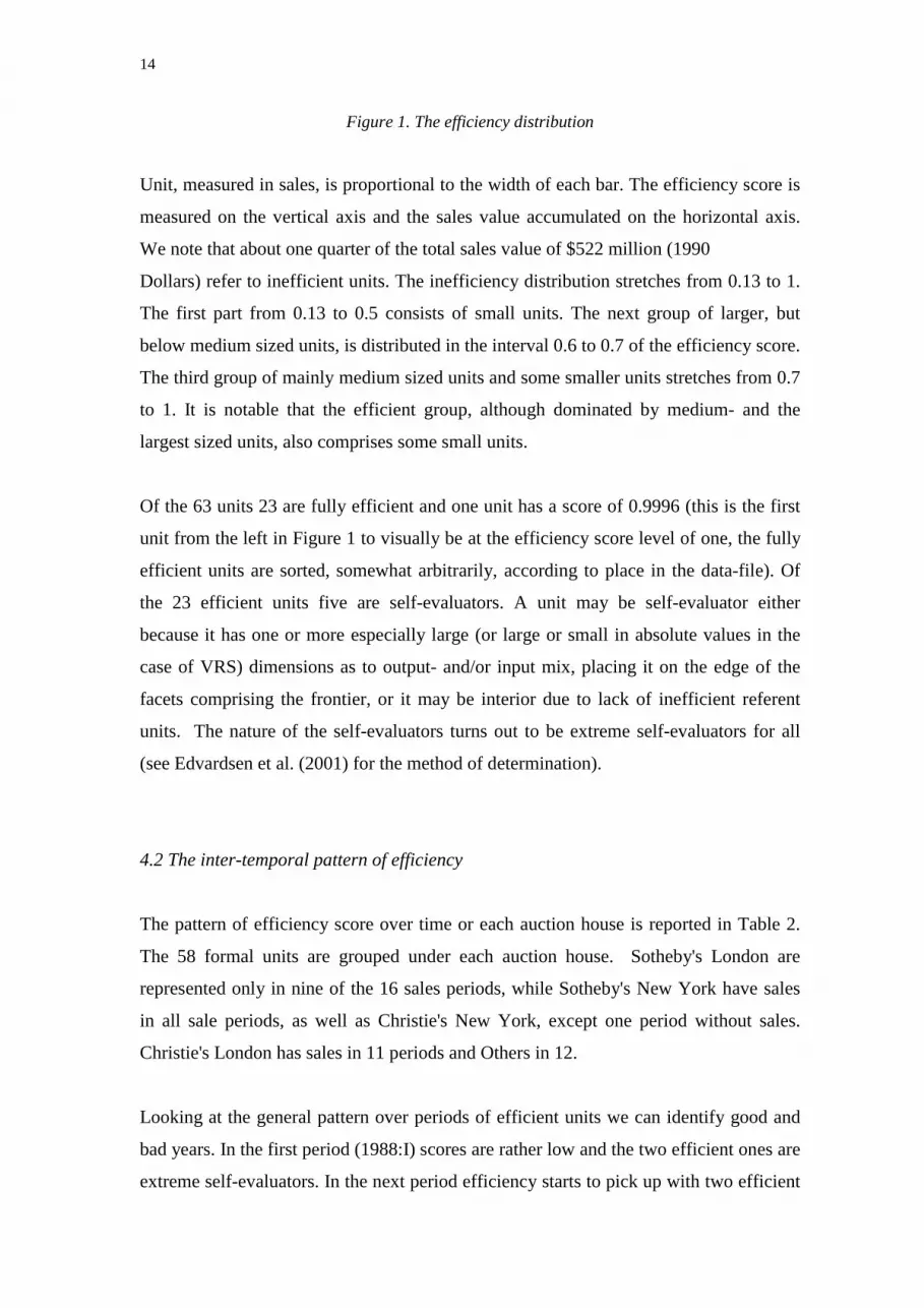
506 0.0562 0.0886 0.0300 1.59 8* Not feasiblenecessarily be greater than (or equal to) one. A third measure of the importance is a pure

count of the number of times a peer is a referencing unit for inefficient units.

Table 3 sets out the peer index and also the super efficiency index and number of

occurrences as referencing unit for a comparison. The indexing of the units by a three-

digit number has the number for the auction house14 and the period number as indicated

in Table 2.15 Table 3 displays that five of the 23 efficient units (201, 204, 314, 501,504)

are self-evaluators, i.e. they are not peers for any inefficient unit. Removing these units

will consequently have no impact on the efficiency scores of any inefficient unit, their

Peer index values are zero. As mentioned earlier they are also extreme self-evaluators

in the sense that they belong to facets not being of full dimensions (in our case eight).

Of the 18 remaining real peers a few stands out as most influential in terms of the peer

index value, while most of the peers are so for very few inefficient units. The number of

occurrences is given in the last column.

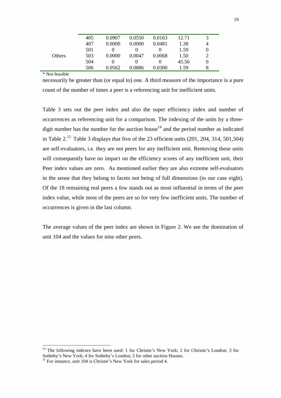
The average values of the peer index are shown in Figure 2. We see the domination of

unit 104 and the values for nine other peers.

14 The following indexes have been used: 1 for Christie’s New York; 2 for Christie’s London; 3 forSotheby’s New York; 4 for Sotheby’s London; 5 for other auction Houses.15 For instance, unit 104 is Christie’s New York for sales period 4.

20

Figure 2. The average peer index

Figure 3. Decomposition of the average peer indices

The decomposition of the average peer index in Figure 2 for all the peers in Table 3 is

illustrated in Figure 3. We see clearly the dominating position of unit 104 regarding

Period 3 paintings. Unit 106 dominates the Period 1 paintings, and units 104, 404 and

115 are on top for Period 2.

p g

0% 5% 10% 15% 20% 25%

102

104

105

106

111

Christie's New York 115

201

204

Christie's London 205

302

303

304

311

314

Sotheby's New York 315

403

404

405

Sotheby's London 407

501

503

504

Others 506

Y1Y2Y3

10424%

30212%

10611%404

8%

1158%

3046%

3116%

5066%

4055%

2054%

Rest10%

21

In Section 2.3 some general insights as to the nature of peers in the categorical model of

the type applied here to estimate the efficiency of auction houses was referred to. The

results imply that since types are identical both for inputs and outputs, the number of

positive variables exhibited by the peers must be matched with reference to both inputs

and outputs. Hence, an inefficient unit will be compared with peers having the same or

less types both of inputs and outputs, and all types of the inefficient unit must be

represented in the set of peers. Let us give some examples. Consider a unit of analysis

(an auction house for a specific sale period) only selling paintings from the first Picasso

period: this will only be compared with units selling period 1 paintings, while a unit of

analysis selling paintings from all three periods may be compared with units selling

from all periods, two periods or one period. From Table 3 we have that unit 106 has the

highest peer index value for Picasso Period 1 paintings, but sales of this unit consist of

only one painting from Picasso Period 2. Further, we see from Table 3 that the unit is

peer for three units. All these units are selling Period 2 paintings, but only one period 2

only, another is selling both periods 2 and 3 and the third one is selling all type of

paintings. We have that the peer index for unit 106 for Period 2 paintings is only a third

of the value for Period 1, and also slightly lower than for Period 3 paintings. The size of

weights and the volume of sales for the inefficient units explain the numbers within

each period of paintings.

Units 104 and 302 are the only peers among the five most influential for all types of

paintings. Unit 104 is the most influential peer for both Period 2 and Period 3 paintings,

although it represents only two Period 3 painting itself, Buste de femme, and Plant de

tomate. As explained above unit 106 is by far the most influential peer for Period 1

paintings, although it has sales of only Period 2 paintings, La dormeuse au miroir. Also

units 506 and 311 have sales from only one period, while units 302, 404, and 115 have

sales from two periods, and units 304 and 404 have sales from all three periods of

paintings. Thus the linkage effects through a painting period in common are strong. This

may not be so unreasonable because since the auction house is the unit, if it is efficient

in selling one type of painting it should also be efficient in selling other periods. It is

interesting that among the five most influential units for each paintings period we have

six from the first boom period, and one from the last boom period. The only auction

house not to be represented among the five for each painting period is Christie’s

London, Christie’s New York having three of the most influential from each boom

22

period, Sotheby’s New York having two from the boom period and one from and

remarkably having one from the weak market period, while Sotheby’s London and

Others have one each from the first boom period.

Regarding the Period 3 paintings, the one dominating peer, unit 104, Christie’s New

York for the year 1989:II, has an index value of 0.46, meaning that somewhat less than

half of the total weighted potential improvement in auction values are due to the

inefficient units having unit 104 as a peer. This is the maximal value for all types of

paintings. We see that the peer index values for the other two working periods for unit

104 are much smaller. The count index for this unit is the maximal almost the double of

the peer with the second highest, unit 302. This unit has the second highest peer index

value for Period 3 paintings, but is not so highly ranked for the two other painting

periods. This lack of discrimination using the count number as to type of painting is also

the case for the units with the third and fourth highest count numbers, showing the

limitation with this indicator of importance.

The super efficiency index is even of less use compared with the peer index values as

regards importance as role models. We see from Table 3 that unit 504 has by far the

highest super-efficiency index of 45.6, meaning that the proportional reference point on

the frontier without unit 504 has a sales value of (1/45.6) or only 2.2% of that observed

for unit 504. This seems highly suspect. However, unit 506 is a self-evaluator! The

second highest super efficiency index is for unit 302, which has high peer index values,

but, again, the third highest values is for unit 405 with modest values of the peer index.

There seems to be a poor correlation between the value of the super efficiency score and

the importance of the peer in terms of a peer being a referent for many inefficient units.

The super efficiency index seems to be of more value as a guide to a sensitivity check

on the shape of the frontier.

4.5 The ranking of an auction house

Our unit in the DEA program is an auction house in a specific sales period. So for each

auction house there are at maximum 16 efficiency scores calculated relative to the inter-

temporal frontier, as shown in Table 1. One way of utilising this information is to

construct hypothetical sales values for inefficient units by employing the efficiency

scores. For each type of painting we can compare the sales performance over all the

MmAap

E

pPI T

iami

ai

T

iami

am ,..,1and,..,1 ,1

1

1 ===�

�

=

=

23

auction periods for each auction house by forming the ratio of actual sales values over

calculated efficient sales values. We can then construct two types of performance

indicators for auction houses. An auction house performance indicator, PIam for a

specific type of painting, and an action house overall performance indicator, PIa, taking

into account all types of paintings. The formal definitions of the performance indicators

are:

(4)

(5)

Table 4. Auction house period- and overall performance indicators(Sensitivity runs results without unit 104 in parenthesis)

Auction Houses First Period(1881-1915)

Second Period(1916-1943)

Third Period(1944-1973)

OverallPerformance

Christie’s NewYork

0.91 (0.92) 0.77 (0.79) 0.70 (0.73) 0.79 (0.82)

Christie’s London 1 (1) 0.97 (0.98) 0.81 (0.98) 0.88 (0.98)Sotheby’s NewYork

1.00 (1.00) 0.88 (0.88) 0.83 (0.87) 0.92 (0.93)

Sotheby’s London 0.83 (0.83) 0.91 (0.93) 0.72 (0.82) 0.82 (0.87)Others 1.00 (1.00) 0.84 (0.86) 0.52 (0.80) 0.86 (0.94)

The potential sales of each type painting, m, are calculated using the sales period

efficiency scores for each auction house, a. The performance indicators will be between

0 and 1. The results are set out in Table 4.

Note that not only the efficiency scores, but also the volume of sales count when

constructing the performance indicators. An auction house may have a low efficiency

score for a period, as for Christie's New York 1991:II and Sotheby's New York 1992:I,

but this may not influence the performance index much of the sales involved are small.

Aap

E

pPI T

i

M

mami

ai

T

i

M

mami

a ,..,1 ,1

1 1

1 1 ==��

��

= =

= =

24

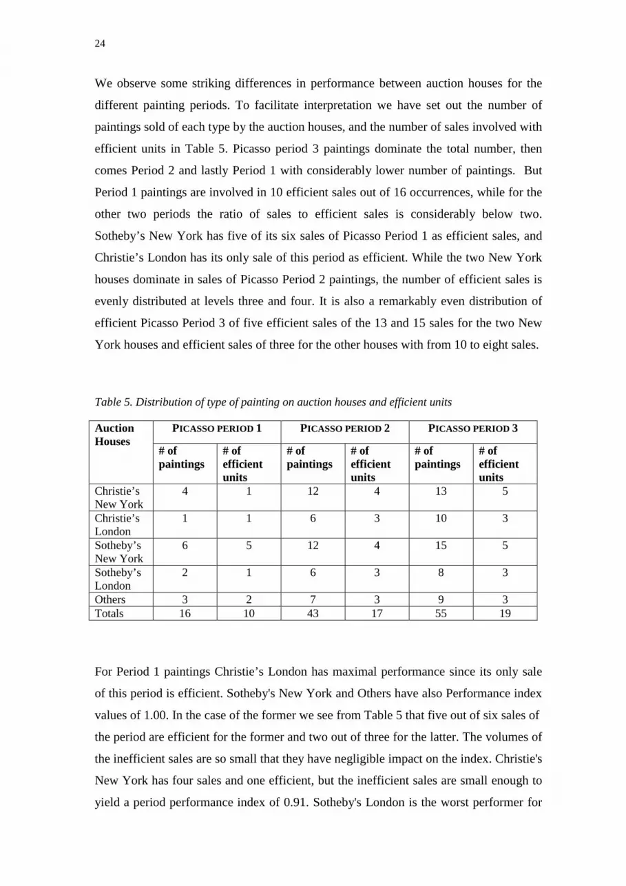
We observe some striking differences in performance between auction houses for the

different painting periods. To facilitate interpretation we have set out the number of

paintings sold of each type by the auction houses, and the number of sales involved with

efficient units in Table 5. Picasso period 3 paintings dominate the total number, then

comes Period 2 and lastly Period 1 with considerably lower number of paintings. But

Period 1 paintings are involved in 10 efficient sales out of 16 occurrences, while for the

other two periods the ratio of sales to efficient sales is considerably below two.

Sotheby’s New York has five of its six sales of Picasso Period 1 as efficient sales, and

Christie’s London has its only sale of this period as efficient. While the two New York

houses dominate in sales of Picasso Period 2 paintings, the number of efficient sales is

evenly distributed at levels three and four. It is also a remarkably even distribution of

efficient Picasso Period 3 of five efficient sales of the 13 and 15 sales for the two New

York houses and efficient sales of three for the other houses with from 10 to eight sales.

Table 5. Distribution of type of painting on auction houses and efficient units

PICASSO PERIOD 1 PICASSO PERIOD 2 PICASSO PERIOD 3AuctionHouses

# ofpaintings

# ofefficientunits

# ofpaintings

# ofefficientunits

# ofpaintings

# ofefficientunits

Christie’sNew York

4 1 12 4 13 5

Christie’sLondon

1 1 6 3 10 3

Sotheby’sNew York

6 5 12 4 15 5

Sotheby’sLondon

2 1 6 3 8 3

Others 3 2 7 3 9 3Totals 16 10 43 17 55 19

For Period 1 paintings Christie’s London has maximal performance since its only sale

of this period is efficient. Sotheby's New York and Others have also Performance index

values of 1.00. In the case of the former we see from Table 5 that five out of six sales of

the period are efficient for the former and two out of three for the latter. The volumes of

the inefficient sales are so small that they have negligible impact on the index. Christie's

New York has four sales and one efficient, but the inefficient sales are small enough to

yield a period performance index of 0.91. Sotheby's London is the worst performer for

25

this period, although it has one of its two sales as efficient. The inefficient sales have a

sufficiently large volume to yield this result.

With reference to the working period 2 production, Christie's London is outstanding in a

league of its own with almost no efficiency loss at all with a performance index of 0.97.

It has sales of the working period 2 paintings in six of the 11 sales periods, and for three

of these periods the efficiency scores are one. When the sales of Christie's London are

inefficient, the sales volumes are quite small. The New York branch of Christie's is

doing worst for Period 2 paintings. Of its 12 sales of this period four are efficient. This

is the same structure as Sotheby's New York, having a higher performance index. The

volumes of inefficient and efficient sales determine the outcome of the performance

index. Sotheby's London has the same structure as Christie's London, but again it has

another mix of volumes as to inefficient and efficient sales.

As regards Period 3 paintings the performance indicators are low in general and the two

best houses, Sotheby's New York and Christie's London being almost equal and far in

front of the others. This is the type of painting having positive sales in most of the

periods. According to Table 3, in the sale period 4 (1989:II) Christie’s New York is the

dominating peer, having sales only of a Period 3 painting. Notice that a dominating peer

will also “punish” other sales performances for the same auction house. The index for

Christie’s New York is lower than for all the other houses with the exception of the

group Others. The particularly bad performance of Others is due to the efficiency score

being one only in three of the nine sales periods when the working period 3 paintings

are sold. The auction 104 of Christie’s New York is the peer for six of the eight

inefficient sales of Others, five of seven for Christie's London, three of five for

Sotheby's London, and six of 10 for Sotheby's New York. The influence of the

dominating peer depends both on the efficiency scores and the volumes of sale.

When aggregating to the overall performance index Sotheby's New York appears as the

most efficient house over all Picasso periods and sales periods. Christie's London

follows then, and Others auction house follows as number three. Sotheby's London and

Christie’s New York are at the bottom. The placing of the former reflects the

performances for Period 1 and Period 3 paintings, while the bottom ranking for the

latter stems from the weak performance for Period 2 and Period 3. Notice that Others is

26

not doing as badly as expected from the Period 2 and period 3 results. This is explained

by the fact that one of its Period 1 efficient sales involve the most expensive picture in

the data set sold for $48 millions (see Table 1). The volume for this period outweighs

the low performance indicators for the other periods.

4.6 Sensitivity results

Both the peer index values and the count of number of times a peer appears as a

referencing unit point to unit 104, Christie's New York for sales period 1989:II, as a key

influential unit. However, none of its continuous data seem suspect. It happens to be

located centrally in the data set. Inspecting the super efficiency score this is 2.97,

meaning that removing this unit from the data set and then calculating the efficiency

measure against this new frontier implies that unit 104 has a sales value 2.97 times the

calculated sales value of the reference point on the frontier, or that the reference point

on the frontier has a sales values of only (1/2.97) or 33.7 per cent of unit 104’s sales

value. So among similar units unit 104 stands out. Moreover, unit 104 is peer for 23

inefficient unit, almost twice as many as the peer with the second highest counts. Such a

situation calls for an investigation of the sensitivity of the results to a change in the

observation. As already mentioned we do not suspect any incorrect data, but it may be

unique circumstances concerning the sale, and it is also of a general interest to

investigate the stability or robustness of the results. The results for inefficient units with

a high share of the working period 3 paintings may be significant, but not necessarily so

for inefficient units with highest shares of the two other period paintings. The

pinpointing of unit 104 highlights both the weakness and strength of the DEA method:

the weakness is the dependence of the results on few observations, and the strength is

that we have identified the one single unit that drives part of the results and that must be

checked.

The sensitivity analysis is performed simply by running the DEA model on the data set

without unit 104. All inefficient units will then experience either no change in efficiency

score or an increased efficiency score. Of the 40 inefficient units in the main analysis 23

units got an increase in the efficiency score, and of these five became fully efficient.

The changes range from very minor (0.004) to quite large (0.58). The units with the

highest changes where previously located among the small inefficient units in the first

27

tail of the efficiency distribution shown in Figure 1 (with the exception of two units).

The arithmetic average (unweighted) of the efficiency score increased from 0.69 to

0.79.

As regards the impact on the peer index values none of the new fully efficient units

make it up among the five most influential. All the four units ranked behind 104

increase their share with factors around 0.04, and otherwise change in peer index values

are small for the units moving up concerning Period 2 paintings, and there are almost no

changes in peer index values for Period 1 paintings.

Looking at the auction houses Christie's London benefits by increasing five of its 11

inefficient units with numbers in the range of 0.39-0.57, getting two fully efficient ones

more. Although Sotheby's New York gets three new fully efficient units only one

increase is substantial (0.54). Sotheby's London has no new fully efficient ones and only

one substantial increase, too (0.58), while Others experience substantial increases for six

of its 12 inefficient units, but without getting more fully efficient ones.

These changes explain the new pattern of performance indicators given within

parenthesis in Table 4. We have that there are almost no changes for Period 1 paintings,

and only minor adjustments for Period 2 paintings of magnitude 0.02 index points. The

large changes all come for Period 3 paintings. We see that Others have a substantial

increase of 0.28, and Christie’s London increases with 0.17. The changes for the last

period are enough to change the ordering of the total performance indicators. Christie’s

London moves to first position and Others move up to second position. The original

leader, Sotheby’s New York, is relegated to third position. Sotheby’s London and

Christie’s New York remain in fourth and fifth position, respectively.

5. Concluding remarks

Although there is an increasing emphasis on performance of investment in paintings, the

role of auction houses has not been studied so much in the economic literature. Previous

works applying hedonic price technique have found no conclusive result about the most

28

efficient auction house, but in these studies the object of art has been the unit, and

influence of auction houses is analysed by testing whether auction house impact on

price is significant or not within a framework of central tendencies. In order to focus on

auction houses as a unit we have applied a benchmarking technique, DEA, developed

for efficiency studies. The assumed production process is a little special: the inputs are

the physical characteristics of Picasso paintings, and the outputs are the auction prices.

Categorical and continuous variables are used as inputs, and auction prices as outputs.

We cannot, of course, capture all relevant information about paintings simply by type of

period and area of painting. However, these are the variables found significant and used

in studies of auction prices using hedonic regressions.

We have developed a model with mixed categorical and continuous variables most

suitable for art objects markets not used before in the efficiency literature. New light is

shed on the issue of categorical variables in DEA models by interpreting them as

different types of inputs and/or outputs. The inter-linkages between categorical

variables turned out to be important for the empirical findings.

A novel construct of the paper is Performance indicators giving an insight into auction

house differences impossible to obtain using hedonic price regressions. If you plan to

sell your Picasso you would prefer the auction house with the best performance to

handle your sales, but if you want to do a bargaining buying, you should go to the

auction house with the lowest value of the performance index.

The type of model developed may also be applied to other institutions or markets, where

the unit in question use physical assets of various types to produce a financial result, e.g.

financial market units like stock broker firms, pension funds, etc.

References

Afriat, S. (1972): “Efficiency estimation of production functions,” International

Economic Review 13(3), 568-598.

29

Agnello, R. J. and R.K. Pierce (1999): “Investment Returns and Risk for Art:

Evidence from Auctions of American Paintings (1971-1996)”, Working Paper 99/03

University of Delaware.

Aigner, D. J. and S.F. Chu (1968): “On estimating the industry production function,”

American Economic Review 58, 226-239.

Aigner, D. J., C.A.K. Lovell and P. Schmidt (1977): “Formulation and Estimation of

Stochastic Frontier Production Function Models,” Journal of Econometrics 6(1), 21-

37.

Andersen, P. and N. C. Petersen (1993): “A procedure for ranking efficient units in

Data Envelopment Analysis”, Management Science 39, 1261-1264.

Anderson, R.C. (1974): "Paintings as Investment", Economic Inquiry 12,13-26.

Banker, R. D. and R. C. Morey (1986): "The use of categorical variables in Data

Envelopment Analysis", Management Science 32(12), 1613-1627.

Boles, J. N. (1967): “Efficiency Squared—Efficient computation of Efficiency

Indexes,” Western Farm Economic Association, Proceedings 1966, Pullman,

Washington, 137-142.

Boles, J. N. (1971): The 1130 Farrell Efficiency System – Multiple Products, Multiple

Factors, Giannini Foundation of Agricultural Economics, February 1971.

Buelens, N. and V. Ginsurgh (1993): “Revisiting Baumol’s ‘art as floating crap

game’,” European Economic Review 37, 1351-1371.

Candela, G. and E. Scorcu (1997): “A Price Index for Art Market Auctions. An

application to the Italian Market of Modern and Contemporary Oil Paintings”,

Journal of Cultural Economics 21(3), 175-196.

30

Chanel, O., L.A. Gérard-Varet and V. Ginsurgh (1996): “The Relevance of Hedonic

Price Indices”, Journal of Cultural Economics 20, 1-24.

Charnes, A., W.W. Cooper and E. Rhodes (1978): “Measuring the efficiency of

decision making units,” European Journal of Operational Research 2, 429-444.

Charnes, A., W. W. Cooper, A. Y. Lewin and L. M. Seiford (eds.): Data Envelopment

Analysis: Theory, Methodology, and Applications, Boston/Dordrecht/London: Kluwer

Academic Publishers, 1994, Section 3.3 Categorical inputs and outputs, 52-54.

Combris, P., S. Lecocq and M. Visser (1997): “Estimation of a hedonic price equation

for Bordeaux wine: does quality matter?” The Economic Journal 107, 390-402.

Czujack, C. (1997): “Picasso paintings at auction, 1963-1994”, Journal of Cultural

Economics 21, 229-247.

Edvardsen, D. F., F. R. Førsund, and S. A.C. Kittelsen (2001): “Far out or alone in the

crowd: determining the nature of self-evaluators in DEA”, Working Paper

(forthcoming) from the Frisch Centre, Oslo, Norway.

Farrell, M. J. (1957): “The measurement of productive efficiency”, Journal of the

Royal Statistical Society, Series A, 120 (III), 253-281.

Färe, R., S. Grosskopf, and R.R. Russell (eds.) (1998): Index Numbers: Essays in

Honour of Sten Malmquist, Boston/London/Dordrecht: Kluwer Academic Publishers.

Frey, B.S. and W.W. Pommerehene (1989): Muses and Markets; Explorations in the

Economics of the Arts, Oxford: Basil Blackwell.

Førsund, F. R. (2001): “Categorical variables in DEA”, Working Paper 6/01, ICER,

Turin, Italy.

31

Førsund, F. R. and N. Sarafoglou (2000): “On The Origins of Data Envelopment

Analysis” Memorandum 24/2000 from the Department of Economics, University of

Oslo.

Griliches, Z. (1961): “Hedonic price indexes for automobiles: an econometric analysis

of quality change”, in The Price Statistics of the Federal Government, New York:

Columbia University Press.

Griliches, Z. (1990): “Hedonic Price Indexes and the Measurement of Capital and

Productivity”, in Ernst. R. and Triplett. J.E. (eds.), Fifty Years of Economic

Measurement, Chicago: University of Chicago and NBER, 185-202.

Kamakura, W. A. (1988): "A note on the use of categorical variables in Data

Envelopment Analysis", Management Science 34(10), 1273-1276.

Locatelli-Biey, M. and R. Zanola (2001): “The market for sculptures: an adjacent year

regression index”, Journal of Cultural Economics (forthcoming).

Meeusen, W. and J. van den Broeck (1977): “Efficiency Estimation from Cobb-

Douglas Production Functions with Composed Errors,” International Economic

Review 18, 435-444.

Pesando, J.E. (1993): “Art as an investment: The market for modern prints”,

American Economic Review 83, 1075-1089.

Renneboog, L. and T. Van Houtte (2000): “From Realism to Surrealism: Investing in

Belgian Art”, Cahiers-Economiques-de-Bruxelles 165, 69-106.

Rosen, S. (1974): “Hedonic Prices and Implicit Markets: Product Differentiation in

Pure Competition”, Journal of Political Economy 82, 34-55.

Seiford, L. M. (1996): “Data Envelopment Analysis: The Evolution of the State of the

Art (1978-1995),” Journal of Productivity Analysis 7 (2/3), 99-137.

32

Torgersen, A. M., F. R. Førsund, and S. A. C. Kittelsen (1996): “Slack-adjusted

efficiency measures and ranking of efficient units”, Journal of Productivity Analysis,

7(4), 379-398.

Tulkens, H. and P. van den Eeckaut (1995): “Non-parametric efficiency, progress, and

regress measures for panel data: methodological aspects”, European Journal of

Operational Research 80, 474-499.