Embed Size (px)
Citation preview
Southern Flow Corridor baseline effectiveness monitoring: 2014
February 29, 2016 (revision 2, 12/27/2016) Prepared by: Laura A. Brown1, Michael J. Ewald 1, Laura S. Brophy1, and Stan van de Wetering2 1Estuary Technical Group, Institute for Applied Ecology, Corvallis, Oregon
2Confederated Tribes of Siletz Indians of Oregon, Siletz, Oregon
Prepared for:
Tillamook County, Tillamook, Oregon
Tillamook SFC Baseline Effectiveness Monitoring, 2014 Rev. 2, 12/27/16, P. 2 of 215
Southern Flow Corridor baseline effectiveness monitoring: 2014
Authors: Laura A. Brown1, Michael J. Ewald1, Laura S. Brophy1, and Stan van de Wetering2 Institutional affiliations for authors at the time of this project: 1Estuary Technical Group, Institute for Applied Ecology, Corvallis, Oregon 2Confederated Tribes of Siletz Indians, Siletz, Oregon Contact for data and further project details: Laura Brophy, Director, Estuary Technical Group, Institute for Applied Ecology, [email protected], (541) 286-8643 Changes in author affiliations since project completion:
• Laura Brown is now at the Confederated Tribes of Siletz Indians, Siletz, Oregon.
• Michael Ewald is now at Geomatics Research, Inc. Additional project team members and roles: Scott Bailey3: field data collection Dillon Blacketer4: field data collection Julie Brown5: field data collection Chris Janousek6: experimental design, field data collection Issac Kentta4: field data collection Susanna Pearlstein7: field data collection Erin Peck8: field data collection and carbon core analysis Robert Wheatcroft8: field data collection and carbon core analysis Institutional affiliations for additional project team members: 3 Tillamook Estuaries Partnership, Garibaldi, Oregon 4 Confederated Tribes of Siletz Indians, Siletz, Oregon 5 Quantum Spatial, Corvallis, Oregon 6 Department of Fisheries and Wildlife, Oregon State University, Corvallis, Oregon 7 U.S. Environmental Protection Agency, Corvallis, Oregon 8 College of Earth, Ocean, and Atmospheric Sciences, Oregon State University, Corvallis, Oregon Recommended citation: Brown, L.A., M.J. Ewald, L.S. Brophy, and S. van de Wetering. 2016. Southern Flow Corridor baseline effectiveness monitoring: 2014. Corvallis, Oregon: Estuary Technical Group, Institute for Applied Ecology. Prepared for Tillamook County, Oregon. Data availability: Data from this project are available from the Estuary Technical Group (Laura Brophy, contact information listed above).

Tillamook SFC Baseline Effectiveness Monitoring, 2014 Rev. 2, 12/27/16, P. 3 of 215
Revision history:
• 6/5/16, revision 1: corrected institutional affiliations for authors and project members; added clarifying details to Appendix F.
• 12/27/16, revision 2: corrected percent inundation values; added details on methods for calculating percent inundation. Added a key finding describing the undisturbed condition of high marsh vegetation at Dry Stocking Island and Goose Point. Revised Table 23 to show elevations of soil surface and water level sensor for each groundwater well installation.
Acknowledgments:
• We are grateful for the funding provided for this project by the National Oceanic and Atmospheric Administration, Oregon Watershed Enhancement Board, and U.S. Fish and Wildlife Service.
• We thank the U.S. Environmental Protection Agency, Coastal Ecology Branch, Newport, Oregon for its major contribution to this project through the loan of RTK-GPS and cryocore equipment.
• We thank the Oregon Department of Fish and Wildlife for their major contribution to this project through the loan of a boat.
• Many thanks to the volunteers who assisted with field data collection: Peter Idema, Danielle Aguilar, Greg Hublou.
• We are grateful to Wes Maffei for his expert advice on mosquito monitoring, and for mosquito identification.
• Thanks to Chad Allen for the loan of his all-terrain vehicle.
Tillamook SFC Baseline Effectiveness Monitoring, 2014 Rev. 2, 12/27/16, P. 4 of 215
Table of contents SUMMARY AND KEY FINDINGS ..................................................................................................................... 6
Key findings ............................................................................................................................................... 7
REPORT ORGANIZATION: RESTORATION AND MONITORING OBJECTIVES ................................................ 12
Effectiveness monitoring objectives and hypothesis ............................................................................. 12
Project timeline and design overview .................................................................................................... 13
Methods overview .................................................................................................................................. 15
Study sites ............................................................................................................................................... 15
Southern Flow Corridor (SFC) site ...................................................................................................... 15
Reference sites ................................................................................................................................... 17
General sample design ........................................................................................................................... 18
METHODS AND RESULTS BY MONITORING OBJECTIVE .............................................................................. 19
EM Objective 1: Vegetation .................................................................................................................... 19
Emergent and tidal wetland plant communities ................................................................................ 19
Plant community mapping ................................................................................................................. 40
EM Objective 2: Wetland physical conditions ........................................................................................ 45
Wetland surface elevation and water level ....................................................................................... 45
Channel water salinity and temperature ........................................................................................... 60
Groundwater levels ............................................................................................................................ 74
Soils .................................................................................................................................................... 82
Channel morphology .......................................................................................................................... 88
Sediment accretion and erosion ...................................................................................................... 114
Linked monitoring of biological and physical parameters ............................................................... 124
EM Objective 3: Fish use, prey resources, and habitat ........................................................................ 127
Fish distribution, abundance, and tidal migration ........................................................................... 127
Fish distribution and abundance ...................................................................................................... 127
Tidal migration ................................................................................................................................. 133
Prey resources (benthic macroinvertebrates) ................................................................................. 143
EM Objective 4: Flood attenuation ....................................................................................................... 149
EM Objective 5: Mosquito monitoring ................................................................................................. 149
Mosquito monitoring ....................................................................................................................... 149
CONCLUSIONS AND RECOMMENDATIONS ............................................................................................... 152
REFERENCES .............................................................................................................................................. 154
Appendix A. Maps ..................................................................................................................................... 161
Tillamook SFC Baseline Effectiveness Monitoring, 2014 Rev. 2, 12/27/16, P. 5 of 215
Appendix B. Additional figures .................................................................................................................. 186
Channel morphology ............................................................................................................................ 186
Multi-parameter ................................................................................................................................... 190
Appendix C. Additional tables ................................................................................................................... 198
Appendix D. Spatial data information ....................................................................................................... 206
Spatial reference system ...................................................................................................................... 206
GPS/GNSS methods .............................................................................................................................. 206
Spatial data accuracy ............................................................................................................................ 206
Feet / meters conversion ...................................................................................................................... 206
Appendix E. Plant community metrics across habitats ............................................................................. 207
Appendix F. Sediment accretion and erosion rates using sediment stake method ................................. 209
Appendix G. “Blue” carbon accumulation: Progress report ..................................................................... 214
“Blue” carbon accumulation overview ................................................................................................. 214
Project activities performed to date ................................................................................................ 214
Upcoming project activities ............................................................................................................. 214
Tillamook SFC Baseline Effectiveness Monitoring, 2014 Rev. 2, 12/27/16, P. 6 of 215
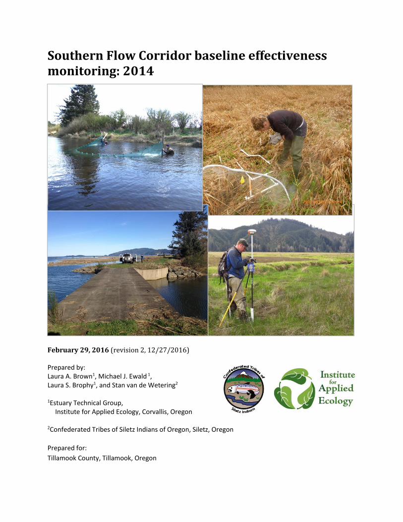
SUMMARY AND KEY FINDINGS Baseline effectiveness monitoring for the 210 ha (519 acre) Southern Flow Corridor (SFC) site and three nearby least-disturbed reference sites was conducted during October 2013 - May 2015 by the Estuary Technical Group (ETG) of the Institute for Applied Ecology and the Confederated Tribes of Siletz Indians (CTSI). Laura Brophy, ETG Director, led the monitoring of tidal hydrology, plant communities, groundwater, soils, mosquitoes, water temperature and salinity, and sediment accretion. Stan van de Wetering, Aquatic Programs Leader with CTSI, led the monitoring of fish use and macroinvertebrates. All team members collaborated on channel morphology monitoring, and on analyses of the linkages between physical and biological characteristics at the site. The SFC Effectiveness Monitoring Plan (Brophy and van de Wetering 2014) was peer-reviewed by the SFC Monitoring Advisory Committee prior to the beginning of baseline monitoring. Effectiveness monitoring was designed and implemented by ETG and CTSI to enable the evaluation of progress towards SFC project goals and improved ecological functions. Baseline monitoring provides data for comparison to post-project effectiveness monitoring, and baseline data can also be used to refine project design. As described in the SFC Effectiveness Monitoring Plan (Brophy and van de Wetering 2014), selection of monitoring parameters was based on a conceptual model of ecosystem function, and parameters selected were those likely to provide a clear picture of the outcome of the project in reference to the project goals. Field data was collected from the SFC site and three nearby least-disturbed reference sites. The three reference sites were Dry Stocking Island, Bay Marsh, and Goose Point. The main body of this report provides summaries, representative results, and interpretation. Further results are provided in the appendices, and additional data are available from lead authors. Since this is a baseline monitoring report, project results cannot yet be evaluated. Instead, this report highlights key differences between the SFC site and reference sites, demonstrating how past alterations of the SFC site have affected physical and biological conditions at the SFC site. During the baseline monitoring period, physical and biological conditions were noticeably different between the SFC site and reference sites for all metrics monitored. The majority of these differences were due to the lack of tidal influence at the SFC site, and the SFC site’s current and past agricultural use. Tidal reconnection and removal of flow barriers, as planned at the SFC site, are expected to produce a shift in biological and physical conditions towards reference conditions, though some conditions will change more rapidly than others – typical of restoration sites in general. Key findings are listed below.
Tillamook SFC Baseline Effectiveness Monitoring, 2014 Rev. 2, 12/27/16, P. 7 of 215
Key findings
To jump to further details about each key finding, click on the underlined hyperlink. Key findings for emergent and tidal wetland plant communities:
• Overall, native species cover and species richness were significantly lower at the SFC site compared to the reference sites.
• Reed canarygrass was one of the dominant species at the SFC site in every zone except Nolan crop and Nolan grazed.
• Species richness increased with elevation at the SFC site and reference sites. • Emergent tidal wetlands at the reference sites were dominated by native plant species typical of
Oregon’s outer coast tidal marshes, such as Lyngbye’s sedge and tufted hairgrass. • Woody species (primarily shrubs) were found in the North and Middle zones, likely due to a lack
of grazing and pasture maintenance in those zones in recent years. • Non-native species were almost completely absent from the tufted hairgrass high marsh at Dry
Stocking Island and Goose Point, making these two sites particularly valuable as examples of least-disturbed high marsh for the Oregon outer coast.
Key findings for plant community mapping: • Plant communities at the SFC site were dominated by non-native species. Non-native dominated
communities occupied 111.6 ha (60.6% of the site), while native-dominated communities occupied only 53.6 ha (29%) of the site.
• Reference sites were almost exclusively occupied by native-dominated plant communities. • Many of the non-native and native dominants at the SFC site are likely to die back after
restoration of brackish tidal flows. • Salinity tolerance varies among woody dominants in forested and shrub wetlands at the SFC
site, but the post-restoration combination of increased inundation and salinity will likely lead to dieback of many of the woody plants on the site.
• A number of current and potential invasive species were found at the SFC site; most are likely to be greatly reduced by the restored tidal inundation and salinity. Guidance is provided for each species.
Key findings for wetland surface elevation and water level:
• Based on nearby reference sites, the SFC site was probably high marsh prior to European settlement and conversion to agricultural use.
• Average wetland surface elevation was around 2.05 m NAVD88 at the SFC site and 2.68 m NAVD88 at the high marsh reference sites, indicating around 62 cm of subsidence occurred after conversion to agricultural use. Estimated subsidence varied between 37 cm and 78 cm across the site and appeared to be related to land use history, with currently cropped areas having the greatest estimated subsidence.
• High tide datums at study sites were similar to the NOAA tide station at Garibaldi (MHHW ~2.4 m, MHW ~2.2 m NAVD88), but low tide datums were much higher near SFC (MLLW 0.5 m, MLW 0.8 m NAVD88 at our Dry Stocking Island gauge, compared to -0.124 m at Garibaldi). This results reflects the strong fluvial (riverine) component to the tidal inundation regime at the SFC site.
• The strong fluvial component of the tide regime was also illustrated by tidal lag times. High tide (marine-driven) peaks near the SFC site lagged only 10-20 minutes behind the NOAA Garibaldi station, but lower low tides (river-driven) lagged around 2 hours behind the Garibaldi gauge.
• Daily maximum water levels were significantly lower at the SFC site compared to the reference sites, due to dikes and tide gates blocking tidal influence.
Tillamook SFC Baseline Effectiveness Monitoring, 2014 Rev. 2, 12/27/16, P. 8 of 215
• During the summer dry season, plots at the SFC site did not inundate; they inundated only during the winter wet season. Fluvial input generally elevated water levels throughout the study area in winter.
• At the reference sites, all but one of the study plots were inundated regularly during the summer dry season. The single reference plot that did not inundate in summer inundated due to tidal forces during other seasons.
Key findings for channel water salinity and temperature:
• Daily maximum channel water salinity was significantly lower at the SFC site compared to reference sites during all seasons, due to dikes and tide gates blocking tidal influence from the SFC site.
• Nolan Slough had the highest salinity in the winter of all loggers at the SFC site, likely due to its proximity to an observed leaky tide gate.
• At the reference sites, winter salinities were higher than early spring salinities.
• Salinities at reference sites decreased with increasing distance from the mouth of Tillamook Bay.
• Daily maximum channel water temperature was significantly higher at the SFC site compared to the reference sites during all seasons, except winter.
Key findings for groundwater levels:
• Daily maximum groundwater levels were significantly lower at the SFC site compared to reference sites, due to the site’s drainage infrastructure (dike/tide gate system) and the resulting elimination of tidal influence at the SFC site.
• The SFC site is a seasonal wetland; winter and summer groundwater levels averaged 0.1 m and 0.6 m below the soil surface, respectively.
• Based on groundwater levels, South no crop was the wettest zone within the SFC site (likely due to its low elevation), and Nolan ungrazed was the driest zone (likely due to its high elevation).
Key findings for soils:
• Soil pH and soil salinity were both significantly lower at the SFC site when compared to nearby reference sites.
• Soil pH increased significantly as elevation decreased at the SFC site, though not at the reference sites.
Key findings for sediment accretion and erosion:
• Sediment accretion rates were not statistically different between the SFC site and nearby reference sites.
• Sediment accretion rates were not significantly related to elevation at the SFC site or reference sites.
• Accretion rates found in this study were higher than those found by our team in the Siuslaw River Estuary, and in several other studies.
• Flooding of the SFC site likely brings in sediments, and recurring flooding within the site likely redistributes sediment across the site, leading to high rates of accretion.
• Tillamook Bay historically has had high rates of sediment deposition, likely leading to the high rates of accretion at the study sites compared to other estuaries.
Key findings for channel morphology:
• Very thick layers of fine sediment have accumulated behind tide gates within the SFC site. The fine sediments probably have a high component of organic matter from aquatic plants, such as the abundant parrotfeather milfoil. These fine sediments will likely be exported and redistributed after project implementation.
Tillamook SFC Baseline Effectiveness Monitoring, 2014 Rev. 2, 12/27/16, P. 9 of 215
• The fine sediment surface showed a lower gradient and less variable elevation compared to the firm channel bottom beneath the fine sediment. This reflects the relatively stable water levels inside the site, compared to the water level fluctuations that would occur if tidal barriers (dikes and tide gates) were not in place.
• Channel depth to sediment surface was similar between the SFC site and reference sites, though when fine sediment depth was considered with channel depth, channels were deeper at the SFC site. This suggests channels may have been excavated and fine sediments may have accumulated within the channels. This interpretation was supported by channel bottom elevation and flowpath elevation as well.
• Bank slopes were lower and channel width-to-depth ratios were higher at the SFC site when compared to reference sites, likely as a result of oxidization, machinery use, and grazing.
• Similar patterns in bank slope and channel width-to-depth ratios have been found across the Oregon coast.
• Channels were wider at the SFC site compared to reference sites, likely due to site area and alterations.
Key findings for linkages between biological and physical parameters:
• Differences in plant communities between the SFC site and reference sites were associated with differing elevation, soil salinity, and soil pH.
• Species richness at the reference sites significantly increased with elevation.
Key findings for fish distribution and abundance:
• Because the SFC project is nested between the confluence of three rivers and is adjacent to the broad shallow delta plain in the southern portion of Tillamook Bay, resulting salinity, temperature and flow patterns make this area, relative to the full watershed, optimal habitat for juvenile salmonids as well as other estuarine dependent species.
• The fish community was predominantly composed of age-0 and age-1 Coho (Oncorhynchus kisutch), age-0 Chum (Oncorhynchus keta), age-0 Chinook (Oncorhynchus tshawytscha), and multiple age classes of Shiner perch (Cymatogaster aggregata), Three-spined stickleback (Gasterosteus aculeatus), Pacific Staghorn sculpin (Leptocottus armatus), Prickly sculpin (Cottus asper), and Starry flounder (Platichthys stellatus).
• Species distributions were affected by seasonality (shifts in stream flow, stream temperature and salinity) and habitat access (presence/absence of migration barriers - tide gates).
• Age-0 salmonids were more common early in the year when flows were higher, and stream temperatures and salinities were lower.
• Shiner perch and Three-spined-stickleback were less common early in the year and more common later in the year when stream flows were lower and temperatures and salinities were higher.
• Pacific Staghorn sculpin were more evenly distributed across all sampling months.
• With the SFC habitats Three-spined stickleback were dominant in the catch at all locations while Coho were dominant at a single location.
• Within reference habitats, age-0 Coho, Chum, and Chinook, were well distributed as were Pacific Staghorn sculpin, Prickly sculpin, Three spined-stickleback, and Shiner Perch. Age-1 Coho were sporadically distributed across the reference locations.
• Within the SFC habitats age-0 Chum, age-0 and age-1+ Starry flounder, age-0 Shiner perch, and age-1+ Cutthroat trout were absent during all sample months while a total of three age-0 Chinook, and one age-1 Shiner perch were observed.
Tillamook SFC Baseline Effectiveness Monitoring, 2014 Rev. 2, 12/27/16, P. 10 of 215
Key findings for tidal migration:
• Fish use in the study area was high with over 70,000 fish observed during six sampling periods.
• Net movement for age-0 salmonids was lower at all SFC locations when compared to their adjacent reference location.
• Migration behavior of age-0 salmonids at SFC locations was different from that of the river reference locations in that the fish completed an upstream and downstream migration within the immediate distance of the tide pipe.
• Migration behavior of age-0 salmonids at SFC locations was different from that of the river reference locations in that many of the fish remained within the immediate sampling habitat and fed on drifting prey.
• As depth and size of the SFC tide pipe headwater pool increased, more fish were observed migrating.
• Limited to no daily tidal migration of Chinook, Chum, Pacific Staghorn sculpin, Prickly sculpin, Shiner perch, and Starry flounder occurred at the SFC locations.
• We concluded that fish observed migrating at the SFC locations were predominantly rearing within the tide pipe itself, the tide pipe headwater pool, or the pool habitat immediately upstream of the tide pipe (few tens of meters) and not completing migrations between SFC and reference habitats.
Key findings for prey resources (benthic macroinvertebrates):
• Measures of diversity were greater for the SFC locations than at the mainstem river reference locations.
• There were significant differences in diversity both among SFC locations and among reference locations.
• Summed multispecies abundance values were lower for the SFC locations than for the reference locations.
• The most abundant taxa at SFC were chironomids, copepods, isopods, oligochaetes and hydrobiidae. Of these abundant taxa, chironomids, hydrobiidae and oligochaetes had the broadest distribution.
• Reference location abundance values were dominated by amphipods, copepods and chironomids.
• Invasive New Zealand mudsnails were found in samples from the NW Ditch sample site, but not at other sample locations.
• Although the invasive New Zealand mudsnails is increasing in its distribution across the eastern Pacific coast, we suggest the potential for expansion of this species within the SFC site post-restoration is limited.
• Results for the benthic community at the SFC site were similar to our observation at other Oregon estuarine diked wetlands.
Key findings for mosquito monitoring:
• Mosquito larvae counts peaked at the end of April, while adult mosquito counts peaked in the beginning of July.
• Culex tarsalis was the mosquito species counted most frequently at the SFC site.
• The salt marsh mosquito, Aedes dorsalis, a species that created problems at the Ni-les’tun restoration site (Bandon Marsh NWR), was not captured at the SFC site. It may, however, be present at adjacent reference sites (not monitored due to funding limitations).
• After project implementation, the majority of the SFC site will be tidally inundated on a daily basis, conditions which do not constitute preferred habitat for the salt marsh mosquito.

Tillamook SFC Baseline Effectiveness Monitoring, 2014 Rev. 2, 12/27/16, P. 11 of 215
Key findings for “blue” carbon study:
• Field work for the blue carbon study was completed in April 2015. Laboratory analysis of samples is currently underway and completion is expected during late winter to spring 2016. Results of the blue carbon study will be included in project reporting at the end of 2016.
Recommendations:
• During project implementation, monitoring infrastructure (particularly accretion plots and groundwater wells) should be protected from damage and disturbance. If accretion plots are disturbed, comparisons of accretion rates before and after project implementation will not be possible.
• Post-project effectiveness monitoring should follow the recommendations and methods presented in the SFC Effectiveness Monitoring Plan (Brophy and van de Wetering 2014). Continuation of these methods, which were used during the baseline study, will allow comparisons that are necessary for determination of project effectiveness.
• Post-implementation monitoring should address performance criteria, as recommended in the project’s Environmental Impact Statement (http://southernfloweis.org/).
• Mosquito monitoring is recommended for Year 1 and Year 2 after project implementation.
• Restoration design and monitoring recommendations resulting from this study have been provided by our team during formal and informal design review meetings and phone calls, and have been contributed to documents such as the SFC Baseline Documentation Report and fish salvage recommendations.
• Recommendations resulting from this study are also being used to guide monitoring, design and evaluation of project effectiveness at numerous other tidal wetland restoration sites in Oregon and the Pacific Northwest.
Tillamook SFC Baseline Effectiveness Monitoring, 2014 Rev. 2, 12/27/16, P. 12 of 215
REPORT ORGANIZATION: RESTORATION AND MONITORING OBJECTIVES This report is organized by the effectiveness monitoring objectives listed below. Monitoring objectives are found in the SFC Effectiveness Monitoring Plan (Brophy and van de Wetering 2014). Each monitoring objective is addressed by monitoring a variety of parameters. Effectiveness monitoring was designed to help determine whether the project’s goals are being met. Goals, as stated in the Tillamook County’s proposal to the NOAA Restoration Center (Tillamook County 2013), are to: 1) improve habitat for native fish and wildlife, 2) improve water quality and reduce sedimentation, 3) reduce flood hazards, and 4) enhance the overall ecological health of Tillamook Bay. ETG and CTSI are contracted to address goals 1, 2, and 4, and Effectiveness monitoring objectives 1, 2, 3, and 5 (see below). This report also provides a baseline for the quantification of four ecological benefits that the project is expected to provide (as stated in Tillamook County’s proposal to the NOAA Restoration Center, Tillamook County 2013):
1) Increased habitat complexity and availability, including low and high tidal marsh, forested tidal wetland, and tidal channels;
2) Increased target species use, including increases in both species distribution and density within the project area. Target species include Chinook salmon (fall and spring races), coho salmon, chum salmon, and coastal cutthroat trout;
3) Enhanced water quality – specifically, reductions in temperature and turbidity, and increases in dissolved oxygen – in reconnected and constructed tidal channels; and
4) Increased climate change resilience through re-establishment of natural sediment accumulation and accretion processes, maximizing the opportunity for the site’s wetland to keep pace with sea-level rise.
With the high level of community investment in this project, effectiveness monitoring is critical in providing accountability for the investment, as well as allowing for clear communication among project teams, the scientific community, and the public. Finally, this report will help provide scientifically-sound data that will assist other similar projects and advance the understanding of estuarine wetland ecosystems. Along with benefits to the target fish species (salmonids), the SFC proposal identified many other species that are expected to benefit from the project (Tillamook County 2013).
Effectiveness monitoring objectives and hypothesis
EM Objective 1: Vegetation. Quantify the development of vegetation communities within the SFC project site (including non-native and invasive species) and assess their degree of similarity to vegetation within reference wetlands.
Parameters: Plant species richness; percent cover (including non-native and invasive species); distribution and extent of plant communities
EM Objective 2: Wetland physical conditions. Quantifying changes in hydrologic, topographic and edaphic parameters that support wetland functions and organisms using tidal wetland habitat.
Parameters: Wetland surface elevation, tidal inundation regime, channel water salinity and temperature, groundwater regime, soil pH, soil salinity, soil % organic matter and carbon content, sediment accretion, channel morphology

Tillamook SFC Baseline Effectiveness Monitoring, 2014 Rev. 2, 12/27/16, P. 13 of 215
EM Objective 3: Target fish species use, prey resources, and habitat. Quantify changes in target fish species use of the site, and the quality of target species habitat at the project site. Parameters: Fish: Fish presence, abundance, diversity, and species richness Prey resources: Benthic macroinvertebrate density and taxonomic composition
Habitat: Tidal exchange; channel water temperature; salinity; pH; dissolved oxygen; tidal channel morphology; in-stream habitat including large woody debris (LWD) abundance
EM Objective 4: Flood attenuation. Quantify changes in flood levels in the vicinity of the project during flooding events. Monitoring to address this objective is being conducted by Northwest Hydraulic Consultants (NHC), Inc., so results are not reported here.
Parameters: Water levels (stage recorders), maximum water levels (crest gages), floodplain structures and conditions
EM Objective 5: Mosquito monitoring. Compare species present at the SFC site during baseline monitoring to those present post-restoration. Funding for this objective was added to the contract after the effectiveness monitoring plan (Brophy and van de Wetering 2014) was written, therefore it is a newly added EM Objective. Parameters: Adult and larval species present The effectiveness monitoring program described above was designed to evaluate the hypothesis that implementation of the SFC project will result in changes in the project site’s physical and biological characteristics that show a statistically significant trend towards conditions at the reference sites. This hypothesis will be evaluated in future, post-implementation monitoring reports. In addition to the monitoring described above, funding from the U.S. Fish and Wildlife Service (U.S. FWS) allowed monitoring of “blue” carbon (carbon stocks and carbon accumulation rates) at the SFC site and reference sites during 2015, as well as an additional sediment accretion sampling planned for 2016, as described in “Project timeline” below.
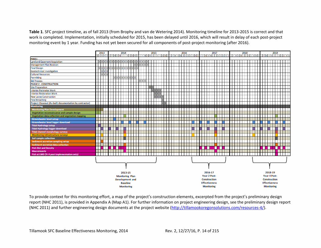
Project timeline and design overview
The original timeline for the SFC project construction and monitoring activities, as conceived in fall 2013, is shown in Table 1. The timing of 2013-2015 monitoring is accurate in Table 1, but additional activities have been added since 2013 that are not shown in the timeline:
• In addition to the monitoring activities shown in Table 1, “blue” carbon monitoring was added in 2015, and an additional sediment accretion sampling event is planned for 2016. Analysis is currently underway for the “blue” carbon monitoring (see Appendix G). Results from “blue” carbon monitoring and 2016 sediment accretion monitoring will be provided in a report delivered to Tillamook County in December 2016.
• Project implementation (Phase 1) has since been delayed until 2016, so Year 2 and Year 4 post-construction effectiveness monitoring will also be delayed by one year.
A current project timeline can be obtained from Rachel Hagerty, Tillamook County.
Tillamook SFC Baseline Effectiveness Monitoring, 2014 Rev. 2, 12/27/16, P. 14 of 215
Table 1. SFC project timeline, as of fall 2013 (from Brophy and van de Wetering 2014). Monitoring timeline for 2013-2015 is correct and that work is completed. Implementation, initially scheduled for 2015, has been delayed until 2016, which will result in delay of each post-project monitoring event by 1 year. Funding has not yet been secured for all components of post-project monitoring (after 2016).
To provide context for this monitoring effort, a map of the project’s construction elements, excerpted from the project’s preliminary design report (NHC 2011), is provided in Appendix A (Map A1). For further information on project engineering design, see the preliminary design report (NHC 2011) and further engineering design documents at the project website (http://tillamookoregonsolutions.com/resources-4/).
Tillamook SFC Baseline Effectiveness Monitoring, 2014 Rev. 2, 12/27/16, P. 15 of 215
Methods overview
As described above, this report is organized by effectiveness monitoring objectives; methods are briefly described under each objective, and summarized in Appendix C, Table C1. To provide context, sampling locations and the general sample design for the study are described below. Monitoring methods were based on a conceptual model of site functions (Brophy and van de Wetering 2014) and were designed to determine the project’s effectiveness in meeting its goals. Monitoring was also designed to be comparable with other projects, and to meet regional and national standards for science-based effectiveness monitoring of tidal wetland restoration projects (Rice et al. 2005, Roegner et al. 2008, Thayer et al. 2005, Simenstad et al. 1991). Further information on methods is available from the SFC Monitoring Plan (Brophy and van de Wetering 2014) and from the authors.
Study sites
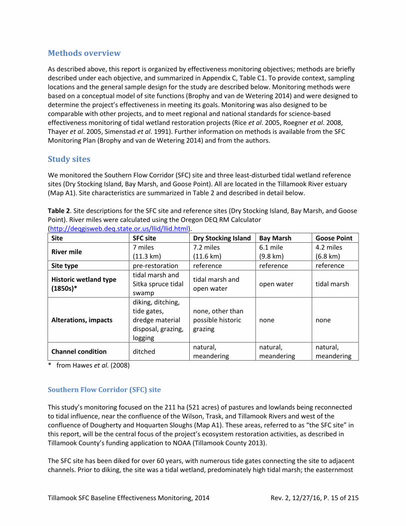
We monitored the Southern Flow Corridor (SFC) site and three least-disturbed tidal wetland reference sites (Dry Stocking Island, Bay Marsh, and Goose Point). All are located in the Tillamook River estuary (Map A1). Site characteristics are summarized in Table 2 and described in detail below. Table 2. Site descriptions for the SFC site and reference sites (Dry Stocking Island, Bay Marsh, and Goose Point). River miles were calculated using the Oregon DEQ RM Calculator (http://deqgisweb.deq.state.or.us/llid/llid.html).
Site SFC site Dry Stocking Island Bay Marsh Goose Point
River mile 7 miles (11.3 km)
7.2 miles (11.6 km)
6.1 mile (9.8 km)
4.2 miles (6.8 km)
Site type pre-restoration reference reference reference
Historic wetland type (1850s)*
tidal marsh and Sitka spruce tidal swamp
tidal marsh and open water
open water tidal marsh
Alterations, impacts
diking, ditching, tide gates, dredge material disposal, grazing, logging
none, other than possible historic grazing
none none
Channel condition ditched natural, meandering
natural, meandering
natural, meandering
* from Hawes et al. (2008)
Southern Flow Corridor (SFC) site This study’s monitoring focused on the 211 ha (521 acres) of pastures and lowlands being reconnected to tidal influence, near the confluence of the Wilson, Trask, and Tillamook Rivers and west of the confluence of Dougherty and Hoquarten Sloughs (Map A1). These areas, referred to as “the SFC site” in this report, will be the central focus of the project’s ecosystem restoration activities, as described in Tillamook County’s funding application to NOAA (Tillamook County 2013). The SFC site has been diked for over 60 years, with numerous tide gates connecting the site to adjacent channels. Prior to diking, the site was a tidal wetland, predominately high tidal marsh; the easternmost

Tillamook SFC Baseline Effectiveness Monitoring, 2014 Rev. 2, 12/27/16, P. 16 of 215
portions were tidal swamp (shrub/forested tidal wetland) dominated by Sitka spruce (Hawes et al. 2008). A limited area of forested wetland still occurs within the SFC site, primarily along the upper Blind Slough. However, based on discussion with project partners, forested areas were not monitored during this study, because forested wetland monitoring requires a disproportionately high time commitment compared to monitoring emergent wetlands. Another area omitted from sampling was the small area north of Blind Slough, adjacent to the Wilson River, and west of the Blind Slough tide gates. Although diked, this area experiences muted tidal flooding through small culverts without tide gates that drain into Blind Slough. This area was omitted from monitoring because it is so distinctly different from the rest of the SFC site, and monitoring results would therefore be atypical of the SFC site as a whole. The decision to focus monitoring on SFC’s diked emergent wetlands allowed robust and accurate evaluation of conditions within these wetlands, which constitute the vast majority of this project’s study area.
SFC site wetland sample zones Although elevation is relatively homogeneous across the SFC site, land use history and current land condition varies across the site. Therefore, sampling of the SFC site was stratified into zones reflecting this varied land use history, as described below and shown in Map A2.
North wetland zone
This zone consists of less-intensively-altered wetland area to the north of Blind Slough. This area was not ditched and appears not to have been tilled, at least in recent years. It has many meandering remnant tidal channels. Although this zone has been grazed in the past, grazing has not occurred for many years. This zone is abbreviated “North” in tables and figures.
Middle wetland zone
The Middle zone is abandoned pasture to the north of Goodspeed Road and south of Blind Slough. This zone has been actively managed as pasture in the past, and has several ditched drainages, but it also has many meandering remnant channels, in contrast to the South wetland zone. This zone is abbreviated “Middle” in tables and figures.
South (crop) wetland zone
The South (crop) zone consists of farmed land south of the centerline ditch, adjacent to the Trask River. This zone is heavily ditched and intensively managed, and has no meandering remnant channels. This zone is abbreviated “South crop” in tables and figures.
South (no-crop) wetland zone
This is a non-cropped area south of the centerline ditch and west of the South (cropped) wetland zone. Although this zone has been intensively managed in the relatively recent past (evidenced by ditched drainages and a lack of meandering remnant channels), it is currently neither grazed nor cropped. This zone is abbreviated “South no crop” in tables and figures.
Nolan Slough (crop) wetland zone
Nolan Slough (crop) is an intensively managed tilled land north of the Nolan Slough channel. As in the South zone, this area has been heavily ditched to facilitate cropping. This zone is abbreviated “Nolan crop” in tables and figures.
Tillamook SFC Baseline Effectiveness Monitoring, 2014 Rev. 2, 12/27/16, P. 17 of 215
Nolan Slough (grazed) wetland zone
Nolan Slough (grazed) is an active pasture surrounding Nolan Slough. The level of ditching in this zone is intermediate between the South wetland zone and the Middle wetland zone levels. This zone is abbreviated “Nolan grazed” in tables and figures.
Nolan Slough (ungrazed) wetland zone
Nolan Slough (ungrazed) is a wetland mitigation site south of Goodspeed Road. Since 2009, wetland mitigation activities in this zone have included excavation of meandering channels, and woody plantings. This zone is abbreviated “Nolan ungrazed” in tables and figures.
Fish monitoring zones
Blind Slough Mainstem
Blind Slough and its tributaries are the primary channel system for the North and Middle wetland zones. Prior to construction of the centerline ditch, the Blind Slough system probably carried the majority of daily tidal flows into the South wetland zone as well as the North and Middle zones.
Blind Slough Tributary
This tributary connects to Blind Slough just downstream of the Blind Slough Mainstem tide gates; it is also currently tide-gated. It is representative of the mid-sized tidal channels that predominate in the Middle wetland zone. The upper reach of this tributary is ditched, and is representative of the ditched channels found in the South wetland zone.
Nolan Slough
This channel system drains the eastern third of the main SFC project area. Historically, the middle and upper reaches of the Nolan Slough channel system were Sitka spruce tidal swamp (Hawes et al. 2008).
Reference sites Three least-disturbed reference sites provided examples of pre-disturbance conditions and goals for ecosystem restoration trajectory at the SFC site. Reference sites were selected to represent two different habitat classes: 1) high marsh, the historic habitat class that was likely prevalent across most of the SFC site prior to diking and conversion to agricultural use (Hawes et al. 2008); and 2) low marsh, the wetland class most likely to develop on the SFC site during the short term after project implementation, due to subsidence within the SFC site. In addition, reference site selection was also based on proximity and similar geomorphic setting to the SFC site. These similarities allow use of the “before-after-control-impact” (BACI) statistical framework, which optimizes interpretation of post-restoration changes at restoration sites (Stewart-Oaten et al. 1986, 1992).
Reference site wetland sample zones
Dry Stocking Island
This island is located at the confluence of the Trask and Tillamook rivers, and based on historic vegetation mapping (Hawes et al. 2008), it has expanded considerably since the mid- to late 1800s, due
Tillamook SFC Baseline Effectiveness Monitoring, 2014 Rev. 2, 12/27/16, P. 18 of 215
to high sediment loads carried by the estuary’s five major rivers (Phillip Williams and Associates 2002, Ewald and Brophy 2012). Despite historical actions to improve navigation in Hoquarten Slough (Coulton et al. 1996), channels and vegetation on the island appear to be undisturbed and in good condition (Ewald and Brophy 2012), supporting the selection of the island as a least-disturbed reference. Dry Stocking Island includes both low and high tidal marsh; we stratified sampling at this site within distinct low and high marsh areas defined using visual airphoto interpretation and DEMs (Map A4).
Bay Marsh
This site is an undiked low marsh located west of the SFC site, within the extensive marsh network that has accreted at the edge of Tillamook Bay since European settlement (Dicken 1961, Philip Williams and Associates 2002). During the immediate post-implementation period, tidal inundation regimes and other controlling factors at lower elevations at the SFC site are likely to be very similar to areas of similar elevation at Bay Marsh (Map A5).
Goose Point
The Goose Point wetlands are about 3 km (1.9 miles) north of the SFC site and were identified as least-disturbed tidal marsh in the Tillamook Tidal Wetland Prioritization (Ewald and Brophy 2012) and the Bay City Local Wetland Inventory (Wilson et al. 1997). This site contains mature, least-disturbed high marsh habitat, providing useful reference for pre-disturbance conditions at the SFC site as well as the site’s expected long-term post-implementation trajectory. However, salinities, tidal inundation patterns, and fluvial influence at Goose Point may differ from the SFC site and the Dry Stocking and Bay Marsh reference sites, due to Goose Point’s proximity to the mouth of Tillamook Bay and its landscape setting (bay fringe as opposed to river delta) (Map A6). Sampling at Goose Point focused on mature high marsh at elevations that are likely similar to the historic conditions at the SFC site (Maps A6 and A17).
Fish monitoring zones
Dry Stocking Island
This site’s channels provide a useful reference for fish use, habitat conditions, and macroinvertebrate communities in a least-disturbed tidal wetland immediately adjacent to the SFC site.
Wilson and Trask Rivers
Fish monitoring was conducted in the Wilson and Trask Rivers, which provide the “supply” of aquatic species for adjacent tidal wetlands and the SFC site.
General sample design
The sample design for this study had several components, summarized briefly below; for full details, see the SFC monitoring plan (Brophy and van de Wetering 2014). Sampling of aquatic biota (fish and macroinvertebrate) was designed to build understanding of how aquatic organisms used different habitats within the SFC site and reference sites, and was organized by sampling reaches (Maps A18-A19). Channel morphology monitoring focused on these aquatic biota sampling reaches, to allow calculation of fish access (Maps A15 and A17). Water level, salinity and water temperature were monitored at dual logger installations near these aquatic biota sampling reaches and in several other locations representing distinct hydrologic subunits of the study area (Maps A12 and A16-A17). Each installation included a water level logger and a combined conductivity/temperature logger. These
Tillamook SFC Baseline Effectiveness Monitoring, 2014 Rev. 2, 12/27/16, P. 19 of 215
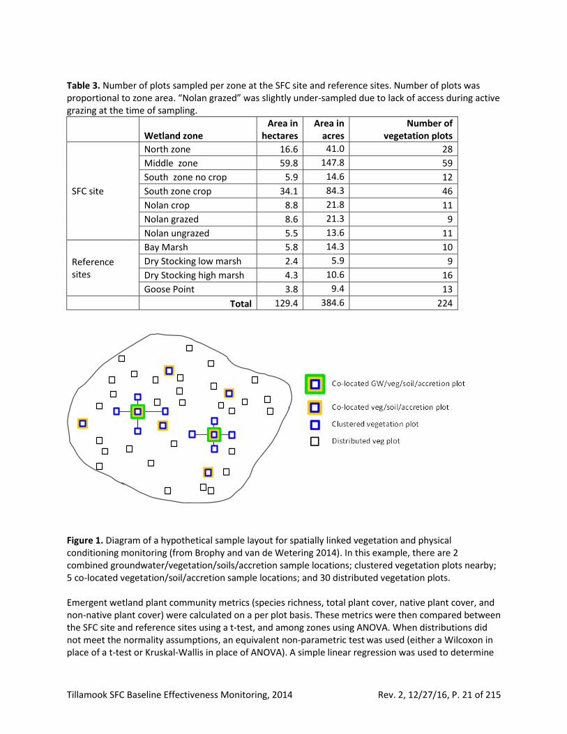
installations were placed in locations selected to represent major hydrologic zones within the study area. Finally, this study used a stratified random sample design for vegetation, soils, groundwater, and sediment accretion. This design maximized our ability to understand the relationships between these physical conditions and the associated plant communities. Strata for this stratified random design consisted of the wetland zones described above. Sample units within these zones (strata) consisted of vegetation plots (quadrats), soil cores, groundwater wells, and sediment accretion plots. A total of 224 vegetation plots were placed at random across all zones, using a plot randomization routine within ArcGIS. The number of plots per zone was proportional to zone area. Physical conditions monitoring was co-located with vegetation plots as follows (Figure 1):
• Groundwater sample stations (shallow observation wells) were placed in a randomly selected subgroup of 14 quadrats (3 in each wetland sample zone on the SFC project site, and 1 to 2 in high marsh at each reference site).
• Soil sampling and accretion/erosion sampling (feldspar marker horizon plots and sediment stakes) were co-located with the 14 groundwater sample stations, and also at an additional 24 randomly selected vegetation plots.
• Of the remaining 187 vegetation plots, 56 were clustered around the combined vegetation/physical drivers sample sites (Figure 1) to provide greater ability to interpret linkages between physical conditions and plant communities. These “clustered vegetation plots” were placed at N-S-E-W bearings and at random distances from the groundwater well.
• The remainder of the vegetation plots (168 quadrats) did not have associated physical conditions sampling (other than elevation, from which inundation regime could be calculated using nearby water level gauges).
• Elevation was determined for every vegetation quadrat using RTK-GPS.
METHODS AND RESULTS BY MONITORING OBJECTIVE
EM Objective 1: Vegetation
Quantify the development of vegetation communities within the SFC project site (including non-native and invasive species) and assess their degree of similarity to vegetation within reference wetlands.
Parameters: Plant species richness; percent cover (including non-native and invasive species); distribution and extent of plant communities
Emergent and tidal wetland plant communities Vegetation monitoring at the SFC site and nearby reference sites quantifies plant communities before the tidal reconnection event occurs, and tracks changes to plant communities after project implementation. As stated in Brophy and van de Wetering (2014), monitoring total plant cover, native species cover, non-native species cover, and species richness at the SFC site and nearby reference sites allows us to:
• Document changes in plant communities at the SFC site before and after project implementation, relative to reference sites;
• Document the degree to which native tidal wetland vegetation communities are re-established;
Tillamook SFC Baseline Effectiveness Monitoring, 2014 Rev. 2, 12/27/16, P. 20 of 215
• Provide information on relationships between vegetation development and hydrologic, topographic, and edaphic parameters such as wetland surface elevation, tidal hydrology/inundation regime, water and soil salinity fluctuations, soil characteristics, and groundwater level dynamics; and
• Document the presence and extent of invasive vegetation colonization, informing post-implementation adaptive management strategies, if needed.
Methods Baseline monitoring of emergent plant communities was conducted in August 2014 at the SFC site and nearby reference sites (Dry Stocking Island, Bay Marsh, and Goose Point). Sampling occurred in 224 randomized 1 m2 quadrats stratified by wetland sample zone at the SFC site and nearby reference sites. Numbers of samples per stratum were proportional to stratum area and randomized within stratum using computerized mapping (Geographic Information Systems) (Appendix D). A subset of plots were not randomized, but rather co-located with randomized groundwater wells, sediment accretion plots, and soil sample locations (Figure 1). By co-locating parameters, we could better interpret the linkages between plant community compositions and their physical drivers. At each vegetation plot, elevation was measured using an RTK-GPS receiver with a ten second occupation (Table 3). Visual estimates of species percent cover were made at each plot, following Bonham (1989). Scientific and common names of plants in this report are based on the Oregon Flora Project’s checklist (Cook et al. 2013). Percent cover represented the area within the plot that was covered, in vertical project, by the species in question. Percent cover estimates summed to 100% within a plot, including bare ground and other unvegetated surfaces. Vegetation was monitored mainly in emergent marsh/pasture, as that was the dominant habitat type through the SFC site. As described above, forested areas were not sampled, but when randomized plots occurred at the edge of forested areas, those were kept within the sampling. For these plots, percent cover of trees and shrubs was recorded in addition to emergent vegetation.
Tillamook SFC Baseline Effectiveness Monitoring, 2014 Rev. 2, 12/27/16, P. 21 of 215
Table 3. Number of plots sampled per zone at the SFC site and reference sites. Number of plots was proportional to zone area. “Nolan grazed” was slightly under-sampled due to lack of access during active grazing at the time of sampling.
Wetland zone Area in
hectares Area in
acres Number of
vegetation plots
SFC site
North zone 16.6 41.0 28
Middle zone 59.8 147.8 59
South zone no crop 5.9 14.6 12
South zone crop 34.1 84.3 46
Nolan crop 8.8 21.8 11
Nolan grazed 8.6 21.3 9
Nolan ungrazed 5.5 13.6 11
Reference sites
Bay Marsh 5.8 14.3 10
Dry Stocking low marsh 2.4 5.9 9
Dry Stocking high marsh 4.3 10.6 16
Goose Point 3.8 9.4 13
Total 129.4 384.6 224
Figure 1. Diagram of a hypothetical sample layout for spatially linked vegetation and physical conditioning monitoring (from Brophy and van de Wetering 2014). In this example, there are 2 combined groundwater/vegetation/soils/accretion sample locations; clustered vegetation plots nearby; 5 co-located vegetation/soil/accretion sample locations; and 30 distributed vegetation plots. Emergent wetland plant community metrics (species richness, total plant cover, native plant cover, and non-native plant cover) were calculated on a per plot basis. These metrics were then compared between the SFC site and reference sites using a t-test, and among zones using ANOVA. When distributions did not meet the normality assumptions, an equivalent non-parametric test was used (either a Wilcoxon in place of a t-test or Kruskal-Wallis in place of ANOVA). A simple linear regression was used to determine
Tillamook SFC Baseline Effectiveness Monitoring, 2014 Rev. 2, 12/27/16, P. 22 of 215
the relationship between elevation and species richness at the SFC site, and an exponential function was used for the reference sites, as it better fit the data. We ran a multi-response permutation procedure (999 permutations) and SIMPER analysis on plant community composition to determine if our grouping by zones were statistically significant in regards to plant species present, and to indicate which plant species were responsible for the differences between the SFC site and reference sites, as well as among zones. A multivariate technique, non-metric multidimensional scaling (NMDS), was used to summarize and visualize differences in plant community composition between the SFC site and reference sites. All analyses were completed in R (Version 3.1.1) using percent cover per plot as the dependent variable. Multivariate analyses were run using the R package vegan (Version 2.1.1). Differences in plant community metrics (species richness, total plant cover, native plant cover, and non-native plant cover) between the SFC site and reference sites, as well as between high marsh and low marsh habitats, were determined with a two-way ANOVA. Plots at elevations below locally-calculated MHHW (Figure 13) were categorized as low marsh, and plots at elevations higher than local MHHW (Table 4) were categorized as high marsh (Brophy et al. 2011, Janousek and Folger 2014). In the sections below, the term “dominant” was used for species that had the highest percent cover within the study transect. Species with more than 20% cover are commonly considered dominant, although species with less than 20% cover may be considered dominant when total cover is low (i.e., when bare ground is prevalent) (Tables 4-5). Table 4. Average elevations of vegetation plots at the SFC site and nearby reference marshes.
Site and wetland class
Average elevation in meters NAVD88,
Geoid 12A (standard error)
Average elevation in feet NAVD88,
Geoid 12A (standard error)
Dominant species or cover
SFC site 2.04 (0.02) 6.70 (0.06) reed canarygrass
Reference (low tidal marsh) 2.11 (0.04) 6.93 (0.25) Lyngbye’s sedge
Reference (high tidal marsh) 2.69 (0.03) 8.84 (0.10) tufted hairgrass
Table 5. Dominant plant species in sample zones at the SFC site and nearby reference marshes.
Zone Dominant species or cover
SFC site
North zone reed canarygrass
Middle zone reed canarygrass, slough sedge
South zone no crop reed canarygrass
South zone crop reed canarygrass
Nolan crop creeping bentgrass, meadow foxtail, tall fescue
Nolan grazed creeping bentgrass
Nolan ungrazed reed canarygrass, slough sedge
Reference sites
Bay Marsh low marsh creeping bentgrass, Lyngbye’s sedge
Dry Stocking Island low marsh Lyngbye’s sedge
Dry Stocking Island high marsh tufted hairgrass
Goose Point high marsh Pacific silverweed
Tillamook SFC Baseline Effectiveness Monitoring, 2014 Rev. 2, 12/27/16, P. 23 of 215
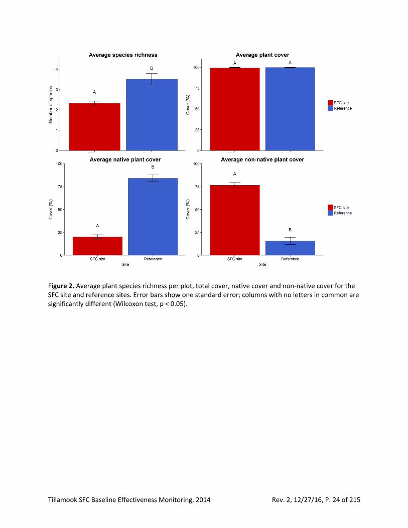
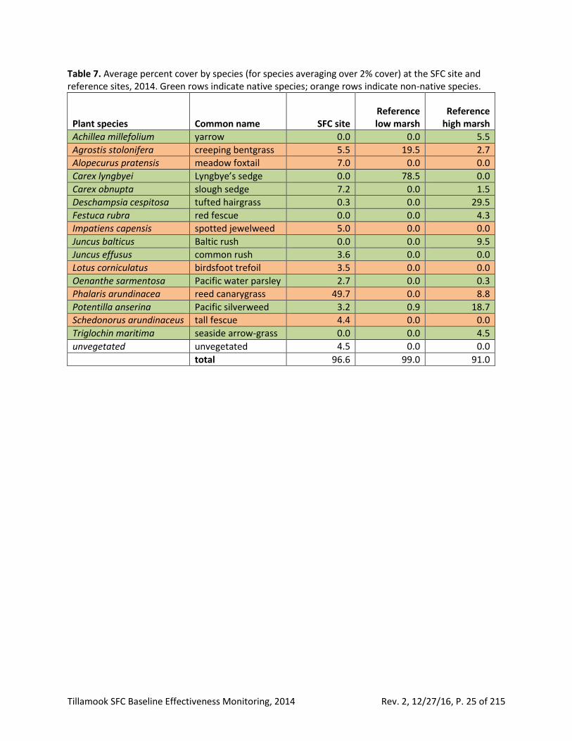
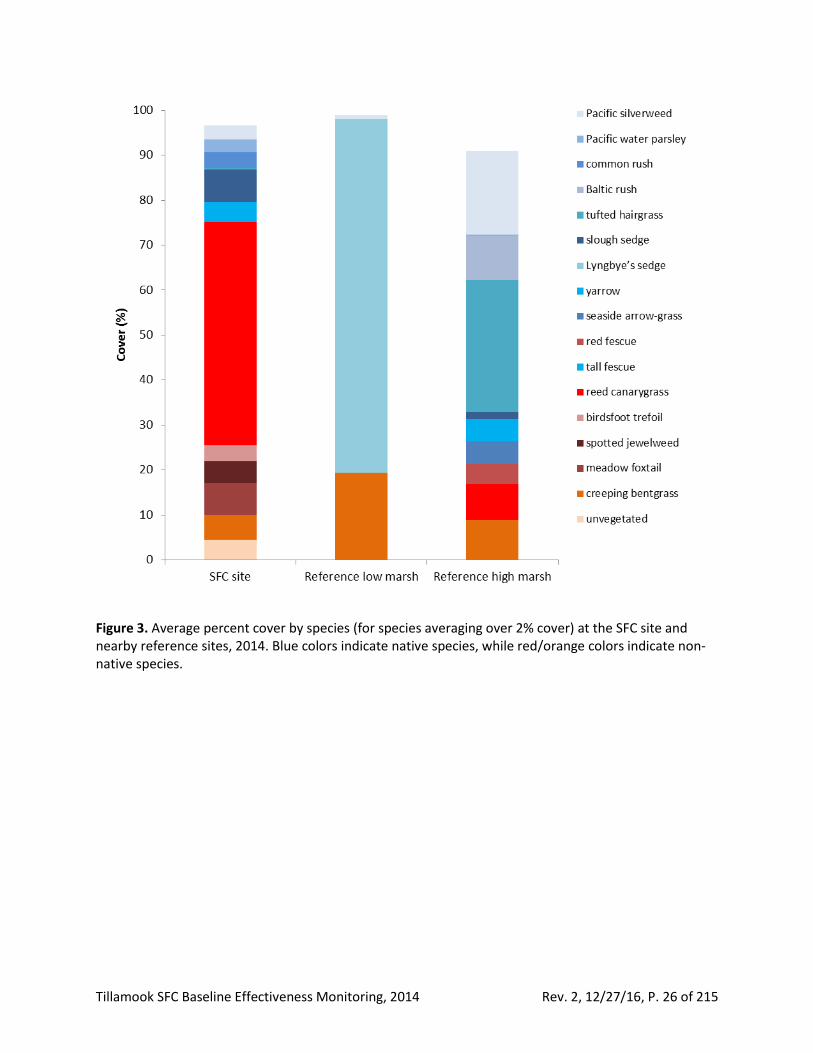
Results and discussion All derived plant community metrics except total plant cover differed significantly between the SFC site and reference sites. Species richness per plot and native species percent cover were significantly lower at the SFC site, and conversely, non-native species percent cover was significantly higher at the SFC site (Table 6, Figure 2). At the SFC site, average species richness per plot and native cover were 2.3 and 20%, respectively, while at the reference sites, they were 3.5 and 84%, respectively. Total cover was about 99% at the SFC site and reference sites. Note that species richness per plot does not reflect total species richness across plots. A total of 18 plant species averaged >2% cover across all plots at the SFC site (Table 7), and 13 species averaged >2% cover across all plots at the reference sites (Table 7). Many additional species were present at <2% cover (data available on request). A complete list of species found in sample plots is found in Table 12. The SFC site was dominated by the non-native invasive species reed canarygrass (Phalaris arundinacea), which averaged 50% cover across the site (Table 7, Figure 3). Native species were also dominant in some areas of the SFC site (Table 7, Figure 3). Native species, such as Lyngbye’s sedge (Carex lyngbyei) and tufted hairgrass (Deschampsia cespitosa), dominated the low and high marsh habitats of the reference sites (respectively). There was a significant relationship between species richness and elevation at the SFC site and at the reference sites (p < 0.0001 at both; Figure 4). However, this relationship was much less meaningful at the SFC site, with an R2 value of 0.07, indicating that elevation explains only 7% of species richness variability, versus 61% of variability at the reference site. Other researchers have observed strong correlations between species richness and elevation (e.g., Gough et al. 1994, Grace and Pugeske 1997, Kunza and Pennings 2008, Janousek and Folger 2014). Table 6. Average, standard error, and results of statistical tests for differences in plant community metrics, SFC site versus reference sites, 2014. Bold text indicates significant differences (p < 0.05).
Average (standard error) p-value
Species richness per plot
SFC site 2.3 (0.1) < 0.0001
reference sites 3.5 (0.3)
Total plant cover (%) SFC site 99.5 (0.2)
0.84 reference sites 99.8 (0.1)
Native cover (%) SFC site 20.0 (2.4)
< 0.0001 reference sites 84.2 (3.9)
Non-native cover (%) SFC site 76.6 (2.5)
< 0.0001 reference sites 15.6 (3.9)
Tillamook SFC Baseline Effectiveness Monitoring, 2014 Rev. 2, 12/27/16, P. 24 of 215
Figure 2. Average plant species richness per plot, total cover, native cover and non-native cover for the SFC site and reference sites. Error bars show one standard error; columns with no letters in common are significantly different (Wilcoxon test, p < 0.05).
Tillamook SFC Baseline Effectiveness Monitoring, 2014 Rev. 2, 12/27/16, P. 25 of 215
Table 7. Average percent cover by species (for species averaging over 2% cover) at the SFC site and reference sites, 2014. Green rows indicate native species; orange rows indicate non-native species.
Plant species Common name SFC site Reference low marsh
Reference high marsh
Achillea millefolium yarrow 0.0 0.0 5.5
Agrostis stolonifera creeping bentgrass 5.5 19.5 2.7
Alopecurus pratensis meadow foxtail 7.0 0.0 0.0
Carex lyngbyei Lyngbye’s sedge 0.0 78.5 0.0
Carex obnupta slough sedge 7.2 0.0 1.5
Deschampsia cespitosa tufted hairgrass 0.3 0.0 29.5
Festuca rubra red fescue 0.0 0.0 4.3
Impatiens capensis spotted jewelweed 5.0 0.0 0.0
Juncus balticus Baltic rush 0.0 0.0 9.5
Juncus effusus common rush 3.6 0.0 0.0
Lotus corniculatus birdsfoot trefoil 3.5 0.0 0.0
Oenanthe sarmentosa Pacific water parsley 2.7 0.0 0.3
Phalaris arundinacea reed canarygrass 49.7 0.0 8.8
Potentilla anserina Pacific silverweed 3.2 0.9 18.7
Schedonorus arundinaceus tall fescue 4.4 0.0 0.0
Triglochin maritima seaside arrow-grass 0.0 0.0 4.5
unvegetated unvegetated 4.5 0.0 0.0
total 96.6 99.0 91.0
Tillamook SFC Baseline Effectiveness Monitoring, 2014 Rev. 2, 12/27/16, P. 26 of 215
Figure 3. Average percent cover by species (for species averaging over 2% cover) at the SFC site and nearby reference sites, 2014. Blue colors indicate native species, while red/orange colors indicate non-native species.
Tillamook SFC Baseline Effectiveness Monitoring, 2014 Rev. 2, 12/27/16, P. 27 of 215
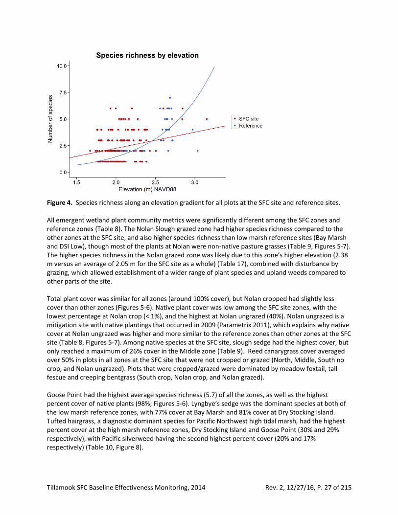
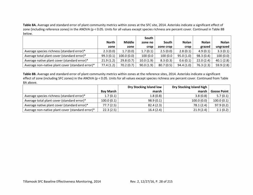
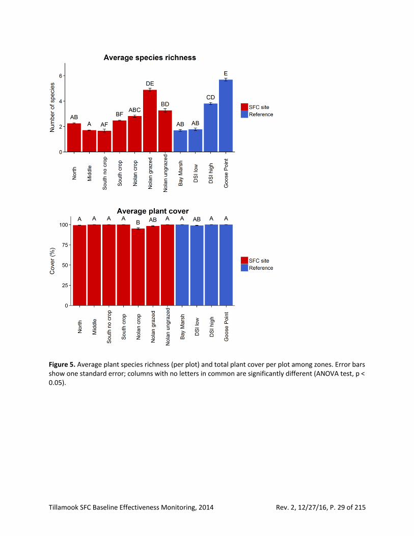
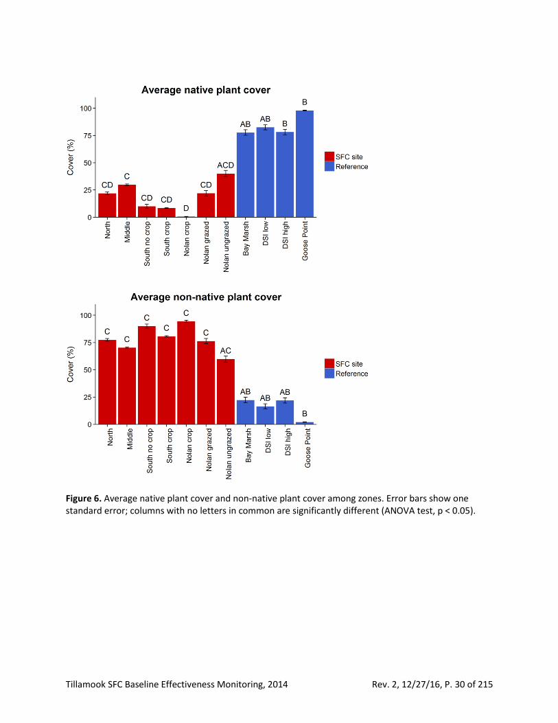
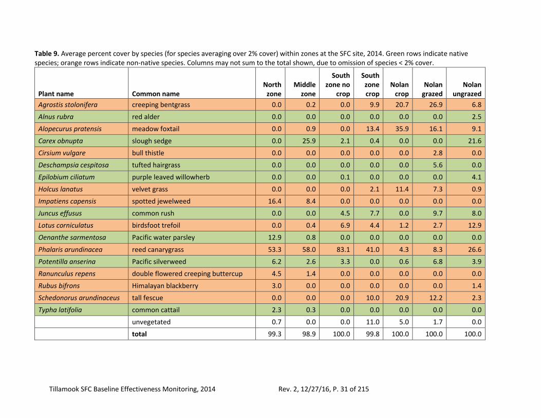
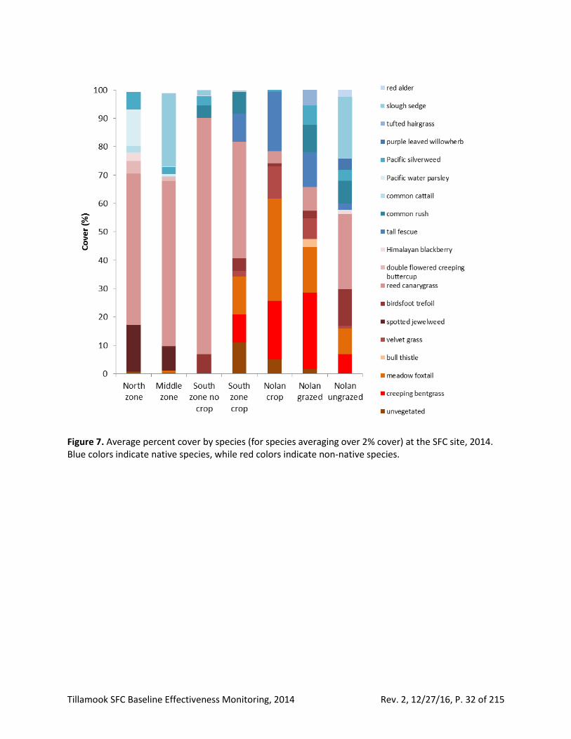
Figure 4. Species richness along an elevation gradient for all plots at the SFC site and reference sites. All emergent wetland plant community metrics were significantly different among the SFC zones and reference zones (Table 8). The Nolan Slough grazed zone had higher species richness compared to the other zones at the SFC site, and also higher species richness than low marsh reference sites (Bay Marsh and DSI Low), though most of the plants at Nolan were non-native pasture grasses (Table 9, Figures 5-7). The higher species richness in the Nolan grazed zone was likely due to this zone’s higher elevation (2.38 m versus an average of 2.05 m for the SFC site as a whole) (Table 17), combined with disturbance by grazing, which allowed establishment of a wider range of plant species and upland weeds compared to other parts of the site. Total plant cover was similar for all zones (around 100% cover), but Nolan cropped had slightly less cover than other zones (Figures 5-6). Native plant cover was low among the SFC site zones, with the lowest percentage at Nolan crop (< 1%), and the highest at Nolan ungrazed (40%). Nolan ungrazed is a mitigation site with native plantings that occurred in 2009 (Parametrix 2011), which explains why native cover at Nolan ungrazed was higher and more similar to the reference zones than other zones at the SFC site (Table 8, Figures 5-7). Among native species at the SFC site, slough sedge had the highest cover, but only reached a maximum of 26% cover in the Middle zone (Table 9). Reed canarygrass cover averaged over 50% in plots in all zones at the SFC site that were not cropped or grazed (North, Middle, South no crop, and Nolan ungrazed). Plots that were cropped/grazed were dominated by meadow foxtail, tall fescue and creeping bentgrass (South crop, Nolan crop, and Nolan grazed). Goose Point had the highest average species richness (5.7) of all the zones, as well as the highest percent cover of native plants (98%; Figures 5-6). Lyngbye’s sedge was the dominant species at both of the low marsh reference zones, with 77% cover at Bay Marsh and 81% cover at Dry Stocking Island. Tufted hairgrass, a diagnostic dominant species for Pacific Northwest high tidal marsh, had the highest percent cover at the high marsh reference zones, Dry Stocking Island and Goose Point (30% and 29% respectively), with Pacific silverweed having the second highest percent cover (20% and 17% respectively) (Table 10, Figure 8).
Tillamook SFC Baseline Effectiveness Monitoring, 2014 Rev. 2, 12/27/16, P. 28 of 215
Table 8A. Average and standard error of plant community metrics within zones at the SFC site, 2014. Asterisks indicate a significant effect of zone (including reference zones) in the ANOVA (p < 0.05. Units for all values except species richness are percent cover. Continued in Table 8B below.
North
zone Middle
zone
South zone no
crop South
zone crop Nolan
crop Nolan
grazed Nolan
ungrazed
Average species richness (standard error)* 2.3 (0.0) 1.7 (0.0) 1.7 (0.1) 2.5 (0.0) 2.8 (0.1) 4.9 (0.1) 3.3 (0.1)
Average total plant cover (standard error)* 99.3 (0.1) 100.0 (0.0) 100 (0.0 100 (0.0 95.0 (1.0) 98.3 (0.4) 100 (0.0)
Average native plant cover (standard error)* 21.9 (1.2) 29.8 (0.7) 10.0 (1.9) 8.3 (0.3) 0.6 (0.1) 22.0 (2.4) 40.1 (2.8)
Average non-native plant cover (standard error)* 77.4 (1.2) 70.2 (0.7) 90.0 (1.9) 80.7 (0.5) 94.4 (1.0) 76.3 (2.3) 59.9 (2.8)
Table 8B. Average and standard error of plant community metrics within zones at the reference sites, 2014. Asterisks indicate a significant effect of zone (including SFC zones) in the ANOVA (p < 0.05. Units for all values except species richness are percent cover. Continued from Table 8A above.
Bay Marsh Dry Stocking Island low
marsh Dry Stocking Island high
marsh Goose Point
Average species richness (standard error)* 1.7 (0.1) 1.8 (0.8) 3.8 (0.8) 5.7 (0.1)
Average total plant cover (standard error)* 100.0 (0.1) 98.9 (0.1) 100.0 (0.0) 100.0 (0.1)
Average native plant cover (standard error)* 77.7 (2.5) 82.4 (2.3) 78.1 (2.4) 97.9 (0.2)
Average non-native plant cover (standard error)* 22.3 (2.5) 16.4 (2.4) 21.9 (2.4) 2.1 (0.2)
Tillamook SFC Baseline Effectiveness Monitoring, 2014 Rev. 2, 12/27/16, P. 29 of 215
Figure 5. Average plant species richness (per plot) and total plant cover per plot among zones. Error bars show one standard error; columns with no letters in common are significantly different (ANOVA test, p < 0.05).
Tillamook SFC Baseline Effectiveness Monitoring, 2014 Rev. 2, 12/27/16, P. 30 of 215
Figure 6. Average native plant cover and non-native plant cover among zones. Error bars show one standard error; columns with no letters in common are significantly different (ANOVA test, p < 0.05).
Tillamook SFC Baseline Effectiveness Monitoring, 2014 Rev. 2, 12/27/16, P. 31 of 215
Table 9. Average percent cover by species (for species averaging over 2% cover) within zones at the SFC site, 2014. Green rows indicate native species; orange rows indicate non-native species. Columns may not sum to the total shown, due to omission of species < 2% cover.
Plant name Common name North
zone Middle
zone
South zone no
crop
South zone crop
Nolan crop
Nolan grazed
Nolan ungrazed
Agrostis stolonifera creeping bentgrass 0.0 0.2 0.0 9.9 20.7 26.9 6.8
Alnus rubra red alder 0.0 0.0 0.0 0.0 0.0 0.0 2.5
Alopecurus pratensis meadow foxtail 0.0 0.9 0.0 13.4 35.9 16.1 9.1
Carex obnupta slough sedge 0.0 25.9 2.1 0.4 0.0 0.0 21.6
Cirsium vulgare bull thistle 0.0 0.0 0.0 0.0 0.0 2.8 0.0
Deschampsia cespitosa tufted hairgrass 0.0 0.0 0.0 0.0 0.0 5.6 0.0
Epilobium ciliatum purple leaved willowherb 0.0 0.0 0.1 0.0 0.0 0.0 4.1
Holcus lanatus velvet grass 0.0 0.0 0.0 2.1 11.4 7.3 0.9
Impatiens capensis spotted jewelweed 16.4 8.4 0.0 0.0 0.0 0.0 0.0
Juncus effusus common rush 0.0 0.0 4.5 7.7 0.0 9.7 8.0
Lotus corniculatus birdsfoot trefoil 0.0 0.4 6.9 4.4 1.2 2.7 12.9
Oenanthe sarmentosa Pacific water parsley 12.9 0.8 0.0 0.0 0.0 0.0 0.0
Phalaris arundinacea reed canarygrass 53.3 58.0 83.1 41.0 4.3 8.3 26.6
Potentilla anserina Pacific silverweed 6.2 2.6 3.3 0.0 0.6 6.8 3.9
Ranunculus repens double flowered creeping buttercup 4.5 1.4 0.0 0.0 0.0 0.0 0.0
Rubus bifrons Himalayan blackberry 3.0 0.0 0.0 0.0 0.0 0.0 1.4
Schedonorus arundinaceus tall fescue 0.0 0.0 0.0 10.0 20.9 12.2 2.3
Typha latifolia common cattail 2.3 0.3 0.0 0.0 0.0 0.0 0.0
unvegetated 0.7 0.0 0.0 11.0 5.0 1.7 0.0
total 99.3 98.9 100.0 99.8 100.0 100.0 100.0
Tillamook SFC Baseline Effectiveness Monitoring, 2014 Rev. 2, 12/27/16, P. 32 of 215
Figure 7. Average percent cover by species (for species averaging over 2% cover) at the SFC site, 2014. Blue colors indicate native species, while red colors indicate non-native species.
Tillamook SFC Baseline Effectiveness Monitoring, 2014 Rev. 2, 12/27/16, P. 33 of 215
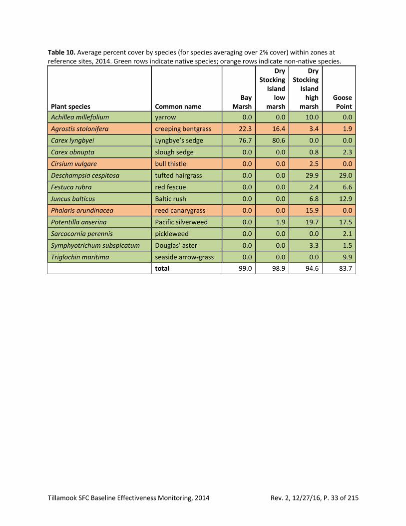
Table 10. Average percent cover by species (for species averaging over 2% cover) within zones at reference sites, 2014. Green rows indicate native species; orange rows indicate non-native species.
Plant species Common name Bay
Marsh
Dry Stocking
Island low
marsh
Dry Stocking
Island high
marsh Goose Point
Achillea millefolium yarrow 0.0 0.0 10.0 0.0
Agrostis stolonifera creeping bentgrass 22.3 16.4 3.4 1.9
Carex lyngbyei Lyngbye’s sedge 76.7 80.6 0.0 0.0
Carex obnupta slough sedge 0.0 0.0 0.8 2.3
Cirsium vulgare bull thistle 0.0 0.0 2.5 0.0
Deschampsia cespitosa tufted hairgrass 0.0 0.0 29.9 29.0
Festuca rubra red fescue 0.0 0.0 2.4 6.6
Juncus balticus Baltic rush 0.0 0.0 6.8 12.9
Phalaris arundinacea reed canarygrass 0.0 0.0 15.9 0.0
Potentilla anserina Pacific silverweed 0.0 1.9 19.7 17.5
Sarcocornia perennis pickleweed 0.0 0.0 0.0 2.1
Symphyotrichum subspicatum Douglas’ aster 0.0 0.0 3.3 1.5
Triglochin maritima seaside arrow-grass 0.0 0.0 0.0 9.9
total 99.0 98.9 94.6 83.7
Tillamook SFC Baseline Effectiveness Monitoring, 2014 Rev. 2, 12/27/16, P. 34 of 215
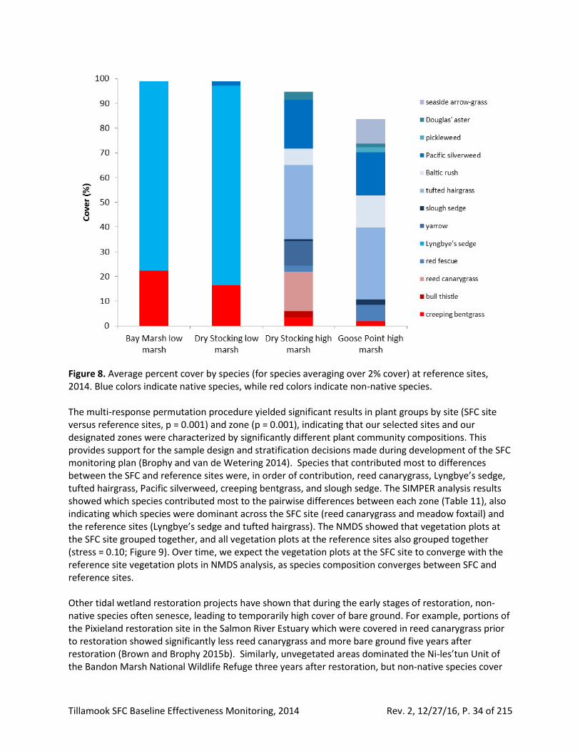
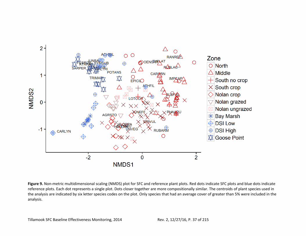
Figure 8. Average percent cover by species (for species averaging over 2% cover) at reference sites, 2014. Blue colors indicate native species, while red colors indicate non-native species. The multi-response permutation procedure yielded significant results in plant groups by site (SFC site versus reference sites, p = 0.001) and zone (p = 0.001), indicating that our selected sites and our designated zones were characterized by significantly different plant community compositions. This provides support for the sample design and stratification decisions made during development of the SFC monitoring plan (Brophy and van de Wetering 2014). Species that contributed most to differences between the SFC and reference sites were, in order of contribution, reed canarygrass, Lyngbye’s sedge, tufted hairgrass, Pacific silverweed, creeping bentgrass, and slough sedge. The SIMPER analysis results showed which species contributed most to the pairwise differences between each zone (Table 11), also indicating which species were dominant across the SFC site (reed canarygrass and meadow foxtail) and the reference sites (Lyngbye’s sedge and tufted hairgrass). The NMDS showed that vegetation plots at the SFC site grouped together, and all vegetation plots at the reference sites also grouped together (stress = 0.10; Figure 9). Over time, we expect the vegetation plots at the SFC site to converge with the reference site vegetation plots in NMDS analysis, as species composition converges between SFC and reference sites. Other tidal wetland restoration projects have shown that during the early stages of restoration, non-native species often senesce, leading to temporarily high cover of bare ground. For example, portions of the Pixieland restoration site in the Salmon River Estuary which were covered in reed canarygrass prior to restoration showed significantly less reed canarygrass and more bare ground five years after restoration (Brown and Brophy 2015b). Similarly, unvegetated areas dominated the Ni-les’tun Unit of the Bandon Marsh National Wildlife Refuge three years after restoration, but non-native species cover

Tillamook SFC Baseline Effectiveness Monitoring, 2014 Rev. 2, 12/27/16, P. 35 of 215
had dropped significantly (Brophy et al. 2014). This outcome is initially expected at the SFC site as well, but over several years, we expect native species to return to the site. Since the majority of the SFC site will be restored to low marsh (based on its average elevation 39 cm below MHHW), vegetation at the site is likely to gradually come to resemble the plant communities at Bay Marsh and Dry Stocking Island low marsh. Results for differences between low and high marsh habitats across the SFC site and reference sites did not add any further insight beyond the differences already presented above. Therefore, those results are presented in Appendix E. As described in the SFC Monitoring Plan (Brophy and van de Wetering 2014), our monitoring focused on emergent marsh. Only a few plots at the SFC site had woody species present, and none of the plots at the reference sites had woody species present. Due to this sparse data statistical analysis was not deemed appropriate, so only descriptive statistics are presented below. Seven species of trees and shrubs were found in the monitoring plots (Table 13). Of the seven species, five were native and two were non-native (Himalayan blackberry and cut leaved blackberry). The North and Middle zones had the majority of the woody species present. These zones have not been grazed in recent history; the increased woody growth in these zones is probably due to release from grazing pressure and discontinuation of pasture maintenance.
Tillamook SFC Baseline Effectiveness Monitoring, 2014 Rev. 2, 12/27/16, P. 36 of 215
Table 11. Results of a SIMPER analysis indicating the individual species that contributed most to differences between each zone. Six letter codes indicate species, while the arrow indicates which zone had the higher percentage of that species. Green indicates native species, orange indicates non-native species, SFC zones are in red and reference zones are in blue. “DSI” indicates Dry Stocking Island.
North Middle South no
crop South
crop Nolan
crop Nolan
grazed Nolan
ungrazed Bay
marsh DSI low
marsh DSI high
marsh Goose Point
North
Middle PHAARU
<
South no crop
PHAARU <
PHAARU <
South crop
PHAARU ^
PHAARU ^
PHAARU ^
Nolan crop
PHAARU ^
PHAARU ^
PHAARU ^
PHAARU ^
Nolan grazed
PHAARU ^
PHAARU ^
PHAARU ^
PHAARU ^
ALOPRA ^
Nolan ungrazed
PHAARU ^
PHAARU ^
PHAARU ^
PHAARU ^
ALOPRA ^
PHAARU <
Bay Marsh
CARLYN <
CARLYN <
PHAARU ^
CARLYN <
CARLYN <
CARLYN <
CARLYN <
DSI low marsh
CARLYN <
CARLYN <
PHAARU ^
CARLYN <
CARLYN <
CARLYN <
CARLYN <
CARLYN ^
DSI high marsh
PHAARU ^
PHAARU ^
PHAARU ^
PHAARU ^
ALOPRA ^
DESCES <
PHAARU ^
CARLYN <
CARLYN ^
Goose Point
PHAARU ^
PHAARU ^
PHAARU ^
PHAARU ^
ALOPRA ^
DESCES <
DESCES <
CARLYN ^
CARLYN ^
DESCES ^
Tillamook SFC Baseline Effectiveness Monitoring, 2014 Rev. 2, 12/27/16, P. 37 of 215
Figure 9. Non-metric multidimensional scaling (NMDS) plot for SFC and reference plant plots. Red dots indicate SFC plots and blue dots indicate reference plots. Each dot represents a single plot. Dots closer together are more compositionally similar. The centroids of plant species used in the analysis are indicated by six letter species codes on the plot. Only species that had an average cover of greater than 5% were included in the analysis.
Tillamook SFC Baseline Effectiveness Monitoring, 2014 Rev. 2, 12/27/16, P. 38 of 215
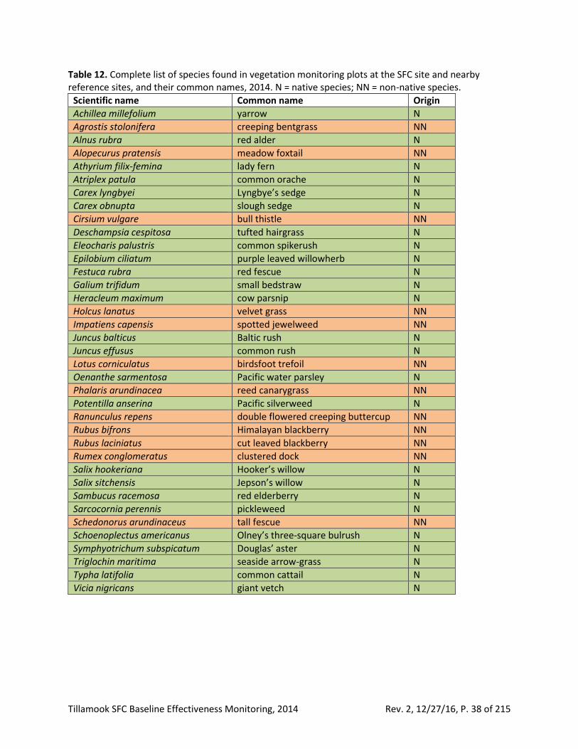
Table 12. Complete list of species found in vegetation monitoring plots at the SFC site and nearby reference sites, and their common names, 2014. N = native species; NN = non-native species.
Scientific name Common name Origin
Achillea millefolium yarrow N
Agrostis stolonifera creeping bentgrass NN
Alnus rubra red alder N
Alopecurus pratensis meadow foxtail NN
Athyrium filix-femina lady fern N
Atriplex patula common orache N
Carex lyngbyei Lyngbye’s sedge N
Carex obnupta slough sedge N
Cirsium vulgare bull thistle NN
Deschampsia cespitosa tufted hairgrass N
Eleocharis palustris common spikerush N
Epilobium ciliatum purple leaved willowherb N
Festuca rubra red fescue N
Galium trifidum small bedstraw N
Heracleum maximum cow parsnip N
Holcus lanatus velvet grass NN
Impatiens capensis spotted jewelweed NN
Juncus balticus Baltic rush N
Juncus effusus common rush N
Lotus corniculatus birdsfoot trefoil NN
Oenanthe sarmentosa Pacific water parsley N
Phalaris arundinacea reed canarygrass NN
Potentilla anserina Pacific silverweed N
Ranunculus repens double flowered creeping buttercup NN
Rubus bifrons Himalayan blackberry NN
Rubus laciniatus cut leaved blackberry NN
Rumex conglomeratus clustered dock NN
Salix hookeriana Hooker’s willow N
Salix sitchensis Jepson’s willow N
Sambucus racemosa red elderberry N
Sarcocornia perennis pickleweed N
Schedonorus arundinaceus tall fescue NN
Schoenoplectus americanus Olney’s three-square bulrush N
Symphyotrichum subspicatum Douglas’ aster N
Triglochin maritima seaside arrow-grass N
Typha latifolia common cattail N
Vicia nigricans giant vetch N
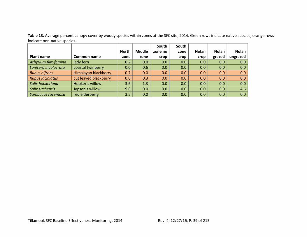
Tillamook SFC Baseline Effectiveness Monitoring, 2014 Rev. 2, 12/27/16, P. 39 of 215
Table 13. Average percent canopy cover by woody species within zones at the SFC site, 2014. Green rows indicate native species; orange rows indicate non-native species.
Plant name Common name North
zone Middle
zone
South zone no
crop
South zone crop
Nolan crop
Nolan grazed
Nolan ungrazed
Athyrium filix-femina lady fern 0.2 0.0 0.0 0.0 0.0 0.0 0.0
Lonicera involucrata coastal twinberry 0.0 0.6 0.0 0.0 0.0 0.0 0.0
Rubus bifrons Himalayan blackberry 0.7 0.0 0.0 0.0 0.0 0.0 0.0
Rubus laciniatus cut leaved blackberry 0.0 0.3 0.0 0.0 0.0 0.0 0.0
Salix hookeriana Hooker’s willow 3.6 1.3 0.0 0.0 0.0 0.0 0.0
Salix sitchensis Jepson’s willow 9.8 0.0 0.0 0.0 0.0 0.0 4.6
Sambucus racemosa red elderberry 3.5 0.0 0.0 0.0 0.0 0.0 0.0
Tillamook SFC Baseline Effectiveness Monitoring, 2014 Rev. 2, 12/27/16, P. 40 of 215
Plant community mapping
Methods We mapped wetland vegetation using aerial photography and field ground-truthing. We used the highest-resolution orthoimagery that was publicly available at the time of field work: 0.5 m resolution 2009 National Agricultural Image Program [NAIP] aerial photography provided by the State of Oregon at http://navigator.state.or.us/ArcGIS/services/Framework/Imagery_Mosaic2009/ImageServer. We printed a series of these aerial photographs at a scale of approximately 1:3000 with an accompanying UTM grid. These aerial printouts were carried to the field, where we traversed each project site on foot to correlate field vegetation with patterns in the aerial photographs. Map units (plant associations, described below) were delineated in the field on the aerial printouts. Digital vegetation maps were created in ArcGIS 10.3 by georeferencing the field maps and tracing the map unit boundaries into the GIS at a scale of 1:2000; the polygon size threshold was about 0.1 ha (0.25 ac). The vegetation map for each site was saved as a separate shapefile (with the final date inserted in each filename):
• SFC site: SFC_2015_vegmapping_20160228_LSB-FINAL.shp
• Dry Stocking Island reference site: DSI_2015_vegmapping_FINAL_[date].shp
• Bay Marsh reference site: BM_2015_vegmapping_FINAL_[date].shp
• Goose Point reference site: GP_2015_vegmapping_FINAL_[date].shp) These shapefiles are available from the Estuary Technical Group on request. Following the National Vegetation Classification Standard (The Nature Conservancy 1994), we used a two-level hierarchical vegetation classification scheme. Plant associations represented fine gradations of dominant species; these were finely divided to reflect small differences in community composition. Alliances, the coarser level, were described by a single major dominant species that characterized a larger area. This two-level classification allows flexibility in tracking future vegetation change. We also characterized plant communities as native-dominated or non-native-dominated, based on the alliance level classification. Native-species alliances such as Baltic rush and slough sedge were considered native-dominated, and non-native alliances such as reed canarygrass and tall fescue were considered non-native-dominated. The percent cover of native species versus non-native species varied within these alliances. As described in the SFC Effectiveness Monitoring Plan (Brophy and van de Wetering 2014), our monitoring focuses on the 211 ha (521 acres) of pastures and lowlands being reconnected to tidal influence, west of the confluence of Dougherty and Hoquarten Sloughs (Figure 3). These areas are the central focus of the NOAA restoration grant. As a result of this focus, our scope did not include monitoring or mapping of forested or scrub-shrub wetlands on the SFC site. However, we spent some field time characterizing the major canopy dominants (trees and shrubs) within the forested wetlands, and also used aerial photo interpretation to assist the final mapping (Appendix A, Map A8).
Results and discussion Based on plant community mapping results, plant communities at the SFC site were dominated by non-
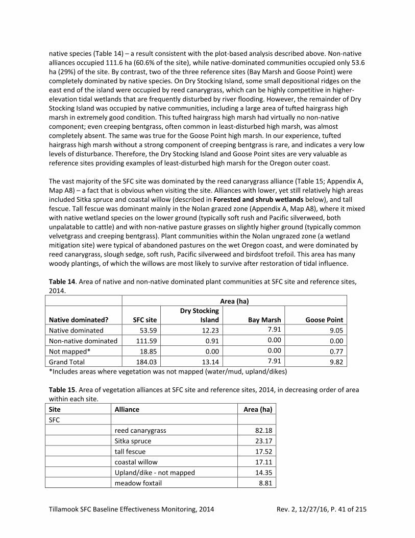
Tillamook SFC Baseline Effectiveness Monitoring, 2014 Rev. 2, 12/27/16, P. 41 of 215
native species (Table 14) – a result consistent with the plot-based analysis described above. Non-native alliances occupied 111.6 ha (60.6% of the site), while native-dominated communities occupied only 53.6 ha (29%) of the site. By contrast, two of the three reference sites (Bay Marsh and Goose Point) were completely dominated by native species. On Dry Stocking Island, some small depositional ridges on the east end of the island were occupied by reed canarygrass, which can be highly competitive in higher-elevation tidal wetlands that are frequently disturbed by river flooding. However, the remainder of Dry Stocking Island was occupied by native communities, including a large area of tufted hairgrass high marsh in extremely good condition. This tufted hairgrass high marsh had virtually no non-native component; even creeping bentgrass, often common in least-disturbed high marsh, was almost completely absent. The same was true for the Goose Point high marsh. In our experience, tufted hairgrass high marsh without a strong component of creeping bentgrass is rare, and indicates a very low levels of disturbance. Therefore, the Dry Stocking Island and Goose Point sites are very valuable as reference sites providing examples of least-disturbed high marsh for the Oregon outer coast. The vast majority of the SFC site was dominated by the reed canarygrass alliance (Table 15; Appendix A, Map A8) – a fact that is obvious when visiting the site. Alliances with lower, yet still relatively high areas included Sitka spruce and coastal willow (described in Forested and shrub wetlands below), and tall fescue. Tall fescue was dominant mainly in the Nolan grazed zone (Appendix A, Map A8), where it mixed with native wetland species on the lower ground (typically soft rush and Pacific silverweed, both unpalatable to cattle) and with non-native pasture grasses on slightly higher ground (typically common velvetgrass and creeping bentgrass). Plant communities within the Nolan ungrazed zone (a wetland mitigation site) were typical of abandoned pastures on the wet Oregon coast, and were dominated by reed canarygrass, slough sedge, soft rush, Pacific silverweed and birdsfoot trefoil. This area has many woody plantings, of which the willows are most likely to survive after restoration of tidal influence. Table 14. Area of native and non-native dominated plant communities at SFC site and reference sites, 2014.
Area (ha)
Native dominated? SFC site Dry Stocking
Island Bay Marsh Goose Point
Native dominated 53.59 12.23 7.91 9.05
Non-native dominated 111.59 0.91 0.00 0.00
Not mapped* 18.85 0.00 0.00 0.77
Grand Total 184.03 13.14 7.91 9.82
*Includes areas where vegetation was not mapped (water/mud, upland/dikes) Table 15. Area of vegetation alliances at SFC site and reference sites, 2014, in decreasing order of area within each site.
Site Alliance Area (ha)
SFC
reed canarygrass 82.18
Sitka spruce 23.17
tall fescue 17.52
coastal willow 17.11
Upland/dike - not mapped 14.35
meadow foxtail 8.81
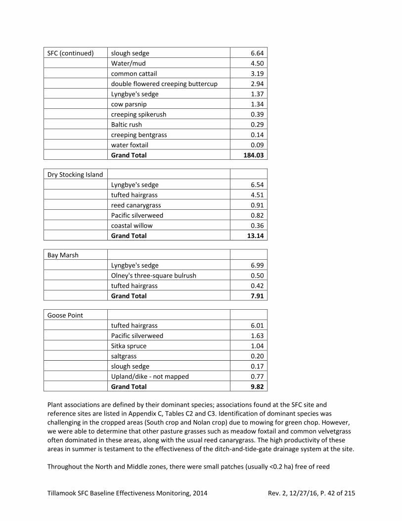
Tillamook SFC Baseline Effectiveness Monitoring, 2014 Rev. 2, 12/27/16, P. 42 of 215
SFC (continued) slough sedge 6.64
Water/mud 4.50
common cattail 3.19
double flowered creeping buttercup 2.94
Lyngbye's sedge 1.37
cow parsnip 1.34
creeping spikerush 0.39
Baltic rush 0.29
creeping bentgrass 0.14
water foxtail 0.09
Grand Total 184.03
Dry Stocking Island
Lyngbye's sedge 6.54
tufted hairgrass 4.51
reed canarygrass 0.91
Pacific silverweed 0.82
coastal willow 0.36
Grand Total 13.14
Bay Marsh
Lyngbye's sedge 6.99
Olney's three-square bulrush 0.50
tufted hairgrass 0.42
Grand Total 7.91
Goose Point
tufted hairgrass 6.01
Pacific silverweed 1.63
Sitka spruce 1.04
saltgrass 0.20
slough sedge 0.17
Upland/dike - not mapped 0.77
Grand Total 9.82
Plant associations are defined by their dominant species; associations found at the SFC site and reference sites are listed in Appendix C, Tables C2 and C3. Identification of dominant species was challenging in the cropped areas (South crop and Nolan crop) due to mowing for green chop. However, we were able to determine that other pasture grasses such as meadow foxtail and common velvetgrass often dominated in these areas, along with the usual reed canarygrass. The high productivity of these areas in summer is testament to the effectiveness of the ditch-and-tide-gate drainage system at the site. Throughout the North and Middle zones, there were small patches (usually <0.2 ha) free of reed

Tillamook SFC Baseline Effectiveness Monitoring, 2014 Rev. 2, 12/27/16, P. 43 of 215
canarygrass, dominated by double flowered creeping buttercup and Pacific silverweed. The reason for the absence of reed canarygrass from these areas is unknown; in winter, these patches are very heavily browsed by burrowing rodents (likely moles), taking on an almost “tilled” appearance from the rodents’ digging. The muted tidal wetland in the far northwest corner of the SFC site (northwest of the Blind Slough tide gates) was vegetated by a mix of primarily native wetland species, mainly slough sedge, soft rush, water parsley, and common cattail. Most of the dominant species at SFC are likely to die back after restoration of brackish tidal flows. Daily tidal flooding and increased summer salinities will most likely be beyond these species’ tolerances, although experience has shown that reed canarygrass and tall fescue may persist for many years in higher and fresher areas of tidal wetland restoration sites (Brophy 2017, Brophy et al. 2014, Brown and Brophy 2015b). Field studies at other sites in Oregon have shown a typical trajectory of short-term colonization by “fugitive” species and subsequent stabilization of vegetation (Cornu and Sadro 2002; Brown et al. 2015); but this process may take many years or even decades. Each stage of this trajectory may include a mix of native and non-native species.
SFC forested and shrub wetlands
Forested and shrub wetlands, generally dominated by Sitka spruce and coastal willow respectively, occupied about 40 ha (22%) of the SFC site. The shrub and herbaceous understory in these forested and shrub wetlands varied greatly depending on elevation, ranging from obligate wetlands species like slough sedge and skunk cabbage to transitional species like reed canarygrass and tall fescue. At lower elevations (most of the site), dominant trees included red alder as well as Sitka spruce, and dominant shrubs included black twinberry, Pacific crabapple, salmonberry, red elderberry, and coastal willow. Sitka willow and cascara were codominant in limited areas. Among these woody species, salinity tolerance varies widely. Although data are very sparse, our field studies have shown that among tidal swamp dominants, Sitka spruce, black twinberry, and Pacific crabapple are the most tolerant of brackish water; coastal willow and cascara are somewhat tolerant; and red alder, red elderberry, and salmonberry are relatively intolerant of brackish salinities (Brophy 2009, Brophy et al. 2011, 2014, 2015). Summer salinities are expected to be in the oligohaline to mesohaline range across SFC, although freshwater drainage from Hall Slough and the Wilson and Trask Rivers may allow fresher conditions to persist even in summer towards the east side of the site. Of course, in addition to the restored salinity regime, shrub and forested wetlands at the SFC site will also be strongly affected by the restored tidal inundation regime. The low elevations across the site will lead to daily tidal inundation even in summer, creating highly saturated or inundated conditions unsuitable for most of the current woody dominants. In the long term, coastal willow is probably the most likely to persist under these very wet post-restoration conditions. Although we did not map vegetation in uplands, we did note that in filled, disturbed areas (e.g., dredge material disposal areas, dikes, and roadways), the forest understory often includes weedy upland shrubs such as Himalayan blackberry, cutleaf blackberry, and Scots broom. These species are unlikely to return if these dikes and fill material are successfully removed and graded to the target tidal wetland elevation.
Tillamook SFC Baseline Effectiveness Monitoring, 2014 Rev. 2, 12/27/16, P. 44 of 215
SFC invasive species
We identified a number of invasive plant species at the SFC site, and several that could potentially be problematic. Fortunately, most of these invasives will be greatly reduced by restoration of brackish tidal flows, but some may persist in the fresher parts of the site. The guidance below is excerpted from our contributions to the SFC Baseline Documentation Report (Brown and Brophy 2015a) being prepared by Fritz Paulus: Current invasive species at SFC site:
• Reed canarygrass (Phalaris arundinacea): Not tolerant of high salinity, but may persist in low-brackish and freshwater tidal areas.
• Scotch broom (Cytisus scoparius): Upland species; should be greatly reduced by restoration but may persist on remaining dikes.
• Watermilfoil (Myriophyllum spp.): Widespread in channels. Not tolerant of high salinity, but may persist in low-brackish and freshwater tidal areas.
• Spotted jewelweed (Impatiens capensis): Widespread throughout the site. Not tolerant of salinity; should be greatly reduced by restoration of brackish tidal flows.
Potential invasive species at the SFC site:
• Yellow flag iris (Iris pseudacorus): Currently found on or near SFC; likely to invade fresh to brackish tidal wetlands. Monitoring is recommended, and control should be applied early if detected.
• Japanese knotweed (Fallopia japonica): Likely invader of riparian areas.
• Giant knotweed (Fallopia sachalinensis): Likely invader of riparian areas.
• Himalayan knotweed (Fallopia japonica): Likely invader of riparian areas.
• Common reed (Phragmites australis): May invade fresh or brackish tidal wetlands; monitoring is recommended, and control should be applied early if detected.
• Cordgrass (Spartina spp.): May invade tidal wetlands; monitoring is recommended, and control should be applied early if detected. Includes S. anglica, S. densiflora, S. patens, and S. alterniflora.
Reference sites
Tidal wetlands at the reference sites were vegetated by native species typical of high and low tidal marsh on Oregon’s outer coast. Low marsh at both the Dry Stocking Island and Bay Marsh sites was almost exclusively occupied by Lyngbye’s sedge, a highly productive perennial species that spreads by rhizomes and can form a very dense, tall canopy in summer, yet dies back to the soil surface in late fall leaving only its dense root system to overwinter. High marsh at Dry Stocking Island supported typical tidal marsh communities of tufted hairgrass, Baltic rush Pacific silverweed, with an extremely low proportion of non-natives. Even the non-native creeping bentgrass typically found intermingled with these species in least-disturbed high marsh in Oregon was absent from most of the eastern half of the island. Like Dry Stocking Island, the high marsh at Goose Point was in excellent condition, consisting almost entirely of native species, with little or none of the non-native creeping bentgrass often found in Oregon’s high marsh plant communities. The mix of native species in some parts of the Goose Point high
Tillamook SFC Baseline Effectiveness Monitoring, 2014 Rev. 2, 12/27/16, P. 45 of 215
marsh near the main tidal channel was unusual, however. In these areas, the typical high marsh species (tufted hairgrass, Baltic rush, and Pacific silverweed) were accompanied by a high component of common orache, a species that usually indicates either frequent disturbance by drift logs, or increasing salinity and vegetation change. Since drift logs were generally lacking on the surface of the Goose Point wetlands, it seems possible that vegetation is changing at this site. As noted in Ewald and Brophy (2012), the site does have a remnant dike (Ewald and Brophy 2012), but the dike appears to have long been breached; the site was never ditched; and its vegetation is almost entirely native, indicating a lack of past disturbance. However, it is possible that the remnant dike has had long-term effects on plant communities at the site. We recommend continuing to monitor Goose Point; it is a highly valuable reference site, since it is one of very few remaining least-disturbed high marsh sites left in the Tillamook Bay estuary.
EM Objective 2: Wetland physical conditions
Quantify changes in hydrologic, topographic, and edaphic parameters that support wetland functions and organisms using tidal wetland habitat. Parameters: Wetland surface elevation, tidal inundation regime, channel water salinity and temperature, groundwater regime, soil pH, soil salinity, soil % organic matter and carbon content, sediment accretion, channel morphology
Wetland surface elevation and water level Wetland surface elevation and water level are key ecological controlling factors in tidal wetlands (Thom et al. 2002), influencing plant community composition, groundwater level dynamics, sediment accretion rates, soil characteristics, and fish access. Monitoring baseline elevation and water level documents the current elevations and tidal restrictions prior to project implementation, providing data for post-project implementation comparisons and documenting the project’s effectiveness in re-establishing tidal influence to the SFC site. As stated in Brophy and van de Wetering (2014), results from monitoring of wetland surface elevations and water levels are used to:
• Document tidal restriction before project implementation;
• Document the degree to which SFC actions re-establish tidal influence;
• Provide data on controlling factors, to assist interpretation of other monitoring results such as plant communities and fish populations. Changes in water level are expected to relate closely to post-implementation trajectory for these and other parameters.
Methods Wetland surface elevation was calculated by averaging vegetation plot elevations by zone (Table 17). These measurements were collected at the ground surface using an RTK-GPS system with an occupation time of ten seconds. Tested vertical accuracy of each measurement was better than 6.5 cm at the 95% confidence level. Subsidence was calculated for each zone at the SFC site, as the difference between mean reference high marsh surface elevation and mean surface elevation within each zone. The elevation data had a non-normal distribution, so differences in marsh surface elevation and subsidence between the SFC site and reference sites were analyzed using a non-parametric Kruskal-Wallis rank sum test. Post-hoc non-parametric Wilcoxon rank sum tests with a Bonferroni adjustment were used to test differences among zones. All statistical analyses were performed in R (version 3.2.1).
Tillamook SFC Baseline Effectiveness Monitoring, 2014 Rev. 2, 12/27/16, P. 46 of 215
Water levels were measured using automated water level loggers (Onset HOBO© loggers, model U20-001-01), programmed to collect pressure data at 15 minute intervals. Water level monitoring began in late October of 2013 and continued until February 2015, covering two wet seasons and one dry season during the baseline period. Loggers were located along Blind Slough, Nolan Slough, and Trib 2 (a tributary within the SFC site) at the SFC site (Table 16, Map A12). The Blind Slough Upper logger was deployed from October 2013 through June 2014, but by June it was apparent that water levels would be below this logger all summer. Therefore, this location was abandoned and the Blind Slough Road location was substituted starting in July 2014. Reference loggers were placed at Goose Point, Bay Marsh, Dry Stocking Island, and the mouth of Blind Slough outside of the SFC site to provide data on nearby tidal water levels (Table 16, Maps A16-A17). For comparability, all loggers except Dry Stocking Island were installed so that their sensors were at approximately mean tide level, around 1.2 m NAVD88, based on NOAA’s Garibaldi tide gauge (MTL = 1.241 m NAVD88). The Dry Stocking Island sensor was placed as low as possible in the river channel, in order to capture the full tidal range. Its absolute elevation was relatively high for a full-range tide gauge (-0.34 m NAVD88), due to the relatively high river bed elevation. Despite this high elevation, this gauge successfully captured low tide water levels, because year-round river flows maintain an elevated low tide datum at this location (Figure 13). Water levels were tied to an orthometric reference frame (NAVD88) using a high-precision RTK GPS/GNSS system; loggers were checked for vertical movement at each maintenance interval by re-measuring the relationship between the sensor and a local benchmark with a laser level. These measurements had a standard deviation of 1.6 cm. There was no detectable persistent shift in logger elevation across the deployments. Raw logger data were converted from pressure values to water levels using HOBOWare Pro® software’s barometric compensation assistant, using local barometric pressure data collected onsite at 15 minute intervals throughout the monitoring period. Next, data were pruned to remove readings taken when the top of the logger body was submerged by less than 2 cm, or when the water temperature was below freezing (since loggers do not function well at temperatures <0° C). Tidal datums were calculated for logger installations at the reference sites in R (version 3.1.1) using the “Standard Method” and “Direct Method” as described in the NOAA Computational Techniques for Tidal Datums Handbook (NOAA 2003). The NOAA Garibaldi Tide Gauge (#9437540) in Tillamook Bay was the master station. Since NOAA does not provide a tie to an orthometric datum (such as NAVD88) for the Garibaldi gauge, we measured the elevations of NOAA’s nearby tidal benchmarks using high-precision RTK GPS/GNSS and tied the Garibaldi gauge elevation to NAVD88 (Geoid 12A). The Dry Stocking Island logger installation captured the full tidal range and was never exposed to air, allowing use of the “Standard Method” to calculate tidal datums: Mean Higher High Water (MHHW), Mean High Water (MHW), Mean Tide Level (MTL), Mean Low Water (MLW), and Mean Lower Low Water (MLLW). The “Standard Method” could not be applied to the Bay Marsh and Goose Point logger installations because they did not capture the full tidal range, so we used the “Direct Method” to calculate the MHHW and MHW tidal datum at these locations. Tidal datums were not calculated for logger installations within the SFC project because they are not currently subject to tidal influence. Tidal datums were not calculated for the Blind Slough Mouth logger because we expected its tidal inundation regime could be influenced by outflows from the SFC site; and because more suitable reference data were available from less-disturbed locations at Bay Marsh and Dry Stocking Island. We also conducted a tide-by-tide analysis to measure the difference in total water surface height and the time lag between tides at the reference site logger installations and the Garibaldi master station.
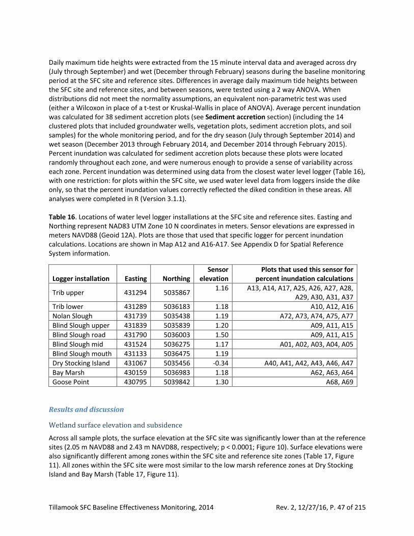
Tillamook SFC Baseline Effectiveness Monitoring, 2014 Rev. 2, 12/27/16, P. 47 of 215
Daily maximum tide heights were extracted from the 15 minute interval data and averaged across dry (July through September) and wet (December through February) seasons during the baseline monitoring period at the SFC site and reference sites. Differences in average daily maximum tide heights between the SFC site and reference sites, and between seasons, were tested using a 2 way ANOVA. When distributions did not meet the normality assumptions, an equivalent non-parametric test was used (either a Wilcoxon in place of a t-test or Kruskal-Wallis in place of ANOVA). Average percent inundation was calculated for 38 sediment accretion plots (see Sediment accretion section) (including the 14 clustered plots that included groundwater wells, vegetation plots, sediment accretion plots, and soil samples) for the whole monitoring period, and for the dry season (July through September 2014) and wet season (December 2013 through February 2014, and December 2014 through February 2015). Percent inundation was calculated for sediment accretion plots because these plots were located randomly throughout each zone, and were numerous enough to provide a sense of variability across each zone. Percent inundation was determined using data from the closest water level logger (Table 16), with one restriction: for plots within the SFC site, we used water level data from loggers inside the dike only, so that the percent inundation values correctly reflected the diked condition in these areas. All analyses were completed in R (Version 3.1.1). Table 16. Locations of water level logger installations at the SFC site and reference sites. Easting and Northing represent NAD83 UTM Zone 10 N coordinates in meters. Sensor elevations are expressed in meters NAVD88 (Geoid 12A). Plots are those that used that specific logger for percent inundation calculations. Locations are shown in Map A12 and A16-A17. See Appendix D for Spatial Reference System information.
Logger installation Easting Northing Sensor
elevation Plots that used this sensor for
percent inundation calculations
Trib upper 431294 5035867 1.16 A13, A14, A17, A25, A26, A27, A28,
A29, A30, A31, A37
Trib lower 431289 5036183 1.18 A10, A12, A16
Nolan Slough 431739 5035438 1.19 A72, A73, A74, A75, A77
Blind Slough upper 431839 5035839 1.20 A09, A11, A15
Blind Slough road 431790 5036003 1.50 A09, A11, A15
Blind Slough mid 431524 5036275 1.17 A01, A02, A03, A04, A05
Blind Slough mouth 431133 5036475 1.19
Dry Stocking Island 431067 5035456 -0.34 A40, A41, A42, A43, A46, A47
Bay Marsh 430159 5036983 1.18 A62, A63, A64
Goose Point 430795 5039842 1.30 A68, A69
Results and discussion
Wetland surface elevation and subsidence
Across all sample plots, the surface elevation at the SFC site was significantly lower than at the reference sites (2.05 m NAVD88 and 2.43 m NAVD88, respectively; p < 0.0001; Figure 10). Surface elevations were also significantly different among zones within the SFC site and reference site zones (Table 17, Figure 11). All zones within the SFC site were most similar to the low marsh reference zones at Dry Stocking Island and Bay Marsh (Table 17, Figure 11).
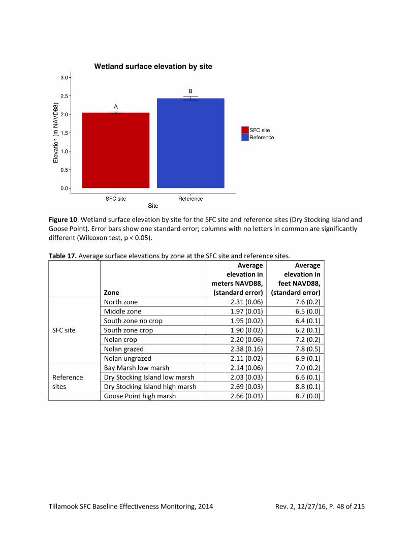
Tillamook SFC Baseline Effectiveness Monitoring, 2014 Rev. 2, 12/27/16, P. 48 of 215
Figure 10. Wetland surface elevation by site for the SFC site and reference sites (Dry Stocking Island and Goose Point). Error bars show one standard error; columns with no letters in common are significantly different (Wilcoxon test, p < 0.05). Table 17. Average surface elevations by zone at the SFC site and reference sites.
Zone
Average elevation in
meters NAVD88, (standard error)
Average elevation in
feet NAVD88, (standard error)
SFC site
North zone 2.31 (0.06) 7.6 (0.2)
Middle zone 1.97 (0.01) 6.5 (0.0)
South zone no crop 1.95 (0.02) 6.4 (0.1)
South zone crop 1.90 (0.02) 6.2 (0.1)
Nolan crop 2.20 (0.06) 7.2 (0.2)
Nolan grazed 2.38 (0.16) 7.8 (0.5)
Nolan ungrazed 2.11 (0.02) 6.9 (0.1)
Reference sites
Bay Marsh low marsh 2.14 (0.06) 7.0 (0.2)
Dry Stocking Island low marsh 2.03 (0.03) 6.6 (0.1)
Dry Stocking Island high marsh 2.69 (0.03) 8.8 (0.1)
Goose Point high marsh 2.66 (0.01) 8.7 (0.0)
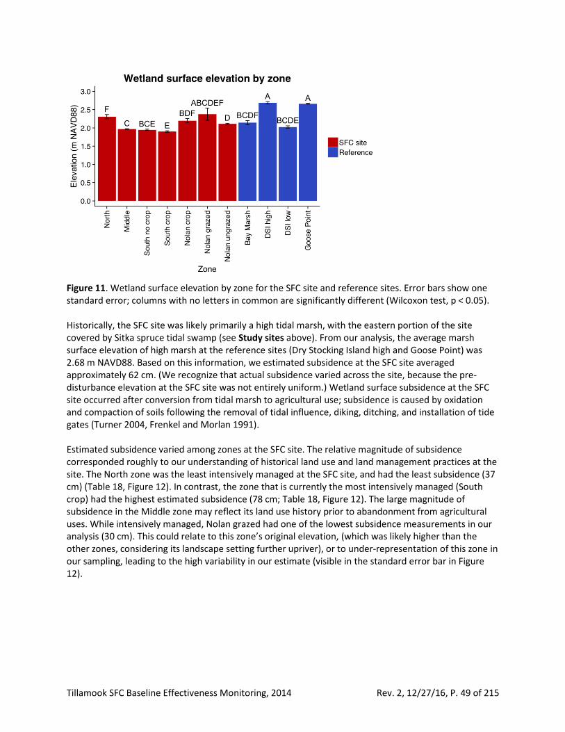
Tillamook SFC Baseline Effectiveness Monitoring, 2014 Rev. 2, 12/27/16, P. 49 of 215
Figure 11. Wetland surface elevation by zone for the SFC site and reference sites. Error bars show one standard error; columns with no letters in common are significantly different (Wilcoxon test, p < 0.05). Historically, the SFC site was likely primarily a high tidal marsh, with the eastern portion of the site covered by Sitka spruce tidal swamp (see Study sites above). From our analysis, the average marsh surface elevation of high marsh at the reference sites (Dry Stocking Island high and Goose Point) was 2.68 m NAVD88. Based on this information, we estimated subsidence at the SFC site averaged approximately 62 cm. (We recognize that actual subsidence varied across the site, because the pre-disturbance elevation at the SFC site was not entirely uniform.) Wetland surface subsidence at the SFC site occurred after conversion from tidal marsh to agricultural use; subsidence is caused by oxidation and compaction of soils following the removal of tidal influence, diking, ditching, and installation of tide gates (Turner 2004, Frenkel and Morlan 1991). Estimated subsidence varied among zones at the SFC site. The relative magnitude of subsidence corresponded roughly to our understanding of historical land use and land management practices at the site. The North zone was the least intensively managed at the SFC site, and had the least subsidence (37 cm) (Table 18, Figure 12). In contrast, the zone that is currently the most intensively managed (South crop) had the highest estimated subsidence (78 cm; Table 18, Figure 12). The large magnitude of subsidence in the Middle zone may reflect its land use history prior to abandonment from agricultural uses. While intensively managed, Nolan grazed had one of the lowest subsidence measurements in our analysis (30 cm). This could relate to this zone’s original elevation, (which was likely higher than the other zones, considering its landscape setting further upriver), or to under-representation of this zone in our sampling, leading to the high variability in our estimate (visible in the standard error bar in Figure 12).
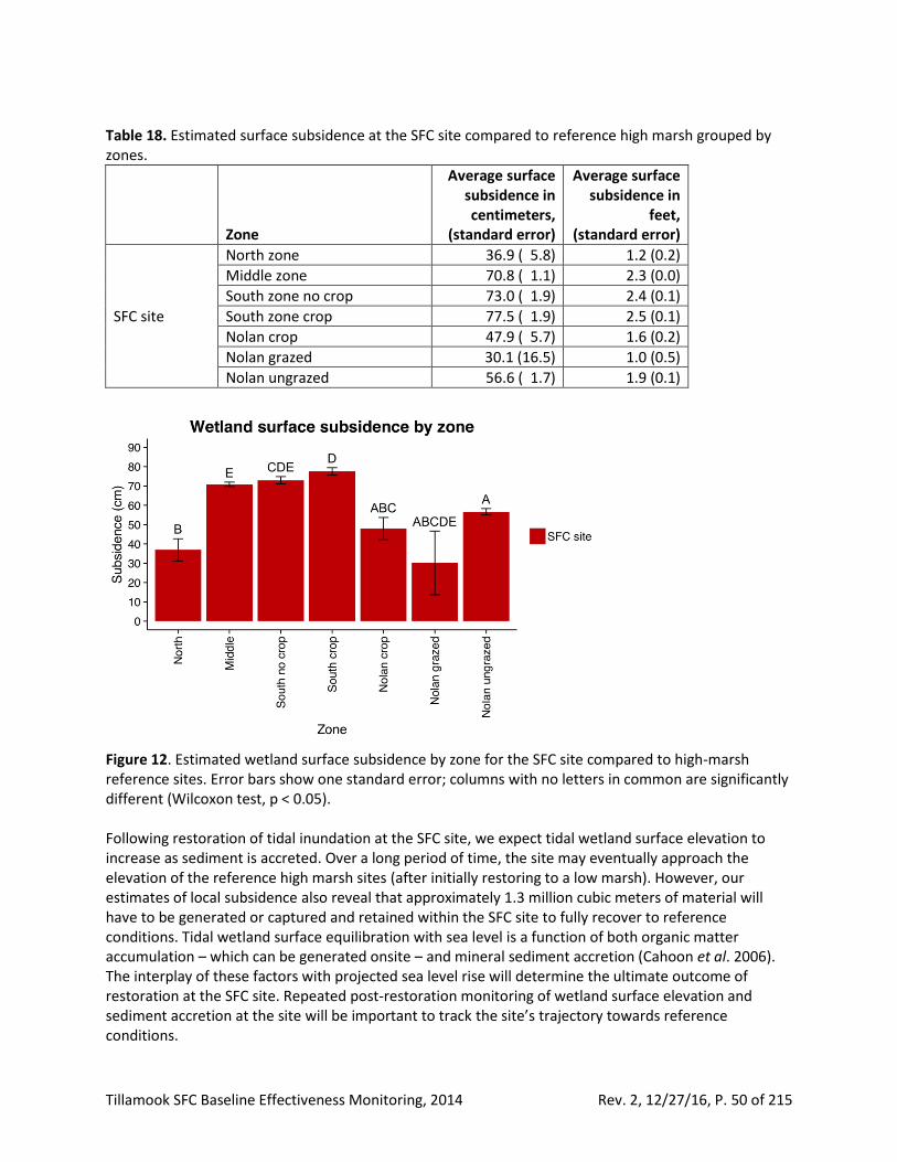
Tillamook SFC Baseline Effectiveness Monitoring, 2014 Rev. 2, 12/27/16, P. 50 of 215
Table 18. Estimated surface subsidence at the SFC site compared to reference high marsh grouped by zones.
Zone
Average surface subsidence in centimeters,
(standard error)
Average surface subsidence in
feet, (standard error)
SFC site
North zone 36.9 ( 5.8) 1.2 (0.2)
Middle zone 70.8 ( 1.1) 2.3 (0.0)
South zone no crop 73.0 ( 1.9) 2.4 (0.1)
South zone crop 77.5 ( 1.9) 2.5 (0.1)
Nolan crop 47.9 ( 5.7) 1.6 (0.2)
Nolan grazed 30.1 (16.5) 1.0 (0.5)
Nolan ungrazed 56.6 ( 1.7) 1.9 (0.1)
Figure 12. Estimated wetland surface subsidence by zone for the SFC site compared to high-marsh reference sites. Error bars show one standard error; columns with no letters in common are significantly different (Wilcoxon test, p < 0.05). Following restoration of tidal inundation at the SFC site, we expect tidal wetland surface elevation to increase as sediment is accreted. Over a long period of time, the site may eventually approach the elevation of the reference high marsh sites (after initially restoring to a low marsh). However, our estimates of local subsidence also reveal that approximately 1.3 million cubic meters of material will have to be generated or captured and retained within the SFC site to fully recover to reference conditions. Tidal wetland surface equilibration with sea level is a function of both organic matter accumulation – which can be generated onsite – and mineral sediment accretion (Cahoon et al. 2006). The interplay of these factors with projected sea level rise will determine the ultimate outcome of restoration at the SFC site. Repeated post-restoration monitoring of wetland surface elevation and sediment accretion at the site will be important to track the site’s trajectory towards reference conditions.
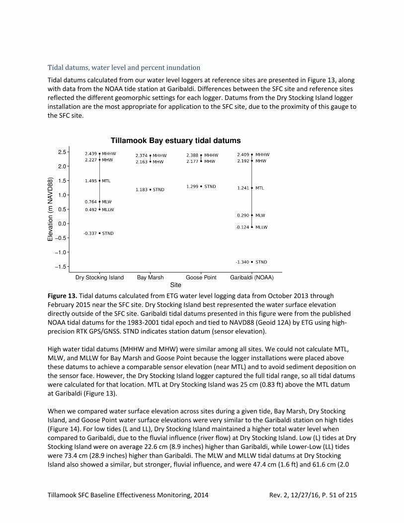
Tillamook SFC Baseline Effectiveness Monitoring, 2014 Rev. 2, 12/27/16, P. 51 of 215
Tidal datums, water level and percent inundation
Tidal datums calculated from our water level loggers at reference sites are presented in Figure 13, along with data from the NOAA tide station at Garibaldi. Differences between the SFC site and reference sites reflected the different geomorphic settings for each logger. Datums from the Dry Stocking Island logger installation are the most appropriate for application to the SFC site, due to the proximity of this gauge to the SFC site.
Figure 13. Tidal datums calculated from ETG water level logging data from October 2013 through February 2015 near the SFC site. Dry Stocking Island best represented the water surface elevation directly outside of the SFC site. Garibaldi tidal datums presented in this figure were from the published NOAA tidal datums for the 1983-2001 tidal epoch and tied to NAVD88 (Geoid 12A) by ETG using high-precision RTK GPS/GNSS. STND indicates station datum (sensor elevation). High water tidal datums (MHHW and MHW) were similar among all sites. We could not calculate MTL, MLW, and MLLW for Bay Marsh and Goose Point because the logger installations were placed above these datums to achieve a comparable sensor elevation (near MTL) and to avoid sediment deposition on the sensor face. However, the Dry Stocking Island logger captured the full tidal range, so all tidal datums were calculated for that location. MTL at Dry Stocking Island was 25 cm (0.83 ft) above the MTL datum at Garibaldi (Figure 13). When we compared water surface elevation across sites during a given tide, Bay Marsh, Dry Stocking Island, and Goose Point water surface elevations were very similar to the Garibaldi station on high tides (Figure 14). For low tides (L and LL), Dry Stocking Island maintained a higher total water level when compared to Garibaldi, due to the fluvial influence (river flow) at Dry Stocking Island. Low (L) tides at Dry Stocking Island were on average 22.6 cm (8.9 inches) higher than Garibaldi, while Lower-Low (LL) tides were 73.4 cm (28.9 inches) higher than Garibaldi. The MLW and MLLW tidal datums at Dry Stocking Island also showed a similar, but stronger, fluvial influence, and were 47.4 cm (1.6 ft) and 61.6 cm (2.0
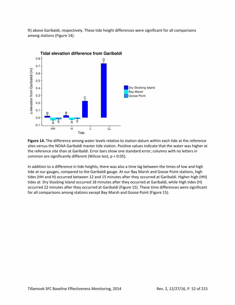
Tillamook SFC Baseline Effectiveness Monitoring, 2014 Rev. 2, 12/27/16, P. 52 of 215
ft) above Garibaldi, respectively. These tide height differences were significant for all comparisons among stations (Figure 14).
Figure 14. The difference among water levels relative to station datum within each tide at the reference sites versus the NOAA Garibaldi master tide station. Positive values indicate that the water was higher at the reference site than at Garibaldi. Error bars show one standard error; columns with no letters in common are significantly different (Wilcox test, p < 0.05). In addition to a difference in tide heights, there was also a time lag between the times of low and high tide at our gauges, compared to the Garibaldi gauge. At our Bay Marsh and Goose Point stations, high tides (HH and H) occurred between 12 and 15 minutes after they occurred at Garibaldi. Higher-high (HH) tides at Dry Stocking Island occurred 18 minutes after they occurred at Garibaldi, while High tides (H) occurred 22 minutes after they occurred at Garibaldi (Figure 15). These time differences were significant for all comparisons among stations except Bay Marsh and Goose Point (Figure 15).
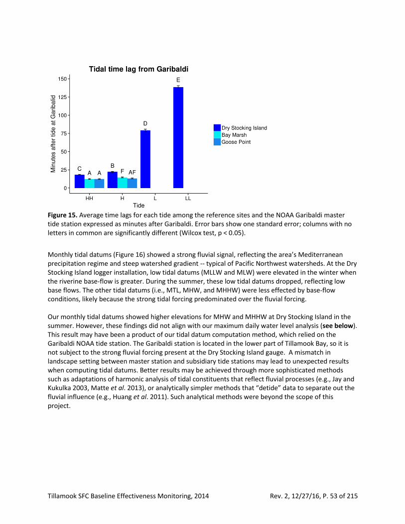
Tillamook SFC Baseline Effectiveness Monitoring, 2014 Rev. 2, 12/27/16, P. 53 of 215
Figure 15. Average time lags for each tide among the reference sites and the NOAA Garibaldi master tide station expressed as minutes after Garibaldi. Error bars show one standard error; columns with no letters in common are significantly different (Wilcox test, p < 0.05).
Monthly tidal datums (Figure 16) showed a strong fluvial signal, reflecting the area’s Mediterranean precipitation regime and steep watershed gradient -- typical of Pacific Northwest watersheds. At the Dry Stocking Island logger installation, low tidal datums (MLLW and MLW) were elevated in the winter when the riverine base-flow is greater. During the summer, these low tidal datums dropped, reflecting low base flows. The other tidal datums (i.e., MTL, MHW, and MHHW) were less effected by base-flow conditions, likely because the strong tidal forcing predominated over the fluvial forcing. Our monthly tidal datums showed higher elevations for MHW and MHHW at Dry Stocking Island in the summer. However, these findings did not align with our maximum daily water level analysis (see below). This result may have been a product of our tidal datum computation method, which relied on the Garibaldi NOAA tide station. The Garibaldi station is located in the lower part of Tillamook Bay, so it is not subject to the strong fluvial forcing present at the Dry Stocking Island gauge. A mismatch in landscape setting between master station and subsidiary tide stations may lead to unexpected results when computing tidal datums. Better results may be achieved through more sophisticated methods such as adaptations of harmonic analysis of tidal constituents that reflect fluvial processes (e.g., Jay and Kukulka 2003, Matte et al. 2013), or analytically simpler methods that “detide” data to separate out the fluvial influence (e.g., Huang et al. 2011). Such analytical methods were beyond the scope of this project.
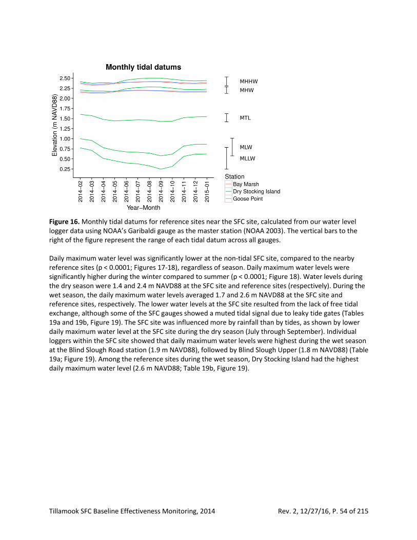
Tillamook SFC Baseline Effectiveness Monitoring, 2014 Rev. 2, 12/27/16, P. 54 of 215
Figure 16. Monthly tidal datums for reference sites near the SFC site, calculated from our water level logger data using NOAA’s Garibaldi gauge as the master station (NOAA 2003). The vertical bars to the right of the figure represent the range of each tidal datum across all gauges. Daily maximum water level was significantly lower at the non-tidal SFC site, compared to the nearby reference sites (p < 0.0001; Figures 17-18), regardless of season. Daily maximum water levels were significantly higher during the winter compared to summer (p < 0.0001; Figure 18). Water levels during the dry season were 1.4 and 2.4 m NAVD88 at the SFC site and reference sites (respectively). During the wet season, the daily maximum water levels averaged 1.7 and 2.6 m NAVD88 at the SFC site and reference sites, respectively. The lower water levels at the SFC site resulted from the lack of free tidal exchange, although some of the SFC gauges showed a muted tidal signal due to leaky tide gates (Tables 19a and 19b, Figure 19). The SFC site was influenced more by rainfall than by tides, as shown by lower daily maximum water level at the SFC site during the dry season (July through September). Individual loggers within the SFC site showed that daily maximum water levels were highest during the wet season at the Blind Slough Road station (1.9 m NAVD88), followed by Blind Slough Upper (1.8 m NAVD88) (Table 19a; Figure 19). Among the reference sites during the wet season, Dry Stocking Island had the highest daily maximum water level (2.6 m NAVD88; Table 19b, Figure 19).
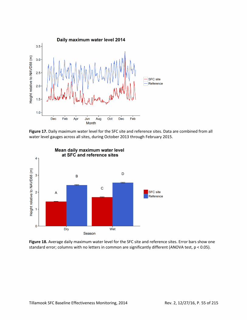
Tillamook SFC Baseline Effectiveness Monitoring, 2014 Rev. 2, 12/27/16, P. 55 of 215
Figure 17. Daily maximum water level for the SFC site and reference sites. Data are combined from all water level gauges across all sites, during October 2013 through February 2015.
Figure 18. Average daily maximum water level for the SFC site and reference sites. Error bars show one standard error; columns with no letters in common are significantly different (ANOVA test, p < 0.05).
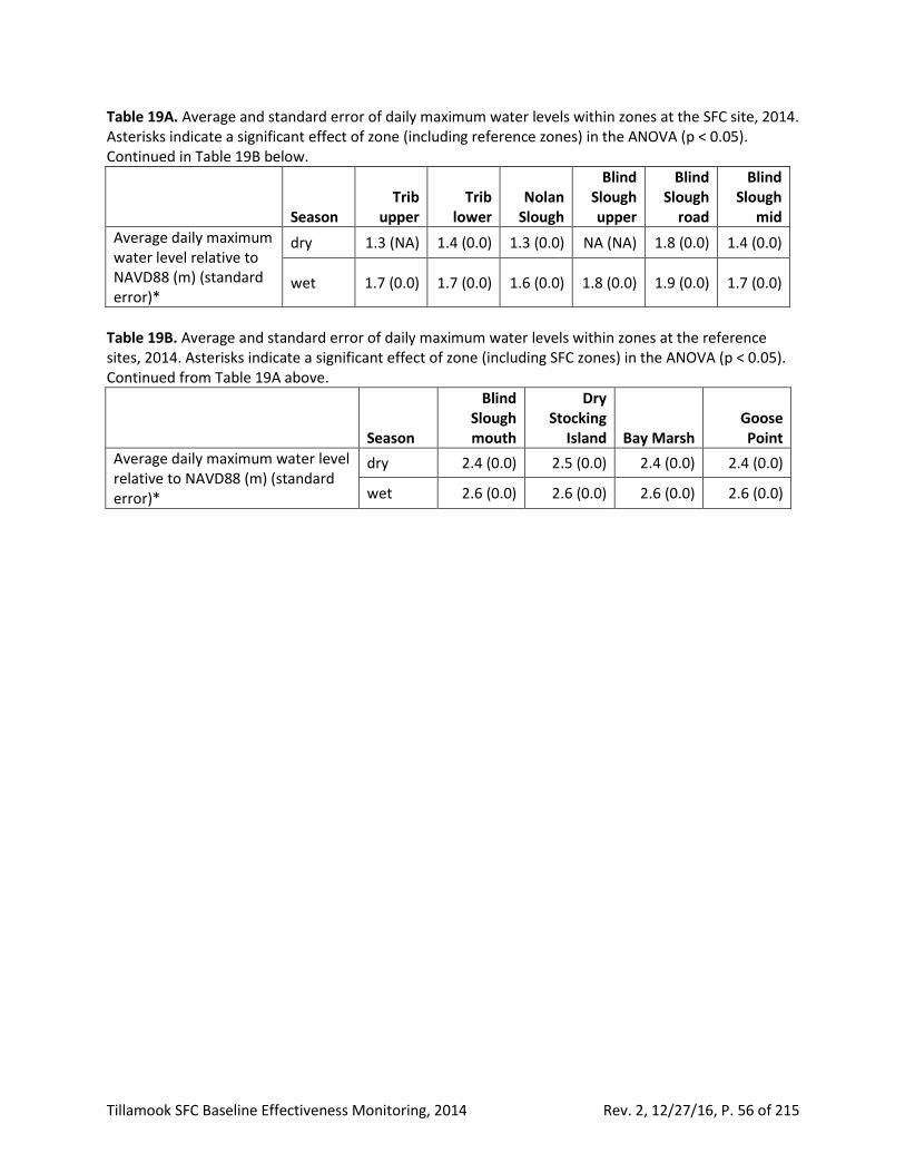
Tillamook SFC Baseline Effectiveness Monitoring, 2014 Rev. 2, 12/27/16, P. 56 of 215
Table 19A. Average and standard error of daily maximum water levels within zones at the SFC site, 2014. Asterisks indicate a significant effect of zone (including reference zones) in the ANOVA (p < 0.05). Continued in Table 19B below.
Season Trib
upper Trib
lower Nolan
Slough
Blind Slough upper
Blind Slough
road
Blind Slough
mid
Average daily maximum water level relative to NAVD88 (m) (standard error)*
dry 1.3 (NA) 1.4 (0.0) 1.3 (0.0) NA (NA) 1.8 (0.0) 1.4 (0.0)
wet 1.7 (0.0) 1.7 (0.0) 1.6 (0.0) 1.8 (0.0) 1.9 (0.0) 1.7 (0.0)
Table 19B. Average and standard error of daily maximum water levels within zones at the reference sites, 2014. Asterisks indicate a significant effect of zone (including SFC zones) in the ANOVA (p < 0.05). Continued from Table 19A above.
Season
Blind Slough mouth
Dry Stocking
Island Bay Marsh Goose Point
Average daily maximum water level relative to NAVD88 (m) (standard error)*
dry 2.4 (0.0) 2.5 (0.0) 2.4 (0.0) 2.4 (0.0)
wet 2.6 (0.0) 2.6 (0.0) 2.6 (0.0) 2.6 (0.0)
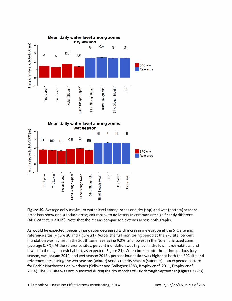
Tillamook SFC Baseline Effectiveness Monitoring, 2014 Rev. 2, 12/27/16, P. 57 of 215
Figure 19. Average daily maximum water level among zones and dry (top) and wet (bottom) seasons. Error bars show one standard error; columns with no letters in common are significantly different (ANOVA test, p < 0.05). Note that the means comparison extends across both graphs. As would be expected, percent inundation decreased with increasing elevation at the SFC site and reference sites (Figure 20 and Figure 21). Across the full monitoring period at the SFC site, percent inundation was highest in the South zone, averaging 9.2%; and lowest in the Nolan ungrazed zone (average 0.7%). At the reference sites, percent inundation was highest in the low marsh habitats, and lowest in the high marsh habitat, as expected (Figure 21). When broken into three time periods (dry season, wet season 2014, and wet season 2015), percent inundation was higher at both the SFC site and reference sites during the wet seasons (winter) versus the dry season (summer) -- an expected pattern for Pacific Northwest tidal wetlands (Seliskar and Gallagher 1983, Brophy et al. 2011, Brophy et al. 2014). The SFC site was not inundated during the dry months of July through September (Figures 22-23).
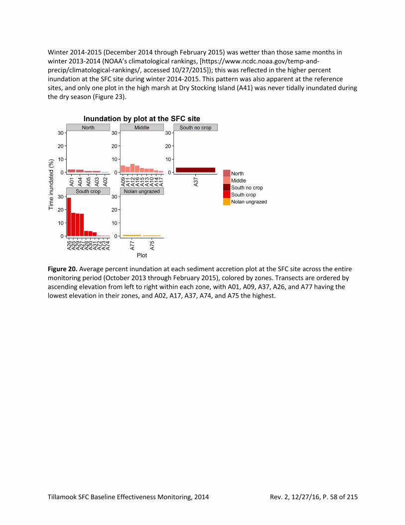
Tillamook SFC Baseline Effectiveness Monitoring, 2014 Rev. 2, 12/27/16, P. 58 of 215
Winter 2014-2015 (December 2014 through February 2015) was wetter than those same months in winter 2013-2014 (NOAA’s climatological rankings, [https://www.ncdc.noaa.gov/temp-and-precip/climatological-rankings/, accessed 10/27/2015]); this was reflected in the higher percent inundation at the SFC site during winter 2014-2015. This pattern was also apparent at the reference sites, and only one plot in the high marsh at Dry Stocking Island (A41) was never tidally inundated during the dry season (Figure 23).
Figure 20. Average percent inundation at each sediment accretion plot at the SFC site across the entire monitoring period (October 2013 through February 2015), colored by zones. Transects are ordered by ascending elevation from left to right within each zone, with A01, A09, A37, A26, and A77 having the lowest elevation in their zones, and A02, A17, A37, A74, and A75 the highest.
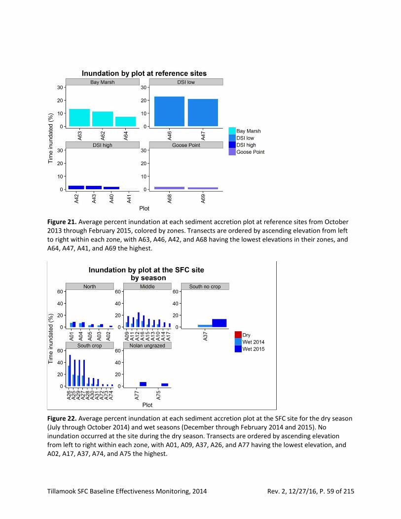
Tillamook SFC Baseline Effectiveness Monitoring, 2014 Rev. 2, 12/27/16, P. 59 of 215
Figure 21. Average percent inundation at each sediment accretion plot at reference sites from October 2013 through February 2015, colored by zones. Transects are ordered by ascending elevation from left to right within each zone, with A63, A46, A42, and A68 having the lowest elevations in their zones, and A64, A47, A41, and A69 the highest.
Figure 22. Average percent inundation at each sediment accretion plot at the SFC site for the dry season (July through October 2014) and wet seasons (December through February 2014 and 2015). No inundation occurred at the site during the dry season. Transects are ordered by ascending elevation from left to right within each zone, with A01, A09, A37, A26, and A77 having the lowest elevation, and A02, A17, A37, A74, and A75 the highest.
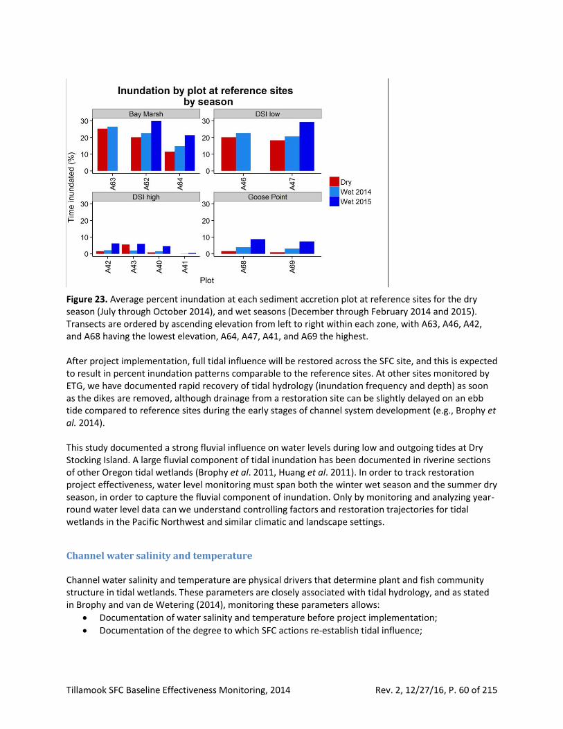
Tillamook SFC Baseline Effectiveness Monitoring, 2014 Rev. 2, 12/27/16, P. 60 of 215
Figure 23. Average percent inundation at each sediment accretion plot at reference sites for the dry season (July through October 2014), and wet seasons (December through February 2014 and 2015). Transects are ordered by ascending elevation from left to right within each zone, with A63, A46, A42, and A68 having the lowest elevation, A64, A47, A41, and A69 the highest. After project implementation, full tidal influence will be restored across the SFC site, and this is expected to result in percent inundation patterns comparable to the reference sites. At other sites monitored by ETG, we have documented rapid recovery of tidal hydrology (inundation frequency and depth) as soon as the dikes are removed, although drainage from a restoration site can be slightly delayed on an ebb tide compared to reference sites during the early stages of channel system development (e.g., Brophy et al. 2014). This study documented a strong fluvial influence on water levels during low and outgoing tides at Dry Stocking Island. A large fluvial component of tidal inundation has been documented in riverine sections of other Oregon tidal wetlands (Brophy et al. 2011, Huang et al. 2011). In order to track restoration project effectiveness, water level monitoring must span both the winter wet season and the summer dry season, in order to capture the fluvial component of inundation. Only by monitoring and analyzing year-round water level data can we understand controlling factors and restoration trajectories for tidal wetlands in the Pacific Northwest and similar climatic and landscape settings.
Channel water salinity and temperature Channel water salinity and temperature are physical drivers that determine plant and fish community structure in tidal wetlands. These parameters are closely associated with tidal hydrology, and as stated in Brophy and van de Wetering (2014), monitoring these parameters allows:
• Documentation of water salinity and temperature before project implementation;
• Documentation of the degree to which SFC actions re-establish tidal influence;

Tillamook SFC Baseline Effectiveness Monitoring, 2014 Rev. 2, 12/27/16, P. 61 of 215
• Data on controlling factors, to assist interpretation of other monitoring results such as plant communities and fish populations. Changes in salinity and temperature are expected to related closely to post-implementation trajectory for these and other parameters.
Methods Channel water salinity and temperature were measured using Odyssey conductivity-temperature data-loggers programmed to collect data at 15 minute intervals. Monitoring began in late October 2013 and continued until February 2015. Loggers were co-located with water level loggers (Table 20, Maps A12 and A16-A17), and placed at the same elevation as the water level loggers (approximately MTL). Details of specific logger locations are provided in “Wetland surface elevation and water level: Methods” above. Using data from the water level loggers, data were “trimmed” when conductivity-temperature loggers were out of the water. Raw logger data were converted from conductivity values to salinity values using a calibration formula determined for each individual logger. Loggers were calibrated before and after each deployment period using a multi-point conductivity and temperature calibration procedure, and the resulting calibration formula was deployment-specific. Daily maximum salinity and temperature were extracted from the 15 minute interval data. Statistical analysis of daily maximum salinity and temperature was conducted for four analysis periods: winter (12/1/13 - 2/17/14 and 12/1/14 - 2/17/15), early spring (3/1/14 - 4/30/14), late spring (5/1/14 - 5/20/14), and summer (7/23/14 - 8/1/14) (Table 20). These seasons were selected to correlate with the analyses presented in the Fish use, prey resources, and habitat section, and were limited to relatively short time periods with continuous data coverage for all loggers included in the analysis, to ensure data comparability across locations. The analysis for each season included all loggers except those that were out of the water for significant amounts of time during the analysis period; excluded loggers are shown in Table 20. Seasonal differences in average daily maximum salinity and temperature between the SFC site and reference sites were determined using a t-test. Seasonal differences among logger sites were tested using a 1 way ANOVA. When distributions did not meet the normality assumptions, an equivalent non-parametric test was used (either a Wilcoxon in place of a t-test or Kruskal-Wallis in place of ANOVA). All analyses were completed in R (Version 3.1.1). Table 20. Dates and tidal hydrology/water quality loggers used for each seasonal analysis. All loggers were included in the analysis for each period, except those shown in the “loggers excluded” column. Loggers were excluded when they were out of the water for a significant amount of time during the analysis period.
Season Dates Loggers excluded
Winter 12/1/13-2/17/14 & 12/1/14-2/17/15 none
Early spring 3/1/14-4/30/14 none
Late spring 5/1/14-5/20/14 Blind Slough Road Blind Slough Upper
Summer 7/23/14-8/1/14
Goose Point Nolan Slough Blind Slough Upper Blind Slough Mid Trib upper
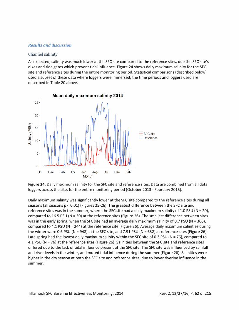
Tillamook SFC Baseline Effectiveness Monitoring, 2014 Rev. 2, 12/27/16, P. 62 of 215
Results and discussion
Channel salinity
As expected, salinity was much lower at the SFC site compared to the reference sites, due the SFC site’s dikes and tide gates which prevent tidal influence. Figure 24 shows daily maximum salinity for the SFC site and reference sites during the entire monitoring period. Statistical comparisons (described below) used a subset of these data where loggers were immersed; the time periods and loggers used are described in Table 20 above.
Figure 24. Daily maximum salinity for the SFC site and reference sites. Data are combined from all data loggers across the site, for the entire monitoring period (October 2013 - February 2015). Daily maximum salinity was significantly lower at the SFC site compared to the reference sites during all seasons (all seasons p < 0.01) (Figures 25-26). The greatest difference between the SFC site and reference sites was in the summer, where the SFC site had a daily maximum salinity of 1.0 PSU (N = 20), compared to 16.5 PSU (N = 30) at the reference sites (Figure 26). The smallest difference between sites was in the early spring, when the SFC site had an average daily maximum salinity of 0.7 PSU (N = 366), compared to 4.1 PSU (N = 244) at the reference site (Figure 26). Average daily maximum salinities during the winter were 0.6 PSU (N = 948) at the SFC site, and 7.91 PSU (N = 632) at reference sites (Figure 26). Late spring had the lowest daily maximum salinity within the SFC site of 0.3 PSU (N = 76), compared to 4.1 PSU (N = 76) at the reference sites (Figure 26). Salinities between the SFC site and reference sites differed due to the lack of tidal influence present at the SFC site. The SFC site was influenced by rainfall and river levels in the winter, and muted tidal influence during the summer (Figure 26). Salinities were higher in the dry season at both the SFC site and reference sites, due to lower riverine influence in the summer.
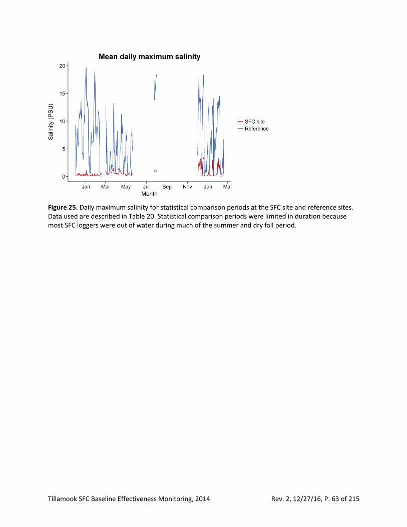
Tillamook SFC Baseline Effectiveness Monitoring, 2014 Rev. 2, 12/27/16, P. 63 of 215
Figure 25. Daily maximum salinity for statistical comparison periods at the SFC site and reference sites. Data used are described in Table 20. Statistical comparison periods were limited in duration because most SFC loggers were out of water during much of the summer and dry fall period.
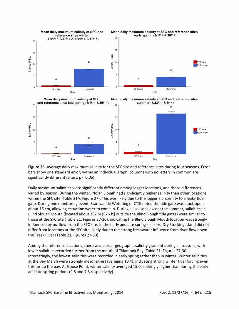
Tillamook SFC Baseline Effectiveness Monitoring, 2014 Rev. 2, 12/27/16, P. 64 of 215
Figure 26. Average daily maximum salinity for the SFC site and reference sites during four seasons. Error bars show one standard error; within an individual graph, columns with no letters in common are significantly different (t-test, p < 0.05). Daily maximum salinities were significantly different among logger locations, and those differences varied by season. During the winter, Nolan Slough had significantly higher salinity than other locations within the SFC site (Table 21A, Figure 27). This was likely due to the logger’s proximity to a leaky tide gate. During one monitoring event, Stan van de Wetering of CTSI noted the tide gate was stuck open about 15 cm, allowing estuarine water to come in. During all seasons except the summer, salinities at Blind Slough Mouth (located about 267 m [875 ft] outside the Blind Slough tide gates) were similar to those at the SFC site (Table 21, Figures 27-30), indicating the Blind Slough Mouth location was strongly influenced by outflow from the SFC site. In the early and late spring seasons, Dry Stocking Island did not differ from locations at the SFC site, likely due to the strong freshwater influence from river flow down the Trask River (Table 21, Figures 27-30). Among the reference locations, there was a clear geographic salinity gradient during all seasons, with lower salinities recorded further from the mouth of Tillamook Bay (Table 21, Figures 27-30). Interestingly, the lowest salinities were recorded in early spring rather than in winter. Winter salinities at the Bay Marsh were strongly mesohaline (averaging 10.4), indicating strong winter tidal forcing even this far up the bay. At Goose Point, winter salinity averaged 15.0, strikingly higher than during the early and late spring periods (9.8 and 7.3 respectively).
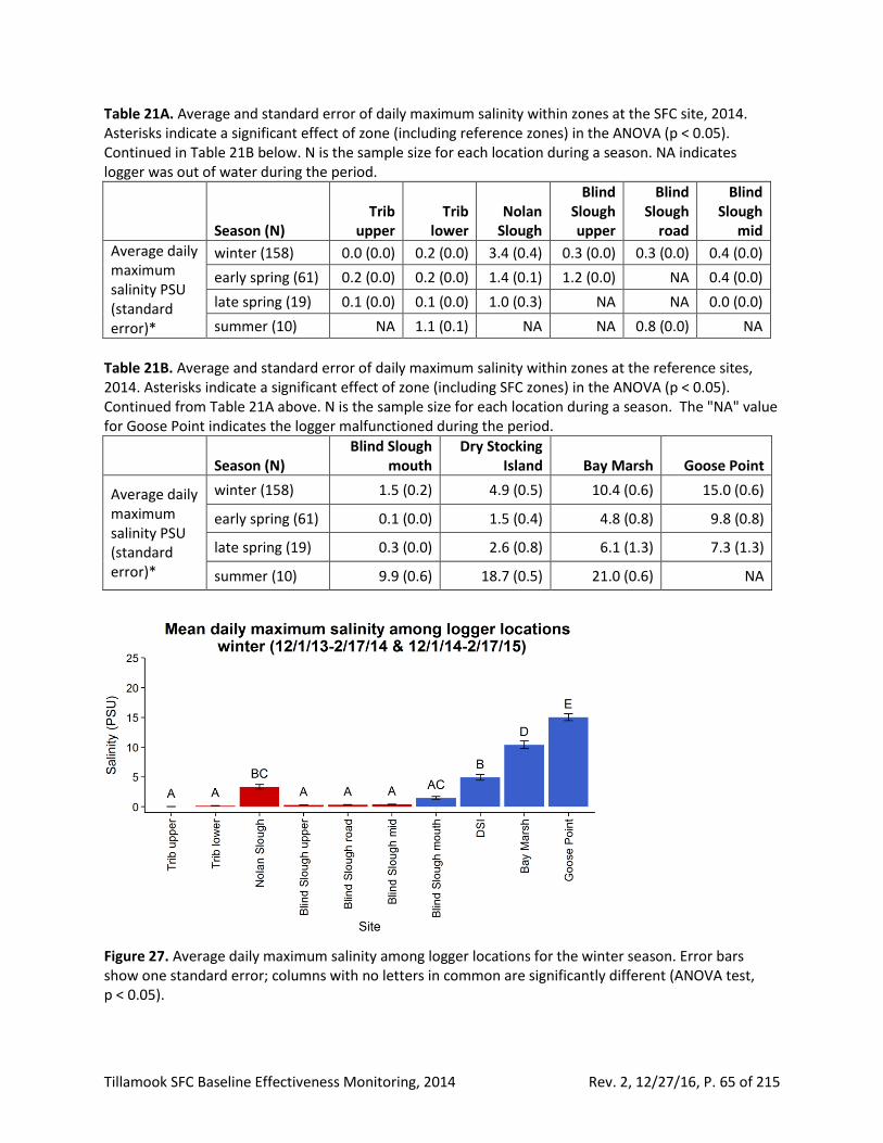
Tillamook SFC Baseline Effectiveness Monitoring, 2014 Rev. 2, 12/27/16, P. 65 of 215
Table 21A. Average and standard error of daily maximum salinity within zones at the SFC site, 2014. Asterisks indicate a significant effect of zone (including reference zones) in the ANOVA (p < 0.05). Continued in Table 21B below. N is the sample size for each location during a season. NA indicates logger was out of water during the period.
Season (N) Trib
upper Trib
lower Nolan
Slough
Blind Slough upper
Blind Slough
road
Blind Slough
mid
Average daily maximum salinity PSU (standard error)*
winter (158) 0.0 (0.0) 0.2 (0.0) 3.4 (0.4) 0.3 (0.0) 0.3 (0.0) 0.4 (0.0)
early spring (61) 0.2 (0.0) 0.2 (0.0) 1.4 (0.1) 1.2 (0.0) NA 0.4 (0.0)
late spring (19) 0.1 (0.0) 0.1 (0.0) 1.0 (0.3) NA NA 0.0 (0.0)
summer (10) NA 1.1 (0.1) NA NA 0.8 (0.0) NA
Table 21B. Average and standard error of daily maximum salinity within zones at the reference sites, 2014. Asterisks indicate a significant effect of zone (including SFC zones) in the ANOVA (p < 0.05). Continued from Table 21A above. N is the sample size for each location during a season. The "NA" value for Goose Point indicates the logger malfunctioned during the period.
Season (N) Blind Slough
mouth Dry Stocking
Island Bay Marsh Goose Point
Average daily maximum salinity PSU (standard error)*
winter (158) 1.5 (0.2) 4.9 (0.5) 10.4 (0.6) 15.0 (0.6)
early spring (61) 0.1 (0.0) 1.5 (0.4) 4.8 (0.8) 9.8 (0.8)
late spring (19) 0.3 (0.0) 2.6 (0.8) 6.1 (1.3) 7.3 (1.3)
summer (10) 9.9 (0.6) 18.7 (0.5) 21.0 (0.6) NA
Figure 27. Average daily maximum salinity among logger locations for the winter season. Error bars show one standard error; columns with no letters in common are significantly different (ANOVA test, p < 0.05).
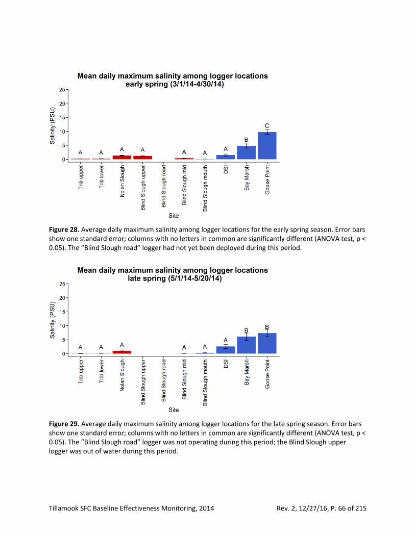
Tillamook SFC Baseline Effectiveness Monitoring, 2014 Rev. 2, 12/27/16, P. 66 of 215
Figure 28. Average daily maximum salinity among logger locations for the early spring season. Error bars show one standard error; columns with no letters in common are significantly different (ANOVA test, p < 0.05). The “Blind Slough road” logger had not yet been deployed during this period.
Figure 29. Average daily maximum salinity among logger locations for the late spring season. Error bars show one standard error; columns with no letters in common are significantly different (ANOVA test, p < 0.05). The “Blind Slough road” logger was not operating during this period; the Blind Slough upper logger was out of water during this period.
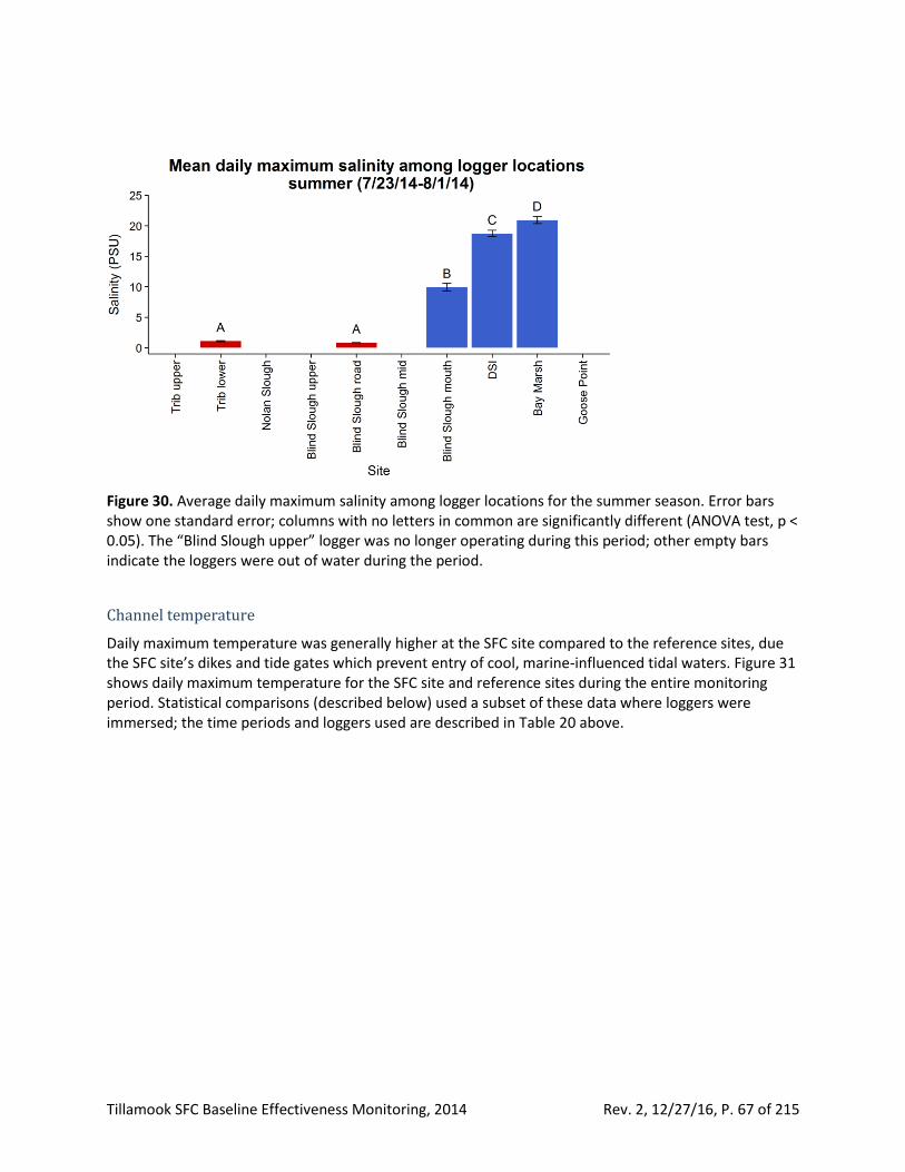
Tillamook SFC Baseline Effectiveness Monitoring, 2014 Rev. 2, 12/27/16, P. 67 of 215
Figure 30. Average daily maximum salinity among logger locations for the summer season. Error bars show one standard error; columns with no letters in common are significantly different (ANOVA test, p < 0.05). The “Blind Slough upper” logger was no longer operating during this period; other empty bars indicate the loggers were out of water during the period.
Channel temperature
Daily maximum temperature was generally higher at the SFC site compared to the reference sites, due the SFC site’s dikes and tide gates which prevent entry of cool, marine-influenced tidal waters. Figure 31 shows daily maximum temperature for the SFC site and reference sites during the entire monitoring period. Statistical comparisons (described below) used a subset of these data where loggers were immersed; the time periods and loggers used are described in Table 20 above.
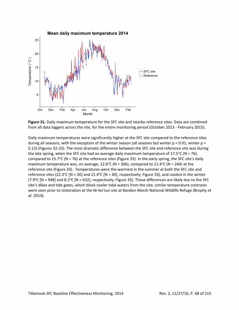
Tillamook SFC Baseline Effectiveness Monitoring, 2014 Rev. 2, 12/27/16, P. 68 of 215
Figure 31. Daily maximum temperature for the SFC site and nearby reference sites. Data are combined from all data loggers across the site, for the entire monitoring period (October 2013 - February 2015). Daily maximum temperatures were significantly higher at the SFC site compared to the reference sites during all seasons, with the exception of the winter season (all seasons but winter p < 0.01; winter p = 0.13) (Figures 32-33). The most dramatic difference between the SFC site and reference site was during the late spring, when the SFC site had an average daily maximum temperature of 17.5oC (N = 76), compared to 15.7oC (N = 76) at the reference sites (Figure 33). In the early spring, the SFC site’s daily maximum temperature was, on average, 12.6oC (N = 366), compared to 11.4oC (N = 244) at the reference site (Figure 33). Temperatures were the warmest in the summer at both the SFC site and reference sites (22.3oC [N = 20] and 21.4oC [N = 30], respectively; Figure 33), and coolest in the winter (7.9oC [N = 948] and 8.2oC [N = 632], respectively; Figure 33). These differences are likely due to the SFC site’s dikes and tide gates, which block cooler tidal waters from the site; similar temperature contrasts were seen prior to restoration at the Ni-les’tun site at Bandon Marsh National Wildlife Refuge (Brophy et al. 2014).
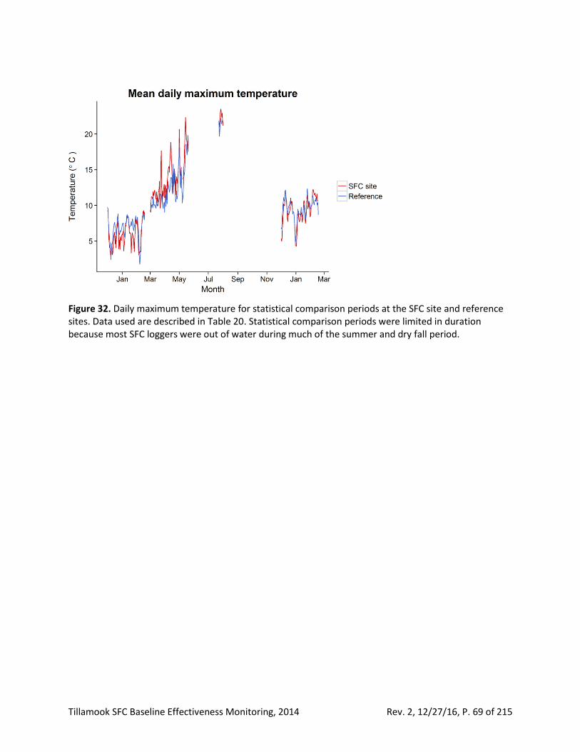
Tillamook SFC Baseline Effectiveness Monitoring, 2014 Rev. 2, 12/27/16, P. 69 of 215
Figure 32. Daily maximum temperature for statistical comparison periods at the SFC site and reference sites. Data used are described in Table 20. Statistical comparison periods were limited in duration because most SFC loggers were out of water during much of the summer and dry fall period.
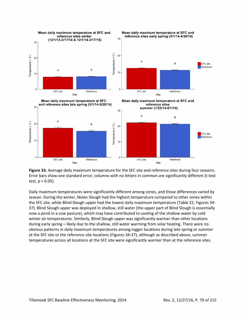
Tillamook SFC Baseline Effectiveness Monitoring, 2014 Rev. 2, 12/27/16, P. 70 of 215
Figure 33. Average daily maximum temperature for the SFC site and reference sites during four seasons. Error bars show one standard error; columns with no letters in common are significantly different (t-test test, p < 0.05). Daily maximum temperatures were significantly different among zones, and those differences varied by season. During the winter, Nolan Slough had the highest temperature compared to other zones within the SFC site, while Blind Slough upper had the lowest daily maximum temperature (Table 22, Figures 34-37). Blind Slough upper was deployed in shallow, still water (the upper part of Blind Slough is essentially now a pond in a cow pasture), which may have contributed to cooling of the shallow water by cold winter air temperatures. Similarly, Blind Slough upper was significantly warmer than other locations during early spring – likely due to the shallow, still water warming from solar heating. There were no obvious patterns in daily maximum temperatures among logger locations during late spring or summer at the SFC site or the reference site locations (Figures 34-37), although as described above, summer temperatures across all locations at the SFC site were significantly warmer than at the reference sites.
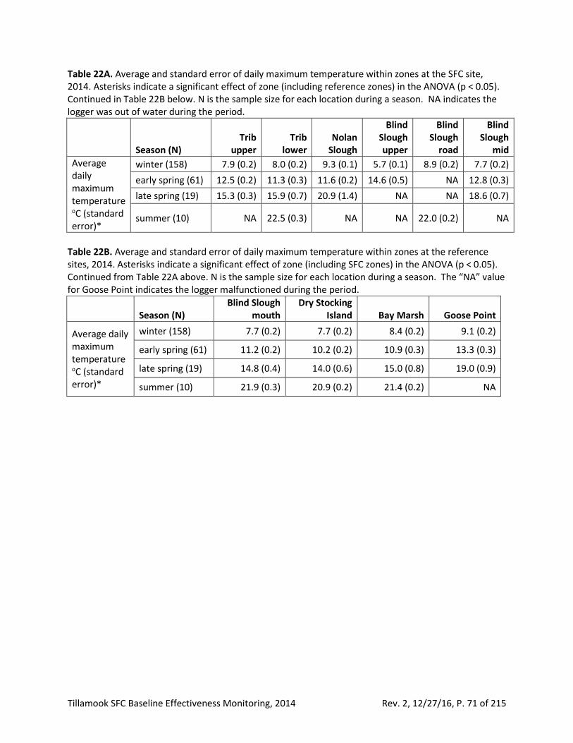
Tillamook SFC Baseline Effectiveness Monitoring, 2014 Rev. 2, 12/27/16, P. 71 of 215
Table 22A. Average and standard error of daily maximum temperature within zones at the SFC site, 2014. Asterisks indicate a significant effect of zone (including reference zones) in the ANOVA (p < 0.05). Continued in Table 22B below. N is the sample size for each location during a season. NA indicates the logger was out of water during the period.
Season (N) Trib
upper Trib
lower Nolan
Slough
Blind Slough upper
Blind Slough
road
Blind Slough
mid
Average daily maximum temperature oC (standard error)*
winter (158) 7.9 (0.2) 8.0 (0.2) 9.3 (0.1) 5.7 (0.1) 8.9 (0.2) 7.7 (0.2)
early spring (61) 12.5 (0.2) 11.3 (0.3) 11.6 (0.2) 14.6 (0.5) NA 12.8 (0.3)
late spring (19) 15.3 (0.3) 15.9 (0.7) 20.9 (1.4) NA NA 18.6 (0.7)
summer (10) NA 22.5 (0.3) NA NA 22.0 (0.2) NA
Table 22B. Average and standard error of daily maximum temperature within zones at the reference sites, 2014. Asterisks indicate a significant effect of zone (including SFC zones) in the ANOVA (p < 0.05). Continued from Table 22A above. N is the sample size for each location during a season. The “NA” value for Goose Point indicates the logger malfunctioned during the period.
Season (N) Blind Slough
mouth Dry Stocking
Island Bay Marsh Goose Point
Average daily maximum temperature oC (standard error)*
winter (158) 7.7 (0.2) 7.7 (0.2) 8.4 (0.2) 9.1 (0.2)
early spring (61) 11.2 (0.2) 10.2 (0.2) 10.9 (0.3) 13.3 (0.3)
late spring (19) 14.8 (0.4) 14.0 (0.6) 15.0 (0.8) 19.0 (0.9)
summer (10) 21.9 (0.3) 20.9 (0.2) 21.4 (0.2) NA
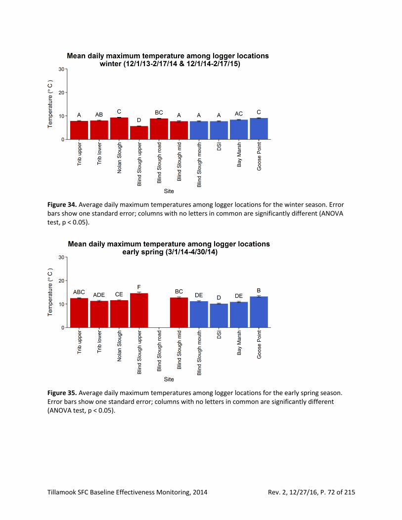
Tillamook SFC Baseline Effectiveness Monitoring, 2014 Rev. 2, 12/27/16, P. 72 of 215
Figure 34. Average daily maximum temperatures among logger locations for the winter season. Error bars show one standard error; columns with no letters in common are significantly different (ANOVA test, p < 0.05).
Figure 35. Average daily maximum temperatures among logger locations for the early spring season. Error bars show one standard error; columns with no letters in common are significantly different (ANOVA test, p < 0.05).
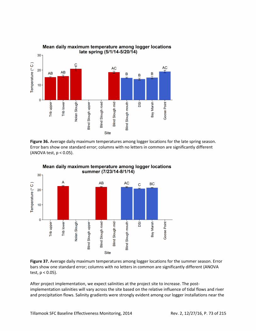
Tillamook SFC Baseline Effectiveness Monitoring, 2014 Rev. 2, 12/27/16, P. 73 of 215
Figure 36. Average daily maximum temperatures among logger locations for the late spring season. Error bars show one standard error; columns with no letters in common are significantly different (ANOVA test, p < 0.05).
Figure 37. Average daily maximum temperatures among logger locations for the summer season. Error bars show one standard error; columns with no letters in common are significantly different (ANOVA test, p < 0.05). After project implementation, we expect salinities at the project site to increase. The post-implementation salinities will vary across the site based on the relative influence of tidal flows and river and precipitation flows. Salinity gradients were strongly evident among our logger installations near the
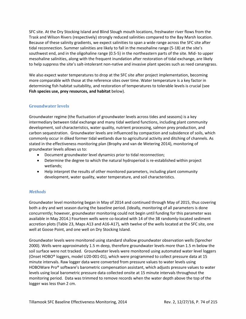
Tillamook SFC Baseline Effectiveness Monitoring, 2014 Rev. 2, 12/27/16, P. 74 of 215
SFC site. At the Dry Stocking Island and Blind Slough mouth locations, freshwater river flows from the Trask and Wilson Rivers (respectively) strongly reduced salinities compared to the Bay Marsh location. Because of these salinity gradients, we expect salinities to span a wide range across the SFC site after tidal reconnection. Summer salinities are likely to fall in the mesohaline range (5-18) at the site’s southwest end, and in the oligohaline range (0.5-5) in the northeastern parts of the site. Mid- to upper mesohaline salinities, along with the frequent inundation after restoration of tidal exchange, are likely to help suppress the site’s salt-intolerant non-native and invasive plant species such as reed canarygrass. We also expect water temperatures to drop at the SFC site after project implementation, becoming more comparable with those at the reference sites over time. Water temperature is a key factor in determining fish habitat suitability, and restoration of temperatures to tolerable levels is crucial (see Fish species use, prey resources, and habitat below).
Groundwater levels Groundwater regime (the fluctuation of groundwater levels across tides and seasons) is a key intermediary between tidal exchange and many tidal wetland functions, including plant community development, soil characteristics, water quality, nutrient processing, salmon prey production, and carbon sequestration. Groundwater levels are influenced by compaction and subsidence of soils, which commonly occur in diked former tidal wetlands due to agricultural activity and ditching of channels. As stated in the effectiveness monitoring plan (Brophy and van de Wetering 2014), monitoring of groundwater levels allows us to:
• Document groundwater level dynamics prior to tidal reconnection;
• Determine the degree to which the natural hydroperiod is re-established within project wetlands;
• Help interpret the results of other monitored parameters, including plant community development, water quality, water temperature, and soil characteristics.
Methods Groundwater level monitoring began in May of 2014 and continued through May of 2015, thus covering both a dry and wet season during the baseline period. (Ideally, monitoring of all parameters is done concurrently; however, groundwater monitoring could not begin until funding for this parameter was available in May 2014.) Fourteen wells were co-located with 14 of the 38 randomly-located sediment accretion plots (Table 23, Maps A13 and A16-A17), with twelve of the wells located at the SFC site, one well at Goose Point, and one well on Dry Stocking Island. Groundwater levels were monitored using standard shallow groundwater observation wells (Sprecher 2000). Wells were approximately 1.5 m deep, therefore groundwater levels more than 1.5 m below the soil surface were not tracked. Groundwater levels were monitored using automated water level loggers (Onset HOBO® loggers, model U20-001-01), which were programmed to collect pressure data at 15 minute intervals. Raw logger data were converted from pressure values to water levels using HOBOWare Pro® software’s barometric compensation assistant, which adjusts pressure values to water levels using local barometric pressure data collected onsite at 15 minute intervals throughout the monitoring period. Data was trimmed to remove records when the water depth above the top of the logger was less than 2 cm.
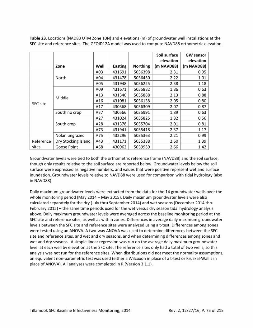
Tillamook SFC Baseline Effectiveness Monitoring, 2014 Rev. 2, 12/27/16, P. 75 of 215
Table 23. Locations (NAD83 UTM Zone 10N) and elevations (m) of groundwater well installations at the SFC site and reference sites. The GEOID12A model was used to compute NAVD88 orthometric elevation.
Zone Well Easting Northing
Soil surface elevation
(m NAVD88)
GW sensor elevation
(m NAVD88)
SFC site
North
A03 431691 5036398 2.31 0.95
A04 431478 5036430 2.22 1.01
A05 431948 5036225 2.38 1.18
Middle
A09 431671 5035882 1.86 0.63
A13 431340 5035888 2.13 0.88
A16 431081 5036138 2.05 0.80
A17 430368 5036309 2.07 0.87
South no crop A37 430566 5035991 1.89 0.63
South crop
A27 431024 5035825 1.82 0.56
A28 431378 5035704 2.01 0.81
A73 431941 5035418 2.37 1.17
Nolan ungrazed A75 432296 5035363 2.21 0.99
Reference sites
Dry Stocking Island A43 431171 5035388 2.60 1.39
Goose Point A68 430962 5039939 2.66 1.42
Groundwater levels were tied to both the orthometric reference frame (NAVD88) and the soil surface, though only results relative to the soil surface are reported below. Groundwater levels below the soil surface were expressed as negative numbers, and values that were positive represent wetland surface inundation. Groundwater levels relative to NAVD88 were used for comparison with tidal hydrology (also in NAVD88). Daily maximum groundwater levels were extracted from the data for the 14 groundwater wells over the whole monitoring period (May 2014 – May 2015). Daily maximum groundwater levels were also calculated separately for the dry (July thru September 2014) and wet seasons (December 2014 thru February 2015) – the same time periods used for the wet versus dry season tidal hydrology analysis above. Daily maximum groundwater levels were averaged across the baseline monitoring period at the SFC site and reference sites, as well as within zones. Differences in average daily maximum groundwater levels between the SFC site and reference sites were analyzed using a t-test. Differences among zones were tested using an ANOVA. A two-way ANOVA was used to determine differences between the SFC site and reference sites, and wet and dry seasons, and when determining differences among zones and wet and dry seasons. A simple linear regression was run on the average daily maximum groundwater level at each well by elevation at the SFC site. The reference sites only had a total of two wells, so this analysis was not run for the reference sites. When distributions did not meet the normality assumptions, an equivalent non-parametric test was used (either a Wilcoxon in place of a t-test or Kruskal-Wallis in place of ANOVA). All analyses were completed in R (Version 3.1.1).
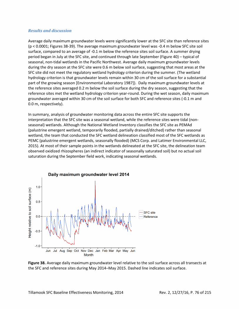
Tillamook SFC Baseline Effectiveness Monitoring, 2014 Rev. 2, 12/27/16, P. 76 of 215
Results and discussion Average daily maximum groundwater levels were significantly lower at the SFC site than reference sites (p < 0.0001; Figures 38-39). The average maximum groundwater level was -0.4 m below SFC site soil surface, compared to an average of -0.1 m below the reference sites soil surface. A summer drying period began in July at the SFC site, and continued through late September (Figure 40) – typical of seasonal, non-tidal wetlands in the Pacific Northwest. Average daily maximum groundwater levels during the dry season at the SFC site were 0.6 m below soil surface, suggesting that most areas at the SFC site did not meet the regulatory wetland hydrology criterion during the summer. (The wetland hydrology criterion is that groundwater levels remain within 30 cm of the soil surface for a substantial part of the growing season [Environmental Laboratory 1987]). Daily maximum groundwater levels at the reference sites averaged 0.2 m below the soil surface during the dry season, suggesting that the reference sites met the wetland hydrology criterion year-round. During the wet season, daily maximum groundwater averaged within 30 cm of the soil surface for both SFC and reference sites (-0.1 m and 0.0 m, respectively). In summary, analysis of groundwater monitoring data across the entire SFC site supports the interpretation that the SFC site was a seasonal wetland, while the reference sites were tidal (non-seasonal) wetlands. Although the National Wetland Inventory classifies the SFC site as PEMAd (palustrine emergent wetland, temporarily flooded, partially drained/ditched) rather than seasonal wetland, the team that conducted the SFC wetland delineation classified most of the SFC wetlands as PEMC (palustrine emergent wetlands, seasonally flooded) (MCS Corp. and Latimer Environmental LLC, 2015). At most of their sample points in the wetlands delineated at the SFC site, the delineation team observed oxidized rhizospheres (an indirect indicator of seasonally saturated soil) but no actual soil saturation during the September field work, indicating seasonal wetlands.
Figure 38. Average daily maximum groundwater level relative to the soil surface across all transects at the SFC and reference sites during May 2014–May 2015. Dashed line indicates soil surface.
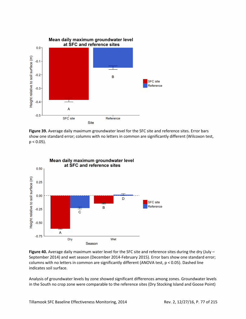
Tillamook SFC Baseline Effectiveness Monitoring, 2014 Rev. 2, 12/27/16, P. 77 of 215
Figure 39. Average daily maximum groundwater level for the SFC site and reference sites. Error bars show one standard error; columns with no letters in common are significantly different (Wilcoxon test, p < 0.05).
Figure 40. Average daily maximum water level for the SFC site and reference sites during the dry (July – September 2014) and wet season (December 2014-February 2015). Error bars show one standard error; columns with no letters in common are significantly different (ANOVA test, p < 0.05). Dashed line indicates soil surface. Analysis of groundwater levels by zone showed significant differences among zones. Groundwater levels in the South no crop zone were comparable to the reference sites (Dry Stocking Island and Goose Point)
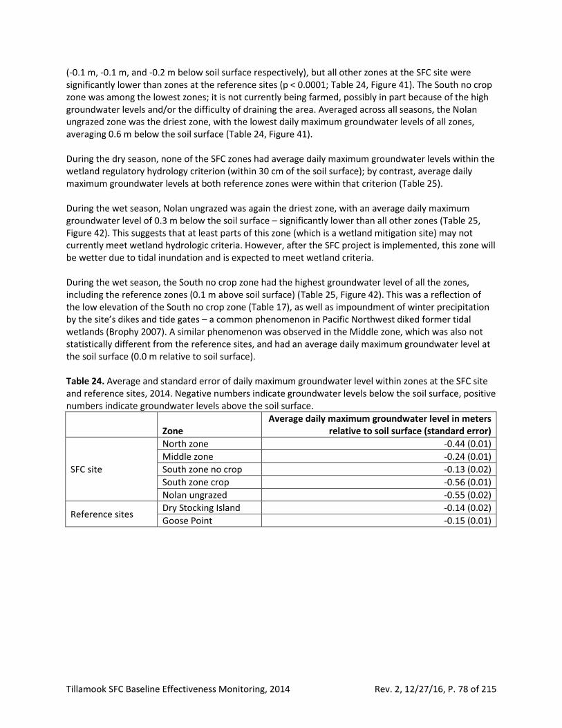
Tillamook SFC Baseline Effectiveness Monitoring, 2014 Rev. 2, 12/27/16, P. 78 of 215
(-0.1 m, -0.1 m, and -0.2 m below soil surface respectively), but all other zones at the SFC site were significantly lower than zones at the reference sites (p < 0.0001; Table 24, Figure 41). The South no crop zone was among the lowest zones; it is not currently being farmed, possibly in part because of the high groundwater levels and/or the difficulty of draining the area. Averaged across all seasons, the Nolan ungrazed zone was the driest zone, with the lowest daily maximum groundwater levels of all zones, averaging 0.6 m below the soil surface (Table 24, Figure 41). During the dry season, none of the SFC zones had average daily maximum groundwater levels within the wetland regulatory hydrology criterion (within 30 cm of the soil surface); by contrast, average daily maximum groundwater levels at both reference zones were within that criterion (Table 25). During the wet season, Nolan ungrazed was again the driest zone, with an average daily maximum groundwater level of 0.3 m below the soil surface – significantly lower than all other zones (Table 25, Figure 42). This suggests that at least parts of this zone (which is a wetland mitigation site) may not currently meet wetland hydrologic criteria. However, after the SFC project is implemented, this zone will be wetter due to tidal inundation and is expected to meet wetland criteria. During the wet season, the South no crop zone had the highest groundwater level of all the zones, including the reference zones (0.1 m above soil surface) (Table 25, Figure 42). This was a reflection of the low elevation of the South no crop zone (Table 17), as well as impoundment of winter precipitation by the site’s dikes and tide gates – a common phenomenon in Pacific Northwest diked former tidal wetlands (Brophy 2007). A similar phenomenon was observed in the Middle zone, which was also not statistically different from the reference sites, and had an average daily maximum groundwater level at the soil surface (0.0 m relative to soil surface). Table 24. Average and standard error of daily maximum groundwater level within zones at the SFC site and reference sites, 2014. Negative numbers indicate groundwater levels below the soil surface, positive numbers indicate groundwater levels above the soil surface.
Zone Average daily maximum groundwater level in meters
relative to soil surface (standard error)
SFC site
North zone -0.44 (0.01)
Middle zone -0.24 (0.01)
South zone no crop -0.13 (0.02)
South zone crop -0.56 (0.01)
Nolan ungrazed -0.55 (0.02)
Reference sites Dry Stocking Island -0.14 (0.02)
Goose Point -0.15 (0.01)
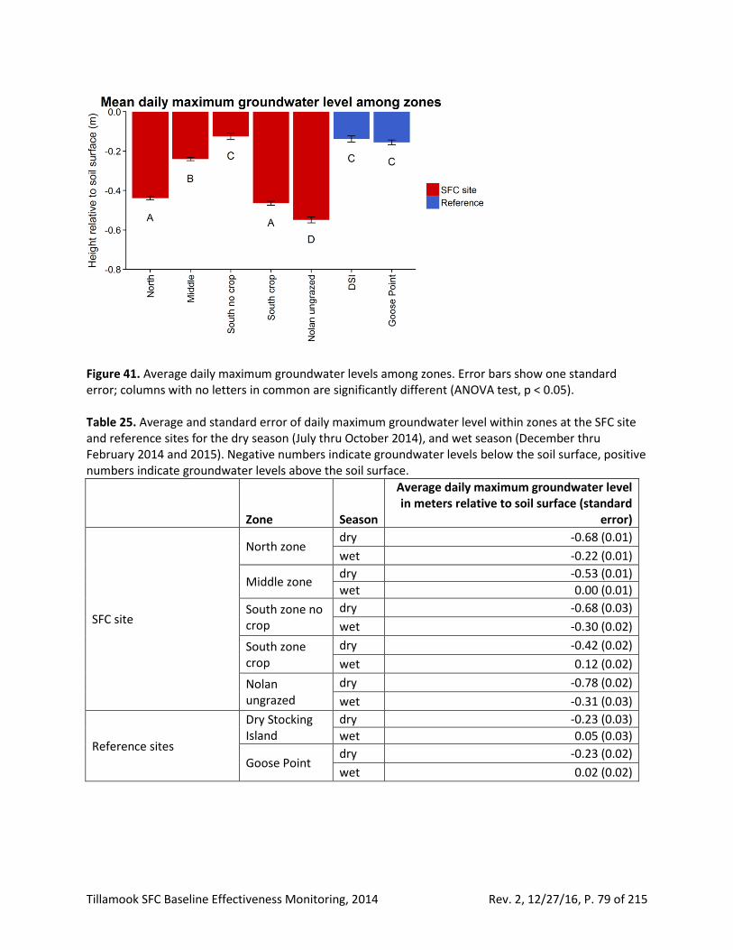
Tillamook SFC Baseline Effectiveness Monitoring, 2014 Rev. 2, 12/27/16, P. 79 of 215
Figure 41. Average daily maximum groundwater levels among zones. Error bars show one standard error; columns with no letters in common are significantly different (ANOVA test, p < 0.05). Table 25. Average and standard error of daily maximum groundwater level within zones at the SFC site and reference sites for the dry season (July thru October 2014), and wet season (December thru February 2014 and 2015). Negative numbers indicate groundwater levels below the soil surface, positive numbers indicate groundwater levels above the soil surface.
Zone Season
Average daily maximum groundwater level in meters relative to soil surface (standard
error)
SFC site
North zone dry -0.68 (0.01)
wet -0.22 (0.01)
Middle zone dry -0.53 (0.01)
wet 0.00 (0.01)
South zone no crop
dry -0.68 (0.03)
wet -0.30 (0.02)
South zone crop
dry -0.42 (0.02)
wet 0.12 (0.02)
Nolan ungrazed
dry -0.78 (0.02)
wet -0.31 (0.03)
Reference sites
Dry Stocking Island
dry -0.23 (0.03)
wet 0.05 (0.03)
Goose Point dry -0.23 (0.02)
wet 0.02 (0.02)
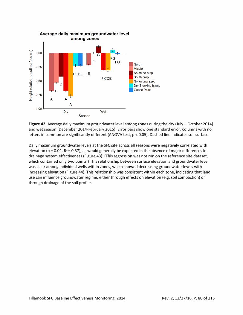
Tillamook SFC Baseline Effectiveness Monitoring, 2014 Rev. 2, 12/27/16, P. 80 of 215
Figure 42. Average daily maximum groundwater level among zones during the dry (July – October 2014) and wet season (December 2014-February 2015). Error bars show one standard error; columns with no letters in common are significantly different (ANOVA test, p < 0.05). Dashed line indicates soil surface. Daily maximum groundwater levels at the SFC site across all seasons were negatively correlated with elevation (p = 0.02, R2 = 0.37), as would generally be expected in the absence of major differences in drainage system effectiveness (Figure 43). (This regression was not run on the reference site dataset, which contained only two points.) This relationship between surface elevation and groundwater level was clear among individual wells within zones, which showed decreasing groundwater levels with increasing elevation (Figure 44). This relationship was consistent within each zone, indicating that land use can influence groundwater regime, either through effects on elevation (e.g. soil compaction) or through drainage of the soil profile.
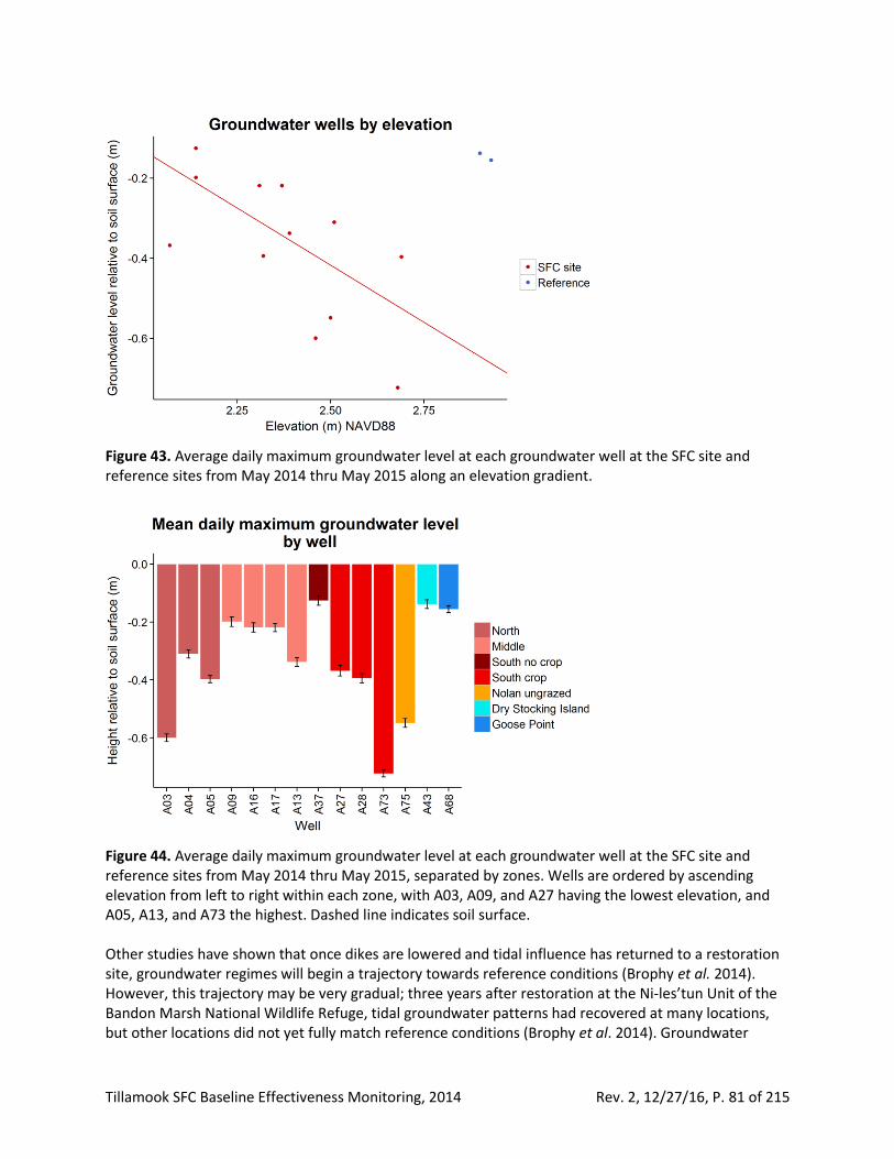
Tillamook SFC Baseline Effectiveness Monitoring, 2014 Rev. 2, 12/27/16, P. 81 of 215
Figure 43. Average daily maximum groundwater level at each groundwater well at the SFC site and reference sites from May 2014 thru May 2015 along an elevation gradient.
Figure 44. Average daily maximum groundwater level at each groundwater well at the SFC site and reference sites from May 2014 thru May 2015, separated by zones. Wells are ordered by ascending elevation from left to right within each zone, with A03, A09, and A27 having the lowest elevation, and A05, A13, and A73 the highest. Dashed line indicates soil surface. Other studies have shown that once dikes are lowered and tidal influence has returned to a restoration site, groundwater regimes will begin a trajectory towards reference conditions (Brophy et al. 2014). However, this trajectory may be very gradual; three years after restoration at the Ni-les’tun Unit of the Bandon Marsh National Wildlife Refuge, tidal groundwater patterns had recovered at many locations, but other locations did not yet fully match reference conditions (Brophy et al. 2014). Groundwater
Tillamook SFC Baseline Effectiveness Monitoring, 2014 Rev. 2, 12/27/16, P. 82 of 215
regimes may be affected by compaction, subsidence of soil, and tidal channel development, factors which may change slowly for many years after the re-establishment of tidal exchange (Brophy and van de Wetering 2012, Brophy et al. 2014).
Soils Soil characteristics, such as soil organic matter, soil organic carbon, soil pH, and soil salinity, are controlling factors for plant community development and are closely related to other wetland functions, such as carbon storage, nutrient cycling, and water temperature moderation. As stated in Brophy and van de Wetering (2014), results from soil monitoring are used to:
• Evaluate differences in soil characteristics before and after project implementation, relative to reference wetland conditions; and
• Help interpret the results of other monitored parameters, particularly plant community development.
Methods Soil samples were collected using a Dutch auger during the dry season (August 2014) from the surface rooting zone (0-20.3 cm or 0-8 in); samples were co-located with each sediment accretion plot (Table 37). At each plot, 8 random subsamples were pooled, bulked in the field, and then delivered to AgSource Laboratory in Umatilla, Oregon for analysis. At the lab, large roots were removed, samples were dried and homogenized, and a subsample was removed for analysis. Electrical conductivity and pH were measured using a conductance meter and pH meter, respectively. Percent organic matter was determined using the loss on ignition method (Craft et al. 1991), which involved burning the material in a muffle furnace for two hours at 360oC. Soil salinity was calculated using electrical conductivity and a standard formula (Fofonoff and Millard 1983). Carbon content was calculated using a conversion specific to high organic soils (0.68 x % organic matter) (Kasozi et al. 2009). Soil metrics (pH, soil salinity, organic matter, and carbon content) were compared between the SFC site and reference sites using a t-test, and among zones using an ANOVA test. A simple linear regression was used to determine the relationship between elevation and soil metrics at the SFC site and reference sites. When distributions did not meet the normality assumptions, an equivalent non-parametric test
was used (either a Wilcoxon in place of a t-test or Kruskal-Wallis in place of ANOVA).
Results and discussion Soil pH and soil salinity were both significantly lower at the SFC site versus the reference sites (p < 0.001 for both metrics; Figure 45). Average soil pH was 5.2 at the SFC site, and 5.8 at reference sites, while average soil salinity was 0.2 PSU at the SFC site and 7.1 PSU at the reference sites. The significant difference in soil salinity between the SFC site and reference sites was due to the lack of tidal influence at the SFC site (see Wetland surface elevation and water levels). Once the dikes and tide gates are removed, we expect to see an increase in soil salinity at the SFC site. Soil salinity is a strong controlling factor for plant community development, so we expect to see changes in plant communities at the SFC site with the reintroduction of tidal influence. Organic matter and carbon content were not statistically different between the SFC site and reference
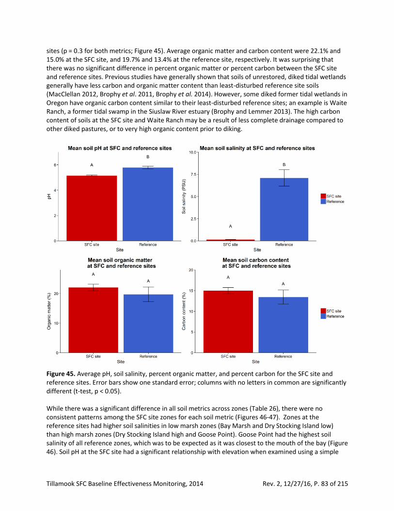
Tillamook SFC Baseline Effectiveness Monitoring, 2014 Rev. 2, 12/27/16, P. 83 of 215
sites (p = 0.3 for both metrics; Figure 45). Average organic matter and carbon content were 22.1% and 15.0% at the SFC site, and 19.7% and 13.4% at the reference site, respectively. It was surprising that there was no significant difference in percent organic matter or percent carbon between the SFC site and reference sites. Previous studies have generally shown that soils of unrestored, diked tidal wetlands generally have less carbon and organic matter content than least-disturbed reference site soils (MacClellan 2012, Brophy et al. 2011, Brophy et al. 2014). However, some diked former tidal wetlands in Oregon have organic carbon content similar to their least-disturbed reference sites; an example is Waite Ranch, a former tidal swamp in the Siuslaw River estuary (Brophy and Lemmer 2013). The high carbon content of soils at the SFC site and Waite Ranch may be a result of less complete drainage compared to other diked pastures, or to very high organic content prior to diking.
Figure 45. Average pH, soil salinity, percent organic matter, and percent carbon for the SFC site and reference sites. Error bars show one standard error; columns with no letters in common are significantly different (t-test, p < 0.05). While there was a significant difference in all soil metrics across zones (Table 26), there were no consistent patterns among the SFC site zones for each soil metric (Figures 46-47). Zones at the reference sites had higher soil salinities in low marsh zones (Bay Marsh and Dry Stocking Island low) than high marsh zones (Dry Stocking Island high and Goose Point). Goose Point had the highest soil salinity of all reference zones, which was to be expected as it was closest to the mouth of the bay (Figure 46). Soil pH at the SFC site had a significant relationship with elevation when examined using a simple
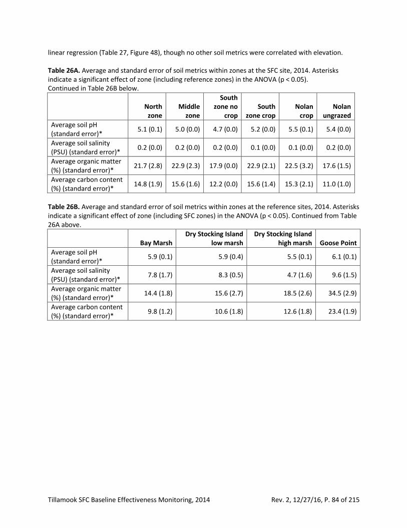
Tillamook SFC Baseline Effectiveness Monitoring, 2014 Rev. 2, 12/27/16, P. 84 of 215
linear regression (Table 27, Figure 48), though no other soil metrics were correlated with elevation. Table 26A. Average and standard error of soil metrics within zones at the SFC site, 2014. Asterisks indicate a significant effect of zone (including reference zones) in the ANOVA (p < 0.05). Continued in Table 26B below.
North
zone Middle
zone
South zone no
crop South
zone crop Nolan
crop Nolan
ungrazed
Average soil pH (standard error)*
5.1 (0.1) 5.0 (0.0) 4.7 (0.0) 5.2 (0.0) 5.5 (0.1) 5.4 (0.0)
Average soil salinity (PSU) (standard error)*
0.2 (0.0) 0.2 (0.0) 0.2 (0.0) 0.1 (0.0) 0.1 (0.0) 0.2 (0.0)
Average organic matter (%) (standard error)*
21.7 (2.8) 22.9 (2.3) 17.9 (0.0) 22.9 (2.1) 22.5 (3.2) 17.6 (1.5)
Average carbon content (%) (standard error)*
14.8 (1.9) 15.6 (1.6) 12.2 (0.0) 15.6 (1.4) 15.3 (2.1) 11.0 (1.0)
Table 26B. Average and standard error of soil metrics within zones at the reference sites, 2014. Asterisks indicate a significant effect of zone (including SFC zones) in the ANOVA (p < 0.05). Continued from Table 26A above.
Bay Marsh Dry Stocking Island
low marsh Dry Stocking Island
high marsh Goose Point
Average soil pH (standard error)*
5.9 (0.1) 5.9 (0.4) 5.5 (0.1) 6.1 (0.1)
Average soil salinity (PSU) (standard error)*
7.8 (1.7) 8.3 (0.5) 4.7 (1.6) 9.6 (1.5)
Average organic matter (%) (standard error)*
14.4 (1.8) 15.6 (2.7) 18.5 (2.6) 34.5 (2.9)
Average carbon content (%) (standard error)*
9.8 (1.2) 10.6 (1.8) 12.6 (1.8) 23.4 (1.9)
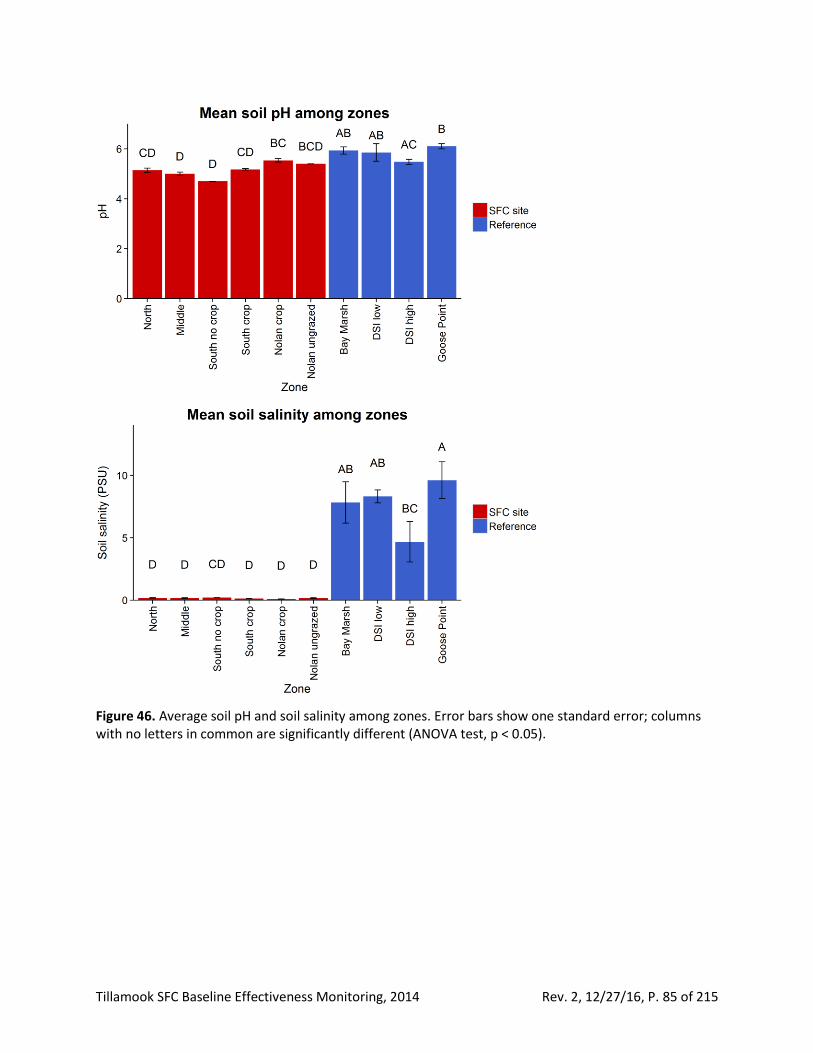
Tillamook SFC Baseline Effectiveness Monitoring, 2014 Rev. 2, 12/27/16, P. 85 of 215
Figure 46. Average soil pH and soil salinity among zones. Error bars show one standard error; columns with no letters in common are significantly different (ANOVA test, p < 0.05).
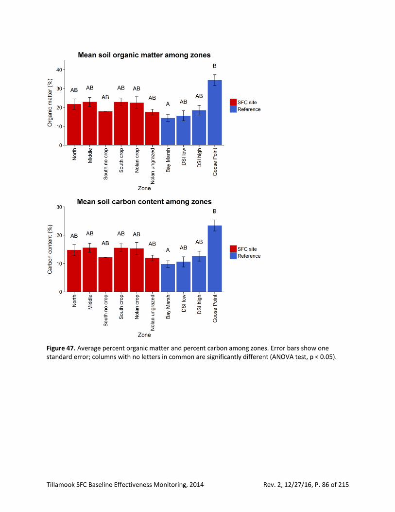
Tillamook SFC Baseline Effectiveness Monitoring, 2014 Rev. 2, 12/27/16, P. 86 of 215
Figure 47. Average percent organic matter and percent carbon among zones. Error bars show one standard error; columns with no letters in common are significantly different (ANOVA test, p < 0.05).
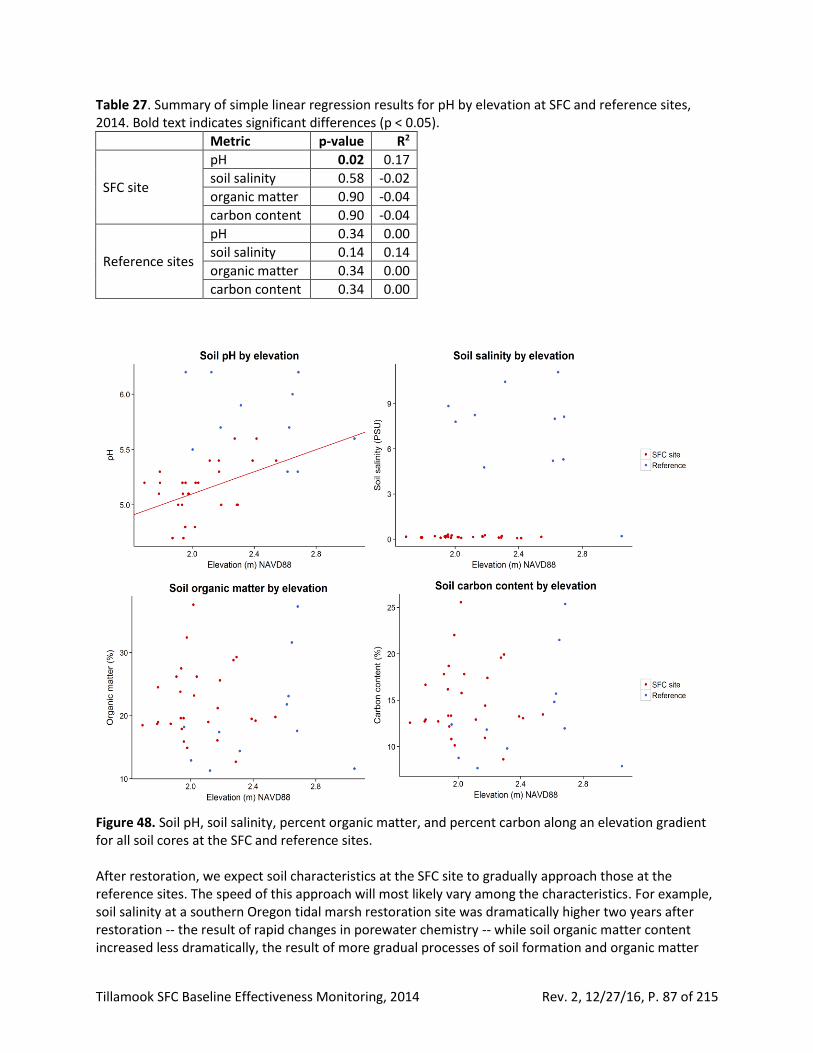
Tillamook SFC Baseline Effectiveness Monitoring, 2014 Rev. 2, 12/27/16, P. 87 of 215
Table 27. Summary of simple linear regression results for pH by elevation at SFC and reference sites, 2014. Bold text indicates significant differences (p < 0.05).
Metric p-value R2
SFC site
pH 0.02 0.17
soil salinity 0.58 -0.02
organic matter 0.90 -0.04
carbon content 0.90 -0.04
Reference sites
pH 0.34 0.00
soil salinity 0.14 0.14
organic matter 0.34 0.00
carbon content 0.34 0.00
Figure 48. Soil pH, soil salinity, percent organic matter, and percent carbon along an elevation gradient for all soil cores at the SFC and reference sites. After restoration, we expect soil characteristics at the SFC site to gradually approach those at the reference sites. The speed of this approach will most likely vary among the characteristics. For example, soil salinity at a southern Oregon tidal marsh restoration site was dramatically higher two years after restoration -- the result of rapid changes in porewater chemistry -- while soil organic matter content increased less dramatically, the result of more gradual processes of soil formation and organic matter
Tillamook SFC Baseline Effectiveness Monitoring, 2014 Rev. 2, 12/27/16, P. 88 of 215
accumulation (Brophy et al. 2014).
Channel morphology Channel morphology was monitored at the SFC site and reference sites to show differences between the two prior to project implementation. Channel geometry and development are expected to differ between sites of different channel drainage area, geomorphic settings, hydrology, disturbance, and land use history (Hood 2002, 2007; Diefenderfer et al. 2008, Ewald and Brophy 2012, Brophy 2007). As stated in Brophy and van de Wetering (2014), channel morphology measurements at the site will be used to:
• Evaluate channel morphology characteristics before SFC project implementation, and changes after implementation, relative to reference site channels;
• Quantify in-stream habitat;
• Quantify effects of woody structure placements on in-stream habitat;
• Help interpret the results of other monitored parameters, including fish populations and plant communities.
Methods We collected and analyzed field-based channel cross-sections at the SFC site and two reference sites (Dry Stocking Island and Goose Point). Data were collected in late winter (SFC site) and early summer (reference data) 2014 using high-precision RTK-GPS and laser level methods. At the SFC site, we installed 27 cross-sectional transects (called “transects” hereafter) (Table 28, Map A15). Within the SFC site, nine transects were in Blind Slough (BS), with four of those transects below the main tide gate and five above the tide gate. Twelve transects measured small tributaries to Blind Slough, and the remaining six transects measured the main channel in Nolan Slough. Channels at the references site were measured using fourteen transects, of which nine measured two channels at Dry Stocking Island (Map A15) and five measured the main tidal channel at Goose Point (GP) (Map A17). For simplicity, all monitored channels are referred to as “tributaries” in the tables below, although their channel order varies. Within each channel, transects were placed at elevations ranging from low in the tide-frame (where channels were likely to be widest) to small headwater channels (Maps A15 and A17). Semi-permanent monuments were installed at both ends of each transect. Monuments were constructed by driving 1.2 m (4 ft) of ¼ inch rebar into the ground and encasing the rebar with 1.5 m (5 ft) of 2 in schedule 40 PVC pipe. Monuments were set back from the bank edge to allow future measurements, even if channels migrate laterally. Each monument was also measured with high-precision RTK GPS equipment with a 480 second occupation at 1 Hz to assign a horizontal position and elevation; positions were referenced to UTM Zone 10N and NAVD88 Geoid 12A (see Appendix D for details on spatial reference system). Vertical accuracy for these measurements was better than 5.5 cm at the 95% confidence level based on comparisons to nearby published survey control. At each transect, we established a transect baseline using a 91 m (300 ft) CAM-Line thin-diameter graduated metal tape stretched between the transect endpost monuments; a laser level was used to measure elevation at topographic breaks along the transect relative to a known elevation benchmark (usually a transect endpost monument). When multiple elevation benchmarks were visible during a laser level setup, a least-squares adjustment was performed to assign the laser level elevation. For each transect elevation measurement, the distance of that measurement along the transect was recorded and each feature was attributed with a description of what was measured (e.g., left bank, flowpath,
Tillamook SFC Baseline Effectiveness Monitoring, 2014 Rev. 2, 12/27/16, P. 89 of 215
right bank). The elevation of each measurement represented the top of the visible sediment surface (including fines). Fine sediment depth was separately measured at each transect by pushing a marked fir dowel (3.8 cm diameter) into the sediment until firm channel bottom was reached. Three measurements (left 25%, middle, right 25%) were averaged to obtain a single fine sediment depth value per cross-section. Within the GIS, we calculated the horizontal position referenced in NAD83(2011) UTM Zone 10N and elevation referenced in NAVD88 (Geoid 12A) for each channel morphology measurement. For each transect, we calculated flowpath distance to the intersection of the channel and main river digitized by tracing the lowest point in the channel from NAIP 2014 imagery and LIDAR at a consistent heads-up digitization scale of 1:500. The underlying NAIP 2014 imagery and LIDAR data had a minimum ground mapping unit of one meter.
Tillamook SFC Baseline Effectiveness Monitoring, 2014 Rev. 2, 12/27/16, P. 90 of 215
Table 28. Locations and distance from channel mouth (m) of all channel morphology monuments at the SFC site. See Appendix D for Spatial Reference System information.
Tributary Transect
Distance from
channel mouth
Left bank easting
Left bank northing
Right bank
easting
Right bank
northing
SFC site
Blind Slough
BS.CM.01 19.2 431104 5036500 431123 5036432
BS.CM.02 62.2 431161 5036501 431148 5036441
BS.CM.03 167.5 431252 5036433 431224 5036392
BS.CM.04 275.3 431346 5036399 431326 5036355
BS.CM.05 388.6 431424 5036309 431392 5036282
BS.CM.06 504.4 431501 5036300 431517 5036268
BS.CM.07 865.6 431715 5036163 431745 5036144
BS.CM.08 1149.8 431841 5036015 431803 5036032
BS.CM.09 1276.1 431867 5035953 431829 5035942
Nolan Slough
NS.CM.01 74.5 431753 5035473 431764 5035449
NS.CM.1pt5 218.9 431905 5035482 431882 5035457
NS.CM.02 309.0 431945 5035404 431924 5035390
NS.CM.03 491.9 432088 5035352 432097 5035329
BS.CM.04 743.2 432254 5035376 432237 5035359
BS.CM.05 877.1 432329 5035368 432347 5035357
Trib 1
T1.CM.01 117.6 431268 5036314 431272 5036333
T1.CM.02 232.8 431238 5036243 431220 5036244
T1.CM.03 317.1 431291 5036194 431275 5036181
T1.CM.04 422.1 431290 5036119 431299 5036102
T1.CM.05 519.9 431338 5036075 431337 5036062
T1.CM.06 655.2 431392 5036040 431378 5035998
Trib 2
T2.CM.01 107.1 431581 5036169 431571 5036175
T2.CM.02 179.1 431559 5036120 431551 5036108
T2.CM.03 285.6 431581 5036056 431591 5036073
T2.CM.04 387.4 431526 5036046 431514 5036049
T2.CM.05 526.7 431580 5035980 431568 5035989
T2.CM.06 572.9 431565 5035950 431549 5035946
Tillamook SFC Baseline Effectiveness Monitoring, 2014 Rev. 2, 12/27/16, P. 91 of 215
Table 29. Locations and distance from channel mouth (m) of all channel morphology monuments at the reference sites. See Appendix D for Spatial Reference System information.
Tributary Transect
Distance from channel
mouth
Left bank
easting
Left bank
northing
Right bank
easting
Right bank
northing
Reference sites
Dry Stocking Island
DSI.CM.01 29.0 431190 5035408 431181 5035405
DSI.CM.02 86.2 431225 5035393 431222 5035384
DSI.CM.03 154.9 431282 5035380 431275 5035372
DSI.CM.04 214.2 431325 5035364 431323 5035355
DSI.CM.05 244.8 431354 5035362 431350 5035355
DSI.CM.06 13.2 430753 5035572 430741 5035566
DSI.CM.07 89.2 430791 5035515 430778 5035508
DSI.CM.08 174.0 430855 5035480 430845 5035472
DSI.CM.09 233.0 430901 5035447 430893 5035440
Goose Point
GP.CM.01 137.1 430803 5039862 430817 5039851
GP.CM.02 264.1 430880 5039868 430894 5039874
GP.CM.03 398.0 430933 5039912 430946 5039924
GP.CM.04 615.1 431018 5039975 431028 5039974
GP.CM.05 714.0 431090 5040012 431091 5040006
Along each transect, top of bank elevation for each measurement location along a transect was calculated by fitting a line between measurements representing the soil surface on both sides of the channel edge of bank. Next, channel depth was estimated from the transect data at 10% channel width intervals by subtracting the top of bank elevation from the elevation of each feature, yielding the elevation of the feature relative to top of bank elevation. Primary metrics that were calculated were:
• Fine sediment depth
• Mean and maximum channel depth
• Mean channel bottom elevation
• Minimum channel elevation (flowpath elevation)
• Bankfull width (BFW)
• Width-to-depth (WTD) ratio
• Bank slope As discussed later in this section, fine sediment depth played an important role in the interpretation of the channel morphology data. Therefore, the channel depth, channel bottom elevation, and flowpath elevation metrics are provided in two variants – one variant described the elevation of the channel bottom on top of fine sediments (i.e., the water-sediment surface) while the other variant described the elevation of the firm sediment. Mean channel depth measured the average vertical distance between channel bottom and top of bank elevation. We calculated mean channel depth by taking average depth from 10% to 90% of channel width measured at 10% intervals. Using this method, eight measurements were averaged regardless of channel width or field procedures; channel depths were therefore directly comparable among transects. We also calculated the maximum channel depth, representing the greatest measured depth in each
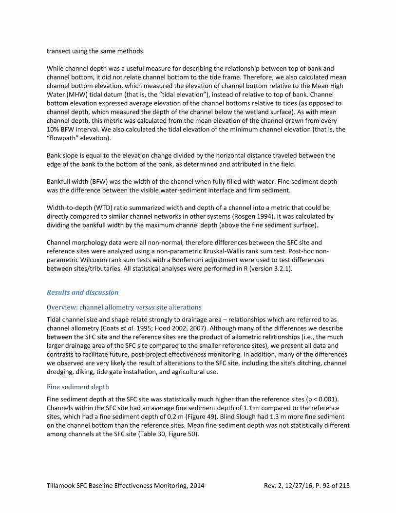
Tillamook SFC Baseline Effectiveness Monitoring, 2014 Rev. 2, 12/27/16, P. 92 of 215
transect using the same methods. While channel depth was a useful measure for describing the relationship between top of bank and channel bottom, it did not relate channel bottom to the tide frame. Therefore, we also calculated mean channel bottom elevation, which measured the elevation of channel bottom relative to the Mean High Water (MHW) tidal datum (that is, the “tidal elevation”), instead of relative to top of bank. Channel bottom elevation expressed average elevation of the channel bottoms relative to tides (as opposed to channel depth, which measured the depth of the channel below the wetland surface). As with mean channel depth, this metric was calculated from the mean elevation of the channel drawn from every 10% BFW interval. We also calculated the tidal elevation of the minimum channel elevation (that is, the “flowpath” elevation). Bank slope is equal to the elevation change divided by the horizontal distance traveled between the edge of the bank to the bottom of the bank, as determined and attributed in the field. Bankfull width (BFW) was the width of the channel when fully filled with water. Fine sediment depth was the difference between the visible water-sediment interface and firm sediment. Width-to-depth (WTD) ratio summarized width and depth of a channel into a metric that could be directly compared to similar channel networks in other systems (Rosgen 1994). It was calculated by dividing the bankfull width by the maximum channel depth (above the fine sediment surface). Channel morphology data were all non-normal, therefore differences between the SFC site and reference sites were analyzed using a non-parametric Kruskal-Wallis rank sum test. Post-hoc non-parametric Wilcoxon rank sum tests with a Bonferroni adjustment were used to test differences between sites/tributaries. All statistical analyses were performed in R (version 3.2.1).
Results and discussion
Overview: channel allometry versus site alterations
Tidal channel size and shape relate strongly to drainage area – relationships which are referred to as channel allometry (Coats et al. 1995; Hood 2002, 2007). Although many of the differences we describe between the SFC site and the reference sites are the product of allometric relationships (i.e., the much larger drainage area of the SFC site compared to the smaller reference sites), we present all data and contrasts to facilitate future, post-project effectiveness monitoring. In addition, many of the differences we observed are very likely the result of alterations to the SFC site, including the site’s ditching, channel dredging, diking, tide gate installation, and agricultural use.
Fine sediment depth
Fine sediment depth at the SFC site was statistically much higher than the reference sites (p < 0.001). Channels within the SFC site had an average fine sediment depth of 1.1 m compared to the reference sites, which had a fine sediment depth of 0.2 m (Figure 49). Blind Slough had 1.3 m more fine sediment on the channel bottom than the reference sites. Mean fine sediment depth was not statistically different among channels at the SFC site (Table 30, Figure 50).
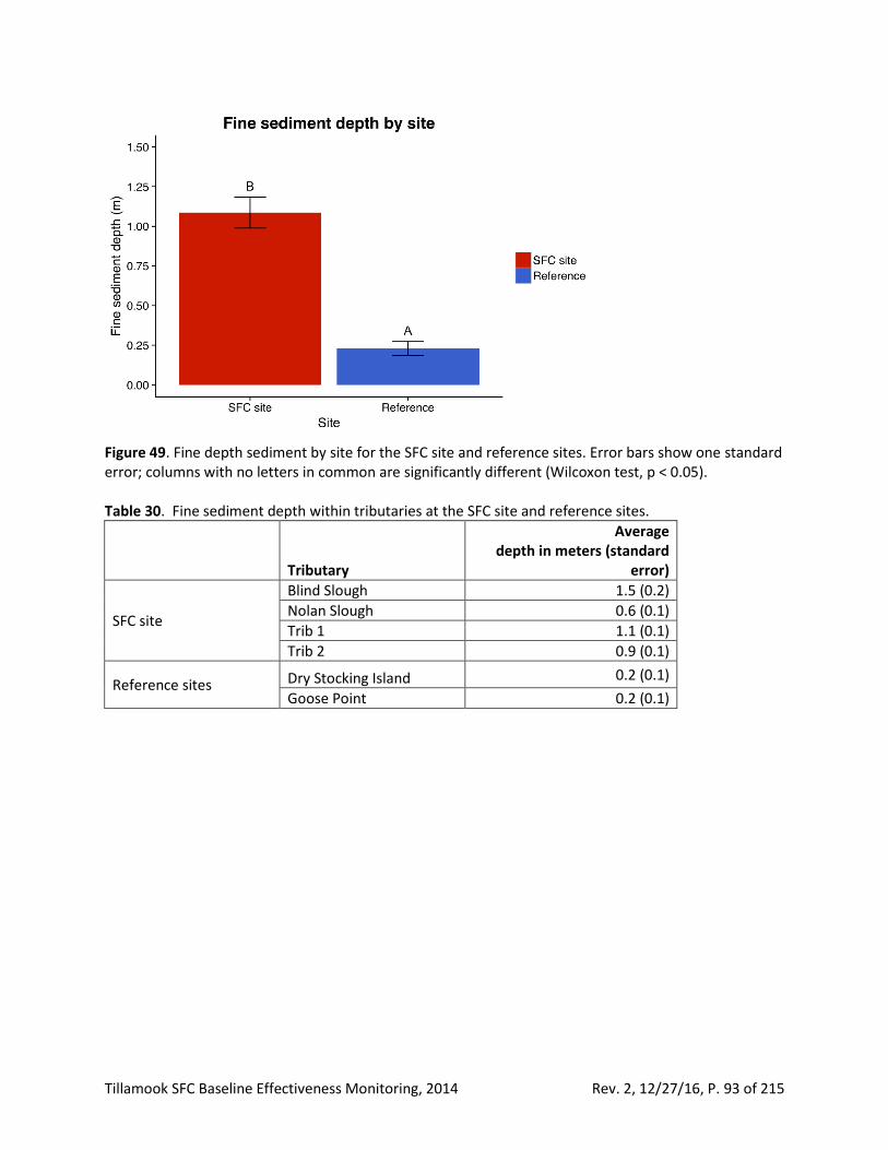
Tillamook SFC Baseline Effectiveness Monitoring, 2014 Rev. 2, 12/27/16, P. 93 of 215
Figure 49. Fine depth sediment by site for the SFC site and reference sites. Error bars show one standard error; columns with no letters in common are significantly different (Wilcoxon test, p < 0.05). Table 30. Fine sediment depth within tributaries at the SFC site and reference sites.
Tributary
Average depth in meters (standard
error)
SFC site
Blind Slough 1.5 (0.2)
Nolan Slough 0.6 (0.1)
Trib 1 1.1 (0.1)
Trib 2 0.9 (0.1)
Reference sites Dry Stocking Island 0.2 (0.1)
Goose Point 0.2 (0.1)
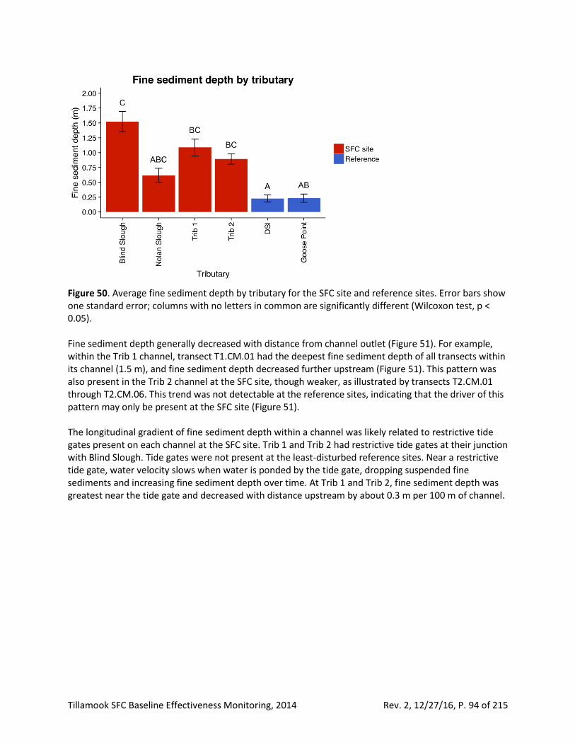
Tillamook SFC Baseline Effectiveness Monitoring, 2014 Rev. 2, 12/27/16, P. 94 of 215
Figure 50. Average fine sediment depth by tributary for the SFC site and reference sites. Error bars show one standard error; columns with no letters in common are significantly different (Wilcoxon test, p < 0.05). Fine sediment depth generally decreased with distance from channel outlet (Figure 51). For example, within the Trib 1 channel, transect T1.CM.01 had the deepest fine sediment depth of all transects within its channel (1.5 m), and fine sediment depth decreased further upstream (Figure 51). This pattern was also present in the Trib 2 channel at the SFC site, though weaker, as illustrated by transects T2.CM.01 through T2.CM.06. This trend was not detectable at the reference sites, indicating that the driver of this pattern may only be present at the SFC site (Figure 51). The longitudinal gradient of fine sediment depth within a channel was likely related to restrictive tide gates present on each channel at the SFC site. Trib 1 and Trib 2 had restrictive tide gates at their junction with Blind Slough. Tide gates were not present at the least-disturbed reference sites. Near a restrictive tide gate, water velocity slows when water is ponded by the tide gate, dropping suspended fine sediments and increasing fine sediment depth over time. At Trib 1 and Trib 2, fine sediment depth was greatest near the tide gate and decreased with distance upstream by about 0.3 m per 100 m of channel.
Tillamook SFC Baseline Effectiveness Monitoring, 2014 Rev. 2, 12/27/16, P. 95 of 215
Figure 51. Fine sediment depth by transect for the SFC site and reference sites. Error bars represent one standard error. Bars of the same color represent transects within the same channel. The Blind Slough channel at the SFC site also illustrated the relationship between the presence of a restrictive tide gate and fine sediment depth. Channel morphology transects BS.CM.01 through BS.CM.04 were below major tide gates on the Blind Slough channel, while BS.CM.05 through BS.CM.09 were above the tide gate (Map A15). On Blind Slough, fine sediment depth was lowest (0.8 m – 1.0 m) near the mouth of the channel (BS.CM.01), where there was full tidal exchange with Tillamook Bay on every tide cycle. Fine sediment depth dramatically increased to approximately 1.8 m at the BS.CM.03 transect (Figure 51). Fine sediment depth remained high at transects BS.CM.05 through BS.CM.07, immediately upstream of the restrictive tide gates on Blind Slough. While Blind Slough transects BS.CM.08 and BS.CM.09 had the highest fine sediment depth of all transects within the Blind Slough channel, they measured two ponded areas that were not representative of the rest of the Blind Slough channel. Overall, the much greater depth of fine sediment at the SFC site compared to the reference sites was likely related to the site’s land use history and tidal restrictions. Fine sediments typically accumulate in ditches of diked pastures, requiring repeated ditch maintenance. Sediment accumulation is likely due to reduced flow velocities and channel bank degradation by livestock, as well as accumulation of organic matter from aquatic vegetation. We observed massive mats of aquatic vegetation in many channels at the SFC site; parrotfeather milfoil (Millefolium aquaticum) was particularly abundant and dense. This abundant aquatic vegetation reflects the relatively stable water levels inside the site, compared to the water level fluctuations that would occur if tidal barriers (dikes and tide gates) were not in place. The more stable water levels are reflected in the relatively consistent elevation and low gradient of the fine sediment surface, compared to the steeper and more variable firm channel bottom surface (Figure 61). Following implementation of the SFC project, we expect fine sediment depth to decrease within the SFC site, eventually resembling depths found at the reference sites. This process may take many years following tidal reconnection, as sediment within the SFC site is remobilized and transported within the site before being exported. We observed a similar process at the Ni-les’tun restoration project of the
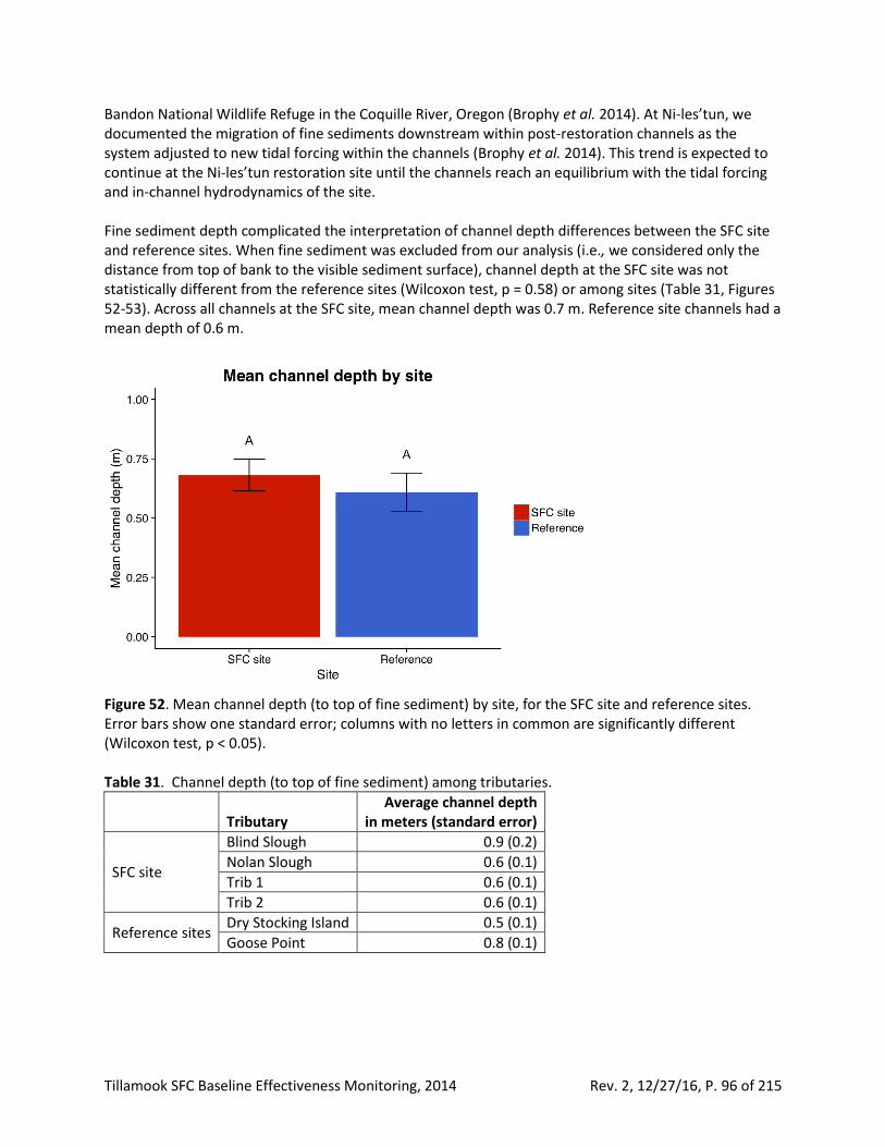
Tillamook SFC Baseline Effectiveness Monitoring, 2014 Rev. 2, 12/27/16, P. 96 of 215
Bandon National Wildlife Refuge in the Coquille River, Oregon (Brophy et al. 2014). At Ni-les’tun, we documented the migration of fine sediments downstream within post-restoration channels as the system adjusted to new tidal forcing within the channels (Brophy et al. 2014). This trend is expected to continue at the Ni-les’tun restoration site until the channels reach an equilibrium with the tidal forcing and in-channel hydrodynamics of the site. Fine sediment depth complicated the interpretation of channel depth differences between the SFC site and reference sites. When fine sediment was excluded from our analysis (i.e., we considered only the distance from top of bank to the visible sediment surface), channel depth at the SFC site was not statistically different from the reference sites (Wilcoxon test, p = 0.58) or among sites (Table 31, Figures 52-53). Across all channels at the SFC site, mean channel depth was 0.7 m. Reference site channels had a mean depth of 0.6 m.
Figure 52. Mean channel depth (to top of fine sediment) by site, for the SFC site and reference sites. Error bars show one standard error; columns with no letters in common are significantly different (Wilcoxon test, p < 0.05). Table 31. Channel depth (to top of fine sediment) among tributaries.
Tributary
Average channel depth in meters (standard error)
SFC site
Blind Slough 0.9 (0.2)
Nolan Slough 0.6 (0.1)
Trib 1 0.6 (0.1)
Trib 2 0.6 (0.1)
Reference sites Dry Stocking Island 0.5 (0.1)
Goose Point 0.8 (0.1)
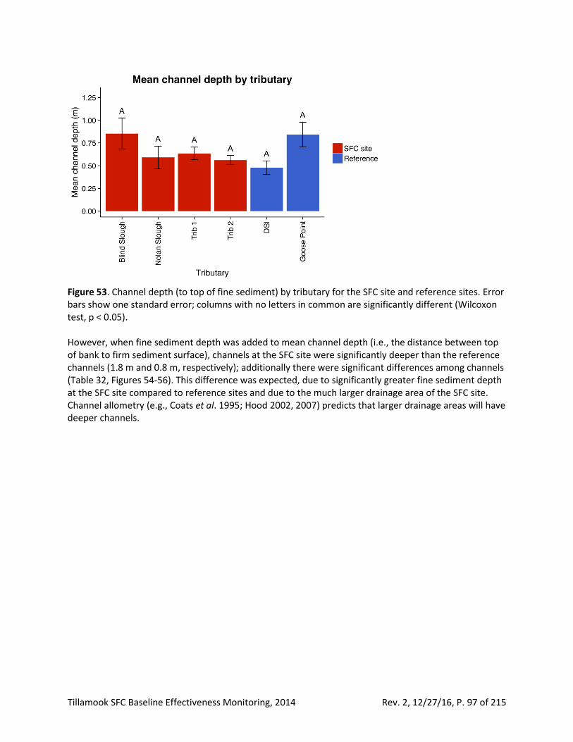
Tillamook SFC Baseline Effectiveness Monitoring, 2014 Rev. 2, 12/27/16, P. 97 of 215
Figure 53. Channel depth (to top of fine sediment) by tributary for the SFC site and reference sites. Error bars show one standard error; columns with no letters in common are significantly different (Wilcoxon test, p < 0.05). However, when fine sediment depth was added to mean channel depth (i.e., the distance between top of bank to firm sediment surface), channels at the SFC site were significantly deeper than the reference channels (1.8 m and 0.8 m, respectively); additionally there were significant differences among channels (Table 32, Figures 54-56). This difference was expected, due to significantly greater fine sediment depth at the SFC site compared to reference sites and due to the much larger drainage area of the SFC site. Channel allometry (e.g., Coats et al. 1995; Hood 2002, 2007) predicts that larger drainage areas will have deeper channels.
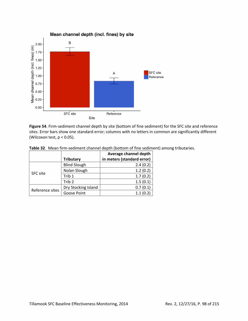
Tillamook SFC Baseline Effectiveness Monitoring, 2014 Rev. 2, 12/27/16, P. 98 of 215
Figure 54. Firm-sediment channel depth by site (bottom of fine sediment) for the SFC site and reference sites. Error bars show one standard error; columns with no letters in common are significantly different (Wilcoxon test, p < 0.05). Table 32. Mean firm-sediment channel depth (bottom of fine sediment) among tributaries.
Tributary
Average channel depth in meters (standard error)
SFC site
Blind Slough 2.4 (0.2)
Nolan Slough 1.2 (0.2)
Trib 1 1.7 (0.2)
Trib 2 1.5 (0.1)
Reference sites Dry Stocking Island 0.7 (0.1)
Goose Point 1.1 (0.2)
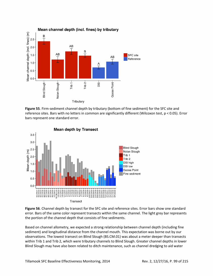
Tillamook SFC Baseline Effectiveness Monitoring, 2014 Rev. 2, 12/27/16, P. 99 of 215
Figure 55. Firm-sediment channel depth by tributary (bottom of fine sediment) for the SFC site and reference sites. Bars with no letters in common are significantly different (Wilcoxon test, p < 0.05). Error bars represent one standard error.
Figure 56. Channel depth by transect for the SFC site and reference sites. Error bars show one standard error. Bars of the same color represent transects within the same channel. The light grey bar represents the portion of the channel depth that consists of fine sediments. Based on channel allometry, we expected a strong relationship between channel depth (including fine sediment) and longitudinal distance from the channel mouth. This expectation was borne out by our observations. The lowest transect on Blind Slough (BS.CM.01) was about a meter deeper than transects within Trib 1 and Trib 2, which were tributary channels to Blind Slough. Greater channel depths in lower Blind Slough may have also been related to ditch maintenance, such as channel dredging to aid water
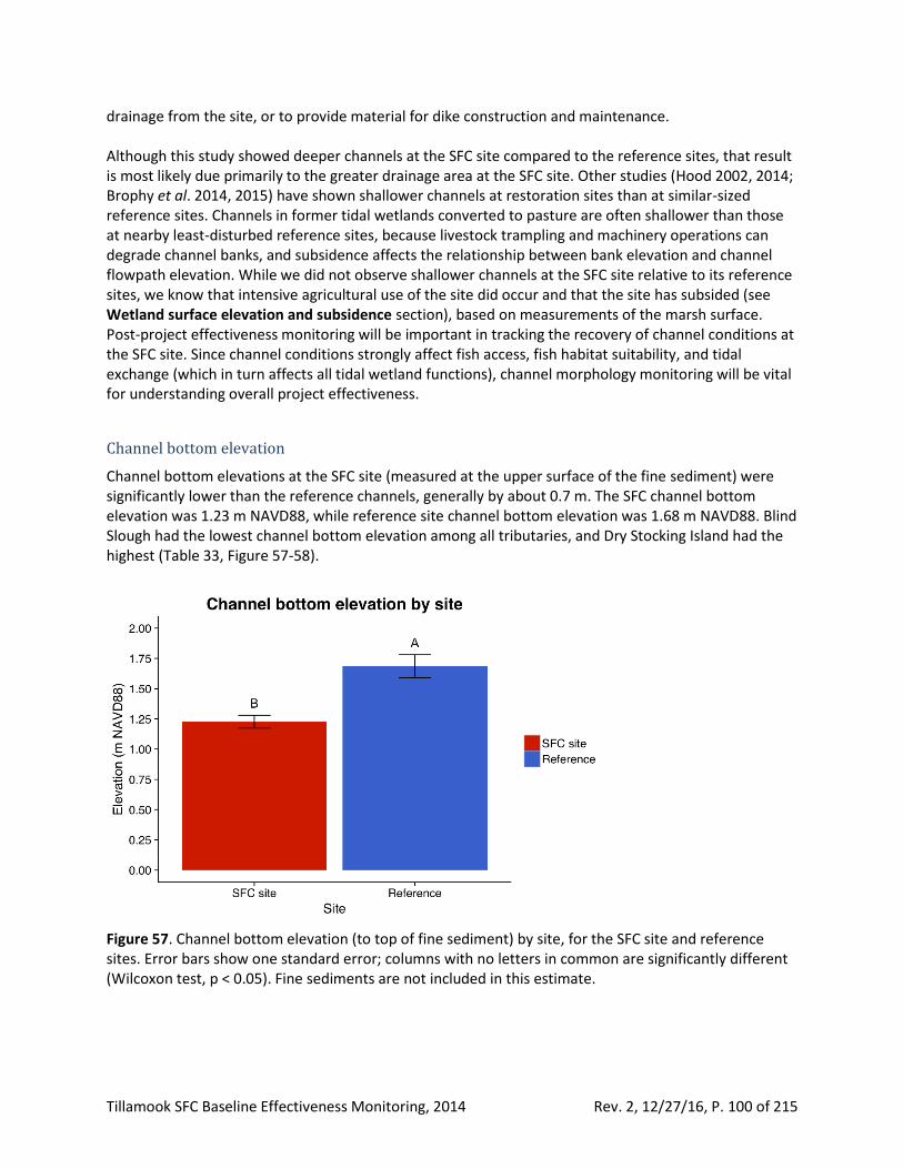
Tillamook SFC Baseline Effectiveness Monitoring, 2014 Rev. 2, 12/27/16, P. 100 of 215
drainage from the site, or to provide material for dike construction and maintenance. Although this study showed deeper channels at the SFC site compared to the reference sites, that result is most likely due primarily to the greater drainage area at the SFC site. Other studies (Hood 2002, 2014; Brophy et al. 2014, 2015) have shown shallower channels at restoration sites than at similar-sized reference sites. Channels in former tidal wetlands converted to pasture are often shallower than those at nearby least-disturbed reference sites, because livestock trampling and machinery operations can degrade channel banks, and subsidence affects the relationship between bank elevation and channel flowpath elevation. While we did not observe shallower channels at the SFC site relative to its reference sites, we know that intensive agricultural use of the site did occur and that the site has subsided (see Wetland surface elevation and subsidence section), based on measurements of the marsh surface. Post-project effectiveness monitoring will be important in tracking the recovery of channel conditions at the SFC site. Since channel conditions strongly affect fish access, fish habitat suitability, and tidal exchange (which in turn affects all tidal wetland functions), channel morphology monitoring will be vital for understanding overall project effectiveness.
Channel bottom elevation
Channel bottom elevations at the SFC site (measured at the upper surface of the fine sediment) were significantly lower than the reference channels, generally by about 0.7 m. The SFC channel bottom elevation was 1.23 m NAVD88, while reference site channel bottom elevation was 1.68 m NAVD88. Blind Slough had the lowest channel bottom elevation among all tributaries, and Dry Stocking Island had the highest (Table 33, Figure 57-58).
Figure 57. Channel bottom elevation (to top of fine sediment) by site, for the SFC site and reference sites. Error bars show one standard error; columns with no letters in common are significantly different (Wilcoxon test, p < 0.05). Fine sediments are not included in this estimate.
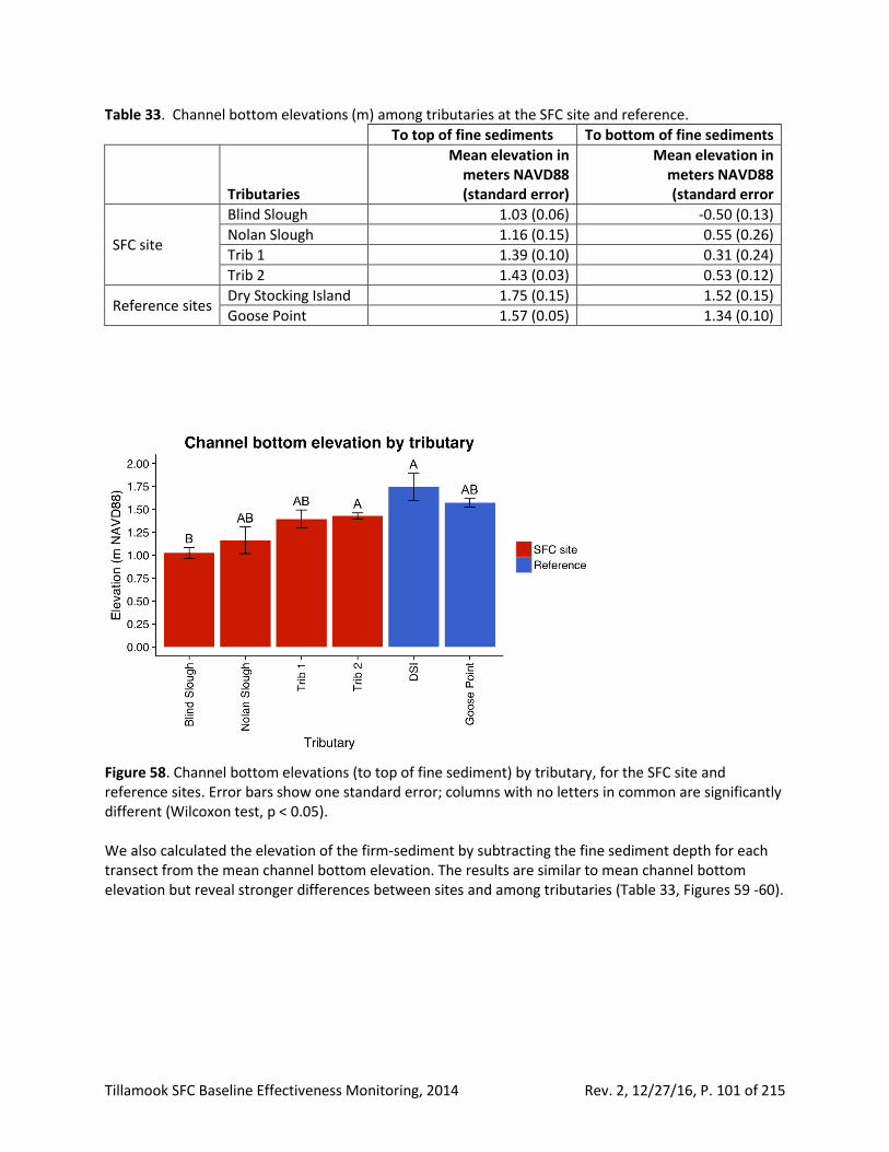
Tillamook SFC Baseline Effectiveness Monitoring, 2014 Rev. 2, 12/27/16, P. 101 of 215
Table 33. Channel bottom elevations (m) among tributaries at the SFC site and reference.
To top of fine sediments To bottom of fine sediments
Tributaries
Mean elevation in meters NAVD88 (standard error)
Mean elevation in meters NAVD88 (standard error
SFC site
Blind Slough 1.03 (0.06) -0.50 (0.13)
Nolan Slough 1.16 (0.15) 0.55 (0.26)
Trib 1 1.39 (0.10) 0.31 (0.24)
Trib 2 1.43 (0.03) 0.53 (0.12)
Reference sites Dry Stocking Island 1.75 (0.15) 1.52 (0.15)
Goose Point 1.57 (0.05) 1.34 (0.10)
Figure 58. Channel bottom elevations (to top of fine sediment) by tributary, for the SFC site and reference sites. Error bars show one standard error; columns with no letters in common are significantly different (Wilcoxon test, p < 0.05). We also calculated the elevation of the firm-sediment by subtracting the fine sediment depth for each transect from the mean channel bottom elevation. The results are similar to mean channel bottom elevation but reveal stronger differences between sites and among tributaries (Table 33, Figures 59 -60).
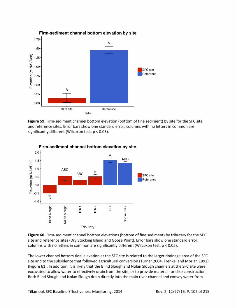
Tillamook SFC Baseline Effectiveness Monitoring, 2014 Rev. 2, 12/27/16, P. 102 of 215
Figure 59. Firm-sediment channel bottom elevation (bottom of fine sediment) by site for the SFC site and reference sites. Error bars show one standard error; columns with no letters in common are significantly different (Wilcoxon test, p < 0.05).
Figure 60. Firm-sediment channel bottom elevations (bottom of fine sediment) by tributary for the SFC site and reference sites (Dry Stocking Island and Goose Point). Error bars show one standard error; columns with no letters in common are significantly different (Wilcoxon test, p < 0.05). The lower channel bottom tidal elevation at the SFC site is related to the larger drainage area of the SFC site and to the subsidence that followed agricultural conversion (Turner 2004, Frenkel and Morlan 1991) (Figure 61). In addition, it is likely that the Blind Slough and Nolan Slough channels at the SFC site were excavated to allow water to effectively drain from the site, or to provide material for dike construction. Both Blind Slough and Nolan Slough drain directly into the main river channel and convey water from
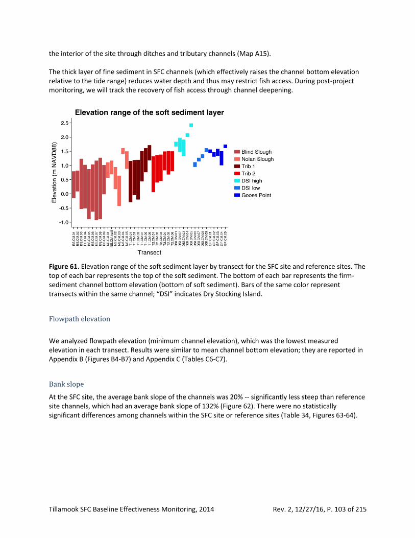
Tillamook SFC Baseline Effectiveness Monitoring, 2014 Rev. 2, 12/27/16, P. 103 of 215
the interior of the site through ditches and tributary channels (Map A15). The thick layer of fine sediment in SFC channels (which effectively raises the channel bottom elevation relative to the tide range) reduces water depth and thus may restrict fish access. During post-project monitoring, we will track the recovery of fish access through channel deepening.
Figure 61. Elevation range of the soft sediment layer by transect for the SFC site and reference sites. The top of each bar represents the top of the soft sediment. The bottom of each bar represents the firm-sediment channel bottom elevation (bottom of soft sediment). Bars of the same color represent transects within the same channel; “DSI” indicates Dry Stocking Island.
Flowpath elevation
We analyzed flowpath elevation (minimum channel elevation), which was the lowest measured elevation in each transect. Results were similar to mean channel bottom elevation; they are reported in Appendix B (Figures B4-B7) and Appendix C (Tables C6-C7).
Bank slope
At the SFC site, the average bank slope of the channels was 20% -- significantly less steep than reference site channels, which had an average bank slope of 132% (Figure 62). There were no statistically significant differences among channels within the SFC site or reference sites (Table 34, Figures 63-64).
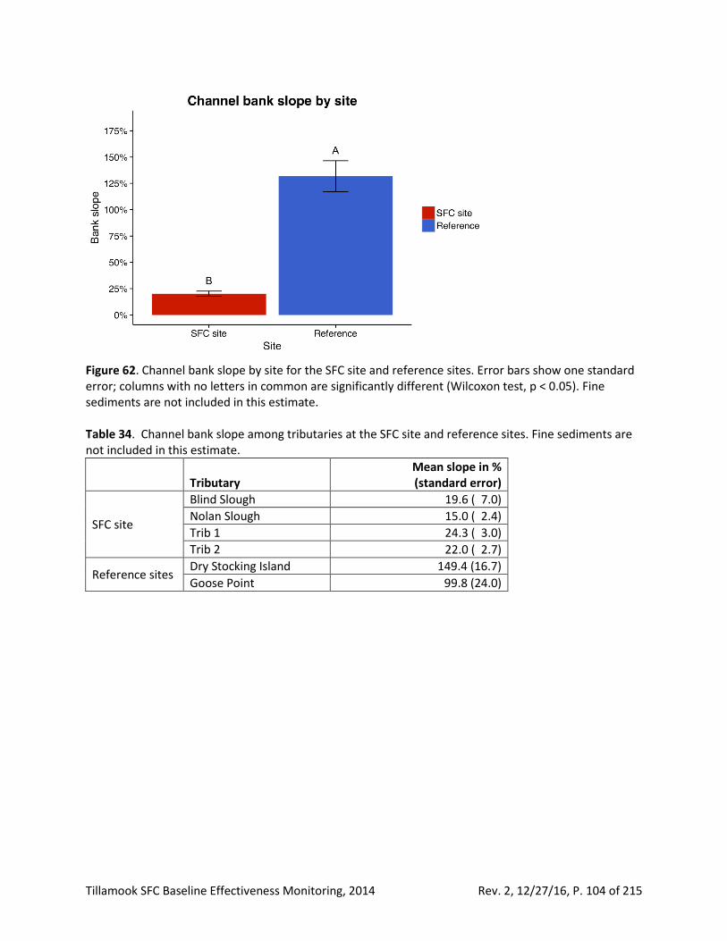
Tillamook SFC Baseline Effectiveness Monitoring, 2014 Rev. 2, 12/27/16, P. 104 of 215
Figure 62. Channel bank slope by site for the SFC site and reference sites. Error bars show one standard error; columns with no letters in common are significantly different (Wilcoxon test, p < 0.05). Fine sediments are not included in this estimate. Table 34. Channel bank slope among tributaries at the SFC site and reference sites. Fine sediments are not included in this estimate.
Tributary Mean slope in % (standard error)
SFC site
Blind Slough 19.6 ( 7.0)
Nolan Slough 15.0 ( 2.4)
Trib 1 24.3 ( 3.0)
Trib 2 22.0 ( 2.7)
Reference sites Dry Stocking Island 149.4 (16.7)
Goose Point 99.8 (24.0)
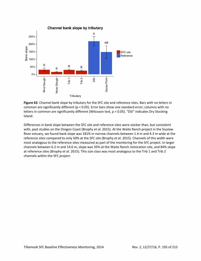
Tillamook SFC Baseline Effectiveness Monitoring, 2014 Rev. 2, 12/27/16, P. 105 of 215
Figure 63. Channel bank slope by tributary for the SFC site and reference sites. Bars with no letters in common are significantly different (p < 0.05). Error bars show one standard error; columns with no letters in common are significantly different (Wilcoxon test, p < 0.05). “DSI” indicates Dry Stocking Island. Differences in bank slope between the SFC site and reference sites were starker than, but consistent with, past studies on the Oregon Coast (Brophy et al. 2015). At the Waite Ranch project in the Siuslaw River estuary, we found bank slope was 181% in narrow channels between 1.4 m and 4.3 m wide at the reference sites compared to only 50% at the SFC site (Brophy et al. 2015). Channels of this width were most analogous to the reference sites measured as part of the monitoring for the SFC project. In larger channels between 6.2 m and 14.6 m, slope was 35% at the Waite Ranch restoration site, and 84% slope at reference sites (Brophy et al. 2015). This size class was most analogous to the Trib 1 and Trib 2 channels within the SFC project.
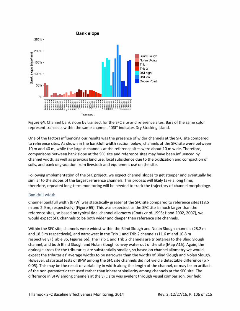
Tillamook SFC Baseline Effectiveness Monitoring, 2014 Rev. 2, 12/27/16, P. 106 of 215
Figure 64. Channel bank slope by transect for the SFC site and reference sites. Bars of the same color represent transects within the same channel. “DSI” indicates Dry Stocking Island. One of the factors influencing our results was the presence of wider channels at the SFC site compared to reference sites. As shown in the bankfull width section below, channels at the SFC site were between 10 m and 40 m, while the largest channels at the reference sites were about 10 m wide. Therefore, comparisons between bank slope at the SFC site and reference sites may have been influenced by channel width, as well as previous land use, local subsidence due to the oxidization and compaction of soils, and bank degradation from livestock and equipment use on the site. Following implementation of the SFC project, we expect channel slopes to get steeper and eventually be similar to the slopes of the largest reference channels. This process will likely take a long time; therefore, repeated long-term monitoring will be needed to track the trajectory of channel morphology.
Bankfull width
Channel bankfull width (BFW) was statistically greater at the SFC site compared to reference sites (18.5 m and 2.9 m, respectively) (Figure 65). This was expected, as the SFC site is much larger than the reference sites, so based on typical tidal channel allometry (Coats et al. 1995; Hood 2002, 2007), we would expect SFC channels to be both wider and deeper than reference site channels. Within the SFC site, channels were widest within the Blind Slough and Nolan Slough channels (28.2 m and 18.5 m respectively), and narrowest in the Trib 1 and Trib 2 channels (11.6 m and 10.8 m respectively) (Table 35, Figures 66). The Trib 1 and Trib 2 channels are tributaries to the Blind Slough channel, and both Blind Slough and Nolan Slough convey water out of the site (Map A15). Again, the drainage areas for the tributaries are substantially smaller, so based on channel allometry we would expect the tributaries’ average widths to be narrower than the widths of Blind Slough and Nolan Slough. However, statistical tests of BFW among the SFC site channels did not yield a detectable difference (p > 0.05). This may be the result of variability in width along the length of the channel, or may be an artifact of the non-parametric test used rather than inherent similarity among channels at the SFC site. The difference in BFW among channels at the SFC site was evident through visual comparison, our field
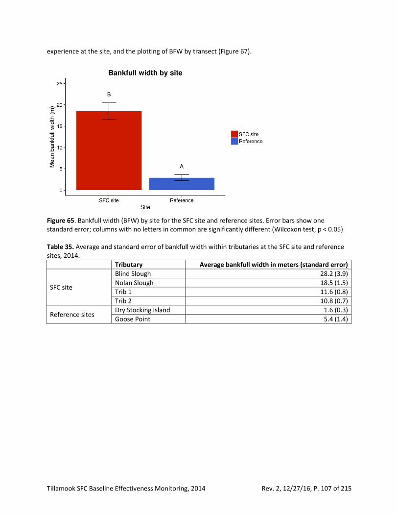
Tillamook SFC Baseline Effectiveness Monitoring, 2014 Rev. 2, 12/27/16, P. 107 of 215
experience at the site, and the plotting of BFW by transect (Figure 67).
Figure 65. Bankfull width (BFW) by site for the SFC site and reference sites. Error bars show one standard error; columns with no letters in common are significantly different (Wilcoxon test, p < 0.05). Table 35. Average and standard error of bankfull width within tributaries at the SFC site and reference sites, 2014.
Tributary Average bankfull width in meters (standard error)
SFC site
Blind Slough 28.2 (3.9)
Nolan Slough 18.5 (1.5)
Trib 1 11.6 (0.8)
Trib 2 10.8 (0.7)
Reference sites Dry Stocking Island 1.6 (0.3)
Goose Point 5.4 (1.4)
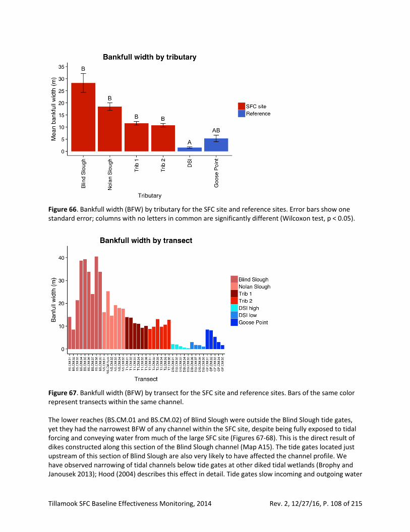
Tillamook SFC Baseline Effectiveness Monitoring, 2014 Rev. 2, 12/27/16, P. 108 of 215
Figure 66. Bankfull width (BFW) by tributary for the SFC site and reference sites. Error bars show one standard error; columns with no letters in common are significantly different (Wilcoxon test, p < 0.05).
Figure 67. Bankfull width (BFW) by transect for the SFC site and reference sites. Bars of the same color represent transects within the same channel. The lower reaches (BS.CM.01 and BS.CM.02) of Blind Slough were outside the Blind Slough tide gates, yet they had the narrowest BFW of any channel within the SFC site, despite being fully exposed to tidal forcing and conveying water from much of the large SFC site (Figures 67-68). This is the direct result of dikes constructed along this section of the Blind Slough channel (Map A15). The tide gates located just upstream of this section of Blind Slough are also very likely to have affected the channel profile. We have observed narrowing of tidal channels below tide gates at other diked tidal wetlands (Brophy and Janousek 2013); Hood (2004) describes this effect in detail. Tide gates slow incoming and outgoing water
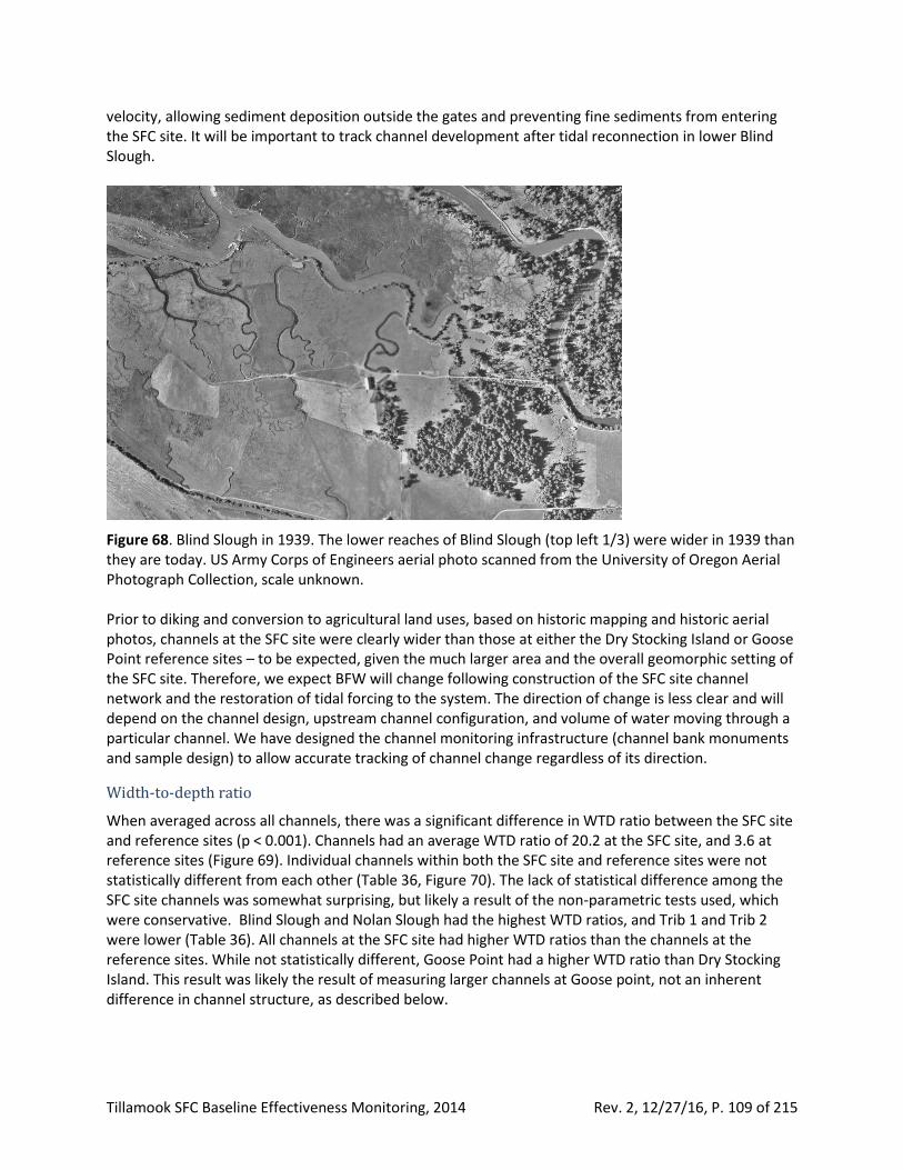
Tillamook SFC Baseline Effectiveness Monitoring, 2014 Rev. 2, 12/27/16, P. 109 of 215
velocity, allowing sediment deposition outside the gates and preventing fine sediments from entering the SFC site. It will be important to track channel development after tidal reconnection in lower Blind Slough.
Figure 68. Blind Slough in 1939. The lower reaches of Blind Slough (top left 1/3) were wider in 1939 than they are today. US Army Corps of Engineers aerial photo scanned from the University of Oregon Aerial Photograph Collection, scale unknown. Prior to diking and conversion to agricultural land uses, based on historic mapping and historic aerial photos, channels at the SFC site were clearly wider than those at either the Dry Stocking Island or Goose Point reference sites – to be expected, given the much larger area and the overall geomorphic setting of the SFC site. Therefore, we expect BFW will change following construction of the SFC site channel network and the restoration of tidal forcing to the system. The direction of change is less clear and will depend on the channel design, upstream channel configuration, and volume of water moving through a particular channel. We have designed the channel monitoring infrastructure (channel bank monuments and sample design) to allow accurate tracking of channel change regardless of its direction.
Width-to-depth ratio
When averaged across all channels, there was a significant difference in WTD ratio between the SFC site and reference sites (p < 0.001). Channels had an average WTD ratio of 20.2 at the SFC site, and 3.6 at reference sites (Figure 69). Individual channels within both the SFC site and reference sites were not statistically different from each other (Table 36, Figure 70). The lack of statistical difference among the SFC site channels was somewhat surprising, but likely a result of the non-parametric tests used, which were conservative. Blind Slough and Nolan Slough had the highest WTD ratios, and Trib 1 and Trib 2 were lower (Table 36). All channels at the SFC site had higher WTD ratios than the channels at the reference sites. While not statistically different, Goose Point had a higher WTD ratio than Dry Stocking Island. This result was likely the result of measuring larger channels at Goose point, not an inherent difference in channel structure, as described below.
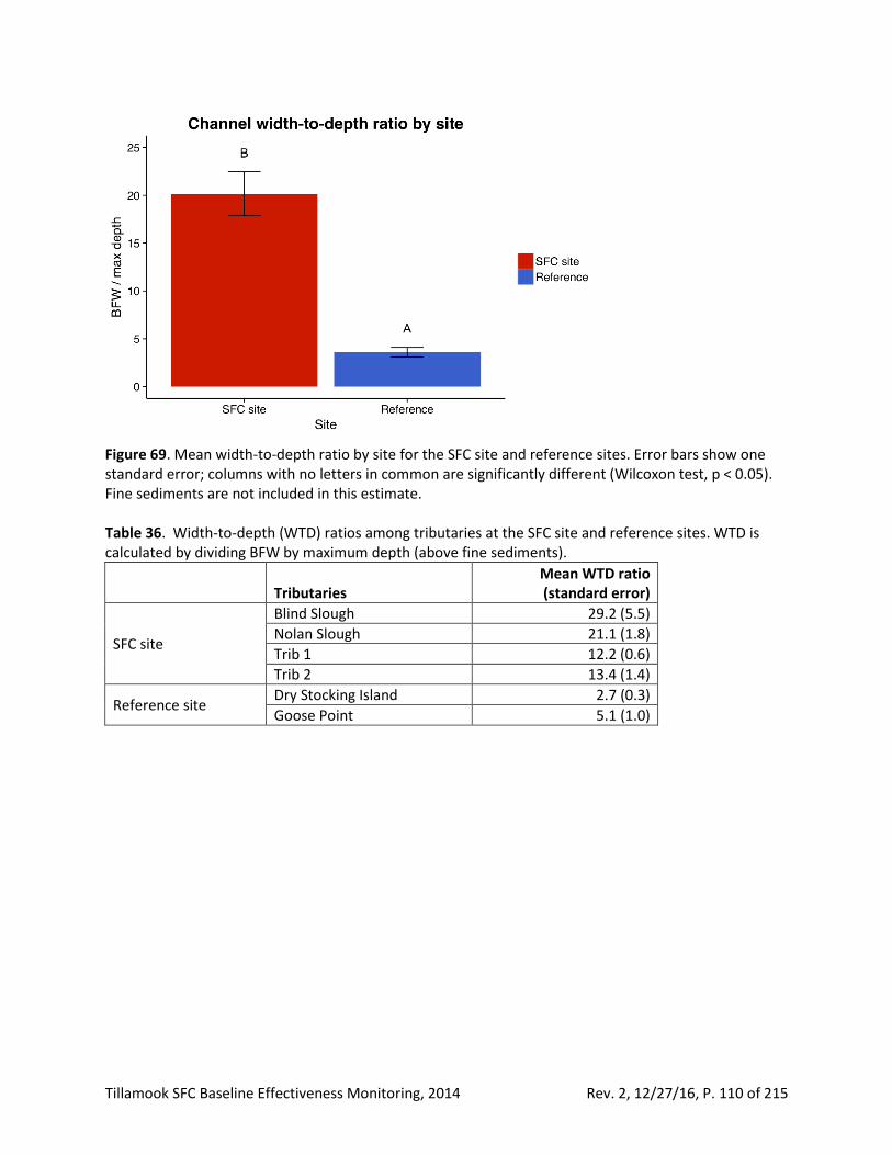
Tillamook SFC Baseline Effectiveness Monitoring, 2014 Rev. 2, 12/27/16, P. 110 of 215
Figure 69. Mean width-to-depth ratio by site for the SFC site and reference sites. Error bars show one standard error; columns with no letters in common are significantly different (Wilcoxon test, p < 0.05). Fine sediments are not included in this estimate. Table 36. Width-to-depth (WTD) ratios among tributaries at the SFC site and reference sites. WTD is calculated by dividing BFW by maximum depth (above fine sediments).
Tributaries Mean WTD ratio (standard error)
SFC site
Blind Slough 29.2 (5.5)
Nolan Slough 21.1 (1.8)
Trib 1 12.2 (0.6)
Trib 2 13.4 (1.4)
Reference site Dry Stocking Island 2.7 (0.3)
Goose Point 5.1 (1.0)
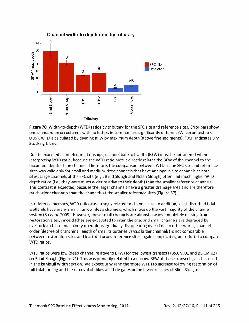
Tillamook SFC Baseline Effectiveness Monitoring, 2014 Rev. 2, 12/27/16, P. 111 of 215
Figure 70. Width-to-depth (WTD) ratios by tributary for the SFC site and reference sites. Error bars show one standard error; columns with no letters in common are significantly different (Wilcoxon test, p < 0.05). WTD is calculated by dividing BFW by maximum depth (above fine sediments). “DSI” indicates Dry Stocking Island. Due to expected allometric relationships, channel bankfull width (BFW) must be considered when interpreting WTD ratio, because the WTD ratio metric directly relates the BFW of the channel to the maximum depth of the channel. Therefore, the comparison between WTD at the SFC site and reference sites was valid only for small and medium-sized channels that have analogous size channels at both sites. Large channels at the SFC site (e.g., Blind Slough and Nolan Slough) often had much higher WTD depth ratios (i.e., they were much wider relative to their depth) than the smaller reference channels. This contrast is expected, because the larger channels have a greater drainage area and are therefore much wider channels than the channels at the smaller reference sites (Figure 67). In reference marshes, WTD ratio was strongly related to channel size. In addition, least-disturbed tidal wetlands have many small, narrow, deep channels, which make up the vast majority of the channel system (So et al. 2009). However, these small channels are almost always completely missing from restoration sites, since ditches are excavated to drain the site, and small channels are degraded by livestock and farm machinery operations, gradually disappearing over time. In other words, channel order (degree of branching, length of small tributaries versus larger channels) is not comparable between restoration sites and least-disturbed reference sites; again complicating our efforts to compare WTD ratios. WTD ratios were low (deep channel relative to BFW) for the lowest transects (BS.CM.01 and BS.CM.02) on Blind Slough (Figure 71). This was primarily related to a narrow BFW at these transects, as discussed in the bankfull width section. We expect BFW (and therefore WTD) to increase following restoration of full tidal forcing and the removal of dikes and tide gates in the lower reaches of Blind Slough.
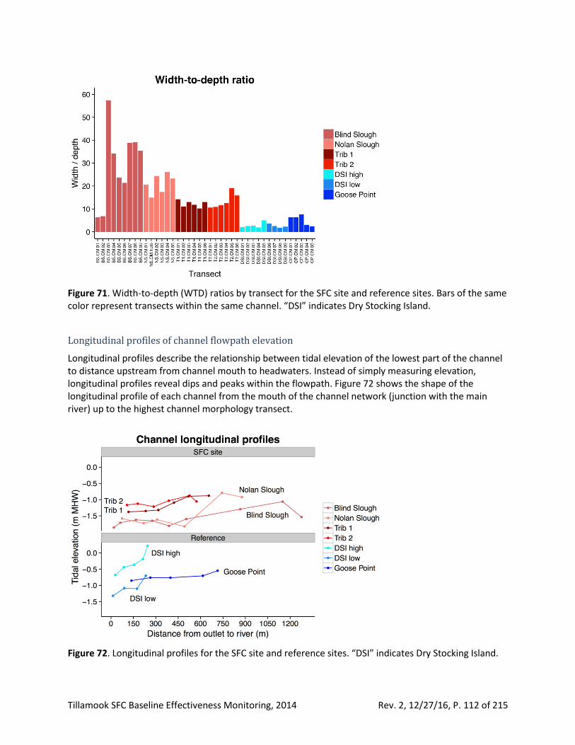
Tillamook SFC Baseline Effectiveness Monitoring, 2014 Rev. 2, 12/27/16, P. 112 of 215
Figure 71. Width-to-depth (WTD) ratios by transect for the SFC site and reference sites. Bars of the same color represent transects within the same channel. “DSI” indicates Dry Stocking Island.
Longitudinal profiles of channel flowpath elevation
Longitudinal profiles describe the relationship between tidal elevation of the lowest part of the channel to distance upstream from channel mouth to headwaters. Instead of simply measuring elevation, longitudinal profiles reveal dips and peaks within the flowpath. Figure 72 shows the shape of the longitudinal profile of each channel from the mouth of the channel network (junction with the main river) up to the highest channel morphology transect.
Figure 72. Longitudinal profiles for the SFC site and reference sites. “DSI” indicates Dry Stocking Island.
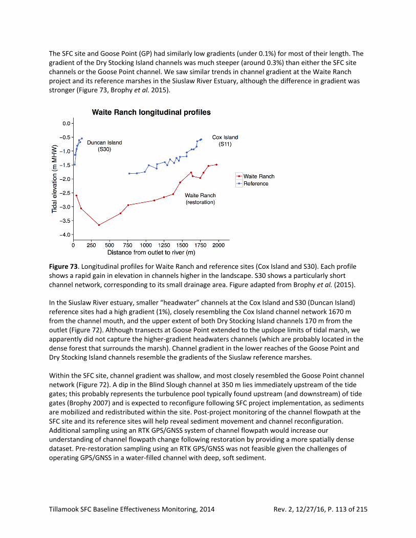
Tillamook SFC Baseline Effectiveness Monitoring, 2014 Rev. 2, 12/27/16, P. 113 of 215
The SFC site and Goose Point (GP) had similarly low gradients (under 0.1%) for most of their length. The gradient of the Dry Stocking Island channels was much steeper (around 0.3%) than either the SFC site channels or the Goose Point channel. We saw similar trends in channel gradient at the Waite Ranch project and its reference marshes in the Siuslaw River Estuary, although the difference in gradient was stronger (Figure 73, Brophy et al. 2015).
Figure 73. Longitudinal profiles for Waite Ranch and reference sites (Cox Island and S30). Each profile shows a rapid gain in elevation in channels higher in the landscape. S30 shows a particularly short channel network, corresponding to its small drainage area. Figure adapted from Brophy et al. (2015). In the Siuslaw River estuary, smaller “headwater” channels at the Cox Island and S30 (Duncan Island) reference sites had a high gradient (1%), closely resembling the Cox Island channel network 1670 m from the channel mouth, and the upper extent of both Dry Stocking Island channels 170 m from the outlet (Figure 72). Although transects at Goose Point extended to the upslope limits of tidal marsh, we apparently did not capture the higher-gradient headwaters channels (which are probably located in the dense forest that surrounds the marsh). Channel gradient in the lower reaches of the Goose Point and Dry Stocking Island channels resemble the gradients of the Siuslaw reference marshes. Within the SFC site, channel gradient was shallow, and most closely resembled the Goose Point channel network (Figure 72). A dip in the Blind Slough channel at 350 m lies immediately upstream of the tide gates; this probably represents the turbulence pool typically found upstream (and downstream) of tide gates (Brophy 2007) and is expected to reconfigure following SFC project implementation, as sediments are mobilized and redistributed within the site. Post-project monitoring of the channel flowpath at the SFC site and its reference sites will help reveal sediment movement and channel reconfiguration. Additional sampling using an RTK GPS/GNSS system of channel flowpath would increase our understanding of channel flowpath change following restoration by providing a more spatially dense dataset. Pre-restoration sampling using an RTK GPS/GNSS was not feasible given the challenges of operating GPS/GNSS in a water-filled channel with deep, soft sediment.

Tillamook SFC Baseline Effectiveness Monitoring, 2014 Rev. 2, 12/27/16, P. 114 of 215
Summary
Our results fit with expectations for the diked, ditched, and hydrologically-altered context of the SFC site, and considering the much larger size of the SFC site compared to the reference sites. The main channels at the SFC site (Blind Slough and Nolan Slough) are deep compared to reference channels and may have been dredged (excavated) to aid water flow out of the site on outgoing tides. Channels were deeper (relative to top of bank) and lower in elevation than the reference channels when fine sediments were included in the analysis. Across all channels at the SFC site, bank slope was significantly less, and width-to-depth ratios were significant greater than at the reference sites (Figure 62 and Figure 69). Monitoring channel morphology at representative locations along the full length of the channel system is important to understanding channel recovery; and flowpath measurements along the longitudinal profile revealed a break in channel gradient near the upper end of each channel -- a pattern that has been observed in other estuaries on the Oregon Coast. As tidal forces are reintroduced to the SFC site following construction of the project, we expect to see channel morphology shift towards equilibrium with those tidal flows, providing an increasingly high quality and quantity of fish habitat, and ultimately resembling reference site channel morphology (for similar-sized drainage areas). In post-construction monitoring, measurements of transect-level changes and statistical summaries of those changes will yield more precise insight into the effect of project construction and the readjustment of the channels at the SFC site through time at the transect, channel, and tributary spatial scales. Repeated time-series monitoring will be critical to identifying the trajectory of change within the site.
Sediment accretion and erosion During the 2014 baseline monitoring period, sediment accretion sample stations were established, and baseline accretion rates were monitored at the SFC site and reference sites. The baseline accretion rates will be compared to post-project monitoring data accretion rates to help determine the project’s effects. Sediment accretion has cascading effects on plant community establishment, habitat development, and climate change resilience. As stated in Brophy and van de Wetering (2014), determining these rates will help us:
• Quantify changes in vertical accretion or erosion after project implementation;
• Determine whether accretion rates in wetlands in the project site are comparable to, or exceed, projected rates of sea level rise; and
• Help interpret the results of other monitored parameters including plant communities, fish populations, and water quality (i.e., turbidity), which will help define relationships between sedimentation and the post-implementation trajectory for these and other parameters.
Methods Baseline monitoring of sediment accretion at the SFC site and nearby reference marshes used two methods: feldspar marker horizon plots combined with cryocore sampling (Cahoon and Turner 1989, Cahoon et al. 2006), and the sediment stake method (Roegner et al. 2008). Feldspar plots and sediment stakes were installed adjacent to each other to allow for direct comparison between the two methods. A total of 38 plots were established using a stratified random sample design, as described in General sample design above. All sediment accretion plots were marked with a 3 m PVC marker pole to help prevent disturbance during farming or project implementation.

Tillamook SFC Baseline Effectiveness Monitoring, 2014 Rev. 2, 12/27/16, P. 115 of 215
All plots and sediment stakes were installed in the fall of 2013 and sampled after one year (November 2014), yielding a baseline accretion rate per year. The location and elevation of each plot was recorded in October 2013 using a high-precision RTK GPS/GNSS system (Table 37). Plot A69 at Goose Point was removed as an outlier from all feldspar related analyses, since an error occurred during field sampling at that plot.
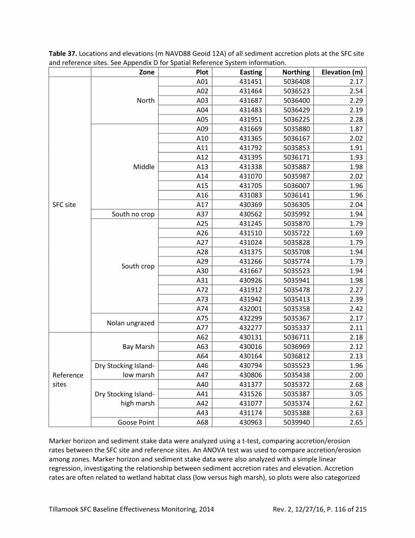
Tillamook SFC Baseline Effectiveness Monitoring, 2014 Rev. 2, 12/27/16, P. 116 of 215
Table 37. Locations and elevations (m NAVD88 Geoid 12A) of all sediment accretion plots at the SFC site and reference sites. See Appendix D for Spatial Reference System information.
Zone Plot Easting Northing Elevation (m)
SFC site
North
A01 431451 5036408 2.17
A02 431464 5036523 2.54
A03 431687 5036400 2.29
A04 431483 5036429 2.19
A05 431951 5036225 2.28
Middle
A09 431669 5035880 1.87
A10 431365 5036167 2.02
A11 431792 5035853 1.91
A12 431395 5036171 1.93
A13 431338 5035887 1.98
A14 431070 5035987 2.02
A15 431705 5036007 1.96
A16 431083 5036141 1.96
A17 430369 5036305 2.04
South no crop A37 430562 5035992 1.94
South crop
A25 431245 5035870 1.79
A26 431510 5035722 1.69
A27 431024 5035828 1.79
A28 431375 5035708 1.94
A29 431266 5035774 1.79
A30 431667 5035523 1.94
A31 430926 5035941 1.98
A72 431912 5035478 2.27
A73 431942 5035413 2.39
A74 432001 5035358 2.42
Nolan ungrazed A75 432299 5035367 2.17
A77 432277 5035337 2.11
Reference sites
Bay Marsh
A62 430131 5036711 2.18
A63 430016 5036969 2.12
A64 430164 5036812 2.13
Dry Stocking Island- low marsh
A46 430794 5035523 1.96
A47 430806 5035438 2.00
Dry Stocking Island-high marsh
A40 431377 5035372 2.68
A41 431526 5035387 3.05
A42 431077 5035374 2.62
A43 431174 5035388 2.63
Goose Point A68 430963 5039940 2.65
Marker horizon and sediment stake data were analyzed using a t-test, comparing accretion/erosion rates between the SFC site and reference sites. An ANOVA test was used to compare accretion/erosion among zones. Marker horizon and sediment stake data were also analyzed with a simple linear regression, investigating the relationship between sediment accretion rates and elevation. Accretion rates are often related to wetland habitat class (low versus high marsh), so plots were also categorized

Tillamook SFC Baseline Effectiveness Monitoring, 2014 Rev. 2, 12/27/16, P. 117 of 215
into low or high marsh by relating plot elevations to the MHHW tidal datum (Figure 13) determined from local water level analysis, and data were analyzed with a two way ANOVA, comparing rates between low and high marsh for the SFC site and reference sites. Since the SFC site is currently diked, tidal influence is absent, so this comparison will likely be more interesting after project implementation. All analyses were completed in R (Version 3.1.1). When distributions did not meet the normality assumptions, an equivalent non-parametric test was used (either a Wilcoxon in place of a t-test or Kruskal-Wallis in place of ANOVA).
Feldspar marker horizon method
Feldspar is a white-colored mineral recommend for use as a marker horizon, as it is highly visible compared to the dark soils present in wetlands (Cahoon et al. 2000). In November 2013, a 5-15 mm layer of feldspar was spread over a 0.25 m2 area in the center of a larger demarcated plot (1 m2). The corners of the 1 m2 plot were marked with PVC poles. A year later (November 2014), we returned to the plots with a pressurized canister (“Dewar”) full of liquid nitrogen. The liquid nitrogen was used to freeze the soil in two sample cores at each plot using the “cryo-coring” method (Cahoon et al. 1996). For each core, four replicate measurements were taken of the amount of material accreted (distance from the top of soil to top of feldspar layer) (Photo 1). Each core was then returned to its initial location in the ground and the core location was recorded to ensure that specific core location would not be re-sampled in future years of monitoring.
Photo 1. Example of field photo showing a feldspar marker horizon core and its sample number. A photo like this was taken of each core, for archival purposes. Sediment to the left of the white feldspar marker horizon has been deposited over the past year.
Sediment stake method
In November 2013, directly adjacent to each feldspar marker horizon plot, two sediment stakes (PVC pipe 2.5 cm diameter, 1 m length, schedule 40) were placed 1 m apart and driven deeply into the ground
Tillamook SFC Baseline Effectiveness Monitoring, 2014 Rev. 2, 12/27/16, P. 118 of 215
and leveled. Using a meter stick laid horizontally across both stake tops, a vertical measurement was taken to the ground surface every 10 cm and measurements were averaged to get a mean measurement per plot and an estimate of standard error. In November 2014 (one year later), this method was repeated, and the difference between November 2013 and November 2014 was calculated, yielding an accretion/erosion rate (mm/year). Erosion was indicated when the difference between the measurements was negative, and accretion was indicated when the difference between the measurement was positive. Sediment stakes were not intended to provide precise measurements of small changes in sediment accretion, but rather provided back-up for the feldspar marker horizon plots if, for example, the feldspar layer was washed away, or if there was significant erosion at a site, since erosion cannot be measured using the feldspar marker horizon method.
Results and discussion There were no significant differences between the SFC site and reference sites in accretion rates, regardless of the method used (feldspar method p = 0.1; sediment stake method p = 0.5) (Figure 74, Figure F1). Sediment accretion rates also did not differ significantly among zones (feldspar method p = 0.5; sediment stake method p = 0.6) (Table 38, Figure 75, Figure F2). Using the feldspar marker horizon method, the SFC site and reference sites had average sediment accretion rates of 7.2 mm/yr and 2.9 mm/yr, respectively. Table 38. Average and standard error of sediment accretion within zones at the SFC site and reference sites for the feldspar marker horizon method. Standard errors could not be calculated for South zone – no crop or Goose Point (n = 1).
Zone Average sediment accretion rate,
mm/yr (standard error)
SFC site
North zone 13.2 (7.2)
Middle zone 6.5 (2.3)
South zone no crop 10.6 (NA)
South zone crop 4.9 (1.4)
Nolan ungrazed 4.7 (2.9)
Reference sites
Bay Marsh 6.0 (1.4)
Dry Stocking Island – low marsh 2.3 (1.0)
Dry Stocking Island – high marsh 1.3 (1.0)
Goose Point 1.8 (NA)
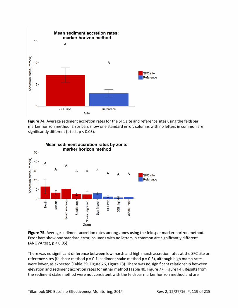
Tillamook SFC Baseline Effectiveness Monitoring, 2014 Rev. 2, 12/27/16, P. 119 of 215
Figure 74. Average sediment accretion rates for the SFC site and reference sites using the feldspar marker horizon method. Error bars show one standard error; columns with no letters in common are significantly different (t-test, p < 0.05).
Figure 75. Average sediment accretion rates among zones using the feldspar marker horizon method. Error bars show one standard error; columns with no letters in common are significantly different (ANOVA test, p < 0.05). There was no significant difference between low marsh and high marsh accretion rates at the SFC site or reference sites (feldspar method p = 0.1, sediment stake method p = 0.5), although high marsh rates were lower, as expected (Table 39, Figure 76, Figure F3). There was no significant relationship between elevation and sediment accretion rates for either method (Table 40, Figure 77, Figure F4). Results from the sediment stake method were not consistent with the feldspar marker horizon method and are
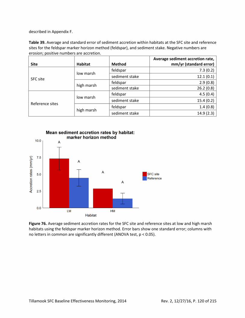
Tillamook SFC Baseline Effectiveness Monitoring, 2014 Rev. 2, 12/27/16, P. 120 of 215
described in Appendix F. Table 39. Average and standard error of sediment accretion within habitats at the SFC site and reference sites for the feldspar marker horizon method (feldspar), and sediment stake. Negative numbers are erosion; positive numbers are accretion.
Site Habitat Method Average sediment accretion rate,
mm/yr (standard error)
SFC site
low marsh feldspar 7.3 (0.2)
sediment stake 12.1 (0.1)
high marsh feldspar 2.9 (0.8)
sediment stake 26.2 (0.8)
Reference sites
low marsh feldspar 4.5 (0.4)
sediment stake 15.4 (0.2)
high marsh feldspar 1.4 (0.8)
sediment stake 14.9 (2.3)
Figure 76. Average sediment accretion rates for the SFC site and reference sites at low and high marsh habitats using the feldspar marker horizon method. Error bars show one standard error; columns with no letters in common are significantly different (ANOVA test, p < 0.05).
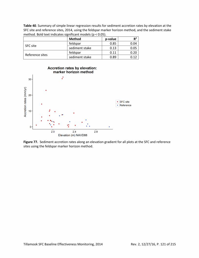
Tillamook SFC Baseline Effectiveness Monitoring, 2014 Rev. 2, 12/27/16, P. 121 of 215
Table 40. Summary of simple linear regression results for sediment accretion rates by elevation at the SFC site and reference sites, 2014, using the feldspar marker horizon method, and the sediment stake method. Bold text indicates significant models (p < 0.05).
Method p-value R2
SFC site feldspar 0.85 0.04
sediment stake 0.13 0.05
Reference sites feldspar 0.11 0.20
sediment stake 0.89 0.12
Figure 77. Sediment accretion rates along an elevation gradient for all plots at the SFC and reference sites using the feldspar marker horizon method.
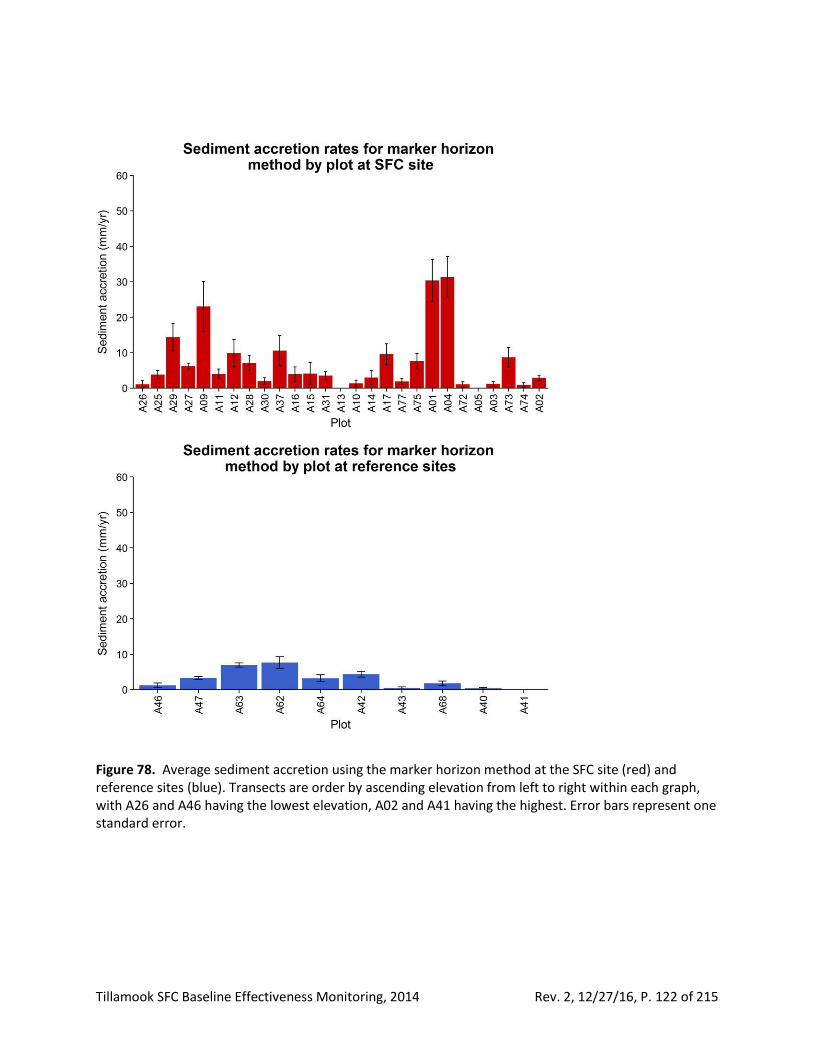
Tillamook SFC Baseline Effectiveness Monitoring, 2014 Rev. 2, 12/27/16, P. 122 of 215
Figure 78. Average sediment accretion using the marker horizon method at the SFC site (red) and reference sites (blue). Transects are order by ascending elevation from left to right within each graph, with A26 and A46 having the lowest elevation, A02 and A41 having the highest. Error bars represent one standard error.
Tillamook SFC Baseline Effectiveness Monitoring, 2014 Rev. 2, 12/27/16, P. 123 of 215
While not statistically significant due to high sample variability, there appeared to be a fairly consistent trend of higher sediment accretion at lower marsh elevations and lower sediment accretion at higher elevations at both the SFC site and reference sites. Other studies have emphasized dramatic differences in accretion rates between low marsh and high marsh habitats, and most tidal wetland development models and West Coast observations show lower accretion rates in high marsh compared to low marsh (Allen 1990, Thom 1992, Simenstad and Thom 1996, Borde et al. 2011). Figure 77 shows sediment accretion rates by sample elevation and Figure 78 shows accretion rates at each individual plot at both the SFC site and reference sites; both figures indicate the variability in the relationship between elevation and accretion rates. The lack of a strong relationship between elevation and sediment accretion at the SFC site was not unexpected, as the SFC site is disconnected from a large proportion of its historic tidal and fluvial sediment sources due to the site’s dikes and tide gates, which disrupt sediment deposition. The lack of a strong elevation – accretion rate correlation at the reference sites was probably due to low sample number (1 to 4 samples per site). The high sediment accretion rates observed within the SFC site were surprising. Although Tillamook Bay has a high sediment supply and high rates of sediment deposition (Philip Williams and Associates 2002), we expected the SFC site to have relatively low accretion rates compared to the reference sites, due to the dikes and tide gates blocking tidal influence from the SFC site. We found instead that the SFC site and reference sites had similar accretion rates. The SFC site had much higher rates of accretion compared to Waite Ranch in the Siuslaw River Estuary, Oregon (Brophy et al. 2015). Both Waite Ranch and the SFC site are currently unrestored, diked agricultural fields, yet the SFC site had an average sediment accretion rate of 7.2 mm/yr, compared to the rate at Waite Ranch, with an accretion rate of 0.6 mm/yr (Brophy et al. 2015). The high sediment accretion rates at the SFC site may indicate substantial sediment movement behind the dike, or sediment transport into the site despite the dikes. The SFC site floods regularly due to heavy rainfall, and flood events sometimes overtop the dikes (see Wetland surface elevation and water levels). These flood events can carry river-transported sediment into the site, and the strong winter winds that generally accompany Pacific Northwest precipitation events can redistribute sediment already present at the site, leading to accretion in some locations and erosion in others. However, we did not observe erosion, nor did the sediment stake method reveal substantial erosion at any location within the SFC site (see Appendix F). Our channel morphology monitoring showed thick layers of fine sediment in channels at the SFC site, but little fine sediment in channels at the reference site (see Channel morphology below). The abundant fine sediments in the SFC channels may have provided a source for sediment redistribution within the SFC site, although we did not observe high flow velocities that might lead to high rates of sediment movement. In summary, the specific mechanisms for the high accretion rates at the SFC site are unknown, but these high accretion rates probably reflect the same forces operating on Tillamook Bay as a whole (Philip Williams and Associates 2002). Sediment accretion rates at the SFC site and reference sites were, on average, higher than reference sites in the Siuslaw River Estuary (Brophy et al. 2015), which averaged around 5.1 mm/yr, as well as higher than rates from other studies of sediment accretion in the PNW, which ranged from 1.8 – 5.8 mm/yr (Rybczyk et al. 2011). These rates reflect the high sediment loads in Tillamook Bay, as described above (Philip Williams and Associates 2002). After tidal reconnection at the SFC site, we expect to see even higher rates of sediment accretion, as restored tidal exchange transports marine and fluvial (river-borne) sediment into the site. Studies in the Columbia River Estuary have shown that after restoration, sediment accretion rates at restoration sites can exceed those at the reference sites, due to lower elevations at the subsided restoration sites (Borde
Tillamook SFC Baseline Effectiveness Monitoring, 2014 Rev. 2, 12/27/16, P. 124 of 215
et al. 2011) and resulting increased “accommodation space” for sediment deposition. Sediment accretion within has been little studied in the Pacific Northwest, and comparisons between diked former tidal wetlands and least-disturbed reference sites have been lacking. Our data help to fill these data gaps, leading to better understanding of tidal wetland physical processes and resilience to climate change.
Linked monitoring of biological and physical parameters One of the SFC project’s ecological goals included increased complexity and availability of tidal wetland habitats. To evaluate this goal, we linked monitoring of biological and physical characteristics that define those habitats and indicate their functions. We co-located the monitoring of a subset of vegetation plots with sediment accretion, soil, groundwater, and elevation monitoring at the SFC site and reference sites, which allowed for the analysis of relationships among these parameters.
Methods Fourteen “clustered vegetation plots” were co-located with the monitoring of sediment accretion plots, soil core samples, groundwater wells, and elevation measurements in 2014 (Table 23, Maps A13 and A17). “Clustered vegetation plots” consisted of four randomly placed vegetation quadrats within 3 m of the groundwater well; these were sampled as described in the Emergent vegetation section. Species richness, native, non-native, and total percent cover were averaged across the four subplots to yield an average per “clustered plot”. Methods for sediment accretion, soil, groundwater, and elevation monitoring are described in the respective sections above. Thirty-seven sediment accretion plots were co-located with vegetation plots, allowing for the exploration of relationships between plant community composition and accretion rates (Table 37, Maps A14 and A16-A17). A multivariate technique, non-metric multidimensional scaling (NMDS), was used to summarize and visualize differences in plant community composition between the SFC site and reference sites, and included only species with greater than 5% cover. Environmental variables contributing to the plant community groupings were determined using the Envfit function in R. Environmental variables included in the analysis were elevation, daily maximum groundwater level, soil pH, soil salinity, soil carbon content, and sediment accretion rates. The NMDS analysis was completed in R (Version 3.1.1) using percent cover per plot as the dependent variable and using the R package vegan (Version 2.1.1). A simple linear regression was used to determine relationships between parameters of interest. (The reference sites only had two clustered plots, therefore regressions could not be run for the reference sites) All analyses were completed in R (Version 3.1.1). When distributions did not meet the normality assumptions, an equivalent non-parametric test was used (either a Wilcoxon in place of a t-test or Kruskal-Wallis in place of ANOVA).
Results and discussion The NMDS showed that all individual vegetation plots at the SFC site grouped together; similarly, all individual vegetation plots at the reference sites grouped together (stress = 0.06; Figure 79). Elevation, soil pH, and soil salinity, were the significant environmental variables contributing to plant community compositions (all p values < 0.001).Over time we expect the NMDS analysis to show convergence between the vegetation plots at the SFC site and the plots at the reference sites

Tillamook SFC Baseline Effectiveness Monitoring, 2014 Rev. 2, 12/27/16, P. 125 of 215
Though multiple relationships were explored across parameters (Table 41), the only significant relationship was between species richness and elevation (see Emergent vegetation for more details). This result is largely due to the homogeneity in physical conditions across the SFC site (i.e., there are no gradients present). Elevations were similar across the site (Table 17, Maps A20), and this was probably the case prior to agricultural conversion of the site, as the whole site was occupied by tidal marsh (Hawes et al. 2008). After tidal reconnection, we expect to see the development of a salinity gradients, which is likely to result in gradients in vegetation and other biotic responses (see Channel water salinity and temperature above).
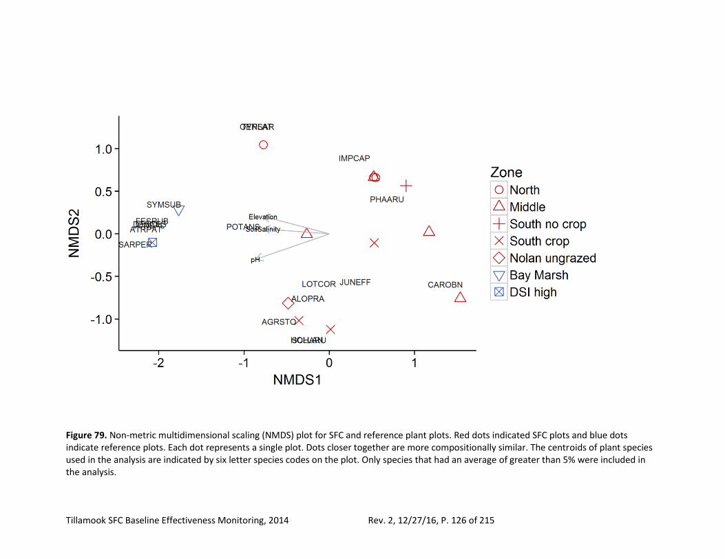
Tillamook SFC Baseline Effectiveness Monitoring, 2014 Rev. 2, 12/27/16, P. 126 of 215
Figure 79. Non-metric multidimensional scaling (NMDS) plot for SFC and reference plant plots. Red dots indicated SFC plots and blue dots indicate reference plots. Each dot represents a single plot. Dots closer together are more compositionally similar. The centroids of plant species used in the analysis are indicated by six letter species codes on the plot. Only species that had an average of greater than 5% were included in the analysis.
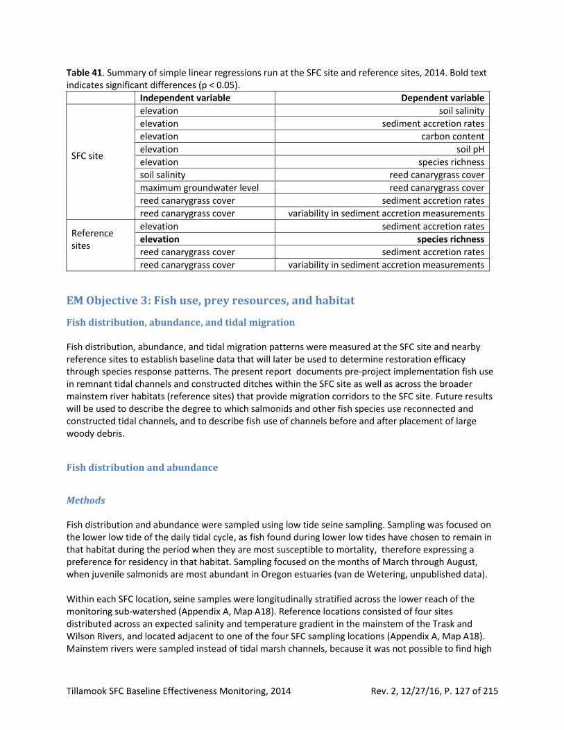
Tillamook SFC Baseline Effectiveness Monitoring, 2014 Rev. 2, 12/27/16, P. 127 of 215
Table 41. Summary of simple linear regressions run at the SFC site and reference sites, 2014. Bold text indicates significant differences (p < 0.05).
Independent variable Dependent variable
SFC site
elevation soil salinity
elevation sediment accretion rates
elevation carbon content
elevation soil pH
elevation species richness
soil salinity reed canarygrass cover
maximum groundwater level reed canarygrass cover
reed canarygrass cover sediment accretion rates
reed canarygrass cover variability in sediment accretion measurements
Reference sites
elevation sediment accretion rates
elevation species richness
reed canarygrass cover sediment accretion rates
reed canarygrass cover variability in sediment accretion measurements
EM Objective 3: Fish use, prey resources, and habitat
Fish distribution, abundance, and tidal migration Fish distribution, abundance, and tidal migration patterns were measured at the SFC site and nearby reference sites to establish baseline data that will later be used to determine restoration efficacy through species response patterns. The present report documents pre-project implementation fish use in remnant tidal channels and constructed ditches within the SFC site as well as across the broader mainstem river habitats (reference sites) that provide migration corridors to the SFC site. Future results will be used to describe the degree to which salmonids and other fish species use reconnected and constructed tidal channels, and to describe fish use of channels before and after placement of large woody debris.
Fish distribution and abundance
Methods Fish distribution and abundance were sampled using low tide seine sampling. Sampling was focused on the lower low tide of the daily tidal cycle, as fish found during lower low tides have chosen to remain in that habitat during the period when they are most susceptible to mortality, therefore expressing a preference for residency in that habitat. Sampling focused on the months of March through August, when juvenile salmonids are most abundant in Oregon estuaries (van de Wetering, unpublished data). Within each SFC location, seine samples were longitudinally stratified across the lower reach of the monitoring sub-watershed (Appendix A, Map A18). Reference locations consisted of four sites distributed across an expected salinity and temperature gradient in the mainstem of the Trask and Wilson Rivers, and located adjacent to one of the four SFC sampling locations (Appendix A, Map A18). Mainstem rivers were sampled instead of tidal marsh channels, because it was not possible to find high

Tillamook SFC Baseline Effectiveness Monitoring, 2014 Rev. 2, 12/27/16, P. 128 of 215
marsh channel reference habitats comparable to the SFC site when geography and human disturbance patterns were considered. Additionally, past experience has shown that to generate fish numbers that allow for reasonable statistical inferences to be made, fish densities have to be at levels commonly found in the mainstem river. Lastly, virtually all fish inhabiting the SFC site are produced outside of the site (in the Tillamook, Trask, Wilson, or Kilchis basins), and use these rivers as corridors for migration – i.e., the rivers are the supply source for the SFC site and therefore allow us to better determine what changes observed during the post-restoration period can be attributed to the restoration itself, as opposed to changes in fish abundance across the full watershed. Within each sample location, a series of samples were taken; each sample consisted of a single seine set. Six seine samples were taken at each SFC sampling location. Five seine samples were taken at each of the three river reference locations. A fourth river reference location was split into two sub-locations, with three seine samples in each sub-location. Sampling at all monitoring locations was standardized by taking all samples during the morning lower low slack tide, using the same net for each location, and sampling the same surface area each time. We were unable to take samples at Dry stocking Island due to its higher channel bed elevation and absence of water in the channel during low tide sampling. Mainstem reference samples consisted of a seine set that measured 10 m in length and varied slightly in width, averaging five meters, with an average max depth of 1.5 m and minimum depth of 0 m. All channel seine sets at the SFC site were 10 m in length and up to 10 m in width, or the width of the wetted channel if it measured less than 10 m. SFC site channel seine-set depths averaged 0.1 m ranging from 0.05 to 1.5 m. We calculated catch per unit effort (CPUE) for each sample at each sample location. CPUE is an indirect measure of the abundance of a target species based on repeated sampling using standardized methods (Sutherland 2000). Changes in the CPUE are inferred to signify changes to the target species' true abundance. CPUE has been used for fisheries monitoring for several years (Maundera 2006). Our seine capture data (i.e., individual sample fish counts) are hereinafter referred to as CPUE. Because we observed several species across three seasons, and several species had periods of absence and periods of peak use, zero-count CPUE values were a common occurrence (Tables 42 and 43). Treatment of each sample at each location as a unique sample to be used to calculate a mean CPUE can create possible violations in assumptions of independence, therefore we chose a simple and direct method of evaluation. We examined the species age-class groups during three key periods (early spring [March through April] late spring [May through April], and summer [July through August]) and analyzed the sum of each location’s CPUE samples for a particular day rather than the mean. The sum of each location’s samples for a given day was defined as a visit with a total count. There were 17 visits in early spring, 17 visits in late spring, and 15 visits in summer. The number of samples completed during a visit varied from three to six based on whether it was one of the two sub-locations (where the target N=3), a river reference location (target N=5) or a wetland location (target N=6). We used the number of samples in a visit as an offset in the model to account for unequal effort. Because we were modeling count data with log-linear models (either Poisson or negative binomial), the offset was included as the natural logarithm of the number of samples. Counts for age-1 Coho in summer, age-0 Chum in late spring and summer, Prickly sculpin in early and late spring, and age-0 and age-1 Shiner perch in early and late spring were all zeros (Tables 42 & 43), though they were not expected to be present. Since they were not expected to be present and did not show up in the survey during specific months, we analyzed age-1 Coho CPUE during early spring only,
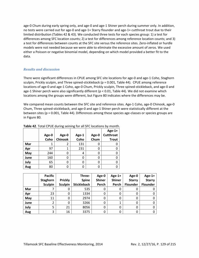
Tillamook SFC Baseline Effectiveness Monitoring, 2014 Rev. 2, 12/27/16, P. 129 of 215
age-0 Chum during early spring only, and age-0 and age-1 Shiner perch during summer only. In addition, no tests were carried out for age-0 and age-1+ Starry flounder and age-1+ cutthroat trout due to their limited distribution (Tables 42 & 43). We conducted three tests for each species group: 1) a test for differences among SFC location counts; 2) a test for differences among reference location counts; and 3) a test for differences between counts at the SFC site versus the reference sites. Zero-inflated or hurdle models were not needed because we were able to eliminate the excessive amount of zeros. We used either a Poisson or negative binomial model, depending on which model provided a better fit to the data. Results and discussion There were significant differences in CPUE among SFC site locations for age-0 and age-1 Coho, Staghorn sculpin, Prickly sculpin, and Three spined-stickleback (p = 0.001, Table 44). CPUE among reference locations of age-0 and age-1 Coho, age-0 Chum, Prickly sculpin, Three spined-stickleback, and age-0 and age-1 Shiner perch were also significantly different (p < 0.01, Table 44). We did not examine which locations among the groups were different, but Figure 80 indicates where the differences may be. We compared mean counts between the SFC site and reference sites. Age-1 Coho, age-0 Chinook, age-0 Chum, Three spined-stickleback, and age-0 and age-1 Shiner perch were statistically different at the between sites (p = 0.001, Table 44). Differences among these species age-classes or species groups are in Figure 80. Table 42. Total CPUE during seining for all SFC locations by month.
Age-0 Coho
Age-0 Chinook
Age-1 Coho
Age-0 Chum
Age-1+ Cutthroat
Trout
Mar 1 2 131 0 0
Apr 97 1 231 0 0
May 244 0 4 0 0
June 160 0 0 0 0
July 65 0 0 0 0
Aug 80 0 0 0 0
Pacific Staghorn
Sculpin Prickly
Sculpin
Three- Spine
Stickleback
Age-0 Shiner Perch
Age-1+ Shiner Perch
Age-0 Starry
Flounder
Age-1+ Starry
Flounder
Mar 7 0 535 0 0 0 0
Apr 23 0 1334 0 0 0 0
May 11 0 2974 0 0 0 0
June 2 0 3266 0 1 0 0
July 5 21 8056 0 0 0 0
Aug 3 16 3375 0 0 0 0

Tillamook SFC Baseline Effectiveness Monitoring, 2014 Rev. 2, 12/27/16, P. 130 of 215
Table 43. Total fish captured during seining for all mainstem river reference locations by month.
Age-0 Coho
Age-0 Chinook
Age-1 Coho
Age-0 Chum
Age-1+ Cutthroat
Trout
Mar 13 0 0 0 2 Apr 66 51 33 78 0 May 30 616 57 0 0 June 1 222 0 0 2 July 4 166 0 0 5 Aug 0 90 0 0 0
Pacific Staghorn
Sculpin Prickly
Sculpin
Three- Spined
Stickleback
Age-0 Shiner Perch
Age-1+ Shiner Perch
Age-0 Starry
Flounder
Age-1+ Starry
Flounder
Mar 29 0 6 0 0 3 4
Apr 50 0 67 0 0 4 14
May 33 0 530 0 0 0 3
June 123 0 83 0 0 10 4
July 193 0 39 108 193 6 10
Aug 88 33 1 344 30 37 2
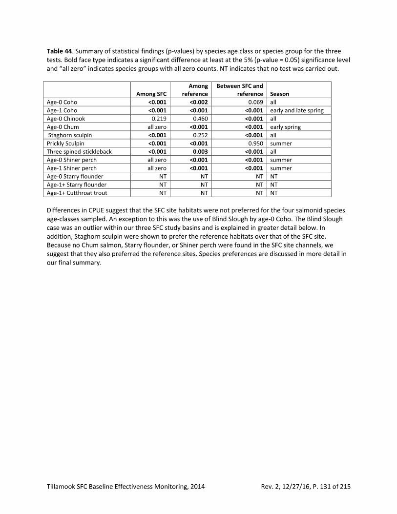
Tillamook SFC Baseline Effectiveness Monitoring, 2014 Rev. 2, 12/27/16, P. 131 of 215
Table 44. Summary of statistical findings (p-values) by species age class or species group for the three tests. Bold face type indicates a significant difference at least at the 5% (p-value = 0.05) significance level and “all zero” indicates species groups with all zero counts. NT indicates that no test was carried out.
Among SFC
Among reference
Between SFC and reference Season
Age-0 Coho <0.001 <0.002 0.069 all
Age-1 Coho <0.001 <0.001 <0.001 early and late spring
Age-0 Chinook 0.219 0.460 <0.001 all
Age-0 Chum all zero <0.001 <0.001 early spring
Staghorn sculpin <0.001 0.252 <0.001 all
Prickly Sculpin <0.001 <0.001 0.950 summer
Three spined-stickleback <0.001 0.003 <0.001 all
Age-0 Shiner perch all zero <0.001 <0.001 summer
Age-1 Shiner perch all zero <0.001 <0.001 summer
Age-0 Starry flounder NT NT NT NT
Age-1+ Starry flounder NT NT NT NT
Age-1+ Cutthroat trout NT NT NT NT
Differences in CPUE suggest that the SFC site habitats were not preferred for the four salmonid species age-classes sampled. An exception to this was the use of Blind Slough by age-0 Coho. The Blind Slough case was an outlier within our three SFC study basins and is explained in greater detail below. In addition, Staghorn sculpin were shown to prefer the reference habitats over that of the SFC site. Because no Chum salmon, Starry flounder, or Shiner perch were found in the SFC site channels, we suggest that they also preferred the reference sites. Species preferences are discussed in more detail in our final summary.
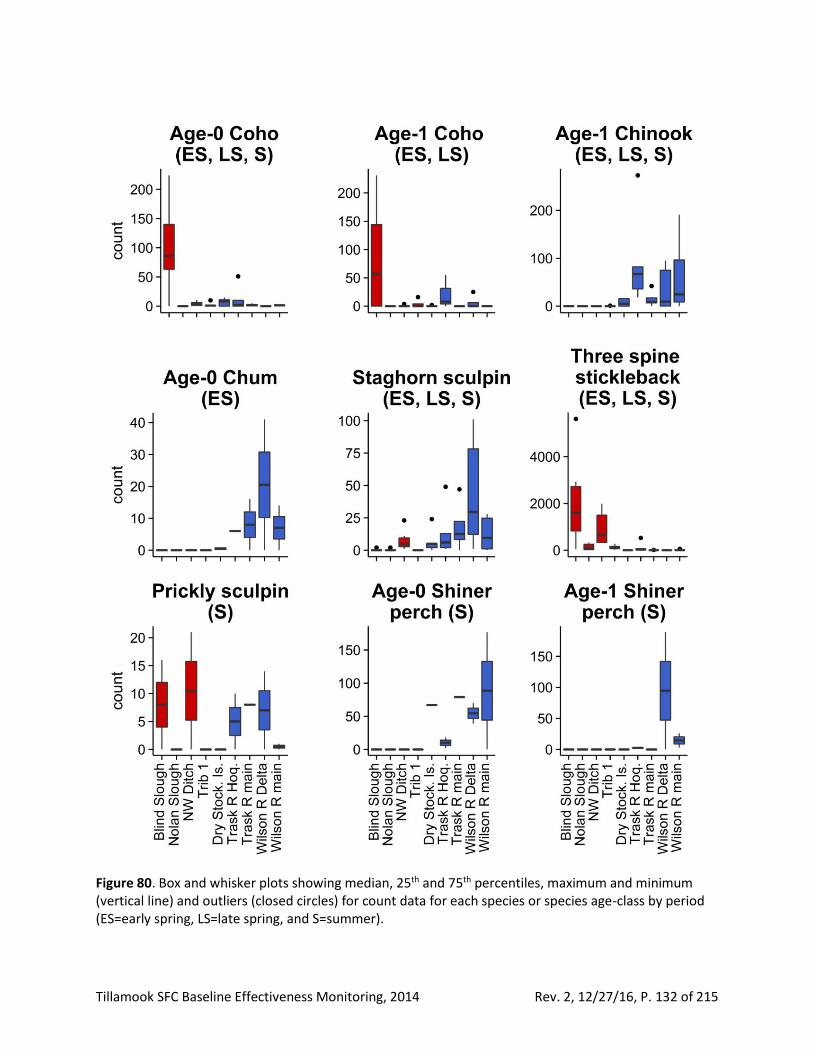
Tillamook SFC Baseline Effectiveness Monitoring, 2014 Rev. 2, 12/27/16, P. 132 of 215
Figure 80. Box and whisker plots showing median, 25th and 75th percentiles, maximum and minimum (vertical line) and outliers (closed circles) for count data for each species or species age-class by period (ES=early spring, LS=late spring, and S=summer).
Tillamook SFC Baseline Effectiveness Monitoring, 2014 Rev. 2, 12/27/16, P. 133 of 215
Tidal migration Methods This monitoring report provides baseline data on fish migration patterns prior to dike and tide gate removal, as well as channel reconstruction and habitat enhancement through wood placement. Post-implementation monitoring will document potential shifts in fish migration patterns across the restored marsh. The focus of the post-implementation work will be to describe how, through daily migrations, fish use the mainstem river and the restored marsh as a series of preferred habitats.
Because age-0 Chinook were present in our 2014 seine samples at much greater numbers than any other salmonid species-age class found at the reference locations, they were designated as the target species for migration evaluations. Age-0 Chinook were present by April, peaked in May, and began to decrease in number by June (Table 43, Figure 80). Based on this pattern, the months of May, June, and July were chosen as migration sampling months. For comparability, sampling during May, June, and July was timed for the same portion of the monthly tidal cycle so fish experienced the same tide heights and timing of the daily cycle. Our target sample tide cycle began with an early morning lower low followed by a 1.8 m (6 ft) late morning lower high, followed by a late afternoon higher low. Two daily tidal cycles were sampled during each sample month. SFC tidal migration sampling occurred inside the mouth of three sub-basin channels (Blind Slough, Nolan Slough, and NW Ditch) (Appendix A, Map A18). Sampling during the pre-restoration period at tide gate locations occurred approximately 10 m inside the upstream end of the tide gate pipe itself. This allowed the commonly occurring tide pipe “headwater pool” to be included downstream of the sampling transect. Fish migration sampling was completed using a “fence” of cameras (sampling transect) positioned perpendicular to the channel (Figure 81). Fyke nets nets were used to narrow the channel’s width to that of the tide pipe (Figure 81 and Appendix B, Figure B17). Stations were located 0.3 m apart. There were two stations per sample location. River reference location sampling occurred along the banks of the Wilson River, Wilson River Side Channel, and Trask River (Appendix A, Map A18). Mainstem river bank reference sampling occurred just downstream of the mouth of the adjacent SFC study channel. Reference sub-basin sampling (Dry Stocking Island channel) occurred at the downstream-most point in the channel, where the channel spilled into the mainstem river (Appendix A, Map A18). Guide nets running from the bank toward the thalweg were used to concentrate and direct migrating fish toward the camera sampling transect (Figure 81 and Appendix B, Figure B17). Sampling transects consisted of a set of poles (stations) positioned in a line perpendicular to water flow. Stations were located 0.3 m apart. There were two stations per sample location.
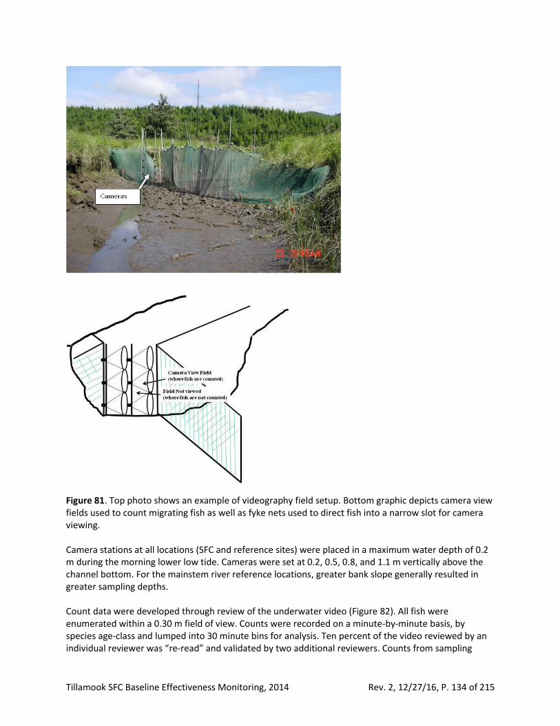
Tillamook SFC Baseline Effectiveness Monitoring, 2014 Rev. 2, 12/27/16, P. 134 of 215
Figure 81. Top photo shows an example of videography field setup. Bottom graphic depicts camera view fields used to count migrating fish as well as fyke nets used to direct fish into a narrow slot for camera viewing. Camera stations at all locations (SFC and reference sites) were placed in a maximum water depth of 0.2 m during the morning lower low tide. Cameras were set at 0.2, 0.5, 0.8, and 1.1 m vertically above the channel bottom. For the mainstem river reference locations, greater bank slope generally resulted in greater sampling depths. Count data were developed through review of the underwater video (Figure 82). All fish were enumerated within a 0.30 m field of view. Counts were recorded on a minute-by-minute basis, by species age-class and lumped into 30 minute bins for analysis. Ten percent of the video reviewed by an individual reviewer was “re-read” and validated by two additional reviewers. Counts from sampling
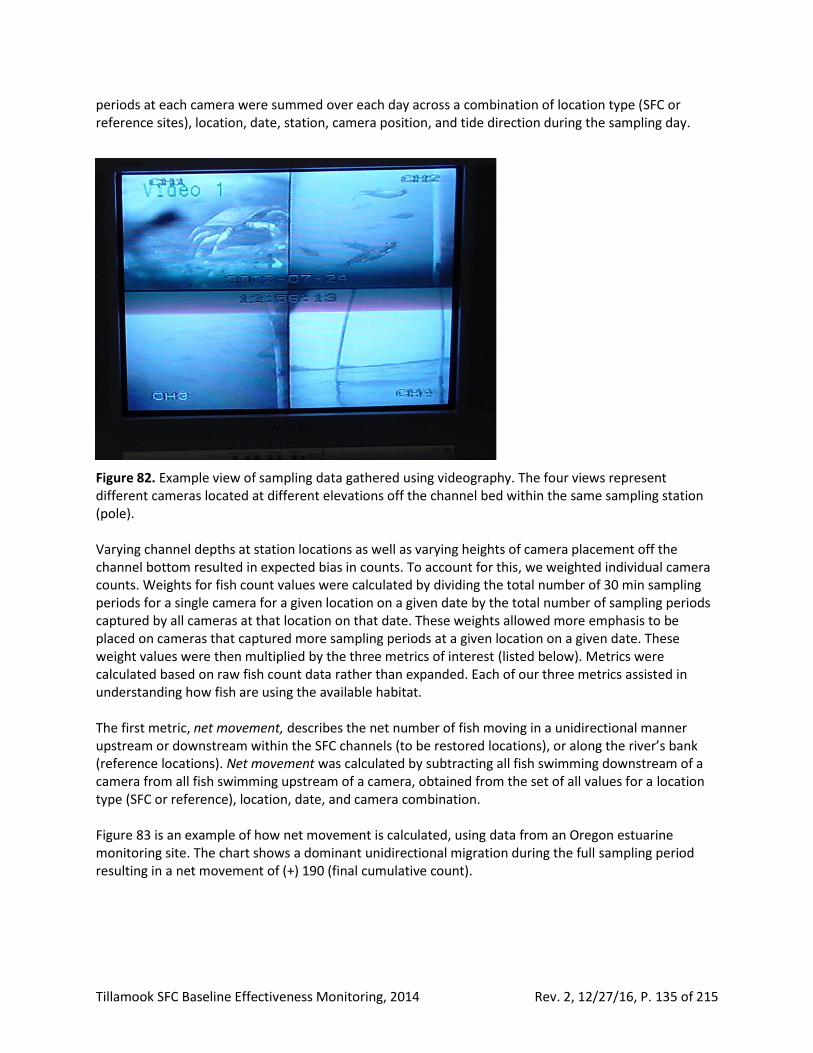
Tillamook SFC Baseline Effectiveness Monitoring, 2014 Rev. 2, 12/27/16, P. 135 of 215
periods at each camera were summed over each day across a combination of location type (SFC or reference sites), location, date, station, camera position, and tide direction during the sampling day.
Figure 82. Example view of sampling data gathered using videography. The four views represent different cameras located at different elevations off the channel bed within the same sampling station (pole). Varying channel depths at station locations as well as varying heights of camera placement off the channel bottom resulted in expected bias in counts. To account for this, we weighted individual camera counts. Weights for fish count values were calculated by dividing the total number of 30 min sampling periods for a single camera for a given location on a given date by the total number of sampling periods captured by all cameras at that location on that date. These weights allowed more emphasis to be placed on cameras that captured more sampling periods at a given location on a given date. These weight values were then multiplied by the three metrics of interest (listed below). Metrics were calculated based on raw fish count data rather than expanded. Each of our three metrics assisted in understanding how fish are using the available habitat. The first metric, net movement, describes the net number of fish moving in a unidirectional manner upstream or downstream within the SFC channels (to be restored locations), or along the river’s bank (reference locations). Net movement was calculated by subtracting all fish swimming downstream of a camera from all fish swimming upstream of a camera, obtained from the set of all values for a location type (SFC or reference), location, date, and camera combination. Figure 83 is an example of how net movement is calculated, using data from an Oregon estuarine monitoring site. The chart shows a dominant unidirectional migration during the full sampling period resulting in a net movement of (+) 190 (final cumulative count).
11
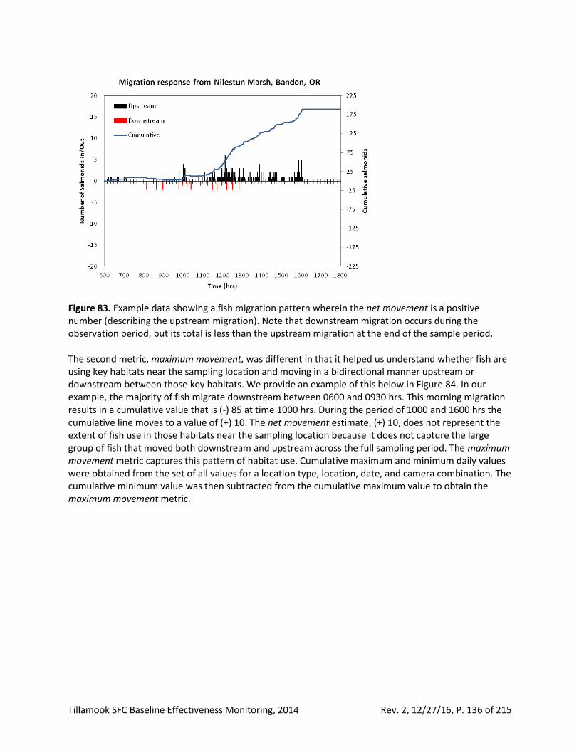
Tillamook SFC Baseline Effectiveness Monitoring, 2014 Rev. 2, 12/27/16, P. 136 of 215
Figure 83. Example data showing a fish migration pattern wherein the net movement is a positive number (describing the upstream migration). Note that downstream migration occurs during the observation period, but its total is less than the upstream migration at the end of the sample period. The second metric, maximum movement, was different in that it helped us understand whether fish are using key habitats near the sampling location and moving in a bidirectional manner upstream or downstream between those key habitats. We provide an example of this below in Figure 84. In our example, the majority of fish migrate downstream between 0600 and 0930 hrs. This morning migration results in a cumulative value that is (-) 85 at time 1000 hrs. During the period of 1000 and 1600 hrs the cumulative line moves to a value of (+) 10. The net movement estimate, (+) 10, does not represent the extent of fish use in those habitats near the sampling location because it does not capture the large group of fish that moved both downstream and upstream across the full sampling period. The maximum movement metric captures this pattern of habitat use. Cumulative maximum and minimum daily values were obtained from the set of all values for a location type, location, date, and camera combination. The cumulative minimum value was then subtracted from the cumulative maximum value to obtain the maximum movement metric.
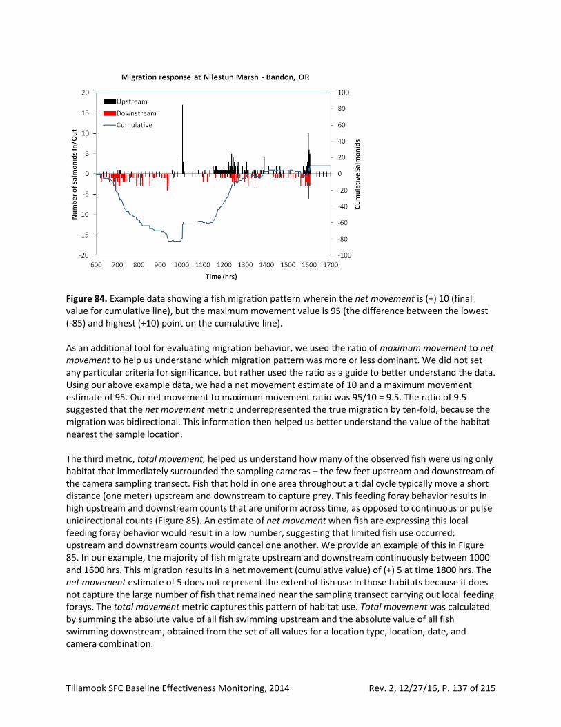
Tillamook SFC Baseline Effectiveness Monitoring, 2014 Rev. 2, 12/27/16, P. 137 of 215
Figure 84. Example data showing a fish migration pattern wherein the net movement is (+) 10 (final value for cumulative line), but the maximum movement value is 95 (the difference between the lowest (-85) and highest (+10) point on the cumulative line). As an additional tool for evaluating migration behavior, we used the ratio of maximum movement to net movement to help us understand which migration pattern was more or less dominant. We did not set any particular criteria for significance, but rather used the ratio as a guide to better understand the data. Using our above example data, we had a net movement estimate of 10 and a maximum movement estimate of 95. Our net movement to maximum movement ratio was 95/10 = 9.5. The ratio of 9.5 suggested that the net movement metric underrepresented the true migration by ten-fold, because the migration was bidirectional. This information then helped us better understand the value of the habitat nearest the sample location. The third metric, total movement, helped us understand how many of the observed fish were using only habitat that immediately surrounded the sampling cameras – the few feet upstream and downstream of the camera sampling transect. Fish that hold in one area throughout a tidal cycle typically move a short distance (one meter) upstream and downstream to capture prey. This feeding foray behavior results in high upstream and downstream counts that are uniform across time, as opposed to continuous or pulse unidirectional counts (Figure 85). An estimate of net movement when fish are expressing this local feeding foray behavior would result in a low number, suggesting that limited fish use occurred; upstream and downstream counts would cancel one another. We provide an example of this in Figure 85. In our example, the majority of fish migrate upstream and downstream continuously between 1000 and 1600 hrs. This migration results in a net movement (cumulative value) of (+) 5 at time 1800 hrs. The net movement estimate of 5 does not represent the extent of fish use in those habitats because it does not capture the large number of fish that remained near the sampling transect carrying out local feeding forays. The total movement metric captures this pattern of habitat use. Total movement was calculated by summing the absolute value of all fish swimming upstream and the absolute value of all fish swimming downstream, obtained from the set of all values for a location type, location, date, and camera combination.
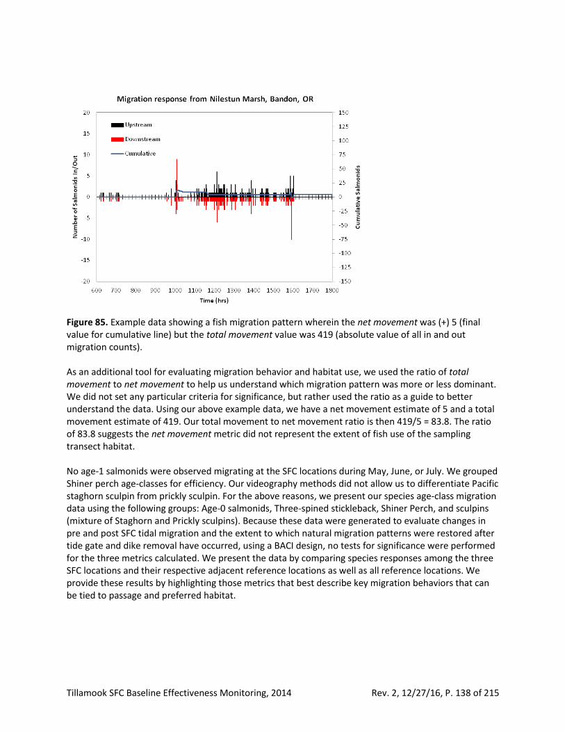
Tillamook SFC Baseline Effectiveness Monitoring, 2014 Rev. 2, 12/27/16, P. 138 of 215
Figure 85. Example data showing a fish migration pattern wherein the net movement was (+) 5 (final value for cumulative line) but the total movement value was 419 (absolute value of all in and out migration counts). As an additional tool for evaluating migration behavior and habitat use, we used the ratio of total movement to net movement to help us understand which migration pattern was more or less dominant. We did not set any particular criteria for significance, but rather used the ratio as a guide to better understand the data. Using our above example data, we have a net movement estimate of 5 and a total movement estimate of 419. Our total movement to net movement ratio is then 419/5 = 83.8. The ratio of 83.8 suggests the net movement metric did not represent the extent of fish use of the sampling transect habitat. No age-1 salmonids were observed migrating at the SFC locations during May, June, or July. We grouped Shiner perch age-classes for efficiency. Our videography methods did not allow us to differentiate Pacific staghorn sculpin from prickly sculpin. For the above reasons, we present our species age-class migration data using the following groups: Age-0 salmonids, Three-spined stickleback, Shiner Perch, and sculpins (mixture of Staghorn and Prickly sculpins). Because these data were generated to evaluate changes in pre and post SFC tidal migration and the extent to which natural migration patterns were restored after tide gate and dike removal have occurred, using a BACI design, no tests for significance were performed for the three metrics calculated. We present the data by comparing species responses among the three SFC locations and their respective adjacent reference locations as well as all reference locations. We provide these results by highlighting those metrics that best describe key migration behaviors that can be tied to passage and preferred habitat.

Tillamook SFC Baseline Effectiveness Monitoring, 2014 Rev. 2, 12/27/16, P. 139 of 215
Results and discussion More than 70,000 fish were counted across 2,519 single camera sampling periods (30 min). In general, variance in the counts was low which will increase our ability to measure future differences (pre and post-restoration analyses) with greater statistical power. The SFC Blind Slough sampling transect was in a short section of channel between the upstream end of the tide pipe and the tide pipe’s headwater pool. The earlier described seine sampling showed high numbers of age-0 Coho and Three-spined stickleback living within this headwater pool during several months of the year. This headwater pool was more than ten times the size of the pool associated with the Nolan or NW Ditch tide pipes and more than a meter deeper – note that we do not describe these tide pipe headwater pools in our channel morphology assessments above. The SFC Nolan Slough transect was upstream of the tide pipe’s headwater pool and downstream of limited low tide refugia habitat. The earlier described seine sampling showed no age-0 salmonids residing upstream of this pipe’s headwater pool during several months of the year. The SFC NW Ditch transect was upstream of the tide pipe’s headwater pool and downstream of a few smaller low tide refugia pools. The earlier described seine sampling showed small numbers of age-0 Coho residing upstream of this pipe’s headwater pool during several months of the year.
Age-0 salmonids
• Using mean net movement, we estimated fewer age-0 salmonids migrating at the SFC tide gate locations than at the adjacent reference locations (Table 45).
• The maximum movement to net movement ratios were higher (individual locations and the mean of locations) for the SFC site than for the river reference locations (Table 45).
• The total movement to net movement ratios were higher (individual locations and the mean of locations) for the SFC site when compared to the river reference locations (Table 45).
Three-spined stickleback
• Using mean net movement we estimated more Three-spined stickleback migrating at the SFC tide gate locations than at the adjacent river reference locations (Table 45).
• The maximum movement to net movement ratios were similar (individual locations and the mean of locations) for the SFC site when compared to the river reference locations (Table 45).
• The total movement to net movement ratios were higher at two individual locations and the mean of locations) for the SFC site when compared to the river reference locations (Table 45).
Shiner perch
• Using mean net movement, we estimated fewer Shiner perch migrating at two of the SFC tide gate locations than at the adjacent reference locations (Table 46). The Shiner perch numbers for three SFC locations and one reference location were too low to draw conclusions at this time. The seine data also showed low numbers of Shiner perch within the SFC site and at Wilson River and Trask River reference locations (see above Fish distribution and abundance section).
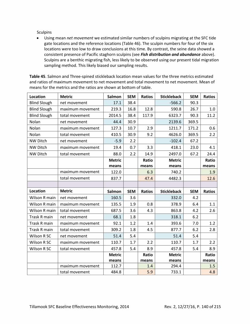
Tillamook SFC Baseline Effectiveness Monitoring, 2014 Rev. 2, 12/27/16, P. 140 of 215
Sculpins
• Using mean net movement we estimated similar numbers of sculpins migrating at the SFC tide gate locations and the reference locations (Table 46). The sculpin numbers for four of the six locations were too low to draw conclusions at this time. By contrast, the seine data showed a consistent presence of Pacific staghorn sculpins (see Fish distribution and abundance above). Sculpins are a benthic migrating fish, less likely to be observed using our present tidal migration sampling method. This likely biased our sampling results.
Table 45. Salmon and Three-spined stickleback location mean values for the three metrics estimated and ratios of maximum movement to net movement and total movement to net movement. Mean of means for the metrics and the ratios are shown at bottom of table.
Location Metric Salmon SEM Ratios Stickleback SEM Ratios
Blind Slough net movement 17.1 38.4 -566.2 90.3
Blind Slough maximum movement 219.3 16.8 12.8 590.8 26.7 1.0
Blind Slough total movement 2014.5 38.4 117.9 6323.7 90.3 11.2
Nolan net movement 44.4 30.9 2139.6 369.5
Nolan maximum movement 127.3 10.7 2.9 1211.7 171.2 0.6
Nolan total movement 410.5 30.9 9.2 4626.0 369.5 2.2
NW Ditch net movement -5.9 2.2 -102.4 67.2
NW Ditch maximum movement 19.4 0.7 3.3 418.1 23.0 4.1
NW Ditch total movement 88.0 2.2 14.9 2497.0 67.2 24.4
Metric means
Ratio means
Metric means
Ratio means
maximum movement 122.0 6.3 740.2 1.9
total movement 837.7 47.4 4482.3 12.6
Location Metric Salmon SEM Ratios Stickleback SEM Ratios
Wilson R main net movement 160.5 3.6 332.0 4.2
Wilson R main maximum movement 135.5 1.9 0.8 378.9 6.4 1.1
Wilson R main total movement 687.5 3.6 4.3 863.8 4.2 2.6
Trask R main net movement 68.1 1.8 318.1 6.2
Trask R main maximum movement 92.1 1.2 1.4 393.6 7.0 1.2
Trask R main total movement 309.2 1.8 4.5 877.7 6.2 2.8
Wilson R SC net movement 51.4 5.4 51.4 5.4
Wilson R SC maximum movement 110.7 1.7 2.2 110.7 1.7 2.2
Wilson R SC total movement 457.8 5.4 8.9 457.8 5.4 8.9
Metric means
Ratio means
Metric means
Ratio means
maximum movement 112.7 1.4 294.4 1.5
total movement 484.8 5.9 733.1 4.8
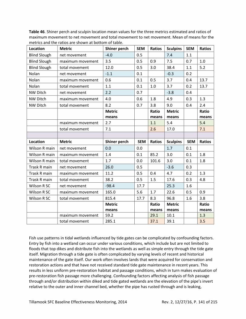
Tillamook SFC Baseline Effectiveness Monitoring, 2014 Rev. 2, 12/27/16, P. 141 of 215
Table 46. Shiner perch and sculpin location mean values for the three metrics estimated and ratios of maximum movement to net movement and total movement to net movement. Mean of means for the metrics and the ratios are shown at bottom of table.
Location Metric Shiner perch SEM Ratios Sculpins SEM Ratios
Blind Slough net movement -4.0 0.5 7.4 1.1
Blind Slough maximum movement 3.5 0.5 0.9 7.5 0.7 1.0
Blind Slough total movement 12.0 0.5 3.0 38.4 1.1 5.2
Nolan net movement -1.1 0.1 -0.3 0.2
Nolan maximum movement 0.6 0.1 0.5 3.7 0.4 13.7
Nolan total movement 1.1 0.1 1.0 3.7 0.2 13.7
NW Ditch net movement 2.2 0.7 -3.8 0.4
NW Ditch maximum movement 4.0 0.6 1.8 4.9 0.3 1.3
NW Ditch total movement 8.2 0.7 3.8 9.0 0.4 2.4
Metric means
Ratio means
Metric means
Ratio means
maximum movement 2.7 1.1 5.4 5.4
total movement 7.1 2.6 17.0 7.1
Location Metric Shiner perch SEM Ratios Sculpins SEM Ratios
Wilson R main net movement 0.0 0.0 1.7 0.1
Wilson R main maximum movement 1.4 0.1 85.2 3.0 0.1 1.8
Wilson R main total movement 1.7 0.0 101.6 3.0 0.1 1.8
Trask R main net movement 26.0 0.5 -3.6 0.3
Trask R main maximum movement 11.2 0.5 0.4 4.7 0.2 1.3
Trask R main total movement 38.2 0.5 1.5 17.6 0.3 4.8
Wilson R SC net movement -98.4 17.7 25.3 1.6
Wilson R SC maximum movement 165.0 5.6 1.7 22.6 0.5 0.9
Wilson R SC total movement 815.4 17.7 8.3 96.8 1.6 3.8
Metric means
Ratio means
Metric means
Ratio means
maximum movement 59.2 29.1 10.1 1.3
total movement 285.1 37.1 39.1 3.5
Fish use patterns in tidal wetlands influenced by tide gates can be complicated by confounding factors. Entry by fish into a wetland can occur under various conditions, which include but are not limited to floods that top dikes and distribute fish into the wetlands as well as simple entry through the tide gate itself. Migration through a tide gate is often complicated by varying levels of recent and historical maintenance of the gate itself. Our work often involves lands that were acquired for conservation and restoration actions and that have not received standard tide gate maintenance in recent years. This results in less uniform pre-restoration habitat and passage conditions, which in turn makes evaluation of pre-restoration fish passage more challenging. Confounding factors affecting analysis of fish passage through and/or distribution within diked and tide gated wetlands are the elevation of the pipe’s invert relative to the outer and inner channel bed, whether the pipe has rusted through and is leaking,

Tillamook SFC Baseline Effectiveness Monitoring, 2014 Rev. 2, 12/27/16, P. 142 of 215
whether water can pass around the outer edge of the pipe, the type of gate and whether it is functional, the extent of low water refugia pools across the wetland, and the water quality of the wetland habitat. We use this information to assist us in interpretation of fish distributions and tidal migration patterns. Our results fit with expectations for the diked, ditched, and hydrologically altered context of the SFC site. The SFC channels surveyed (Blind Slough, Nolan Slough and the NW Ditch network) had significantly altered tidal exchange and habitat conditions (see Wetland surface elevation and water level, Channel water salinity and temperature, and Channel morphology sections above). All three tide gates had tide pipe headwater pools that were deep enough to provide low tide refugia during all months of the year. Each of the gates allowed some exchange of tidal water, albeit limited and for different reasons. Blind Slough had two “early model” side hinged circular tide gates. These allowed for some muted exchange (see Wetland surface elevation and water level section above). In addition, based on anecdotal information (snorkel observations) there appeared to be ground water input or hyporheic exchange resulting in cooler stratified water during the late spring and summer sampling periods. We attempted to differentiate this source and identify the extent of stratification, but were largely unsuccessful due to the relatively shallow depths of the channel. Nolan Slough had an older circular top hinge gate that had not been maintained, which allowed water to flow in via the flap that was stuck open approximately eight inches. Our surface water salinity data reflected this muted tidal regime in Nolan Slough (Figure 27), as did brackish-tolerant vegetation along the banks of lower Nolan Slough (Appendix A, Map A8).The tide gate located at the mouth of the NW Ditch network was also stuck in a partially open position during several months of 2014. A portion of the daily flow that entered Nolan Slough tide gate flowed into the upper reaches of the NW Ditch network due to ditch flow patterns and channel bottom elevations. This provided a constant minimal flow to the NW Ditch channel network working from the upper reaches in a downstream direction. The presence of these tide pipe headwater pools and associated leaky tide gate systems created a confounding factor in that juvenile fish could rear in these pools and will typically complete short daily bidirectional migrations into and out of the tide pipe or headwater pool and/or exhibit high levels of feeding behavior as the tide ebbs and flows through the leaky tide gate. The number of fish and their behavior is typically related to the size of the headwater pool and rate of tidal exchange (van de Wetering, unpublished data). Our results suggest that tide gate presence affected daily tidal migration of age-0 salmonids and Three-spined stickleback. Age-0 salmonid mean net movement was lower at the SFC locations when compared to the adjacent reference locations. Age-0 salmonids observed at SFC locations exhibited greater levels of bidirectional migration and local feeding forays when compared to those at reference locations. Three-spined stickleback mean net movement was higher at SFC locations when compared to those at adjacent reference locations. Three-spined stickleback observed at SFC locations exhibited higher levels of local feeding forays when compared to the reference locations. Daily tidal migrations did not seem to be occurring through the tide gates, even though one location’s gate was fish friendly and the remaining two locations had gates stuck in a partially open position. We could draw only limited conclusions from the migration study for Shiner perch and Pacific Staghorn sculpin at the SFC site, due to the low number of fish observed. However, these two species groups were observed in higher numbers at three of the four migration reference locations during distribution sampling. Results from the distribution study (see Fish distribution and abundance section above) support absence of daily tidal migrations into or out of the SFC locations by Chinook, Chum, sculpins,
Tillamook SFC Baseline Effectiveness Monitoring, 2014 Rev. 2, 12/27/16, P. 143 of 215
Shiner perch, and Starry flounder. Results in our Fish distribution and abundance section also support limited to no SFC tide gate migration by age-0 Coho and Three spined-stickleback.
Summary of fish distribution, abundance and tidal migration The sustained presence of juvenile Coho in a single habitat (Blind Slough) was likely due to the presence of what we refer to as “tidal wetland beaver dam habitat” – deeper pools, adequate water quality (stratified summer temperatures), minimal but daily water exchange (fish friendly tide gate) (Brophy et al. 2014, van de Wetering 2007), and significant food resources such as midges (Chironomidae) (see Prey resources (benthic macroinvertebrates) below). Conversely, we suggest that the limited presence of this species at Nolan Slough and the NW Ditch was a result of the absence of beaver dam habitat. We apply the same site-based conclusions to Three-spined stickleback based on their preference for beaver dam habitat (Brophy et al. 2013). For those species that used tidal channels for daily migrations (Chinook, Pacific Staghorn sculpin, prickly sculpin, Shiner perch, and Starry flounder), we conclude that the tide gate systems of all three SFC locations reduced, if not totally eliminated, daily tidal migration. Both seine and camera sampling results supported this conclusion. As described in our Channel morphology section above, when tidal forces are introduced to the SFC channels following construction of the project, we expect to see morphological shifts towards equilibrium resulting in scour and fill of existing channel habitats. Since the construction elements include removal of the existing passage barriers, we expect to see an increase in daily channel migration by species such as age-0 Chinook, Shiner perch, sculpins, and Starry Flounder. As low tide refugia shift, we expect to see variations in species distributions with increased wetland channel use by age-0 Chinook, Shiner perch, Starry flounder, Pacific Staghorn, and Prickly sculpins, especially where wood creates scour pools. Conversely we expect to see reduced use by age-0 Coho and Three-spined stickleback where removal of existing barriers increases daily tidal exchange. However, if beaver are successful at constructing dams within the restored wetlands, we expect to see Coho use those habitats at high densities.
Prey resources (benthic macroinvertebrates)
Methods Sampling occurred in June, based on comparisons of seasonal species diversity and abundance for the Coquille River estuary (van de Wetering, 2014). Only portions of the channel that remained inundated during the mean low tide during spring flow conditions were sampled. Within the three SFC channels, the thalweg was the target sample area. Samples were taken at equal intervals with spacing equating to 10% of the total distance of the monitoring reach which varied by location (Appendix A, Map A19). A single sample was taken at each 10% distance interval – resulting in a total of ten samples. Sampling methods at mainstem river reference locations differed from those at the SFC site in that the thalweg was not targeted for sampling: instead, shallower edge habitats were targeted. Only portions of the channel that remained inundated during the mean low tide during spring flow conditions were sampled. Where the channel was deeper at the Wilson River main reference location, samples were taken longitudinally along the bank at intervals of 10% of total location distance, while at the other three reference locations, samples were taken from a grid of cells laid across the full sampling area
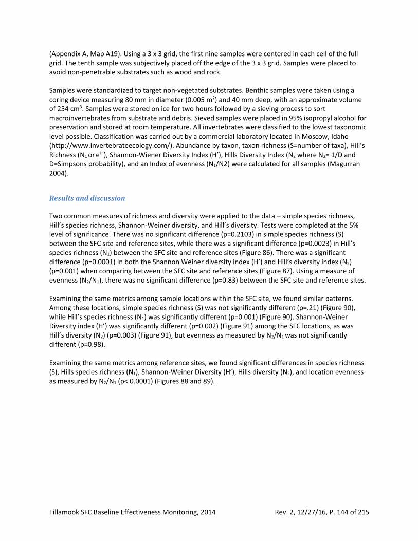
Tillamook SFC Baseline Effectiveness Monitoring, 2014 Rev. 2, 12/27/16, P. 144 of 215
(Appendix A, Map A19). Using a 3 x 3 grid, the first nine samples were centered in each cell of the full grid. The tenth sample was subjectively placed off the edge of the 3 x 3 grid. Samples were placed to avoid non-penetrable substrates such as wood and rock. Samples were standardized to target non-vegetated substrates. Benthic samples were taken using a coring device measuring 80 mm in diameter (0.005 m2) and 40 mm deep, with an approximate volume of 254 cm3. Samples were stored on ice for two hours followed by a sieving process to sort macroinvertebrates from substrate and debris. Sieved samples were placed in 95% isopropyl alcohol for preservation and stored at room temperature. All invertebrates were classified to the lowest taxonomic level possible. Classification was carried out by a commercial laboratory located in Moscow, Idaho (http://www.invertebrateecology.com/). Abundance by taxon, taxon richness (S=number of taxa), Hill’s Richness (N1 or eH’), Shannon-Wiener Diversity Index (H’), Hills Diversity Index (N2 where N2= 1/D and D=Simpsons probability), and an Index of evenness (N1/N2) were calculated for all samples (Magurran 2004).
Results and discussion Two common measures of richness and diversity were applied to the data – simple species richness, Hill’s species richness, Shannon-Weiner diversity, and Hill’s diversity. Tests were completed at the 5% level of significance. There was no significant difference (p=0.2103) in simple species richness (S) between the SFC site and reference sites, while there was a significant difference (p=0.0023) in Hill’s species richness (N1) between the SFC site and reference sites (Figure 86). There was a significant difference (p=0.0001) in both the Shannon Weiner diversity index (H’) and Hill’s diversity index (N2) (p=0.001) when comparing between the SFC site and reference sites (Figure 87). Using a measure of evenness (N2/N1), there was no significant difference (p=0.83) between the SFC site and reference sites. Examining the same metrics among sample locations within the SFC site, we found similar patterns. Among these locations, simple species richness (S) was not significantly different (p=.21) (Figure 90), while Hill’s species richness (N1) was significantly different (p=0.001) (Figure 90). Shannon-Weiner Diversity index (H’) was significantly different (p=0.002) (Figure 91) among the SFC locations, as was Hill’s diversity (N2) (p=0.003) (Figure 91), but evenness as measured by N2/N1 was not significantly different (p=0.98). Examining the same metrics among reference sites, we found significant differences in species richness (S), Hills species richness (N1), Shannon-Weiner Diversity (H’), Hills diversity (N2), and location evenness as measured by N2/N1 (p< 0.0001) (Figures 88 and 89).
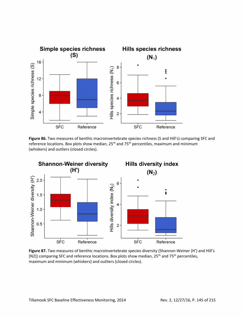
Tillamook SFC Baseline Effectiveness Monitoring, 2014 Rev. 2, 12/27/16, P. 145 of 215
Figure 86. Two measures of benthic macroinvertebrate species richness (S and Hill’s) comparing SFC and reference locations. Box plots show median, 25th and 75th percentiles, maximum and minimum (whiskers) and outliers (closed circles).
Figure 87. Two measures of benthic macroinvertebrate species diversity (Shannon-Weiner (H’) and Hill’s [N2]) comparing SFC and reference locations. Box plots show median, 25th and 75th percentiles, maximum and minimum (whiskers) and outliers (closed circles).
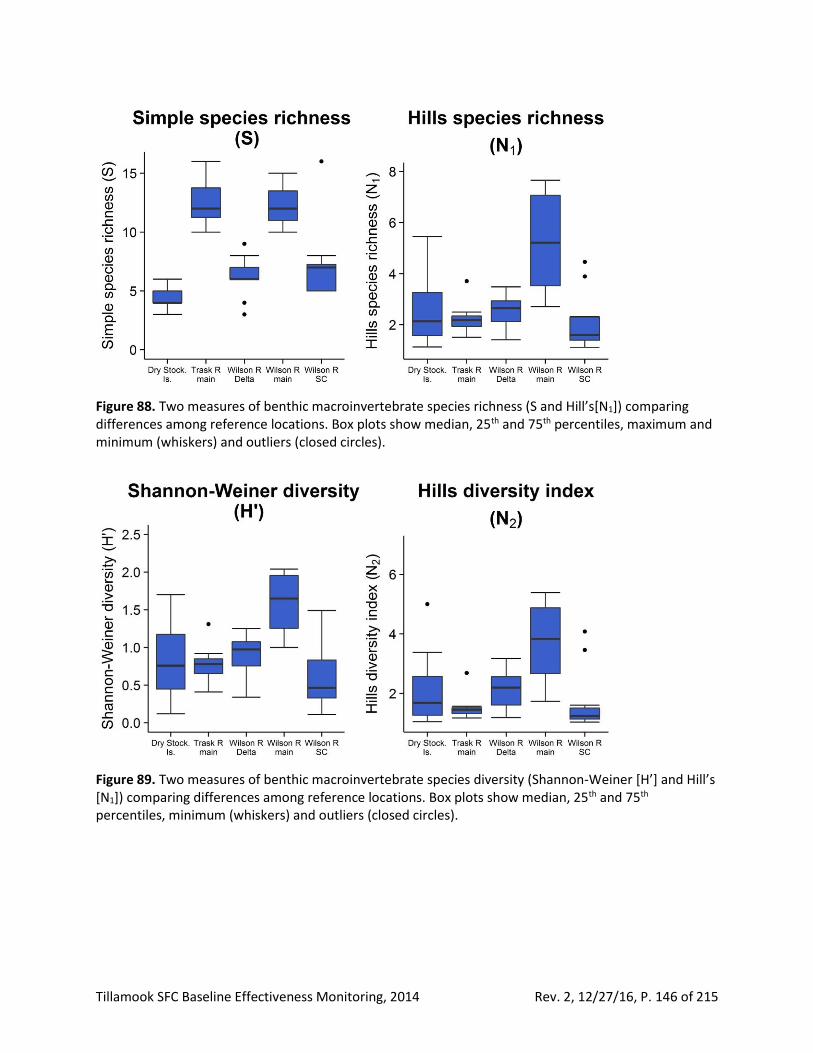
Tillamook SFC Baseline Effectiveness Monitoring, 2014 Rev. 2, 12/27/16, P. 146 of 215
Figure 88. Two measures of benthic macroinvertebrate species richness (S and Hill’s[N1]) comparing differences among reference locations. Box plots show median, 25th and 75th percentiles, maximum and minimum (whiskers) and outliers (closed circles).
Figure 89. Two measures of benthic macroinvertebrate species diversity (Shannon-Weiner [H’] and Hill’s [N1]) comparing differences among reference locations. Box plots show median, 25th and 75th percentiles, minimum (whiskers) and outliers (closed circles).
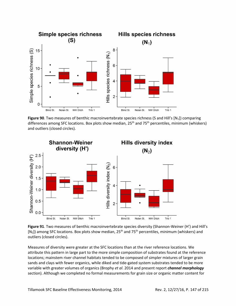
Tillamook SFC Baseline Effectiveness Monitoring, 2014 Rev. 2, 12/27/16, P. 147 of 215
Figure 90. Two measures of benthic macroinvertebrate species richness (S and Hill’s [N1]) comparing differences among SFC locations. Box plots show median, 25th and 75th percentiles, minimum (whiskers) and outliers (closed circles).
Figure 91. Two measures of benthic macroinvertebrate species diversity (Shannon-Weiner (H’) and Hill’s [N2]) among SFC locations. Box plots show median, 25th and 75th percentiles, minimum (whiskers) and outliers (closed circles). Measures of diversity were greater at the SFC locations than at the river reference locations. We attribute this pattern in large part to the more simple composition of substrates found at the reference locations; mainstem river channel habitats tended to be composed of simpler mixtures of larger grain sands and clays with fewer organics, while diked and tide-gated system substrates tended to be more variable with greater volumes of organics (Brophy et al. 2014 and present report channel morphology section). Although we completed no formal measurements for grain size or organic matter content for

Tillamook SFC Baseline Effectiveness Monitoring, 2014 Rev. 2, 12/27/16, P. 148 of 215
the substrates sampled, it was readily apparent to the observer that the large volume of large-grain sands remaining in the samples after sieving was completed was much greater at the reference locations compared to those from the SFC locations. In addition, the sieving process provided the sampler an opportunity to observe the volume of fine organic material flushed through the sieve during the washing process. Nanami et al. (2005) and Degraer (2008) have shown that grain size and sediment type affect estuarine benthic macroinvertebrate community structure. Additionally, we observed greater diversity in benthic communities in Coquille River Estuary high marsh channels as a result of greater substrate complexity, organic content, and seasonal salinity profiles (Brophy et al. 2014). Our single high marsh reference channel (DSI) did not have these characteristics, which likely relates to its less diverse benthic community, more similar to that of a mainstem river channel. Summed multispecies abundance values were higher in the reference locations when compared to the SFC locations (Appendix C, Table C8). Four of the five reference locations were dominated by amphipods and copepods (both crustaceans), while the fifth was dominated by chironomids (midges). Chironomids, oligochaetes (annelids), and hydrobiidae (mud snails) were dominant within the SFC locations (Appendix C, Table C10). These taxa are known to be associated with substrates with high levels of organic material (Day et al. 1989, Levington 1989, Delince 1992). Amphipods, or copepods, were also present in relatively high numbers at two of the SFC locations (Appendix C, Table C8). In summary, our SFC benthic macroinvertebrate community was similar to those observed in other Oregon estuarine wetlands (Brophy et al. 2014) where 1) dikes and tide gates resulted in limited tidal exchange, lower salinity, and finer-grained substrates with higher organic content; and 2) those substrates found in the reference locations were larger grained with less organic matter. As an exception to what we have observed in other Oregon diked tidal wetlands is the presences of the New Zealand mudsnail (Potamopyrgus antipodarum). This species became established in the lower Columbia River, Washington, about 1999 (http://nas.er.usgs.gov/queries/factsheet.aspx?SpeciesID=1008). The snail is described as tolerating siltation, thriving in disturbed watersheds, and benefiting from high nutrient flows that allow for filamentous green algae growth. It occurs among macrophytes and prefers littoral zones in lakes or slow streams with silt and organic matter substrates (Collier et al. 1998, Death et al. 2003, Holomuzki and Biggs 1999, Holomuzki and Biggs 2000, Weatherhead and James 2001, Zaranko et al. 1997). This species is euryhaline, establishing populations in fresh and brackish water. The optimal salinity has been suggested to be near or below 5 PSU, but the mudsnail is capable of feeding, growing, and reproducing at salinities of 0 – 15 PSU, and can tolerate salinities of 30 – 35 PSU for short periods of time (Costil et al. 2001, Gerard et al. 2003). Based on this information, and the presence of this species at a single SFC location and lack of presence at reference locations, we suggest there is the predicted increased salinities, tidal flushing, and shift in channel sediments and algal communities will result in the elimination of this species with the SFC site, or a reduced expansion of the species post-restoration. As described in Channel morphology above, when tidal forces are introduced to the SFC site following construction of the project, we expect to see morphological shifts towards equilibrium resulting in scour and fill of existing channel habitats. We expect to see significant scour of the fine sediments currently present in the SFC channels, as well as a shift in algal communities. Scour will likely occur in the form of large head cuts beginning where tide gates have been removed, and will work upstream over time. As scour occurs, fill will also occur initially in the form of shallow bars and along the banks as the channel meander forms and equilibrates. This initial scour and fill pattern will likely have a significant effect on benthic macroinvertebrate communities. Increased salinities will also likely greatly affect community structure. Based on summer salinity profiles at the reference locations, we expect the NW Ditch and Nolan Slough to be more saline than Blind Slough. In the near term (5 yrs), we expect the SFC benthic macroinvertebrate community to become more like that of the reference locations with less diversity
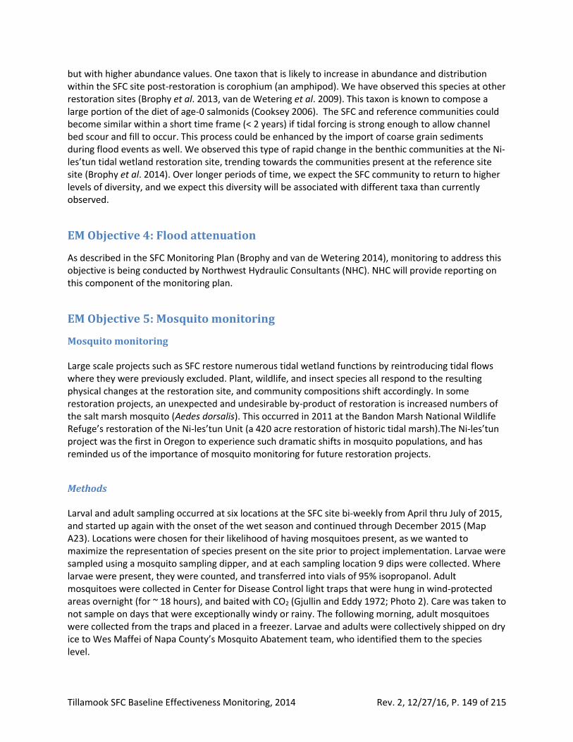
Tillamook SFC Baseline Effectiveness Monitoring, 2014 Rev. 2, 12/27/16, P. 149 of 215
but with higher abundance values. One taxon that is likely to increase in abundance and distribution within the SFC site post-restoration is corophium (an amphipod). We have observed this species at other restoration sites (Brophy et al. 2013, van de Wetering et al. 2009). This taxon is known to compose a large portion of the diet of age-0 salmonids (Cooksey 2006). The SFC and reference communities could become similar within a short time frame (< 2 years) if tidal forcing is strong enough to allow channel bed scour and fill to occur. This process could be enhanced by the import of coarse grain sediments during flood events as well. We observed this type of rapid change in the benthic communities at the Ni-les’tun tidal wetland restoration site, trending towards the communities present at the reference site site (Brophy et al. 2014). Over longer periods of time, we expect the SFC community to return to higher levels of diversity, and we expect this diversity will be associated with different taxa than currently observed.
EM Objective 4: Flood attenuation
As described in the SFC Monitoring Plan (Brophy and van de Wetering 2014), monitoring to address this objective is being conducted by Northwest Hydraulic Consultants (NHC). NHC will provide reporting on this component of the monitoring plan.
EM Objective 5: Mosquito monitoring
Mosquito monitoring Large scale projects such as SFC restore numerous tidal wetland functions by reintroducing tidal flows where they were previously excluded. Plant, wildlife, and insect species all respond to the resulting physical changes at the restoration site, and community compositions shift accordingly. In some restoration projects, an unexpected and undesirable by-product of restoration is increased numbers of the salt marsh mosquito (Aedes dorsalis). This occurred in 2011 at the Bandon Marsh National Wildlife Refuge’s restoration of the Ni-les’tun Unit (a 420 acre restoration of historic tidal marsh).The Ni-les’tun project was the first in Oregon to experience such dramatic shifts in mosquito populations, and has reminded us of the importance of mosquito monitoring for future restoration projects.
Methods Larval and adult sampling occurred at six locations at the SFC site bi-weekly from April thru July of 2015, and started up again with the onset of the wet season and continued through December 2015 (Map A23). Locations were chosen for their likelihood of having mosquitoes present, as we wanted to maximize the representation of species present on the site prior to project implementation. Larvae were sampled using a mosquito sampling dipper, and at each sampling location 9 dips were collected. Where larvae were present, they were counted, and transferred into vials of 95% isopropanol. Adult mosquitoes were collected in Center for Disease Control light traps that were hung in wind-protected areas overnight (for ~ 18 hours), and baited with CO2 (Gjullin and Eddy 1972; Photo 2). Care was taken to not sample on days that were exceptionally windy or rainy. The following morning, adult mosquitoes were collected from the traps and placed in a freezer. Larvae and adults were collectively shipped on dry ice to Wes Maffei of Napa County’s Mosquito Abatement team, who identified them to the species level.
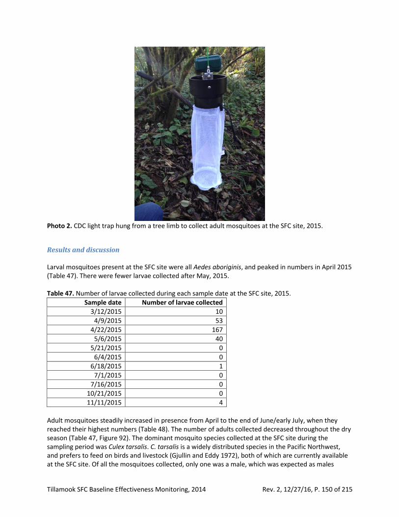
Tillamook SFC Baseline Effectiveness Monitoring, 2014 Rev. 2, 12/27/16, P. 150 of 215
Photo 2. CDC light trap hung from a tree limb to collect adult mosquitoes at the SFC site, 2015.
Results and discussion Larval mosquitoes present at the SFC site were all Aedes aboriginis, and peaked in numbers in April 2015 (Table 47). There were fewer larvae collected after May, 2015. Table 47. Number of larvae collected during each sample date at the SFC site, 2015.
Sample date Number of larvae collected
3/12/2015 10
4/9/2015 53
4/22/2015 167
5/6/2015 40
5/21/2015 0
6/4/2015 0
6/18/2015 1
7/1/2015 0
7/16/2015 0
10/21/2015 0
11/11/2015 4
Adult mosquitoes steadily increased in presence from April to the end of June/early July, when they reached their highest numbers (Table 48). The number of adults collected decreased throughout the dry season (Table 47, Figure 92). The dominant mosquito species collected at the SFC site during the sampling period was Culex tarsalis. C. tarsalis is a widely distributed species in the Pacific Northwest, and prefers to feed on birds and livestock (Gjullin and Eddy 1972), both of which are currently available at the SFC site. Of all the mosquitoes collected, only one was a male, which was expected as males
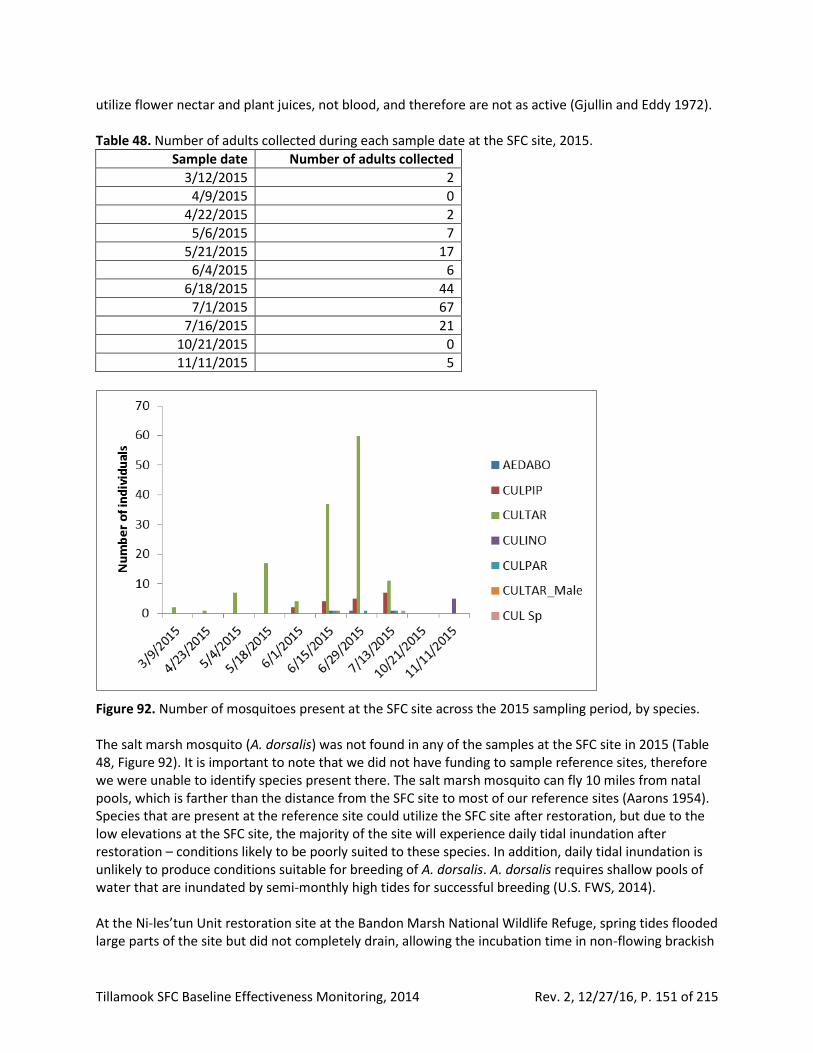
Tillamook SFC Baseline Effectiveness Monitoring, 2014 Rev. 2, 12/27/16, P. 151 of 215
utilize flower nectar and plant juices, not blood, and therefore are not as active (Gjullin and Eddy 1972). Table 48. Number of adults collected during each sample date at the SFC site, 2015.
Sample date Number of adults collected
3/12/2015 2
4/9/2015 0
4/22/2015 2
5/6/2015 7
5/21/2015 17
6/4/2015 6
6/18/2015 44
7/1/2015 67
7/16/2015 21
10/21/2015 0
11/11/2015 5
Figure 92. Number of mosquitoes present at the SFC site across the 2015 sampling period, by species. The salt marsh mosquito (A. dorsalis) was not found in any of the samples at the SFC site in 2015 (Table 48, Figure 92). It is important to note that we did not have funding to sample reference sites, therefore we were unable to identify species present there. The salt marsh mosquito can fly 10 miles from natal pools, which is farther than the distance from the SFC site to most of our reference sites (Aarons 1954). Species that are present at the reference site could utilize the SFC site after restoration, but due to the low elevations at the SFC site, the majority of the site will experience daily tidal inundation after restoration – conditions likely to be poorly suited to these species. In addition, daily tidal inundation is unlikely to produce conditions suitable for breeding of A. dorsalis. A. dorsalis requires shallow pools of water that are inundated by semi-monthly high tides for successful breeding (U.S. FWS, 2014). At the Ni-les’tun Unit restoration site at the Bandon Marsh National Wildlife Refuge, spring tides flooded large parts of the site but did not completely drain, allowing the incubation time in non-flowing brackish
Tillamook SFC Baseline Effectiveness Monitoring, 2014 Rev. 2, 12/27/16, P. 152 of 215
water needed by A. dorsalis larvae. Small first-order channels were underrepresented in the excavated channel network at the Ni-les’tun Unit. Therefore, small pools formed in locally-subsided micro-topographic depressions on the marsh surface. To address this problem, the U.S. FWS excavated an additional 40,000 linear feet of first- and second-order tidal channels to eliminate the mosquito-breeding habitat using hand-shovel crews and machinery. The experience of U.S. FWS at Ni-les’tun provides an important lesson learned that can help guide channel design at the SFC site – namely, excavate channels in a way that avoids ponding. Table 49. Complete list of species found during 2014 mosquito monitoring at the SFC site.
Scientific name Species code
Aedes aboriginis AEDABO
Culex pipiens CULPIP
Culex tarsalis CULTAR
Culiseta inornata CULINO
Culiseta particeps CULPAR
Culex stigmatosoma CULSTI
CONCLUSIONS AND RECOMMENDATIONS Baseline monitoring showed striking differences between the SFC site and the reference sites. These differences are summarized in Key findings at the beginning of this report. During post-project monitoring, baseline conditions will be compared to conditions following project implementation to evaluate the project’s effectiveness in meeting its stated goals, as outlined in the SFC Effectiveness Monitoring Plan (Brophy and van de Wetering 2014). Post-project effectiveness monitoring should follow the recommendations and methods presented in the SFC Effectiveness Monitoring Plan (“EM Plan) (Brophy and van de Wetering 2014). The methods in the EM Plan were used for the baseline study documented in this report; continuation of the same methods will allow comparisons that are necessary for determination of project effectiveness. In addition, post-implementation monitoring should address performance criteria, as recommended in the project’s Environmental Impact Statement (http://southernfloweis.org/). Mosquito monitoring was not included in the EM Plan, but is an important component of project evaluation. West Coast mosquito expert Wes Maffei provided technical advice to our team during baseline mosquito monitoring at SFC; he recommends mosquito monitoring during Year 1 and Year 2 after project implementation. During project implementation, monitoring infrastructure (particularly accretion plots and groundwater wells) should be protected from damage and disturbance. If accretion plots are disturbed, comparisons of accretion rates before and after project implementation will not be possible. This study provided a variety of data to support restoration design and project planning at the SFC site and other projects in Oregon and the Pacific Northwest. Our team has made heavy use of the baseline monitoring data when providing input to project design, plans and other project documents. For the SFC project, examples include our team’s contributions to the SFC Baseline Documentation Report prepared for the Oregon Watershed Enhancement Board (OWEB) (Brown and Brophy 2015a; Paulus et al. 2016), recommendations for fish salvage provided in van de Wetering et al. (2014), and participation in formal

Tillamook SFC Baseline Effectiveness Monitoring, 2014 Rev. 2, 12/27/16, P. 153 of 215
and informal design review meetings and phone calls. Beyond this specific project, our team is making use of the SFC monitoring results to improve monitoring methods, restoration design, and evaluation of restoration effectiveness at numerous other projects. For example, we have used SFC baseline monitoring results to provide technical guidance for projects such as the Waite Ranch project in the Siuslaw River estuary, the Kilchis tidal wetland restoration project in the Tillamook Bay estuary, and the Wallooskee-Youngs tidal wetland restoration in the Columbia River estuary. Results of the blue carbon study at the SFC site and reference sites will form a major contribution to a Pacific Northwest blue carbon dataset being compiled by the Blue Carbon Working Group (of which Laura Brophy and Craig Cornu are members). Our SFC project monitoring results are and will continue to be disseminated to the restoration practitioner community and the scientific community through daily informal contacts in our large network of estuary practitioners and scientists, and through formal workshops, presentations and meetings.
Tillamook SFC Baseline Effectiveness Monitoring, 2014 Rev. 2, 12/27/16, P. 154 of 215
REFERENCES Aarons, T. 1954. Salt marsh mosquito survey in the San Francisco Bay area 1950-1953. Proc. C.M.C.A. 22:75-78.
Allen, J.R.L. 1990. Morphodynamics of Holocene salt marshes: a review sketch from the Atlantic and Sourthern North Sea coasts of Europe. Quaternary Science Reviews 19:1155-1231.
Bonham, C.D. 1989. Measurements for terrestrial vegetation. Wiley, New York.
Borde, A.B., V.I. Cullinan, H.L. Diefenderfer, R.M. Thom, R.M. Kaufmann, S.A. Zimmerman, J. Sagar, K.E. Buenau, and C. Corbett. 2011. Lower Columbia River and Estuary ecosystem restoration program reference site study: 2011 restoration analysis. PNNL-21433, Pacific Northwest National Laboratory, Richland, Washing.
Brophy, L.S. 2017. Annual Compensatory Wetland Mitigation Monitoring Report for 2016 (Year 9): Off-site Mitigation, North Fork Siuslaw River Bridge Project. Prepared for Siuslaw Soil and Water Conservation District and Oregon Department of Transportation. 27 pp. Green Point Consulting, Corvallis, OR.
Brophy, L.S. 2009. Effectiveness monitoring at tidal wetland restoration and reference sites in the Siuslaw River Estuary: a tidal swamp focus. Prepared for Ecotrust, Portland, Oregon. Green Point Consulting, Corvallis, Oregon. Accessed 2/28/16 at http://hdl.handle.net/1957/35621.
Brophy, L.S. 2007. Estuary Assessment: Component XII of the Oregon Watershed Assessment Manual. Report to the Oregon Department of Land Conservation and Development, Salem, OR and the Oregon Watershed Enhancement Board, Salem, OR. Green Point Consulting, Corvallis, Oregon. 134 pp. Accessed 10/29/13 at http://www.oregon.gov/OWEB/docs/pubs/wa_estuary/estuary_assessment_2007.pdf.
Brophy, L.S., C.E. Cornu, P.R. Adamus, J.A. Christy, A. Gray, M.A. MacClellan, J.A. Doumbia, and R.L. Tully. 2011. New tools for tidal wetland restoration: development of a reference conditions database and a temperature sensor method for detecting tidal inundation in least-disturbed tidal wetlands of Oregon, USA. Report to the Cooperative Institute for Coastal and Estuarine Environmental Technology (CICEET), Durham, NH. 199 pp. Accessed 2/28/16 at http://oregonexplorer.info/data_files/OE_topic/wetlands/documents/01_Brophy_Cornu_CICEET_FINAL_complete_30-Aug-2011.pdf.
Brophy, L.S. and C.N. Janousek. 2013. 2013 monitoring report: Pixieland tidal wetland restoration. Corvallis, Oregon: Green Point Consulting and the Estuary Technical Group, Institute for Applied Ecology.
Brophy, L.S., L.A. Brown, and M.J. Ewald. 2015. Waite Ranch baseline effectiveness monitoring: 2014. Corvallis, Oregon: Institute for Applied Ecology.
Brophy, L.S., and J. Lemmer. 2013. Waite Ranch interim management plan. Prepared for Oregon Watershed Enhancement Board. Green Point Consulting, Corvallis, OR, and McKenzie River Trust, Eugene, OR.
Tillamook SFC Baseline Effectiveness Monitoring, 2014 Rev. 2, 12/27/16, P. 155 of 215
Brophy, L.S. and S. van de Wetering. 2012. Ni-les’tun tidal wetland restoration effectiveness monitoring: baseline: 2010-2011. Corvallis, Oregon: Green Point Consulting, The Institute for Applied Ecology, and the Confederated Tribes of Siletz Indians. Accessed 8/13/12 at http://appliedeco.org/wp-content/uploads/Ni-lestun-Tidal-Wetland-Restoration-Effectiveness-Monitoring-Baseline-2010-2011.pdf.
Brophy, L.S., and S. van de Wetering. 2014. Southern Flow Corridor project effectiveness monitoring plan. Corvallis, OR: Institute for Applied Ecology and the Confederated Tribes of Siletz Indians. Accessed 7/25/14 at: http://ossfc.files.wordpress.com/2014/01/sfc_effectiveness_monitoring_plan_final_2014-01-07_rev1.pdf
Brophy, L.S., S. van de Wetering, M.J. Ewald, L.A. Brown, and C.N. Janousek. 2014. Ni-les’tun tidal wetland restoration effectiveness monitoring: Year 2 post-restoration (2013). Corvallis, Oregon: Institute for Applied Ecology.
Brown, L.A. and L.S. Brophy. 2015a. Invasive species list, maps and photo points for SFC Baseline Documentation Report. Memorandum to Wm. Fritz Paulus, 8/14/15. Estuary Technical Group, Institute for Applied Ecology, Corvallis, Oregon.
Brown, L.A. and L.S. Brophy. 2015b. 2015 monitoring report: Pixieland tidal wetland restoration. Corvallis, Oregon: Green Point Consulting and the Estuary Technical Group, Institute for Applied Ecology.
Brown, L.A., M.J. Ewald, and L.S. Brophy. 2015. Ni-les’tun tidal wetland restoration effectiveness monitoring: Year 4 post-restoration (2015). Corvallis, Oregon: Estuary Technical Group, Institute for Applied Ecology.
Cahoon, D.R., J.C. Lynch, and R.M. Knaus. 1996. Improved cryogenic coring device for sampling wetland soils. Journal of Sedimentary Research 66:1025-1027.
Cahoon, D.R., P.E. Marin, B.K. Black, and J.C. Lynch. 2000. A method for measuring vertical accretion elevation, and compaction of soft, shallow-water sediments. Journal of Sedimentary Research 70:1250-1253.
Cahoon, D.R., P.F. Hensel, T. Spencer, D.J. Reed, K.L. McKee, and N. Saintilan. 2006. Coastal wetland vulnerability to relative sea-level rise: wetland elevation trends and process controls. In: Verhoeven, J.T.A., B. Beltman, R. Bobbink, and D. Whigham (Eds.), Wetlands and Natural Resource Management. Ecological Studies, vol. 190. Springer-Verlag, Berlin/Heidelberg, pp.271-292.
Cahoon, D.R. and R.E. Turner. 1989. Accretion and canal impacts in a rapidly subsiding wetland II. Feldspar marker horizon technique. Estuaries 12:260-268.
Coats, R.N., P.B. Williams, C.K. Cuffe, J. Zedler, D. Reed, S. Watry and J. Noller. 1995. Design guidelines for tidal channels in coastal wetlands. Report prepared for the U.S. Army Corps of Engineers Waterways Experiment Station, Vicksburg, MS. Philip Williams and Assoc., Ltd. San Francisco, CA. 46 pp.
Collier, K.J., R.J. Wilcock, and A.S. Meredith. 1998. Influence of substrate type and physico-chemical conditions on macroinvertebrate faunas and biotic indices in some lowland Waikato, New Zealand, streams. New Zealand Journal of Marine and Freshwater Research 32:1-19.
Cook, T., S.C. Meyers, and S. Sundberg (Eds). 2013. Oregon Vascular Plant Checklist. http://www.oregonflora.org/checklist.php. Version 1.I4. Accessed 11/1/15.

Tillamook SFC Baseline Effectiveness Monitoring, 2014 Rev. 2, 12/27/16, P. 156 of 215
Cooksey, M.J. 2006. Fish community use of created intertidal habitats in an urban estuary: abundance patterns and diet composition of common estuarine fishes in the Lower Duwamis Waterway, Seattle, Washington. M.S. Thesis. University of Washington, Washington, USA.
Costil, K., G.B.J. Dussart, and J. Daquzan. 2001. Biodiversity of aquatic gastropods in the Mont St-Michael basin (France) in relation to salinity and drying of habitats. Biodiversity and Conservation 10:1-18.
Coulton, K., P.B. Williams, and P.A. Benner. 1996. An environmental history of the Tillamook Bay Estuary and watershed. Philip Williams and Associated, Ltd. Research Report CE 990292-1, Tillamook Bay National Estuary Project, Garibaldi, OR.
Craft, C.B., E.D. Seneca, and S.W. Broome. 1991. Loss on ignition and Kjeldahl digestion for estimating organic carbon and total nitrogen in estuarine marsh soils: calibration with dry combustion. Estuaries 14:175-179.
Day, J.W., Jr., C.A.S. Hall, W.M. Kemp, and A. Yáñez-Arancibia (Eds.). 1989. Estuarine ecology. John Wiley and Sons, Inc.
Death, R.G., B. Baillie, and P. Fransen. 2003. Effect of Pinus radiata logging on stream invertebrate communities in Hawke’s Bay, New Zealand. New Zealand Journal of Marine and Freshwater Research 37:507-520.
Degraer, S., E. Verfaillie, W. Willems, E. Adriaens, M. Vincx, and V. Van Lancker. 2008. Habitat suitability modelling as a mapping tool for macrobenthic communities: An example from the Belgian part of the North Sea. Continental Shelf Research, 28(3):369-379. doi: 10.1016/j.csr.2007.09.001.
Delince, G. 1992. The ecology of the fish pond ecosystem. Springer Science Business Media B.V.
Dicken, S.N. 1961. Some recent physical changes of the Oregon coast. Report for the Office of Naval Research, U.S. Department of the Navy, Contract Nonr-2771(04). Department of Geography, University of Oregon.
Diefenderfer, H.L., A.M. Coleman, A.B. Borde, and I.A. Sinks. 2008. Hydraulic geometry and microtopography of tidal freshwater forested wetlands and implications for restoration, Columbia River, U.S.A International Journal of Ecohydrology and Hydrobiology 8(2-4):339-361.
Environmental Laboratory. 1987. Corps of Engineers Wetlands Delineation Manual. Technical report Y-87-1, U.S. Army Engineer Waterways Experiment Station, Vicksburg, MS.
Ewald, M.J. and L.S. Brophy. 2012. Tidal wetland prioritization for the Tillamook Bay estuary. Prepared for the Tillamook Estuaries Partnership, Garibaldi, OR. Estuary Technical Group of the Institute for Applied Ecology and Green Point Consulting, Corvallis, OR. Accessed 9/29/15 at http://www.wildsalmon center.org/pdf/TillamookWetlandsReport-FINAL.pdf.
Frenkel, R. E. and J.C. Morlan. 1991. Can we restore our salt marshes? Lessons from the Salmon River, Oregon. The Northwest Environmental Journal 7:119-135.
Fofonoff, N.P. and R.C. Millard Jr. 1983. Algorithms for computation of fundamental properties of seawater. UNESCO Technical Papers in Marine Science No. 44. http://unesdoc.unesco.org/images/0005/000598/059832eb.pdf
Tillamook SFC Baseline Effectiveness Monitoring, 2014 Rev. 2, 12/27/16, P. 157 of 215
Gerard, C., A. Blanc, and K. Costil. 2003. Potamopyrgus antipodarum (Mollusca: Hydrobiidae) in continental aquatic gastropod communities: impacts of salinity and trematode parasitism. Hydrobiologica 493:167-172.
Gjullin, C.M. and G.W. Eddy. 1972. The mosquitoes of the Northwestern United States. Technical Bulletin No. 1447. Agricultural Research Service, United States Department of Agriculture, Washington, D.C.
Gough, L., J.B. Grace, and K.L. Taylor. 1994. The relationship between species richness and community biomass: the importance of environmental variables. Oikos 70:271-279.
Grace, J.B., and B.H. Pugesek. 1997. A structural equation model of plant species richness and its application to a coastal wetland. American Naturalist 149:436-460.
Hawes, S.M., J.A. Hiebler, E.M. Nielsen, C.W. Alton, J.A. Christy, and P. Benner. 2008. Historical vegetation of the Pacific Coast, Oregon, 1855-1910. ArcMap shapefile, Version 2008_03. Oregon Natural Heritage Information Center, Oregon State University. http://www.pdx.edu/sites/www.pdx.edu.pnwlamp/files/glo_coast_2008_03.zip.
Holomuzki, J.R. and B.J.F. Biggs. 1999. Distributional responses to flow disturbance by a stream-dwelling snail. Oikos 87:36-47.
Holomuzki, J.R. and B.J.F. Biggs. 2000. Taxon-specific responses to high-flow disturbances in streams: implications for population persistence. Journal of the North American Benthological Society 19:670-679.
Hood, W.G. 2002. Application of landscape allometry to restoration of tidal channels. Restoration Ecology 10:213-222.
Hood, W.G. 2004. Indirect environmental effects of dikes on estuarine tidal channels: thinking outside of the dike for habitat restoration and monitoring. Estuaries 27:273-282.
Hood, W.G. 2007. Landscape allometry and prediction in estuarine and coastal ecology: linking landform scaling to ecological patterns and processes. Estuaries and Coasts 30:895-900.
Hood, W.G. 2014. Difference in tidal channel network geometry between reference marshes and marshes restored by historical dike breaching. Ecological Engineering 71:563-573.
Huang, L., L. Brophy, and C. Lindley. 2011. Fluvial effects on coastal flooding in the U.S. Pacific Northwest. Proceedings of Solutions to Coastal Disasters 2011, Anchorage, AK. 12 pp.
Janousek, C.N., and C.L. Folger. 2014. Variation in tidal wetland plant diversity and composition within and among coastal estuaries: Assessing the relative importance of environmental gradients. Journal of Vegetation Science 25: 534–545.
Jay, D.A., and T. Kukulka. 2003. Revising the paradigm of tidal analysis – the uses of non-stationary data. Ocean Dynamics 53(3): 110-125.
Kasozi, G.N., P. Nkedi-Kizza, and W.G. Harris. 2009. Varied carbon content of organic matter in histosols, spodosols, and carbonatic soils. Soil Science Society of America Journal 73:1313-1318.
Tillamook SFC Baseline Effectiveness Monitoring, 2014 Rev. 2, 12/27/16, P. 158 of 215
Kunza, A.E. and S.C. Pennings. 2008. Patterns of plant diversity in Georgia and Texas salt marshes. Estuaries and Coasts 31:673-681.
Levington, J.S 1989. Deposit feeding and coastal oceanography. In G. Lopez et al. (Eds.). 1989. Ecology of marine deposit feeders. Springer-Verlag New York, Inc.
MacClellan, M.A. 2012. Carbon content in Oregon tidal wetland soils. Master’s Project Research Report, Marine Resource Management Program, College of Oceanic and Atmospheric Sciences, Oregon State University, Corvallis, OR. 30pp. Accessed 10/16/15 at http://hdl.handle.net/1957/25502.
Magurran, A.E. 2004. Measuring biological diversity. Blackwell Science, Ltd. Blackwell publishing , 350 Main Street, Malden, MA 02148, USA.
Matte, P., D.A. Jay, and E.D. Zaron. 2013. Adaptation of classical tidal harmonic analysis to nonstationary tides, with application to river tides. Journal of Atmospheric and Oceanic Technology, 30(3), 569-589.
Maundera, M.N., J.R. Sibert, A. Fonteneau, J. Hampton, P. Keleiber, and S.J. Harley. 2006. Interpreting catch per unit effort data to assess the status of individual stocks and communities. ICES J. Mar. Sci. 63:1373-1385.
Nanami, A., H. Saito, T. Akita, K-I. Motomatsu, and H. Kuwahara. 2005. Spatial distribution and assemblage structure of macrobenthic invertebrates in a brackish lake in relation to environmental variables. Estuarine, Coastal and Shelf Science 63:167-176
National Oceanic and Atmospheric Administration. Climatological Rankings, accessed 10/27/15. https://www.ncdc.noaa.gov/temp-and-precip/climatological-rankings/.
National Oceanic and Atmospheric Administration National Ocean Service (NOAA/NOS). 2003. Computational techniques for tidal datums handbook. NOAA Special Publication NOS CO-OPS 2. NOAA, National Ocean Service (NOS), Center for Operational Oceanographic Products and Services (COOPS). Silver Springs, Maryland, Accessed 5/31/14 at https://tidesandcurrents.noaa.gov/publications/Computational_Techniques_for_Tidal_Datums_handbook.pdf.
NHC (Northwest Hydraulic Consultants, Inc.). 2011. Southern Flow Corridor Landowner Preferred Alternative Preliminary Design Report. Prepared for Oregon Solutions Design Team under contract to Tillamook County. NHC Inc., Seattle, WA.
Parametrix. 2011. First annual wetland mitigation monitoring report: Goodspeed Road site. Report to Tillamook County. Parametrix, Portland, Oregon.
Paulus, W.F., with L. Brown, L. Brophy, V. Collins, and R. Hagerty on behalf of Tillamook County/Grantor. 2016. Baseline Inventory Documentation: Southern Flow Corridor Conservation Easement. Prepared for State of Oregon and Oregon Watershed Enhancement Board/Grantee.
Phillip Williams and Associates. 2002. Tillamook Bay integrated river management strategy. Report to U.S. Fish and Wildlife Service, U.S. Environmental Protection Agency, and U.S. Army Corps of Engineers. Phillip Williams and Associates, Corte Madera, CA.
R Core Team. 2014. R: a language and environmental for statistical computing. R Foundation for Statistical Computing, Vienna, Austria. URL http://www.R-project.org/.
Tillamook SFC Baseline Effectiveness Monitoring, 2014 Rev. 2, 12/27/16, P. 159 of 215
Rice, C.A., W.G. Hood, L.M. Tear, C.A. Simenstad, G.D. Williams, L.L. Johnson, B.E. Feist, and P. Roni. 2005. Monitoring rehabilitation in temperature North American estuaries. In P. Roni (Ed.), Methods for monitoring stream and watershed restoration. Am. Fisheries Soc., Bethesda, MD.
Roegner, G.C., H.L. Diefenderfer, A.B. Borde, R.M. Thom, E.M. Dawley, A.H. Whiting, S.A. Zimmerman, and G.E. Johnson. 2008. Protocols for monitoring habitat restoration projects in the lower Columbia River and estuary. PNNL-15793. Report by Pacific Northwest National Laboratory, National Marine Fisheries Service, and Columbia River Estuary Study Taskforce submitted to the U.S. Army Corps of Engineers, Portland District, Portland, Oregon.
Rosgen, D.L. 1994. A classification of natural rivers. Catena 22: 169-199
Rybczyk, J., T. Khangaonkar, G. Hood, and E. Reyes. 2011. Sustainable estuarine habitat restoration in the Pacific Northwest: modeling and managing the effects, feedbacks, and risks associated with climate change. Presented September 20, 2011 to the EPA.
Seliskar, D.M. and J.L. Gallagher. 1983. The ecology of tidal marshes in the Pacific Northwest coast: a community profile. U.S. Fish and Wildlife Service, Division of Biological Services, Washington, D.C. FWS/OBS-82/32. 65 pp.
Simenstad, C.A., C.D. Tanner, R.M. Thom, and L. Conquest. 1991. Estuarine Habitat Assessment Protocol. EPA 910/9-91-037, Puget Sound Estuary Program, U.S. Environ. Protect. Agency - Region 10, Seattle, WA. 191 pp + append.
Simenstad, C.A. and R.M. Thom. 1996. Functional equivalency trajectories of the restored Gog-Le-Hi-Te Estuarine Wetland. Ecological Applications 6:38.
So, K., S. van de Wetering, R. Van Hoy, and J. Mills. 2009. An analysis of reference tidal channel plan form characteristics for the Ni-les’tun Unit Restoration. February 2009 draft, US Fish and Wildlife Service, Confederated Tribes of Siletz Indians, Ducks Unlimited, and NOAA.
Sprecher, S.W. 2000. Installing monitoring wells/piezometers in wetlands. WRAP Technical Notes Collection (ERDC TN-WRAP-00-02), U.S. Army Engineer Research and Development Center, Vicksburg, MS. http://www.wes.army.mil/el/wrap/pdf/tnwrap00-2.pdf.
Stewart-Oaten, A., W.W. Murdoch, and K.R. Parker. 1986. Environmental impact assessment: “pseudoreplication” in time? Ecology 67:929-940.
Stewart-Oaten, A., J.R. Bench, and C.W. Osenberg. 1992. Assessing effects of unreplicated perturbations: no simple solutions. Ecology 73:1396-1404.
Sutherland, W. J. 2000. Monitoring. The Conservation Handbook: Research, Management and Policy. Wiley-Blackwell pp. 36–64.
Thayer, G.W., T.A. McTigue, R.J. Salz, D.H. Merkey, F.M. Burrows, and P.F. Gayaldo, (eds.). 2005. Science-based restoration monitoring of coastal habitats, Volume Two: tools for monitoring coastal habitats. NOAA Coastal Ocean Program Decision Analysis Series No. 23. NOAA National Centers for Coastal Ocean Science, Silver Spring, MD. 628 pp. plus appendices.
Thom, R.M. 1992. Accretion rates of low intertidal salt marshes in the Pacific Northwest. Wetlands 12:147-156.
Tillamook SFC Baseline Effectiveness Monitoring, 2014 Rev. 2, 12/27/16, P. 160 of 215
Thom, R.M., R. Zeigler, and A.B. Borde. 2002. Floristic development patterns in a restored Elk River estuarine marsh, Grays Harbor, Washington. Restoration Ecology 10:487-496.
Tillamook County. 2013. Southern Flow Corridor-landowner preferred alternative: FY 2013 coastal and marine habitat restoration project grant application.
Turner, R.E., E.M. Swenson, C.S. Milan, J.M. Lee, and T.A. Oswald. 2004. Below-ground biomass in healthy and impaired salt marshes. Ecological Research 19:29-35.
United States Fish and Wildlife Service (U.S. FWS). 2014. Draft plan and environmental assessment for mosquito control for Bandon Marsh National Wildlife Refuge. Bandon, Oregon: Bandon Marsh National Wildlife Refuge, U.S. Fish and Wildlife Service.
van de Wetering, S.J. 2014. Benthic macroinvertebrate sample size requirements. Ni’les-tun Unit. Bandon Marsh National Wildlife Refuge. Technical Report. Department of Natural Resources. Confederated Tribes of Siletz Indians. Siletz, OR 97380, USA.
van de Wetering, S., B. Fertig and I. Kentta. 2014. Southern Flow Corridor pre-restoration preliminary analysis covering spatial and temporal fish distributions. Prepared for Tillamook County. Confederated Tribes of Siletz Indians, Siletz, OR.
van de Wetering, S., R. French, A. Hall, B. Smith, and A. Gray. 2009. Fisheries restoration efficacy monitoring report for the Little Nestucca USFWS Coastal Refuge property. Prepared for Ducks Unlimited, Inc. Prepared by Confederated Tribes of Siletz Indians and Cramer Fish Sciences, Inc. Siletz, OR, USA
van de Wetering, S., R. French, D. Rollins, and B. Blundon. 2007. Oregon Tidal Salt Marshes and Juvenile Salmonid Use Patterns - Mining a Chinook Dominant Data Set for Coho Specific Patterns. American Fisheries Society, Oregon Chapter.
Weatherhead, M.A. and M.R. James. 2001. Distribution of macroinvertebrates in relation to physical and biological variables in the littoral zone of nine New Zealand lakes. Hydrobiologia 462:115-129.
Williams, P.B., M.K. Orr, and N.J. Garrity. 2002. Hydraulic geometry: a geomorphic design tool for tidal marsh channel evolution in wetland restoration projects. Restoration Ecology 10:577-590.
Wilson, L., P. Scoles, and L.S. Brophy. 1997. Bay City local wetland inventory. Technical report to City of Bay City, Oregon.
Zaranko, D.T., D.G. Farara, and F.G. Thompson. 1997. Another exotic mollusk in the Laurentian Great Lakes: the New Zealand native Potamopyrgus antipodarum (Gray 1843) (Gastropoda, Hydrobiidae).
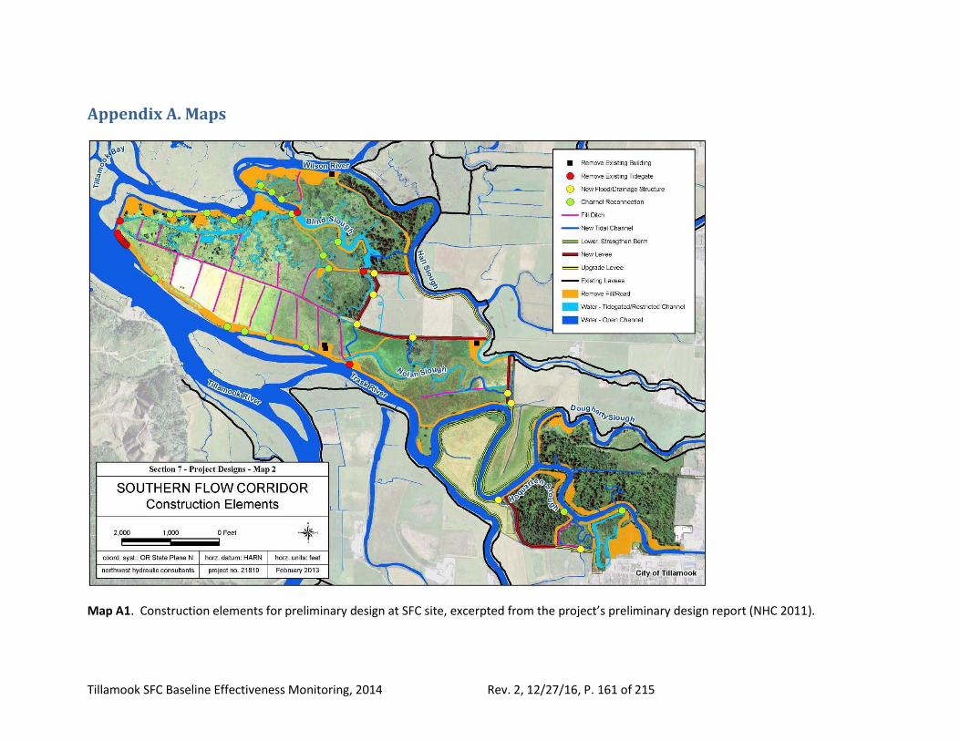
Tillamook SFC Baseline Effectiveness Monitoring, 2014 Rev. 2, 12/27/16, P. 161 of 215
Appendix A. Maps
Map A1. Construction elements for preliminary design at SFC site, excerpted from the project’s preliminary design report (NHC 2011).
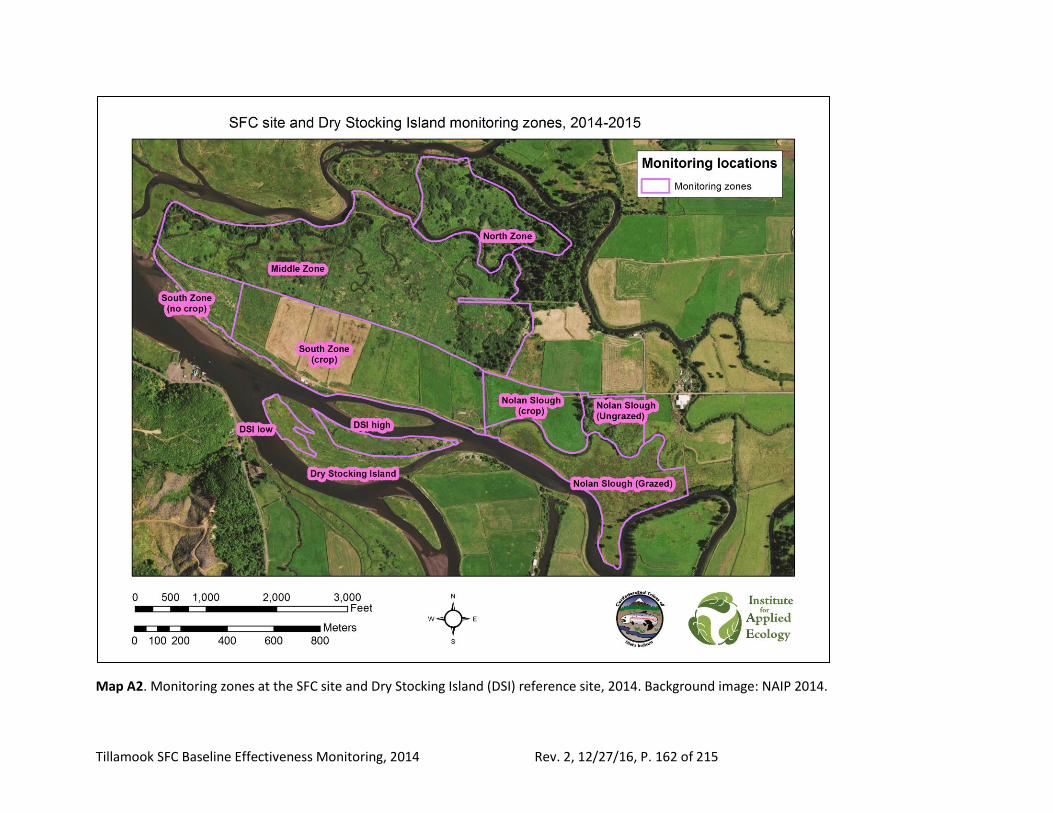
Tillamook SFC Baseline Effectiveness Monitoring, 2014 Rev. 2, 12/27/16, P. 162 of 215
Map A2. Monitoring zones at the SFC site and Dry Stocking Island (DSI) reference site, 2014. Background image: NAIP 2014.
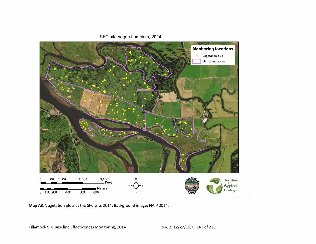
Tillamook SFC Baseline Effectiveness Monitoring, 2014 Rev. 2, 12/27/16, P. 163 of 215
Map A3. Vegetation plots at the SFC site, 2014. Background image: NAIP 2014.
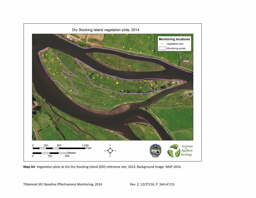
Tillamook SFC Baseline Effectiveness Monitoring, 2014 Rev. 2, 12/27/16, P. 164 of 215
Map A4. Vegetation plots at the Dry Stocking Island (DSI) reference site, 2014. Background image: NAIP 2014.
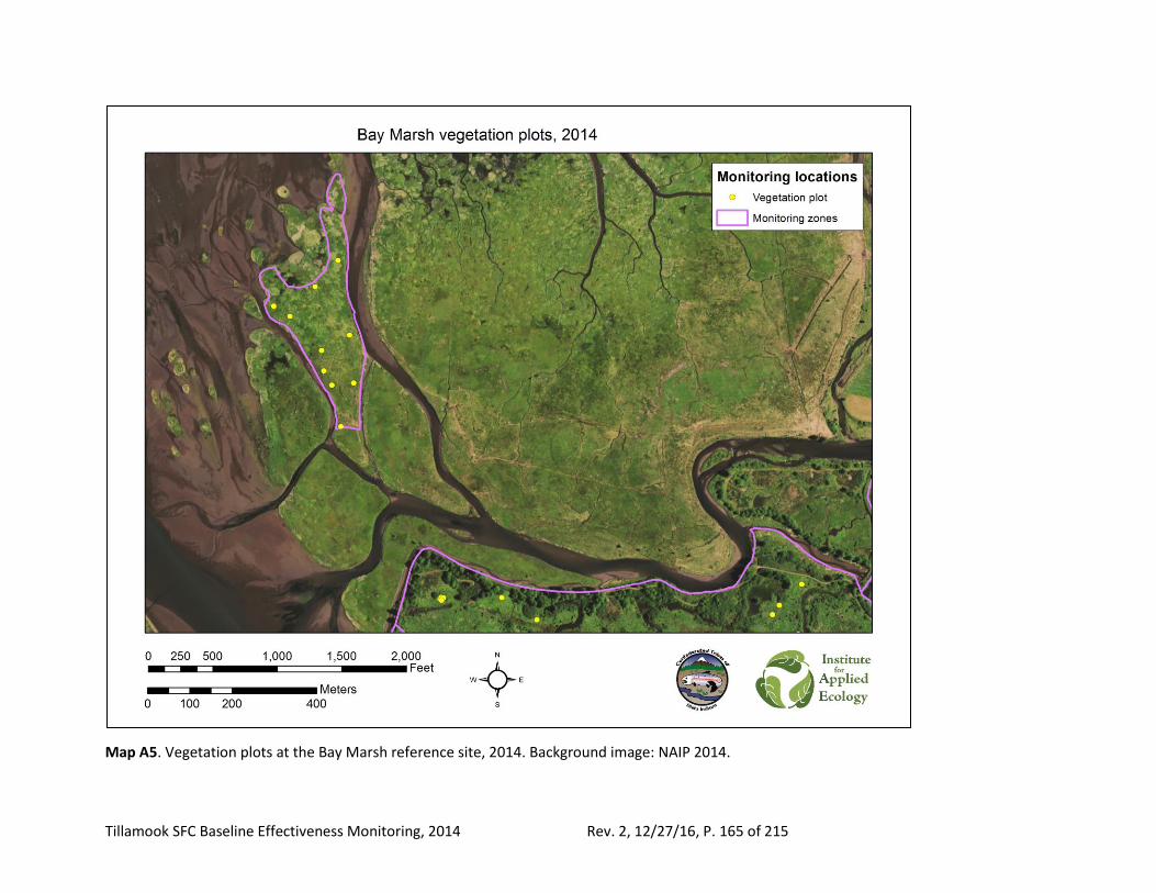
Tillamook SFC Baseline Effectiveness Monitoring, 2014 Rev. 2, 12/27/16, P. 165 of 215
Map A5. Vegetation plots at the Bay Marsh reference site, 2014. Background image: NAIP 2014.
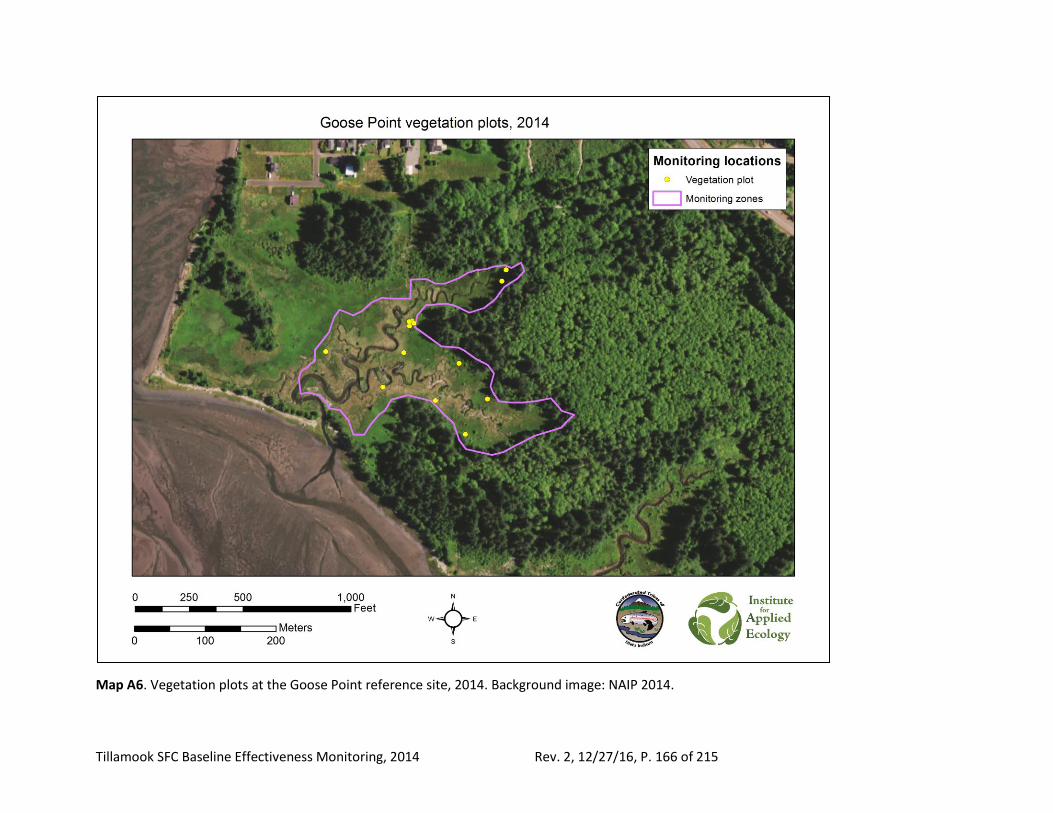
Tillamook SFC Baseline Effectiveness Monitoring, 2014 Rev. 2, 12/27/16, P. 166 of 215
Map A6. Vegetation plots at the Goose Point reference site, 2014. Background image: NAIP 2014.
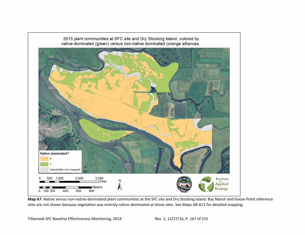
Tillamook SFC Baseline Effectiveness Monitoring, 2014 Rev. 2, 12/27/16, P. 167 of 215
Map A7. Native versus non-native dominated plant communities at the SFC site and Dry Stocking Island. Bay Marsh and Goose Point reference
sites are not shown because vegetation was entirely native-dominated at those sites. See Maps A8-A11 for detailed mapping.
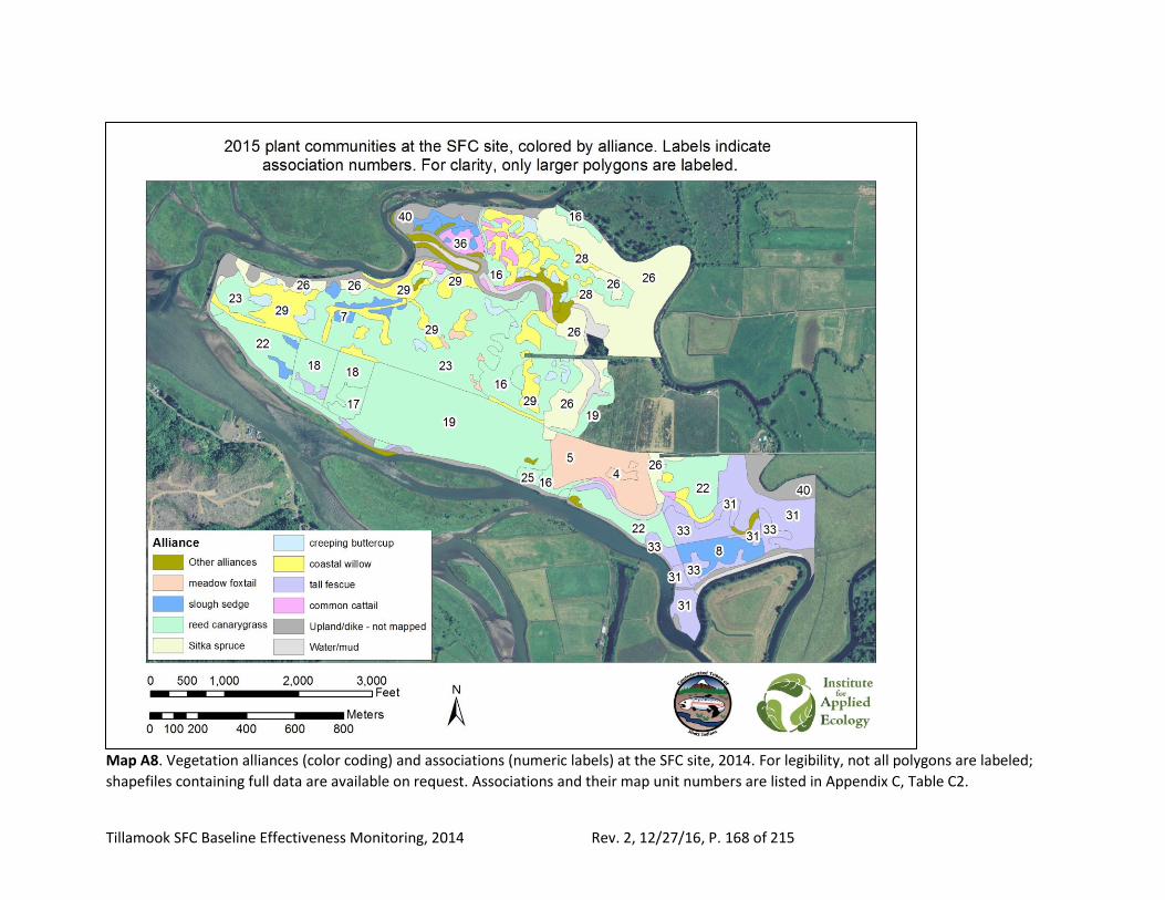
Tillamook SFC Baseline Effectiveness Monitoring, 2014 Rev. 2, 12/27/16, P. 168 of 215
Map A8. Vegetation alliances (color coding) and associations (numeric labels) at the SFC site, 2014. For legibility, not all polygons are labeled;
shapefiles containing full data are available on request. Associations and their map unit numbers are listed in Appendix C, Table C2.
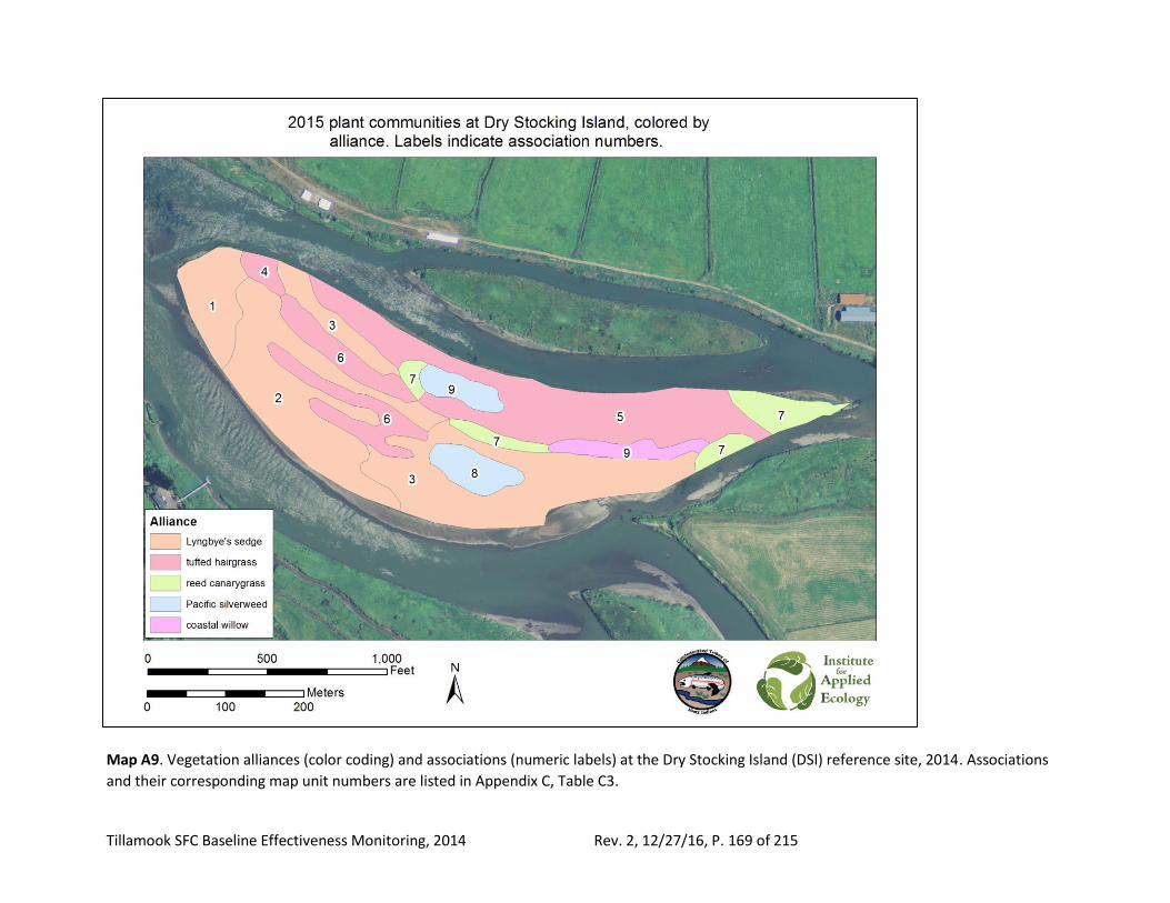
Tillamook SFC Baseline Effectiveness Monitoring, 2014 Rev. 2, 12/27/16, P. 169 of 215
Map A9. Vegetation alliances (color coding) and associations (numeric labels) at the Dry Stocking Island (DSI) reference site, 2014. Associations
and their corresponding map unit numbers are listed in Appendix C, Table C3.
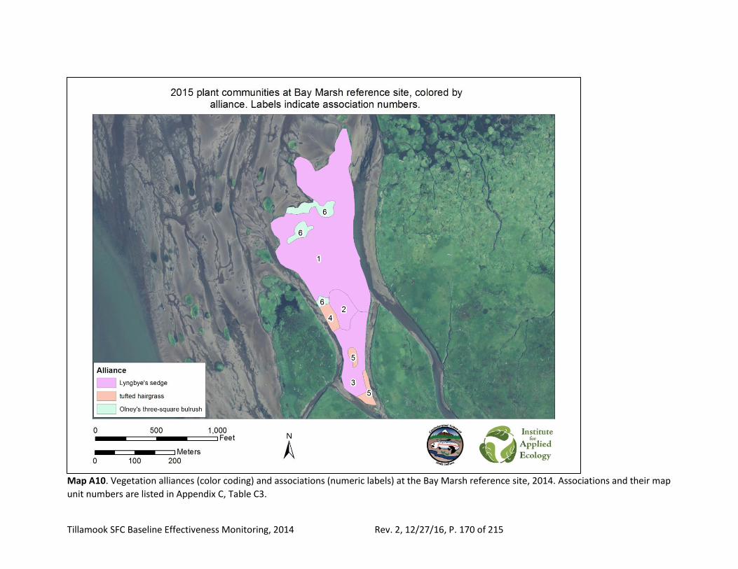
Tillamook SFC Baseline Effectiveness Monitoring, 2014 Rev. 2, 12/27/16, P. 170 of 215
Map A10. Vegetation alliances (color coding) and associations (numeric labels) at the Bay Marsh reference site, 2014. Associations and their map
unit numbers are listed in Appendix C, Table C3.
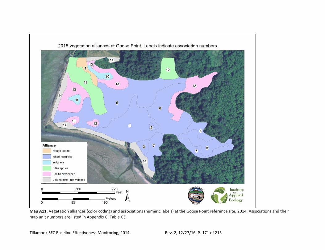
Tillamook SFC Baseline Effectiveness Monitoring, 2014 Rev. 2, 12/27/16, P. 171 of 215
Map A11. Vegetation alliances (color coding) and associations (numeric labels) at the Goose Point reference site, 2014. Associations and their
map unit numbers are listed in Appendix C, Table C3.
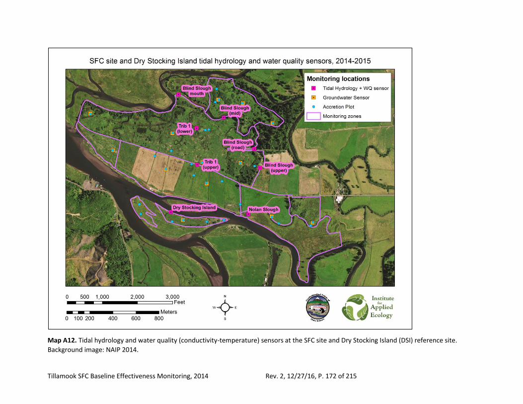
Tillamook SFC Baseline Effectiveness Monitoring, 2014 Rev. 2, 12/27/16, P. 172 of 215
Map A12. Tidal hydrology and water quality (conductivity-temperature) sensors at the SFC site and Dry Stocking Island (DSI) reference site.
Background image: NAIP 2014.
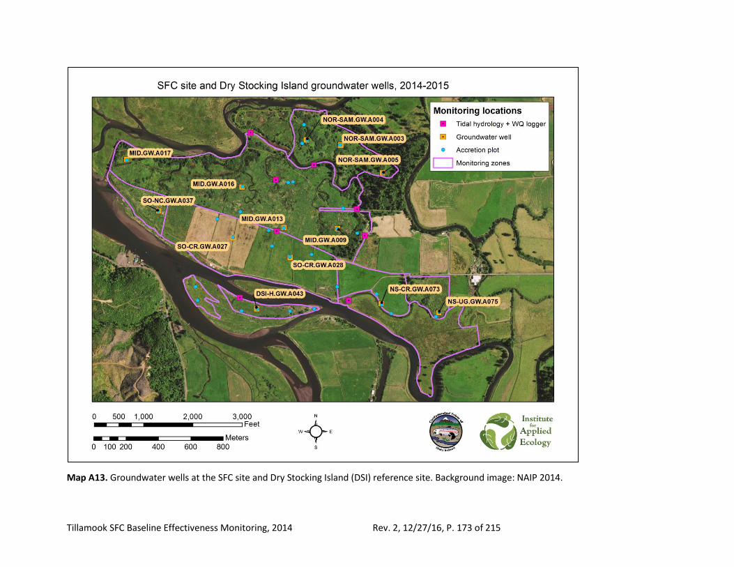
Tillamook SFC Baseline Effectiveness Monitoring, 2014 Rev. 2, 12/27/16, P. 173 of 215
Map A13. Groundwater wells at the SFC site and Dry Stocking Island (DSI) reference site. Background image: NAIP 2014.
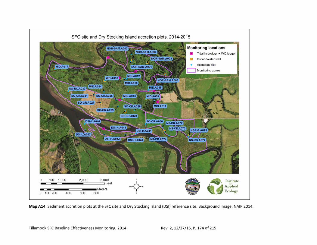
Tillamook SFC Baseline Effectiveness Monitoring, 2014 Rev. 2, 12/27/16, P. 174 of 215
Map A14. Sediment accretion plots at the SFC site and Dry Stocking Island (DSI) reference site. Background image: NAIP 2014.
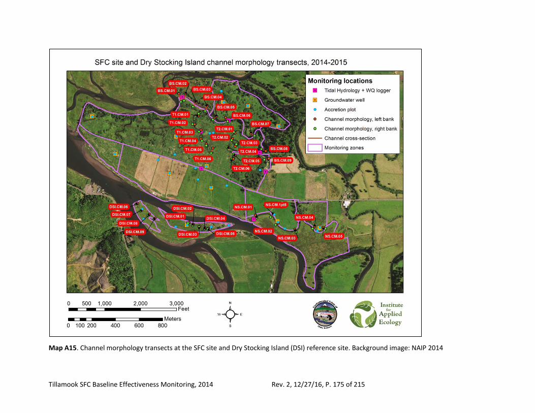
Tillamook SFC Baseline Effectiveness Monitoring, 2014 Rev. 2, 12/27/16, P. 175 of 215
Map A15. Channel morphology transects at the SFC site and Dry Stocking Island (DSI) reference site. Background image: NAIP 2014
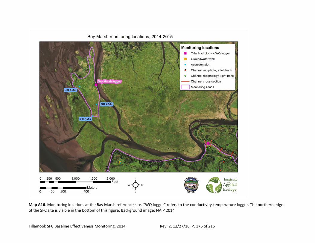
Tillamook SFC Baseline Effectiveness Monitoring, 2014 Rev. 2, 12/27/16, P. 176 of 215
Map A16. Monitoring locations at the Bay Marsh reference site. “WQ logger” refers to the conductivity-temperature logger. The northern edge
of the SFC site is visible in the bottom of this figure. Background image: NAIP 2014
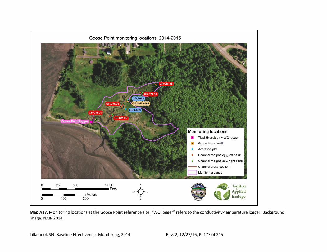
Tillamook SFC Baseline Effectiveness Monitoring, 2014 Rev. 2, 12/27/16, P. 177 of 215
Map A17. Monitoring locations at the Goose Point reference site. “WQ logger” refers to the conductivity-temperature logger. Background
image: NAIP 2014
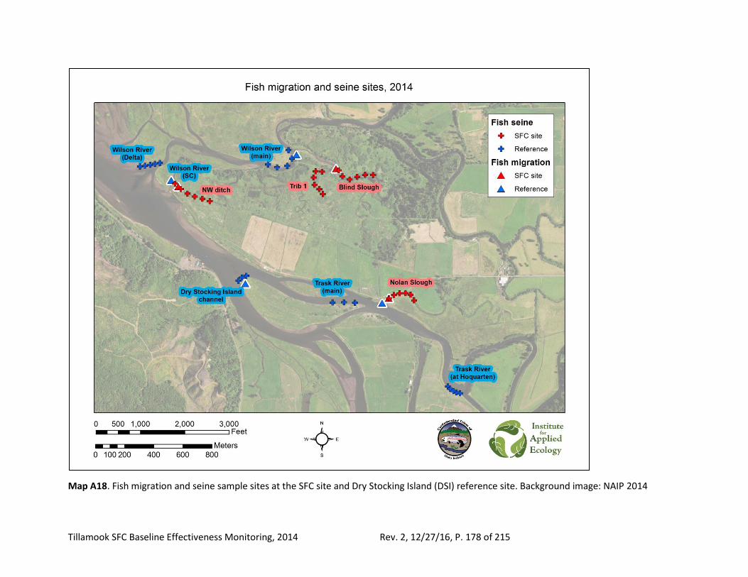
Tillamook SFC Baseline Effectiveness Monitoring, 2014 Rev. 2, 12/27/16, P. 178 of 215
Map A18. Fish migration and seine sample sites at the SFC site and Dry Stocking Island (DSI) reference site. Background image: NAIP 2014
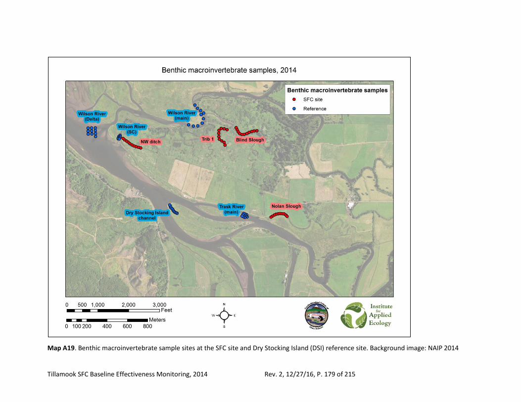
Tillamook SFC Baseline Effectiveness Monitoring, 2014 Rev. 2, 12/27/16, P. 179 of 215
Map A19. Benthic macroinvertebrate sample sites at the SFC site and Dry Stocking Island (DSI) reference site. Background image: NAIP 2014
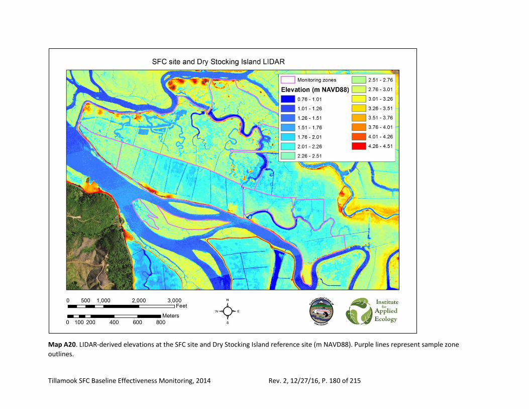
Tillamook SFC Baseline Effectiveness Monitoring, 2014 Rev. 2, 12/27/16, P. 180 of 215
Map A20. LIDAR-derived elevations at the SFC site and Dry Stocking Island reference site (m NAVD88). Purple lines represent sample zone
outlines.
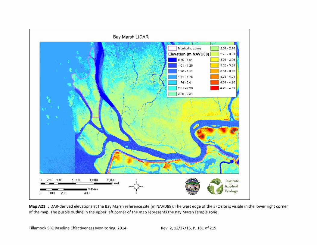
Tillamook SFC Baseline Effectiveness Monitoring, 2014 Rev. 2, 12/27/16, P. 181 of 215
Map A21. LIDAR-derived elevations at the Bay Marsh reference site (m NAVD88). The west edge of the SFC site is visible in the lower right corner
of the map. The purple outline in the upper left corner of the map represents the Bay Marsh sample zone.
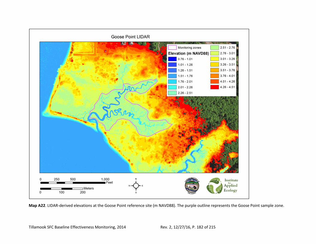
Tillamook SFC Baseline Effectiveness Monitoring, 2014 Rev. 2, 12/27/16, P. 182 of 215
Map A22. LIDAR-derived elevations at the Goose Point reference site (m NAVD88). The purple outline represents the Goose Point sample zone.
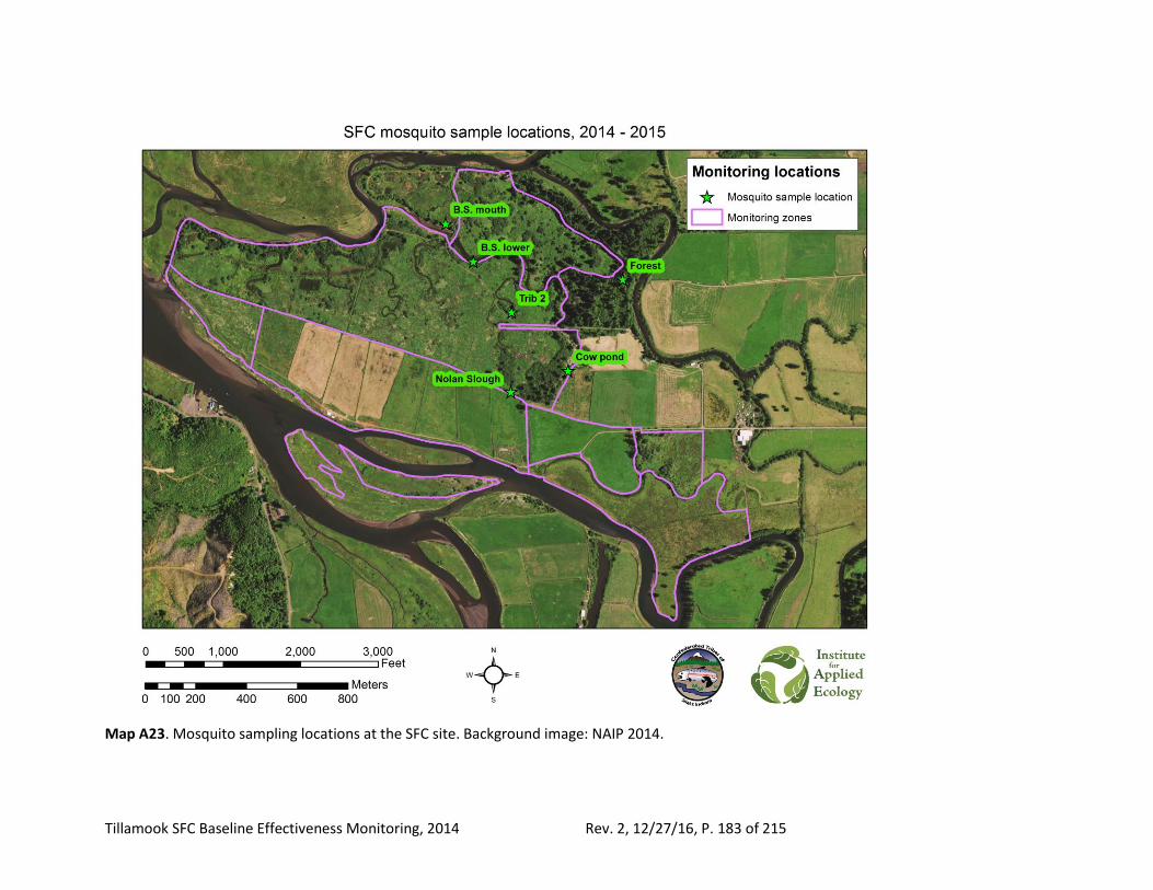
Tillamook SFC Baseline Effectiveness Monitoring, 2014 Rev. 2, 12/27/16, P. 183 of 215
Map A23. Mosquito sampling locations at the SFC site. Background image: NAIP 2014.
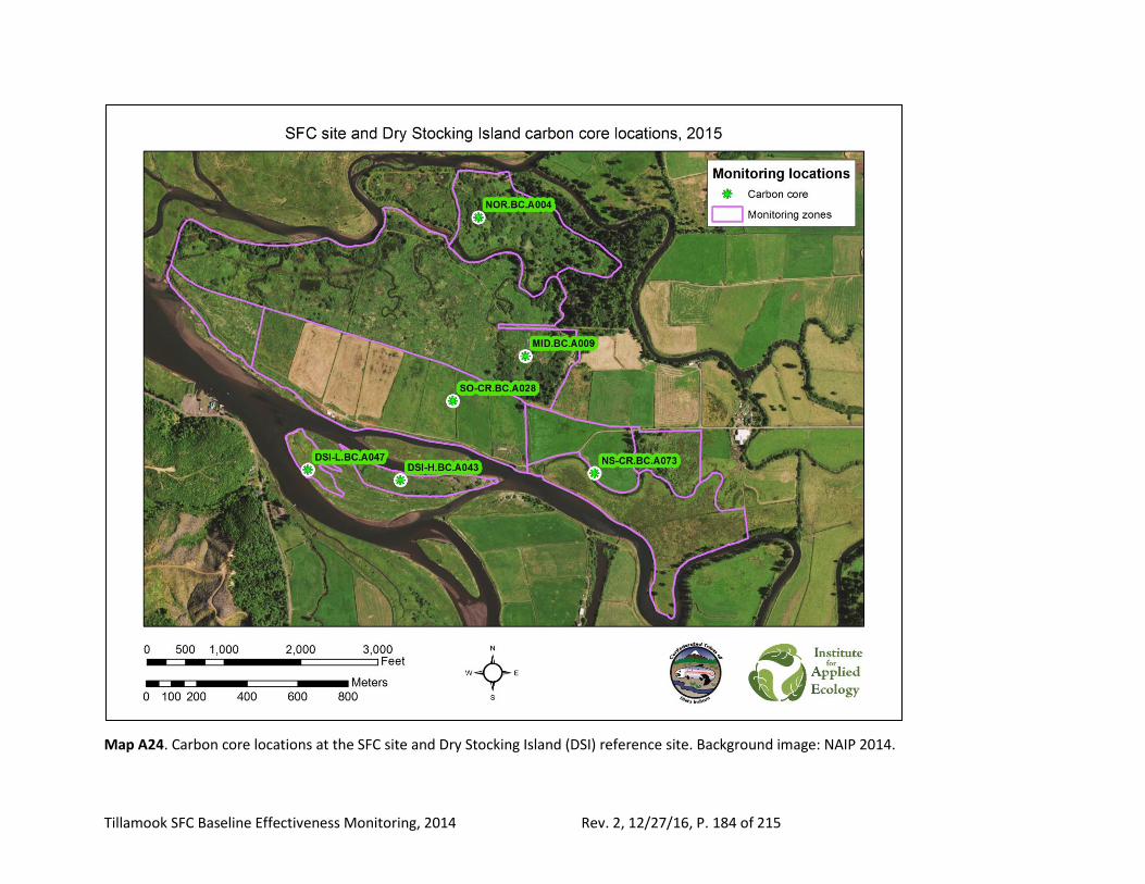
Tillamook SFC Baseline Effectiveness Monitoring, 2014 Rev. 2, 12/27/16, P. 184 of 215
Map A24. Carbon core locations at the SFC site and Dry Stocking Island (DSI) reference site. Background image: NAIP 2014.
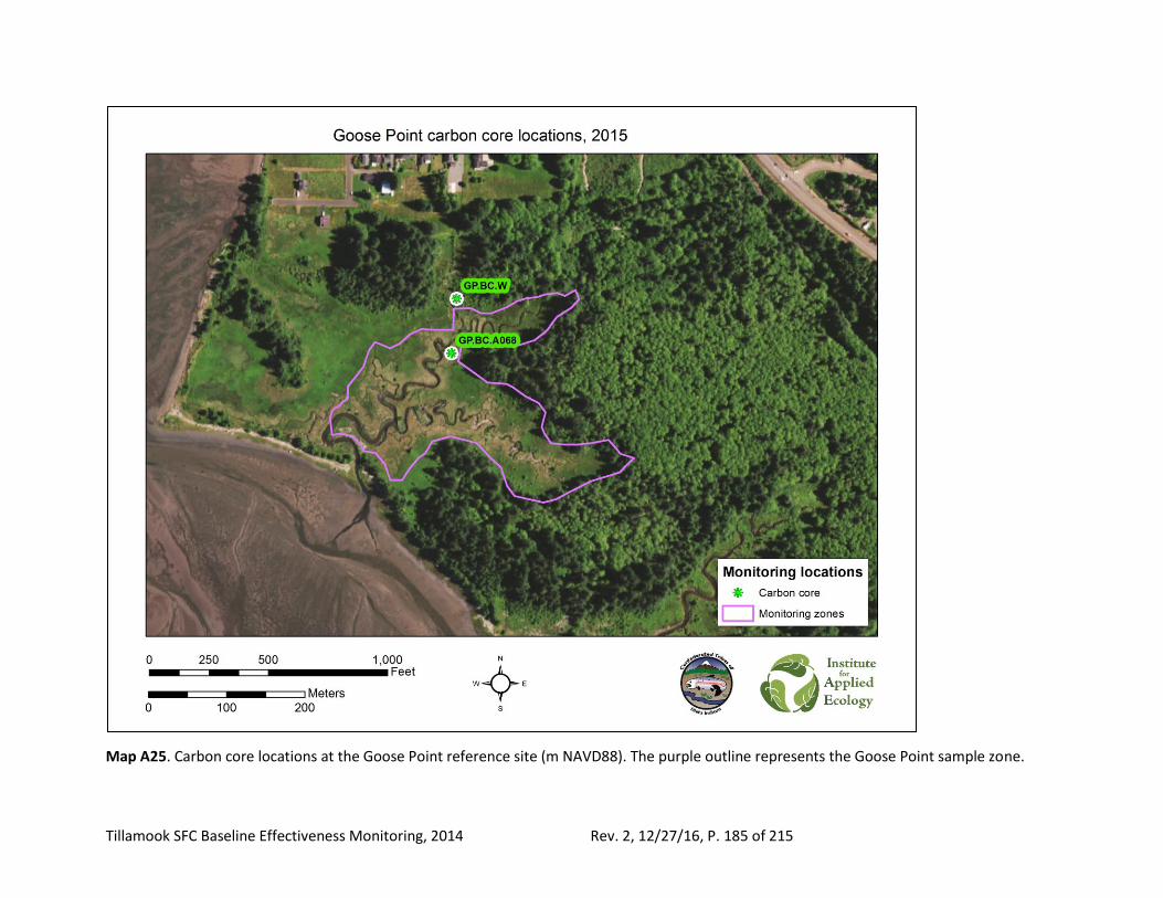
Tillamook SFC Baseline Effectiveness Monitoring, 2014 Rev. 2, 12/27/16, P. 185 of 215
Map A25. Carbon core locations at the Goose Point reference site (m NAVD88). The purple outline represents the Goose Point sample zone.
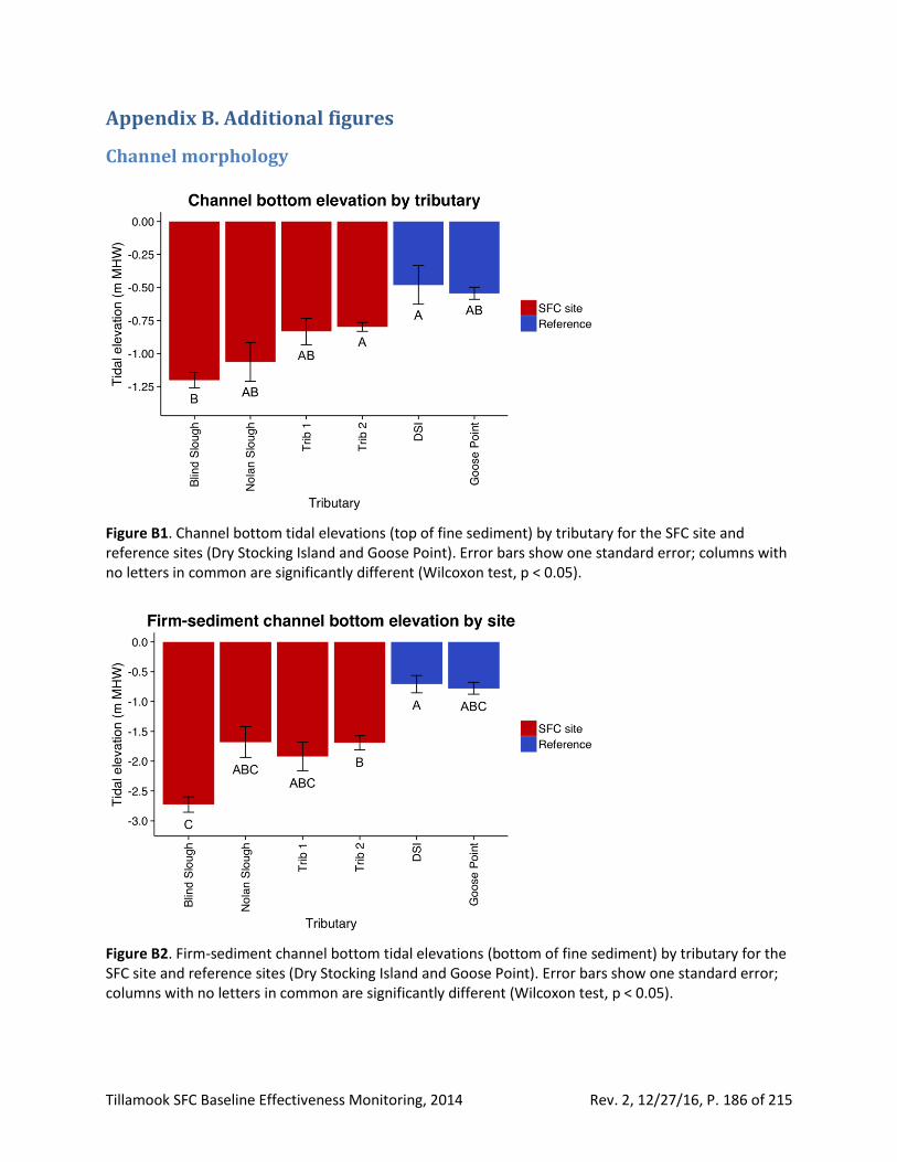
Tillamook SFC Baseline Effectiveness Monitoring, 2014 Rev. 2, 12/27/16, P. 186 of 215
Appendix B. Additional figures
Channel morphology
Figure B1. Channel bottom tidal elevations (top of fine sediment) by tributary for the SFC site and reference sites (Dry Stocking Island and Goose Point). Error bars show one standard error; columns with no letters in common are significantly different (Wilcoxon test, p < 0.05).
Figure B2. Firm-sediment channel bottom tidal elevations (bottom of fine sediment) by tributary for the SFC site and reference sites (Dry Stocking Island and Goose Point). Error bars show one standard error; columns with no letters in common are significantly different (Wilcoxon test, p < 0.05).
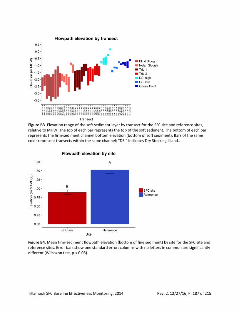
Tillamook SFC Baseline Effectiveness Monitoring, 2014 Rev. 2, 12/27/16, P. 187 of 215
Figure B3. Elevation range of the soft sediment layer by transect for the SFC site and reference sites, relative to MHW. The top of each bar represents the top of the soft sediment. The bottom of each bar represents the firm-sediment channel bottom elevation (bottom of soft sediment). Bars of the same color represent transects within the same channel; “DSI” indicates Dry Stocking Island..
Figure B4. Mean firm-sediment flowpath elevation (bottom of fine sediment) by site for the SFC site and reference sites. Error bars show one standard error; columns with no letters in common are significantly different (Wilcoxon test, p < 0.05).
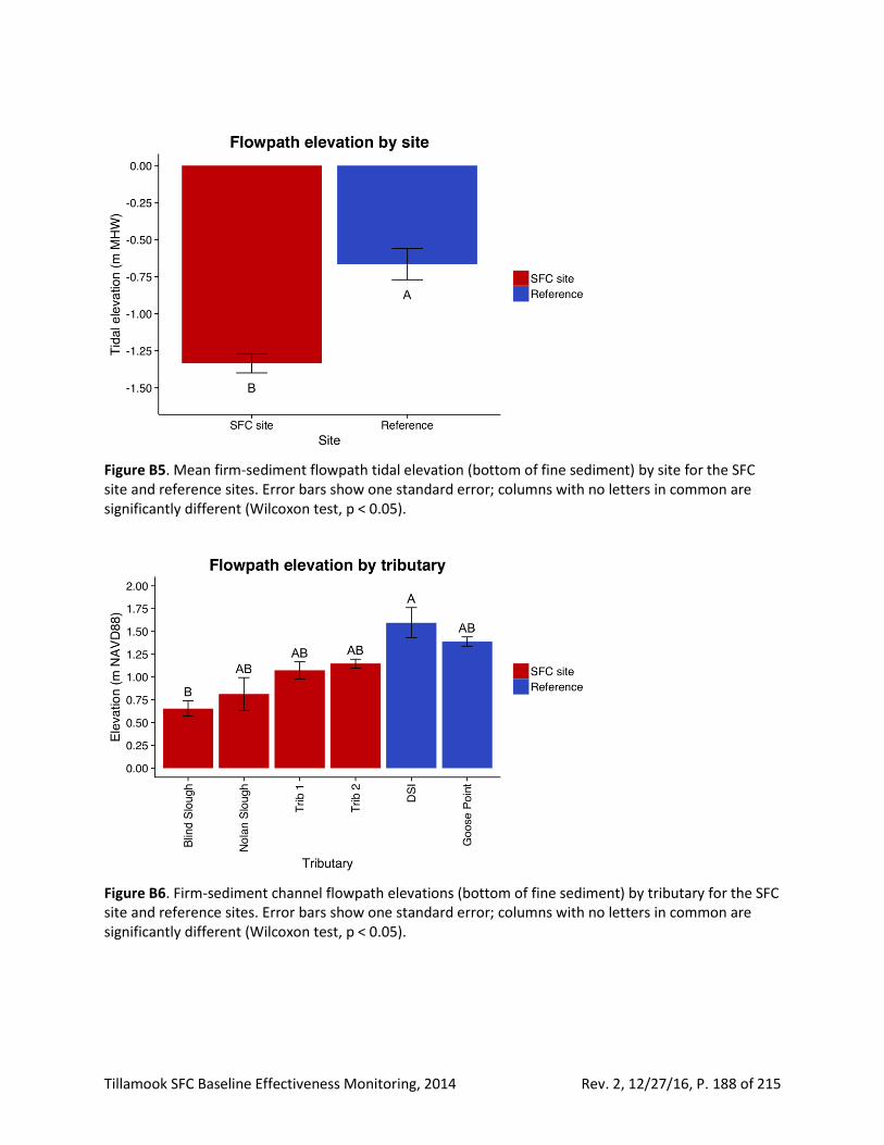
Tillamook SFC Baseline Effectiveness Monitoring, 2014 Rev. 2, 12/27/16, P. 188 of 215
Figure B5. Mean firm-sediment flowpath tidal elevation (bottom of fine sediment) by site for the SFC site and reference sites. Error bars show one standard error; columns with no letters in common are significantly different (Wilcoxon test, p < 0.05).
Figure B6. Firm-sediment channel flowpath elevations (bottom of fine sediment) by tributary for the SFC site and reference sites. Error bars show one standard error; columns with no letters in common are significantly different (Wilcoxon test, p < 0.05).
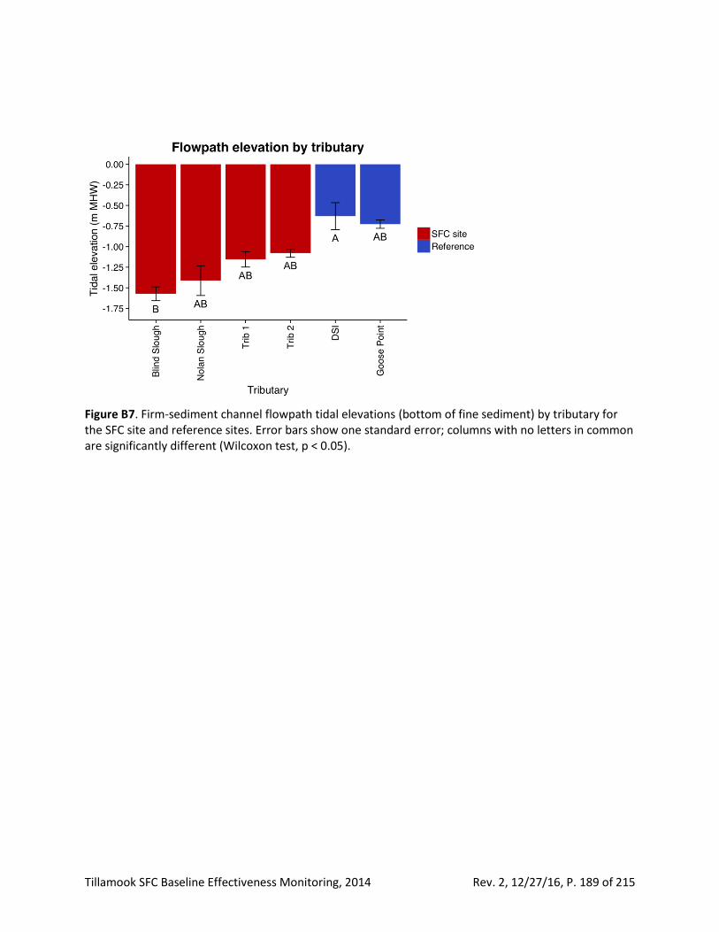
Tillamook SFC Baseline Effectiveness Monitoring, 2014 Rev. 2, 12/27/16, P. 189 of 215
Figure B7. Firm-sediment channel flowpath tidal elevations (bottom of fine sediment) by tributary for the SFC site and reference sites. Error bars show one standard error; columns with no letters in common are significantly different (Wilcoxon test, p < 0.05).
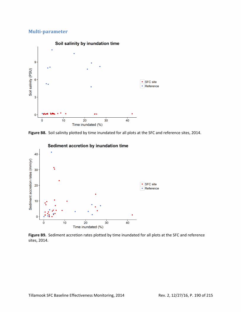
Tillamook SFC Baseline Effectiveness Monitoring, 2014 Rev. 2, 12/27/16, P. 190 of 215
Multi-parameter
Figure B8. Soil salinity plotted by time inundated for all plots at the SFC and reference sites, 2014.
Figure B9. Sediment accretion rates plotted by time inundated for all plots at the SFC and reference sites, 2014.
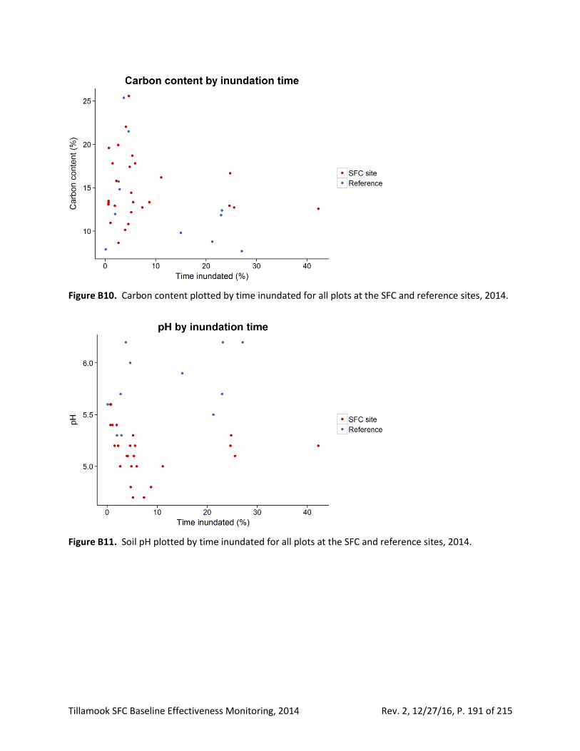
Tillamook SFC Baseline Effectiveness Monitoring, 2014 Rev. 2, 12/27/16, P. 191 of 215
Figure B10. Carbon content plotted by time inundated for all plots at the SFC and reference sites, 2014.
Figure B11. Soil pH plotted by time inundated for all plots at the SFC and reference sites, 2014.
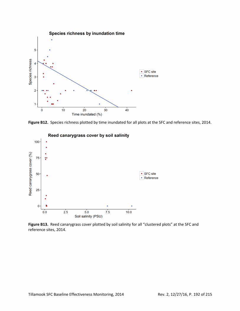
Tillamook SFC Baseline Effectiveness Monitoring, 2014 Rev. 2, 12/27/16, P. 192 of 215
Figure B12. Species richness plotted by time inundated for all plots at the SFC and reference sites, 2014.
Figure B13. Reed canarygrass cover plotted by soil salinity for all “clustered plots” at the SFC and reference sites, 2014.
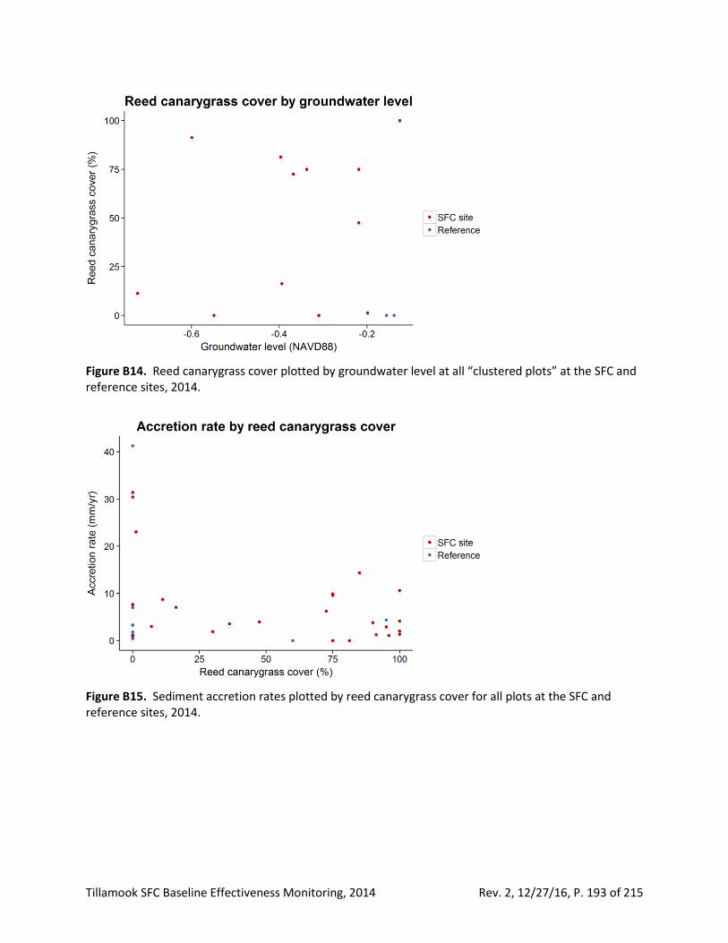
Tillamook SFC Baseline Effectiveness Monitoring, 2014 Rev. 2, 12/27/16, P. 193 of 215
Figure B14. Reed canarygrass cover plotted by groundwater level at all “clustered plots” at the SFC and reference sites, 2014.
Figure B15. Sediment accretion rates plotted by reed canarygrass cover for all plots at the SFC and reference sites, 2014.
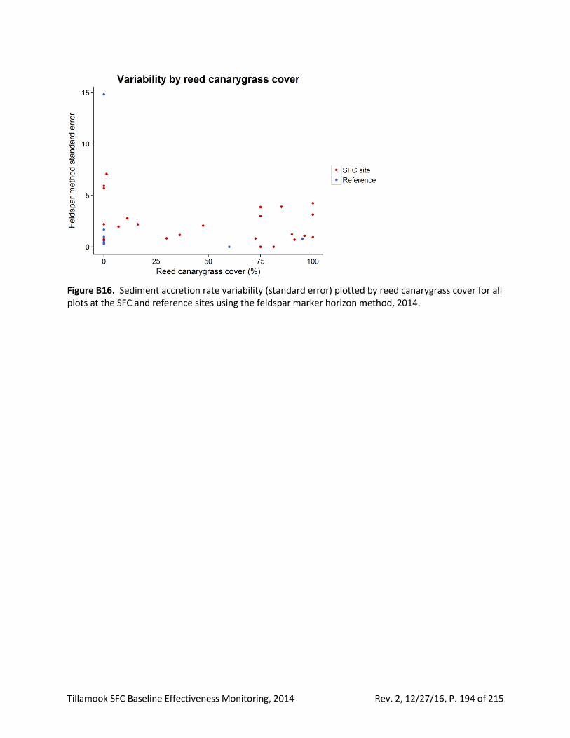
Tillamook SFC Baseline Effectiveness Monitoring, 2014 Rev. 2, 12/27/16, P. 194 of 215
Figure B16. Sediment accretion rate variability (standard error) plotted by reed canarygrass cover for all plots at the SFC and reference sites using the feldspar marker horizon method, 2014.
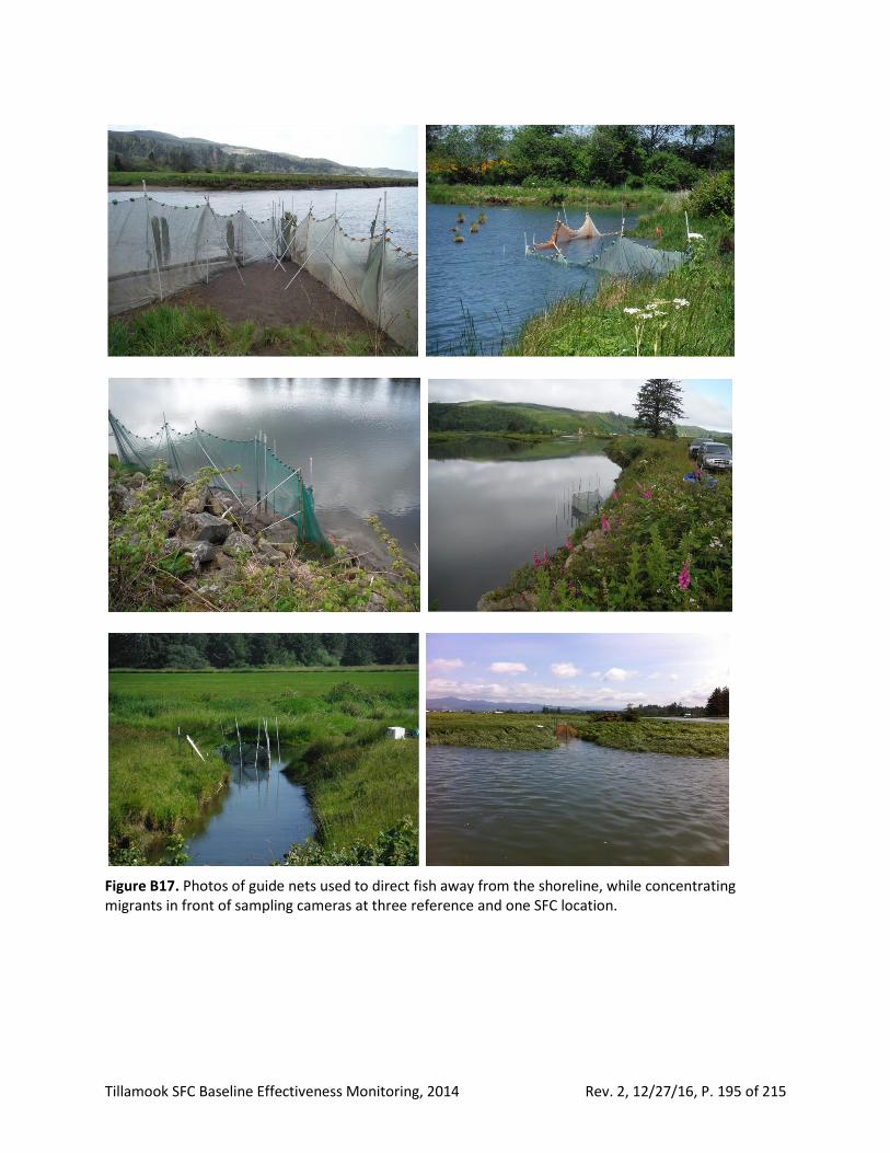
Tillamook SFC Baseline Effectiveness Monitoring, 2014 Rev. 2, 12/27/16, P. 195 of 215
Figure B17. Photos of guide nets used to direct fish away from the shoreline, while concentrating migrants in front of sampling cameras at three reference and one SFC location.
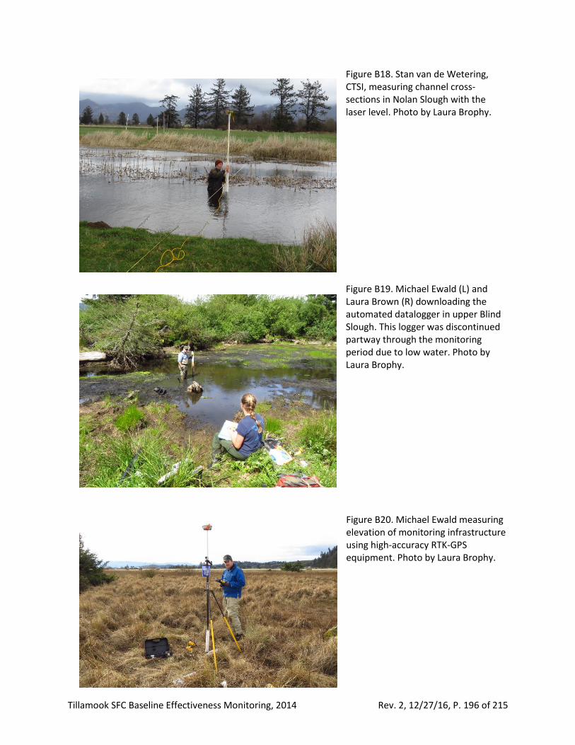
Tillamook SFC Baseline Effectiveness Monitoring, 2014 Rev. 2, 12/27/16, P. 196 of 215
Figure B18. Stan van de Wetering, CTSI, measuring channel cross-sections in Nolan Slough with the laser level. Photo by Laura Brophy. Figure B19. Michael Ewald (L) and Laura Brown (R) downloading the automated datalogger in upper Blind Slough. This logger was discontinued partway through the monitoring period due to low water. Photo by Laura Brophy.
Figure B20. Michael Ewald measuring elevation of monitoring infrastructure using high-accuracy RTK-GPS equipment. Photo by Laura Brophy.
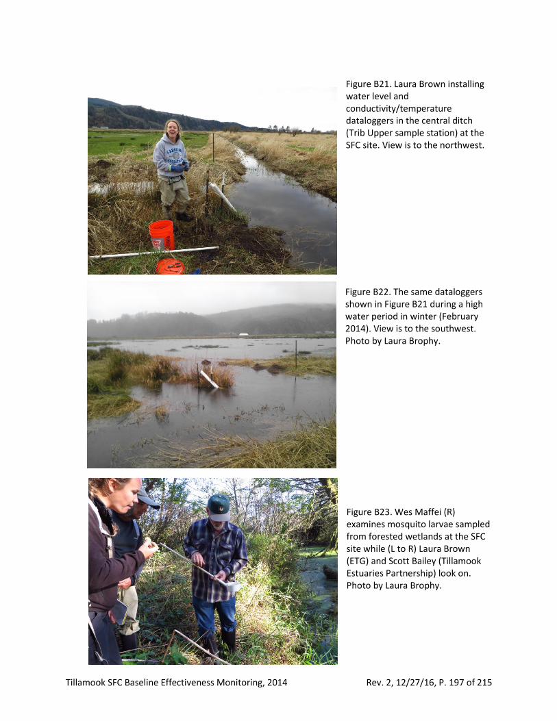
Tillamook SFC Baseline Effectiveness Monitoring, 2014 Rev. 2, 12/27/16, P. 197 of 215
Figure B21. Laura Brown installing water level and conductivity/temperature dataloggers in the central ditch (Trib Upper sample station) at the SFC site. View is to the northwest. Figure B22. The same dataloggers shown in Figure B21 during a high water period in winter (February 2014). View is to the southwest. Photo by Laura Brophy. Figure B23. Wes Maffei (R) examines mosquito larvae sampled from forested wetlands at the SFC site while (L to R) Laura Brown (ETG) and Scott Bailey (Tillamook Estuaries Partnership) look on. Photo by Laura Brophy.
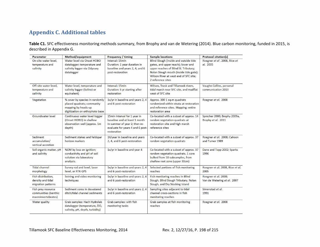
Tillamook SFC Baseline Effectiveness Monitoring, 2014 Rev. 2, 12/27/16, P. 198 of 215
Appendix C. Additional tables Table C1. SFC effectiveness monitoring methods summary, from Brophy and van de Wetering (2014). Blue carbon monitoring, funded in 2015, is described in Appendix G.
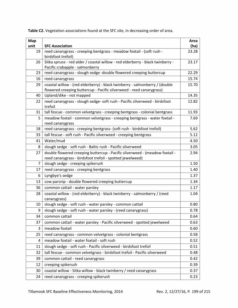
Tillamook SFC Baseline Effectiveness Monitoring, 2014 Rev. 2, 12/27/16, P. 199 of 215
Table C2. Vegetation associations found at the SFC site, in decreasing order of area.
Map unit SFC Association
Area (ha)
19 reed canarygrass - creeping bentgrass - meadow foxtail - (soft rush - birdsfoot trefoil)
23.28
26 Sitka spruce - red alder / coastal willow - red elderberry - black twinberry - Pacific crabapple - salmonberry
23.17
23 reed canarygrass - slough sedge -double flowered creeping buttercup 22.29
16 reed canarygrass 15.74
29 coastal willow - (red elderberry) - black twinberry - salmonberry / (double flowered creeping buttercup - Pacific silverweed - reed canarygrass)
15.70
40 Upland/dike - not mapped 14.35
22 reed canarygrass - slough sedge- soft rush - Pacific silverweed - birdsfoot trefoil
12.82
31 tall fescue - common velvetgrass - creeping bentgrass - colonial bentgrass 11.93
5 meadow foxtail - common velvetgrass - creeping bentgrass - water foxtail - reed canarygrass
7.69
18 reed canarygrass - creeping bentgrass- (soft rush - birdsfoot trefoil) 5.62
33 tall fescue - soft rush - Pacific silverweed - creeping bentgrass 5.12
41 Water/mud 4.50
8 slough sedge - soft rush - Baltic rush - Pacific silverweed 3.05
27 double flowered creeping buttercup - Pacific silverweed - (meadow foxtail - reed canarygrass - birdsfoot trefoil - spotted jewelweed)
2.94
7 slough sedge - creeping spikerush 1.50
17 reed canarygrass - creeping bentgrass 1.40
6 Lyngbye's sedge 1.37
13 cow parsnip - double flowered creeping buttercup 1.34
36 common cattail - water parsley 1.17
28 coastal willow - (red elderberry) - black twinberry - salmonberry / (reed canarygrass)
1.04
10 slough sedge - soft rush - water parsley - common cattail 0.80
9 slough sedge - soft rush - water parsley - (reed canarygrass) 0.78
34 common cattail 0.64
37 common cattail - water parsley - Pacific silverweed - spotted jewelweed 0.63
3 meadow foxtail 0.60
25 reed canarygrass - common velvetgrass - colonial bentgrass 0.58
4 meadow foxtail - water foxtail - soft rush 0.52
11 slough sedge - soft rush - Pacific silverweed - birdsfoot trefoil 0.51
32 tall fescue - common velvetgrass - birdsfoot trefoil - Pacific silverweed 0.48
39 common cattail - reed canarygrass 0.42
12 creeping spikerush 0.39
30 coastal willow - Sitka willow - black twinberry / reed canarygrass 0.37
24 reed canarygrass - creeping spikerush 0.23
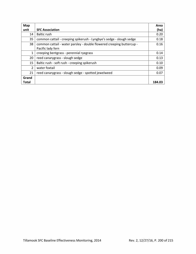
Tillamook SFC Baseline Effectiveness Monitoring, 2014 Rev. 2, 12/27/16, P. 200 of 215
Map unit SFC Association
Area (ha)
14 Baltic rush 0.20
35 common cattail - creeping spikerush - Lyngbye's sedge - slough sedge 0.18
38 common cattail - water parsley - double flowered creeping buttercup - Pacific lady fern
0.16
1 creeping bentgrass - perennial ryegrass 0.14
20 reed canarygrass - slough sedge 0.13
15 Baltic rush - soft rush - creeping spikerush 0.10
2 water foxtail 0.09
21 reed canarygrass - slough sedge - spotted jewelweed 0.07
Grand Total
184.03
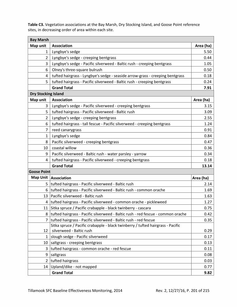
Tillamook SFC Baseline Effectiveness Monitoring, 2014 Rev. 2, 12/27/16, P. 201 of 215
Table C3. Vegetation associations at the Bay Marsh, Dry Stocking Island, and Goose Point reference sites, in decreasing order of area within each site.
Bay Marsh
Map unit Association Area (ha)
1 Lyngbye's sedge 5.50
2 Lyngbye's sedge - creeping bentgrass 0.44
3 Lyngbye's sedge - Pacific silverweed - Baltic rush - creeping bentgrass 1.05
6 Olney's three-square bulrush 0.50
4 tufted hairgrass - Lyngbye's sedge - seaside arrow-grass - creeping bentgrass 0.18
5 tufted hairgrass - Pacific silverweed - Baltic rush - creeping bentgrass 0.24
Grand Total 7.91
Dry Stocking Island
Map unit Association Area (ha)
3 Lyngbye's sedge - Pacific silverweed - creeping bentgrass 3.15
5 tufted hairgrass - Pacific silverweed - Baltic rush 3.09
2 Lyngbye's sedge - creeping bentgrass 2.55
6 tufted hairgrass - tall fescue - Pacific silverweed - creeping bentgrass 1.24
7 reed canarygrass 0.91
1 Lyngbye's sedge 0.84
8 Pacific silverweed - creeping bentgrass 0.47
10 coastal willow 0.36
9 Pacific silverweed - Baltic rush - water parsley - yarrow 0.34
4 tufted hairgrass - Pacific silverweed - creeping bentgrass 0.18
Grand Total 13.14
Goose Point
Map Unit Association Area (ha)
5 tufted hairgrass - Pacific silverweed - Baltic rush 2.14
6 tufted hairgrass - Pacific silverweed - Baltic rush - common orache 1.69
13 Pacific silverweed - Baltic rush 1.63
4 tufted hairgrass - Pacific silverweed - common orache - pickleweed 1.27
11 Sitka spruce / Pacific crabapple - black twinberry - cascara 0.75
8 tufted hairgrass - Pacific silverweed - Baltic rush - red fescue - common orache 0.42
7 tufted hairgrass - Pacific silverweed - Baltic rush - red fescue 0.35
12 Sitka spruce / Pacific crabapple - black twinberry / tufted hairgrass - Pacific silverweed - Baltic rush 0.29
1 slough sedge - Pacific silverweed 0.17
10 saltgrass - creeping bentgrass 0.13
3 tufted hairgrass - common orache - red fescue 0.11
9 saltgrass 0.08
2 tufted hairgrass 0.03
14 Upland/dike - not mapped 0.77
Grand Total 9.82
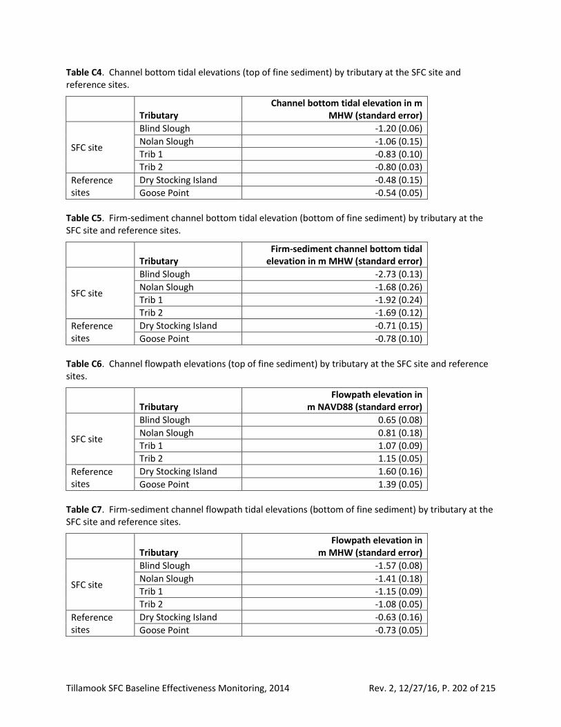
Tillamook SFC Baseline Effectiveness Monitoring, 2014 Rev. 2, 12/27/16, P. 202 of 215
Table C4. Channel bottom tidal elevations (top of fine sediment) by tributary at the SFC site and reference sites.
Tributary
Channel bottom tidal elevation in m MHW (standard error)
SFC site
Blind Slough -1.20 (0.06)
Nolan Slough -1.06 (0.15)
Trib 1 -0.83 (0.10)
Trib 2 -0.80 (0.03)
Reference sites
Dry Stocking Island -0.48 (0.15)
Goose Point -0.54 (0.05)
Table C5. Firm-sediment channel bottom tidal elevation (bottom of fine sediment) by tributary at the SFC site and reference sites.
Tributary
Firm-sediment channel bottom tidal elevation in m MHW (standard error)
SFC site
Blind Slough -2.73 (0.13)
Nolan Slough -1.68 (0.26)
Trib 1 -1.92 (0.24)
Trib 2 -1.69 (0.12)
Reference sites
Dry Stocking Island -0.71 (0.15)
Goose Point -0.78 (0.10)
Table C6. Channel flowpath elevations (top of fine sediment) by tributary at the SFC site and reference sites.
Tributary
Flowpath elevation in m NAVD88 (standard error)
SFC site
Blind Slough 0.65 (0.08)
Nolan Slough 0.81 (0.18)
Trib 1 1.07 (0.09)
Trib 2 1.15 (0.05)
Reference sites
Dry Stocking Island 1.60 (0.16)
Goose Point 1.39 (0.05)
Table C7. Firm-sediment channel flowpath tidal elevations (bottom of fine sediment) by tributary at the SFC site and reference sites.
Tributary
Flowpath elevation in m MHW (standard error)
SFC site
Blind Slough -1.57 (0.08)
Nolan Slough -1.41 (0.18)
Trib 1 -1.15 (0.09)
Trib 2 -1.08 (0.05)
Reference sites
Dry Stocking Island -0.63 (0.16)
Goose Point -0.73 (0.05)
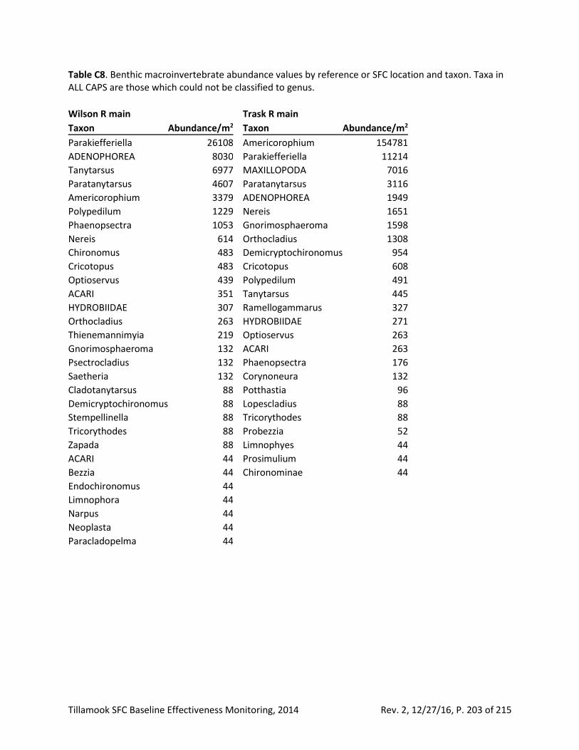
Tillamook SFC Baseline Effectiveness Monitoring, 2014 Rev. 2, 12/27/16, P. 203 of 215
Table C8. Benthic macroinvertebrate abundance values by reference or SFC location and taxon. Taxa in ALL CAPS are those which could not be classified to genus.
Wilson R main Trask R main
Taxon Abundance/m2 Taxon Abundance/m2
Parakiefferiella 26108 Americorophium 154781
ADENOPHOREA 8030 Parakiefferiella 11214
Tanytarsus 6977 MAXILLOPODA 7016
Paratanytarsus 4607 Paratanytarsus 3116
Americorophium 3379 ADENOPHOREA 1949
Polypedilum 1229 Nereis 1651
Phaenopsectra 1053 Gnorimosphaeroma 1598
Nereis 614 Orthocladius 1308
Chironomus 483 Demicryptochironomus 954
Cricotopus 483 Cricotopus 608
Optioservus 439 Polypedilum 491
ACARI 351 Tanytarsus 445
HYDROBIIDAE 307 Ramellogammarus 327
Orthocladius 263 HYDROBIIDAE 271
Thienemannimyia 219 Optioservus 263
Gnorimosphaeroma 132 ACARI 263
Psectrocladius 132 Phaenopsectra 176
Saetheria 132 Corynoneura 132
Cladotanytarsus 88 Potthastia 96
Demicryptochironomus 88 Lopescladius 88
Stempellinella 88 Tricorythodes 88
Tricorythodes 88 Probezzia 52
Zapada 88 Limnophyes 44
ACARI 44 Prosimulium 44
Bezzia 44 Chironominae 44
Endochironomus 44
Limnophora 44
Narpus 44
Neoplasta 44
Paracladopelma 44
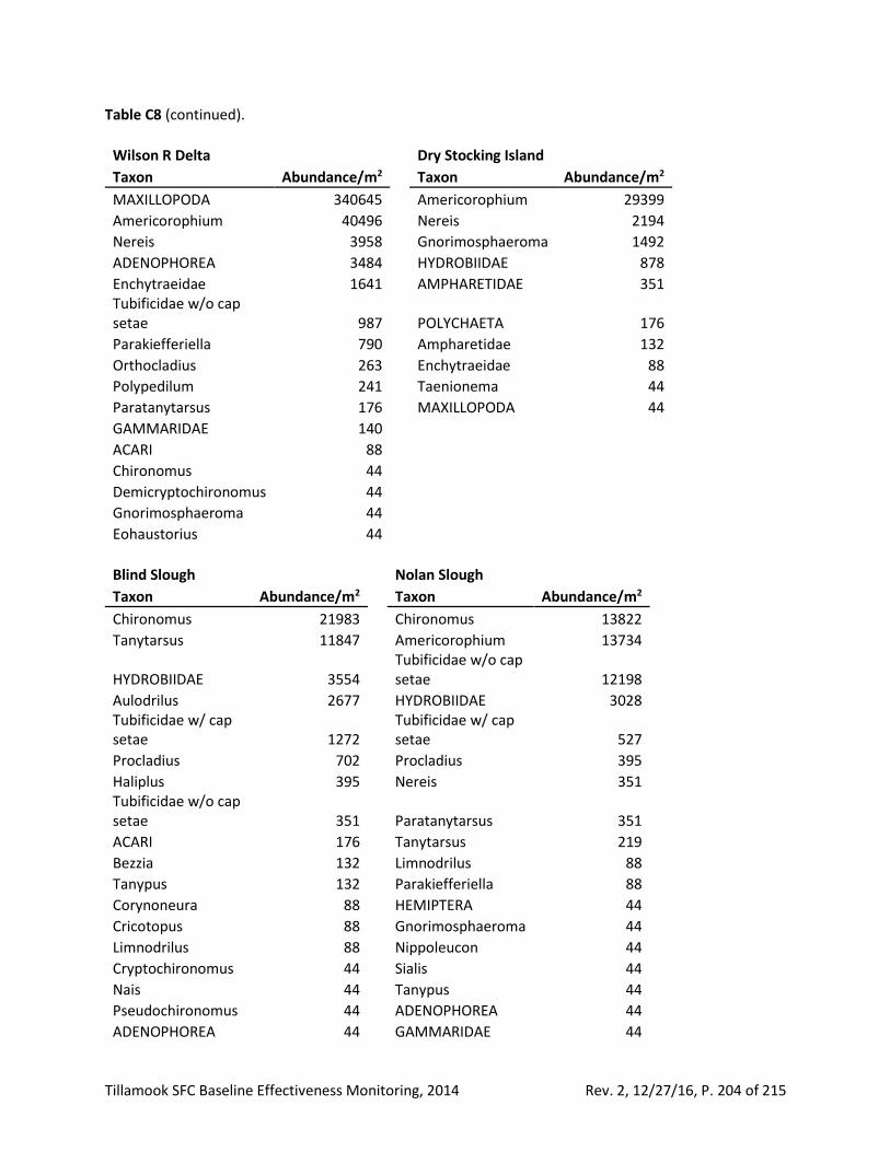
Tillamook SFC Baseline Effectiveness Monitoring, 2014 Rev. 2, 12/27/16, P. 204 of 215
Table C8 (continued).
Wilson R Delta Dry Stocking Island
Taxon Abundance/m2 Taxon Abundance/m2
MAXILLOPODA 340645 Americorophium 29399
Americorophium 40496 Nereis 2194
Nereis 3958 Gnorimosphaeroma 1492
ADENOPHOREA 3484 HYDROBIIDAE 878
Enchytraeidae 1641 AMPHARETIDAE 351 Tubificidae w/o cap setae 987 POLYCHAETA 176
Parakiefferiella 790 Ampharetidae 132
Orthocladius 263 Enchytraeidae 88
Polypedilum 241 Taenionema 44
Paratanytarsus 176 MAXILLOPODA 44
GAMMARIDAE 140
ACARI 88
Chironomus 44
Demicryptochironomus 44
Gnorimosphaeroma 44
Eohaustorius 44
Blind Slough
Nolan Slough
Taxon Abundance/m2 Taxon Abundance/m2
Chironomus 21983 Chironomus 13822
Tanytarsus 11847 Americorophium 13734
HYDROBIIDAE 3554 Tubificidae w/o cap setae 12198
Aulodrilus 2677 HYDROBIIDAE 3028 Tubificidae w/ cap setae 1272
Tubificidae w/ cap setae 527
Procladius 702 Procladius 395
Haliplus 395 Nereis 351 Tubificidae w/o cap setae 351 Paratanytarsus 351
ACARI 176 Tanytarsus 219
Bezzia 132 Limnodrilus 88
Tanypus 132 Parakiefferiella 88
Corynoneura 88 HEMIPTERA 44
Cricotopus 88 Gnorimosphaeroma 44
Limnodrilus 88 Nippoleucon 44
Cryptochironomus 44 Sialis 44
Nais 44 Tanypus 44
Pseudochironomus 44 ADENOPHOREA 44
ADENOPHOREA 44 GAMMARIDAE 44
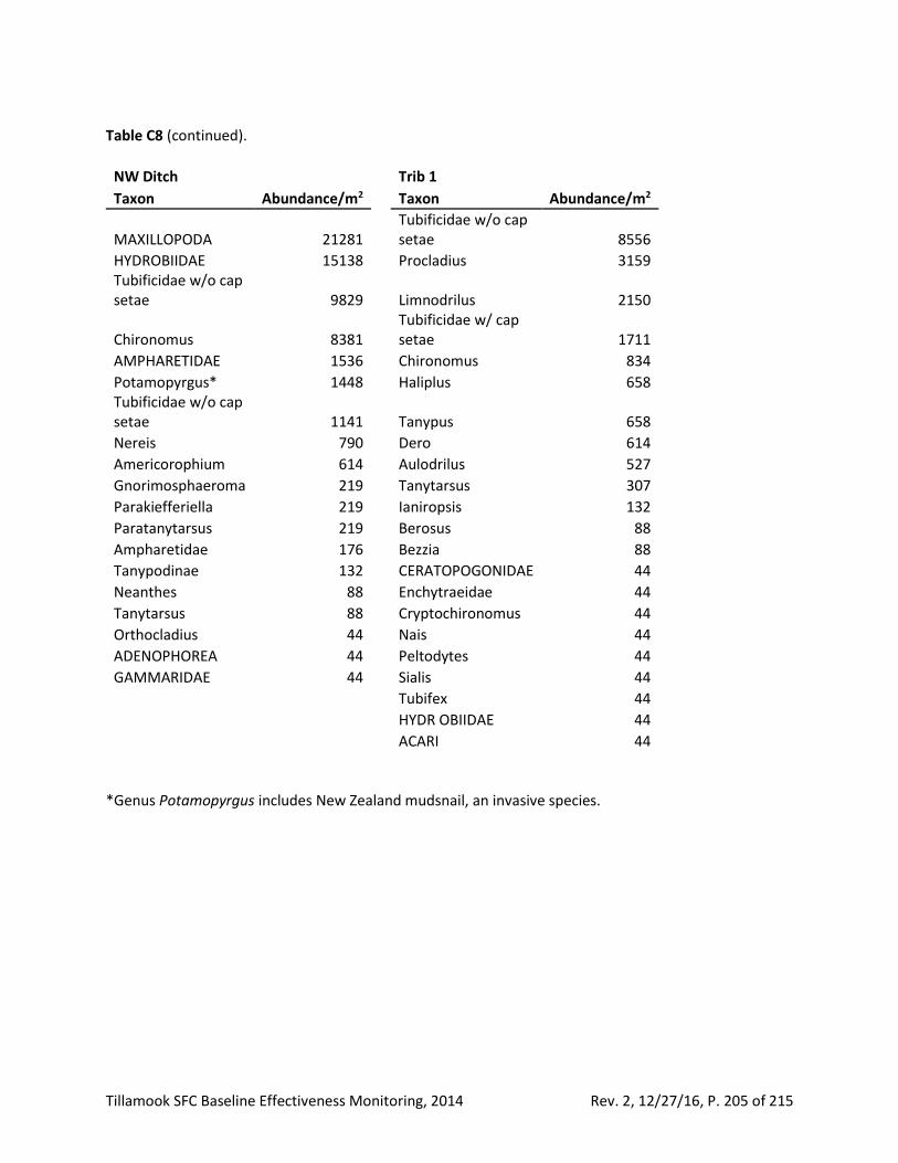
Tillamook SFC Baseline Effectiveness Monitoring, 2014 Rev. 2, 12/27/16, P. 205 of 215
Table C8 (continued).
NW Ditch Trib 1
Taxon Abundance/m2 Taxon Abundance/m2
MAXILLOPODA 21281 Tubificidae w/o cap setae 8556
HYDROBIIDAE 15138 Procladius 3159 Tubificidae w/o cap setae 9829 Limnodrilus 2150
Chironomus 8381 Tubificidae w/ cap setae 1711
AMPHARETIDAE 1536 Chironomus 834
Potamopyrgus* 1448 Haliplus 658 Tubificidae w/o cap setae 1141 Tanypus 658
Nereis 790 Dero 614
Americorophium 614 Aulodrilus 527
Gnorimosphaeroma 219 Tanytarsus 307
Parakiefferiella 219 Ianiropsis 132
Paratanytarsus 219 Berosus 88
Ampharetidae 176 Bezzia 88
Tanypodinae 132 CERATOPOGONIDAE 44
Neanthes 88 Enchytraeidae 44
Tanytarsus 88 Cryptochironomus 44
Orthocladius 44 Nais 44
ADENOPHOREA 44 Peltodytes 44
GAMMARIDAE 44 Sialis 44
Tubifex 44
HYDR OBIIDAE 44
ACARI 44 *Genus Potamopyrgus includes New Zealand mudsnail, an invasive species.
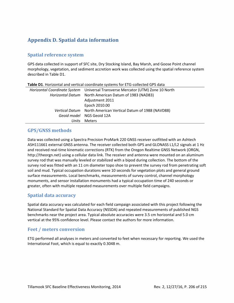
Tillamook SFC Baseline Effectiveness Monitoring, 2014 Rev. 2, 12/27/16, P. 206 of 215
Appendix D. Spatial data information
Spatial reference system
GPS data collected in support of SFC site, Dry Stocking Island, Bay Marsh, and Goose Point channel morphology, vegetation, and sediment accretion work was collected using the spatial reference system described in Table D1. Table D1. Horizontal and vertical coordinate systems for ETG-collected GPS data
Horizontal Coordinate System Universal Transverse Mercator (UTM) Zone 10 North Horizontal Datum North American Datum of 1983 (NAD83)
Adjustment 2011 Epoch 2010.00
Vertical Datum North American Vertical Datum of 1988 (NAVD88) Geoid model NGS Geoid 12A
Units Meters
GPS/GNSS methods
Data was collected using a Spectra Precision ProMark 220 GNSS receiver outfitted with an Ashtech ASH111661 external GNSS antenna. The receiver collected both GPS and GLONASS L1/L2 signals at 1 Hz and received real-time kinematic corrections (RTK) from the Oregon Realtime GNSS Network (ORGN, http://theorgn.net) using a cellular data link. The receiver and antenna were mounted on an aluminum survey rod that was manually leveled or stabilized with a bipod during collection. The bottom of the survey rod was fitted with an 11 cm diameter topo shoe to prevent the survey rod from penetrating soft soil and mud. Typical occupation durations were 10 seconds for vegetation plots and general ground surface measurements. Local benchmarks, measurements of survey control, channel morphology monuments, and sensor installation monuments had a typical occupation time of 240 seconds or greater, often with multiple repeated measurements over multiple field campaigns.
Spatial data accuracy
Spatial data accuracy was calculated for each field campaign associated with this project following the National Standard for Spatial Data Accuracy (NSSDA) and repeated measurements of published NGS benchmarks near the project area. Typical absolute accuracies were 3.5 cm horizontal and 5.0 cm vertical at the 95% confidence level. Please contact the authors for more information.
Feet / meters conversion
ETG performed all analyses in meters and converted to feet when necessary for reporting. We used the International Foot, which is equal to exactly 0.3048 m.
Tillamook SFC Baseline Effectiveness Monitoring, 2014 Rev. 2, 12/27/16, P. 207 of 215
Appendix E. Plant community metrics across habitats Species richness was significantly higher in the high marsh, compared to the lower marsh, but not significantly different between the SFC site and reference sites (Tables E1 and E2, Figure E1). There was no difference between high and low marsh, or between the SFC and reference sites in total plant cover; however, the SFC site had significantly lower native plant cover, and significantly higher non-native cover when compared to nearby reference sites. There was no significant difference between low marsh and high marsh in native or non-native plant cover (Table E1, Figure E1). Table E1. Summary of two-way ANOVA results for vegetation metrics in two habitat types (low and high marsh) at the SFC and reference sites. Bold text indicates significant differences (p < 0.05).
Treatment p-value
Species richness
sites 0.74
habitat < 0.0001
sites x habitat 0.28
Total plant cover
sites 0.53
habitat 0.55
sites x habitat 0.56
Native plant cover
sites < 0.0001
habitat 0.47
sites x habitat 0.88
Non-native plant cover
sites < 0.0001
habitat 0.52
sites x habitat 0.78
Table E2. Average and standard error of plant community metrics within habitats at the SFC site and reference sites, 2014.
Habitat
Average species
richness (standard
error)
Average total cover
(standard error)
Average native cover
(standard error)
Average non-native
cover (standard
error)
SFC site low marsh 2.3 (0.3) 19.9 (0.2) 19.9 (5.9) 76.7 (5.9)
high marsh 4.3 (0.2) 99.2 (0.8) 24.2 (5.2) 75.0 (5.2)
Reference sites low marsh 1.7 (0.8) 99.5 (0.4) 79.9 (11.4) 19.5 (11.2)
high marsh 4.5 (0.1) 100.0 (0.0) 86.6 (2.4) 13.4 (2.5)
Tillamook SFC Baseline Effectiveness Monitoring, 2014 Rev. 2, 12/27/16, P. 208 of 215
Figure E1. Average plant species richness, total cover, native cover and non-native cover for the SFC site and reference sites in the low marsh and high marsh. Error bars show one standard error; columns with no letters in common are significantly different (ANOVA test, p < 0.05).
Tillamook SFC Baseline Effectiveness Monitoring, 2014 Rev. 2, 12/27/16, P. 209 of 215
Appendix F. Sediment accretion and erosion rates using sediment stake method As mentioned in the methods section, sediment stakes were used as a backup to feldspar plots, or to indicate any significant erosion at a plot. They were not expected to provide high-accuracy data on sediment accretion or erosion. Nonetheless, patterns in accretion rates determined using the feldspar marker horizon method were similar to those determined using the sediment stake method (Figure F1-Figure F5), though the rates differed between the two methods (Table F1, Table 38 above). Average sediment accretion rates at the SFC site and nearby reference sites were 12.7 and 14.5 mm/year respectively. There were no consistent relationships between rates of accretion between the two methods (Figure F6 and F7), and standard error was much higher using the sediment stake method, when compared to the feldspar marker horizon method (Figure F6 and F7). Because of the high variability in accretion as measured using the sediment stake method, we recommend that the data from the feldspar marker horizon method should be used preferentially to understand contrasts in accretion rates between the SFC site and the reference sites. Table F1. Average and standard error of sediment accretion within zones at the SFC site and reference sites for the sediment stake method. Negative numbers are erosion; positive numbers are accretion. Standard errors could not be calculated for South zone – no crop or Goose Point (n = 1).
Zone Average sediment accretion
rate, mm/yr (standard error)
SFC site
North zone 16.2 (2.6)
Middle zone 7.6 (5.3)
South zone no crop 35.4 (NA)
South zone crop 15.3 (6.2)
Nolan ungrazed 2.7 (4.4)
Reference sites
Bay Marsh 17.9 (4.3)
Dry Stocking Island – low marsh 11.7 (3.1)
Dry Stocking Island – high marsh 12.9 (1.4)
Goose Point 23.2 (NA)
Tillamook SFC Baseline Effectiveness Monitoring, 2014 Rev. 2, 12/27/16, P. 210 of 215
Figure F1. Average sediment accretion rates for the SFC site and reference sites using the sediment stake method. Error bars show one standard error; columns with no letters in common are significantly different (t-test, p < 0.05).
Figure F2. Average sediment accretion rates among zones using the sediment stake method. Error bars show one standard error; columns with no letters in common are significantly different (ANOVA test, p < 0.05).
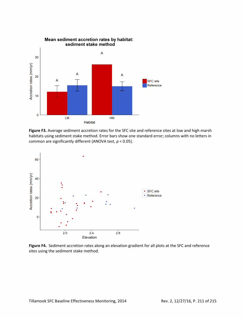
Tillamook SFC Baseline Effectiveness Monitoring, 2014 Rev. 2, 12/27/16, P. 211 of 215
Figure F3. Average sediment accretion rates for the SFC site and reference sites at low and high marsh habitats using sediment stake method. Error bars show one standard error; columns with no letters in common are significantly different (ANOVA test, p < 0.05).
Figure F4. Sediment accretion rates along an elevation gradient for all plots at the SFC and reference sites using the sediment stake method.
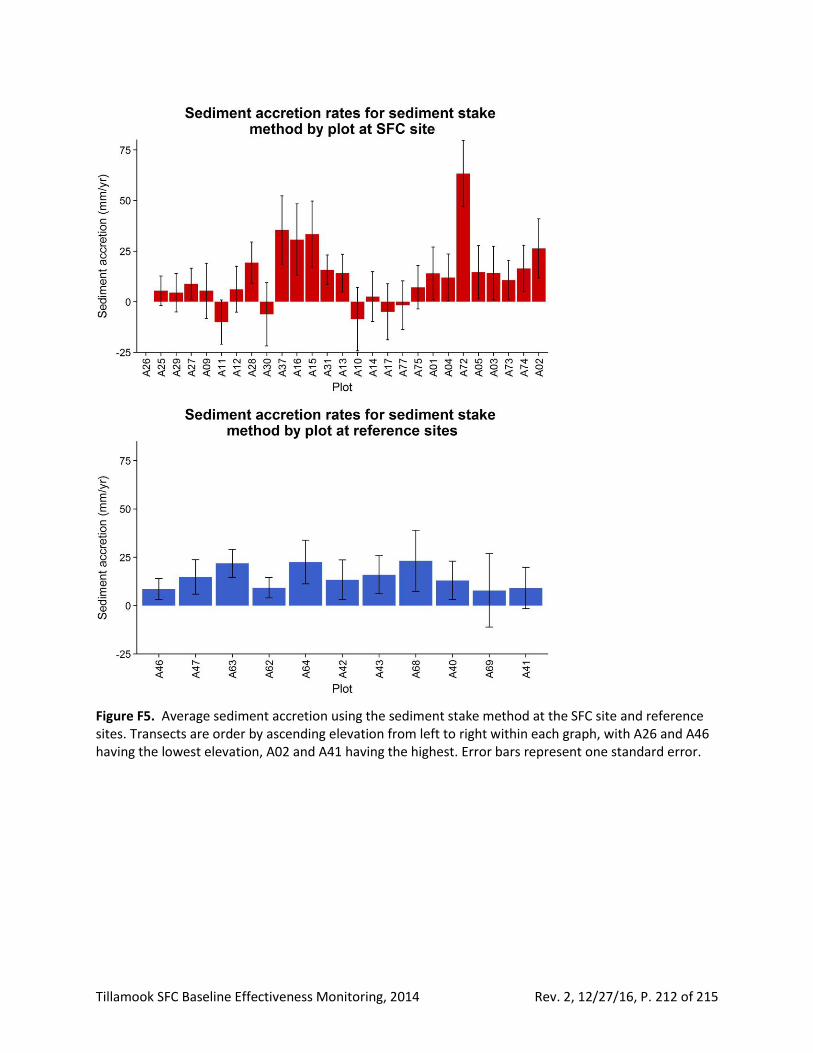
Tillamook SFC Baseline Effectiveness Monitoring, 2014 Rev. 2, 12/27/16, P. 212 of 215
Figure F5. Average sediment accretion using the sediment stake method at the SFC site and reference sites. Transects are order by ascending elevation from left to right within each graph, with A26 and A46 having the lowest elevation, A02 and A41 having the highest. Error bars represent one standard error.
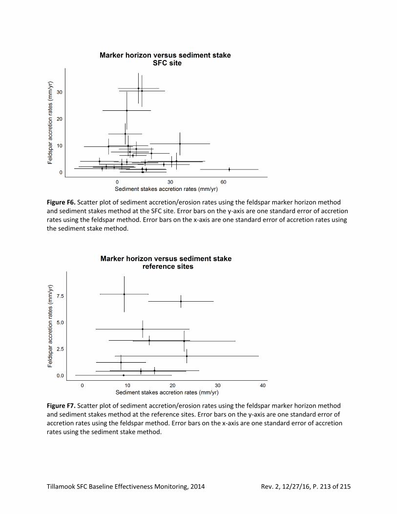
Tillamook SFC Baseline Effectiveness Monitoring, 2014 Rev. 2, 12/27/16, P. 213 of 215
Figure F6. Scatter plot of sediment accretion/erosion rates using the feldspar marker horizon method and sediment stakes method at the SFC site. Error bars on the y-axis are one standard error of accretion rates using the feldspar method. Error bars on the x-axis are one standard error of accretion rates using the sediment stake method.
Figure F7. Scatter plot of sediment accretion/erosion rates using the feldspar marker horizon method and sediment stakes method at the reference sites. Error bars on the y-axis are one standard error of accretion rates using the feldspar method. Error bars on the x-axis are one standard error of accretion rates using the sediment stake method.
Tillamook SFC Baseline Effectiveness Monitoring, 2014 Rev. 2, 12/27/16, P. 214 of 215
Appendix G. “Blue” carbon accumulation: Progress report
“Blue” carbon accumulation overview
Coastal ecosystems, such as seagrass meadows, mangrove forests, and intertidal salt marshes, store and sequester carbon. Tidal wetlands, in particular, store 3-5 times more carbon than tropical forests, and due to high sediment delivery, high organic content in soils, and sheltered settings, Pacific Northwest tidal wetlands have high potential for carbon sequestration (Murray et al. 2011, Crooks et al. 2014). Quantifying current carbon storage and rates of carbon sequestration at the SFC site and reference sites allows us to quantify carbon accumulation rates, estimate carbon losses that occur when the site was diked and drained, and predict post-restoration carbon accumulations rates at the SFC site.
Project activities performed to date ETG collected four carbon soil cores at the SFC site and six cores at the SFC reference sites (two each at Bay Marsh, Dry Stocking Island, and Goose Point) in April 2015 (Table G1, Maps A24-A25). At the SFC site, a core was taken from the North, Middle, Nolan crop, and South crop zones; all cores were 1.5 m long and co-located with accretion plots. At Bay Marsh and Dry Stocking Island, both a 3 m core and a 1.5 m core were taken and co-located with accretion plots. At Goose Point, two long (3 m) cores were taken, one that was co-located with an accretion plot, and the other was taken in the willows and no co-located. Table G1. Locations of carbon cores at the SFC site and reference sites. Easting and Northing represent UTM Zone 10 N coordinates in meters. Sensor elevations are expressed in meters NAVD88 (Geoid 12A). Locations are shown in Maps A24 and A25. See Appendix D for Spatial Reference System information.
Wetland zone Site Easting Northing
Elevation in meters
NAVD88
SFC site
North zone A04 431479 5036430 2.22
Middle zone A09 431672 5035883 1.86
South zone crop A28 431378 5035704 2.01
Nolan crop A73 431941 5035419 2.37
Reference sites
Bay Marsh A63 430016 5036970 2.12
Bay Marsh A64 430164 5036813 2.31
Dry Stocking Island low A47 430806 5035439 2.00
Dry Stocking Island high A43 431171 5035388 2.60
Goose Point A68 430963 5039939 2.66
Goose Point Willow 430959 5040017 NA
All cores have been taken to Oregon State University (OSU) for processing and analysis. At OSU, cores will be sampled for isotopic activity, specifically for 210Pb and 137Cs, allowing the calculation of carbon accumulation rates. The majority of these cores were co-located with sediment accretion plots to give us side-by-side comparisons of accretion rates by methods, and so we could include information from our vegetation monitoring in our final analyses.
Upcoming project activities The field work component of data collection is complete. Upcoming activities involve analyzing and

Tillamook SFC Baseline Effectiveness Monitoring, 2014 Rev. 2, 12/27/16, P. 215 of 215
interpreting the isotope data in the lab, then relating that information to physical site conditions such as elevation, inundation regime, and salinity; and to biological conditions (particularly vegetation. These data and interpretations will be included in the report to Tillamook County due December 31, 2016. The December 2016 report will also include results from the 2016 sediment accretion sampling.