Spatial and temporal monitoring of soil water content

with an irrigated corn crop cover using surface

electrical resistivity tomography

Didier Michot,1 Yves Benderitter,2 Abel Dorigny,1 Bernard Nicoullaud,1

Dominique King,1 and Alain Tabbagh2

Received 15 July 2002; revised 13 November 2002; accepted 18 February 2003; published 27 May 2003.

[1] A nondestructive and spatially integrated multielectrode method for measuring soilelectrical resistivity was tested in the Beauce region of France during a period of corn cropirrigation to monitor soil water flow over time and in two-dimensional (2-D) withsimultaneous measurements of soil moisture and thermal profiles. The results suggestedthe potential of surface electrical resistivity tomography (ERT) for improving soil scienceand agronomy studies. The method was able to produce a 2-D delimitation of soil horizonsas well as to monitor soil water movement. Soil drainage through water uptake by theroots, the progression of the infiltration front with preferential flow zones, and thedrainage of the plowed horizon were well identified. At the studied stage of corndevelopment (3 months) the soil zones where infiltration and drainage occurred weremainly located under the corn rows. The structural soil characteristics resulting fromagricultural practices or the passage of agricultural equipment were also shown. Two-dimensional sections of soil moisture content were calculated using ERT. The estimateswere made by using independently established ‘‘in situ’’ calibration relationships betweenthe moisture and electrical resistivity of typical soil horizons. The thermal soil profile wasalso considered in the modeling. The results showed a reliable linear relationship betweenthe calculated and measured water contents in the crop horizon. The precision of thecalculation of the specific soil water content, quantified by the root mean square error(RMSE), was 3.63% with a bias corresponding to an overestimation of 1.45%. Theanalysis and monitoring of the spatial variability of the soil moisture content with ERTrepresent two components of a significant tool for better management of soil waterreserves and rational irrigation practices. INDEX TERMS: 0925 Exploration Geophysics: Magnetic

and electrical methods; 1866 Hydrology: Soil moisture; 1875 Hydrology: Unsaturated zone; 5109 Physical

Properties of Rocks: Magnetic and electrical properties; KEYWORDS: soil moisture, unsaturated soil, electrical

resistivity tomography, monitoring, infiltration, drying

Citation: Michot, D., Y. Benderitter, A. Dorigny, B. Nicoullaud, D. King, and A. Tabbagh, Spatial and temporal monitoring of soil

water content with an irrigated corn crop cover using surface electrical resistivity tomography, Water Resour. Res., 39(5), 1138,

doi:10.1029/2002WR001581, 2003.

1. Introduction

[2] To provide an adequate water supply for growingcorn, one must obtain precise knowledge of the soil mois-ture state. It is necessary to monitor water content changesin the field to measure water losses through infiltration andevapotranspiration. Better knowledge of soil water flow alsogives a better understanding of the behavior and transport ofagricultural pollutants. In consequence, a rational samplingstrategy can be established to study the active time of themolecules residence.[3] As soil electrical resistivity is related to its water

content, the general aim of this study is to determine soil

moisture with electrical resistivity, or more specifically torelate soil electrical resistivity changes with water contentchanges in an unsaturated soil.[4] The first step of this study is to verify the capacity of

the multielectrode method to monitor over time the soilwater dynamics under an irrigated corn crop (Zea mays L.),particularly water infiltration and soil drainage by rootuptake. The second step is to obtain 2-D soil water contentsections after calibration of the electrical resistivity of typicalsoil horizons according to their moisture. The third step is totest the calculated water content with regard to soil watercontent measured simultaneously with electrical resistivity.

2. Review of Soil Water Content Measurements

2.1. Standard Measurements

[5] In addition to direct weighing method, soil water andmoisture profiles can be obtained with numerous indirectmethods where sensors are placed in the soil at different

1Institut National de la Recherche Agronomique Orleans, Unite deScience du Sol, Olivet, France.

2UMR 7619 ‘‘Sisyphe’’, UMPC, CNRS, case 105, Paris, France.

Copyright 2003 by the American Geophysical Union.0043-1397/03/2002WR001581

SBH 14 - 1

WATER RESOURCES RESEARCH, VOL. 39, NO. 5, 1138, doi:10.1029/2002WR001581, 2003

depths. The neutron probe [Gardner and Kirkam, 1952;Bavel et al., 1956] is a reliable water content measurementmethod [Chanasyk and Naeth, 1996], but its use is limitedbecause radioactive source produces numerous constraints.Measurements of dielectric soil properties by TDR (timedomain reflectometry) probes [Topp et al., 1980] orcapacitance sensors [Bell et al., 1987; Dean et al., 1987]avoid the use of radioactive sources. Time domainreflectometry is a technique to estimate the volumetric soilwater content. It is based on the determination of theapparent dielectric constant K of soil. This quantity iscalculated from the velocity of propagation of an electro-magnetic signal in the frequency range of 1 MHz to 1 GHzalong a transmission line in the soil, neglecting losses alongthe line as reviewed by Topp and Davis [1985]. Soilvolumetric water content q is calculated using an empiricalrelationship, which is independent of soil type, soil density,soil temperature and soluble salt content [Topp et al., 1980]:

q¼�5:3� 10�2 þ 2:92�10�2K � 5:5�10�4K2 þ 4:3� 10�6K3

ð1Þ

The precision of volumetric water content measurement isabout ±2%. The water potential, which must be known tounderstand water flow in an unsaturated soil, is measuredwith a tensiometer. Water infiltration into the soil is notuniform. The vertical and horizontal soil water content ishighly variable and depends on preferential flow directions[Kung., 1990a, 1990b; Herkelrath et al., 1991; Ritsema etal., 1993; Ritsema and Dekker, 1994; Flury et al., 1994].Soil moisture sensors yield only restricted information andare often not representative of the spatial soil waterdistribution. Now, improved measurement techniques andautomated methods, such as multiTDR systems have madepossible soil moisture changes monitoring over time atdifferent locations and detection of preferential water flowdirections [Heimovaara and Boulten, 1990; Herkelrath etal., 1991]. Still, these systems offer information at only aseries of point locations rather than continuously at the fieldscale. Moreover, inserting moisture sensors disturbs the soilstructure and the water flow [Rothe et al., 1997].[6] Many alternative methods have been tested in order to

monitor water flow within the soil over time. Soluble dyetracers added to soil water have been used [Kung, 1990a,1990b; Flury et al., 1994; Scanlon and Goldsmith, 1997].With this method, the spatial distribution of the dye tracer inthe soil can be observed and therefore the infiltration zonecan be determined. As a soil pit must be dug at theexperimental site to monitor tracer infiltration, the soilstructure is disturbed and the obtained information may notbe representative of the actual processes under investiga-tion. For example, the water flow may be perturbed by thechanged soil drainage induced when a soil pit is dug.[7] Nevertheless, it is difficult to obtain a 2-D or 3-D

representation of the water flow in the soil by exploitingsparse local data. Geophysical surface methods are notintrusive and consequently do not disturb the soil structure.Also, each measurement integrates a greater volume of soil.These methods represent alternative ways of monitoringunsaturated soil water fluxes. The following discussionfocuses on the use of ERT to monitor moisture changes insoil over time.

2.2. Use of Surface Geophysical Methods forEstimating Water Content and Infiltration

[8] Various surface geophysical methods have been usedby hydrogeologists and soil scientists to identify soil waterinfiltration and water flow. In the past, much research hasbeen performed using ground penetrating radar (GPR) todetect buried objects, to delineate geological structures and tomeasure the soil water content [Davis and Annan, 1989;Hubbard et al., 1997; Eppstein and Dougherty, 1998;Weileret al., 1998; Parkin et al., 2000]. The majority of the studieshave produced positive results. Daily and Ramirez [1989]tested dielectric permittivity using borehole electromagnetictomography to map water content changes in a heatedvolcanic ignimbrite. Weiler et al. [1998] concluded that incomparison with TDR measurements, GPR gave promisingresults for nondestructive water content measurements.Hubbard et al. [1997] showed that the joint use of GPR andconventional borehole data improves water saturation es-timates for geological formations. By comparing radar wavevelocity before and after a controlled release of salt water inthe vadose zone, Eppstein and Dougherty [1998] detectedand visualized soil moisture patterns in three dimensions.Recently, Parkin et al. [2000] showed the ad-vantage ofGPR in monitoring soil water content distribution in a ho-rizontal plane located below a wastewater trench. Hubbardet al. [2002] and Huisman et al. [2001] showed how GPRground wave data could be used effectively to map nearsurface changes in water content. GPR performance is opti-mal in a soil with a coarse texture, but the performance dec-reases in electrically conductive media such as clayey soils.[9] The nuclear magnetic resonance (NMR) method uses

the nuclear properties of hydrogen to assess water content. Inthe ground, most hydrogen atoms are found in the watermolecules. The NMR method can detect water directly,whereas conventional geophysical methods provide onlyindirect knowledge of soil moisture. Using NMR, the watercontent distribution and ground porosity versus depth havebeen estimated [Amin et al., 1993; Goldman et al., 1994;Beauce et al., 1996]. However, NMR measurements are notsuitable for superficial soil studies, as the first few metersbelow the land surface constitute a blind zone for thatmethod.[10] Soil electrical resistivity is a function of the textural

and structural characteristics and is particularly sensitive toits water content [Sheets and Hendrickx, 1995]. Soils are aporous medium, made of nonconductive solid particles andcontaining electrolytes solution that can conduct electriccurrent by the movement of the free ions in the bulksolution and ions adsorbed at the matrix surface. Precipita-tion and seasonal variations in soil temperature and soilwater content cause significant changes in the electricalresistivity of the soil [Aaltonen, 1997; Benderitter andSchott, 1999]. Water infiltration and aquifer recharge can bedetected by studies of variations in electrical soundingcurves [Barraud et al., 1979; Cosentino et al., 1979].Groundwater flow direction and velocity can be determinedthrough observation of the electrical resistivity decrease inalluvial deposits following salt water tracer injections[White, 1994]. Recent development of a surface multi-electrode method, known as electrical resistivity tomogra-phy (ERT), offers some interesting perspectives. Thismethod is particularly well suited to the 2-D description

SBH 14 - 2 MICHOT ET AL.: SOIL WATER STUDY USING ELECTRICAL RESISTIVITY

of geological structures perpendicular to the measurementelectrode line [Griffiths and Turnbull, 1985; Griffiths et al.,1990; Shima, 1990; Griffiths and Barker, 1993]. ERTpresents great advantages for monitoring and is used in hy-drological and environmental studies to monitor solutes andfluid flow in porous media. Monitoring of vadose zone wa-ter flow such as water infiltration, root water uptake, bore-hole pumping test effects has been reported by many authors[Barker and Moore, 1998; Benderitter and Schott, 1999;Binley et al., 2001]. Hagrey and Michaelsen [1999], andMichot et al. [2001] adapted the electrode set up to reach afiner resolution in order to monitor soil water infiltration in2-D. Recent progress in modeling and geo-physical 3-Dinversion methods greatly reduced calculation errors andprocessing time [Zhang et al., 1995]. Three-dimensionalmonitoring of small fresh water plume movements throughthe vadose zone has become possible [Park, 1998]. Zhou etal. [2001] also proposed a noninvasive me-thod to monitor,in the field, soil water content changes over time by meansof 3-D electrical tomography. The cited works revealed thecapability of ERT data in monitoring water infiltration inunsaturated soil or through the vadose zone, as is our focus.However, these works did not consider the possibility ofobtaining a water content cross section from ERT data usinga field-scale calibration method and taking into account thesoil thermal profile. This current study, unlike the previousones, investigates water flow dynamics in relation to the soilmanagement (agricultural prac-tices, tillage operations) witha corn crop cover irrigated by sprinkling.

3. Presentation of the Study Site

[11] The study area is located southwest of Paris, in theBeauce region, at Villamblain (Figure 1). The topography isweakly undulating with slopes rarely exceeding 2%. Thealtitude ranges between 121 m and 125 m. The loamy clay

soil has a thickness of 0.3 to 1.2 m over the Beaucelimestone bedrock, containing a large aquifer about between15 and 70 m depth. The water is pumped for crop irrigationand regional drinking water supply.[12] The studied site has a corn crop cover (Zea mays L)

and is irrigated by sprinklers. The experimental plot soil canbe classified as a loamy clay Calcisol developed in a beigecryoturbated limestone deposit according to the French soilreference system [Baize and Girard, 1995]. Because ofnumerous studies about the regional spatial soil distributionand the experimental plot [Isambert and Duval, 1992;Nicoullaud et al., 1997], this Calcisol was chosen as repre-sentative of the soil in the region. A soil pit was dug near theexperimental device to identify the characteristic soil hori-zons (Figure 2). Three reference horizons include the fol-lowing: (1) First is the top horizon, LAci, an organomineral30 cm thick plow layer. It has a loamy clay texture, a finepolyhedral structure and a very high porosity. A plowed panlies beneath its lower boundary. (2) Second is a light brownstructural S horizon with slight weathering, observed at adepth from 30 cm to 75 cm. It is a loamy clay layer withoutcoarse fragments and with a medium polyhedral structureand high porosity. This horizon is subdivided into threeparts: Sci1, Sci2 and Sca3. This division is justified by adecrease in clay content, a gradual weakening of soilstructure and an increase of carbonate inflorescences insideearthworm burrows with depth. (3) Third is the Ck horizon ata 75 cm depth. It is formed of beige cryoturbated and highlyweathered soft limestone rocks. It has a massive structureand a high porosity. This horizon is subdivided into twolayers, Ck(m)1 (75–100 cm) and Ck2 (100–170 cm). On thebasis of simultaneous decrease of clay and silt content andincrease of carbonate content (CaCO3 > 75%) with depth.[13] An auger drilling into the bottom of the soil pit

provides additional information at depth. The Ck2 horizongoes down to a depth of 170 cm. A soft powdery graylimestone mineral horizon Ck3 exists between 170 and 250cm depth. Beyond this, the auger was blocked by a slab ofsublithographic hard gray Beauce Limestone. Table 1 showsparticle size distribution of the fine earth fraction aftercarbonate removal and chemical analysis. The soil isalkaline (pH > 8.2). There is slight recarbonatation of theLAci surface horizon with regard to horizon Sci1, no doubtrelated to the working of the soil and the use of irrigationwater rich in calcium carbonate. The exchange complex issaturated with calcium throughout the soil profile.[14] The corn crop was sown on 21 April 2000 with a

density of 90,000 pl/ha and a distance of 0.80 m betweenrows. The soil was plowed to a depth of 30 cm andreworked on the surface by a harrow to reduce the size ofthe superficial clumps. The corn root profile (on the left ofFigure 2) shows that the corn root density is higher in theplowed horizon between a depth of 0.1 and 0.3 m. The cornroot density decreases rapidly with depth [Nicoullaud et al.,1995]. This is a representative and typical soil of the Beauceregion, which covers 85000 ha. Major soil differences areassociated with only the thickness of the loamy-clay horizonand the CaCO3 content.

4. Field Calibration

[15] A considerable effort has gone toward investigatingthe relationship between the apparent electrical resistivity

Figure 1. Location of the study area.

MICHOT ET AL.: SOIL WATER STUDY USING ELECTRICAL RESISTIVITY SBH 14 - 3

(or its reciprocal, the apparent electrical conductivity), waterconductivity and water content in saturated and unsaturatedporous media. Numerous reviews of these petrophysicalmodels have been published [Bussian, 1983; Worthington,1985; Mualem and Friedman, 1991; Benderitter and Schott,1999] and their respective advantages and drawbacks havebeen discussed. The first model was established for cleansand, i.e. without any clay, in saturated or unsaturatedconditions [Archie, 1942]. This model can not be used forthe soil at our study site, which is a much moreheterogeneous soil that contains clays.Wyllie and Southwick[1954] suggested that an aggregate of conductive particlessaturated with a conductive electrolyte could be modeledwith a three resistor network. Waxman and Smits [1968]proposed the first extensive model of shaly sand formations.They proposed that clay particles contribute exchangecations to the electrolyte thereby increasing the conductivityof the formation. The dual water model suggested byClavier et al. [1977] is based on the assumption that theexchange cations contribute to the conductivity of a claywater which is spatially separated from the bulk waterlocated in the pore space. More complex theoretical

relationship were proposed relying upon properties of asolid phase dispersed in a continuous electrolyte [Bussian,1983] or accounting for the different behavior of ions in thespore space [Revil et al., 1998]. Mualem and Friedman[1991] proposed a model more adapted for soil at any watersaturation but it does not take into account the surfaceconductivity. So, in unsaturated condition this model seemsmore adapted for soil with a coarse texture. The quality of theprediction decreases for fine texture as clayed soil. Mostpublished models are either theoretical and present somephysical limits, or are obtained in laboratory on small soilcores with controlled conditions.[16] We considered the use of both laboratory-derived and

field-derived petrophysical relationships for application toour field-scale ERT data. We attempted to use a laboratorycalibration because it was easier and faster to measure the soilcore electrical resistivity on a vast range of soil moisture.During a drying period, electrical resistivity and water con-tent were measured on a cylindrical soil core from LAci andSci1 loamy-clay horizons. As expected, a high soil electricalresistivity decrease was observed as soil volumetric watercontent increased up to 15%, and when the soil volumetric

Figure 2. Water flow monitoring; experimental setup by 2-D electrical resistivity tomography in itspedological and agricultural context.

Table 1. Physical and Chemical Analyses of a Calcisola

HorizonDepth,cm

C,%

FS,%

CS,%

Fsa,%

Csa,%

CaCO3,% pH

CEC,cmol kg�1

Ca++,cmol kg�1

Na+,cmol kg�1

Mg++,cmol kg�1

K+,cmol kg�1 da

LAci 0–30 32.0 29.2 32.3 2.1 0.4 4.0 8.2 20.3 43.6 0.082 1.12 0.766 1.27Sci1 30–55 32.3 30.4 34.1 1.7 0.2 1.3 8.3 18.0 32.7 0.084 0.83 0.422 1.45Sci2 55–70 29.4 30.1 34.3 1.5 0.1 4.6 8.4 14.4 45.9 0.103 0.64 0.287 -Sca3 70–75 17.1 20.8 24.0 1.1 0.2 36.8 8.6 9.2 44.3 0.078 0.43 0.168 -

Ck(m)1 75–100 13.4 14.4 16.4 1 0.5 54.3 - - - - - - 1.51Ck2 100–120 8.0 4.5 7.5 1.8 0.8 77.4 - - - - - - -

aParticle size analyses following carbonate removal. C, clay; FS, fine silt; CS, coarse silt; FSa: fine sand; CSa: coarse sand (X31-107); da: bulk density.

SBH 14 - 4 MICHOT ET AL.: SOIL WATER STUDY USING ELECTRICAL RESISTIVITY

moisture increased from 15% to 45%, a regular and weakersoil resistivity decrease was remarked. However, these rela-tionships obtained in laboratory were not representativebecause the saturation water conductivity of the soil coreswas different from the natural soil solution electrical con-ductivity in the field. Moreover, we observed a high varia-bility of the soil core electrical resistivity measurement withthe soil sample volume. For the same moisture, an increase inthe soil core volume was always associated with a higherelectrical resistivity value, which suggests that the measure-ment elementary volume of the soil core must be definedbefore using a laboratory relationship. Because of this majorlimitation, we decided instead in this study to develop a field-scale site specific petrophysical model, which we judged tobe more representative of natural conditions.[17] The aims of this field study were (1) to verify that

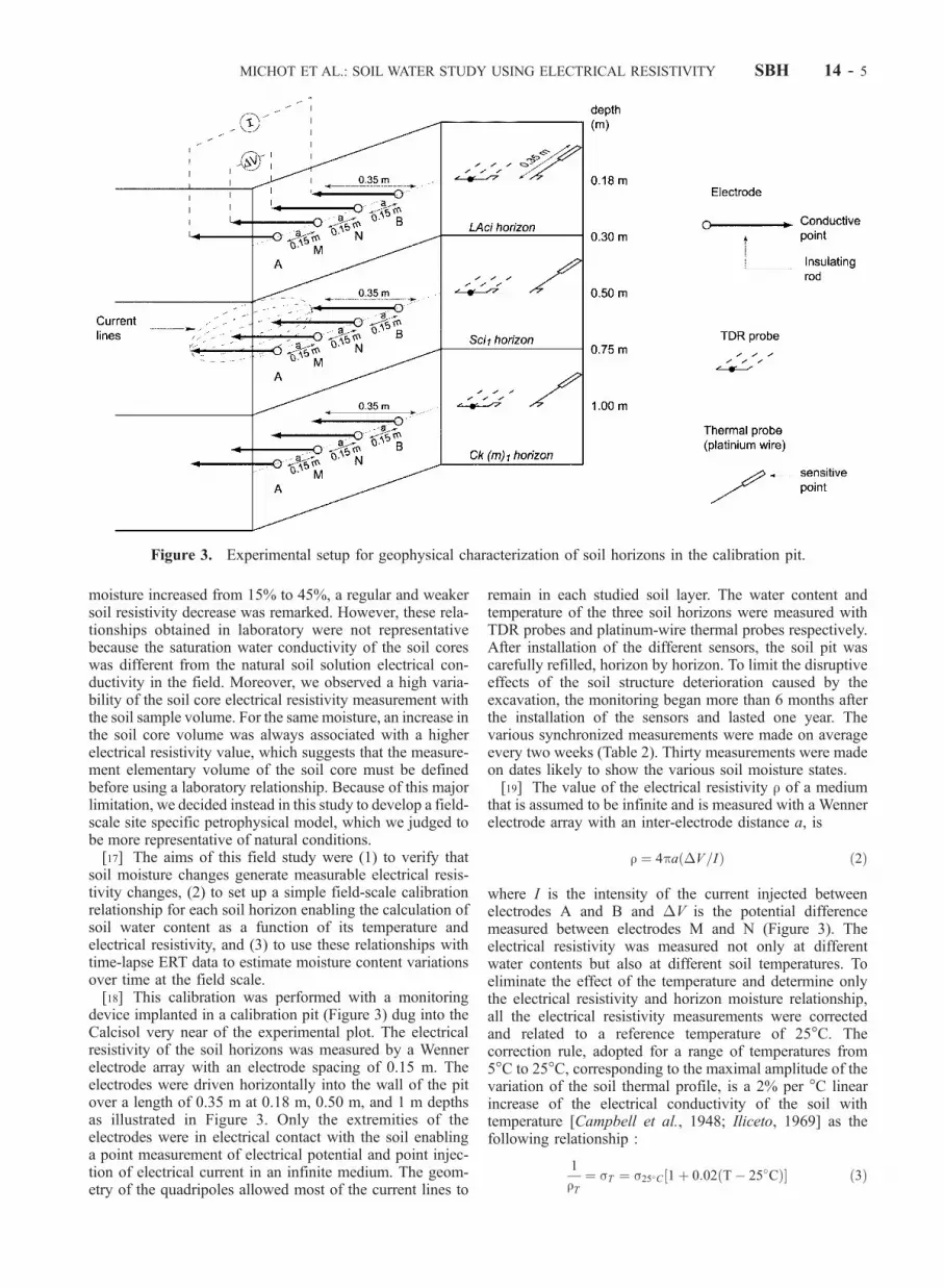
soil moisture changes generate measurable electrical resis-tivity changes, (2) to set up a simple field-scale calibrationrelationship for each soil horizon enabling the calculation ofsoil water content as a function of its temperature andelectrical resistivity, and (3) to use these relationships withtime-lapse ERT data to estimate moisture content variationsover time at the field scale.[18] This calibration was performed with a monitoring

device implanted in a calibration pit (Figure 3) dug into theCalcisol very near of the experimental plot. The electricalresistivity of the soil horizons was measured by a Wennerelectrode array with an electrode spacing of 0.15 m. Theelectrodes were driven horizontally into the wall of the pitover a length of 0.35 m at 0.18 m, 0.50 m, and 1 m depthsas illustrated in Figure 3. Only the extremities of theelectrodes were in electrical contact with the soil enablinga point measurement of electrical potential and point injec-tion of electrical current in an infinite medium. The geom-etry of the quadripoles allowed most of the current lines to

remain in each studied soil layer. The water content andtemperature of the three soil horizons were measured withTDR probes and platinum-wire thermal probes respectively.After installation of the different sensors, the soil pit wascarefully refilled, horizon by horizon. To limit the disruptiveeffects of the soil structure deterioration caused by theexcavation, the monitoring began more than 6 months afterthe installation of the sensors and lasted one year. Thevarious synchronized measurements were made on averageevery two weeks (Table 2). Thirty measurements were madeon dates likely to show the various soil moisture states.[19] The value of the electrical resistivity r of a medium

that is assumed to be infinite and is measured with a Wennerelectrode array with an inter-electrode distance a, is

r ¼ 4pa �V=Ið Þ ð2Þ

where I is the intensity of the current injected betweenelectrodes A and B and �V is the potential differencemeasured between electrodes M and N (Figure 3). Theelectrical resistivity was measured not only at differentwater contents but also at different soil temperatures. Toeliminate the effect of the temperature and determine onlythe electrical resistivity and horizon moisture relationship,all the electrical resistivity measurements were correctedand related to a reference temperature of 25�C. Thecorrection rule, adopted for a range of temperatures from5�C to 25�C, corresponding to the maximal amplitude of thevariation of the soil thermal profile, is a 2% per �C linearincrease of the electrical conductivity of the soil withtemperature [Campbell et al., 1948; Iliceto, 1969] as thefollowing relationship :

1

rT¼ sT ¼ s25�C 1þ 0:02 T� 25�Cð Þ½ ð3Þ

Figure 3. Experimental setup for geophysical characterization of soil horizons in the calibration pit.

MICHOT ET AL.: SOIL WATER STUDY USING ELECTRICAL RESISTIVITY SBH 14 - 5

with rT electrical resistivity at the temperature T (in Celsiusdegree), sT electrical conductivity at the temperature T,s25�C electrical conductivity at 25�C.[20] Linear regression was used to determine the specific

relationships between water content and electrical resistivityof the three typical Calcisol horizons measured in thecalibration pit (Figures 3 and 4). The literature and laboratorymeasurements showed that polynomial function (power 2) orpower function were must commonly used for a large range

of moisture changes ranging between full saturation and drysoil states. However, for low volumetric water contentchanges ranging from 20% to 35% between the permanentwilting point and the field capacity, which corresponds tonatural soil moisture changes in the region, our laboratorymeasurements confirmed that the most simple linear relation-ship was overall sufficient for the all three soil horizons.[21] The relationships between electrical resistivity and

moisture of the three typical horizons of the Calcisol

Table 2. Physical Parameters Measured During Both Monitoring Experiments

Experimentation Experiment Site Experiment TimePhysical Parameters

MeasuredSensors or

Experimental SetupInterval of

Measurement

Spatial and temporalmonitoring of water flow

study area 10 days electrical resistivity r dipole-dipole electricalresistivity tomography

1 hour during a 36 hoursperiod, then irregular

water content q TDR probe 20 minutestemperature T Platinum wire thermal probe 1 hourirrigation water

amountrainfall recorderand rain gauges

continuous measurements

Geophysical characterizationof Calcisol horizons

calibration pit 1 year electrical resistivity r Wenner quadripole 15 days

water content q TDR probe 15 daystemperature T platinum wire thermal probe 15 days

Figure 4. Diagram explaining procedures to monitor spatially and temporally the water flow byelectrical resistivity tomography and to produce a 2-D soil water content tomography.

SBH 14 - 6 MICHOT ET AL.: SOIL WATER STUDY USING ELECTRICAL RESISTIVITY

showed and verified that in the explored domain, electricalresistivity increased linearly with decreasing water content.Nevertheless, the slope and the sensitivity of the relation-ship varied depending on the soil horizon under consider-ation (Figure 5). The linear relation between moisture andelectrical resistivity of the horizons was quantified by theircorrelation coefficient R (Table 3). A quality index j�R/Rjrepresenting the ratio between the confidence interval of thecorrelation coefficient �R for a 5% error margin and thecorrelation coefficient R enabled the relationships to beclassified. When the �R was high and jRj was low, a highindex value showed an inferior quality of the relationship.Inversely, if �R was restricted to a high value of R close to1, a low value of the index indicated a high qualityrelationship.[22] The loamy clay horizon Sci1 displayed the best linear

relationship. The coefficient R, for a confidence level of95%, ranged between the values of �0.98 and �0.92. Thequality index, with a value close to zero, was the lowest ofthe studied soil profiles, which indicated the highest qualitycalibration relationship. The sensitivity, corresponding tothe inverse of the slope absolute value, was 2.8 �m bypercent of soil volumetric water content. Nevertheless, theelectrical resistivity measured was lower than those mea-sured in the laboratory on cylindrical soil cores with the

same moisture range [Michot et al., 2001] and furthermore,the sensitivity of 2.8 �m was clearly higher than thatobserved in the laboratory which was 1.7 �m by percentof soil volumetric water content. This could be explainedeither by a difference between the volume measured in thefield and that of the samples, by the disturbance due to thetransport of the sample in laboratory, or by variability inthe samples.[23] The plowed surface horizon, LAci, displayed a linear

relationship characterized by a coefficient R = �0.80, takenbetween �0.64 and �0.90 for an accepted confidence levelof 95%. The sensitivity of the relationship was 3.9 �m bypercent of soil water content. Considering the data, a power2 polynomial function seemed appropriate too. However, aresidual analysis showed that was not significant improve-

Figure 5. Calibration relationships (T = 25�C) between the moisture and the electrical resistivity ofthree characteristic soil horizons and schematic procedure of 2D soil water content section modelingusing interpreted electrical resistivity model blocks.

Table 3. Summary Statistics to Quantify the Linear Relationship

Between Moisture and Electrical Resistivity of Three Calcisol

Horizons

Soil Horizon n R Rmin Rmax j�R/Rj

LAci 30 �0.80 �0.90 �0.64 0.32Sci1 29 �0.96 �0.98 �0.92 0.06Ck(m)1 30 �0.66 �0.80 �0.39 0.65

MICHOT ET AL.: SOIL WATER STUDY USING ELECTRICAL RESISTIVITY SBH 14 - 7

ment of this curve fitting in comparison with a linearrelationship. Both small range of resistivity and moisturechanges explained that a good fit of such a curve could notbe obtained. On the field, we have not access to soil watercontent extreme values as in laboratory. So, we do not haveany reason to choose a power 2 polynomial function. Alinear relationship was sufficient.[24] The linear relationship observed in the cryoturbated

calcareous horizon of Ck(m)1 presented the lowest correla-tion coefficient and the highest quality index of the threeCalcisol horizons. For a small water content change, theapparent resistivity data were relatively dispersed. Becauseof this major limitation we used only a linear relationship.The heterogeneity of the cryoturbated limestone horizonand the lower moisture variation in this horizon situated at a1 m depth could explain the lower quality of the relation-ship. For a decrease in soil moisture of 5%, the resistivity ofthe horizon increased by 90 �m, i.e. a sensitivity close to19.9 �m by percent of soil volumetric water content.

5. Monitoring

[25] The aim of this field study was to first acquire theresistivity data for later transformation in water content andsecondly, to acquire point water content measurements forvalidation of the estimated water content (Figure 4). For thissecond purpose a second pit was dug near the monitoringstudy area (Figure 2).

[26] This data acquisition was carried out during anirrigation cycle, on a corn crop characterized by a regularimplantation of corn plants in rows justifying a 2-D study.Two-dimensional soil electrical resistivity tomography datawere acquired over time using a multielectrode method at thesurface of the study area. Two-dimensional soil moistureprofiles were then estimated from the 2-D ERT profiles usingthe calibration relationships previously established fromstationary measures in the pit, as described in section 4.[27] Temporal monitoring of the electrical resistivity,

water content and temperature of a vertical soil sectionwas carried out over a period of 10 days (Figure 6 andTable 2), before, during and after irrigation of the exper-imental plot by means of a rotating ramp fitted withsprinklers. Irrigation supplied 25 mm of water by sprinklingon the experimental device between 18h and 20h. On 1September 2000, 5 mm of additional water is supplied byone hour of rainfall. The electrical conductivity of theirrigation water measured in 5 samples taken from 4 raingauges and in the rainfall recorder ranged between 17.510�3 S m�1 and 19 10�3 S m�1 (Table 4).

5.1. Electrical Resistivity Measurementand Interpretation

5.1.1. Electrical Device and Data Acquisition[28] Resistivity measurements were carried out with the

resistivity meter Syscal R1 (Iris Instruments, Orleans,France) equipped with 32 electrodes. The intensity and

Figure 6. Electrical tomography, natural rainfall, and irrigation water depth records over time.

Table 4. Electrical Conductivity of Irrigation Water Samples

Rainfall Recorder

Rain Gauge

1 3 4 5

Sample volume (cm3) 975 550 245 220 495Electrical conductivity (S m�1) 18 � 10�3 19 � 10�3 19 � 10�3 17.5 � 10�3 17.5 � 10�3

SBH 14 - 8 MICHOT ET AL.: SOIL WATER STUDY USING ELECTRICAL RESISTIVITY

voltage accuracy is 0.3%, which is consistent with themeasurements carried out under constant surface conditions.Repeated measurements in stable hydrogeologic conditionsfor about ten hours were persistent within a tenth of an ohm-meter, i.e., one thousandth of the measured resistivity. Duringsprinkling, variations of the measured resistivity could reachseveral ohm-meters between two sets of measurements 1hour apart. The electrodes remained on the soil surface duringall the experiment time to avoid any electrode polarizationchanges and to ensure a best quality of measurements.[29] The experimental setup included a row of 32 elec-

trodes, lined up on the soil surface (Figure 2), in a directionperpendicularly to 8 corn rows, which were separated by 0.8m. This device had a total length of 6.2 m with an electrodespacing (a) of 0.2 m. The dipole-dipole arrangement waschosen because it allowed the greatest number of measure-ments for a given number of electrodes, which was advanta-geous for data inversion. Moreover, the dipole-dipole arraywas very sensitive to horizontal changes in resistivity, butrelatively insensitive to vertical changes in resistivity. Thatmeans that it was convenient in mapping vertical structures,such as water preferential flow direction induced by soilcracks. For each resistivity measurement, electrical currentwas injected between two adjacent electrodes (dipole A B)and the difference potential was measured between twoothers neighboring electrodes (dipole MN). A prepro-grammed measurement sequence (Figure 7) was imple-mented in the resistivity meter and the multiplexerprovided electrode commutation. To obtain the best resolu-

tion, especially down to 0.50 m depth, 345 measurements,located at 15 levels of investigation, were made during eachsequence. The first 6 levels (n) were characterized by aspacing (s = a) between electrodes of each dipole. For eachof these 6 levels (n), the spacing between dipoles was (n� s =n � a). One possible disadvantage of this array was the verysmall signal strength for large values of the (n) factor, thevoltage being inversely proportional to the cube of the (n)factor. This means that for the same current, the voltagemeasured by the resistivity meter dropped by about 200times, when (n) was increased from 1 to 6. One method toovercome this problem, was to increase the (a) spacingbetween both electrodes of each dipole to reduce the dropin the potential when the overall length of the array wasincreased to increase the depth of investigation. So, to insurethe measurement quality at depth with a high signal/noiseratio, 6 new levels (n) were investigated with a spacing (s =2a) between electrodes of each dipole. For the same reason,the measurements at the last 3 levels were made with aspacing (s = 3a). By convention, each apparent electricalresistivity measurements were located at the quadripolecenter and at a depth proportional to both dipole spacing.[30] Each ERT sequence took just under one hour to

acquire. During the first 36 hours of space-time monitoringof the water flow, the resistivity was monitored at regularintervals of 1 hour, then at increasing intervals (Table 2).5.1.2. ERT Processing[31] Inversion of the measured resistivities is an essential

step before interpretation because the raw resistivity mea-

Figure 7. Measurement sequence to construct a pseudosection using a dipole-dipole multielectrodesetup. Measurements are shown on a vertical plane.

MICHOT ET AL.: SOIL WATER STUDY USING ELECTRICAL RESISTIVITY SBH 14 - 9

surements rarely give the true structure of the soil. Pan-issod et al. [2001] showed that the 2-D inversion wasappropriate in this case according to a 3-D inversion.Indeed, a 3-D modeling using both finite difference andmoment-method confirmed the reality of 2-D artifacts,showed that 3-D effects were not significant and allowed usto exclude numerical artifacts. So inverted resistivitysections were achieved with the RES2DINV software [Lokeand Barker, 1996]. This technique was based on thesmoothness-constrained least squares method and it pro-duced 2-D subsurface model from the resistivity section. Inthe first iteration, a homogeneous earth model was used asstarting model for which the resistivity partial derivativevalues could be calculated analytically. For subsequentiterations, a quasi-Newton method was used to estimate thepartial derivatives which reduced the computer time. In thismethod, the Jacobian matrices for a homogeneous earthmodel was used for the first iteration, and the Jacobianmatrices for subsequent iterations were estimated by anupdating technique. The model consisted of a rectangulargrid. The software determined the resistivity of each meshwhich gave a calculated electrical resistivity sectionaccording to field measurements. The iterative optimizationmethod attempted to reduce the differences betweenmeasured resistivity values and those calculated with theinversion model. The difference was estimated by the rootmean square error (RMS error). Topographic correctionwas not taken into account for this inversion process, andeach ERT was inverted independently. The model obtainedfrom the inversion of the initial data set was not used as areference model to constrain the inversion of the later time-lapse data sets, as it was possible with the recent version ofRES2DINV software. A minimum of 5 successiveiterations were made. However, for ERT inversions, thesame number of data and mesh of the model wereconserved, so the inversion of each ERT data was nottotally independent.[32] Each measured resistivity section was inverted.

Water infiltration was indicated by variations in electricalresistivity of the soils, as expected [Ward, 1990], i.e.electrical resistivity in the soils decreases when the soilwater content increases, and vice versa. To enhance therepresentation of that occurrence, sections of resistivitychanges were calculated in relation to some sections mea-sured at typical moments representative of particular hydricsoil states. In this manner of calculating ‘‘differenceimages’’, water infiltration was studied in relation to thefirst ERT (P1, Figure 6) measured at the initial soil moisturestate at the beginning of the experimental monitoring. Soildesiccation by evapotranspiration was observed by compar-ison to an ERT (P37, Figure 6) made after irrigation of a wetsoil, near field capacity, whose moisture profile wastherefore considered stabilized.5.1.3. Procedure for Soil Moisture Estimation UsingERT Data[33] The water content section was shaped from the

rectangular grid network of the 2-D ERT data establishedduring geophysical inversion. The vertical rectangular grid(Figure 5) was composed of 175 rectangular meshes local-ized by their central coordinates (X, Z). X represents thehorizontal distance along the electrode line and Z is thevertical depth of rectangular mesh center. The grid was

divided into 7 layers, which depths were 0.03 m, 0.11 m,0.19 m, 0.30 m, 0.43 m, 0.59 m and 0.80 m respectively.[34] The calibration relationships obtained for the three

typical Calcisol horizons were respectively attributed to thecorresponding rectangular meshes. The relationshipobtained between resistivity and water content of the plowedLAci horizon was used for the first four layers of meshes.The observed relationship on the median structural horizonSci1 was used for the next two layers of meshes. Finally, thetypical relationship of the mineral horizon Ck(m)1 was usedfor the last layer of meshes. As the soil thermal profile wasknown at the moment of each electrical tomography mea-surement, the soil temperature at the center of each mesh wascalculated by linear interpolation. For each one, the calibra-tion relationship for the calculation of water content valueswas selected at the temperature nearest to the real soiltemperature at this depth. The 2-D water content sectionswere then mapped by means of a triangulation method.[35] To evaluate the quality of the soil moisture predic-

tion, 349 water content values measured in the plowed LAcihorizon by TDR probes were compared with those modeledfrom the electrical tomographies measured at the same timeand with the same coordinates (X,Z) (Figure 4). The soilwater contents modeled and compared with the TDRmeasurements were located either under the corn rows(X = 2.7 m and X =3.5 m), or between them (X = 3.1 m andX = 3.9 m). As only the rectangular meshes situated at depthsof Z = 0.1 m, 0.19 m and 0.3 m corresponded to the TDRimplanted at respectively 0.10 m, 0.20 m and 0.30 m depths(Figure 2), the modeled and observed moistures were onlycompared in the plowed LAci horizon. Thus 96, 126, 127moistures content measurements and estimates were com-pared at the respective depths of 0.10 m, 0.20 m and 0.30 m.

5.2. Measurements of Soil Water Content and SoilTemperature Using Conventional Approaches

[36] Soil volumetric water content and soil temperaturewere estimated and measured, simultaneously during ERTacquisition using point measuring devices. Four moistureprofiles were monitored over time using 18 TDR probes.[37] Two moisture profiles were studied directly beneath

a corn row (rows R4 and R5), and two others were locatedbetween two rows (row spacings R4–R5 and R5–R6). TheTDR probes were set at 0.1 m, 0.2 m, 0.3 m, 0.5 m and 0.7m depths in loamy clay horizons. Moisture profiles weremeasured at 20 min intervals. Thermal soil profile changeswere monitored by 5 platinum-wire thermal probes(PT100). Soil temperature was measured at 0.1 m, 0.2 m,0.5 m, 0.7 m and 1 m depths (Figure 2). Thermal profileswere measured every hour (Table 2). At the soil surface, arainfall recorder registered the times and rates of sprinklerirrigation. Five rain gauges measured the amounts ofirrigation water. Two rain gauges were situated underneathcorn rows and three others between corn rows.[38] The distribution on the soil surface of water droplets

from rainfall or sprinkler irrigation depended both on theaerial parts of the corn plants and on the local topography.This topography was the result of farming practices, mainlytractor wheel ruts. Water accumulated on the soil surfaceduring irrigation, formed puddles and water flows along theruts on the slope as streamlets. The rate of water infiltrationinto the soil was therefore lower than the sprinkling rate. In

SBH 14 - 10 MICHOT ET AL.: SOIL WATER STUDY USING ELECTRICAL RESISTIVITY

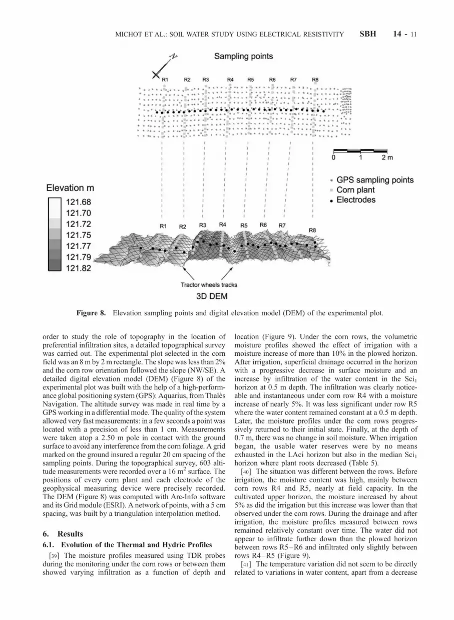
order to study the role of topography in the location ofpreferential infiltration sites, a detailed topographical surveywas carried out. The experimental plot selected in the cornfield was an 8m by 2m rectangle. The slope was less than 2%and the corn row orientation followed the slope (NW/SE). Adetailed digital elevation model (DEM) (Figure 8) of theexperimental plot was built with the help of a high-perform-ance global positioning system (GPS): Aquarius, fromThalesNavigation. The altitude survey was made in real time by aGPSworking in a differential mode. The quality of the systemallowed very fast measurements: in a few seconds a point waslocated with a precision of less than 1 cm. Measurementswere taken atop a 2.50 m pole in contact with the groundsurface to avoid any interference from the corn foliage. A gridmarked on the ground insured a regular 20 cm spacing of thesampling points. During the topographical survey, 603 alti-tude measurements were recorded over a 16 m2 surface. Thepositions of every corn plant and each electrode of thegeophysical measuring device were precisely recorded.The DEM (Figure 8) was computed with Arc-Info softwareand its Grid module (ESRI). A network of points, with a 5 cmspacing, was built by a triangulation interpolation method.

6. Results

6.1. Evolution of the Thermal and Hydric Profiles

[39] The moisture profiles measured using TDR probesduring the monitoring under the corn rows or between themshowed varying infiltration as a function of depth and

location (Figure 9). Under the corn rows, the volumetricmoisture profiles showed the effect of irrigation with amoisture increase of more than 10% in the plowed horizon.After irrigation, superficial drainage occurred in the horizonwith a progressive decrease in surface moisture and anincrease by infiltration of the water content in the Sci1horizon at 0.5 m depth. The infiltration was clearly notice-able and instantaneous under corn row R4 with a moistureincrease of nearly 5%. It was less significant under row R5where the water content remained constant at a 0.5 m depth.Later, the moisture profiles under the corn rows progres-sively returned to their initial state. Finally, at the depth of0.7 m, there was no change in soil moisture. When irrigationbegan, the usable water reserves were by no meansexhausted in the LAci horizon but also in the median Sci1horizon where plant roots decreased (Table 5).[40] The situation was different between the rows. Before

irrigation, the moisture content was high, mainly betweencorn rows R4 and R5, nearly at field capacity. In thecultivated upper horizon, the moisture increased by about5% as did the irrigation but this increase was lower than thatobserved under the corn rows. During the drainage and afterirrigation, the moisture profiles measured between rowsremained relatively constant over time. The water did notappear to infiltrate further down than the plowed horizonbetween rows R5–R6 and infiltrated only slightly betweenrows R4–R5 (Figure 9).[41] The temperature variation did not seem to be directly

related to variations in water content, apart from a decrease

Figure 8. Elevation sampling points and digital elevation model (DEM) of the experimental plot.

MICHOT ET AL.: SOIL WATER STUDY USING ELECTRICAL RESISTIVITY SBH 14 - 11

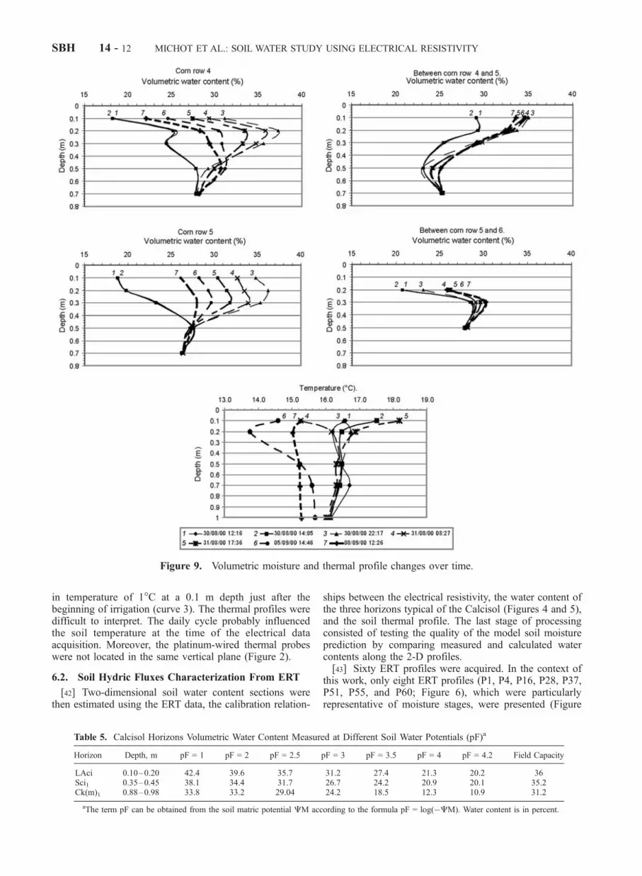
in temperature of 1�C at a 0.1 m depth just after thebeginning of irrigation (curve 3). The thermal profiles weredifficult to interpret. The daily cycle probably influencedthe soil temperature at the time of the electrical dataacquisition. Moreover, the platinum-wired thermal probeswere not located in the same vertical plane (Figure 2).

6.2. Soil Hydric Fluxes Characterization From ERT

[42] Two-dimensional soil water content sections werethen estimated using the ERT data, the calibration relation-

ships between the electrical resistivity, the water content ofthe three horizons typical of the Calcisol (Figures 4 and 5),and the soil thermal profile. The last stage of processingconsisted of testing the quality of the model soil moistureprediction by comparing measured and calculated watercontents along the 2-D profiles.[43] Sixty ERT profiles were acquired. In the context of

this work, only eight ERT profiles (P1, P4, P16, P28, P37,P51, P55, and P60; Figure 6), which were particularlyrepresentative of moisture stages, were presented (Figure

Figure 9. Volumetric moisture and thermal profile changes over time.

Table 5. Calcisol Horizons Volumetric Water Content Measured at Different Soil Water Potentials (pF)a

Horizon Depth, m pF = 1 pF = 2 pF = 2.5 pF = 3 pF = 3.5 pF = 4 pF = 4.2 Field Capacity

LAci 0.10–0.20 42.4 39.6 35.7 31.2 27.4 21.3 20.2 36Sci1 0.35–0.45 38.1 34.4 31.7 26.7 24.2 20.9 20.1 35.2Ck(m)1 0.88–0.98 33.8 33.2 29.04 24.2 18.5 12.3 10.9 31.2

aThe term pF can be obtained from the soil matric potential CM according to the formula pF = log(�CM). Water content is in percent.

SBH 14 - 12 MICHOT ET AL.: SOIL WATER STUDY USING ELECTRICAL RESISTIVITY

10). For each ERT section, two moisture profiles wereindicated. The first moisture profile was obtained just underthe corn row 4, while the second one was measured betweenrows 4 and 5. The section P1, measured at the beginning ofthe experiment, just before irrigation at 12:16 P.M. onAugust 30th, characterized the initial soil moisture statedefined as reference.

6.2.1. Initial Soil Moisture State[44] In the section P1 (first row of Figure 10), the main

typical soil horizons were identified by their electricalresistivity. The first layer between the soil surface and the0.3 m depth corresponded to the plowed LAci loamy-claylayer. It appeared to have a moderate resistivity (20 � m <r < 70 � m), with resistive structures (r > 100 � m) under

Figure 10. Characteristic true soil sections resistivity and volumetric moisture profiles measured overtime during water infiltration after sprinkling and subsequent soil drying phase.

MICHOT ET AL.: SOIL WATER STUDY USING ELECTRICAL RESISTIVITY SBH 14 - 13

each corn plant. According to the profiles of corn rootsdensity (Figure 2) [Nicoullaud et al., 1995], the majorresistivity anomalies in the plowed layer indicated that thesoil volume had dried as a result of corn root water uptake[Michot et al., 2001]. The drying process in the plowedlayer was not uniform. This effect was less intense betweenrows due to compaction by tractor wheels (X-coordinates1.5 and 3.1 m). Soil compaction between the corn rows byagricultural machines was also visible on the DEM(Figure 8). Wheel tracks had modeled the soil microtopo-graphy. The fact that the zones between the corn rows werelower was evidence of their compaction, which was alsoshown by a higher apparent density of the plowed horizonbetween the surface and a depth of 0.1 m (Table 6). Thesecompacted zones had a smaller root density [Tardieu andManichon, 1987]. The systematically oblique variations inthe electrical resistivity of the soil and the obliqueorientation of the pockets of resistant soil within the plowedhorizon seemed linked to the orientation of the plowingclods. However, the obliqueness of these structures couldalso be an artifact linked to the nonsymmetrical positioningof the electrodes in relation to the corn plants or to themeshing of the electrical resistivity section during inversion.[45] The median soil layer corresponding to the Sci1

horizon had the lowest resistivity. The high clay content(32%) of the horizon explained its high conductivity(Table 1). The gradual increase of electrical resistivity withdepth was related to clay content decrease and to smallerwater uptake by corn roots.[46] At a depth of 0.7 to 0.75 m, a resistive layer

appeared, corresponding to the Ck(m)1 horizon composedof beige cryoturbated limestone.6.2.2. Water Infiltration Phase[47] After irrigation, monitoring of the water flows was

performed using the relative variations of ERT sections(Figure 11). Before irrigation, the electrical tomographiesP1 and P4 measured at a two-hour interval in the samemoisture conditions produced closely comparable resistiv-ities. In the absence of change in the moisture state of thesoil, in particular at the greatest depths, the electricalresistivity measurements were reproduced.[48] During the moistening phase after the application of

25 mm of sprinkled water, the progressive saturation of theplowed LAci horizon by infiltration explained the generaldecrease in soil resistivity.[49] Selective infiltration occurred under the corn plants

and not in the low zones, between the corn rows, wheresurface water had a tendency to accumulate due to the effectof the soil microtopography (Figures 8 and 11). The verticalanomalies of negative electrical resistivity changes observedunder the corn rows corresponded to the preferential direc-tions of water flow. The aerial parts of the corn plantsplayed an important role in the catching of water droplets.The water ran down the length of the stem, causing first anincrease in soil moisture, and then infiltration under the cornplants. The role of topography would therefore appear to beless important in water infiltration as the water hardlyinfiltrated in the low zones between the rows.[50] Three resistive pockets in the LAci horizon between

corn rows R3 and R4 persisted over time. This wasexplained by the local soil microtopography. The irrigationwater did not infiltrate here but ran rapidly in the direction

of the slope toward the low zones in the soil surface createdby tractor-wheel tracks (Figure 8).[51] Locally, the upper parts of the median Sci1 horizon

showed resistivities of less than 20 � m, with a 20 to 70%resistivity decrease compared to the initial soil conditions.The percolating water could reach the upper part of thehorizon and accumulated in the pores of the horizon.[52] Two vertical structures located between two corn

rows were characterized by an electrical resistivity that wasconstant or slightly increased over time. These domainswere separated by a distance of 1.6 m to 1.8 m, correspond-ing to wheel span of an agricultural machine. The base ofthe LAci horizon was probably compacted by the passage ofan agricultural machine before the corn was sown as thewheel tracks corresponding to the compacted zones did notappear in the soil topography. Soil compaction was shownbetween corn rows R5 and R6 by a higher bulk density ofthe LAci horizon, which could reach a value of 1.56 (Table6). Compaction of the plowed horizon by the wheels ofagricultural machines significantly reduced the infiltrationcapacity of the soil. Ankeny et al. [1990] showed thatthe hydraulic conductivity of the soil was greatly reduced bythe passage of the wheels and they attributed this to thedestruction of the macropores by compaction. The compact-ing of the horizon could create a shadow zone preventingthe vertical infiltration of the water. Similarly, water wascollected between the rows and was evacuated down theslope as runoff. There were two possible explanations ofsoil electrical resistivity increase either a soil temperaturedecrease or a soil moisture decrease. However, a numericalsimulation showed that a realistic soil temperature decreaseof 1�C provoked by cold water infiltration nearby could notexplain an electrical resistivity increase higher than 5%. Atthe same depth, the soil moisture changes under a corn plantcould be very different and even inverse from thoseobserved under the both compacted area because the waterinfiltrated to this depth with different velocities. Moreover,the soil moisture history could involve different hydricbehaviors. The experiment performed a sudden soilmoistening after a slow drying phase between two watersprinklings. Under the compacted horizon characterized bya low hydraulic conductivity the local wetting kinetic wasasynchronous in comparison with the rest of the soil profile.Both these domains were always in a slow drying phase. So,the electrical resistivity increase could be explained by alocal water content decrease.6.2.3. Soil Desiccation Phase[53] During the drying phase, after the drainage period,

the soil pockets characterized by a high electrical resistivity

Table 6. Bulk Density (da) of Ploughed LAci Horizon Measured

on Cylindrical Soil Cores Sampled Between the Soil Surface and

0.1 m Deptha

Location da 1 da 2 da 3 MeanStandardDeviation

Corn row R4 1.28 1.23 1.26 1.26 0.03Between corn rows R4-R5 1.52 1.58 1.37 1.49 0.11Corn row R5 1.27 1.19 1.26 1.24 0.04Between corn rows R5–R6 1.56 1.30 1.34 1.40 0.14

aSoil core volume is 500 cm3.

SBH 14 - 14 MICHOT ET AL.: SOIL WATER STUDY USING ELECTRICAL RESISTIVITY

Figure

11.

Soilsectionsofrelativeresistivitychanges

measuredover

timerespectivelyduringthesoilwettingphaseand

subsequentdryingphase.

MICHOT ET AL.: SOIL WATER STUDY USING ELECTRICAL RESISTIVITY SBH 14 - 15

reappeared under the corn plants in the LAci horizon(Figure 11). The size of the structures associated with thepositive variations in electrical resistivity in relation to theelectrical tomography P37 increased with time. The increasein electrical resistivity was first seen in the LAci horizon,

then spread progressively downward. Soil pockets, drainedby the corn root water uptake, were detected by an increasein the electrical resistivity of the soil. At the end of themonitoring period, the shape of the positive resistivityanomalies under the corn plants and the amplitude of the

Figure 12. Characteristic soil moisture content sections computed over time during the experimentalmonitoring period.

SBH 14 - 16 MICHOT ET AL.: SOIL WATER STUDY USING ELECTRICAL RESISTIVITY

increase in electrical resistivity, evolved in the same way asthe corn root frequency profiles : higher in the plowedhorizon and lower at depth [Nicoullaud et al., 1995]. Tostrengthen these observations and to retrieve informationabout root water uptake and soil water reserve from the timevariations of resistivity, Tabbagh et al. [2002] havedeveloped a model that solves simultaneously Richard’sand heat conduction equations, and delivers for each timeintervals the soil water distribution after sprinkling and thecorresponding resistivity variations.

6.3. Soil Moisture Sections and Validation

[54] Five 2-D sections of moisture content of the selectedsoil, estimated using the ERT data obtained at various datesof the monitoring, are presented in Figure 12. The use of alinear relationship between moisture and electrical resistiv-ity for the three soil horizons suggests that the spatialstructure of the moisture sections and of the electricalresistivity sections are similar. The moisture sections repro-duce the water flow previously revealed by variations inelectrical resistivity during the phases of water infiltrationand soil drainage.[55] For the whole of the plowed LAci horizon, the water

contents estimated using ERT data are effectively correlated

with the measured values (R = 0.68) using TDR data (Figure13 and Table 7). The slope of the linear regression betweenthe modeled and measured water contents is close to theideal value of 1. The estimate precision was quantified by theroot mean square error (RMSE), while the estimation biaswas quantified by the mean error (ME). The estimation biasis small and corresponds to an overestimation of 1.45% ofthe volumetric moisture. The precision of the water contentestimation is 3.63%. The residual histogram, correspondingto the difference between the measured and calculatedmoistures, shows a Gaussian distribution of the residues(Figure 14). The histogram also shows that 26.5% ofthe residues range between �1% and +1% of volumetric

Figure 13. Validation: relationship between the moisture content of the ploughed horizon established by2-D tomography and soil water content measured with TDR probes at the same time and the samelocation.

Table 7. Summary Statistics to Compare Soil Volumetric Water

Content Estimated From Electrical Resistivity Tomography and

That Measured With TDR Probes

Depth, m n R ME, % RMSE, %

0.1 to 0.3 349 0.68 �1.45 3.630.1 96 0.75 �1.59 3.850.2 126 0.76 �0.38 3.260.3 127 0.45 �2.40 3.80

MICHOT ET AL.: SOIL WATER STUDY USING ELECTRICAL RESISTIVITY SBH 14 - 17

moisture and that 67% of the residues are between �3% and+3% of volumetric moisture. The quality of the estimate ofsoil moisture is therefore satisfying.[56] In Table 7, the highest correlation coefficient, the

smallest bias and the greatest precision, reveal the bestmoisture estimation at a depth of 0.2 m.[57] Conversely, at a depth of 0.3 m the correlation

coefficient between the calculated and measured moisturesis the lowest, the estimation bias the highest and theestimation precision the worst. At this depth, the moistureseems slightly overestimated as the majority of the estima-tion residues (33%) is between �3% and �1% of volu-metric water content. The presence of the plowed pan at adepth of 0.3 m may explain this low correlation. Theplowed pan constitutes the limit between the plowed surfacehorizon and the structural horizon Sci1. At this level, thestructure of the LAci horizon compacted by tillage ismodified. The plowed pan is characterized by a majordecrease in porosity and a modification of the hydrody-namic behavior of the horizon with a reduced infiltration.These changes explain why the calibration relationship ofthe LAci horizon is less adapted at this level and thereforewhy the correlation is lower.[58] Several factors may explain the deviation between the

soil water content estimation using ERTand measured by the

TDR probes. (1) One is the distance of about 1 m separatingthe multielectrode device from the TDR profiles while soilmoisture varies on a decimeter scale. (2) Another is the effectof the sides of the trench on the water flow. (3) The differ-ence between the soil resistivity during the monitoring andthe resistivity calculated by the 2-D ERT inversion procedureis another factor. The precision of the inversion and thereforeof the estimation of the soil resistivity depends, among othersources of uncertainties, on the configuration of the electro-des, the interval between the electrodes and the number ofmeasurements of the apparent resistivity of the soil. (4)Although small electrodes were used to reduce the contactresistance between the soil and the electrode, it is difficult toconsider them as points which would be necessary forsurveys requiring high resolution and shallow investigationdepths. (5) The resistivity of soils may be subject tohysteretic phenomena. (6) As the conduction of current insoils is mainly electrolytic, soil resistivity depends not onlyon moisture and temperature but also on the ionic concen-tration of the studied soil solutions. During the experiment,the soil solution may be diluted by irrigation water pumpedinto a stratified aquifer with a significant TDS loading[Schnebelen et al., 1999] leading to nonnegligible variationsin the electrical resistivities. (7) The time (1 hour) needed toacquire a resistivity section is relatively long compared with

Figure 14. Residue frequency histograms between the ploughed horizon water content measured byTDR probes and soil water content estimated from electrical resistivity tomography measured at the sametime and the same location.

SBH 14 - 18 MICHOT ET AL.: SOIL WATER STUDY USING ELECTRICAL RESISTIVITY

the infiltration rate of water during irrigation. A devicepermitting more rapid data collection must be considered inthe future.

7. Conclusions

[59] Acquiring ERT data along a vertical soil section witha multielectrode surface method, which is nondestructiveand spatially integrating, the boundaries of some soilhorizons were delineated. Soil moisture changes over timewere revealed by electrical resistivity changes in the soil.Two-dimensional soil water content sections were calcu-lated from the ERT using field-scale calibration relation-ships between the electrical resistivity of each soil horizonand its water content. As the temperature variations in thesoil affect the electrical resistivity of the water and thereforethat of the soil, the thermal profile of the soil during theelectrical resistivity measurements were taken into accountin the calculation. A comparison of the modeled watercontents with those measured by TDR probes confirmedthat the reliability of a site-specific linear relationshipbetween the calculated and measured moistures in theplowed LAci surface horizon. Overall, in the plowed sur-face horizon, the moisture estimates showed a precision of3.6% for an estimation bias corresponding to a watercontent overestimation of 1.4%. The best estimation wasobtained at 20 cm depth where the effects of both largesurface moisture fluctuations and compaction of the plowedpan were attenuated.[60] The hydraulic functioning of the soil was then

monitored during a moistening/drying cycle. The dryingout of the soil by corn root water uptake, the progression ofthe infiltration front after irrigation, the delimitation ofpreferential-flow zones and the surface drainage of the soilwere identified and localized. At this stage of corn develop-ment (3 months), the parts of the soil involved in soilinfiltration and drainage were mainly located directly underthe corn rows. The corn plants played a major role in theredistribution of surface water before it infiltrated, while therole of the topography in water infiltration appeared to belimited. The particular structural characteristics of the soilhorizons resulting from agricultural practices, and the nota-ble effect of soil compaction due to the passage of agricul-tural machines were observed. In zones where the soil wascompacted, moisture variations were negligible, whichdemonstrated the negative effects of compaction on waterflow as well as on the possibilities of water storage.[61] Measurements of soil water content using conven-

tional tools typically sampling over small volumes, at wideintervals, and in an intrusive manner, are generally lessrepresentative than the actual and very complex situation ofthe soil moisture state. They do not allow a good monitoringof the evolution of soil moisture. Estimation of watercontent using ERT as a first approximation of the spatialdistribution of soil water content in a cultivated soil isshown to be significant. Nevertheless, the validity of theproposed model could be limited to specific regional con-ditions such as loamy clay soils of the Beauce region.[62] In the future, this method may allow verification of

sprinkling irrigation efficiency and better estimation of theuseful available water in the soil. Water spatial distributionis influenced by crop root distribution with depth, which isdependent on soil type and soil management as tillage

operations. This method is a high-resolution investigationtool to study soil moisture and to perform soil water flowtemporal monitoring.[63] The development and adoption of precision farming

and rational irrigation require a detailed knowledge of soilsand crops [Robert, 1999]. This method is useful in researchto describe the soil spatial variability and its hydric behaviorwith a high resolution. However, the precision is higher thanthe investigation level required in precision farming, and therequirement of an additional field calibration may render themethod impractical for routine field use. The use of ageneral petrophysical relationship between the soil electricalresistivity and its moisture, if appropriate, could reduce theeffort needed to make this a practical field tool for thepurpose of improving irrigation management.

[64] Acknowledgment. We are grateful to the Associate Editor and tothe anonymous reviewers for their constructive comments.

ReferencesAaltonen, J., Seasonal changes of DC resistivity measurements, paper pre-sented at 3rd EEGS-ES Conference, Environ. and Eng. Geophys. Soc.,Aarhus, Denmark, 1997.

Amin, M. H. G., R. J. Chorley, K. S. Richards, B. W. Bache, L. D. Hall, andT. A. Carpenter, Spatial and temporal mapping of water in soil by mag-netic resonance imaging, Hydrol. Processes, 7, 279–286, 1993.

Ankeny, M. D., M. Ahmed, T. C. Kaspar, and R. Horton, Characterizationof tillage and traffic effects on unconfined infiltration measurements, SoilSci. Soc. Am. J., 54, 837–840, 1990.

Archie, G. E., The electrical resistivity log as an aid in determining somereservoir characteristics, Trans. Am. Inst. Min. Metall. Pet. Eng., 146,54–67, 1942.

Baize, D., and M. C. Girard, Solums carbonates et satures, in ReferentielPedologique, pp. 109–120, INRA Ed., Paris, 1995.

Barker, R., and J. Moore, The application of time lapse electrical tomogra-phy in ground water studies, Leading Edge, 17, 1454–1458, 1998.

Barraud, J. P., A. Dieulin, E. Ledoux, and G. de Marsily, Relation entremesures geophysiques et flux de l’eau dans les sols non satures, Rapp.LHM/RD/79/3, Ecole Natl. Superieure des Mines de Paris, Paris, 1979.

Bavel, C. H. M., N. Underwood, and R. W. Swanson, Soil moisture mea-surement by neutron moderation, Soil Sci., 82, 29–41, 1956.

Beauce, A., J. Bernard, A. Legchenko, and P. Valla, Une nouvelle methodegeophysique pour les etudes hydrogeologiques: L’application de la reso-nance magnetique nucleaire, Hydrogeologie, 1, 71–77, 1996.

Bell, J. P., T. J. Dean, and M. G. Hodnett, Soil moisture measurement by animproved capacitance technique, part II. Field techniques, evaluation andcalibration, J. Hydrol., 93, 79–90, 1987.

Benderitter, Y., and J. J. Schott, Short time variation of the resistivity in anunsaturated soil: The relationship with rainfall, Eur. J. Environ. Eng.Geophys., 4, 37–49, 1999.

Binley, A., P. Winship, R. Middleton, M. Pokar, and J. West, Observationsof seasonal dynamics in the vadose zone using borehole radar andresistivity, paper presented at the Annual Symposium on the Applicationof Geophysics to Engineering and Environnemental Problems (SA-GEEP), Environ. and Eng. Geophys. Soc., Denver, Colo., 2001.

Bussian, A. E., Electrical conductance in a porous medium, Geophysics, 48,1258–1268, 1983.

Campbell, R. B., C. A. Bower, and L. A. Richards, Change of electricalconductivity with temperature and the relation of osmotic pressure toelectrical conductivity and ion concentration for soil extracts, Soil Sci.Soc. Am. Proc., 13, 66–69, 1948.

Chanasyk, D. S., and M. A. Naeth, Field measurement of soil moistureusing neutron probes, Can. J. Soil Sci, 76, 317–323, 1996.

Clavier, C., G. Coates, and J. Dumanoir, The theorical and experimentalbases for the ‘‘Dual water’’ model for the interpretation of shaly sands,paper presented at 52nd Annual Fall Technical Conference and Exhibi-tion of the SPE of AIME, Am. Inst. of Mining, Metall., and Pet. Eng.,Denver, Colo., 9 –12 Oct. 1977.

Cosentino, P., A. Cimino, and A. M. Riggio, Time variations of the resis-tivity in a layered structure with unconfined aquifer, Geoexploration, 17,11–17, 1979.

MICHOT ET AL.: SOIL WATER STUDY USING ELECTRICAL RESISTIVITY SBH 14 - 19

Daily, W., and A. Ramirez, Evaluation of electromagnetic tomography tomap in situ water in heated welded tuff, Water Resour. Res., 25, 1083–1096, 1989.

Davis, J. L., and A. P. Annam, Ground penetrating radar for high resolutionmapping of soil and rock stratigraphy, Geophys. Prospect., 37, 531–551,1989.

Dean, T. J., J. P. Bell, and A. J. B. Baty, Soil moisture measurement by animproved capacitance technique, part I, Sensor design and performance,J. Hydrol., 93, 67–68, 1987.

Eppstein, M. J., and D. E. Dougherty, Efficient three-dimensional datainversion: Soil characterization and moisture monitoring from cross-wellground-penetrating radar at a Vermont test site, Water Resour. Res., 34,1889–1900, 1998.

Flury, M., H. Fluhler, W. A. Jury, and J. Leuenberger, Susceptibility of soilsto preferential flow of water: A field study, Water Resour. Res., 30,1945–1954, 1994.

Gardner, W., and D. Kirkham, Determination of soil moisture by neutronscattering, Soil Sci., 73, 391–401, 1952.

Goldman, M., B. Rabinovich, M. Rabinovich, D. Gilad, I. Gev, andM. Schirov, Application of the integrated NMR-TDEM method ingroundwater exploration in Israel, J. Appl. Geophys., 31, 27–52, 1994.

Griffiths, D. H., and R. D. Barker, Two-dimensional resistivity imaging andmodeling in areas of complex geology, J. Appl. Geophys., 29, 211–226,1993.

Griffiths, D. H., and J. Turnbull, A multi-electrode array for resistivitysurveying, First Break, 3, 16–20, 1985.

Griffiths, D. H., J. Turnbull, and A. I. Olayinka, Two-dimensional resistivitymappingwith a computer controlled array,First Break, 8, 121–129, 1990.

Hagrey, S. A., and J. Michaelsen, Resistivity and percolation study ofpreferential flow in vadose zone at Bokhorst, Germany, Geophysics,64, 746–753, 1999.

Heimovaara, T. J., and W. Bouten, A computer-controlled 36-channel timedomain reflectometry system for monitoring soil water contents, WaterResour. Res., 26, 2311–2316, 1990.

Herkelrath, W. N., S. P. Hamburg, and F. Murphy, Automatic, real-timemonitoring of soil moisture in a remote field area with time domainreflectometry, Water Resour. Res., 27, 857–864, 1991.

Hubbard, S. S., Y. Rubin, and E. Majer, Ground-penetrating radar assistedsaturation and permeability estimation in bimodal systems,Water Resour.Res., 33, 971–990, 1997.

Hubbard, S. S., K. Grote, and Y. Rubin, Mapping the volumetric soil watercontent of a California vineyard using high-frequency GPR ground wavedata, Leading Edge, 21, 552–559, 2002.

Huisman, J. A., C. Sperl, W. Bouten, and J. M. Verstraten, Soil watercontent measurements at different scales: Accuracy of time domain re-flectometry and ground-penetrating radar, J. Hydrol., 245, 48–58, 2001.

Iliceto, V., Contribution a la prospection geophysique des sites archeologi-ques, Ph.D. thesis, Univ. de Paris, Paris, 1969.

Isambert, M., and O. Duval, Notice explicative de la carte pedologique deVillamblain (Beauce) au 1/10000eme, contrat de recherche site experi-mental de Villamblain, rapport periode 1991 –1992, 38 pp., Serv.d’Etude des Sols et de la Carte Pedol. de France, Ardon, 1992.

Kung, K. J. S., Preferential flow in a sandy vadose zone: I Field observa-tion, Geoderma, 46, 51–58, 1990a.

Kung, K. J. S., Preferential flow in a sandy vadose zone: II Mechanism andimplication, Geoderma, 46, 59–71, 1990b.

Loke, M. H., and R. D. Barker, Rapid least-squares inversion of apparentresistivity pseudosections using a quasi-Newton method, Geophy. Pro-spect., 44, 131–152, 1996.

Michot, D., A. Dorigny, and Y. Benderitter, Mise en evidence par resistiviteelectrique des ecoulements preferentiels et de l’assechement par le maısd’un Calcisol de Beauce irrigue, C. R. Acad. Sc. Paris, Serie Iia, 332,29–36, 2001.

Mualem, Y., and S. P. Friedman, Theoretical prediction of electrical con-ductivity in saturated and unsaturated soil, Water Resour. Res., 27,2771–2777, 1991.

Nicoullaud, B., R. Darthout, and O. Duval, Etude de l’enracinement du bletendre d’hiver et du maıs dans les sols argilo-limoneux de Petite Beauce,Etude et Gestion des Sols, 2, 183–200, 1995.

Nicoullaud, B., O. Duval, M. Eimberck, A. Dorigny, and M. Isambert,Cartographie pedologique, Aspects sur le terrain, Livret guide, Organisa-tion de la couverture pedologique et modelisation des processus spatiaux,Journees de formation jeunes chercheurs, 26 –30/05/1997, Orleans.INRA, Departement de Science du Sol., 34 pp., 1997.

Panissod, C., D. Michot, Y. Benderitter, and A. Tabbagh, On the effective-ness of 2D electrical inversion results: An agricultural case study, Geo-physical Prospecting, 49, 570–576, 2001.

Park, S., Fluid migration in the vadose zone from 3-D inversion of resis-tivity monitoring data, Geophysics, 63, 41–51, 1998.

Parkin, G., D. Redman, P. V. Bertoldi, and Z. Zhang, Measurement of soilwater content below a wastewater trench using ground-penetrating radar,Water Resour. Res., 36, 2147–2154, 2000.

Revil, A., L. M. Cathles III, S. Losh, and J. A. Nunn, Electrical conductiv-ity in shaly sands with geophysical applications, J. of Geophysical. Re-search., 103, 23,925–23,936, 1998.

Ritsema, C. J., and L. W. Dekker, How water moves in a water repellentsandy soil, 2, Dynamics of fingered flow, Water Resour. Res., 30, 2519–2531, 1994.

Ritsema, C. J., L. W. Dekker, J. M. H. Hendrickx, and W. Hamminga,Preferential flow mechanism in water repellent sandy soil, Water Resour.Res., 29, 2183–2193, 1993.

Robert, P. C., Precision agriculture: Research needs and status in the USA,2nd European Conference on Precision Agriculture, Odense, Denmark,11–15 July, 19–34,1999.

Rothe, A., W. Weis, K. Kreutzer, D. Matthies, U. Hess, and B. Ansorge,Changes in soil structure caused by the installation of time domainreflectometry probes and their influence on the measurement of soilmoisture, Water Resour. Res., 33, 1585–1593, 1997.

Scanlon, B. R., and R. S. Goldsmith, Field study of spatial variability inunsaturated flow beneath and adjacent to playas, Water Resour. Res., 33,2239–2252, 1997.

Schnebelen, N., E. Ledoux, A. Bruand, and G. Creuzot, Stratificationhydrogeochimique et ecoulements verticaux dans l’aquifere des Cal-caires de Beauce (France): Un systeme anthropise a forte variabilitespatiale et temporelle, C. R. Acad. Sci. Paris, Ser. IIa, 329, 421–428,1999.

Sheets, K. R., and J. M. H. Hendrickx, Non-invasive soil water contentmeasurement using electromagnetic induction, Water Resour. Res., 31,2401–2409, 1995.

Shima, H., Two dimensional automatic resistivity inversion technique usingalpha centers, Geophysics, 55, 682–694, 1990.

Tabbagh, A., Y. Benderitter, D. Michot, and C. Panissod, Measurement ofvariations in soil electrical resistivity for assessing the volume affectedby plant water uptake, Eur. J. Environ. Eng. Geophys., 7, 229–237,2002.

Tardieu, F., and H. Manichon, I-Etat structural, enracinement et alimenta-tion hydrique du maıs, II-Croissance et disposition spatiale du systemeracinaire, Agronomie, 7, 201–211, 1987.

Topp, G. C. and J. L. Davis, Time-domain reflectometry (TDR) and itsapplication to irrigation scheduling, in Advances in Irrigation, vol. 3,edited by D. Hillel, pp. 107–127, Academic, San Diego, Calif., 1985.

Topp, G. C., J. L. Davis, and A. P. Annan, Electromagnetic determination ofsoil water content, Measurements in coaxial transmission lines, WaterResour. Res., 16, 574–582, 1980.

Ward, S. H., Resistivity and induced polarisation methods, in Geotechnicaland Environmental Geophysics, vol. 1, edited by S. H. Ward, pp. 147–189, Soc. of Exp. Geophys., Tulsa, Okla., 1990.

Waxman, M. H., and L. J. M. Smits, Electrical conductivities in oil-bearingshaly sand, Soc. Pet. Eng. J., 8, 107–122, 1968.

Weiler, K. W., T. S. Steenhuis, J. Boll, and K. J. S. Kung, Comparison ofground penetrating radar and time domain reflectometry as soil watersensors, Soil Sci. Soc. Am. J., 62, 1237–1239, 1998.

White, P. A., Electrode arrays for measuring groundwater flow directionand velocity, Geophysics, 59, 192–201, 1994.

Worthington, P. F., The evolution of shaly sand concepts in reservoir eva-luation, Log Anal., 26, 23–40, 1985.

Wyllie, M. R. J., and P. F. Southwick, An experimental investigation of theS. P. and resistivity phenomena in dirty sands, J. Pet. Technol., 6, 44–57,1954.

Zhang, J., R. L. Mackie, and T. R. Madden, 3-D resistivity forward model-ing and inversion using conjugate gradients, Geophysics, 60, 1313–1325, 1995.

Zhou, Q. Y., J. Shimada, and A. Sato, Three-dimensional spatial and tem-poral monitoring of soil water content using electrical resistivity tomo-graphy, Water Resour. Res., 37, 273–285, 2001.

����������������������������Y. Benderitter and A. Tabbagh, UMR 7619 ‘‘Sisyphe’’, UMPC, CNRS,

case 105, 4 Place Jussieu, 75252 Paris Cedex 05, France.A. Dorigny, D. King, D. Michot, and B. Nicoullaud, Institut National de

la Recherche Agronomique Orleans, Unite de Science du Sol, BP 20619,45166 Olivet Cedex, France. (didier.michot@orleans.inra.fr)

SBH 14 - 20 MICHOT ET AL.: SOIL WATER STUDY USING ELECTRICAL RESISTIVITY