Style drift, fund flow and fund performance:new cross-sectional evidence

Kathryn A. Holmes, Robert W. Faff*

Department of Accounting and Finance, Monash University, Victoria 3800, Australia

Abstract

The linkages between style change, fund flows, fund size, and resulting fund performance arecomplex and not clearly understood. In this paper, we investigate these relationships using a sampleof Australian multisector trusts over the sample period 1990 to 1999. We employ a range of fundperformance measures of stock selectivity. We find that levels of style drift are positively related toselectivity performance, but are not related to fund flows. We also find that fund size is positivelyrelated to fund performance and negatively related to expense ratios. Implications of our findings forinvestors are identified in the paper. © 2007 Academy of Financial Services. All rights reserved.

JEL classification: G23; G21; G10

Keywords: Style drift; Fund flows; Managed fund performance; Returns-based style analysis

1. Introduction

The style of many managed funds drift or even change over time (Brown & Goetzmann,1997; Chan, Chen & Lakonishok, 2002; Kim, Shukla & Thomas, 2000; Swinkels & Van DerSluis, 2001). Although some style changes might be caused inadvertently because ofunrelated manager decisions, there is some evidence that funds might deliberately changestyles to attract new fund flow. In a notable recent example, Cooper, Gulen and Rau (2005)find that a style change in a fund’s name can attract significantly abnormal flow in the monthsafter the change. They suggest that funds might time ‘style’ changes to exploit investor

* Corresponding author. Tel.: �61-3-9905-2387; fax: �61-3-9905-2339.E-mail address: Robert.Faff@buseco.monash.edu.au (R. Faff).

Financial Services Review 16 (2007) 55–71

1057-0810/07/$ – see front matter © 2007 Academy of Financial Services. All rights reserved.

irrationality. Alternatively, a change in style often occurs after a management change (Gallo& Lockwood, 1999) and as such might not be intended by design.

One factor that is frequently discussed in relation to fund style drift is the degree to whichfund flows can influence managerial decisions that subsequently result in style changes. Inthe current paper, using a sample of Australian multisector managed funds, we examine thelinks between fund flow and style drift, controlling for other factors that might affect fundperformance; for example, fund size, fund category, and management expense ratios(MER).1 The potential motives for possible style change in the Australian managed fundmarket are very similar to those put forward in the United States setting. The most potentforce is likely to be the way in which many managers receive their compensation: as apercentage of funds under management. In Australia, this practice is most likely to beapplicable to domestic equity managers.2

Why should individual investors care about style drift and its potential relation to fundperformance? One answer to this question relates to the manner in which many investors canpractically eliminate from consideration large numbers of funds from the many thousandscontained in the fund universe, to reduce their choice to more manageable proportions. Putsimply, faced with information overload, the category to which funds are assigned representsan attractive and expedient screening device for investors. By assessing their personal goalsand tolerance for risk, individual investors can isolate a smaller group of potentially suitablefunds according to the stated objective that each fund makes public via their prospectus (andother publicity or advertising). If fund managers do not strictly comply with their statedobjective (whether by design or simply by inferior or slack practices), over time their actualstyle might be materially different from what it should be. Individual investors could easilybe exposed to risk levels or types that are largely incompatible with their own personalsituations, thereby creating a less than satisfactory investment experience. In the extremescenario, this could lead to grossly inferior performance to that which they were expectingbased on stated fund objectives. More subtly, even if the performance is not wildly differentfrom (or even superior to) expectations, it may have been achieved with a very different riskprofile than investors would prefer. As such, the individual investor should be acutelyinterested in the general issue of style drift and more particularly how fund performancerelates to style drift. Accordingly, our goal is to shed light on this basic research question.

We use a range of fund performance measures of stock selectivity. We begin by estimatingalphas using the standard performance models, such as Jensen and Treynor–Mazuy, alongwith a cubic market model, which allows volatility timing to be considered in the model.Second, as there are suggestions in the literature that the inclusion of public informationvariables provides a more reliable measure of fund performance (Holmes & Faff, 2004;Sawicki & Ong, 2000), we also incorporate conditional variables in the Treynor–Mazuymodel. Third, the standard and conditional models apply restrictions to the level of fund risk.To relax this constraint, we also examine the alpha measures arising from an application ofthe Kalman filter, allowing fund risk to vary via a random walk.

Our findings can be summarized as follows. Based on rolling returns-based style analysis,we demonstrate a relatively high incidence of style drift, which for some funds in the sampletakes on the appearance of major style change. Although we do not find support for a stronglink between fund flow and style drift, we do find that style drift is related to fund

56 K.A. Holmes, R.W. Faff / Financial Services Review 16 (2007) 55–71

performance. Specifically, we find evidence that style drift and selectivity are positivelyrelated.

The remainder of the paper is organized as follows. In Section 2, we review the literaturedealing with fund flow, style drift and fund size, focusing on the relationship of thesevariables to fund selectivity performance. In Section 3, the research method is detailed,whereas Section 4 briefly describes the data. In Section 5, the results are discussed andconclusions are reached in Section 6.

2. Literature review

2.1. Fund flow

This cyclic relationship between flows, style drift, and performance is problematic tounderstand. Significant amounts of new flow could cause a manager to trade more frequently,therefore incurring more transaction costs. In addition, fund flows can constrain a fundmanager from adhering to an optimal investment strategy, as they might have to hold morecash to allow for erratic flows (Edelen, 1999; Rakowski, 2003). Negative tax implicationsmight also arise from significant fund flows (Shoven, Dickson & Sialm, 2000). In addition,a fund demonstrating style inconsistency could discourage further investment and, therefore,result in fund outflows. Cooper et al. (2005) find that a change in the style of the name ofa fund can subsequently attract significant amounts of fund flow.

Many studies have examined the relationship between fund flows and performance (Berk& Green, 2004; Chevalier & Ellison, 1997; Deaves, 2004; DelGuercio & Tkac, 2002; Sirri& Tufano, 1998). Chevalier and Ellison (1997) and Sirri and Tufano (1998) find that mutualfund flows are related to lagged measures of excess returns. This finding implies thatsuccessful funds are more likely to attract fund flow in the future. This finding is alsoreported by DelGuercio and Tkac (2002) for those funds at the top of the distribution. Otherliterature points to three variables that are important in explaining fund flow: prior periodperformance, prior period fund flows and the size of the fund (Jain & Wu, 2000; Zeckhauser,Patel & Hendricks, 1991). Deaves (2004), using a sample of Canadian funds, finds thatmoney flows into successful funds, but not out of unsuccessful ones at the same rate. Thisfinding is often referred to as the convex relationship between flow and performance (Brown,Harlow & Starks, 1996; Chevalier & Ellison, 1997). A positive, significant relationshipbetween mutual fund flow and Jensen’s alpha is reported by DelGuercio and Tkac (2002),although they find that this is most likely because of a high correlation between publishedfund ratings and alpha.

2.2. Style drift

There is evidence that funds that adopt inconsistent styles over time might perform at alower level than style consistent funds, although Brown and Harlow (2004) find that thisresult is driven by the months in the sample where the overall stock market is rising. Inparticular, Brown and Harlow (2004) find that when the market benchmark return is

57K.A. Holmes, R.W. Faff / Financial Services Review 16 (2007) 55–71

negative, low style consistent funds demonstrate relative out performance. They speculatethat the reasons for better performance by style consistent funds could be less portfolioturnover and, therefore, lower transaction costs. In addition, style consistent managers areless likely to make asset allocation errors than those that try to time the market. In contrast,however, they consider that there is potential for underperformance with such a propensityto maintain a constant style profile and, therefore, overlook opportunities for market timing.

3. Research method

Various performance measures of selectivity will be used as the dependent variable in aseries of cross-sectional linear regressions.3 The cross-sectional analysis will primarily focuson the role of style drift in the form of a style drift score (SDS) and flows reflected by flowvolatility. The control variables included are fund size, management expense ratio and fundcategory.

3.1. Style drift score

Style analysis (Sharpe, 1992) utilizes a multifactor model generally expressed as follows:

Rit � wil Flt � wi2 F2t � · · · · · · · · · · · · � win Fnt � eit, (1)

where Rit is the return on fund i in period t; Fxt is the value of the style index returnrepresenting the asset class x (x � 1, 2, . . . n); wix is the style weight of asset class x (x �1, 2, . . . n) for fund i; and eit is that portion of the fund return that is unexplained by theweighted sum of the style indices. A ‘strong’ form of returns-based style analysis will beused for this study, whereby the weights estimated with Eq. (1) must be positive and sum to1.

To ascertain the extent of style variation over time, the model will be applied using a‘rolling window’ technique: over an initial time window (36 months), then the window willbe moved forward by 1 month and new weights calculated. The goodness of fit of the modelis calculated by the associated R2 value:

R2 � 1 �var(eit)

var(Rit). (2)

For the rolling window analysis, a series of R2 values are obtained for each ‘window’, so wecalculate a mean R2 for each fund.

Idzorek and Bertsch (2004) developed the SDS as a single quantitative measure of thevariability of a fund’s asset mix over time. The SDS is calculated as the square root of thesum of the variances of the asset class coefficients derived from Eq. (1) as demonstrated byEq. (3),

SDS � �var�w1t� � var�w2t� � · · · · · · · · · � var�wnt� , (3)

58 K.A. Holmes, R.W. Faff / Financial Services Review 16 (2007) 55–71

where w1t, w2t. . . . . . . . . . . . . .wnt represent the time series style weights obtained from thestyle analysis process. Idzorek and Bertsch argue that the SDS is an effective, time-efficientway to compare style consistency and eliminates the need to examine rolling window stylegraphs. A fund with a high SDS will demonstrate greater style inconsistency than a fund witha low SDS. For the cross-analysis, SDS will be used as a measure of style drift as it providesa mean value of the variation in style index coefficients for each fund. SDS is the primarytest variable in our analysis.

3.2. Fund flow and flow volatility

Fund flow can be measured as the monthly change in total net assets less fund appreci-ation:

FLOWit � TNAit � TNAit�1�1 � rit�, (4)

where TNAit is fund i’s total net assets at time t, and rit is the fund’s excess return for montht. To adjust for scale, the FLOWit value can be divided by FLOWit–1 to give a percentagemeasure of fund flow, relative to the size of the fund (Jain & Wu, 2000).

RFLOWit � FLOWit /FLOWit�1. (5)

For the current study, we will use the cross-sectional measure of fund flow volatility.Following Rakowski (2003), we use the variance of fund flow as a measure of flow volatility.

3.3. Control variables

The literature points to a relationship between fund flow, performance and size; therefore,fund size is included as a variable in the cross-sectional analysis as the natural log of themean fund size. There is also a documented relationship between the expense ratio of a fund,fund size, and performance, and as a result, the median MER for the sample period isincluded as an explanatory variable. We also include dummy variables for each fundcategory.

3.4. Fund performance variables

Various performance metrics measuring selectivity will be used as the dependent variable.Initially, Jensen’s model (Jensen, 1968) will be used to find an overall average measure offund performance for each fund:

rit � �i � �i rmt � eit, (6)

where rit is the excess return of fund i in month t, �i is a measure of the abnormal return ofthe fund, �i is a measure of the fund’s systematic risk in relation to the benchmark portfolioand rmt is the excess return on the benchmark portfolio.

A selectivity alpha will also be estimated by the Treynor–Mazuy (1966) model;

rit � �i � �i rmt � �i rmt2 � eit. (7)

59K.A. Holmes, R.W. Faff / Financial Services Review 16 (2007) 55–71

In addition to market timing, the construct of volatility timing will be included. Specifically,by application of a cubic market model (Holmes & Faff, 2004), a third measure of alphaperformance will be generated:

rit � �i � �i rmt � �i rmt2 � �irmt

3 � eit. (8)

Furthermore, the Treynor–Mazuy model can be converted to a conditional performancemodel through the incorporation of lagged public information variables. Following Sawickiand Ong (2000) and Holmes and Faff (2004), we use the following set of variables: the30-day Treasury bill yields p.a. observed at t – 1 (TBYt–1), the dividend yield calculated asaverage market dividend yield for the past 12 months to t – 1 (DYt–1), the term structure ofinterest rates calculated as 10-year Treasury bond yield minus 3-month Treasury bill yield(TSt–1), and a January (July) dummy that takes the value of unity if the month is January(July) and zero otherwise (DJan, DJul). When the conditional variables are included, theTreynor–Mazuy model can be expressed as follows:

rit � �i � ��i � �TBi TBYt�1 � �DYi DYt�1 � �TSi TSi � �Jani DJan

� �Juli DJul� rmt � �it rmt2 � eit. (9)

Finally, in addition to including conditional variables, the Jensen and Treynor–Mazuymodels are modified to allow for time variation in risk levels, via the application of a KalmanFilter (see, e.g., Black, Fraser & Power, 1992).

3.5. Cross-sectional regressions

As stated earlier, the cross-sectional regressions will aim to capture any relationshipsbetween fund performance measures (yi � estimated alpha values) and our primary cross-sectional explanatory variables: SDS and flow volatility.

yi � �1D1 � �2D2 � �3D3 � �4D4 � a5D5 � �6D6 � �7D7 � �8D8 � �10SDSi

� �11SIZEi � �12FLOWVOLi � �13MERi � error, (10)

where D1 � 1 for a multisector trust and 0 otherwise; D2 � 1 for a multisector pension and0 otherwise; D3 � 1 for a balanced super fund and 0 otherwise;4 D4 � 1 for a defensive superfund and 0 otherwise; D5 � 1 for a growth super fund and 0 otherwise; D6 � 1 for amoderate super fund and 0 otherwise; D7 � 1 for a wholesale non-tax paying (NTP) fund and0 otherwise;5 D8 � 1 for a wholesale pooled superannuation trust (PST) fund and 0otherwise;6 SDSi � style drift score; SIZEi � fund size (equal to the natural log of meanfunds under management for the sample period); FLOWVOLi � flow volatility (equal to thevariance of the flow during the sample period); MERi � management expense ratio (equalto the median expense ratio for the sample period).

Weighted least squares (WLS) estimation is used in the cross-sectional regressions,whereby the weights assigned are the inverse of the standard errors of the respectiveestimated performance measures. WLS is chosen over ordinary least squares because itrecognizes that the dependent variables in our regressions are not observed: they are

60 K.A. Holmes, R.W. Faff / Financial Services Review 16 (2007) 55–71

estimated in a set of first stage regressions and, hence, are heterogeneous in the degree ofprecision attached to them.7

4. Data

4.1. Fund sample, fund flow, and market index data

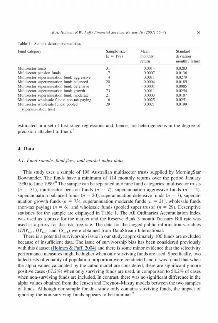
This study uses a sample of 198 Australian multisector trusts supplied by MorningStarDownunder. The funds have a minimum of 114 monthly returns over the period January1990 to June 1999.8 The sample can be separated into nine fund categories: multisector trusts(n � 31), multisector pension funds (n � 7), superannuation aggressive funds (n � 4),superannuation balanced funds (n � 20), superannuation defensive funds (n � 7), superan-nuation growth funds (n � 73), superannuation moderate funds (n � 21), wholesale funds(non-tax paying) (n � 6), and wholesale funds (pooled super trusts) (n � 29). Descriptivestatistics for the sample are displayed in Table 1. The All Ordinaries Accumulation Indexwas used as a proxy for the market and the Reserve Bank 3-month Treasury Bill rate wasused as a proxy for the risk-free rate. The data for the lagged public information variables(TBYt–1, DYt–1, and TSt–1) were obtained from DataStream International.

There is a potential survivorship issue in our study: approximately 100 funds are excludedbecause of insufficient data. The issue of survivorship bias has been considered previouslywith this dataset (Holmes & Faff, 2004) and there is some minor evidence that the selectivityperformance measures might be higher when only surviving funds are used. Specifically, twotailed tests of equality of population proportion were conducted and it was found that whenthe alpha values calculated by the cubic model are considered, there are significantly morepositive cases (67.2%) when only surviving funds are used, in comparison to 58.2% of caseswhen non-surviving funds are included. In contrast, there was no significant difference in thealpha values obtained from the Jensen and Treynor–Mazuy models between the two samplesof funds. Although our sample for this study only contains surviving funds, the impact ofignoring the non-surviving funds appears to be minimal.9

Table 1 Sample descriptive statistics

Fund category Sample size(n � 198)

Meanmonthlyreturn

Standarddeviationmonthly return

Multisector trusts 31 0.0014 0.0283Multisector pension funds 7 0.0007 0.0136Multisector superannuation fund: aggressive 4 0.0011 0.0279Multisector superannuation fund: balanced 20 0.0004 0.0189Multisector superannuation fund: defensive 7 �0.0001 0.0085Multisector superannuation fund: growth 73 0.0011 0.0254Multisector superannuation fund: moderate 21 0.0003 0.0107Multisector wholesale funds: non-tax paying 6 0.0025 0.0251Multisector wholesale funds: pooled

superannuation trust29 0.0021 0.0199

61K.A. Holmes, R.W. Faff / Financial Services Review 16 (2007) 55–71

4.2. Style analysis indices

Meaningful style analysis relies heavily on the choice of style indices. Sharpe (1992)specifies that the set of indices should be as exhaustive as possible, mutually exclusive andthat their returns should differ. In addressing these issues, we choose the following sixindices: (1) Australian Equity (AEQ): Australian DataStream (DS) Market Index; (2) Aus-tralian Fixed Interest (AFI): UBS Composite All Maturities Index; (3) International Equity(IEQ): MSCI World Ex Australian Index; (4) Listed Property (LP): ASX Property TrustIndex; (5) Overseas Fixed Interest (OFI): WD Citigroup G7 All Maturities Index; and (6)Cash: Reserve Bank of Australia 90 day BAB Index.10

5. Results

5.1. Style drift

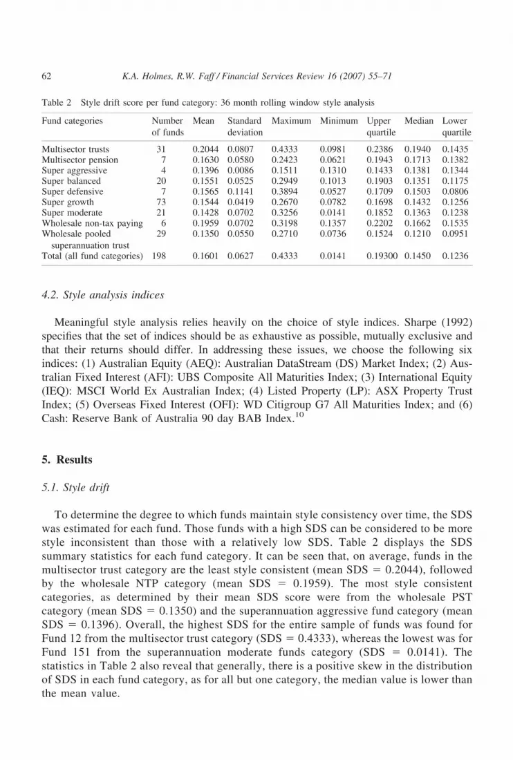
To determine the degree to which funds maintain style consistency over time, the SDSwas estimated for each fund. Those funds with a high SDS can be considered to be morestyle inconsistent than those with a relatively low SDS. Table 2 displays the SDSsummary statistics for each fund category. It can be seen that, on average, funds in themultisector trust category are the least style consistent (mean SDS � 0.2044), followedby the wholesale NTP category (mean SDS � 0.1959). The most style consistentcategories, as determined by their mean SDS score were from the wholesale PSTcategory (mean SDS � 0.1350) and the superannuation aggressive fund category (meanSDS � 0.1396). Overall, the highest SDS for the entire sample of funds was found forFund 12 from the multisector trust category (SDS � 0.4333), whereas the lowest was forFund 151 from the superannuation moderate funds category (SDS � 0.0141). Thestatistics in Table 2 also reveal that generally, there is a positive skew in the distributionof SDS in each fund category, as for all but one category, the median value is lower thanthe mean value.

Table 2 Style drift score per fund category: 36 month rolling window style analysis

Fund categories Numberof funds

Mean Standarddeviation

Maximum Minimum Upperquartile

Median Lowerquartile

Multisector trusts 31 0.2044 0.0807 0.4333 0.0981 0.2386 0.1940 0.1435Multisector pension 7 0.1630 0.0580 0.2423 0.0621 0.1943 0.1713 0.1382Super aggressive 4 0.1396 0.0086 0.1511 0.1310 0.1433 0.1381 0.1344Super balanced 20 0.1551 0.0525 0.2949 0.1013 0.1903 0.1351 0.1175Super defensive 7 0.1565 0.1141 0.3894 0.0527 0.1709 0.1503 0.0806Super growth 73 0.1544 0.0419 0.2670 0.0782 0.1698 0.1432 0.1256Super moderate 21 0.1428 0.0702 0.3256 0.0141 0.1852 0.1363 0.1238Wholesale non-tax paying 6 0.1959 0.0702 0.3198 0.1357 0.2202 0.1662 0.1535Wholesale pooled

superannuation trust29 0.1350 0.0550 0.2710 0.0736 0.1524 0.1210 0.0951

Total (all fund categories) 198 0.1601 0.0627 0.4333 0.0141 0.19300 0.1450 0.1236

62 K.A. Holmes, R.W. Faff / Financial Services Review 16 (2007) 55–71

The SDS is a measure of style consistency derived from the variability of the styleweightings determined through application of a rolling window style analysis process. Thestyle analysis optimization regression aims to maximize the ‘goodness of fit’ of the model,so that fund return can be expressed as a linear combination of the style indices. The degreeto which the linear model can explain the excess fund return is given by the associated R2

value for each fund. Fig. 1 displays the relationship of the R2 value to the associated SDS foreach fund. There is a significant negative correlation between the two measures (�0.2151,p � 0.002), indicating that the amount of variation within the style weightings tends toincrease as the ‘goodness of fit’ of the model decreases.

Following Brown and Harlow’s (2004) line of reasoning, it could be that funds witha low R2 value are basically operating ‘outside of the square’. In other words, their returnseries cannot be explained by the linear combination of six style indices. If this is thecase, then it follows that they may have a higher degree of style inconsistency, as themanager charts his/her own course. However, the case could also be made that the choiceof passive benchmarks used in the style analysis process were not representative of thefund’s actual style and, therefore, the associated low R2 value was more indicative ofineffectual modeling rather than manager skill. Again, this could result in a higherdegree of style inconsistency, because of the difficulty in estimating meaningful styleweights. For this study, the style indices were carefully chosen to avoid significantcollinearity that has been found to reduce the effectiveness of style analysis (Agudo &Gimeno, 2005).

To provide a visual representation and appreciation of style consistency and inconsistency,the style weightings for three funds from each of two main fund categories are displayed in

Fig. 1. Relationship between style drift score and mean R2 values for 36 month rolling window analysis.

63K.A. Holmes, R.W. Faff / Financial Services Review 16 (2007) 55–71

Fig. 2. In each panel, the first fund shown has an SDS very close to the mean SDS for thatcategory, the second fund has the highest SDS for that category, whereas the third fund hasthe lowest SDS for funds in that category. Funds from the multisector trust category aredisplayed in Panel A. Fund 23 has an SDS of 0.2042, which is just below the mean SDS(0.2044) for all multisector trusts in the sample. It can be seen that although the weightingfor the AFI style index is substantial at the start of the sample period, there is a gradualdecrease in this style, and it is replaced primarily by the CASH index towards the end of thesample period. The second fund (#12) displayed in Panel A is the multisector trust fund withthe highest SDS. It is apparent that the gradual change that occurred in the first fund is notevident for Fund 12 and that the changes in the style weightings are far more volatile. Incontrast, the third fund in Panel A, Fund 24, has the lowest SDS of 0.0981. Relative to bothFunds 23 and 12, the changes in the style weightings over time are stable, and a high degreeof style consistency is observed.

The largest fund category (superannuation growth) is represented in Panel B. For thiscategory the mean SDS (0.1544) is similar to that of the balanced super funds, although Fund

Fig. 2. Change in style weights over time for illustrative multisector funds. Panel A, multisector trusts; Panel B:superannuation growth funds.

64 K.A. Holmes, R.W. Faff / Financial Services Review 16 (2007) 55–71

70 with the highest SDS (0.2670) is more style consistent than its counterpart in the balancedfund grouping. Similarly, the super growth fund with the lowest SDS (Fund 128; SDS �0.0782) is more style consistent than the corresponding super balanced fund.

5.2. Cross-sectional analysis

5.2.1. Style drift score and performanceThere is evidence that style consistent funds perform better than funds that demonstrate

inconsistent style (Brown & Harlow, 2004). In this study, we use the SDS as a measure ofthe variability of fund style over time. In Table 3, the correlation coefficients between theSDS for each fund and various fund selectivity performance measures are presented. Thereis considerable variation in the correlation coefficients depending on the performance modelused. The only significant correlation occurs when alpha is obtained from the Treynor–Mazuy market model with conditional variables included. In this case a positive correlation(r � 0.170, p � 0.016) is found, indicating that superior selectivity is related to greater levelsof style drift.

The regression coefficients presented in Table 4 more formally reveal the impact of thedegree of style variability (as measured by the SDS) on fund selectivity measures. Generally,we find that the SDS tends to be positively related to selectivity skill, except in the case of

Table 3 Correlations between cross-sectional variables

Jensenalpha

TMalpha

CondTMalpha

TMKalmanalpha

CondTMKalmanalpha

Cubicalpha

Fundsize

Flowvolatility

MER

TM 0.833(0.000)

1.000

ConditionalTM alpha

0.210(0.003)

0.413(0.000)

1.000

TM Kalmanalpha

0.906(0.000)

0.853(0.000)

0.215(0.000)

1.000

ConditionalTM Kalmanalpha

0.925(0.000)

0.838(0.000)

0.279(0.000)

0.895(0.000)

1.000

Cubic alpha 0.499(0.000)

0.433(0.000)

0.505(0.000)

0.460(0.000)

0.440(0.000)

1.000

Fund size 0.246(0.001)

0.355(0.000)

0.353(0.000)

0.377(0.000)

0.327(0.000)

0.379(0.000)

1.000

Flow volatility �0.009(0.906)

0.012(0.879)

0.023(0.759)

0.008(0.920)

�0.015(0.843)

0.020(0.791)

�0.081(0.280)

1.000

Managementexpenseratios

�0.250(0.012)

�0.161(0.109)

�0.227(0.023)

�0.335(0.001)

�0.298(0.003)

�0.183(0.068)

�0.368(0.000)

0.156(0.122)

1.000

Style driftscore

�0.025(0.731)

0.109(0.128)

0.170(0.016)

�0.042(0.555)

0.031(0.666)

0.020(0.780)

�0.130(0.078)

0.007(0.929)

0.128(0.204)

Note: Pearson correlation coefficient is displayed with p-value in parentheses below. Significant correlations (atthe 5% level) are bolded.

65K.A. Holmes, R.W. Faff / Financial Services Review 16 (2007) 55–71

the Jensen model. In particular, when the alpha derived from the Kalman Filter unconditionalTreynor–Mazuy model is used as the dependent variable, there is a significant (5% level)positive coefficient found (0.0049).

Overall, we find evidence that style drift is related to selectivity skill, although thisconclusion is dependent on the fund performance model. There is some support of a positive

Table 4 Cross-sectional regression results investigating the potential determinants of alpha performance ofAustralian multi-sector managed funds

Dependent variable: alpha coefficients

Independentvariables

UnconditionalJensen model

UnconditionalTreynor-Mazuy model

ConditionalTreynor-mazuymodel

UnconditionalTreynor-MazuyKalman filtermodel

ConditionalTreynor-MazuyKalmanfilter model

Cubicmarketmodel

Multisector trusts 0.0014(1.89)

0.0012(1.22)

0.0016(1.79)

0.012(1.51)

0.0025(3.14)

0.0014(1.43)

Multisector pens 0.0001(0.097)

�0.0002(�0.17)

0.0004(0.40)

0.0003(0.42)

0.0010(1.25)

�0.0001(�0.13)

Super-balanced 0.0009(1.30)

0.0008(0.86)

0.0012(1.41)

0.0007(0.94)

0.0013(1.79)

0.0097(1.08)

Super-defensive �0.0004(�0.64)

�0.0006(�0.84)

�0.0002(�0.30)

0.0003(0.41)

0.0006(0.94)

�0.0006(�0.80)

Super-growth 0.0009(1.46)

0.0007(0.86)

0.0010(1.28)

0.0003(0.42)

0.0009(1.43)

0.0010(1.14)

Super-moderate 0.0002(0.38)

�0.0003(�0.34)

0.0003(0.40)

0.0002(0.27)

0.0011(1.46)

�0.0004(�0.052)

Wholesale non-tax paying

0.0020(3.27)

0.0003(0.29)

0.0008(0.90)

0.0008(1.01)

0.0013(1.65)

0.0005(0.59)

Wholesale pooledsuperannuationtrust

0.0010(2.10)

0.0001(0.16)

0.0005(0.91)

0.0002(0.33)

0.0007(1.27)

0.0004(0.55)

Style drift score �0.0022(�1.22)

0.0011(0.46)

0.0003(0.12)

0.0049(2.59)

0.0027(1.14)

0.0013(0.52)

Size 0.0000(0.23)

0.0002(3.30)

0.0002(3.13)

0.0001(2.22)

0.0001(2.63)

0.0002(2.91)

Flow volatility 0.0004(0.28)

0.0024(1.20)

0.0018(0.92)

�0.0002(�0.094)

0.0006(0.27)

0.0016(0.76)

Managementexpense ratios

�0.0005(�1.66)

�0.0006(�1.54)

�0.0008(�2.1975)

�0.0010(�3.13)

�0.0012(�3.58)

�0.0006(�1.52)

R2 0.611 0.366 0.425 0.530 0.492 0.399

Note: yi � a1D1� a2D2� �3D3� a4D4� a5D5� �6D6� a7D7� a8D8� a10SDSi� a11SIZEi � a12FLOWVOLi

� a13MERi � error, where: D1 � 1 for a multi-sector trust and 0 otherwise; D2 � 1 for a multi-sector pensionand 0 otherwise; D3 � 1 for a balanced super fund and 0 otherwise; D4 � 1 for a defensive super fund and 0otherwise; D5 � 1 for a growth super fund and 0 otherwise; D6 � 1 for a moderate super fund and 0 otherwise;D7 � 1 for a wholesale non-tax paying fund and 0 otherwise; D8 � 1 for a Wholesale PST fund and 0 otherwise;SDSi � style drift score; SIZEi � Fund size (equal to the natural log of mean funds under management for thesample period); FLOWVOLi � Flow Volatility (equal to the variance of the flow during the sample period);MERi � Management Expense Ratio (equal to the median expense ratio for the sample period). The t-statistic isrecorded in parentheses under the estimated coefficient (coefficients significant at the 5% level are bolded).

66 K.A. Holmes, R.W. Faff / Financial Services Review 16 (2007) 55–71

relationship between alpha values and style drift, but the evidence is not consistent across allperformance models.

5.2.2. Flow volatility and fund performanceThere is evidence in the literature of a relationship between fund performance and the

degree of variability in fund flow (Edelen, 1999; Rakowski, 2003; Shoven et al., 2000).To assess this link in our sample, we initially look at the correlation between flowvolatility and various measures of fund selectivity performance (Table 3) and find noevidence of a statistically significant correlation. Regardless of the performance modelused, we find no significant correlation coefficients between any measure of alpha valuesand flow volatility, as measured by the variance of the fund flow. This result is confirmedin Table 4, which contains the cross-sectional regression results, where flow volatility isone of the independent variables and various measures of fund selectivity skill are usedas dependent variables. In Table 4, it can be seen that the regression coefficient for flowvolatility is generally positive (except for the alpha value from the Kalman Filterspecification for the Treynor–Mazuy model; �0.000183), but not significant at the 5%level.

5.2.3. Control variables and performanceThe literature pertaining to the association between fund size and performance finds either

no relationship or an inverse relation (Chan et al., 2002; Chen, Hong, Huang & Kubik, 2004;Gallagher & Martin, 2005; Sawicki & Finn, 2002). Generally, larger funds are not associatedwith superior performance. The correlation coefficients between fund size and all perfor-mance variables used in the present study are presented in Table 3. Interestingly, regardlessof the performance model used, we find a significant positive correlation between fund sizeand all alpha coefficients. When fund size is used as an independent variable againstmeasures of selectivity (Table 4), we find that there is a significant positive relationship,except in the case of the Jensen model.

The literature documents an inverse relationship between MER and fund size (Dowen& Mann, 2004; Geranio & Zanotti, 2005); therefore, we have included MER as across-sectional variable in the present study, and we find similar evidence. In particular,we report a significant negative correlation (r � �0.368, p � 0.000) between fund sizeand MER, suggesting that for funds in our sample there are economies of scaleassociated with the fee structure of larger funds. With regard to fund performance, wefind that MER is significantly negatively correlated with alpha values from three of theperformance models used (correlations vary from �0.335, p � 0.001 to �0.227, p �0.023), implying that higher expense ratios do not lead to associated superior selectionskills (see Table 3). This result is repeated in the cross-sectional regression results shownin Table 4. Specifically, the estimated MER coefficient is consistently negative, and isstatistically significant when alpha is derived from the conditional Treynor–Mazuymodel and the conditional and unconditional versions of the Kalman filter Treynor–Mazuy model.

67K.A. Holmes, R.W. Faff / Financial Services Review 16 (2007) 55–71

6. Conclusions

Using a sample of Australian multisector managed funds, our primary goal was toinvestigate the complex links between style drift, fund flow, and alpha performance. Toevaluate the degree of style drift over the sample period, we use Sharpe’s (1992) styletechnique in the form of a rolling window analysis to produce a series of style weights foreach fund. The variance of these style weights can be interpreted in the form of an SDS,which provides a single quantitative measure of style drift over the sample period (Idzorek& Bertsch, 2004). We provide graphical evidence that the SDS is a meaningful measure ofstyle consistency using our data, and we use the SDS as a key cross-sectional variable alongwith flow volatility (controlling for fund category, fund size and management expense ratio)to determine their influence over fund performance measures.

We find some evidence that SDS is related to fund performance. In particular, whenconditional performance models are used, we find that style drift and selectivity skill arepositively related, indicating that managers that are more successful at stock selection tendto be less consistent with respect to style. With regard to fund flow, we find that it is unrelatedto fund size, style drift, and performance. In secondary findings, we observe that fund sizeis related to fund performance as all alpha values (except for the Jensen model) are positivelyinfluenced by size. In addition, fund size is found to be negatively related to managementexpense ratios, which, in turn, are negatively related to alpha values.

This paper has highlighted the tenuous links between fund flow, style drift, and fundperformance. We have found evidence that successful stock pickers tend to be more variablein style, but that this variability is unrelated to fund flow volatility. Cooper et al. (2005) findthat ‘cosmetic’ style changes, in the form of a name change, can induce substantial fundinflows. In contrast, we find no relationship between the degree of style variability and flowvolatility. However, like us, they find that the fund inflows are unrelated to fund perfor-mance.

From an individual investor’s perspective, this research has several implications. First,many funds appear to suffer from at least moderate cases of style drift and investors shouldtherefore, assess (or gain professional advice on) the extent to which this phenomenon mightbe exposing them to risks with which they would not normally be comfortable. The challengeof doing this in a reliable fashion means that the onus will increasingly fall on the shouldersof professionals. As such, financial planners and investment advisers need to becomeincreasingly aware of the possibility of style drift in funds and seek out mechanisms bywhich they can monitor style changes and trends.

Second, investors need to look below the surface when investing in a particular fund.Although funds with variable style can suggest managers’ inability to maintain a stable styleprofile over time, style drift can also be indicative of superior selectivity skills. Again,financial advisers will need to play a key role in helping to make reliable assessments of thisfor their clients. Third, there might be little to gain by ‘following the pack’ when choosinginvestment vehicles, as we find no evidence that fund flow is related to abnormal fundperformance. That said, investors and advisers will be wise not to become overly confidentabout their abilities to do better than ‘the pack,’ particularly, as is likely, they acknowledgethat their information and skill sets are not superior to many others in the market.

68 K.A. Holmes, R.W. Faff / Financial Services Review 16 (2007) 55–71

Notes

1. Similar to the United States, a significant change in style of Australian funds willbecome apparent to investors ex post when the fund issues an amended prospectus.In Australia, new prospectus’s tend to be issued every six months or so. We thankan anonymous referee for raising our awareness of this issue.

2. The Reserve Bank of Australia Bulletin, February 2003, cites statistics based inFebruary 2001 showing that half of the Australian equities funds offered suchperformance based fees.

3. Similar analysis was also conducted on timing measures of performance, but no clearfindings emerged. Accordingly, these results are suppressed to conserve space; theyare available upon request from the authors.

4. A superannuation fund is an unlisted investment vehicle where investor’s contribu-tions and earnings are redeemed (in total or as a pension) at retirement from theworkforce. Australian superannuation funds are, broadly speaking, equivalent to401(k) plans in the United States. The ‘super’ industry in Australia has experiencedsustained growth for many years because of a range of government policy initiativesover the past two decades. Indeed, superannuation dominates the domestic managedfunds sector.

5. Wholesale funds in Australia target professional investors and are typified by havingquite large minimum investment thresholds. Moreover, wholesale fund transactionstend to be of lower frequency and thus fees charged are lower than ‘retail’ funds. Incontrast, Australian retail funds are targeted at ‘less sophisticated’ investors whowish to transact much more frequently and at lower values (see Morningstar, 2005,p. 11).

6. PST funds pay tax at the fund level. For NTP funds, the tax is paid in the hands ofthe investor.

7. As a robustness check, OLS was also used. Because these results are qualitatively thesame, they are not reported to conserve space.

8. The index series reflects changes in the value of an investment in a fund over time,and is based on a notional $10,000 investment in the fund. Monthly index values arecalculated by reference to the month-end exit price of the fund, which is net ofmanagement fees and assumes reinvestment of all cash and bonus unit distributions.The index series therefore gives representative returns which an actual investor mayhave achieved and measures the monthly performance of the fund.

9. In any case, the rolling window analysis that we employ is infeasible or pointless forfunds that do not meet the data requirements imposed. This represents one of theimplicit costs in adopting a particular research design, unavoidable when it comes toweighing up all the research design tradeoffs.

10. Initially eleven style indices were considered, but five (ASX Small Ordinaries; ASXSE Russell All Value Index; ASX SE Russell All Value Growth; SandP/ASX 50 DSIndex; SandP/ASX 100 DS Index) were discarded after significant return correlationswere found between the indices and the AEQ index. In addition to the correlations,tests of equality of variances were conducted between the AEQ index and each of the

69K.A. Holmes, R.W. Faff / Financial Services Review 16 (2007) 55–71

five indices and no significant differences in variance were found. On this basis onlythe six indices mentioned above were included in the style analysis process.

Acknowledgments

The authors gratefully acknowledge the helpful comments of Karen Benson and ananonymous referee. We also thank Kylie Moreland for her very careful proofreading skills.

References

Agudo, L. F., & Gimeno, L. A. (2005). Effects of multicollinearity on the definition of mutual funds’ strategicstyle: the Spanish case. Applied Economics Letters, 12, 553–556.

Berk, J., & Green, R. (2004). Mutual fund flows and performance in rational markets. Journal of PoliticalEconomy, 112, 1269–1295.

Black, A., Fraser, P., & Power, D. (1992). UK unit trust performance 1980–1989: a passive time-varyingapproach. Journal of Banking and Finance, 16, 1015–1033.

Brown, K., & Harlow, W. (2004). Staying the course: performance persistence and the role of investment styleconsistency in professional asset management. Available at: http://papers.ssrn.com/sol3/papers.cfm?abstract_id�306999.

Brown, K., Harlow, W., & Starks, L. (1996). Of tournaments and temptations: an analysis of managerialincentives in the mutual fund industry. Journal of Finance, 51, 85–110.

Brown, S. J., & Goetzmann, W. (1997). Mutual fund styles. Journal of Financial Economics, 43, 373–399.Chan, L., Chen, H., & Lakonishok, J. (2002). On mutual fund investment styles. Review of Financial Studies, 15,

1407–1437.Chen, J., Hong, H., Huang, M., & Kubik, J. D. (2004). Does fund size erode mutual fund performance? The role

of liquidity and organization. The American Economic Review, 94, 1276–1302.Chevalier, J., & Ellison, G. (1997). Risk taking by mutual funds as a response to incentives. Journal of Political

Economy, 105, 1167–1200.Cooper, M., Gulen, H., & Rau, P. R. (2005). Changing names with style: mutual fund name changes and their

effects on fund flows. Journal of Finance, 60, 2825–2858.Deaves, R. (2004). Data-conditioning biases, performance, persistence and flows: the case of Canadian Equity

Funds. Journal of Banking and Finance, 28, 673–694.DelGuercio, D., & Tkac, P. (2002). The determinants of the flow of funds of managed portfolios: mutual funds

versus pension funds. Journal of Financial and Quantitative Analysis, 37, 523–558.Dowen, R. J., & Mann, T. (2004). Mutual fund performance, management behaviour, and investor costs.

Financial Services Review, 13, 79–91.Edelen, R. (1999). Investor flows and the assessed performance of open-ended mutual funds. Journal of Financial

Economics, 53, 439–466.Gallagher, D. R., & Martin, K. M. (2005). Size and investment performance: a research note. Abacus, 41, 55–65.Gallo, J. G., & Lockwood, L. J. (1999). Fund management changes and equity style shifts. Financial Analysts

Journal, 55, 44–52.Geranio, M., & Zanotti, G. (2005). Can mutual funds characteristics explain fees? Journal of Multinational

Financial Management, 15, 354–376.Holmes, K. A., & Faff, R. W. (2004). Stability, asymmetry and seasonality of fund performance: an analysis of

Australian multi-sector managed funds. Journal of Business Finance and Accounting, 31, 539–578.Idzorek, T., & Bertsch, F. (2004). The style drift score. Journal of Portfolio Management, 31, 76–84.Jain, P., & Wu, J. (2000). Truth in mutual fund advertising: evidence on future performance and fund flows.

Journal of Finance, 55, 937–958.

70 K.A. Holmes, R.W. Faff / Financial Services Review 16 (2007) 55–71

Jensen, M. (1968). The performance of mutual funds in the period 1945–64. Journal of Finance, 23, 389–416.Kim, M., Shukla, R., & Thomas, M. (2000). Mutual fund objective misclassification. Journal of Economics and

Business, 52, 309–323.Moringstar. (2005). Classification policy. Australian investments. Available at: http://www.morningstar.

com.au/productpages/Investment%20classification_policy.pdf#search�%22australian%20wholesale%20funds%20definition%22. Accessed August 19, 2006.

Rakowski, D. (2003). Fund flow volatility and performance. Georgia State University, Working paper.Reserve Bank of Australia. (2003). Australian funds management: market structure and fees. RBA Bulletin,

February, 55–62.Sawicki, J., & Finn, F. (2002). Smart money and small funds. Journal of Business Finance and Accounting, 29,

825–846.Sawicki, J., & Ong, F. (2000). Evaluating managed fund performance using conditional measures: Australian

evidence. Pacific-Basin Finance Journal, 8, 505–528.Sharpe, W. F. (1992). Asset allocation: management style and performance measurement. Journal of Portfolio

Management, 18, 7–19.Shoven, J., Dickson, J., & Sialm, C. (2000). Tax externalities of equity mutual funds. NBER Working Paper,

W7669.Sirri, E., & Tufano, P. (1998). Costly search and mutual fund flows. Journal of Finance, 53, 1589–1622.Swinkels, L., & Van Der Sluis, P. J. (2001). Return-based style analysis with time-varying exposures. Available

at: http://greywww.kub.nl:2080/greyfiles/center/2001/doc/96.pdf.Treynor, J., & Mazuy, K. (1966). Can mutual funds outguess the market? Harvard Business Review, 44, 131–136.Zeckhauser, R., Patel, J., & Hendricks, D. (1991). Nonrational actors and financial market behaviour. Theory and

Decision, 1, 257–287.

71K.A. Holmes, R.W. Faff / Financial Services Review 16 (2007) 55–71