Lidar sounding of volcanic plumes

Luca Fiorani*a, Alessandro Aiuppab, Federico Angelinia, Rodolfo Borellia, Mario Del Francoc, Daniele Murrad, Marco Pistillia, Adriana Puiua, Simone Santorob

aDiagnostics and Metrology Laboratory, Italian National Agency for New Technologies, Energy and Sustainable Economic Development, Via Enrico Fermi 45, 00044 Frascati, Italy; bEarth and Sea

Sciences Department, University of Palermo, Via Archirafi 36, 90123 Palermo, Italy; cMathematical Modeling Laboratory, Italian National Agency for New Technologies, Energy and Sustainable

Economic Development, Via Enrico Fermi 45, 00044 Frascati, Italy; dRadiation Sources Laboratory, Italian National Agency for New Technologies, Energy and Sustainable Economic Development,

Via Enrico Fermi 45, 00044 Frascati, Italy

ABSTRACT

Accurate knowledge of gas composition in volcanic plumes has high scientific and societal value. On the one hand, it gives information on the geophysical processes taking place inside volcanos; on the other hand, it provides alert on possible eruptions. For this reasons, it has been suggested to monitor volcanic plumes by lidar. In particular, one of the aims of the FP7 ERC project BRIDGE is the measurement of CO2 concentration in volcanic gases by differential absorption lidar. This is a very challenging task due to the harsh environment, the narrowness and weakness of the CO2 absorption lines and the difficulty to procure a suitable laser source. This paper, after a review on remote sensing of volcanic plumes, reports on the current progress of the lidar system.

Keywords: lidar, differential absorption, aerosol load, water vapor, carbon dioxide, volcanic plumes

1. INTRODUCTION The composition of volcanic gases gives information on the processes inside volcanos and on the transition from quiescence to eruption. Up to now, coupled gas-geophysical studies are sparse, due to the difference in their typical sampling frequency (> 1 Hz for seismic signals and < 10-5 Hz for gas data). This explains the interest of geophysicists in new techniques of gas detection, in particular for CO2, the second most abundant gas in volcanic fluids and the most directly linked to deep “pre-eruptive” volcanic degassing processes.

Lidars1 have been used in the past to determine aerosol load2, SO2 concentration3 and water vapor flux in volcanic plumes4. One of the tasks of the recently begun FP7 ERC project BRIDGE5 is the lidar measurement of CO2 concentration in volcanic plumes.

A lidar is composed of a transmitter (laser) and a receiver (telescope). Its principle of operation is illustrated in Figure 1a: the backscatterers (molecules and aerosols) at the distance R from the system send back part of the laser pulse toward A, active surface of the telescope. Consequently, the analysis of the detected signal as a function of t, time interval between emission and detection, allows one to study the optical properties of the atmosphere along the beam, since the simple relation between t and R is given by:

2ctR = (1)

where c is the speed of light.

*luca.fiorani@enea.it; phone 39 06 9400-5861; fax 39 06 9400-5312; www.enea.it

Lidar Technologies, Techniques, and Measurements for Atmospheric Remote Sensing IX, edited by Upendra N. Singh, Gelsomina Pappalardo, Proc. of SPIE Vol. 8894, 889407

© 2013 SPIE · CCC code: 0277-786X/13/$18 · doi: 10.1117/12.2028364

Proc. of SPIE Vol. 8894 889407-1

Downloaded From: http://proceedings.spiedigitallibrary.org/ on 12/07/2013 Terms of Use: http://spiedl.org/terms

2.5E 04

`E 2.0E-04cw

1.5E-04

3=

c 1.0E-04o

5.0E-05w

0.0E+00

0 1000 2000 3000

Altitude [m]

4000 5000

The photons detected within τD, detector response time, are backscattered from the layer delimited by the distances R and R+cτD/2. Their number n is proportional to the thickness cτD/2 and to the backscattering coefficient β of the involved air volume. Furthermore, in its round trip, the original pulse consisting of n0 photons is attenuated by the atmosphere. This phenomenon is quantified by the extinction coefficient α. Moreover, n is proportional to the solid angle A/R2 and the efficiency ζ of the detection system.

a

A ζ

α β

R τc D2

n0

b Figure 1. a) Lidar principle of operation. The points represent generic atmospheric scatterers (molecules and aerosols). b) Extinction coefficient retrieved from the lidar signal. The double peak from 1800 to 3300 m appears to superimpose over a nearly linear decay and are due to the volcanic plume (the dashed line has been added for the convenience of the reader).

On the basis of the preceding discussion, the elastic lidar equation can be written:

( ) ( ) ( ) ( ) ( ) ⎥⎦

⎤⎢⎣

⎡′′−= ∫

RD RdRcR

RAnRn

020 ,2exp

2,, λατλβλζλλ . (2)

The coefficients α and β are linked one to another and are proportional to the aerosol load. An example of elastic lidar application to a volcanic plume is given in Figure 1b (Mount Etna, Italy, 14 July 2008)2.

Laser remote sensing can also be used to measure the concentration of water vapor and atmospheric gases by DIAL1. This system is based on the detection of backscattered photons from laser pulses transmitted to the atmosphere at two different wavelengths. At one wavelength (λOFF), the light is almost only scattered by air molecules and aerosols, whereas at the other one (λON), it is also absorbed by the gas under study. The difference between the two recorded signals is thus related to the pollutant concentration. More precisely, on the basis of equation (2), if λOFF and λON are close enough, as in the case of water vapor, SO2 and CO2 measurement, the simplified DIAL equation can be derived:

( ) ( ) ( )[ ]( )( ) ⎥⎦

⎤⎢⎣

⎡−

=ON

OFF

OFFON RnRn

dRdRC

λλ

λσλσ ,,ln

21

. (3)

where C(R) and σ(λ) are, respectively, the concentration and the absorption cross-section of the gas molecule.

The DIAL principle of operation is illustrated in Figure 2a. An example of DIAL application to a volcanic plume is given in Figure 2b (Stromboli Volcano, Italy, 17 September 2009)4.

The lidar under development for the BRIDGE project will be positioned below the volcanic plume that will be probed with the laser beam. With such configuration, and scanning the plume in a vertical plane roughly perpendicular to the plume axis, the CO2 concentrations outside and inside the volcanic plume will be measured. In practice, the lidar will be aimed directing its optical axis by means of plain mirrors. These measurements, once integrated over the whole cross-sectional area of the plume, and upon scaling to the plume transport rate (as derived from the wind speed at the plume altitude), will allow the retrieval of the CO2 flux.

As we have seen, the lidar return is linked to the optical properties of the atmosphere along the laser beam. In general, the extinction and backscattering coefficient are determined mainly by the aerosols load. This means that the lidar will not only measure gas concentrations but also aerosol loads.

The system could also be used for the measurement of wind speed4, thanks to the ability of steering the optics in different directions. According to equation (2), the number of photons backscattered by the atmosphere at a given distance from

Proc. of SPIE Vol. 8894 889407-2

Downloaded From: http://proceedings.spiedigitallibrary.org/ on 12/07/2013 Terms of Use: http://spiedl.org/terms

OFF

ON

P

pOFF

PON

Ro

pOFF

PON

0

1 d DOFFC = ln

?46 dR pON

o

R

R

200 700Distance [m]

C [torr]36

30

24

18

12

6

o

the instrument is proportional to the backscattering coefficient. This factor is a function of the density of aerosols responsible for the light scattering. Any change in its spatio-temporal distribution during a data acquisition will lead therefore to variations in the lidar returns from one laser shot to another. In particular, a wind flow along the beam axis will be detected from the transport of the spatial inhomogeneities of β along the optical path.

a b Figure 2. a) DIAL principle of operation. The figure does not represent the actual geometry of the experiment. b) Water vapor concentration retrieved by DIAL. The white points are the lidar measurements. The black cross is the point where the concentration maximum of the scan occurred.

2. LASER CHOICE CO2 absorbs in the 15, 4.2, 2.1 and 1.6 µm bands (in order of decreasing strength)6. Unfortunately, in the first two bands viable lasers are not available and atmospheric backscattering is rather low, so the 2.1 and 1.6 µm bands have been suggested for its detection7. Nevertheless, the DIAL measurement of CO2 remains a difficult task because the absorption lines are narrow and weak8.

For all these reasons, a powerful, tunable and narrow-linewidth laser source is highly desirable. Laser technology is a rapidly evolving field. Dye lasers of new conception and OPOs (optical parametric oscillators) are now available as tunable sources in spectroscopic researches thanks to the relevant advantage of narrow linewidth. Nevertheless, up to now, all these sources have been mainly employed in the laboratory because of their relative complexity and fragility. Recently, some narrow-linewidth sources characterized by computer controlled alignment and sealed housing have been developed, making thus possible their deployment in field measurement campaigns. Fiber lasers are also a possible choice. They are more robust and small but have a very limited tunability: the lidar transmitter could contain two of them, the first one tuned at λOFF and the second one tuned at λON.

Recently, Tm,Ho:YLF lasers lasers have been employed for DIAL measurements of atmospheric CO2 for climatic studies9, 10. Although these sources are attractive for their high energy and narrow linewidth, they have two major drawbacks: their range of tunability is very narrow (few tenths of nm) if compared with that of dye lasers and OPOs (about 1 μm), thus allowing the measurement of only carbon dioxide (and not necessarily with the best line that could be out of the tunability interval)11; they are very complex system, not ready for the market and hardly suitable to field applications.

Thanks to their wide range of tunability from UV (ultraviolet) to near IR (infrared) and the occurrence of many absorption lines in these spectroscopic regions, dye lasers and OPOs will make possible to measure not only CO2, but many other species relevant to volcanic phenomena and atmospheric chemistry.

Proc. of SPIE Vol. 8894 889407-3

Downloaded From: http://proceedings.spiedigitallibrary.org/ on 12/07/2013 Terms of Use: http://spiedl.org/terms

1064 nm delay

532 nm

Oscillator Pre -Amp Main Amp(EBP)

IK

output

PrecisionScan Dye Laser telescope

1 1dichroic DFM dichroicmirror LiNb03 mirror

OPALiNb03

Ul 1/J4[11 1,1 VLL11

dump

OPANIR

reversing beamsplitter prism

runitersingve

pump beambeam Splitter t, I

cylindrical A internal SHG oetion

ensesoutput

grating

coupler beam expansion

n

pyroelectricsplit detector

doubling compensator Pellin -Broca

Hcrystal posma .

\\Mri yiè./.beamreversion 20 mm dye cell I W telescope 140 remrnm dye cell

1

W

Another advantage of dye lasers and OPOs is that they are pumped by Nd:YAG lasers. A frequency tripled Nd:YAG laser has already been employed for Raman lidar measurement of CO2 in the atmosphere12, thus giving another string to our bow, although the absolute calibration of Raman lidar remains a difficult task.

After a long and accurate research at the world’s leading manufacturers, the laser system shown in Figure 3 has been purchased from Sirah. Its main characteristic is that the beam at 634 or 703 nm emitted by the dye laser is used to generate 1570 and 2070 nm, respectively, by difference frequency mixing with the Nd:YAG fundamental.

a

b Figure 3. a) Laser system manufactured by Sirah. SHG: second harmonic generator, EBP: enhanced beam profile cell, DFM: difference frequency mixing, OPA: optical parametric oscillator. b) Detailed scheme of the dye laser and of the optional SHG.

The system has some remarkable features:

1. 10 pm stability corresponding to 0.25 and 0.2 cm-1 stability at 1570 and 2070 nm, respectively;

2. dynamic mode option;

3. piezo wavelength control;

4. Visible and UV emission, this latter with the second harmonic generation (optional).

The longitudinal mode spacing of the dye laser resonator is 0.018 cm-1. Its linewidth is 1.2 pm which corresponds to 0.03 and 0.025 cm-1 at 634 and 703 nm, respectively. This means that two longitudinal modes will be emitted. Unfortunately, the mode structure is not predictable nor constant over minutes: this means that during a lidar experiment energy could distributed in unknown and unequal parts in the two modes, causing a serious problem due to the narrow bandwidth of the CO2 absorption lines. In order to overcome this difficulty, Sirah developed the dynamic mode option (patent

Proc. of SPIE Vol. 8894 889407-4

Downloaded From: http://proceedings.spiedigitallibrary.org/ on 12/07/2013 Terms of Use: http://spiedl.org/terms

pending): a piezo changes the resonator length of the dye laser between every shot, thus modifying the longitudinal mode structure for successive laser pulses. Hence the spectral shape for successive laser pulses is statistically distributed (in our case 50% of the energy is emitted in each mode) and artifacts due to the longitudinal mode structure are suppressed.

Piezo wavelength control allows just one laser system to fire at λON and after 1/10 of second at λOFF. This is achieved as follows:

• the rotatable Littrow grating is mounted on a tilt piezo (the silver block behind the grating with diagonal slit and black cable shown in Figure 4a; with this tilt piezo the wavelength between successive Nd:YAG laser shots is changed so that one shot is fired at λON and the other one at λOFF;

• although the piezo is fast enough for a 10 Hz repetition rate, the two nonlinear crystals inside the IR unit cannot be moved so fast; therefore two more nonlinear crystals have to be mounted, the first one after the standard mixing crystal and the second one after the standard amplifier crystal; these two new crystals have to be mounted with a slightly different angle in order to produce λOFF: this is achieved by a special mechanics allowing the adjustment of the new crystal to the slightly different angle with a micrometric screw (Figure 4b).

The visible and UV emissions of the system could be used for the spectroscopic measurement of other species (e.g. SO2, another key molecule of volcanic plumes).

a b Figure 4. a) Rotatable Littrow grating. b) Assembly of the double crystal.

3. LIDAR SIMULATION Two lidar system have been considered, according to Table 1.

Table 1. Wavelengths and absorption coefficients8 of two possible lidar systems.

System λON [nm] λOFF [nm] αON [m-1] αOFF [m-1] 1 – Lidar in the 1.6 µm spectral region 1572.6 1572.5 1.1×10-1 9.0×10-3 2 – Lidar in the 2.1 µm spectral region 2011.5 2011.9 6.0 3.5×10-1

Laser beam and volcanic plume are orthogonal. This latter extends from 3000 to 3500 m of range. If not stated otherwise, the lidar elevation angle is 10°. Aerosol is simulated according to continental cumulus described by Pruppacher and Klett13 but with a 10 times less numerical concentration. Background CO2 concentration is 391 ppm, while maximum CO2 concentration in the volcanic plume14 is 2×105 ppm. Both aerosol and CO2 profiles are assumed to be Gaussian (Figure 5). Aerosol extinction and backscattering coefficients are retrieved at the selected wavelengths by Mie calculations. Extinction coefficients for molecules, aerosols and CO2 are shown in Figure 6.

The atmospheric transmission changes drastically between 1572 and 2011 nm, being the absorption coefficient of CO2 two orders of magnitude larger at the longer wavelength. At 1572 nm the aerosol extinction is comparable to that of CO2 inside the plume, while at 2011 nm the CO2 extinction is dominant even in the background zone (outside the plume).

Proc. of SPIE Vol. 8894 889407-5

Downloaded From: http://proceedings.spiedigitallibrary.org/ on 12/07/2013 Terms of Use: http://spiedl.org/terms

14

12

10

pÑ 8U

6

4

2

03000 3050 3100 3150 3200 3250 3300 3350 3400 3450 3500

distance from fidar, m

Extinction coefficient inside the plume @ 2011.5nm

me optical depth: 3.086

Figure 5. a) Gaussian shape of the volcanic plume.

a0 500 1000 1500 2000 2500 3000 3500 4000 4500 5000

10-4

10-3

10-2

10-1

100

101

102

103extinction coefficients, km-1 @ 1572.6 nm - 60° elevation

distance from lidar, m

ext c

oeff,

km

-1

molecularaerosolads-onads-off

b0 500 1000 1500 2000 2500 3000 3500 4000 4500 5000

10-4

10-3

10-2

10-1

100

101

102

103extinction coefficients, km-1 @ 2011.5 nm - 60° elevation

distance from lidar, m

ext c

oeff,

km

-1

molecularaerosolads-onads-off

Figure 6. Extinction coefficients at a) 1572 and b) 2011 nm for molecules, aerosols and CO2 (lidar elevation angle 60°).

a0 500 1000 1500 2000 2500 3000 3500 4000 4500 5000

10-22

10-20

10-18

10-16

10-14

10-12

distance from lidar, m

sign

al, a

.u.

Synthetic DIAL echoes from volcanic plume @ 1572.6 nm - 10° elevation

molecularmol+aerads-onads-off

b500 1000 1500 2000 2500 3000 3500 4000 4500 5000 5500

10-35

10-30

10-25

10-20

10-15

distance from lidar, m

sign

al, a

.u.

Synthetic DIAL echoes from volcanic plume @ 2011.5 nm - 10° elevation

molecularmol+aerads-onads-off

Figure 7. Lidar echoes simulated at a) 1572 and b) 2011 nm (lidar elevation angle 10°).

Proc. of SPIE Vol. 8894 889407-6

Downloaded From: http://proceedings.spiedigitallibrary.org/ on 12/07/2013 Terms of Use: http://spiedl.org/terms

Lidar echoes have been calculated by the lidar equation. Results are shown in Figure 7 for both 1572 and 2011 nm. The signal at 2011 nm is strongly extinguished by CO2, giving an optical depth of the plume of several orders of magnitude. This would require a very sensitive instrument and background noise could be very limiting, although the background has not been taken into account to evaluate the signal-to-noise ratio. This aspect would require accurate calculations of the aerosol cross section, atmospheric radiative transfer and the knowledge of the laser power to couple the signal power to the background light.

The simulated CO2 concentration inside the volcanic plume can be regarded as the maximum possible, i.e. it is expected just outside the crater. At some km from volcanos an excess of only some tens of ppm can be found. A too strong absorption will lead to the extinction of the signal over short ranges, while a more moderate absorption will allow the observation of the plume from further distances. Crossing the plume at slant angles would provide higher sensitivity because of the increased optical path. On the other hand, it is not always possible to choose such angle over a large range, since the geometry of the observation system depends on the geometry of the plume that is determined by a lot of parameters: atmospheric stability conditions, wind-induced dispersion and capping.

For these reasons, a system operational in a wide range of conditions is desirable: according to Table 2 a system able to operate both in the 1.6 and 2.1 µm spectral regions would be able to operate in many real scenarios.

Table 2. Main characteristics of two possible lidar systems.

System Absorption Sensitivity Range Application

1 – Lidar in the 1.6 µm spectral region Moderate Low Long High CO2 concentrations orremote observation

2 – Lidar in the 2.1 µm spectral region Strong High Short Low CO2 concentrations orclose observation

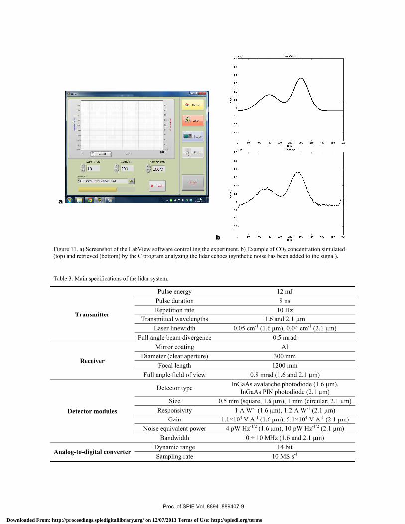
4. CURRENT PROGRESS The procurement of the main components of the lidar system (laser system, telescope, detector modules in the 1.6 and 2.1 µm spectral regions, analog-to-digital converter) has been completed. The laser system is under test in our laboratory and results with a CO2-filled absorption cell confirm the specification provided by Sirah (Figure 8). The ray tracing shows that the detectors, having size of 0.5 mm (1.6 µm) and 1 mm (2.1 µm) will collect all the lidar return, taking into account the beam divergence (Figure 9). The final mechanical frame where the lidar system will be hosted has been designed (Figure 10) and is in advanced stage of realization. The LabView software controlling the experiment and the C program analyzing the lidar echoes are nearly completed (Figure 11). The main specifications of the lidar system are listed in Table 3.

5. CONCLUSIONS The DIAL technique has been briefly reviewed, having in mind its application to the remote measurement of CO2 concentration in volcanic plumes. Unlike measurements for climatic purposes, CO2 concentration in volcanic plumes can vary of some order of magnitudes. Also the measurement geometry, and in particular the distance between system and volcano, depends heavily from the measurement scenario. For these reasons, it has been decided to develop a lidar transmitting both in the 1.6 and 2.1 µm spectral regions. Lidar echoes have been simulated in an extreme case in both spectral regions. Eventually, the current progress of the system has been outlined.

ACKNOWLEDGEMENTS The authors are grateful to R. Fantoni and A. Palucci for constant encouragement. They thank L. Cannilla for procurement assistance, Sirah and Laser Optronic for laser customization (P. Jauernik and S. De Pascalis) and installation (A. Wloka and P. Stropiccioli), Marcon Telescopes (L. Marcon) for telescope elements, LAV Coatings (E. Giannelli) for telescope coatings, Licel (B. Stein) and Hamamatsu (M. Aversa) for custom designed 1.6 and 2.1 µm detectors and Impat (M. Mantovani and S. Mantovani) for mechanical development. The support from the FP7 ERC project BRIDGE, research project contract 305377, is gratefully acknowledged.

Proc. of SPIE Vol. 8894 889407-7

Downloaded From: http://proceedings.spiedigitallibrary.org/ on 12/07/2013 Terms of Use: http://spiedl.org/terms

1.05

1.00

n ati

Transmittance vs Wavenumber (cm-1) - 19/06/2013-HITRAN

Low Resolution

High Resolution

dv...i..'

0.90

0.85

6359.5 6360.0 6360.5 6361.0 6361.5 6362.0

1066 nm Beam Laser

15)tú9 B15ß,39 nm Beam Laser

Detector p)

-1 I

Cell184 an

CO2 Flow (in)

Oz Flow (out)

Windows at Brewsters Angle

Nd:YAG Laser

Precision ScanDye Laser OPANIR

Detector pa)

30cm

update set s Fant window led zoom

LE

CONFIGURATION I OF

a b Figure 8. a) Transmittance measured in a b) CO2-filled absorption cell. Points: experimental measurement. Line: HITRAN data8.

a b Figure 9. a) Ray-tracing of the light collected by the 1.6-µm detector (vertical line) preceded by an optical window and a meniscus lens (full angle field of view: 0.8 mrad). b) Spot diagram of the light collected by the 1.6-µm detector.

Figure 10. Mechanical frame of the lidar system (on the left two steering mirror to aim it to the target).

Proc. of SPIE Vol. 8894 889407-8

Downloaded From: http://proceedings.spiedigitallibrary.org/ on 12/07/2013 Terms of Use: http://spiedl.org/terms

Laser shots

J LO

Samples

vi 200

FC:\USers\USefl\Desktop\runl

Sample Rate

.00M

Save

Home

® Scopé.

Prog

STOP'

1-4 71 477T

CCO2(R)

50 100 150 200 250 300 350 400 450

R (m)

500

50 100 150 200 250 300

R (m)

350 400 450 500

a

bFigure 11. a) Screenshot of the LabView software controlling the experiment. b) Example of CO2 concentration simulated (top) and retrieved (bottom) by the C program analyzing the lidar echoes (synthetic noise has been added to the signal).

Table 3. Main specifications of the lidar system.

Transmitter

Pulse energy 12 mJ Pulse duration 8 ns Repetition rate 10 Hz

Transmitted wavelengths 1.6 and 2.1 µm Laser linewidth 0.05 cm-1 (1.6 µm), 0.04 cm-1 (2.1 µm)

Full angle beam divergence 0.5 mrad

Receiver

Mirror coating Al Diameter (clear aperture) 300 mm

Focal length 1200 mm Full angle field of view 0.8 mrad (1.6 and 2.1 µm)

Detector modules

Detector type InGaAs avalanche photodiode (1.6 µm), InGaAs PIN photodiode (2.1 µm)

Size 0.5 mm (square, 1.6 µm), 1 mm (circular, 2.1 µm) Responsivity 1 A W-1 (1.6 µm), 1.2 A W-1 (2.1 µm)

Gain 1.1×104 V A-1 (1.6 µm), 5.1×104 V A-1 (2.1 µm) Noise equivalent power 4 pW Hz-1/2 (1.6 µm), 10 pW Hz-1/2 (2.1 µm)

Bandwidth 0 ÷ 10 MHz (1.6 and 2.1 µm)

Analog-to-digital converter Dynamic range 14 bit Sampling rate 10 MS s-1

Proc. of SPIE Vol. 8894 889407-9

Downloaded From: http://proceedings.spiedigitallibrary.org/ on 12/07/2013 Terms of Use: http://spiedl.org/terms

REFERENCES

[1] L. Fiorani, “Lidar application to litosphere, hydrosphere and atmosphere,” in Progress in Laser and Electro-Optics Research, V. V. Koslovskiy, ed., 21-75 (Nova, New York, 2010).

[2] L. Fiorani, F. Colao, and A. Palucci, “Measurement of Mount Etna plume by CO2-laser-based lidar,” Opt. Lett. 34, 800-802 (2009).

[3] P. Weibring, H. Edner, S. Svanberg, G. Cecchi, L. Pantani, R. Ferrara, and T. Caltabiano, “Monitoring of volcanic sulphur dioxide emissions using differential absorption lidar (DIAL), differential optical absorption spectroscopy (DOAS), and correlation spectroscopy (COSPEC),” Appl. Phys. B 67, 419–426 (1998).

[4] L. Fiorani, F. Colao, A. Palucci, D. Poreh, A. Aiuppa, and G. Giudice, “First-time lidar measurement of water vapor flux in a volcanic plume,” Opt. Comm. 284, 1295–1298 (2011).

[5] European Research Council, project n. 305377: BRIDGE – Bridging the gap between gas emissions and geophysical observations at active volcanoes.

[6] P. J. Linstrom and W. G. Mallard, “The NIST Chemistry WebBook: A Chemical Data Resource on the Internet”, J. Chem. Eng. Data 46, 1059-1063 (2001).

[7] R. T. Menzies and D. M. Tratt, “Differential laser absorption spectrometry for global profiling of tropospheric carbon dioxide: selection of optimum sounding frequencies for high-precision measurements,” Appl. Opt. 42, 6569-6577 (2003).

[8] L. S. Rothman, I. E. Gordon, A. Barbe, D. C. Benner, P. F. Bernath, M. Birk, V. Boudon, L. R. Brown, A. Campargue, J.-P. Champion, K. Chance, L. H. Coudert, V. Dana, V. M. Devi, S. Fally, J.-M. Flaud, R. R. Gamache, A. Goldman, D. Jacquemart, I. Kleiner, N. Lacome, W. J. Lafferty, J.-Y. Mandin, S. T. Massie, S. N. Mikhailenko, C. E. Miller, N. Moazzen-Ahmadi, O. V. Naumenko, A. V. Nikitin, J. Orphal, V. I. Perevalov, A. Perrin, A. Predoi-Cross, C. P. Rinsland, M. Rotger, M. Šimečková, M. A. H. Smith, K. Sung, S. A. Tashkun, J. Tennyson, R. A. Toth, A. C. Vandaele, and J. VanderAuwera, “The HITRAN 2008 molecular spectroscopic database,” J. Quant. Spectrosc. Radiat. Transfer 110, 533-572 (2009).

[9] F. Gibert, P. H. Flamant, J. Cuesta, and D. Bruneau, “Vertical 2-µm heterodyne differential absorption lidar measurements of mean CO2 mixing ratio in the troposphere,” J. Atm. Ocean. Tech. 25, 1478-1497 (2008).

[10] G. J. Koch, J. Y. Beyon, F. Gibert, B. W. Barnes, S. Ismail. M. Petros, P. J. Petzar, J. Yu, E. A. Modlin, K. J. Davis, and U. N. Singh, “Side-line tunable laser transmitter for differential absorption lidar measurements of CO2: design and application to atmospheric measurements,” Appl. Opt. 47, 944-956 (2008).

[11] L. Fiorani, W. R. Saleh, M. Burton, A. Puiu, and M. Queißer, “Spectroscopic considerations on DIAL measurement of carbon dioxide in volcanic emissions,” J. Optoelectron. Adv. M. 15, 317-325 (2013).

[12] D. N. Whiteman, K. Rush, I. Veselovskii, M. Cadirola, J. Comer, J. R. Potter, and R. Tola, “Demonstration measurements of water vapor, cirrus clouds, and carbon dioxide using a high-performance Raman lidar,” J. Atm. Ocean. Tech. 24, 1377–1388 (2007).

[13] H. R. Pruppacher and J. D. Klett, Microphysics of Clouds and Precipitation (Springer, Dordrecht, 2010). [14] T. Mori and K. Notsu, “Temporal variation in chemical composition of the volcanic plume from Aso volcano,

Japan, measured by remote FT-IR spectroscopy,” Geochem. J. 42, pp. 133–140 (2008).

Proc. of SPIE Vol. 8894 889407-10

Downloaded From: http://proceedings.spiedigitallibrary.org/ on 12/07/2013 Terms of Use: http://spiedl.org/terms