Tax reform results with different demand systems

Journal of Public Economics 41 (1990) 277-296. North-Holland

TAX REFORM RESULTS WITH DIFFERENT DEMAND SYSTEMS

Andre DECOSTER and Erik SCHOKKAERT*

Centrum voor Economische Studien, Katholieke Universiteit Leuven, E. van Evenstraat ZB, B-3000 Leuven, Belgium

Received August 1987, revised version received December 1989

We calculate the marginal welfare costs for a twelve-commodity classification of the Belgian indirect tax system. Price elasticities are estimated with Rotterdam, AIDS, CBS and the linear expenditure system. The ranking of the marginal welfare costs is similar when we use unrestricted estimates of the first three systems. After the symmetry condition of the Slutsky matrix is imposed, the differences become more important. However, they diminish with increasing inequality aversion.

1. Introduction

A major obstacle to the practical application of optimal taxation theory is the dependence of the results on the specification of the demand system used to estimate the reactions of the consumers. [See, for example, Deaton (1981) and, for an empirical illustration, Ray (1986).] There are many reasons, however, to hypothesize that the problem might be less severe in the context of marginal tax reform. This is emphasized by Ahmad and Stern (1984), who argue that for the tax reform problem we need only information about aggregate demand derivatives for the point at which we find ourselves. It is not necessary to have information about individual reactions, nor to use fitted values for configurations away from the starting point. Basically the same argumentation is given by Deaton (1987): he shows the consequences of introducing simplifying assumptions (such as direct or indirect additivity) into the tax reform framework, but he then suggests that second-order flexible functional forms may be sufficiently flexible to yield acceptable estimates for evaluating tax reform proposals. All of this rests more on (reasonable) intuition than on theoretical proof, however. It seems therefore interesting to present some empirical evidence on the subject.

This is the only ambition of this paper. We remain within the framework

*We would not have written this paper without the stimulating presence of A.P. Barten and the easy availability of his computer program, DEMMOD. We would also like to thank Leon Bettendorf for his extremely valuable help with the computations and two anonymous referees for useful comments. This paper contains only a small fraction of the tables that have been produced. More information is available from the authors.

0047-2727/90/$3.50 0 1990, Elsevier Science Publishers B.V. (North-Holland)

278 A. Decoster and E. Schokkaert, Tax reform

proposed by Ahmad and Stern (1984,1987). This approach is summarized in section 2, where we also give an overview of our data. These refer to the Belgian indirect tax system, and we work with twelve aggregate commodities. In section 3 we present the four estimated demand systems: Rotterdam, AIDS, CBS and the linear expenditure system. For the three former systems we have estimated different variants, including complete preference independence for the Rotterdam version. In section 4 we compare the tax reform results with the different systems. Section 5 concludes. As the main objective of this paper is methodological, we will not pay much attention to the policy conclusions of our calculations. These are discussed in more detail in a companion paper [Decoster and Schokkaert (1989)].

2. Tax reform formulae

Because of the limitations of the data, we have concentrated on indirect taxes only. We assume factor income to be fixed and untaxed. Producer prices pi,... ,pN of the N commodities are also fixed and there are no pure profits. Indirect taxes t,, . . , t, therefore increase the consumer prices

ql,...rqN.

qi=pi+ti, i=l,..., N. (1)

There are H households in the economy. Total consumption of commodity i is given by

Xi=C X:, i=l,...,N. h

where x: is the amount purchased by household h, and is a function of the consumer prices. The government collects a given amount of revenue R through indirect taxes:

R = c tiXi, (3)

and it cares about social welfare, represented by the function W[u’(q), . . , d’(q)], where uh(q), h = 1,. . ., H, refers to the indirect utility function of household h.

This is the model proposed by Ahmad and Stern (1984,1987) where they define MC,, the marginal cost in terms of social welfare of an extra franc raised via the ith good, as:

A. Decoster and E. Schokkaert, Tax reform 279

(4)

If MCi < MC,, social welfare will be increased by lowering the tax rate tj and by an offsetting increase in the tax ti, so as to keep global tax revenue

constant. It is immediately obvious that within this simplified model of the economy,

(4) can be specified as:

C P”XP MCi = _.h_._.__, (5)

where p”=(aw/av”)(all”/am”), mh being the lump-sum income of household h. The parameter /?” therefore gives the marginal social valuation of one unit of income accruing to household h.

Multiplying numerator and denominator in (5) by qi leads to an expression which can be operationalized easily:

MC, =__d- __ _ ~, qixi + 2 Eki tk*(qkXk)

(6) k

where eki refers to the uncompensated price elasticity and tt= t,/q,, the tax rate as a fraction of consumer price.

To apply (6) we have to combine information from different sources. We constructed twelve aggregate commodities in such a way that it was possible to match time series information from the Belgian National Accounts and cross-section material from the Belgian consumer expenditure survey 1978/ 1979. On the basis of the latter, we constructed the consumption data (qixf) for ten representative consumers, each corresponding to one decile of the total expenditure distribution in the survey. The indirect tax rates tT were computed from the more detailed study of Paraire-Laguesse et al. (1986). The commodity classification and the tax rates are shown in table 1.

To calculate the welfare weights ah, we follow Ahmad and Stern and start from the well-known iso-elastic specification for the social welfare function. Under the normalization /?‘= 1, this leads to


Table 1 Commodity classilication and indirect tax rates.

Expenditures Value added Commodity average consumer tax Excise tax (abbreviation) (1) (2) (3)

Food (FOOD) 111,531 6,695 191 Beverages (BEVE) 16,519 2,874 2.803 Tobacco (TOBA) 6,918 392 4.339 Clothing (CLOT) 49,145 7,436 Rent (RENT) 115,303 1,146 _

Heating (HEAT) 51,114 6,941 Durables (DURA) 43,38 I 7,39 1 _ Housing (HOW) 12,340 885 Personal care (PERS) 21,144 2,077 Transportation (TRANS) 72,001 12,142 10,329 Leisure goods (LEIS) 45,648 5,319 _

Services (SERV) 9,368 135

Eq. (7) immediately shows that with an increase in the parameter of

_ .~~ ~~ ~~ Indirect tax rate (in ‘>A)

[(2)+(3)1/(l)

6.1741 34.3665 68.3868 15.1307 0.9939

13.5794 15.2767 7.1718 7.6518

32.0426 11.6522

I.441 I

inequality aversion e, higher income households get a relatively smaller welfare weight.

For the application of (7) we defined mh to be total expenditures per

equivalent adult.’ It is well known that the use of such equivalence scales implies a specific cardinalization of the utility function [see, for example, Deaton and Muellbauer (1980a) and Fisher (1987)].

Demand responses appear in (6) through the aggregate price elasticities. To compute the complete matrix of cross-price elasticities we estimated a complete demand system with data from the National Accounts. So doing, we neglected the effect of preference heterogeneity, following, for example, from differences in household size and composition. The available data do not allow us to take into account differences in price elasticities for different groups of consumers. Actually, it is not the aim of this paper to contribute to the solution of the aggregation problem in demand theory. Aggregate estimates have been widely used in the tax reform literature and we simply wanted to investigate the extent to which tax conclusions depend on the specification of the demand system used to estimate these aggregate price elasticities. In this respect, it should also be remembered that the Ahmad/ Stern approach evaluates marginal tax reforms. Demand reactions do not appear in the social welfare evaluation [the numerator of (6)], but are only important to calculate the marginal effects on tax revenue [the denominator in (6)]. This makes the use of simple aggregate elasticities less worrisome.

‘The equivalence scales used by the Belgian National Institute of Statistics are those of the League of Nations. These are far from perfect, of course. The welfare weights are not very sensitive to the choice of scale, however. For instance, use of total expenditure per capita leads to a similar pattern of welfare weights.


Moreover, we only need information about demand reactions for the actual situation we want to evaluate. It is not necessary to use the demand system to predict behaviour at other price-income conligurations. In our case, we evaluate the elasticities at the average budget shares, taken from the Consumer Expenditure Survey.

3. Demand systems: Specification and estimation

Tax analysts have often used the linear expenditure system (LES) to estimate price elasticities. However, Atkinson (1977) has shown that the use of this system basically determines the outcomes of the optimal tax calculations and Deaton (1987) has pointed to analogous problems for a tax reform analysis. We will show the results for the LES, but only as a benchmark for comparison with other systems. We will devote more attention to the results with three flexible functional forms: Rotterdam, AIDS and CBS.

Such specifications ensure at least the possibility of a local approximation to whatever the demand functions happen to be, and they guarantee that, at least as far as income and the matrix of price elasticities are concerned, our measurements are indeed measurements and not prior assumptions in disguise [Deaton (1987, p. lOl)].

Of course, other flexible functional forms have been proposed in the literature. The most popular one probably is the translog - see Christensen, Jorgenson and Lau (1975). Since all these systems are only approximations it is impossible to determine a priori which one is preferable. Moreover, since we only need estimates of aggregate price responses, direct parameterizations of the demand system such as Rotterdam or CBS are no worse than utility- consistent specifications, such as AIDS or translog [see Deaton (1987)]. With our choice of estimated systems, we do not intend to claim the superiority of any specification. The systems estimated have been widely used, however, and we feel that a comparison of tax reform results with these systems can give a first indication of the sensitivity of policy conclusions with respect to the specification of the demand system.

The first system estimated is the Rotterdam model [see, for example, Theil (1975/1976), Barten and Geyskens (1975)J:

witd In Xil=biC W,d In Xj, +Csijd In qjr+ uit, j j

(8)

where wir is the budget share of commodity i in period t and Wi,= (w~,~+w~,,_~)/~. The vector b and the matrix S are fixed coeficients to be


estimated and interpreted as marginal budget shares and Slutsky coefftcients, respectively. The restrictions of demand theory can be formulated immediately in terms of these coefficients:

tb=l and l’s=0 (adding up),

si =o (homogeneity),

s =S’ (symmetry),

S negative semi-definite (negativity).

We will compare the tax reform results for these different variants. An interesting feature of the Rotterdam model is the possibility of imposing additivity of the utility function (or ‘complete preference independence’ in the Rotterdam jargon) within the more general model.

A second flexible functional form specification is Deaton and Muellbauer’s (1980b) ‘almost ideal demand system’. This is specified as follows:

where In P, is a price index defined as:

lnP,=ao+C~klnqk,+tC CYkjlnqjtlnqkt. k i k

(10)

This expression makes (9) nonlinear and estimation becomes easier when we approximate it by

In P,* = C wkt In qkt.

k

(11)

The use of (11) is an empirical approximation. It does not lead to important changes in the results when the prices are collinear [see Deaton and Muellbauer (1980b)l. Using (11) in (9), taking differences and replacing wkt by Wkt, we get:

dlnm,-Cw,,dlnq,, +CYijdlnqj,+U:,.

k > j

(12)

Since we know that the term in brackets on the right-hand side of (12) is


equal to & Wkt d In Xjt, we see that the differential form of AIDS leads to the same right-hand side as the Rotterdam model (8).

Of course, the interpretation of the coefficients in (8) and (12) is not the same. It is easy to show that

pi = bi - wi (13)

and

G=[yij]=S+iv-ww’, (14)

where 6 is a diagonal matrix with the budget shares on the diagonal. Expression (14) implies that (global) concavity of the cost function cannot be imposed on AIDS. The other restrictions can be written as:

~‘fl=O and z’G=O (adding up),

Gr =0 (homogeneity),

G =G’ (symmetry),

In an attempt to combine the nice features of both models, Keller and Van Driel (1985) proposed the so-called CBS model. This can again be obtained by a change in the dependent variable of (8). Starting from (8) subtracting Wit cj Wjt d In Xj, and using (13) one gets:

Wit (

d In Xi, -1 Gjt d In X, >

=pjCwj,dlnXj,+Csijdlnqj,+Ui,. (15) j j j

This specification combines the total expenditure coefficients of AIDS with the matrix of price coefficients of the Rotterdam model.

The feature that the Rotterdam model (8), the AIDS specification (12) and the CBS system (15) all have the same right-hand side is exploited in the computer program DEMMOD, constructed by A. P. Barten. This program allows us to estimate all variants of the three systems with the maximum likelihood procedure, described in Barten and Geyskens (1975). To impose


Table 2

Testing the restrictions from demand theory.

Demand system ~___ Rotterdam AIDS CBS

Laitinen test-statistic

2.58589 2.92910 2.16468

Testing homogeneity -__

F( It, 7) critical value

0.05 0.01 ~~__

3.6018 6.5382 3.6018 6.5382 3.6018 6.5382

Testing symmetry

Conclusion

Homogeneity not rejected Homogeneity not rejected Homogeneity not rejected

z2 Demand system 2LL” 0.05 0.01 Conclusion 2LL correctedb Conclusion

Rotterdam 118.737712 65.09 73.57 Rejected 60.805188 Not rejected AIDS 110.814600 65.09 13.57 Rejected 56.147199 Not rejected CBS 115.491486 65.09 73.57 Rejected 59.142823 Not rejected

Testing negativity

x1

Demand system 2LL 0.05 0.01 Conclusion 2LL correctedb Conclusion

Rotterdam 41.416290 9.49 13.28 Rejected 27.822127 Rejected CBS 64.301626 9.49 13.28 Rejected 37.685652 Rejected

“Likelihood ratio test statistic. ‘Likelihood ratio test statistic after small-sample correction suggested by ltalianer (1985).

symmetry and (especially) negativity, this procedure uses the Choleski decomposition of the Slutsky matrix. We used this program to estimate the three systems for the twelve commodities classification, described in table 1. In all three cases we added an intercept, to be interpreted as a trend shift in demand. The hypothesis that this intercept could be omitted was strongly rejected.

It is perhaps interesting first to have a look at the results for the statistical testing of the different theoretical restrictions. These results are shown in table 2. For this exercise we have to take into account that the usual test statistics (such as the likelihood ratio) are strongly biased towards rejection of the restriction for small samples. 2 For homogeneity we give the exact

small sample test proposed by Laitinen (1978): with this exact test, the restriction is rejected for none of the three systems. An exact small sample test for symmetry has not yet been derived. The traditional likelihood ratio tests indicate rejection of the restriction for the three systems. A small-sample

*An overview of this problem can be found in Bewley (1986).

A. Decoster und E. Schokkaert, Tax reform 285

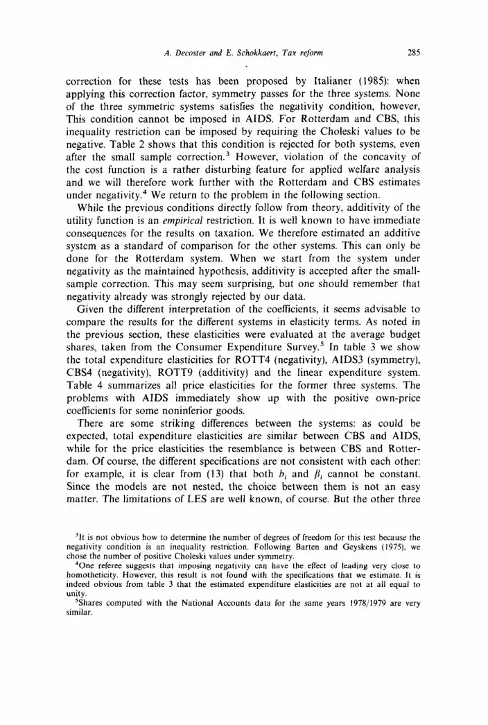
correction for these tests has been proposed by Italianer (1985): when applying this correction factor, symmetry passes for the three systems. None of the three symmetric systems satisfies the negativity condition, however, This condition cannot be imposed in AIDS. For Rotterdam and CBS, this inequality restriction can be imposed by requiring the Choleski values to be negative. Table 2 shows that this condition is rejected for both systems, even after the small sample correction.3 However, violation of the concavity of the cost function is a rather disturbing feature for applied welfare analysis and we will therefore work further with the Rotterdam and CBS estimates under negativity.4 We return to the problem in the following section.

While the previous conditions directly follow from theory, additivity of the utility function is an empirical restriction. It is well known to have immediate consequences for the results on taxation. We therefore estimated an additive system as a standard of comparison for the other systems. This can only be done for the Rotterdam system. When we start from the system under negativity as the maintained hypothesis, additivity is accepted after the small- sample correction. This may seem surprising, but one should remember that negativity already was strongly rejected by our data.

Given the different interpretation of the coefficients, it seems advisable to compare the results for the different systems in elasticity terms. As noted in the previous section, these elasticities were evaluated at the average budget shares, taken from the Consumer Expenditure Survey.’ In table 3 we show the total expenditure elasticities for ROTT4 (negativity), AIDS3 (symmetry), CBS4 (negativity), ROTT9 (additivity) and the linear expenditure system. Table 4 summarizes all price elasticities for the former three systems. The problems with AIDS immediately show up with the positive own-price coefficients for some noninferior goods.

There are some striking differences between the systems: as could be expected, total expenditure elasticities are similar between CBS and AIDS, while for the price elasticities the resemblance is between CBS and Rotter- dam. Of course, the different specilications are not consistent with each other: for example, it is clear from (13) that both bi and pi cannot be constant. Since the models are not nested, the choice between them is not an easy matter. The limitations of LES are well known. of course. But the other three

31t is not obvious how to determine the number of degrees of freedom for this test because the negativity condition is an inequality restriction. Following Barten and Geyskens (1975), we chose the number of positive Choleski values under symmetry.

*One referee suggests that imposing negativity can have the effect of leading very close to homotheticity. However, this result is not found with the specifications that we estimate. It is indeed obvious from table 3 that the estimated expenditure elasticities are not at all equal to unity.

%hares computed with the National Accounts data for the same years 197811979 are very similar.


___ FOOD BEVE TOBA CLOT RENT HEAT DURA HOUS PERS TRAN LEIS SERV

Rotterdam

0.654923 1.949600 0.484472 1.530910 0.013764 1.217049 3.016132 1.355625 1.387799 0.679130 0.682413 6.909038

Table 3

Total expenditure elasticities.

- Complete preference independence

AIDS CBS (Rotterdam)

0.597821 0.498945 0.996022 0.957932 1.106894 1 S70287

-0.205224 -0.228537 1.521314 1.493856 1.536456 1.887127 0.496411 0.48498 1 0.00023 1 1.567253 1.483557 0.191202 2.766841 2.752187 3.542886 0.533418 0.720986 0.969286 0.709662 0.902378 0.253219 0.746790 0.809635 0.659267 0.990877 0.923 185 0.600703 3.905373 4.412752 4.150863

LES

-)534531 1.561262 0.410965 0.732513 0.469456 1.087959 1.495286 0.820176 2.642756 1.287659 0.792828 7.361978

systems all are empirical approximations, and there are no convincing arguments to claim that one of them is superior within the range of observed values for the different variables. Each of the systems has its own supporters among demand specialists and the performance of the specifications seems to vary from case to case. This makes it all the more important to see whether the different estimates for the price elasticities lead to large differences in the estimates of the marginal cost of taxation, as presented in section 2.

4. Tax reform results with the different demand systems

We will proceed in three steps. First, we analyse the results for the case where the inequality aversion parameter e is zero. In that case eq. (6) reduces to:

MCI=- 1

, (16)

and the price effects play the dominant role in the explanation of differences between the MC;s. In this first step, we compare the results for the ‘best’ variants of the systems, i.e. ROTT4, AIDS3 and CBS4. As standards of comparison we also introduce ROTT9 (Rotterdam under complete preference independence), the linear expenditure system and the ‘easy’ practical solution where the estimation of demand systems is made unnecessary by the assumption


&ii = - 1

&ik = 0 , Vi#k. (17)

We will call this the ‘diagonal’ assumption. In a second step we stick to eq. (16), but we will compare the results for the different variants of the systems. We there return to the problem of the previous section about imposing the negativity condition. In the final step we consider what the consequences are of increasing e.

What matters for the tax reform problem is the ranking of the different marginal welfare costs. In fact, the numerical values of these costs are dependent on the normalization, chosen for the B”‘s. We will therefore

summarize our comparisons with Spearman rank correlation coefficients.

4.1. Comparison of results for the case e =O

The results for the case e=O are shown in table 5. For some commodities the estimates seem quite different between the systems, striking examples being ‘beverages’ and, especially, ‘services’. The results for the linear expenditure system differ considerably from these for the other systems. Among the flexible forms, the outlier is AIDS, which is not surprising given the positioe own-price elasticities for these commodities in that system. Remember that for both CBS and Rotterdam, negativity has been imposed. On the other hand, it is easily possible to draw some generally valid policy conclusions from table 5: one could say that the marginal welfare cost for increasing taxes on tobacco and transportation (where Belgium has now already important excise taxes) is high for all sets of estimates.

In table 5 we give, in parentheses, the estimated standard errors of the marginal costs6 These are small for the estimates based on the linear expenditure system. Yet they are relatively large with the other systems, at least for some commodities (not surprisingly beverages and services, but also tobacco). This implies that one has to be c”+‘. ‘11 ,,J when drawing conclusions

6Write eq. (6) as MC,= fi(c), where E is the vector of price elasticities. These price elasticities are the only stochastic components in eq. (6). The covariance matrix V of the marginal costs then has been computed through the first order-approximation [uij] = [2fJ&]‘V,[?f,/&], where V, is the covariance matrix of the price elasticities. Treating the budget shares as nonstochastic, this latter matrix can be calculated directly from the covariance matrix of the estimated coefficients for Rotterdam, AIDS and CBS. The DEMMOD program gives an estimate of this covariance matrix of the coefficients for the homogeneity variant. This is an asymptotically consistent estimator for the covariance matrices under symmetry and negativity. For the linear expenditure system, the elasticities are a nonlinear function of the estimated coefficients. Their covariance matrix then also has been computed through a first order-approximation.

Tab

le

4

Pri

ce e

last

icit

ies.

FO

OD

B

EV

E

TO

BA

C

LO

T

RE

NT

H

EA

T

DU

RA

H

OU

S

PE

RS

T

RA

N

LE

IS

SE

RV

FO

OD

B

EV

E

TO

BA

C

LOT

R

EN

T

HE

AT

D

UR

A

HO

US

P

ER

S

TR

AN

L

EIS

S

ER

V

FO

OD

B

EV

E

TO

BA

C

LO

T

RE

NT

H

EA

T

DU

RA

H

OU

S

PE

RS

T

RA

N

LE

IS

SE

RV

-0.6

7 -0

.38

0.20

-0

.14

- 0.

02

-0.2

5 -0

.39

0.22

0.

04

- 0.

09

-0.0

1 1.

00

-__-

-~~

- - 0.

46

-0.4

1 0.

03

-0.2

0 -

0.02

-0

.00

-0.5

3 0.

10

-0.1

8 -0

.22

-0.0

3 0.

55

- 0.

02

-0.1

4 -0

.01

0.09

0.

01

-0.0

9 -0

.12

- 0.

08

-0.0

1 -

0.05

-

0.03

-0

.12

RO

TT

4 ~

_~~

__~

~~

~~

_~__

___~

~~

_~~

~~

_~_~

~__

P

0.

01

0.02

-0

.14

- 0.

05

0.03

0.

05

0.05

-

0.06

-0

.00

0.12

b

- 0.

02

0.25

-0

.33

- 0.

94

-0.2

7 -0

.24

- 0.

05

-0.8

0 -0

.32

-0.0

1 -0

.01

-0.0

3 -0

.01

0.10

-0

.17

0.07

-

0.02

-0

.65

0.09

-0

.02

-0.0

9 0.

12

-0.2

9 -0

.25

0.01

0.

03

-0.0

1 -

0.07

-

0.03

-0

.17

-0.2

4 -

1.00

-

1.80

-0.2

5 -0

.27

- 0.

02

0.67

0.

05

0.10

0.

02

- 0.

03

-0.3

6 -

0.05

-0

.16

-0.7

8 -

0.05

0.

23

-0.0

9 -0

.23

-0.1

1 0.

08

0.02

-0

.12

-0.3

8 -

1.52

AID

S3

- 0.

09

0.23

-0

.01

0.02

-0

.02

0.03

-

0.96

-

0.06

-

0.05

-0

.01

-0.5

0

- 0.

05

0.62

-0

.19

0.01

-

0.06

-0

.25

-0.1

3 -0

.28

- 0.

06

0.00

-0

.67

___

-0.0

5 -0

.01

-0.0

1 -

0.04

0.

19

0.07

0.

25

-0.5

6 0.

20

-0.2

0 -0

.44

-0.1

5 0.

06

-0.0

8 -0

.65

-0.3

1 -

0.07

-0

.02

- 0.

05

- 0.

40

-0.1

0 -0

.02

0.11

-0

.21

-0.1

7 0.

06

0.01

-0

.61

-0.0

3 0.

22

- 0.

08

0.37

-

0.05

0.

15

-0.3

3 0.

03

0.03

0.

02

0.06

0.

17

0.05

-0

.14

-0.0

4 -0

.15

-0.2

2 -0

.36

-1.0

8 -1

.74

0.06

-0

.04

0.01

-

0.04

-0

.12

-0.2

0 -0

.36

-0.0

4 -0

.12

0.06

-0

.00

0.67

0.

51

0.75

0.

33

0.09

0.

11

- 0.

05

-0.2

5 -0

.04

0.00

-

0.07

0.

05

0.02

0.

14

-0.4

1 0.

03

- 0.

09

-0.2

9 -0

.44

-0.0

5 0.

13

0.02

-0

.26

-0.1

7 -0

.16

0.25

-0

.02

-0.1

3 -0

.14

-0.2

8 -0

.21

- 0.

06

0.20

-0

.13

-0.1

8 0.

06

- 0.

03

-0.0

6 -0

.69

0.04

-0

.37

-0.1

3 -

0.02

-0

.10

- 1.

23

- 3.

79

- 1.

12

0.77

1.

73

-0.4

0 -

0.25

0.

12

-0.6

9 -0

.06

-0.1

4 0.

07

-0.0

2 -0

.28

- 0.

02

-0.1

6 -

0.43

-0

.32

-0.1

1 -0

.21

- 0.

08

-0.5

6 -

0.02

-

0.02

-0

.19

1.16

-

1.32

0.03

0.

06

4 9

0.22

-0

.05

3

-1.2

2 -0

.28

-0.1

1 -0

.10

- 0.

03

-0.0

6 0.

01

-0.1

7 -0

.72

- 0.

47

-0.5

2 -0

.41

-0.0

1 0.

18

- 0.

07

0.18

-0

.15

0.05

0.

17

2.40

0.01

c:

-0

.15

? :: -

0.06

%

- 0.

02

g -0

.00

p.

-0.1

5 pl

-0

.14

v1

E

- 0.

07

%

0.16

-0

.06

tz

“2

- 1.

51

~__

____

i?

CB

S4

- 0.

08

0.03

0.

09

-0.1

4 -0

.04

-0.1

1 0.

04

-0.2

1 0.

12

0.20

-0

.33

-0.0

9 -0

.27

0.09

0.

31

- 0.

92

-0.0

5 -0

.24

0.07

0.

09

0.52

0.

05

- 0.

03

-0.7

9 -0

.32

0.04

-0

.00

0.01

-0

.03

- 0.

02

- 0.

06

-0.1

4 -0

.00

-0.0

7 0.

04

-0.0

5 -0

.01

0.06

-0

.21

-0.3

3 -

0.02

-

0.00

-0

.14

-0.0

2 -0

.11

-0.6

1 -0

.10

-0.4

7 -0

.02

0.11

0.

22

0.12

0.

25

0.04

0.

11

-0.8

5 0.

01

0.06

-0

.31

-0.1

2 -0

.04

0.13

-0

.13

0.02

-0

.01

0.02

-0

.05

-0.1

9 0.

13

-0.1

0 0.

00

- 0.

07

- 0.

06

-0.1

9 -0

.01

-0.1

5 -0

.03

- 0.

03

-0.0

1 -0

.69

-0.7

5 -0

.25

-0.7

0 -0

.31

FOO

D

-0.2

8 B

EV

E

-0.7

0 T

OB

A

0.58

C

LO

T

-0.0

0 R

EN

T

-0.1

4 H

EA

T

-0.3

2 D

UR

A

-0.7

2 H

OU

S 0.

24

PER

S -

0.05

T

RA

N

- 0.

05

LE

IS

-0.1

3 SE

RV

-

0.60

~__

_ 0.

01

0.01

0.

37

-0.2

3 -0

.01

-0.0

7 -0

.02

-0.2

6 -0

.23

-0.1

2 0.

01

-0.0

4

0.01

-

0.03

0.

06

-0.0

1 -

0.06

-0

.54

- 0.

06

-0.1

4 0.

01

-0.0

6 -0

.44

- 0.

08

-0.0

4 -

0.43

-0

.48

-0.1

3 -0

.29

0.03

-0

.50

- 0.

02

-0.0

4 -0

.22

0.37

-

0.74

___-

- 0.

01

0.02

0.

04

-0.0

5 0.

00

-0.0

1 -

0.07

-

0.09

0.

03

0.07

-

0.03

-0

.65


Table 5

MC,‘s and rankings for e=O.

Commo- dity DIAGONAL ROTT4 AIDS3 CBS4 ROTT9

FOOD

BEVE

TOBA

CLOT

RENT

HEAT

DURA

HOUS

PERS

TRAN

LEIS

SERV

1.0658

1.5236

3.1632

1.1783

1.0085

1.1571

1.1803

1.0773

1.0829

1.4715

1.1319

1.0146

10

2

I

5

12

6

4

9

8

3

7

11

1.1261 8 1.1648 5 1.1183 8 1.1323 11 1.1544 8 (0.0439) (0.0501) (0.0456) (0.0444) (0.0022)

1.2429 3 0.9438 12 1.0310 11 1.3759 2 1.5235 1 (0.4494) (0.2764) (0.3262) (0.5507) (0.0636)

2.7963 1 1.1548 6 2.7411 1 1.9117 1 1.4901 2 (3.2585) (0.5929) (3.3028) (1.5230) (0.0318)

1.1336 7 1.1106 8 1.1297 7 1.1790 6 1.1499 9 (0.0539) (0.0552) (0.0565) (0.0584) (0.0075)

1.1476 6 1.0893 9 1.1500 5 1.1812 4 1.0603 12 (0.0443) (0.0425) (0.0469) (0.0469) (0.0003)

1.2301 4 1.2316 4 1.2294 3 1.1734 7 1.1304 10 (0.0705) (0.0754) (0.0743) (0.0641) (0.0096)

1.0584 11 0.9868 11 1.0759 9 1.1799 5 1.1880 7 (0.1280) (0.1187) (0.1395) (0.1591) (0.0165)

1.1084 9 1.0289 10 1.0494 10 1.1385 10 1.3246 3 (0.4671) (0.4293) (0.4416) (0.4928) (0.0053)

1.0930 10 1.1396 7 1.1434 6 1.1704 8 1.2155 6 (0.1580) (0.1832) (0.1824) (0.1812) (0.0152)

1.3574 2 1.3677 1 1.2774 2 1.2462 3 1.2610 5 (0.1187) (0.1285) (0.1108) (0.1000) (0.0335)

1.2071 5 1.2589 3 1.1745 4 1.1689 9 1.1158 11 (0.1292) (0.1498) (0.1290) (0.1211) (0.0059)

0.8096 12 1.3633 2 0.8998 12 0.9277 12 1.3149 4 (0.3818) (1.1549) (0.4974) (0.5014) (1.1774)

LES

Ranking of commodities

Highest TOBA TOBA TRAN TOBA TOBA BEVE marginal BEVE TRAN SERV TRAN BEVE TOBA welfare TRAN BEVE LEIS HEAT TRAN HOUS cost DURA HEAT HEAT LEIS RENT SERV

CLOT LEIS FOOD RENT DURA TRAN HEAT RENT TOBA PERS CLOT PERS LEIS CLOT PERS CLOT HEAT DURA PERS FOOD CLOT FOOD PERS FOOD

Lowest HOUS HOUS RENT DURA LEIS CLOT marginal FOOD PERS HOUS HOUS HOUS HEAT welfare SERV DURA DURA BEVE FOOD LEIS cost RENT SERV BEVE SERV SERV RENT


Table 6

Rank correlation between demand models (e=O).

DIAGONAL ROTT4 AIDS3 CBS4 ROTT9 LES

DIAGONAL l.OOOQ ROTT4 0.6224 1.0000 AIDS3 -0.1329 0.1608 1.0000 CBS4 0.3427 0.6923 0.4406 1.0000 ROTT9 0.7413 0.7133 -0.3147 0.4615 1.0000 LES 0.4545 0.0979 -0.1958 -0.3217 0.2238 1.0000

about welfare-improving directions of tax reform. For CBS4, for example, there is a probability of about 0.30 that one commits an error by stating that the marginal cost of tobacco is larger than the one of services (one-sided t- test). However, as noted by Ahmad and Stern (1987, p. 301), if the estimated marginal cost of taxing commodity i is larger than the estimated marginal cost of taxing commodity j, then the expected change in welfare from a switch into j is positive; and if the distribution is symmetric, the probability of an increase in welfare is above 50 percent. It therefore still makes sense to look at the rankings of the marginal welfare costs.

The information for the different systems is summarized in table 6, where we give rank correlation coefficients. The linear expenditure and AIDS- systems obviously are outliers. The affinity of Rotterdam and CBS is clear. It is striking also that the ‘simple’ solutions (DIAGONAL and ROTT9) are not completely divergent from the more complex systems. It is probably fair to conclude that the differences between the results are not as large as could be expected when considering table 4. There is some truth in Ahmad and Stern’s (1984, p. 293) suggestion that this might be explained by the fact that all the demand effects are summed to compute (16). On the other hand, our results also suggest that the practitioner who would use information from one system only (e.g. AIDS under symmetry) cannot be confident that his results are not influenced heavily by this (more or less arbitrary) choice of system. We will now see whether this result is due to the fact that we compare AIDS under symmetry with the other systems under negativity.

4.2. Results for the different variants (e = 0)

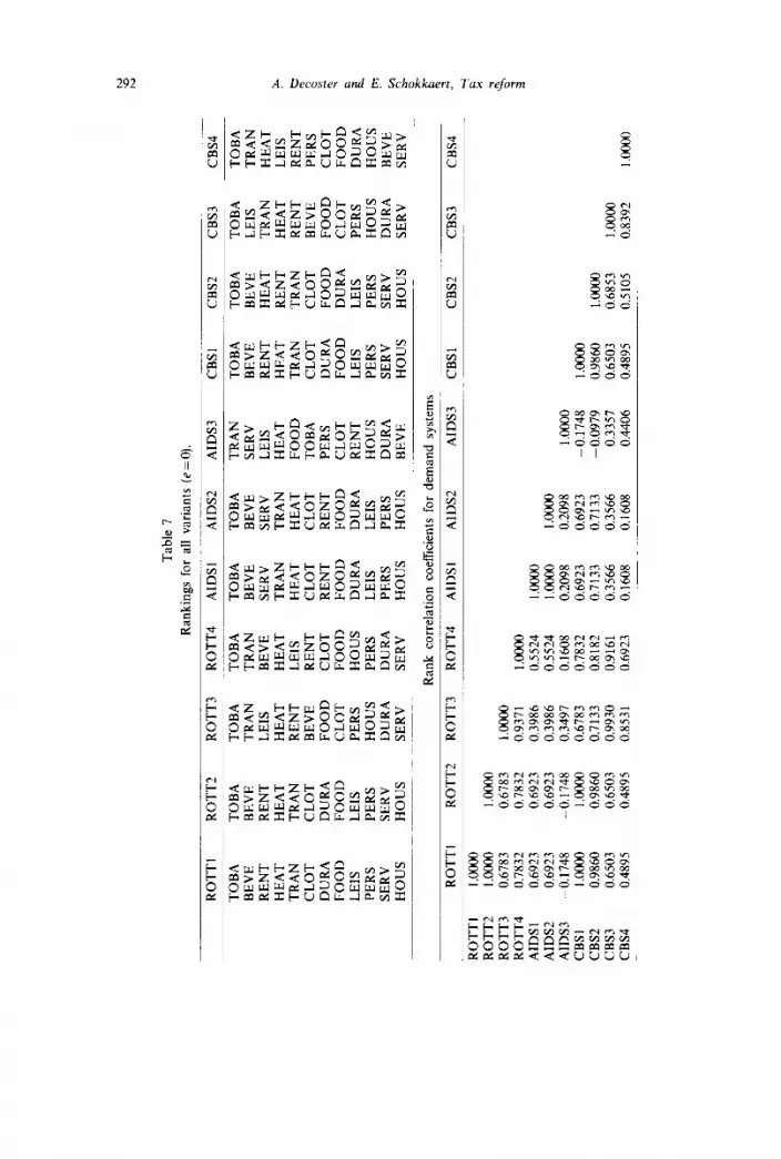
Table 7 shows the rankings of welfare costs for the different variants of the flexible functional form systems and the corresponding rank correlation coefficients. The suffixes 1 to 4 refer to the variants ‘free’, ‘under homogeneity’, ‘under homogeneity and symmetry’, and ‘under homogeneity, symmetry and negativity’, respectively. We see that the divergent behaviour of AIDS is also present when we compare AIDS3 with CBS3 and ROTT3. In fact, table 7 suggests some further interesting conclusions.

Tab

le 7

Ran

kin

gs

for

all

vari

ants

(e=

O).

RO

TT

I R

OT

T2

RO

TT

3 R

OT

T4

AID

S1

AID

S2

AID

S3

CB

S1

CB

S2

CB

S3

CB

S4

TO

BA

T

OB

A

TO

BA

T

OB

A

TO

BA

T

OB

A

TR

AN

T

OB

A

TO

BA

T

OB

A

TO

BA

B

EV

E

RE

NT

H

EA

T

TR

AN

C

LO

T

DU

RA

F

OO

D

LE

IS

PE

RS

S

ER

V

HO

US

BE

VE

R

EN

T

HE

AT

T

RA

N

CL

OT

D

UR

A

FO

OD

L

EIS

P

ER

S

SE

RV

H

OU

S

TR

AN

L

EIS

H

EA

T

RE

NT

B

EV

E

FO

OD

C

LO

T

PE

RS

H

OU

S

DU

RA

S

ER

V

TR

AN

B

EV

E

BE

VE

S

ER

V

BE

VE

S

ER

V

SE

RV

L

EIS

H

EA

T

TR

AN

T

RA

N

HE

AT

L

EIS

H

EA

T

HE

AT

F

OO

D

RE

NT

C

LO

T

CL

OT

T

OB

A

CL

OT

R

EN

T

RE

NT

P

ER

S

FO

OD

F

OO

D

FO

OD

C

LO

T

HO

US

D

UR

A

DU

RA

R

EN

T

PE

RS

L

EIS

L

EIS

H

OU

S

DU

RA

P

ER

S

PE

RS

D

UR

A

SE

RV

H

OU

S

HO

US

B

EV

E

Ran

k

corr

elat

ion

co

effi

cien

ts f

or d

eman

d sy

stem

s

BE

VE

R

EN

T

HE

AT

T

RA

N

CL

OT

D

UR

A

FO

OD

L

EIS

P

ER

S

SE

RV

H

OU

S

BE

VE

H

EA

T

RE

NT

T

RA

N

CL

OT

F

OO

D

DU

RA

L

EIS

P

ER

S

SE

RV

H

OU

S

LE

IS

TR

AN

H

EA

T

RE

NT

B

EV

E

FO

OD

C

LO

T

PE

RS

H

OU

S

DU

RA

S

ER

V

RO

TT

l l.

GQ

OO

R

OT

T2

l.oo

oo

RO

TT

3 0.

6783

R

OT

T4

0.78

32

AID

S1

0.69

23

AID

S2

0.69

23

AID

S3

-0.1

748

CB

S1

1.00

00

CB

S2

0.98

60

CB

S3

0.65

03

CB

S4

0.48

95

RO

TT

l R

OT

TZ

R

OT

T3

RO

TT

4 A

IDS

1 A

IDS

2 A

IDS

3 C

BS

1 C

BS

2 C

BS

3

1.00

00

0.67

83

0.78

32

0.69

23

0.69

23

-0.1

748

1.00

00

0.98

60

0.65

03

0.48

95

1.oo

oo

0.93

71

0.39

86

0.39

86

0.34

97

0.67

83

0.71

33

0.99

30

0.85

31

1.00

00

0.55

24

l.G

QO

O

0.55

24

l.cO

oo

l.G

QO

O

0.16

08

0.20

98

0.20

98

1.00

00

0.78

32

0.69

23

0.69

23

-0.1

748

0.81

82

0.71

33

0.71

33

- 0.

0979

0.

9161

0.

3566

0.

3566

0.

3357

0.

6923

0.

I608

0.

1608

0.

4406

1.00

00

0.98

60

0.65

03

0.48

95

1.00

00

0.68

53

0.51

05

1.00

00

0.83

92

TR

AN

H

EA

T

LE

IS

P

RE

NT

P

ER

S

?

CL

OT

Y

?

FO

OD

5

DU

RA

2 %

H

OU

S

BE

VE

h

G

l S

ER

V

E

%

K

CB

S4

“2

1.00

00


Free estimates of the different systems lead to very similar rankings of the welfare costs. Imposing homogeneity does not change this picture drastically. In fact, these two variants could be seen as exercises of curve fitting, while homogeneity only imposes one restriction per equation. Symmetry, however, leads to pronounced changes in the rankings, even for the same system: compare ROTT2 and ROTT3, AIDS2 and AIDS3, and CBS2 and CBS3. At the same time, differences between the different systems also grow larger. There still is a close connection between CBS3 and ROTT3, however.

This may be the place to return to a question, raised earlier: Should one

impose the theoretical restrictions ? In our case, at least three possible positions can be taken. A tirst one could be called the theoretical position. The theoretician will argue that welfare-economic applications run into deep trouble when estimated demand parameters are not consistent with a concave cost function. He will point out that there are so many data limitations and remaining theoretical problems7 that one should not attach too much attention to the statistical rejection of the negativity condition. In our case, the theoretician has to face the problem that to a certain extent results will be dependent on the choice of specification. Either he will have to compare different systems in order to draw conclusions which hold for all (as is possible with our results), or he will have to argue on theoretical grounds that one system is superior. A second position could be called the statisrical one. Someone holding this position will not want to impose theoretical restrictions if they are rejected by the data. In our case, he will stick to the symmetry versions,’ and he will have to face the same choice problem as the theoretician. A third position is the pragmatic one. The pragmatist will not like to be faced with a choice between different systems. Like the theoretician he will point to the many problems (both theoretical and practical) arising when estimating a fully-fledged complete demand system. He will argue that we do not need accurate estimates of all cross-price effects and that to apply (16) only the sum of these effects is necessary. Why bother about the precise estimation of cross-price effects if we can only estimate them conditional upon the ‘arbitrary’ choice of system? After all, one can have doubts about the validity of the theory. The pragmatist probably will be happy with the finding that a free curve-fitting exercise (even after imposing the homogeneity condition) yields results which are rather insensi- tive to the exact specification used and could prefer these nonsymmetric estimates.

While endorsing the theoretical position ourselves, we feel that more

‘For an overview see Deaton and Muellbauer (1980a, pp. 78-82). *Note that Wibaut (1987) in his empirical application for Belgium uses estimates from a

Rotterdam system with symmetry imposed, but with a positive diagonal element in the Slutsky matrix. He does not explain why he uses that variant.


Table 8

Rank correlations between demand systems.

Value of e Correlation between 0.0 0.1 0.5 I.0 2.0 5.0 10.0

CBS4ZERO 0.1888 0.1329 0.1678 0.2937 0.4545 0.6593 0.8531 CBS4-DIAGONAL 0.3427 0.3427 0.3776 0.4895 0.5035 0.6154 0.7692 CB!+l-ROTT4 0.6923 0.6923 0.6923 0.7823 0.8392 0.8462 0.9301 CBShAIDS3 0.4406 0.4406 0.3916 0.3916 0.3846 0.4545 0.6224 CBS4ROTT9 0.4615 0.4615 0.5804 0.6084 0.7413 0.8042 0.909 1 CBM-LES -0.3217 -0.3217 - 0.2937 - 0.2448 -0.0769 0.3427 0.5944 ROTT&AIDS3 0.1608 0.1608 0.1119 0.2308 0.2937 0.3427 0.4825

_

Table 9

Rankings for e=2.

DIAGONAL ROTT4 AIDS3 ____

CBS4 ROTT9 LES

1 2 3 4 5 6 I 8 9

10 11 12 -

ZERO

HEAT FOOD TOBA BEVE PERS SERV RENT LEIS CLOT HOW DURA TRAN

TOBA TOBA SERV TOBA TOBA BEVE BEVE HEAT TRAN HEAT BEVE TOBA TRAN TRAN HEAT TRAN HEAT SERV HEAT BEVE LEIS FOOD PERS HOUS CLOT LEIS FOOD PERS RENT PERS DURA FOOD TOBA RENT TRAN FOOD FOOD RENT PERS LEIS FOOD TRAN LEIS PERS RENT CLOT CLOT HEAT PERS CLOT CLOT BEVE LEIS DURA HOUS HOUS HOUS DURA DURA CLOT SERV DURA BEVE HOUS HOUS LEIS RENT SERV DURA SERV SERV RENT

experience with demand systems will be needed before convincing argumentation for any of these positions.

4.3. Increasing the inequality aversion

one can give a fully

Table 8 shows the effects of increasing the inequality aversion parameter e. In this table we use CBS4 as the main standard of comparison and add a variant ‘ZERO’ which simply assumes that .Q~=O, Vk, i, and hence neglects all changes in demand. Table 9 contains the rankings for e=2, which seems to be a ‘reasonable’ value [see Stern (1977)].

For e=2, there still are important differences between the results with the different systems, while as before it is possible at the same time to draw some stable policy conclusions. Table 8 clearly shows that the differences become smaller when e increases. This result is opposite to the one found by Ray (1986) in his computation of ‘optimal’ taxes. The explanation is obvious,


however. When e increases, considerations of distributive justice get a relatively larger weight in (5) and (6). In fact, these considerations become irrelevant when e=O [see (16)]. In the framework of tax reform (in contrast to optimal taxation), justice considerations are captured by actual obser- vations of consumption patterns [the numerator in (6)] and, hence, completely independent of the elasticity estimates. For an analysis of tax reform, increasing e therefore amounts to increasing the relative weight attached to actual consumption. A striking illustration of this phenomenon is the high correlation between the results for CBS4 and the results for DIAGONAL and (even!) ZER0.9

5. Conclusion

A comparison of the results with the different systems shows that it is possible to draw relevant policy conclusions that hold for all of them. This similarity occurs despite the differences in the matrices of estimated expenditure and price elasticities. From that point of view, it is possible to corroborate the suggestion that the sensitivity to the specification of the demand system is less severe for a tax reform exercise than it is for the calculation of optimal tax rates. This does not mean, however, that the exclusive use of one system always leads to reliable results. Some differences remain large and a sensitivity analysis seems to be advisable. Increasing the inequality aversion implies that a relatively larger weight is given to observed consumption patterns. The choice of demand system therefore becomes less crucial.

It is remarkable how strongly the rankings of the marginal welfare costs are affected by imposing the restriction of symmetry of the Slutsky matrix. Without this integrability condition, the different systems yield very similar results. This could be interpreted by a pragmatist as implying that the estimates of the cross-price effects are heavily influenced by the mathematical straitjacket of the chosen specification, and that the symmetrical estimate of the Slutsky matrix is not really informative about reality. Then why not use the estimates under homogeneity? Surely, more work about specification and estimation of complete demand systems will be necessary if one wants to formulate a completely convincing answer to this pragmatical critique.

‘Increasing e, i.e. increasing the relative weight attached to actual consumption (a nonstochastic variable), also leads to a considerable decrease in the estimated standard errors of the marginal costs.

References

Ahmad, E. and N. Stern, 1984, The theory of reform and Indian indirect taxes, Journal of Public Economics 25, 259-298.


Ahmad, E. and N. Stern, 1987, Alternative sources of government revenue, in: D. Newbery and N. Stern, eds., The theory of taxation for developing countries (Oxford University Press) 281-332.

Atkinson, A.B., 1977, Optimal taxation and the direct versus indirect tax controversy, Canadian Journal of Economics IO, 590-606.

Barten, A.P. and E. Geyskens, 1975, The negativity condition in consumer demand, European Economic Review 6, 227-260.

Bewley, R., 1986, Allocation models: Specification, estimation and applications (Ballinger, Cambridge).

Christensen, L.R., D.W. Jorgenson and L.J. Lau, 1975, Transcendental logarithmic utility function, American Economic Review 65, 367-383.

Deaton, A., 1981, Optimal taxes and the structure of preferences, Econometrica 49, 1245-1260. Deaton, A., 1987, Econometric issues for tax design in developing countries, in: D. Newbery and

N. Stern, eds., The theory of taxation for developing countries (Oxford University Press) 92-l 13.

Deaton, A. and J. Muellbauer, 1980a, Economics and consumer behavior (Cambridge University Press).

Deaton, A. and J. Muellbauer, 1980b, An almost ideal demand system, American Economic Review 70, 312-326.

Decoster, A. and E. Schokkaert, 1989, Equity and efficiency of a reform of Belgian indirect taxes, Recherches Economiques de Louvain 55, 155-176.

Fisher, F., 1987, Household equivalence scales and interpersonal comparisons, Review of Economic Studies 54, 519-524.

Italianer, A., 1985, A small-sample correction for the likelihood ratio test, Economics Letters 19, 315-317.

Keller, W.J. and J. Van Driel, 1985, Differential consumer demand systems, European Economic Review 27, 3755390.

Laitinen, K., 1978, Why is demand homogeneity so often rejected?, Economics Letters 1, 187-191.

Paraire-Laguesse, Y. et al., 1986, De weerslag van de indirecte belastingen op de verdeling van de gezinsinkomens in Belgii, Documentatieblad van het Ministerie van Financien van Belgii 7-8, 9-32.

Ray, R., 1986, Sensitivity of ‘optimal’ commodity tax rates to alternative demand functional forms, Journal of Public Economics 31, 253-268.

Stern, N., 1977, The marginal valuation of income, in: M. Artis and A. Nobay, eds., Studies in modern economic analysis (Blackwell, Oxford) 209-254.

Theil, H., 1975/1976, Theory and measurement of consumer demand I and II (North-Holland, Amsterdam).

Wibaut, S., 1987, A mode) of tax reform for Belgium, Journal of Public Economics 32, 53-77.

Documents

Tax reform results with different demand systems