Discrete Applied Mathematics 29 (1990) 171-185

North-Holland

171

THE BASIC ALGORITHM FOR PSEUDO-BOOLEAN PROGRAMMING REVISITED

Yves CRAMA

Department of Quantitative Economics, University of Limburg, Postbus 616, 6200 MD Maastricht, The Netherlands

Pierre HANSEN

RUTCOR, Rutgers University, P.O. Box 5062, New Brunswick, NJ 08903, USA

Brigitte JAUMARD

GERAD and Department of Applied Mathematics, .&Cole Polytechnique de MontrPaI, Campus de I’Universite’ de MontrPal, Case Postale 6079, Succursale “A” Mont&al, QuPbec, Canada H3C3A7

Received 10 November 1988

Revised 10 April 1989

The basic algorithm of pseudo-Boolean programming due to Hammer and Rudeanu allows to

minimize nonlinear O-l functions by recursively eliminating one variable at each iteration. We

show it has linear-time complexity when applied to functions associated in a natural way with

graphs of bounded tree-width. We also propose a new approach to the elimination of a variable

based on a branch-and-bound scheme, which allows shortcuts in Boolean manipulations.

Computational results are reported on.

1. Introduction

The basic algorithm for pseudo-Boolean programming was originally proposed

by Hammer, Rosenberg and Rudeanu 25 years ago [ 10, 111. A streamlined form due

to Hammer and Rudeanu is presented in their book “Boolean Methods in Opera-

tions Research and Related Areas” [12]. This algorithm determines the maximum

of a nonlinear function in O-l variables, or pseudo-Boolean function, by recursively

eliminating variables. Following the dynamic programming principle, local op-

timality conditions are exploited so as to produce at each iteration a function depen-

ding on one less variable, but having the same optimal value as the previous one.

No systematic effort for programming this method appears to have been made.

Possible reasons for this are the relative sophistication required to implement

Boolean manipulations of formulas, and the large memory space necessary for the

storage of intermediary results. Hence, with the advent of new methods, the basic

algorithm has progressively fallen into oblivion during the last decade.

0166-218X/90/$03.50 0 1990 - Elsevier Science Publishers B.V. (North-Holland)

172 Y. Crama et al.

For several reasons, this seems unwarranted. First, while the basic algorithm may

not be the most efficient for maximizing arbitrary pseudo-Boolean functions, it

might be the case that it is very well adapted to the maximization of functions

belonging to particular classes. For instance, several polynomial algorithms

(see [6, 8, 15]), which are in fact subsumed by the basic algorithm, have been

recently proposed for the maximization of quadratic pseudo-Boolean functions

associated with trees or series-parallel graphs. Second, some steps of the basic

algorithm might be simplified. Third, the explosive development of algorithm

design and data structuring renders the programming of complex combinatorial

methods much easier to do efficiently than even a decade ago. Fourth, the

availability of powerful computers with large internal memory substantially

increases the size of potentially solvable problems.

In this paper, we reconsider the basic algorithm both from the theoretical and

from the computational point of view. We recall the details of the basic algorithm

in Section 2, and we present the variant of it we will consider in the sequel

of the paper. In Section 3, we establish that the basic algorithm has linear-time

complexity when applied to functions associated in a natural way with graphs of

bounded tree-width.

In Section 4, we propose a new approach to the elimination of a variable, based

on a branch-and-bound scheme. This subroutine is directly applied to the subfunction

defined by the terms containing the variable to be eliminated, and several steps of

the basic algorithm, using Boolean manipulations, are thus cut short. We study in

Section 5 the data structures required for the representation of pseudo-Boolean

functions, and for an efficient implementation of the algorithm. We also report on

computational experiments.

2. The basic algorithm

A pseudo-Boolean function is a real-valued function of O-l variables. Any such

function can be (nonuniquely) expressed as a polynomial in its variables x1, x2, . . . ,x,

and their complements x1 = 1 -xl, x2 = 1 -x2, . . . , xn = 1 - x, , of the general form:

f(x,,x2, ***1 x,) = f c, n x,y

f=l jE T(t)

where m is the number of terms of the polynomial, T(t) is a subset of { 1,2, . . . , n}

(t=1,2, . ..) m), OZjtE (0, l} (t’ 1,2, . . . . m; Jo T(t)), and x1=x, x0=x.

We present now the scheme of the basic algorithm of Hammer, Rosenberg and

Rudeanu, for maximizing over { 0,l)” a pseudo-Boolean function in polynomial

form.

Let fi be the function to be maximized, and write:

f,(xiYx*, ...? x,) = x,g,(x,,xs, ..-,xn)+hi(x2,xj, . . ..xn).

The basic algorithm for pseudo-Boolean programming revisited 173

where the functions g, and ht do not depend on x1. Clearly, there exists a maximizing

point of fi , say (x;“,x,*, . . . , x,*), such that x;“=l if g,(x:,x:,...,x,*)>O, and such

thatx~=Oifg,(x~,x~,..., x,*) I 0. This leads us to define a function w1 (x2, x3, . . . ,x,),

such that wl(xz,xs, . . ..x.J=gl(x2,x3, . . ..x.,) if gt(+,xs, . . ..x.J>O, and wt(x2, x3, . . . ,x,J = 0 otherwise. Assume that a polynomial expression of ly, has been ob-

tained. Letting f2 = I,V~ + h,, we have thus reduced the maximization of the original

function in n variables to the maximization of f2, which only depends on the n - 1

variables x2,x3, . . . ,x,.

Continuing this elimination process for x2, x3, . . . ,x, _ I , successively, we produce

two sequences of functions fi, f2, . . . , f, and v/~, w2, . . . , tyn_, , where fi depends on

n - i + 1 variables. A maximizing point (XT, XT, . . . ,x,*) of fi can then easily be

tracked back from any maximizer x,* off,, using the recursion:

xF= 1 if and only if t,uj(xiy”,,,x,*f2 ,..., x,*)>O (i= 1,2 ,..., n-1).

Obviously, the efficiency of this algorithm hinges critically on how difficult the

polynomial expressions of v/,, w2, . . . , (I/~ _ 1 are to obtain. And, as already observed

in [12], this can in turn be influenced by the elimination order chosen for the

variables. We return to this issue in Section 3.

Notice that the original version of the basic algorithm is slightly more complex

than the one presented above. We summarize it here to allow comparison with the

algorithm of Section 4. A logical expression @t for x1 is first obtained by: (i)

linearizing g, (x2, x3, . . . , x,), by replacing products of variables by new variables yj

(i= 1,2, . . . . p), (ii) computing the characteristic function @t of the linear inequality

g*(Y,,Y,,..., yp)> 0 (by definition, o,(y) is a Boolean function equal to 1 if

gl(y)>O and equal to 0 otherwise), (iii) eliminating the y, from @I and simplifying

it through Boolean operations. Then, (iv) x1 is replaced by Q1 in x,g,(x,,x,, . . . ,x,)

and pseudo-Boolean simplifications are made, yielding wI(x~, ~3, . . . , x,). The

values XT are recursively obtained from @;(xT+ t, xi*, 2, . . . , x,*). All optimal solutions

may be obtained by analyzing the equality g, (y,, y2, . . . , yP) = 0 in a similar way as

the inequality g,(y,, y,, . . . , yJ > 0 above, and introducing parameters.

3. Pseudo-Boolean functions with bounded tree-width

We use the graph-theoretic terminology of Bondy and Murty 141. All graphs in

this paper are simple and undirected. A vertex v is simplicial in a graph G if the

neighbors of v induce a complete subgraph of G. For k20, a k-perfect elimination scheme of a graph G is an ordering (u,, v2, . . . , u,) of its vertices, such that v, is

simplicial and has degree k in the subgraph Gj of G induced by { Vj, Uj+ t, . . . , v,}

(j= 1,2 , . . . , n - k). A graph is a k-tree if it has a k-perfect elimination ordering. A

partial k-tree is any graph obtained by deleting edges from a k-tree.

Since the complete graph on n vertices is an (n - 1)-tree, every graph is also a

174 Y. Crama et al.

partial (n-1)-tree. The tree-width of a graph is the smallest value of k for which this graph is a partial k-tree (see [l, 191 for equivalent definitions). For instance, trees and forests have tree-width at most 1, and series-parallel graphs have tree-width at most 2. Arnborg, Corneil and Proskurowski [2] proved that determining the tree-width of a graph is NP-hard. However, for every fixed k, there is a polynomial algorithm to decide if a graph has tree-width k [l, 191. In fact, the algorithm in [l] is constructive: if G has tree-width k, then the algorithm returns a k-perfect elimination scheme of some k-tree containing G as a subgraph. For brievity, we will refer to such a scheme as a k-scheme of G.

Let us now consider a pseudo-Boolean function f(xl,xz, . . . ,x,) expressed in polynomial form. The co-occurrence graph of f, denoted G(f), has vertex set V= {x1,x2, . ..) xn}, with an edge between Xi and Xj (ifj) if these variables occur simultaneously, either in direct or in complemented form, in at least one term of f. The tree-width off is the tree-width of G(f).

Remark. Strictly speaking, the graph G(f) and its tree-width are not completely determined by f, but only by the particular expression considered for f. Nevertheless, it will be a convenient, and harmless abuse of language to speak of the graph and the tree-width off.

For every fixed k, there is a polynomial-time algorithm to decide whether a given pseudo-Boolean function f(x1,x2, . . . , x,) has tree-width at most k. Moreover, using the algorithm of Arnborg et al. [2], the variables of such a function can always be relabelled, so that (x1,x2, . . . ,x,) is a k-scheme of G(f).

Theorem. For every fixed k, the basic algorithm can be implemented to run in O(n) time on those pseudo-Boolean functions f (x1, x2, . . . ,x,,>, expressed in polynomial form, for which (x1,x2, . . . , x,,) is a k-scheme of G(f).

Proof. Fix k, and let f(xI,x2, . . . . x,) be as in the statement of the theorem.

(1) In order to carry out efficiently the computations required by the basic algorithm, we need a little bit of data structuring. Namely, we need a list re- presentation of f consisting, for each variable Xi, of a list of the terms of f containing Xi but not x1, ~2, . . . , Xi _ 1, together with the coefficients of these terms (i= 1,2, . . . . n). This representation can be obtained easily. Indeed, since xi has degree at most k in G(f), it is contained in at most 2. 3k terms of G(f). Similarly, each variable xi occurs in at most 2 . 3k terms not containing x1,x,, . . . ,Xi_ 1 .

Therefore, f has at most 2. 3kn terms, i.e., O(n) terms. Also, since G(f) has no clique on k + 2 vertices, all terms off have at most k + 1 variables. It follows that a list representation off can be obtained in time O(n), by scanning through the terms off.

(2) Now, we show that, when applying the basic algorithm to f, =f, we can

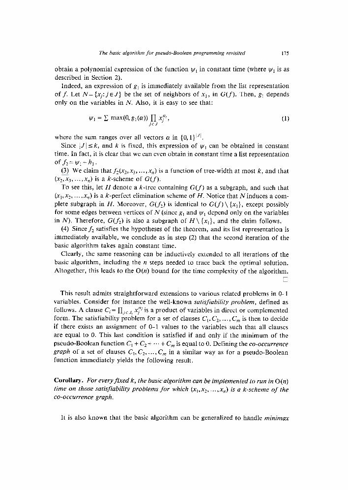
The basic algorithm for pseudo-Boolean programming revisited 175

obtain a polynomial expression of the function w1 in constant time (where w1 is as

described in Section 2).

Indeed, an expression of g, is immediately available from the list representation

off. Let N= (xj: j E J} be the set of neighbors of xi, in G(f). Then, gl depends

only on the variables in N. Also, it is easy to see that:

v1 = C max(9 a(a)) lYI xp/,

where the sum ranges over all vectors a in (0, l}lJ1.

Since 1JI ok, and k is fixed, this expression of w1 can be obtained in constant

time. In fact, it is clear that we can even obtain in constant time a list representation

off,=V/l+hl. (3) We claim that f2(x2, x3, . . . , x,) is a function of tree-width at most k, and that

(xz,xs, **a, x,) is a k-scheme of G(f).

To see this, let H denote a k-tree containing G(f) as a subgraph, and such that

(X,9%, 0.. ,x,J is a k-perfect elimination scheme of H. Notice that N induces a com-

plete subgraph in H. Moreover, G(f2) is identical to G(f) \ {xl}, except possibly

for some edges between vertices of N (since gl and w1 depend only on the variables

in N). Therefore, G(fJ is also a subgraph of H \ {x1}, and the claim follows.

(4) Since fi satisfies the hypotheses of the theorem, and its list representation is

immediately available, we conclude as in step (2) that the second iteration of the

basic algorithm takes again constant time.

Clearly, the same reasoning can be inductively extended to all iterations of the

basic algorithm, including the n steps needed to trace back the optimal solution.

Altogether, this leads to the O(n) bound for the time complexity of the algorithm.

0

This result admits straightforward extensions to various related problems in O-l

variables. Consider for instance the well-known satisfiability problem, defined as

follows. A clause C,= n JE J, xJy~ is a product of variables in direct or complemented

form. The satisfiability problem for a set of clauses Cl, C,, . . . , C, is then to decide

if there exists an assignment of O-l values to the variables such that all clauses

are equal to 0. This last condition is satisfied if and only if the minimum of the

pseudo-Boolean function Cl + C, + ... + C, is equal to 0. Defining the co-occurrence graph of a set of clauses Cl, C,, . . . , C, in a similar way as for a pseudo-Boolean

function immediately yields the following result.

Corollary. For every fixed k, the basic algorithm can be implemented to run in O(n) time on those satisfiability problems for which (x,,x2, . . . ,x,,) is a k-scheme of the co-occurrence graph.

It is also known that the basic algorithm can be generalized to handle minimax

176 Y. Crama ef al.

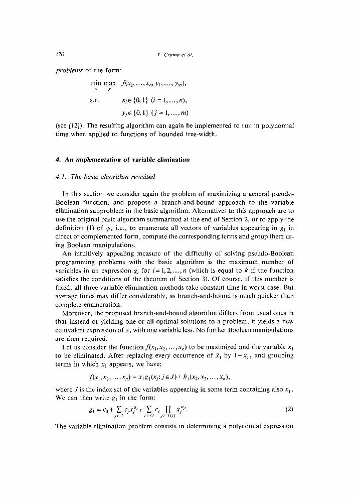
problems of the form:

min max f(xt, . . . ,X,, yl, . . . , Y,), x Y

s.t. XiE{O,l} (i= l,...,n),

,VjE (07 l} (j = 1, ..*,I?Z)

(see [12]). The resulting algorithm can again be implemented to run in polynomial

time when applied to functions of bounded tree-width.

4. An implementation of variable elimination

4. I. The basic algorithm revisited

In this section we consider again the problem of maximizing a general pseudo-

Boolean function, and propose a branch-and-bound approach to the variable

elimination subproblem in the basic algorithm. Alternatives to this approach are to

use the original basic algorithm summarized at the end of Section 2, or to apply the

definition (1) of I,V, i.e., to enumerate all vectors of variables appearing in g, in

direct or complemented form, compute the corresponding terms and group them us-

ing Boolean manipulations.

An intuitively appealing measure of the difficulty of solving pseudo-Boolean

programming problems with the basic algorithm is the maximum number of

variables in an expression gi for i = 1,2, . . . , n (which is equal to k if the function

satisfies the conditions of the theorem of Section 3). Of course, if this number is

fixed, all three variable elimination methods take constant time in worst case. But

average times may differ considerably, as branch-and-bound is much quicker than

complete enumeration.

Moreover, the proposed branch-and-bound algorithm differs from usual ones in

that instead of yielding one or all optimal solutions to a problem, it yields a new

equivalent expression of it, with one variable less. No further Boolean manipulations

are then required.

Let us consider the function f(x,, x2, . . . , x,) to be maximized and the variable x,

to be eliminated. After replacing every occurrence of X1 by 1 -xl, and grouping

terms in which x1 appears, we have:

f(x,,x2, . . . . Xn> =x,g,(xj:jEJ)+hl(X2,Xj, **.,Xn>,

where J is the index set of the variables appearing in some term containing also xl . We can then write g, in the form:

gl = cO + jFJ cjxj*/ + tFQ Ct n x~‘J’- (2)

je T(t)

The variable elimination problem consists in determining a polynomial expression

The basic algorithm for pseudo-Boolean programming revisited 111

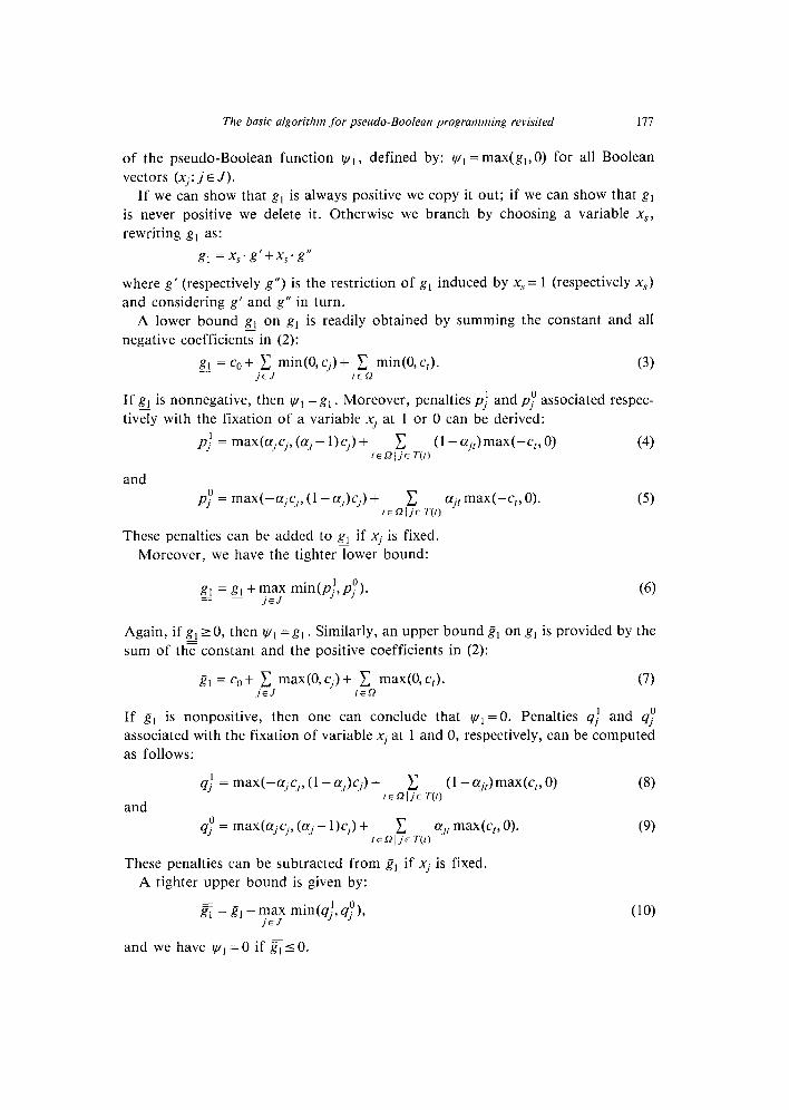
of the pseudo-Boolean function v/~, defined by: v/l = max(g,, 0) for all Boolean

vectors (Xj:jEJ).

If we can show that g, is always positive we copy it out; if we can show that gi

is never positive we delete it. Otherwise we branch by choosing a variable x,,

rewriting g, as:

gl =x,.g’+x,*g”

where g’ (respectively g”) is the restriction of g, induced by x,= 1 (respectively x,)

and considering g’ and g” in turn.

A lower bound gl on g, is readily obtained by summing the constant and all

negative coefficients in (2):

g_! = c~+~~~min(O,c,)+ C min(QcJ. (3) tsS;,

If Q is nonnegative, then tql = g, . Moreover, penalties p,! and p/” associated respec-

tively with the fixation of a variable Xj at 1 or 0 can be derived:

pi’ = maX(CijCj,(tZ-l)Cj)+ C (l-Otjr)maX(-C,, 0) (4) tERljET(!)

and

p: = IIlaX(-CfjCj,(l-CZj)C])+ C tEni./ET(f)

CZj[ max(-c,, 0).

These penalties can be added to g_! if Xj is fixed.

Moreover, we have the tighter lower bound:

g = g_! + mEa; min(pjl,p,O).

(5)

(6)

Again, if g, 2 0, then I,V, = g, . Similarly, an upper bound gi on gl is provided by the

sum of the constant and the positive coefficients in (2):

81 = CO + jzJ max(0, cj) + C maxtO, cI). (7) fER

If g, is nonpositive, then one can conclude that I,U~ =O. Penalties qj and qJ”

associated with the fixation of variable Xj at 1 and 0, respectively, can be computed

as follows:

4; =IllaX(-CfjCj,(l-aj)Cj)+ C (1- ajJmax(c,,O) (8)

and teRIjsT(f)

qJ” = IllaX(oljCj,(olj-l)Cj)+ C (9) fERljET(I)

aj, max(c,, 0).

These penalties can be subtracted from g1 if Xj is fixed.

A tighter upper bound is given by:

E = & - mEa; min(qj’, 4,0), (10)

and we have t,u,=O if c<O.

178 Y. Crama et al.

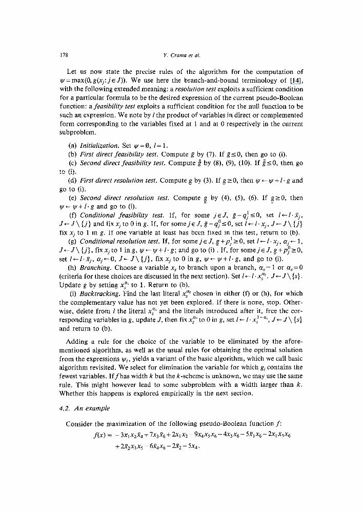
Let us now state the precise rules of the algorithm for the computation of r,u = max(0, g(xj: j E J)). We use here the branch-and-bound terminology of [14], with the following extended meaning: a resolution test exploits a sufficient condition for a particular formula to be the desired expression of the current pseudo-Boolean function: a feasibility test exploits a sufficient condition for the null function to be such an expression. We note by 1 the product of variables in direct or complemented form corresponding to the variables fixed at 1 and at 0 respectively in the current subproblem.

(a) Initialization. Set w =0, I= 1. (b) First direct feasibility test. Compute g by (7). If ~10, then go to (i). (c) Second direct feasibility test. Compute 2 by (B), (9), (10). If H<O, then go

to (i). (d) First direct resolution test. Compute g by (3). If gr 0, then v/ + I+V + 1. g and

go to (i). (e) Second direct resolution test. Compute g by (4), (5), (6). If g>O, then = =

v+-V/+l.g and go to (i). (f) Conditional feasibility test. If, for some jE J, g-q,! ~0, set l+ 1. Xj,

J~J\{j}andfixXjtoOing.If,forsomej~J,~-q~~0,setItI~xj,J~J\(j} fix Xj to 1 in g. If one variable at least has been fixed in this test, return to (b).

(g) Conditional resolution test. If, for some j E J, g +p,? 2 0, set I+ 1. Xj, aj + 1, JtJ\{j},fixXjtoling,Wty/+I.g;andgoto(i).If,forsomejEJ,g+pjO20, set i+f.Zj% Glj+O, J-J\(j), fixXj to 0 in g, ~+t+~/+l*g, and go to (i).

(h) Branching. Choose a variable x, to branch upon a branch, (Y, = 1 or a, = 0 (criteria for these choices are discussed in the next section). Set i+- I * x,“‘. J+ J \ {s} . Update g by setting x: to 1. Return to (b).

(i) Backtracking. Find the last literal x,* chosen in either (f) or (h), for which the complementary value has not yet been explored. If there is none, stop. Other- wise, delete from 1 the literal x,“~ and the literals introduced after it, free the cor- responding variables in g, update J, then fix x,“‘ to 0 in g, set I+ I. xjeas, J+ J \ (s} and return to (b).

Adding a rule for the choice of the variable to be eliminated by the afore- mentioned algorithm, as well as the usual rules for obtaining the optimal solution from the expressions vi, yields a variant of the basic algorithm, which we call basic algorithm revisited. We select for elimination the variable for which gi contains the fewest variables. If f has width k but the k-scheme is unknown, we may use the same rule. This might however lead to some subproblem with a width larger than k. Whether this happens is explored empirically in the next section.

4.2. An example

Consider the maximization of the following pseudo-Boolean function f:

The basic algorithm for pseudo-Boolean programming revisited 179

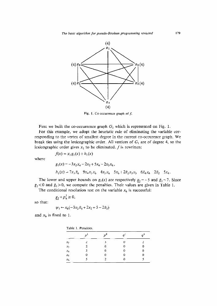
Fig. 1. Co-occurrence graph off.

First we built the co-occurrence graph Gt which is represented on Fig. 1. For this example, we adopt the heuristic rule of eliminating the variable cor-

responding to the vertex of smallest degree in the current co-occurence graph. We break ties using the lexicographic order. All vertices of Gr are of degree 4, so the lexicographic order gives x1 to be eliminated. f is rewritten:

f(x) = Xl g,(x) + h 1 (XI

where

The lower and upper bounds on gt(x) are respectively Q = -5 and g1 = 7. Since gl <O and 8, >O, we compute the penalties. Their values are given in Table 1. -The conditional resolution test on the variable x6 is successful:

g, +p:, 2 0, so that: -

v/l +x6(-3+& + 2x2 + 5 - 2x3)

and x6 is fixed to 1.

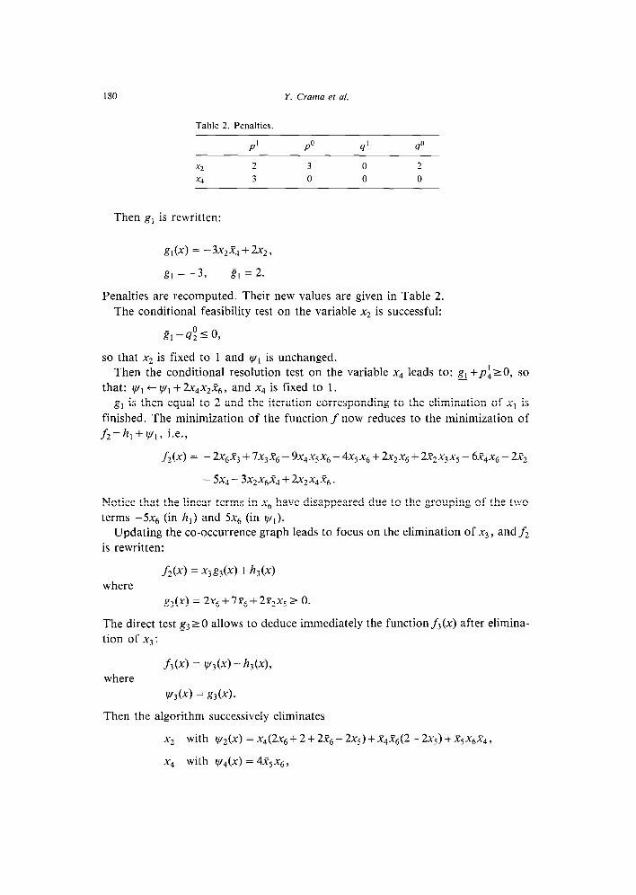
Table 1. Penalties.

P’ PO 4’ 4O

x2 2 3 0 2 x3 2 0 0 0 x4 3 0 0 0 X5 0 0 0 0 X6 5 2 0 5

180 Y. Cruma et al.

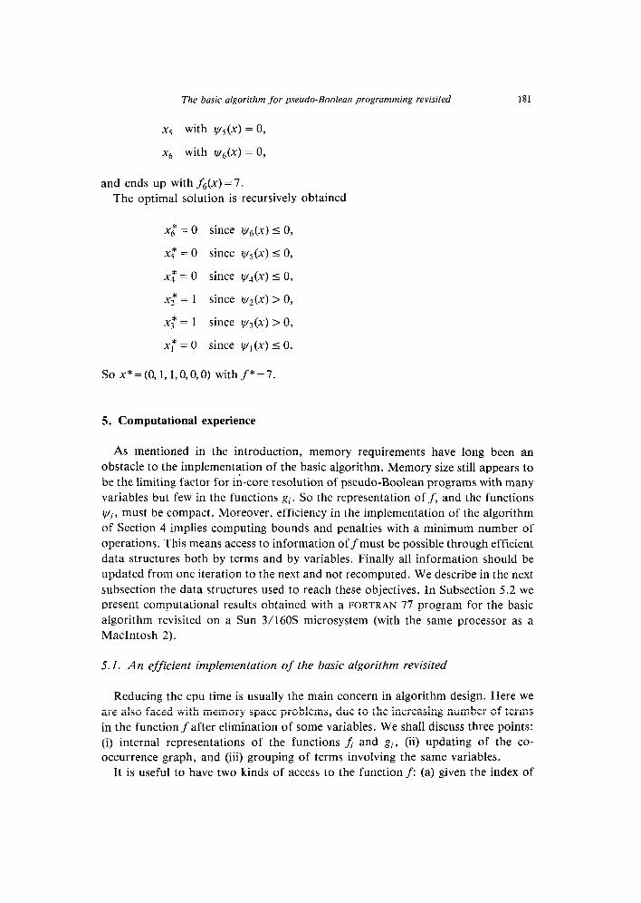
Table 2. Penalties.

P’ PO 4’ 4O

x2 2 3 0 2

x4 3 0 0 0

Then g, is rewritten:

g,(x) = -3x& + 2X,)

gl = -3, 81 = 2.

Penalties are recomputed. Their new values are given in Table 2. The conditional feasibility test on the variable x, is successful:

k&O,

so that x, is fixed to 1 and w1 is unchanged. Then the conditional resolution test on the variable x4 leads to: a +pi>O, so

that: w1 + I+V] +2x4x2X6, and x4 is fixed to 1. g, is then equal to 2 and the iteration corresponding to the elimination of x1 is

finished. The minimization of the function f now reduces to the minimization of fi= hI + wl, i.e.,

fi (X) = - 2x6 .%3 + 7X3 & - 9X4 X5 X6 - 4X5 X6 $2X2 X6 $_ 2x2 X3 X5 - 6.~4 X6 - 2x2

- 5X4-- 3XzX6%!4 + 2X1X4%6.

Notice that the linear terms in x6 have disappeared due to the grouping of the two terInS -5X6 (in hi) and 5x6 (in WI).

Updating the co-occurrence graph leads to focus on the elimination of x3, and fi is rewritten:

where fAx> = X3g3(X) + h,(X)

g,(x)=2x,+7&j+2,Y~x,rO.

The direct test g3 L 0 allows to deduce immediately the function f3(x) after elimina- tion of x3:

where f3(X) = W3(X) + h,(X),

u/3(X) = ‘Lt3(X).

Then the algorithm successively eliminates

x2 with w2(x) = X4(2X,5 + 2 + 2x6 - 2X5) + x4&(2 - 2X5) + x5X$4,

X4 with l,V4(X) = 4n,&j,

The basic algorithm for pseudo-Boolean programming revisited 181

x5 with ws(x) = 0,

xg with I+v~(x) = 0,

and ends up with &(x) = 7.

The optimal solution is recursively obtained

x6* = 0 since we(x) 5 0,

x5* = 0 since ws(x) 5 0,

x4* = 0 since IC/~(X) 5 0,

xz* = 1 since w2(x) > 0,

XT = 1 since w3(x) > 0,

XT = 0 since vi(x) 5 0.

So x* = (0, 1, l,O, 40) with f * = 7.

5. Computational experience

As mentioned in the introduction, memory requirements have long been an

obstacle to the implementation of the basic algorithm. Memory size still appears to

be the limiting factor for in-core resolution of pseudo-Boolean programs with many

variables but few in the functions gi. So the representation off, and the functions

vj, must be compact. Moreover, efficiency in the implementation of the algorithm

of Section 4 implies computing bounds and penalties with a minimum number of

operations. This means access to information offmust be possible through efficient

data structures both by terms and by variables. Finally all information should be

updated from one iteration to the next and not recomputed. We describe in the next

subsection the data structures used to reach these objectives. In Subsection 5.2 we

present computational results obtained with a FORTRAN 77 program for the basic

algorithm revisited on a Sun 3/16OS microsystem (with the same processor as a

Macintosh 2).

5.1. An efficient implementation of the basic algorithm revisited

Reducing the cpu time is usually the main concern in algorithm design. Here we

are also faced with memory space problems, due to the increasing number of terms

in the function f after elimination of some variables. We shall discuss three points:

(i) internal representations of the functions J and g;, (ii) updating of the co-

occurrence graph, and (iii) grouping of terms involving the same variables.

It is useful to have two kinds of access to the function f: (a) given the index of

182 Y. Crama et al.

a term, list all the literals of this term; (b) given a variable xi, list all the terms (and their coefficient) containing Xi or xi. So, we have adopted a double representation off, chaining terms containing each variable and variables in each term. We also chain free spaces. Indeed, at each iteration one variable xi is selected and the derivative of f with respect to this variable is computed. Then the terms of the derivative are removed fromfand thus free some space here and there in the internal representation off. Later some terms corresponding to the function I,Y will be added to f. In order to save memory space, we chain the free spaces obtained when remov- ing the terms of the derivative and insert the terms of v using those spaces first.

The variable to be eliminated corresponds to the vertex of minimal degree in the co-occurrence graph. In case of ties, we use the lexicographic order. So the co-occur- rence graph must be updated at each iteration. This can be done by recomputing the degrees of the vertices corresponding to the variables involved in gi. This is easy, using the second representation off.

In order to save cpu time, the representation of the function gi is not updated each time a variable is fixed in the branch-and-bound procedure, i.e., there is no compression to eliminate terms with a literal fixed at zero, and to reduce terms with a literal fixed at one. Instead, the effect of fixed literals is taken into account during the tests. Due to these fixations, several reduced terms of gi might involve the same product of literals. These lead to obtaining several terms in wi also involving the same product of literals. To avoid increase of the size of v/i due to such terms, they are merged, using an AVL-tree (see e.g. Knuth [16]). Moreover, to avoid having terms with the same product of literals in f, further merging is done between terms of vi and those terms of hi involving only variables of gi. We note hi the sum of these latter terms.

Products of literals are coded by assigning to each of them a number correspon- ding to their position in the list of all products ranked first by increasing length and then by lexicographic order. To keep these numbers sufficiently small, we code only terms all variables of which appear in gi. Complemented variables are coded as variables xl + n. Literals of gi are thus renumbered from 1 to 2k. Each node of the AVL-tree has a value equal to the code number and a label equal to the coefficient of the corresponding term. Terms of hj are first inserted, then those of ‘c/i as soon as they are obtained in the branch-and-bound procedure. The new expression off (after elimination of Xi) is obtained by adding to hi- hj the terms contained in the AVL-tree.

5.2. Experimental results

The basic algorithm revisited has been tested on random pseudo-Boolean func- tions with tree-width at most k, for various fixed values of k. A partial k-tree G = (X, E) on n vertices is first built in the following way [ 191. Initially a set Xi of at most k + 1 vertices is chosen randomly. At iteration r, a subset X, is constructed by: (i) choosing randomly a subset X, among Xi, X2, . . . ,X,_ i , (ii) choosing randomly in

The basic algorithm for pseudo-Boolean programming revisited 183

X, a subset Xi of “attachment vertices”, such that 0 < IX; 1 I k, (iii) adding to X, =

X,’ a random set X: of new vertices (i.e., vertices not belonging to X1 U X, U **- U X,_,) such that IX,~=IX~UX~II~+~, lXJl~1 and IXIUXZU-..UXrl~n. Then a pseudo-Boolean function, the co-occurrence graph of which is a partial

graph of G, is obtained by generating random pseudo-Boolean functions on each

of the sets X,.

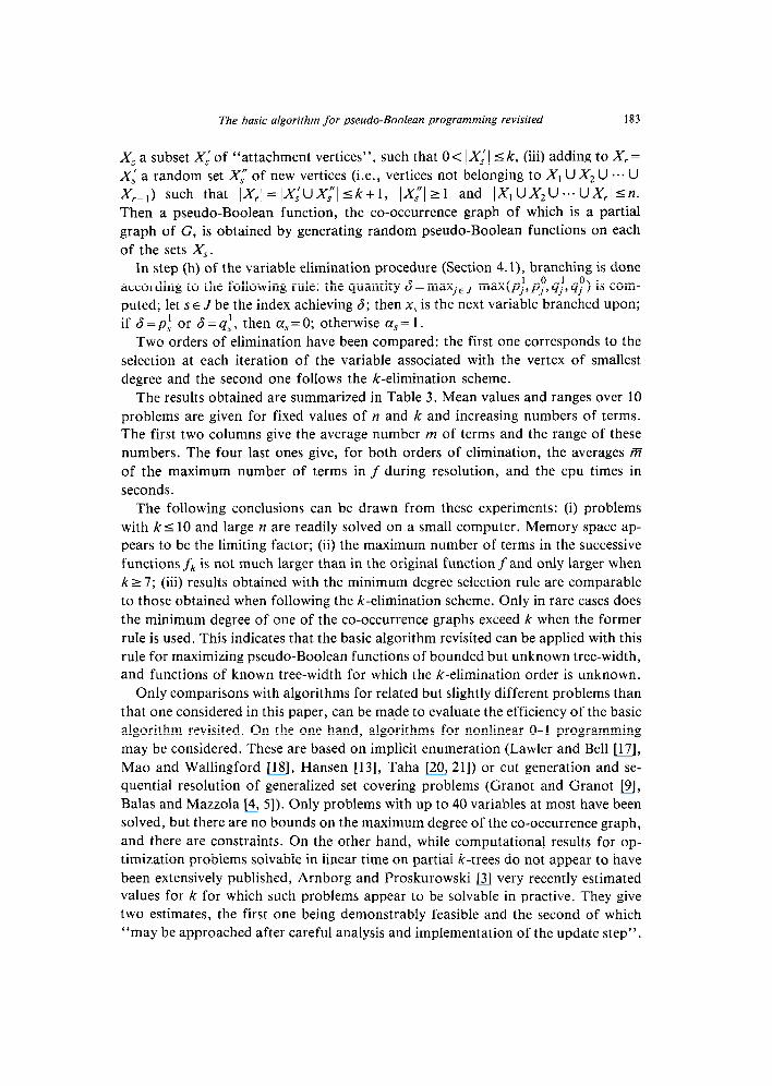
In step (h) of the variable elimination procedure (Section 4.1), branching is done

according to the following rule: the quantity 6 = maxj,, max(p,!,pT, qj, 4;) is com-

puted; let SE J be the index achieving 6; then x, is the next variable branched upon;

if 6 =pi or 6 = qi, then CC, = 0; otherwise a, = 1.

Two orders of elimination have been compared: the first one corresponds to the

selection at each iteration of the variable associated with the vertex of smallest

degree and the second one follows the k-elimination scheme.

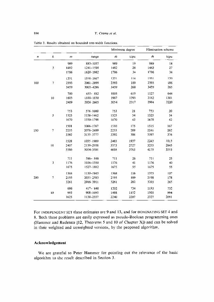
The results obtained are summarized in Table 3. Mean values and ranges over 10

problems are given for fixed values of n and k and increasing numbers of terms.

The first two columns give the average number m of terms and the range of these

numbers. The four last ones give, for both orders of elimination, the averages m

of the maximum number of terms in f during resolution, and the cpu times in

seconds.

The following conclusions can be drawn from these experiments: (i) problems

with ks 10 and large n are readily solved on a small computer. Memory space ap-

pears to be the limiting factor; (ii) the maximum number of terms in the successive

functions fk is not much larger than in the original function f and only larger when

kz7; (iii) results obtained with the minimum degree selection rule are comparable

to those obtained when following the k-elimination scheme. Only in rare cases does

the minimum degree of one of the co-occurrence graphs exceed k when the former

rule is used. This indicates that the basic algorithm revisited can be applied with this

rule for maximizing pseudo-Boolean functions of bounded but unknown tree-width,

and functions of known tree-width for which the k-elimination order is unknown.

Only comparisons with algorithms for related but slightly different problems than

that one considered in this paper, can be made to evaluate the efficiency of the basic

algorithm revisited. On the one hand, algorithms for nonlinear O-l programming

may be considered. These are based on implicit enumeration (Lawler and Bell [17],

Mao and Wallingford [18], Hansen [13], Taha [20, 211) or cut generation and se-

quential resolution of generalized set covering problems (Granot and Granot [9],

Balas and Mazzola [4, 51). Only problems with up to 40 variables at most have been

solved, but there are no bounds on the maximum degree of the co-occurrence graph,

and there are constraints. On the other hand, while computational results for op-

timization problems solvable in linear time on partial k-trees do not appear to have

been extensively published, Arnborg and Proskurowski [3] very recently estimated

values for k for which such problems appear to be solvable in practive. They give

two estimates, the first one being demonstrably feasible and the second of which

“may be approached after careful analysis and implementation of the update step”.

184 Y. Crama et al.

Table 3. Results obtained on bounded tree-width functions.

Minimum degree Elimination scheme

n k m range m tcpu m

3

100 7

10

3

150 7

10

3

200 7

10

989 883-1057 989 19 989 18 1482 1241-1598 1482 28 1482 27

1786 1620-1982 1786 34 1786 34

1351 1016-1667 1351 114 1351 120

2393 2061-2899 2393 189 2393 186

3459 3003-4286 3459 268 3459 265

700 455- 882 1005 619 1127 644

1603 1188-1830 1987 1393 2182 1381

2409 2026-2605 3054 2317 2984 2220

753 576-1000 753 21 753 20

1325 1158-1462 1325 34 1325 34 1670 1550-1798 1670 43 1670 42

1501 1066-1767 1510 175 1515 167

2233 2078-2489 2233 289 224 1 262

3392 3133-3777 3392 386 3397 376

1528 1035-1989 2465 1937 2243 1813

2407 2139-2938 3373 2121 3255 2845

3380 3054-3501 4058 3765 4179 3553

711 586- 848 711 26 711 25 1176 1036-1350 1176 41 1176 40 1675 1527-1882 1675 55 1675 55

1368 1139-1945 1368 116 1375 107 2193 203 l-2583 2193 189 2198 178 3261 2916-3911 3261 282 3265 265

686 417- 840 1202 734 1193 732 993 908-1093 1488 1152 1505 994

1625 1138-2557 2240 2207 2327 2091

- tcpu

For INDEPENDENT SET these estimates are 9 and 13, and for DOMINATING SET 4 and

8. Both these problems are easily expressed as pseudo-Boolean programming ones

(Hammer and Rudeanu [12, Theorems 5 and 10 of Chapter XJ) and can be solved

in their weighted and unweighted versions, by the proposed algorithm.

Acknowledgement

We are grateful to Peter Hammer for pointing out the relevance of the basic

algorithm to the result described in Section 3.

The basic algorithm for pseudo-Boolean programming revisited 185

This research was partially supported by AFOSR grant # 0271 and by the NSF

grant # ECS 8503212 to Rutgers University, by a University of Delaware Research

Foundation grant to the first author and by NSERC grant # GPO036426 and FCAR

grant # 89EQ4144 to the third author.

References

[l] S. Amborg, Efficient algorithms for combinatorial problems on graphs with bounded decom-

posability. A survey, BIT 25 (1985) 2-23.

[2] S. Arnborg, D.G. Corneil and A. Proskurowski, Complexity of finding embeddings in a k-tree,

SIAM .I. Algebraic Discrete Methods 8 (1987) 277-284.

[3] S. Arnborg and A. Proskurowski, Linear time algorithms for NP-hard problems restricted to partial

k-trees, Discrete Appl. Math. 23 (1989) 11-24.

[4] E. Balas and J.B. Mazzola, Nonlinear O-l programming: I. Linearization techniques, Math. Pro-

gramming 30 (1984) 1-21.

[5] E. Balas and J.B. Mazzola, Nonlinear O-l programming: II. Dominance relations and algorithms,

Math. Programming 30 (1984) 22-45.

[6] F. Barahona, A solvable case of quadratic O-l programming, Discrete Appl. Math. 13 (1986) 23-26.

[7] J.A. Bondy and U.S.R. Murty, Graph Theory with Applications (Elsevier, New York, 1976).

]8] G. Georgakopoulos, D. Kavvadias and C.H. Papadimitriou, Probabilistic satisfiability, J. Com-

plexity 4 (1988) 1-11.

[9] D. Granot and F. Granot, Generalized covering relaxation for O-l programs, Oper. Res. 28 (1980)

1442-1449.

[lo] P.L. Hammer (Ivanescu), I. Rosenberg and S. Rudeanu, On the determination of the minima of

pseudo-Boolean functions, Stud. Cert. Mat. 14 (1963) 359-364 (in Romanian).

[l l] P.L. Hammer (lvanescu), I. Rosenberg and S. Rudeanu, Application of discrete linear program-

ming to the minimization of Boolean functions, Rev. Math. Pures Appl. 8 (1963) 459-475 (in

Russian).

[12] P.L. Hammer and S. Rudeanu, Boolean Methods in Operations Research and Related Areas

(Springer, New York, 1968).

[13] P. Hansen, Programmes mathematiques en variables O-l, These d’aggregation, Universite Libre de

Bruxelles, Bruxelles (1974).

[14] P. Hansen, Les procedures d’optimisation et d’exploitation par separation et evaluation, in: B. Roy,

ed., Combinatorial Programming (Reidel, Dordrecht, 1975) 19-65.

[15] P. Hansen and B. Simeone, Unimodular functions, Discrete Appl. Math. 14 (1986) 269-281.

[16] D.E. Knuth, The Art of Computer Programming, Vol. 3: Sorting and Searching (Addison-Wesley,

Reading, MA, 2nd ed., 1975).

[17] E.L. Lawler and M.D. Bell, A method for solving discrete optimization problems, Oper. Res. 14

(1966) 1098-1112.

[18] J.C.T. Mao and B.A. Wallingford, An extension of Lawler and Bell’s method of discrete optimiza-

tion with examples from capital budgeting, Management Sci. 15 (1968) 51-60.

]19] N. Robertson and P.D. Seymour, Graph minors: II. Algorithmic aspect of tree-width, J.

Algorithms 7 (1986) 309-322.

[20] H. Taha, A Balasian-based algorithm for zero-one polynomial programming, Management Sci. 18B

(1972) 328-343.

[21] H. Taha, Further improvements in the polynomial zero-one algorithm, Management Sci. 19 (1972)

226-227.