THE FEASIBILITY OF ASEAN+6 SINGLE CURRENCY: A VECTOR ERROR CORRECTION MODEL

ASEAN Journal of Economics, Management and Accounting 1 (1): 23-47 (June 2013) ISSN 2338-9710

THE FEASIBILITY OF ASEAN+6 SINGLE CURRENCY: A VECTOR ERROR CORRECTION MODEL Noer Azam Achsani

Department of Economics and Graduate School of Management and Business, Bogor Agricultural University, Indonesia

Hari Wijayanto

Department of Statistics, Faculty of Mathematics and Natural Science, Bogor Agricultural University, Indonesia

Erfira Sefitri

Department of Statistics, Faculty of Mathematics and Natural Science, Bogor Agricultural University, Indonesia

Dina Lianita Sari Brighten Institute, Jl. Merak No 14 Bogor

Corresponding author:

[Submitted June 2013, Accepted September 2013]

Abstract. This paper explore the possibility of the establishment of a single currency among ASEAN countries and six other counties, namely China, South Korea, Japan, Australia, New Zealand and India. We simulated the single currency by using weighted average and principal component analysis methods. Those methods are applied to compare the stability of the single currency. Furthermore, this paper will also identify the possible impact of the exchange rate shocks to the member countries by analyzing the impulse response function. The results showed the single currency established by applying weighted average method is more stable than those of principal component analysis. The weights used in this method are the exchange rate volatilities of each ASEAN+6 countries. Moreover, impulse response function showed that the single currency will give much benefit to member countries, especially to Indonesia, Malaysia, Singapore, Philippines, Thailand, Vietnam, and China.

Keywords: ASEAN+6, single currency, weighted average, principal component analysis, error correction model

JEL Codes: E32, F02, F15, F31

Introduction

Economic crisis, hitting Asia in 1997, has triggered the ASEAN countries to

integrate their economy. According to Kurniati (2007), the economic integration in one

region is established by considering not only the geographical and historical similarity,

but also economic relationship among countries in that region. The phenomenal

process was the establishment of European Union (EU), which integrated Europe

economy in the single market, with the single currency, named EURO. The single

market involves the free circulation of goods, capital, people and services within the EU,

and the customs union involves the application of a common external tariff on all goods

entering the market. This efficiency has boosted the economy of EU countries,

moreover EU can compete with the dominance of US economy.

The success story of the EU in establishing a single market in 1999 have motivated

ASEAN region to create the single market. During ASEAN Summit in Bali October 2003,

all ASEAN members agreed to establish a so-called “ASEAN Economic Community

24

(AEC)” as the realization and end-goal of economic integration as outlined in the ASEAN

Vision 2020. It rearticulates its aims to create a stable, prosperous and highly

competitive ASEAN economic region in which there is a free flow of goods, services,

investment and a freer flow of capital, equitable economic development and reduced

poverty and socio-economic disparities. The AEC plans to establish ASEAN as single

market and production base, turning the diversity that characterizes the region into

opportunities for business complementation making the ASEAN a more dynamic and

stronger segment of the global supply chain.

Furthermore, the AEC involves not only the ASEAN countries, but also six other

nations (China, India, Japan, South Korea, Australia and New Zealand), which is known

as the ASEAN+6 group. They agreed to accelerate economic growth in East Asian

countries, promote cooperation in energy, foods, and other fields vital to economic

activities. The AEC establishment will end in the creation of a regional currency unit

that had often been referred to as the Asian Currency Unit (ACU).

Some studies concerning the single currency establishment have been carried out.

Study of Bayoumi and Mauro (2008) resulted that ASEAN condition has not yet fulfilled

the single currency criteria. Moreover, Partisiwi (2010) analyzed the possibility of

currency integration among ASEAN+3 countries by using Optimum Currency Areas

(OCA) criteria. The result showed that Singapore Dollar was the most stable currency in

the region during the period of analysis. However, this paper will involve a wider

region, which are ASEAN+6 countries.

Drawing on the experience with the European Currency Unit (ECU) in the

European Monetary System (EMS), proponents of an Asian currency basket have

argued that the basket could play two key roles in the context of ASEAN+6. First, the

basket could provide a framework for specifying exchange rate objectives as part of any

formal effort to coordinate exchange rate policies. Such an approach would build, in

particular, on the role the ECU notionally played in specifying exchange rate targets and

divergence indicators in the exchange rate mechanism of the European Monetary

System (EMS). Second, irrespective of whether there is formal agreement on exchange

rate polices, the creation of an official currency basket could usefully catalyze the

private sector into denominating financial assets in the basket along the lines the

official ECU played in European Monetary System (EMS). Within the region, this has

become known (somewhat misleadingly) as the parallel currency proposal

(Eichengreen (2006)) and as leading (potentially) to the emergence of the ACU as a

parallel currency alongside national currencies.

The objective of this paper is to get a single currency for ASEAN+6 countries (ACU)

by using weighted average and principal component analysis methods. Those methods

are applied to compare the stability of single currency. To this end, this paper will also

try to identify the impact of ACU and exchange rate shocks of the countries by analyzing

the impulse response function.

The rest of the paper will be organized as follows: Section 2 will explain the data

and research methodology, followed by a discussion on section 3. Summary of the

results and the policy implications will be provided in section 4.

Research Method

We used the macroeconomic data covering the period December 1999–December

2009, from ASEAN countries (i.e. Indonesia, Malaysia, Singapore, Thailand, Philippines,

Vietnam, Cambodia, and Laos) plus six other countries of China, India, Japan, South

Korea, Australia and New Zealand. The macroeconomic variables applied are exchange

rate, GDP, and inflation rate. The data are collected from World Economic Outlook Database April 2009 and the CEIC Database.

ASEAN Journal of Economics, Management and Accounting

25

The stages of data analysis in this paper are as follows:

1. Analyze descriptively the exchange rate among the ASEAN+6 countries.

2. Find the ACU by using weighted average method, where the weight applied is

volatility of the exchange rate, GDP, and inflation rate.

3. Find the ACU by using principal component analysis method.

4. Compare the ACU stability obtained in step 2 and 3.

5. Apply VAR or VECM methods to analyze the feasibility of each country joining in

ACU. The full steps are given in Appendix 1, or briefly, as follows:

� Transform each variable to its logarithm.

� Check the data stationary by using ADF test. If it is not, then take differencing.

� Determine the optimal lag.

� Examine the cointegration by using Johansen test.

� Establish the VAR or VECM model

� Analyze the IRF and FEVD

Those steps above are carried out using software Microsoft Excel 2007, Eviews 5.1

and Minitab 14.

Weighted Average

The weighted average is a method, where instead of each of the data points

contributing to the final average, in such a way that the total weight is .

Therefore, the weighted average is defined as:

where

= linear combination of variables and their weights

= the i-th weight

= the i-th variable

The weights used in this paper are as follows:

1. Volatility is the data fluctuation in the certain period, or statistically, known as

standard deviation. In this paper, we use invers of the exchange rate volatility of

each country. So, the exchange rate with a great volatility will be weighted lower

than that which has a small volatility.

2. Gross Domestic Product (GDP) is a measure of a country's overall economic output.

It is the market value of all final goods and services made within the borders of a

country in a certain period. GDP is a sum of consumption (C), investment (I),

government spending (G) and net exports (X), or mathematically, defined as:

In this paper, we use nominal GDP.

3. Inflation is a rise in the general level of prices of goods and services in an economy

over a period of time. A chief measure of price inflation is the inflation rate, the

annualized percentage change in a general price index (normally the Consumer

Price Index) over time. We formulate the inflation rate as follow:

26

where

= inflation rate at the t-th period

= consumer price index at the t-th period

In this paper, we use invers of the inflation rate.

Principal Component Analysis

The principal component analysis (PCA) is a method that reduces data

dimensionality by performing a covariance analysis between factors. The PCA involves

a mathematical procedure that transforms a number of possibly correlated variables

into a smaller number of uncorrelated variables called principal components. PCA was

invented in early 1900 by Karl Pearson. Hotelling (1933) developed the procedure

applying in the random vectors. Then, Rao (1964) used the PCA procedure in various

applied research.

Given a set of points in Euclidean space, the first principal component (the eigen

vector with the largest eigen value) corresponds to a line that passes through the mean

and minimizes sum squared error with those points. The second principal component

corresponds to the same concept after all correlation with the first principal component

has been subtracted out from the points. Each eigen value indicates the portion of the

variance that is correlated with each eigen vector. Thus, the sum of all the eigen values

is equal to the sum squared distance of the points with their mean divided by the

number of dimensions. PCA essentially rotates the set of points around their mean in

order to align with the first few principal components. This moves as much of the

variance as possible (using a linear transformation) into the first few dimensions. The

values in the remaining dimensions, therefore, tend to be highly correlated and may be

dropped with minimal loss of information. PCA is often used in this manner for

dimensionality reduction. PCA has the distinction of being the optimal linear

transformation for keeping the subspace that has largest variance.

In practice, a random sample of n individuals are obtained on p variables. The data

for a PCA consists of an (n × p) data matrix Y and an (n × q) data matrix X of q

covariates. To perform a PCA, one employs the unbiased estimator S for � or the

sample correlation matrix R. Selecting between S and R depends on whether the

measurements are commensurate. If the scales of measurements are commensurate,

one should analyze S, otherwise R is used. Never use R if the scales are commensurate

since by forcing all variables to have equal sample variance one may not be able to

locate those components that maximize the sample dispersion.

Replacing � with S, one solves | | 0�� S I to obtain eigen values and eigen

vectors usually represented as j� and jp . Thus, the sample eigen vectors become P

and the sample eigen values become diag[ ]j�� . The formula for the standardized

principal components for all n individuals is

Where dY is the matrix of deviation scores after subtracting the sample means and Q

are the sample covariance.


27

Vector Auto Regression (VAR)

The vector auto regression (VAR) model is one of the most successful, flexible, and

easy to use models for the analysis of multivariate time series. It is a natural extension

of the univariate autoregressive model to dynamic multivariate time series. The VAR

model has proven to be especially useful for describing the dynamic behavior of

economic and financial time series and for forecasting. It often provides superior

forecasts to those from univariate time series models and elaborate theory-based

simultaneous equations models. Forecasts from VAR models are quite flexible because

they can be made conditional on the potential future paths of specified variables in the

model.

In addition to data description and forecasting, the VAR model is also used for

structural inference and policy analysis. In structural analysis, certain assumptions

about the causal structure of the data under investigation are imposed, and the

resulting causal impacts of unexpected shocks or innovations to specified variables on

the variables in the model are summarized. These causal impacts are usually

summarized with impulse response functions and forecast error variance

decompositions.

VAR models in economics were made popular by Sims (1980). The definitive

technical reference for VAR models is Lutkepohl (1991), and updated surveys of VAR

techniques are given in Watson (1994) and Lutkepohl (1999) and Waggoner and Zha

(1999). Applications of VAR models to financial data are given in Hamilton (1994),

Campbell, Lo and MacKinlay (1997), Cuthbertson (1996), Mills (1999) and Tsay (2001).

For a set of n time series variables )'...,,( ,21 ntttt yyyy � , a VAR model of order p

(VAR(p)) can be written as:

tptpttt uyAyAyAy �� ...2211

where the iA ’s are (nxn) coefficient matrices and )',...,,( 21 ntttt uuuu � is an unobservable

i.i.d. zero mean error term.

Impulse Response Functions (IRF)

Impulse response function is used when we want to trace out the time path of the

effect of structural shocks on the dependent variables of the model. More generally, an

impulse response refers to the reaction of any dynamic system in response to some

external change. In both cases, the impulse response describes the reaction of the

system as a function of time (or possibly as a function of some other independent

variable that parameterizes the dynamic behavior of the system).

Forecast Error Variance Decomposition (FEVD)

Forecast error variance decomposition indicates the amount of information each

variable contributes to the other variables in a VAR model. Variance decomposition

determines how much of the forecast error variance of each of the variable can be

explained by exogenous shocks to the other variables. In other word, It tells how much

of a change in a variable is due to its own shock and how much due to shocks to other

variables. In the short run, most of the variation is due to own shock. But as the lagged

variables’ effect starts kicking in, the percentage of the effect of other shocks increases

over time.

28

Empirical Results

Descriptive Analysis of Exchange Rate of ASEAN+6 Countries Currencies

The exchange rate movement is different among ASEAN+6 countries, clearly

presented in Appendix 2. In general, the exchange rate of Malaysia, Singapore, Thailand,

Japan, China, Australia and New Zealand appreciated to the US dollar in the period

2000-2008. Furthermore, the volatility of Indonesian exchange rate was the highest

among other countries, i.e. 0.042. Whereas, exchange rate of China was eleven times

more stable than Indonesia, i.e. 0.0038.

As seen in Appendix 3, the exchange rate tended to be unstable among countries in

period 2000-2001. The economic crisis in 1997 still affected the ASEAN+6 countries, so

that the currencies were very volatile. Nevertheless, in 2002, the countries had

overcome that global financial crisis, therefore the exchange rate started to be stable in

this period. The graphs in Appendix 3 also indicate that Malaysia, Vietnam, Cambodia,

and China had succeeded in holding the exchange rate relative stable over the years.

Before establishing a single currency, we need to know the correlation of the

exchange rate every ASEAN+6 member. It is completely provided in Appendix 4. The

Pearson test result the significant correlation among the countries’ exchange rates,

which is summarized in Table 1.

Table 1 Correlation of the Exchange Rates of ASEAN+6 Countries (α = 5%)

Indo Cam, Chi, Kor, Ind, Aus, Nz

Mal Sing, Phi, Tha, Vie, Cam, Lao, Jap, Chi, Kor, Ind, Aus, Nz

Sing Mal, Phi, Tha, Vie, Cam, Lao, Jap, Chi, Kor, Ind, Aus, Nz

Phi Mal, Sing, Tha, Cam, Lao, Chi, Kor, Ind

Tha Mal, Sing, Phi, Vie, Cam, Lao, Jap, Chi, Kor, Ind, Aus, Nz

Vie Mal, Sing, Tha, Cam, Lao, Jap, Chi, Kor, Ind, Aus, Nz

Cam Indo, Mal, Sing, Phi, Tha, Vie, Lao, Chi, Kor, Ind, Aus, Nz

Lao Mal, Sing, Phi, Tha, Vie, Cam, Jap, Chi, Nz

Jap Mal, Sing, Tha, Vie, Lao, Chi, Kor, Ind, Aus, Nz

Chi Indo, Mal, Sing, Phi, Tha, Vie, Cam, Lao, Jap, Kor, Ind, Aus, Nz

Kor Indo, Mal, Sing, Phi, Tha, Vie, Cam, Jap, Chi, Ind, Aus, Nz

Ind Indo, Mal, Sing, Phi, Tha, Vie, Cam, Jap, Chi, Kor, Aus, Nz

Aus Indo, Mal, Sing, Tha, Vie, Cam, Jap, Chi, Kor, Ind, Nz

Nz Indo, Mal, Sing, Tha, Vie, Cam, Lao, Jap, Chi, Kor, Ind, Aus,

Based on the Table 1, the Indonesian exchange rate has the fewest correlations

with other countries. However, China has correlation with all the countries. The

correlations between Malaysia, Singapore, and Thailand are positively strong enough. It

means that the exchange rates among those three countries tend to be similar.

Furthermore, the strong and positive correlations were occurred not only between

China and Malaysia, Singapore, Thailand, but also between Australia and Singapore,

Thailand, Korea, New Zealand.

The ASEAN+6 Single Currency Establishment Using Weighted Average Method

Each ASEAN+6 exchange rate has different volatility. We use the inverse of that

volatility to obtain the weight of each country, so the country that has a great volatility

will be given by a small weight. Result of the weights can be seen in Table 2.

Based on Table 2, the exchange rate volatility of Indonesia, Vietnam, Cambodia,

Laos, Japan, Australia, and New Zealand tends to decrease period-by-period, therefore

their weights become larger. It is different for Singapore, Philippines, Thailand, Korea,

and India, which tend to increase all over periods.


29

The ACU is also can be established from linear combination of the exchange rate,

weighted by using GDP and inflation rate. The results of those weights are given in

Table 3 and Table 4, respectively.

Table 2 The ACU Weights Based on Exchange Rate Volatility (%)

Country Period

2000-2004 2004-2008 2000-2008 Indo 0.001 0.002 0.001

Mal* - 5.296 5.296

Sing 20.980 9.313 7.911

Phi 0.229 0.199 0.216

Tha 0.467 0.327 0.272

Vie 0.002 0.004 0.002

Cam 0.016 0.019 0.011

Lao 0.001 0.001 0.001

Jap 0.126 0.149 0.128

Chi* - 1.977 2.145

Kor 0.014 0.009 0.007

Ind 0.638 0.419 0.392

Aus 4.435 8.919 3.572

Nz 2.865 8.383 2.565

Stdev 9.544 10.280 7.701 Note:

(*) calculated in July 2005-Desember 2008, because of the exchange rate system

change.

Table 3 The ACU Weights Based on GDP (%)

Country Period

2000-2004 2004-2008 2000-2008 Indo 2.490 3.267 2.967

Mal 1.283 1.462 1.395

Sing 1.154 1.268 1.227

Phi 0.959 1.087 1.046

Tha 1.644 1.878 1.788

Vie 0.452 0.565 0.522

Cam 0.054 0.068 0.063

Lao 0.025 0.032 0.029

Jap 52.909 40.310 45.241

Chi 18.549 25.783 23.012

Kor 7.326 7.970 7.708

Ind 6.566 8.190 7.558

Aus 5.747 7.111 6.517

Nz 0.841 1.008 0.927

Stdev 25.302 31.255 28.919

Table 3 explains that GDP contribution of each ASEAN+6 member tend to increase,

and relatively similar between period 2000-2004 and period 2004-2008. Japan has a

greatest contribution among ASEAN+6 countries, but it tends to decrease from 52.9%

(period 2000-2004) to 40.3% (period 2004-2008), otherwise Vietnam, Cambodia, Laos,

and New Zealand have the smaller contribution among those countries. The ACU

establishment using the GDP of each country gives the volatility 28.9 percent.

30

Table 4 The ACU Weights Based on Inflation Rate (%)

Country Period

2000-2004 2004-2008 2000-2008 Indo 1.492 1.905 1.580

Mal 7.047 6.259 6.406

Sing 13.828 13.763 14.236

Phi 2.376 2.907 2.589

Tha 7.418 4.494 6.363

Vie 8.894 1.707 6.485

Cam 14.416 2.724 10.422

Lao 0.847 2.312 1.413

Jap 17.997 38.805 24.977

Chi 12.539 5.885 10.507

Kor 3.213 5.341 4.027

Ind 2.539 2.959 2.589

Aus 3.131 5.487 3.837

Nz 4.263 5.452 4.570

Stdev 75.216 35.794 59.788

Table 4 indicates the weights based on the inflation rate. In the same way as GDP

contribution, we use inverse of the inflation rate. Therefore, country with high inflation,

like Laos, will be given a small weight. Otherwise, we give the larger weight for Japan

because of its low inflation. In the period 2000-2008, the ACU establishment using the

inflation rate of each country gives the volatility 59.8 percent. Table 5 gives the ACU

weights based on the GDP and the inflation rate, where each variable is weighted as 50

percent.

Table 5 The ACU Weights Based on GDP and Inflation Rate (%)

Country Period

2000-2004 2004-2008 2000-2008 Indo 1.991 2.586 2.273

Mal 4.165 3.861 3.900

Sing 7.491 7.516 7.731

Phi 1.668 1.997 1.818

Tha 4.531 3.186 4.075

Vie 4.673 1.136 3.503

Cam 7.235 1.396 5.243

Lao 0.436 1.172 0.721

Jap 35.453 39.557 35.109

Chi 15.544 15.834 16.759

Kor 5.270 6.655 5.867

Ind 4.553 5.574 5.074

Aus 4.439 6.299 5.177

Nz 2.552 3.230 2.749

Stdev 42.302 30.140 37.280

In Table 5, we composite the variable GDP and variable inflation rate, in order to

obtain new weights. Japan is given a larger weight than other countries, because it has

large GDP and low inflation. But, we give a smaller weight for Laos, i.e. 0.72 percent in

the period 2000-2008. The volatility of this single currency is 37.28 percent.


31

The ASEAN+6 Single Currency Establishment Using PCA

The single currency for ASEAN+6 countries was also established by using principal

component analysis. Applying this method, we had principal components (PC) derived

from linear combinations of each ASEAN+6 exchange rate, so that the information

in the PC was composite of all exchange rates with certain weights. For every

principal component, we obtain its eigen value and variance. It is clearly given in Table

6. In this paper, we choose a PC with the largest variance; therefore, information of each

exchange rate will be explained maximum.

Table 6 The Characteristic Root and Variance of the Principal Components

Eigen Value Variance (%)

Variance Cumulative (%)

PC1 7.559 53.991 53.991

PC2 2.942 21.015 75.006

PC3 1.497 10.691 85.697

PC4 0.931 6.649 92.346

PC5 0.509 3.636 95.982

PC6 0.277 1.979 97.960

PC7 0.089 0.639 98.599

PC8 0.067 0.478 99.077

PC9 0.055 0.391 99.467

PC10 0.028 0.199 99.667

PC11 0.019 0.134 99.800

PC12 0.014 0.102 99.902

PC13 0.008 0.056 99.958

PC14 0.006 0.042 100.000

Table 7 The weights of ACU Using Principal Component Analysis Method

Negara Eigen Vector of PC1

Indo -0.02045

Mal -0.31811

Sing -0.35173

Phi -0.15808

Tha -0.34444

Vie 0.234603

Cam 0.267421

Lao -0.02228

Jap -0.16855

Chi -0.28268

Kor -0.29663

Ind -0.29518

Aus -0.34376

Nz -0.32001

Standard Deviation 192.446

From the Table 6, we should use the first PC (PC1), which has eigen value 7.56 and

the largest variance among others, i.e. 53.99 percent. In the other words, the PC1 can

explain 53.99 percent of the exchange rate variety every ASEAN+6 countries. Using that

eigen value, we also can obtain the eigen vector consist of the weights of ACU, which is

given in Table 7. The single currency established has volatility 192.45.

32

Comparison between Weighted Average Method and PCA Method

The single currency establishment using weighted average and principal

component analysis methods indicates different characteristics. We can check the

stability of the ACU through the volatility the currency all over years. Clearly, it is

described in Figure 1.

Based on the Figure 1, the ACU established using weighted average method is

relatively stable. However, the principal component analysis results the high unstable

ACU with standard deviation 192.45. The minimum volatility of ACU is established

using weighted average method, where the weights are the exchange rate of each

ASEAN+6 country. Therefore, we can apply this method to establish the stable

ASEAN+6 currency. Furthermore, we will use this result in analyzing the response of

each country to the ACU establishment.

Figure 1 The Trend of ACU Using Weighted average Method and Principal Component

Analysis Method

Response of ASEAN+6 Countries to the ACU Establishment

In this part, we will identify the feasibility of each ASEAN+6 country in changing its

currency to the ACU. To solve this problem, we can apply a VAR or VECM model. The

variables used in this model are the exchange rate of each ASEAN+6 country and the

stable single currency established by using weighted average method. Besides that, we

will also identify the response of each country to the shock of the greatest currencies in

the world, i.e. US Dollar and Euro.

Before applying VAR or VECM estimation, we should carry out some tests in order

to obtain an appropriate model. The tests include stationary test, optimal lag

determination, cointegration test. We will briefly explain those tests below.

Data Stationarity Test

The first step is checking the stationarity all the variables using Augmented Dickey-

Fuller (ADF) test. The test indicates that all the variables are stationary in their first

difference, except to Indonesia exchange rate, which is stationary in level. Result of the

stationary test can be seen in Table 8.


33

Table 8 Unit Root Test Using Augmented Dickey-Fuller (ADF)

Variable Level First difference Indo -3.861*

Mal 0.376 -3.236* Sing -0.495 -7.918* Phi -2.207 -8.949* Tha -0.928 -6.893* Vie -1.865 -11.329* Kam -2.294 -10.180* Lao -2.222 -7.908* Jep -0.479 -8.758* Chi 2.413 -3.578* Kor -1.197 -8.382* Ind -1.972 -6.383* Aus -1.373 -7.029* Nz -1.301 -7.024* ACU -1.703 -6.875* USD -1.209 -7.023* Euro -0.806 -7.121*

Note: *) the variable is stationary at α = 5%

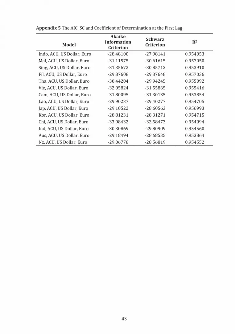
Optimal Lag Determination

The second step is determining the optimal lag used in the estimation. However,

we need to examine the model stability, so that the maximum lag will be obtained. In

our paper, the model is stable in the first lag, therefore we do need check the AIC, SC,

and adjusted R2. The test result is given in Appendix 5.

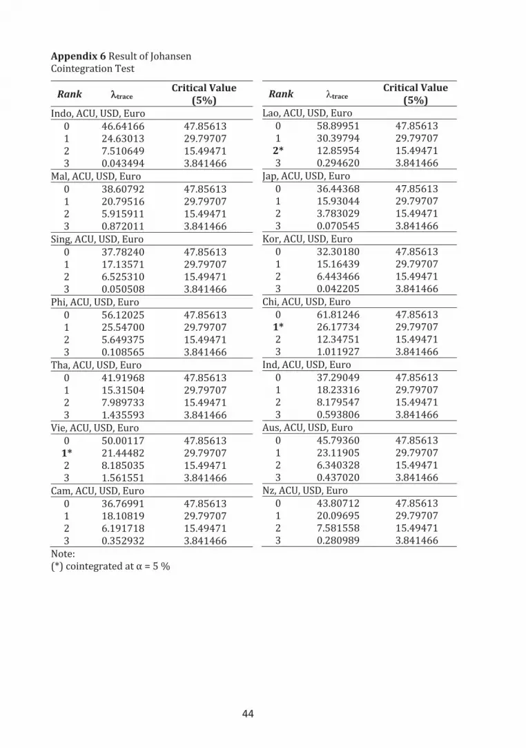
Cointegration Test

The cointegration test is applied because there are variables in the model that are

not stationary in level, but stationary in first difference. It is possibly that there are

cointegration among variables, or in other words, there are long run relationship

among variables. We use Johansen cointegration test, the result can be seen in

Appendix 6.

Result of the cointegration test indicates that there are cointegration between

variable Vietnam, Laos, China and ACU, USD, and Euro. Therefore, we use VECM model

for those three countries, whereas we use first-order VAR model for other countries.

Table 9 summarizes models used in this paper.

Impulse Response Functions (IRF) of the ASEAN+6 Countries

Impulse responses trace out the response of current and future values of each of

the variables to a one-unit increase in the current value of one of the standard

deviation. It is a one-period shock, which reverts to zero immediately. The figure of

impulse responses is presented in Figure 2.

Based on the Figure 2, shocks of ACU, USD, and Euro have different impacts to the

ASEAN+6 countries. The ACU shock tends to be stable in the next three years applied in

Indonesia, Malaysia, Singapore, Thailand, Vietnam, Cambodia, Laos, and China.

However, the ACU shock in the other countries, i.e. Japan, India, Australia, and New

Zealand, tend to be unstable. In the Philippines and Korea, shock of the ACU has a small

effect, and not in their equilibrium in next three years. The impact of the USD and Euro

34

currencies is clearly seen in Philippines, Japan, Korea, India, Australia, and New

Zealand. Consequently, the ACU has not given more benefits to these countries.

Table 9 Models Established in This Paper

Variable Model

Indo, ACU, USD, Euro VAR (1)-1st difference Mal, ACU, USD, Euro VAR (1)-1st difference

Sing, ACU, USD, Euro VAR (1)-1st difference

Phi, ACU, USD, Euro VAR (1)-1st difference

Tha, ACU, USD, Euro VAR (1)-1st difference

Vie, ACU, USD, Euro VECM (1), rank 1

Cam, ACU, USD, Euro VAR (1)-1st difference

Lao, ACU, USD, Euro VECM (1), rank 2

Jap, ACU, USD, Euro VAR (1)-1st difference

Kor, ACU, USD, Euro VAR (1)-1st difference

Chi, ACU, USD, Euro VECM (1), rank 1

Ind, ACU, USD, Euro VAR (1)-1st difference

Aus, ACU, USD, Euro VAR (1)-1st difference

Nz, ACU, USD, Euro VAR (1)-1st difference

Forecast Error Variance Decomposition (FEVD) of the ASEAN+6 Countries

Forecast error variance decomposition determines how much of the forecast error

variance of each of the ASEAN+6 exchange rate can be explained by exogenous shocks,

i.e. ACU, US Dollar, and Euro, to the other variables in the certain period.

Result of FEVD of each country is presented in Appendix 7.

In the long run, the variance of the exchange rate most of the ASEAN+6 countries,

i.e. Indonesia, Malaysia, Singapore, Thailand, Vietnam, Laos, Japan, India, and New

Zealand, are mainly explained by US Dollar variance. It implies that those countries are

greatly influenced by US Dollar. However, Euro explains the variance of exchange rates

in Philippines, Cambodia, and Australia. The variance of exchange rate in China is

dominated by itself in the long run. It indicates that China currency is greatly influenced

by its internal factor in the next three years.

Conclusion

The volatilities of exchange rate among ASEAN+6 countries are highly varied. The

highest volatility is experienced by Indonesia, i.e. 0.042, whereas China has a minimum

volatility, i.e. 0.0038. Based on those exchange rates, we establish a single currency,

formally called as Asian Currency Unit (ACU). The ACU is resulted by using two

methods, i.e. weighted average method and principal component analysis method. By

comparing the standard deviation, the ACU established by applying weighted average

method is more stable than another method. The weights used in this method are the

exchange rate volatilities of each ASEAN+6 country.

Based on the impulse response function, we can know the response of each

country if there are shocks of the ACU, US Dollar, and Euro. The result indicates that

Japan, India, Australia, and New Zealand will need a longer time to establish the single

currency. However, we predict that the ACU establishment in the short future will give

much benefit in the other countries, i.e. Indonesia, Malaysia, Singapore, Philippines,

Thailand, Vietnam, and China.


35

Figure 2 The IRF of Each Country to the to ACU, US Dollar and Euro

-.3

-.2

-.1

.0

.1

.2

.3

5 10 15 20 25 30 35

ACU USDOLLAR EURO

Response of JEPANG to CholeskyOne S.D. Innovations

-.3

-.2

-.1

.0

.1

.2

.3

5 10 15 20 25 30 35

ACU USDOLLAR EURO

Response of New Zealand to CholeskyOne S.D. Innovations

-.3

-.2

-.1

.0

.1

.2

.3

5 10 15 20 25 30 35

ACU USDOLLAR EURO

Response of INDIA to CholeskyOne S.D. Innovations

-.3

-.2

-.1

.0

.1

.2

.3

5 10 15 20 25 30 35

ACU USDOLLAR EURO

Response of AUSTRALIA to CholeskyOne S.D. Innovations

-.3

-.2

-.1

.0

.1

.2

.3

5 10 15 20 25 30 35

ACU USDOLLAR EURO

Response of FILIPINA to CholeskyOne S.D. Innovations

-.3

-.2

-.1

.0

.1

.2

.3

5 10 15 20 25 30 35

ACU USDOLLAR EURO

Response of MALAYSIA to CholeskyOne S.D. Innovations

-.3

-.2

-.1

.0

.1

.2

.3

5 10 15 20 25 30 35

ACU USDOLLAR EURO

Response of LAOS to CholeskyOne S.D. Innovations

-.3

-.2

-.1

.0

.1

.2

.3

5 10 15 20 25 30 35

ACU USDOLLAR EURO

Response of KOREA to CholeskyOne S.D. Innovations

36

Figure 2 (Cont’d). The IRF of Each Country to the to ACU, US Dollar and Euro

-.3

-.2

-.1

.0

.1

.2

.3

5 10 15 20 25 30 35

ACU USDOLLAR EURO

Response of INDONESIA to CholeskyOne S.D. Innovations

-.3

-.2

-.1

.0

.1

.2

.3

5 10 15 20 25 30 35

ACU USDOLLAR EURO

Response of SINGAPURA to CholeskyOne S.D. Innovations

-.3

-.2

-.1

.0

.1

.2

.3

5 10 15 20 25 30 35

ACU USDOLLAR EURO

Response of CHINA to CholeskyOne S.D. Innovations

-.3

-.2

-.1

.0

.1

.2

.3

5 10 15 20 25 30 35

ACU USDOLLAR EURO

Response of VIETNAM to CholeskyOne S.D. Innovations

-.3

-.2

-.1

.0

.1

.2

.3

5 10 15 20 25 30 35

ACU USDOLLAR EURO

Response of KAMBOJA to CholeskyOne S.D. Innovations

-.3

-.2

-.1

.0

.1

.2

.3

5 10 15 20 25 30 35

ACU USDOLLAR EURO

Response of THAILAND to CholeskyOne S.D. Innovations


37

References

Achsani, N.A. and H. Siregar. 2010. Classification of the ASEAN+3 Economies Using

Fuzzy Clustering Approach. European Journal of Scientific Research 39(4): 489-

497.

Achsani, N.A. and T. Partisiwi. 2010. Testing the Feasibility of ASEAN+3 Single Currency

Comparing Optimum Currency Area and Clustering Approach. International

Research Journal of Finance and Economics 37: 1450-2887.

Bayoumi,T. and B. Eichengreen. 1997. Ever Closer to Heaven? An Optimum-Currency-

Area Index for European Countries. European Economic Review 41.

Eichengreen, B. and T. Bayoumi. 1999. “Is Asia an Optimum Currency Area? Can It

Become One? Regional, Global and Historical Perspectives on Asian Monetary

Relations.” Stefan Collignon, Jean Pisani-Ferry and Yung-Chul Park, eds., Exchange

Rate Policies in Emerging Asian Countries, pp. 347–366. London: Routledge

Enders, W. 1995. Applied Econometrics Time Series. New York: John Wiley & Sons Inc.

Girardin, E dan Alfred Steinherr. 2008. Regional Monetary Units for East Asia: Lessons

from Europe dalam ADBI Discussion Paper 116. Tokyo: Asian Development Bank

Institute.

Hanie. 2006. Analisis Konvergensi Nominal dan Riil diantara Negara-Negara ASEAN-5,

Jepang, dan Korea Selatan. [Skripsi]. Institut Pertanian Bogor.

Johnson RA, dan DW Wichern. 1988. Applied Multivariate Statistical Analysis. 2nd ed.

New Jersy, USA: Prentice-Hall, Inc.

Jolliffe, I. T. 2002. Principal Componenet Analisys. Second Edition. Springer-Verlag, New

York.

Kurniati, Y. 2007. Integrasi Keuangan dan Moneter di Asia Timur: Peluang dan

Tantangan bagi Indonesia. (Eds). S. Arifin, R. Winantyo dan Y. Kurniati. Jakarta:

Elex Media Komputindo.

Mankiw, NG. 2003. Teori Makroekonomi. Alih bahasa Imam Nurmawan. Jakarta:

Erlangga.

Nugroho, RYY. 2009. Analisis Faktor-Faktor Penentu Pembiayaan Perbankan Syariah di

Indonesia: Aplikasi Model Vector Error Correction. [Tesis]. Institut Pertanian

Bogor.

Partisiwi, Titis. 2008. Analisis Kemungkinan Penyatuan Mata Uang (Currency

Unification) di ASEAN+3: Pendekatan Keragaman Exchange Rate. [Skripsi]. Institut

Pertanian Bogor.

Susanti, AA. 2006. Kajian Produk Domestik Bruto Tanaman Bahan Makanan Melalui

Model Vector Autoregression. [Tesis]. Institut Pertanian Bogor.

Thomas, RL. 1997. Modern Econometrics: An Introduction. Harlow: Addision Wesley

Longman Limited.

38

Appendix 1 Flow Chart of VAR or VECM Analysis.

Transform in logarithm form

Stationarity Test

Stationary

Differencing

Determine the

optimal lag

VAR

VECM

Cointegration test

IRF & FEDV

Cointegration

rank

yes

no

R=0

R>0


39

Appendix 2 Descriptive Statistics of ASEAN+6 Exchange Rates (%).

No Country Average Minimum Maximum Standard Deviation

1 Indonesia -0.314 -14.707 20.105 4.201

2 Malaysia 0.090 -3.732 4.431 0.977

3 Singapore 0.124 -3.345 3.513 1.210

4 Philippines -0.131 -10.003 4.593 2.035

5 Thailand 0.092 -3.454 3.679 1.527

6 Vietnam -0.155 -3.533 2.027 0.485

7 Cambodia -0.069 -2.264 2.067 0.563

8 Laos -0.082 -12.987 3.823 1.632

9 Japan 0.139 -4.331 5.600 2.390

10 China 0.178 -0.133 2.078 0.377

11 Korea -0.034 -12.902 17.909 3.269

12 India -0.090 -6.347 4.212 1.423

13 Australia 0.096 -15.891 6.323 3.196

14 New Zealand 0.139 -9.823 7.694 3.187

40

Appendix 3 Trend of the ASEAN+6 Exchange Rates

Exchange Rate of Cambodia Exchange Rate of Laos

Ap

pre

cia

te

Ap

pre

cia

te

Exchange Rate of Indonesia Exchange Rate of Malaysia

Exchange Rate of Singapore Exchange Rate of Philippines

Exchange Rate of Thailand Exchange Rate of Vietnam

Ap

pre

cia

te

Ap

pre

cia

te

Ap

pre

cia

t

Ap

pre

cia

te

Ap

pre

cia

te

Ap

pre

cia

te


41

Exchange Rate of Japan Exchange Rate of China

Exchange Rate of Korea Exchange Rate of India

Exchange Rate of Australia Exchange Rate of New Zealand

Ap

pre

cia

te

Ap

pre

cia

te

Ap

pre

cia

te

Ap

pre

cia

te

Ap

pre

cia

te

Ap

pre

cia

te

42

Ap

pen

dix

4 C

orr

ela

tio

n a

mo

ng

AS

EA

N+

6 E

xch

an

ge

Ra

tes

Ind

o

Ma

l S

ing

P

hi

Th

a

Vie

C

am

L

ao

Ja

p

Ch

i K

or

Ind

A

us

Nz

Ind

o

1

Ma

l -0

.04

3

1

Sin

g

0.0

18

0

.91

1*

1

Ph

i 0

.15

0

0.6

45

* 0

.51

6*

1

Th

a

0.1

78

**

0.8

62

* 0

.94

7*

0.5

92

* 1

Vie

0

.17

6**

-0

.58

8*

-0.6

98

* 0

.15

2

-0.5

98

* 1

Ca

m

0.2

23

* -0

.38

0*

-0.5

63

* 0

.26

8*

-0.4

44

* 0

.85

1*

1

La

o

0.0

40

0

.29

1*

0.2

12

* 0

.81

7*

0.2

91

* 0

.44

4*

0.4

93

* 1

Jap

0

.09

7

0.2

45

* 0

.49

6*

0.1

75

**

0.5

10

* -0

.19

0*

-0.1

63

**

0.2

72

* 1

Ch

i -0

.22

0*

0.9

07

* 0

.89

8*

0.5

71

* 0

.82

6*

-0.6

42

* -0

.43

1*

0.3

41

* 0

.38

7*

1

Ko

r 0

.31

2*

0.5

55

* 0

.67

3*

0.2

63

* 0

.68

4*

-0.4

78

* -0

.59

4*

-0.0

97

0

.21

1*

0.3

48

* 1

Ind

0

.22

7*

0.6

96

* 0

.72

3*

0.4

94

* 0

.76

3*

-0.3

49

* -0

.34

4*

0.1

53

0

.37

1*

0.4

95

* 0

.78

3*

1

Au

s 0

.20

9*

0.6

65

* 0

.83

9*

0.1

51

0

.83

8*

-0.7

68

* -0

.72

5*

- 0.1

76

**

0.4

89

* 0

.60

2*

0.8

00

* 0

.77

6*

1

Nz

0.1

92

* 0

.56

5*

0.7

50

* -0

.00

3

0.7

45

* -0

.81

1*

-0.7

62

* -0

.35

8*

0.4

23

* 0

.50

8*

0.7

58

* 0

.69

4*

0.9

73

* 1

No

te :

(*)

si

gn

ific

an

t a

t α

= 5

%

(**)

sig

nif

ica

nt

at

α =

10

%

43

Appendix 5 The AIC, SC and Coefficient of Determination at the First Lag

Model

Akaike Information

Criterion

Schwarz Criterion R2

Indo, ACU, US Dollar, Euro -28.48100 -27.98141 0.954053

Mal, ACU, US Dollar, Euro -31.11575 -30.61615 0.957050

Sing, ACU, US Dollar, Euro -31.35672 -30.85712 0.953910

Fil, ACU, US Dollar, Euro -29.87608 -29.37648 0.957036

Tha, ACU, US Dollar, Euro -30.44204 -29.94245 0.955092

Vie, ACU, US Dollar, Euro -32.05824 -31.55865 0.955416

Cam, ACU, US Dollar, Euro -31.80095 -31.30135 0.953854

Lao, ACU, US Dollar, Euro -29.90237 -29.40277 0.954705

Jap, ACU, US Dollar, Euro -29.10522 -28.60563 0.956993

Kor, ACU, US Dollar, Euro -28.81231 -28.31271 0.954715

Chi, ACU, US Dollar, Euro -33.08432 -32.58473 0.954094

Ind, ACU, US Dollar, Euro -30.30869 -29.80909 0.954560

Aus, ACU, US Dollar, Euro -29.18494 -28.68535 0.953864

Nz, ACU, US Dollar, Euro -29.06778 -28.56819 0.954552

44

Appendix 6 Result of Johansen

Cointegration Test

Rank ��trace Critical Value

(5%) Indo, ACU, USD, Euro

0 46.64166 47.85613

1 24.63013 29.79707

2 7.510649 15.49471

3 0.043494 3.841466

Mal, ACU, USD, Euro

0 38.60792 47.85613

1 20.79516 29.79707

2 5.915911 15.49471

3 0.872011 3.841466

Sing, ACU, USD, Euro

0 37.78240 47.85613

1 17.13571 29.79707

2 6.525310 15.49471

3 0.050508 3.841466

Phi, ACU, USD, Euro

0 56.12025 47.85613

1 25.54700 29.79707

2 5.649375 15.49471

3 0.108565 3.841466

Tha, ACU, USD, Euro

0 41.91968 47.85613

1 15.31504 29.79707

2 7.989733 15.49471

3 1.435593 3.841466

Vie, ACU, USD, Euro 0 50.00117 47.85613

1* 21.44482 29.79707

2 8.185035 15.49471

3 1.561551 3.841466

Cam, ACU, USD, Euro 0 36.76991 47.85613

1 18.10819 29.79707

2 6.191718 15.49471

3 0.352932 3.841466

Note:

(*) cointegrated at α = 5 %

Rank �trace Critical Value

(5%) Lao, ACU, USD, Euro

0 58.89951 47.85613

1 30.39794 29.79707

2* 12.85954 15.49471

3 0.294620 3.841466

Jap, ACU, USD, Euro 0 36.44368 47.85613

1 15.93044 29.79707

2 3.783029 15.49471

3 0.070545 3.841466

Kor, ACU, USD, Euro 0 32.30180 47.85613

1 15.16439 29.79707

2 6.443466 15.49471

3 0.042205 3.841466

Chi, ACU, USD, Euro 0 61.81246 47.85613

1* 26.17734 29.79707

2 12.34751 15.49471

3 1.011927 3.841466

Ind, ACU, USD, Euro 0 37.29049 47.85613

1 18.23316 29.79707

2 8.179547 15.49471

3 0.593806 3.841466

Aus, ACU, USD, Euro 0 45.79360 47.85613

1 23.11905 29.79707

2 6.340328 15.49471

3 0.437020 3.841466

Nz, ACU, USD, Euro

0 43.80712 47.85613

1 20.09695 29.79707

2 7.581558 15.49471

3 0.280989 3.841466

45

Appendix 7 Forecast Error Variance Decomposition Result of Each ASEAN+6

Countries

Period Country ACU US Dollar Euro

INDONESIA

1 100 0 0 0

6 98.08656 0.588888 1.069074 0.25548

12 89.63605 3.466202 5.112977 1.78477

18 73.94729 9.070997 11.40418 5.57754

24 53.82972 16.1345 18.28957 11.74621

30 35.2954 22.12102 23.90521 18.67838

36 22.78015 25.4921 27.4615 24.26626

MALAYSIA

1 100 0 0 0

6 94.59516 0.002568 3.760982 1.641289

12 63.58695 0.00335 24.64084 11.76886

18 23.38822 0.002732 50.70055 25.90849

24 11.26124 0.010608 57.72823 30.99992

30 13.26235 0.021278 55.71437 31.002

36 17.11337 0.030393 52.7582 30.09804

SINGAPORE

1 100 0 0 0

6 98.39707 0.127243 1.276074 0.19961

12 92.43253 0.256881 6.624321 0.686268

18 81.50632 0.240818 17.16979 1.083072

24 65.69832 0.183275 33.01267 1.105735

30 47.38282 0.217166 51.58096 0.819054

36 31.62318 0.369776 67.19758 0.809464

PHILIPPINES

1 100 0 0 0

6 80.63438 1.193125 16.61785 1.55465

12 33.04371 1.285086 48.23425 17.43696

18 20.03806 5.835692 40.91501 33.21123

24 25.12962 9.302244 26.994 38.57414

30 29.60152 10.75708 18.88397 40.75743

36 32.11873 11.16885 14.52516 42.18726

THAILAND

1 100 0 0 0

6 98.00189 0.065689 1.539022 0.393398

12 91.74759 0.09479 6.498613 1.659007

18 82.80268 0.074355 13.89749 3.225478

24 72.40575 0.078224 23.16848 4.347545

30 60.86803 0.177695 34.54166 4.412608

36 47.42863 0.478944 48.57872 3.513707

46

Appendix 7. (Continued)


VIETNAM

1 100 0 0 0

6 95.41427 1.184642 2.692157 0.708935

12 68.57351 3.846797 25.1996 2.380101

18 33.93238 5.849365 53.91961 6.298648

24 15.10984 6.353011 69.37758 9.159566

30 8.423682 6.190865 74.7803 10.60515

36 6.874395 5.883756 75.96191 11.27993

CAMBODIA

1 100 0 0 0

6 95.85608 0.155812 2.299946 1.688162

12 85.10185 0.501619 7.107818 7.288717

18 74.27595 0.970387 8.792859 15.9608

24 61.67439 2.047864 7.689605 28.58814

30 40.0069 4.579902 13.29581 42.11738

36 16.54161 7.634542 30.20122 45.62263

LAOS

1 100 0 0 0

6 77.60545 10.14403 11.18071 1.069811

12 65.37778 12.59768 20.02906 1.995488

18 51.84233 12.47016 27.6139 8.073607

24 37.97558 11.16911 33.26756 17.58776

30 26.68206 9.564093 36.53237 27.22147

36 18.92775 8.186033 37.99436 34.89186

JAPAN

1 100 0 0 0

6 78.0489 2.99656 9.417939 9.536598

12 35.37682 7.311962 29.5253 27.78592

18 15.9638 8.088726 40.53393 35.41354

24 10.05079 7.71218 45.13541 37.10161

30 8.494497 7.331324 47.06337 37.11081

36 8.145712 7.117323 47.8895 36.84746

KOREA

1 100 0 0 0

6 95.22456 1.994808 2.526967 0.253665

12 77.75511 10.0706 10.00258 2.171711

18 53.11298 21.72926 17.88344 7.274322

24 30.94426 31.50246 22.46756 15.08572

30 16.23745 36.79504 23.64954 23.31797

36 8.252281 38.55582 23.11808 30.07381

47

Appendix 7. (Continued)


CHINA

1 100 0 0 0

6 90.30536 4.865403 0.13843 4.690811

12 84.08552 9.823926 0.184917 5.905632

18 79.56935 13.67925 0.22503 6.52637

24 76.0346 16.77621 0.257614 6.93158

30 73.21819 19.27914 0.283752 7.218916

36 70.94172 21.32102 0.304863 7.432403

INDIA

1 100 0 0 0

6 65.8378 1.189424 24.85902 8.113753

12 16.39771 5.736176 54.55881 23.30731

18 3.331663 9.034838 57.10584 30.52765

24 0.964946 10.72608 54.16936 34.13961

30 0.64611 11.52502 51.60445 36.22442

36 0.660851 11.87878 50.02548 37.43488

AUSTRALIA

1 100 0 0 0

6 89.66807 1.521316 8.742562 0.068053

12 64.06366 11.1847 21.00432 3.747312

18 34.29983 25.25867 23.7325 16.709

24 14.81244 33.16919 19.89798 32.12039

30 6.489703 34.89671 16.01195 42.60164

36 3.544572 34.47226 13.76928 48.21389

NEW ZEALAND

1 100 0 0 0

6 80.75736 5.16439 12.98869 1.089561

12 39.74913 16.0844 36.2978 7.868673

18 14.48093 21.14806 46.3469 18.02411

24 4.620969 21.32418 47.44359 26.61126

30 1.407486 20.11949 46.1991 32.27392

36 0.433514 19.01593 44.99614 35.55442

Documents

THE FEASIBILITY OF ASEAN+6 SINGLE CURRENCY: A VECTOR ERROR CORRECTION MODEL