Embed Size (px)
Citation preview

Mon. Not. R. Astron. Soc. 318, 47±57 (2000)
The response of a turbulent accretion disc to an imposed epicyclic
shearing motion
Ulf Torkelsson,1,2w Gordon I. Ogilvie,1,3,4 Axel Brandenburg,3,5,6 James E. Pringle,1,3
AÊ ke Nordlund7,8 and Robert F. Stein91Institute of Astronomy, Madingley Road, Cambridge CB3 0HA2Chalmers University of Technology/GoÈteborg University, Department of Theoretical Physics, Astrophysics Group, S-412 96 Gothenburg, Sweden3Isaac Newton Institute for Mathematical Sciences, 20 Clarkson Road, Cambridge CB3 0EH4Max-Planck-Institut fuÈr Astrophysik, Karl-Schwarzschild-Straûe 1, Postfach 1523, D-85740 Garching bei MuÈnchen, Germany5Department of Mathematics, University of Newcastle upon Tyne, Newcastle NE1 7RU6Nordita, Blegdamsvej 17, DK-2100 Copenhagen é, Denmark7Theoretical Astrophysics Center, Juliane Maries Vej 30, DK-2100 Copenhagen é, Denmark8Copenhagen University Observatory, Juliane Maries Vej 30, DK-2100 Copenhagen é, Denmark9Department of Physics and Astronomy, Michigan State University, East Lansing, MI 48824, USA
Accepted 2000 April 7. Received 2000 March 29; in original form 1999 July 12
AB S TRACT
We excite an epicyclic motion, the amplitude of which depends on the vertical position, z, in
a simulation of a turbulent accretion disc. An epicyclic motion of this kind may be caused by
a warping of the disc. By studying how the epicyclic motion decays, we can obtain
information about the interaction between the warp and the disc turbulence. A high-
amplitude epicyclic motion decays first by exciting inertial waves through a parametric
instability, but its subsequent exponential damping may be reproduced by a turbulent
viscosity. We estimate the effective viscosity parameter, av, pertaining to such a vertical
shear. We also gain new information on the properties of the disc turbulence in general, and
measure the usual viscosity parameter, ah, pertaining to a horizontal (Keplerian) shear. We
find that, as is often assumed in theoretical studies, av is approximately equal to ah and both
are much less than unity, for the field strengths achieved in our local box calculations of
turbulence. In view of the smallness (,0.01) of av and ah we conclude that for b �pgas=pmag , 10 the time-scale for diffusion or damping of a warp is much shorter than the
usual viscous time-scale. Finally, we review the astrophysical implications.
Key words: accretion, accretion discs ± instabilities ± MHD ± turbulence.
1 INTRODUCTION
Warped accretion discs appear in many astrophysical systems. A
well-known case is the X-ray binary Her X-1, in which a
precessing warped disc is understood to be periodically covering
our line of sight to the neutron star, resulting in a 35-d periodicity
in the X-ray emission (Tananbaum et al. 1972; Katz 1973; Roberts
1974). A similar phenomenon is believed to occur in a number of
other X-ray binaries. In recent years the active galaxy NGC 4258
has received much attention as a warp in the accretion disc has
been made visible by a maser source (Miyoshi et al. 1995).
A warp may appear in an accretion disc in response to an
external perturber such as a binary companion, but it is also
possible that the disc may produce a warp on its own. Pringle
(1996) showed that the radiation pressure from the central
radiation source may produce a warp in the outer disc. In a
related mechanism, the irradiation can drive an outflow from the
disc. The force of the wind may then in a similar way excite a
warp in the disc (Schandl & Meyer 1994).
Locally, one of the effects of a warp is to induce an epicyclic
motion the amplitude of which varies linearly with distance from
the mid-plane of the disc. This motion is driven near resonance in
a Keplerian disc, and its amplitude and phase are critical in
determining the evolution of the warp (Papaloizou & Pringle
1983; Papaloizou & Lin 1995). Depending on the strength of the
dissipative process, the warp may either behave as a propagating
bending wave or evolve diffusively. In the latter case the amplitude
of the epicyclic motion is determined by the dissipative process.
A (possibly) related dissipative process is responsible for
driving the inflow and heating the disc by transporting angular
momentum outwards. From a theoretical point of view this
transport has been described in terms of a viscosity (Shakura &
Sunyaev 1973), but the source of the viscosity remained uncertain
for a long time. It was clear from the beginning that molecular
q 2000 RAS
wE-mail: [email protected]

viscosity would be insufficient, so one appealed to some form of
anomalous viscosity presumably produced by turbulence in the
accretion disc. However, the cause of the turbulence could not be
found as the Keplerian rotation is hydrodynamically stable
according to Rayleigh's criterion.
Eventually Balbus & Hawley (1991) discovered that the
Keplerian flow becomes unstable in the presence of a magnetic
field. This magnetic shearing instability had already been
described by Velikhov (1959) and Chandrasekhar (1960), but it
had not been thought applicable in the context of accretion discs
before. Several numerical simulations (e.g. Hawley, Gammie &
Balbus 1995; Matsumoto & Tajima 1995; Brandenburg et al.
1995; Stone et al. 1996) have demonstrated how this instability
generates turbulence in a Keplerian shear flow.
The most important result of these simulations has been to
demonstrate that the Maxwell and Reynolds stresses that the
turbulence generates will transport angular momentum outwards,
thus driving the accretion. The energy source of the turbulence is
the Keplerian shear flow, from which the magnetic field taps
energy. This energy is then partially dissipated as a result of
Ohmic diffusion, but an equal amount of energy is spent on
exciting the turbulent motions. The turbulent motions on the other
hand give rise to a dynamo, which sustains the magnetic field
required by the Balbus±Hawley instability (Brandenburg et al.
1995; Hawley, Gammie & Balbus 1996).
In general the energy of the magnetic field is an order of
magnitude larger than the energy of the turbulent velocities, but
almost all of the magnetic energy is associated with the toroidal
magnetic field, and the poloidal magnetic field components are
comparable to the turbulent velocities.
So far none of the simulations has addressed the question of
how the turbulence responds to external perturbations or systematic
motions that are more complex than a Keplerian shear flow. The
purpose of this paper is to begin such an investigation by studying
how the turbulence interacts with an imposed shearing epicyclic
motion of the type found in a warped disc.
We start this paper by describing the shearing-box approxima-
tion of magnetohydrodynamics and summarizing the properties of
the epicyclic motion in a shearing box in Section 2. Section 3 is
then a description of our simulations of an epicyclic motion. The
results of the simulations are then described in Section 4 and
briefly summarized in Section 5.
2 MATHEMATICAL FORMULATION
2.1 The local structure of a steady disc
For the intentions of this paper it is sufficient to use a simple
model of the vertical structure of a geometrically thin accretion
disc. The disc is initially in hydrostatic equilibrium,
p
z� rgz; �1�
where p is the pressure, r the density, and gz � 2GMz=R30 the
vertical component of the gravity with G the gravitational
constant, M the mass of the accreting star, and R0 the radial
distance from the star. For simplicity we assume that the disc
material is initially isothermal, and is a perfect gas, so that p �c2sr; where cs is the isothermal sound speed, which is initially
constant. The density distribution is then
r � r0e2z2=H2
; �2�
where the Gaussian scaleheight, H, is given by
H2 � 2c2sR30
GM: �3�
2.2 Epicyclic motion in the shearing box approximation
In the shearing box approximation a small part of the accretion
disc is represented by a Cartesian box which is rotating at the
Keplerian angular velocity V0 ����������������
GM=R30
p: The box uses the
coordinates (x,y,z) for the radial, azimuthal and vertical directions,
respectively. The Keplerian shear flow within the box is u�0�y �2
32V0x; and we solve for the deviations from the shear flow
exclusively. The magnetohydrodynamic (MHD) equations may
then be written
Dr
D t� 27 ´ �ru�; �4�
Du
D t� 2�u ´ 7�u� g� f �u�2 1
r7p� 1
rJ � B� 1
r7 ´ �2nrS�;
�5�DB
D t� 7 � �u � B�2 7 � hm0J; �6�
De
D t� 2�u ´ 7�e2 p
r7 ´ u� 1
r7 ´ �xr7e� � 2nS2 � hm0
rJ2 � Q;
�7�where D=D t � =t � u�0�y =y includes the advection by the
shear flow, r is the density, u the deviation from the
Keplerian shear flow, p the pressure, f �u� � V0�2uy;2 12ux; 0�
the inertial force, B the magnetic field, J � 7 � B=m0 the
current, m0 the permeability of free space, n the viscosity,
Sij � 12
ui;j � uj;i 223dijuk;k
ÿ �
the trace-free rate of strain tensor, h
the magnetic diffusivity, e the internal energy, x the thermal
conductivity, and Q is a cooling function. The radial component of
the gravity cancels against the centrifugal force, and the remaining
vertical component is g � 2V20zz: We adopt the equation of state
for an ideal gas, p � �g2 1�re:When the horizontal components of the momentum equation (5)
are averaged over horizontal layers (an operation denoted by angle
brackets), we obtain
tkruxl � 2V0kruyl2
zkruxuzl�
z
BxBz
m0
� �
; �8�
tkruyl � 2
1
2V0kruxl2
zkruyuzl�
z
ByBz
m0
� �
: �9�
The explicit viscosity, which is very small, has been neglected
here. These equations contain vertical derivatives of components
of the turbulent Reynolds and Maxwell stress tensors, distinct
from the xy components that drive the accretion.
We initially neglect the turbulent stresses and obtain the
solution
kruxl � r0�z� ~u0�z� cos�V0t�; �10�kruyl � 2
12r0�z� ~u0�z� sin�V0t�; �11�
which describes an epicyclic motion. Here r0(z) is the initial
density profile. The initial velocity amplitude uÄ0 is an arbitrary
function of z. For the simulations in this paper we will take
~u0�z� / sin�kz�; where k � p=Lz; and 212Lz # z # 1
2Lz is the
vertical extent of our shearing box. This velocity profile is
48 U. Torkelsson et al.
q 2000 RAS, MNRAS 318, 47±57

compatible with the stress-free boundary conditions that we
employ in our numerical simulations, and gives a fair representa-
tion of a linear profile close to the mid-plane of the disc.
The kinetic energy of the epicyclic motion is not conserved, but
the square of the epicyclic momentum
E�z; t� � 12kruxl
2 � 2kruyl2; �12�
is conserved in the absence of turbulent stresses. By multiplying
equation (8) by kruxl, and equation (9) by 4kruyl we obtain
E
t� Fu � FB; �13�
where
Fu � 2kruxl
zkruxuzl2 4kruyl
zkruyuzl �14�
and
FB � kruxl
z
BxBz
m0
� �
� 4kruyl
z
ByBz
m0
� �
�15�
represent the `rates of working' of the Reynolds and Maxwell
stresses, respectively, on the epicyclic oscillator. We may expect
that both Fu and FB are negative, but by measuring them in the
simulation we may determine the relative importance of the
Reynolds and Maxwell stresses in damping the epicyclic motion.
We will also refer to an epicyclic velocity amplitude
~u ����������������������������
kuxl2 � 4kuyl
2q
: �16�
2.3 Theoretical expectations
The detailed fluid dynamics of a warped accretion disc has been
discussed by, e.g., Papaloizou & Pringle (1983), Papaloizou & Lin
(1995) and Ogilvie (1999). The dominant motion is circular
Keplerian motion, but the orbital plane varies continuously with
radius r and time t. This may conveniently be described by the tilt
vector `(r, t), which is a unit vector parallel to the local angular
momentum of the disc annulus at radius r. A dimensionless
measure of the amplitude of the warp is then A � j`= ln rj:In the absence of a detailed understanding of the turbulent
stresses in an accretion disc, it is invariably assumed that the
turbulence acts as an isotropic effective viscosity in the sense of
the Navier±Stokes equation. In such an approach the dynamic
viscosity is often parametrized as
m � ap=V0; �17�where a is a dimensionless parameter (Shakura & Sunyaev 1973).
Although it is now possible to simulate the local turbulence in an
accretion disc, this form of phenomenological description of the
turbulent stress is still valuable as it is not yet possible to study
simultaneously both the small-scale turbulence and the global
dynamics of the accretion disc in a numerical simulation. One of
the goals of this paper is to test the validity of this hypothesis by
comparing the predictions of the viscous model, as summarized
below, with the results of the numerical model. We generalize the
viscosity prescription by allowing, in a simple way, for the
possibility that the effective viscosity is anisotropic (cf. Terquem
1998). The parameter ah pertaining to `horizontal' shear (i.e.
horizontal±horizontal components of the rate-of-strain tensor,
such as the Keplerian shear) may be different from the parameter
av pertaining to `vertical' shear (i.e. horizontal±vertical
components of the rate-of-strain tensor, such as the shearing
epicyclic motion).
Owing to the pressure stratification, resulting from the vertical
hydrostatic equilibrium, in a warped disc there are strong
horizontal pressure gradients (Fig. 1) that generate horizontal
accelerations of order AV20z; which oscillate at the local orbital
frequency, as viewed in a frame corotating with the fluid. In a
Keplerian disc the frequency of the horizontal pressure gradients
coincides with the natural frequency of the resulting epicyclic
motion, and a resonance occurs. The amplitude of the resulting
epicyclic motion depends on the amount of dissipation present. At
low viscosities, av & H=r; the amplitude is limited by the
coupling of the epicyclic motion to the vertical motion in a
propagating bending wave, which transports energy away. At
higher viscosities the amplitude is limited by a balance between
the forcing and the viscous dissipation, and the warp evolves
diffusively (Papaloizou & Pringle 1983). When H=r & av ! 1 the
amplitude of the epicyclic motion is
ux / uy /AV0z
av
: �18�
The resulting hydrodynamic stresses ruxuz and ruyuz (overbars
denote averages over the orbital time-scale), which tend to
flatten out the disc, are also proportional to a21v A and therefore
dominate over the stresses /avA caused by small-scale turbulent
motions, which would have the same effect. It is for this reason
that the time-scale for flattening a warped disc is anomalously
short compared to the usual viscous time-scale, by a factor of
approximately 2ahav. (For more details, see Papaloizou & Pringle
1983 and Ogilvie 1999. In these papers it was assumed that ah �av:�We aim to measure both ah and av in the simulations. The first
may be obtained through the relation
ruxuy 2BxBy
m0
� �
V
� 3
2ahkplV; �19�
which follows by identifying the total turbulent xy stress with the
effective viscous xy stress resulting from the viscosity (17) acting
on the Keplerian shear (note that the definition of ah differs from
that of aSS in Brandenburg et al. 1995 by a factor���
2p
�: Here the
average is over the entire computational volume.
The coefficient av may be obtained by measuring the
damping time of the epicyclic motion. In the shearing-box
approximation, the horizontal components of the Navier±Stokes
equation for a free epicyclic motion decaying under the action of
Figure 1. Owing to the stratification there appear horizontal pressure
gradients in the warped disc. These gradients excite the epicyclic motion
(arrows indicate forces, not velocities).
Vertical shear flow and turbulence 49
q 2000 RAS, MNRAS 318, 47±57

viscosity are
ux
t� 2V0uy �
1
r
z
avp
V0
ux
z
� �
; �20�
uy
t� 2
1
2V0ux �
1
r
z
avp
V0
uy
z
� �
: �21�
Under the assumptions that av and zu are independent of z and
that the disc is vertically in hydrostatic equilibrium, these
equations have the exact solution
ux � CV0ze2t=t cos�V0t�; �22�
uy � 2 12CV0ze
2t=t sin�V0t�: �23�
where C is a dimensionless constant and
t � 1
avV0
�24�
is the damping time. Admittedly it is already believed that ah is
not independent of z (Brandenburg et al. 1996) and therefore av
may not be either. Also, our velocity profile is not exactly
proportional to z. However, it is in fact the damping time that
matters for the application to a warped disc, and the solution that
we describe above is in a sense the fundamental mode of the
epicyclic shear flow in a warped disc.
It might be argued that the decaying epicyclic motion is
fundamentally impossible in the presence of MHD turbulence.
After all, the magnetorotational instability works because a
magnetic coupling between two fluid elements executing an
epicyclic motion allows an exchange of angular momentum that
destabilizes the motion. However, we argue that the epicyclic
motion must be re-stabilized in the non-linear turbulent state.
Otherwise epicyclic motions, which are continuously and
randomly forced by the turbulence, would grow indefinitely
(Balbus & Hawley 1998). In fact they last only a few orbits, as
discussed in Section 3.2 (below). Moreover, our numerical results
demonstrate without any doubt that the shearing epicyclic motion
is possible, and does decay in the presence of MHD turbulence.
A further theoretical expectation is as follows. In an inviscid
disc, the epicyclic motion can decay by exciting inertial waves
through a parametric instability (Gammie, Goodman & Ogilvie
2000). In the optimal case, the signature of these waves is motion
at 308 to the vertical, while the wave vector is inclined at 608 to the
vertical. The characteristic local growth rate of the instability is
g � 3���
3p
16
ux
z
�
�
�
�
�
�
�
�
: �25�
This instability can lead to a rapid damping of a warp, but may be
somewhat delicate as it relies on properties of the inertial-wave
spectrum. It is important to determine whether it occurs in the
presence of MHD turbulence.
3 NUMERICAL SIMULATIONS
3.1 Computational method
We use the code by Nordlund & Stein (1990) with the
modifications that were described by Brandenburg et al. (1995).
The code solves the MHD equations for ln r , u, e and the vector
potential A, which gives the magnetic field via B � 7 � A: Forthe (radial) azimuthal boundaries we use (sliding) periodic
boundary conditions. The vertical boundaries are assumed to be
impenetrable and stress-free. Unlike our earlier studies, we now
adopt perfectly conducting vertical boundary conditions for the
magnetic field. Thus we have
ux
z� uy
z� uz � 0; �26�
and
Bx
z� By
z� Bz � 0: �27�
We choose units such that H � GM � 1: Density is normalized
so that initially r � 1 at the mid-plane, and we measure the
magnetic field strength in velocity units, which allows us to set
m0 � 1: The disc may be considered to be thin by the assumptions
of our model, and the results will thus not depend on the value of
R0. We choose to set R0 � 10 in our units, which gives the orbital
period T0 � 2p=V0 � 199; and the mean internal energy
e � 7:4 � 1024. The size of the box is Lx : Ly : Lz � 1 : 2p : 4;where x and z vary between ^
12Lx and ^
12Lz; respectively, and y
goes from 0 to Ly. The number of grid points is Nx � Ny � Nz: Tostop the box from heating up during the simulation we introduce
the cooling function
Q � 2scool�e2 e0�; �28�
where s cool is the cooling rate, which typically corresponds to a
time-scale of 1.5 orbital periods, and e0 is the internal energy of an
isothermal disc.
Although the Balbus±Hawley instability appears readily in a
numerical simulation, experience has taught us that the initial
conditions must be chosen carefully in order for the instability to
develop into sustained turbulence, unless the initial magnetic field
has a net flux. In particular, the initial field strength should be
chosen such that the AlfveÂn speed is close to the sound speed.
Otherwise the field becomes too weak before the dynamo effect
sets in. Experience has shown that after about 50 orbital periods
the simulations are independent of the details of the initial
conditions, which is typical of turbulence in general. To save time
we started the simulations in this paper from a snapshot of a
previous simulation (Brandenburg 1999). The origin of this
snapshot goes back to the simulations by Brandenburg et al.
(1995). In those simulations we started from a magnetic field of
the form zB0 sin�2px=Lx� (at that time we employed boundary
conditions that constrained the magnetic field to be vertical on the
upper and lower boundaries). B0 was chosen such that b �2m0p=B
20 � 100 on average in the shearing box. A snapshot from
an evolved stage of one of these simulations was later relaxed for
about 55 orbital periods to fit the perfectly conducting upper and
lower boundaries of Brandenburg (1999). For the purposes of this
paper a snapshot from the new simulation was modified in the
following way. For every horizontal layer in the snapshot we
subtract the mean horizontal velocity and then add a net radial
flow of the form
ux � u0 sinpz
Lz
� �
: �29�
Two things that should be kept in mind here are that the previous
simulations have been run long enough that the current snapshot
has lost its memory of its original initial conditions, and that in
spite of all the modifications there is still no net magnetic flux in
the shearing box. The number of grid points and u0 for the
different runs are given in Table 1. u0 should be compared to the
50 U. Torkelsson et al.
q 2000 RAS, MNRAS 318, 47±57

adiabatic sound speed which is 0.029. We include one run, Run 0,
in which we do not excite an epicyclic motion, as a reference.
3.2 Results
We start by looking at Run 0. In this case we have not modified
the velocity field, so that Run 0 represents the typical properties of
the turbulence. The turbulence is fully developed at the beginning
of our study, meaning that the shearing box does not remember its
initial state any longer. We plot the vertical distributions of the
magnetic and turbulent kinetic energies in Fig. 2. The kinetic
energy is independent of the vertical coordinate z while the
magnetic energy has a minimum close to the mid-plane. It is a
typical property of all our simulations that the magnetic energy is
up to an order of magnitude larger than the turbulent kinetic
energy, but the magnetic energy is still an order of magnitude
smaller than the internal energy, the mean density of which as
stated above is 7:4 � 1024: A property of both the magnetic and
turbulent kinetic energies is that they are completely dominated by
the contributions from the azimuthal components of the magnetic
field and turbulent velocity, respectively. The other components of
the turbulent velocity and magnetic field make about equal
contributions to the energy density far from the mid-plane of the
disc.
The turbulence generates epicyclic motions with amplitudes
,0.004 lasting for a couple of orbital periods (Fig. 3). The
epicyclic velocity amplitude uÄ (see equation 16) is peaked towards
the surfaces of the accretion disc (cf. Fig. 3, bottom). Overall these
motions complicate the analysis of the rest of our numerical
simulations, and force us to excite motions with amplitudes
significantly larger than those of the motions produced by the
turbulence.
Fig. 4 shows the mean horizontal motion of Run 1b. At the start
of the simulation we added a radial velocity of amplitude 0.011.
Far from the mid-plane, the imposed epicyclic motion is
comparable to that generated by the turbulence, and it becomes
virtually impossible to identify a phase of exponential decay.
Closer to the mid-plane, the imposed epicyclic motion is initially
unaffected by the turbulence. After seven or eight orbital periods a
damping sets in, but the net damping before the turbulence starts
to reinforce the epicyclic motion is less than a factor of two. By
looking at the volume average of the square of the epicyclic
momentum, kElV, (Fig. 5) we find a clear trend. The epicyclic
motion is obviously damped, and by fitting an exponential we
obtain an e-folding time-scale of 17.8 orbital periods for kElV,
corresponding to a time-scale of 35.6 orbital periods for the
momentum, but the damping is not described accurately by an
exponential. Initially the damping is much slower than the fitted
exponential, while at the end it is faster.
The analysis becomes more straightforward in Run 3, where we
excite a motion of amplitude 0.095. There is then a sufficient
Table 1. Specification ofnumerical simulations: the num-ber of grid points are given byNx � Ny � Nz; and the ampli-tude of the initial velocityperturbation is u0. Note that allRuns except Run 4 starts from asnapshot of a previous simula-tion of turbulence in an accre-tion disc. Run 4 starts from astate with no turbulent motions.
Run Nx � Ny � Nz u0
0 31 � 63 � 63 0.01 31 � 63 � 63 0.0111b 63 � 127 � 127 0.0112 31 � 63 � 63 0.0953 63 � 127 � 127 0.0954 63 � 127 � 127 0.095
Figure 2. Top: The magnetic (solid line) and kinetic (dashed line)
turbulent energies as a function of z at the beginning of Run 0. The
energies are completely dominated by the contributions from the y-
components of the magnetic field, and velocity, respectively. Bottom: B2x=2
(dashed line), B2z=2 (dot-dashed line), ru
2x=2 (triple-dotted dashed line) and
ru2z=2 (dotted line) as a function of z.
Figure 3. Top: kuxl (solid line) and 2kuyl (dashed line) as a function of time
at z � 1:55 for Run 0. The plot shows that epicyclic motions of amplitude
,0.005 lasting for a couple of orbits appear spontaneously in the disc.
Bottom: uÄ as a function of z at t � 66:7 orbital periods.
Vertical shear flow and turbulence 51
q 2000 RAS, MNRAS 318, 47±57

dynamic range between the epicyclic and turbulent motions. We
show the vertical variation of uÄ at four different times in Fig. 6,
and plot it as a function of time at three different heights; z �1:52; z � 0:89 and z � 0:44; in Fig. 7. Fig. 6 shows that the
damping sets in first at the surfaces, while for jzj , 1 there is
essentially no damping during the first two orbital periods (Fig. 7).
There is then a brief period of rapid damping between t � 58 T0
and t � 60T0 throughout the box, especially for small |z| where uÄ
may drop by a factor of 2. This is followed by a period of
exponential decay, but after t � 75 T0 it becomes difficult to
follow the epicyclic motion, as the influence of the random
turbulence on uÄ becomes significant, in particular close to the mid-
plane, where uÄ is small in any case. We estimate the damping
time, t � �d ln ~u=dt�21 by fitting exponentials to uÄ in the interval
60T0 , t , 75T0: Averaged over the box we get t � 25^ 8T0;which corresponds to av � 0:006^ 0:002 according to equation
(24).
We may determine the influence of the Maxwell and Reynolds
stresses on the shear flow by plotting Fu and FB as functions of
time (Fig. 8). The sharp peak in Fu coincides with the parametric
decay of the epicyclic motion to inertial waves (see Section 4.1,
below). As this is a hydrodynamic process it is not surprising that
Fu . FB; but it was not expected that Fu would remain the
dominating effect at later times, since at the same time it is the
Maxwell stress that is driving the radial accretion flow.
The accretion itself is driven by the kruxuy 2 BxByl stresses. We
plot the moving time averages of the vertical average of the
accretion-driving stress of Run 3 in Fig. 9, and as a comparison
that of Run 0 in Fig. 10. In the beginning of Run 3 the Reynolds
stress is modulated on a time-scale of half the orbital period. This
modulation is an artefact of the damping of the epicyclic motion
and dies out with time. The Maxwell stress becomes significantly
stronger than the Reynolds stress once the epicyclic motion has
vanished. Later the stresses vary in phase with each other, as they
do all the time in Run 0. The main difference between Run 0 and
the end of Run 3 is that the stresses are 2±3 times larger in Run 3.
We calculate ah for Run 3 by dividing the stresses by 32kplV
(Fig. 11). One should take note that the simulations in this paper
Figure 4. kuxl (solid line) and 2kuyl (dashed line) as a function of time at
z � 1:17 (top) and z � 20:25 (bottom) of Run 1b. The damping time-scale
in the lower plot during the interval 63 to 68 orbital periods is 15.5 orbital
periods.
Figure 5. kElV, the square of the epicyclic momentum, as a function of
time for Run 1b. The dashed line is a fit with an exponential to kElV. The e-
folding time-scale of the exponential is 17.8 orbital periods.
Figure 6. uÄ as a function of z at t � 55:8T0 (solid line), 57.1T0 (dashed
line), 58.4T0 (dotted line), and 60.9T0 (dot-dashed line) for Run 3.
Figure 7. The amplitude of the epicyclic motion in Run 3, uÄ , as a function
of t on three horizontal planes: z � 1:52 (solid line), z � 0:89 (dashed line)
and z � 0:44 (dot-dashed line). The straight lines are exponential functionsthat have been fitted for the interval 60 T0 , t , 75 T0: The e-folding
time-scales of the exponentials starting from the top are 19.4T0, 22.1T0and 20.2T0, respectively. The epicyclic motion was added to the box at
t � 55:7 T0:
52 U. Torkelsson et al.
q 2000 RAS, MNRAS 318, 47±57

are too short to derive ah with high statistical significance (cf.
Brandenburg et al. 1995), but our results do show that ah varies in
phase with the stress. In other words, the pressure variations are
smaller (the pressure increases by 50 per cent during the course of
the simulation) than the stress variations, which is not what we
expect from equation (19). The lack of a correlation between the
stress and the pressure is even more evident in Run 0, in which the
pressure never varies by more than 5 per cent.
In our previous work (Brandenburg et al. 1995) we found that
the toroidal magnetic flux reversed its direction about every 30
orbital periods. With the perfect conductor boundary conditions
that we have assumed in this paper, such field reversals are not
allowed, since the boundary conditions conserve the toroidal
magnetic flux (e.g. Brandenburg 1999). In all of our simulations
we made sure that the toroidal magnetic flux was 0. However, the
azimuthal magnetic field organized itself in such a way that it is
largely antisymmetric with respect to the mid-plane. That is,
considering separately the upper and lower halves of the box, we
may still find significant toroidal fluxes, but with opposite
directions. These fluxes may still be reversed by the turbulent
dynamo as we found in Run 3 (Fig. 12).
3.3 Dependence on u0 and on the resolution
There is some evidence from comparing Runs 1b and 3 that the
damping time-scale decreases as u0 is increased, but it is more
difficult to study the damping of the epicyclic motion for a smaller
u0, as the turbulence may excite epicyclic motions on its own. The
randomly excited motions swamp the epicyclic motion that we are
studying. The quantitative results from Runs 1 and 1b are
therefore more uncertain. In other respects the turbulent stresses of
Runs 1 and 1b are more similar to those of Run 0 than to those of
Run 3.
On the other hand there are significant differences between
Runs 2 and 3, which differ only in terms of the grid resolution.
Figure 8. 2kFulV (solid line) and 2kFBlV (dashed line) as a function of
time for Run 3.
Figure 9. 2kBxBylV (solid line) and kruxuylV of Run 3.
Figure 10. 2kBxBylV (solid line) and kruxuylV of Run 0.
Figure 11. ah is calculated by dividing2kBxBylV (solid line) and kruxuylV(dashed line) of Run 3 with 3
2kplV:
Figure 12. By averaged over the upper half (solid line) and lower half
(dotted line) of the box of Run 3.
Vertical shear flow and turbulence 53
q 2000 RAS, MNRAS 318, 47±57

The magnetic field decays rapidly in Run 2, and only the toroidal
field recovers towards the end of the simulation. In the absence of
a poloidal magnetic field there is no magnetic stress, and therefore
the disc cannot extract energy from the shear flow. Consequently
there is no turbulent heating in Run 2, and the disc settles down to
an isothermal state. Apparently the turbulence is killed by the
numerical diffusion in Run 2. This demonstrates that the minimal
resolution which is required in the simulation depends on the
amplitude uÄ0. A simulation with an imposed velocity uÄ0 with an
amplitude significantly larger than that of the turbulence requires
a finer resolution than a simulation of undisturbed turbulence. Run
2 failed because the imposed velocity field in combination with
the limited resolution generated a numerical diffusion large
enough to kill the turbulence. This was not a problem in Run 1,
where the amplitude uÄ0 is much smaller.
To check the influence of numerical diffusion on Run 3 we
imposed the same velocity profile as in Run 3 on a shearing box
without any turbulence (Run 4). We plot the evolution of uÄ in
Fig. 13. We fitted exponential functions to uÄ for the interval 0±5.5
orbital periods. The shortest e-folding time we obtained over this
interval was 640 orbital periods for z � 1:52: Closer to the mid-
plane, the e-folding time-scale was several thousand orbital
periods. These numbers are indicative of the effect of numerical
diffusion in the simulations. The strong damping at t � 6 orbital
periods is not the result of numerical diffusion, rather it is caused
by a physical parametric instability (see Section 4.1, below) that,
in this case, has been triggered by numerical noise.
4 DISCUSS ION
For the purposes of the following discussion we now summarize
our main results.
(1) In Runs 3 and 4 the initial damping of the epicyclic motion
is caused by its parametric decay to inertial waves (see Section
4.1, below).
(2) Apart from this, the epicyclic motion experiences
approximately exponential damping through interaction with the
turbulence. The e-folding time-scale is about 25 orbital periods,
which may be interpreted as av � 0:006:
(3) ah, which describes the accretion-driving stress kruxuy 2
BxByl is of comparable size.
4.1 Parametric decay to inertial waves
Gammie et al. (2000) predicted the occurrence of a parametric
instability in epicyclic shear flows. The shear flow should excite
pairs of inertial waves that propagate at roughly a 308 angle to the
vertical, and involve vertical as well as horizontal motions. To
elucidate the dynamics of the parametric instability we make use
of a two-dimensional hydrodynamic simulation of an epicyclic
shear flow. Our two-dimensional xz plane has the same extension
Figure 13. The amplitude of the epicyclic motion of Run 4, uÄ , as a
function of t on three horizontal planes: z � 1:52 (solid line), z � 0:89
(dashed line), and z � 0:44 (dot-dashed line). The straight lines are
exponential functions that have been fitted for the interval 0 , t , 5:5T0:
The e-folding time-scales of the exponentials starting from the top are
640T0, 4 700T0 and 2 800T0, respectively.
Figure 15. The density krl (top) and internal energy kel (bottom) as
functions of z at the start of the two-dimensional simulation (solid line) and
after 8.97 orbital periods (dashed line).
Figure 14. kuÄ2lV (top) and ku2z lV (bottom) for a two-dimensional
simulation of parametric decay. The decay of the epicyclic motion excites
a vertical motion.
54 U. Torkelsson et al.
q 2000 RAS, MNRAS 318, 47±57
as in the previous three-dimensional simulations, but we are now
using 128 � 255 grid points. The initial state is a stratified
Keplerian accretion disc to which we have added a radial motion
with amplitude 0.095, and a small random perturbation of the
pressure. Initially the amplitude of the epicyclic motion, uÄ , is
constant, but the damping sets in suddenly after five orbital
periods (Fig. 14). Over four orbital periods the amplitude of the
epicyclic motion decreases by 30 per cent, after which the
damping becomes weaker again. This is clearly not an exponential
damping. At the same time as the epicyclic motion is damped, the
vertical velocity starts to grow. The inertial waves themselves are
not capable of transporting mass, but the parametric decay heats
the central part of the disc, and the corresponding pressure
increase pushes matter away from the mid-plane (Fig. 15).
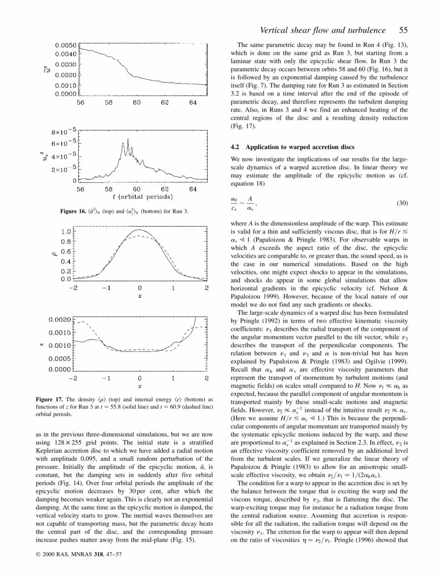
The same parametric decay may be found in Run 4 (Fig. 13),
which is done on the same grid as Run 3, but starting from a
laminar state with only the epicyclic shear flow. In Run 3 the
parametric decay occurs between orbits 58 and 60 (Fig. 16), but it
is followed by an exponential damping caused by the turbulence
itself (Fig. 7). The damping rate for Run 3 as estimated in Section
3.2 is based on a time interval after the end of the episode of
parametric decay, and therefore represents the turbulent damping
rate. Also, in Runs 3 and 4 we find an enhanced heating of the
central regions of the disc and a resulting density reduction
(Fig. 17).
4.2 Application to warped accretion discs
We now investigate the implications of our results for the large-
scale dynamics of a warped accretion disc. In linear theory we
may estimate the amplitude of the epicyclic motion as (cf.
equation 18)
u0
cs,
A
av
; �30�
where A is the dimensionless amplitude of the warp. This estimate
is valid for a thin and sufficiently viscous disc, that is for H=r &av ! 1 (Papaloizou & Pringle 1983). For observable warps in
which A exceeds the aspect ratio of the disc, the epicyclic
velocities are comparable to, or greater than, the sound speed, as is
the case in our numerical simulations. Based on the high
velocities, one might expect shocks to appear in the simulations,
and shocks do appear in some global simulations that allow
horizontal gradients in the epicyclic velocity (cf. Nelson &
Papaloizou 1999). However, because of the local nature of our
model we do not find any such gradients or shocks.
The large-scale dynamics of a warped disc has been formulated
by Pringle (1992) in terms of two effective kinematic viscosity
coefficients: n1 describes the radial transport of the component of
the angular momentum vector parallel to the tilt vector, while n2
describes the transport of the perpendicular components. The
relation between n1 and n2 and a is non-trivial but has been
explained by Papaloizou & Pringle (1983) and Ogilvie (1999).
Recall that ah and av are effective viscosity parameters that
represent the transport of momentum by turbulent motions (and
magnetic fields) on scales small compared to H. Now n1 / ah as
expected, because the parallel component of angular momentum is
transported mainly by these small-scale motions and magnetic
fields. However, n2 / a21v instead of the intuitive result n2 / av:
(Here we assume H=r & av ! 1:� This is because the perpendi-
cular components of angular momentum are transported mainly by
the systematic epicyclic motions induced by the warp, and these
are proportional to a21v as explained in Section 2.3. In effect, n2 is
an effective viscosity coefficient removed by an additional level
from the turbulent scales. If we generalize the linear theory of
Papaloizou & Pringle (1983) to allow for an anisotropic small-
scale effective viscosity, we obtain n2=n1 � 1=�2ahav�:The condition for a warp to appear in the accretion disc is set by
the balance between the torque that is exciting the warp and the
viscous torque, described by n2, that is flattening the disc. The
warp-exciting torque may for instance be a radiation torque from
the central radiation source. Assuming that accretion is respon-
sible for all the radiation, the radiation torque will depend on the
viscosity n1. The criterion for the warp to appear will then depend
on the ratio of viscosities h � n2=n1: Pringle (1996) showed that
Figure 16. kuÄ2lV (top) and ku2z lV (bottom) for Run 3.
Figure 17. The density kr l (top) and internal energy kel (bottom) as
functions of z for Run 3 at t � 55:8 (solid line) and t � 60:9 (dashed line)
orbital periods.
Vertical shear flow and turbulence 55
q 2000 RAS, MNRAS 318, 47±57

an irradiation-driven warp will appear at radii
r *2���
2p
ph
e
!2
RSch; �31�
where RSch is the Schwarzschild radius, and e � L= _Mc2 is the
efficiency of the accretion process. We have shown that ah <
av ! 1: However, we emphasize again that this does not imply
that h < 1; on the contrary, we estimate that h < 1=�2ahav� @ 1:The high value for h will make it difficult for a warp to appear
unless the radiation torque can be amplified by an additional
physical mechanism. One way to produce a stronger torque is if
the irradiation is driving an outflow from the disc (cf. Schandl &
Meyer 1994).
A similar damping mechanism may affect waves excited by
Lense±Thirring precession in the inner part of the accretion disc
around a spinning black hole. Numerical calculations by Markovic
& Lamb (1998) and Armitage & Natarajan (1999) show that these
waves are damped rapidly unless n2 ! n1; which we find is not thecase. (However, we note that the resonant enhancement of n2 will
be reduced near the innermost stable circular orbit, because the
epicyclic frequency deviates substantially from the orbital
frequency). Likewise a high value of n2 will lead to a rapid
alignment of the angular momentum vectors of a black hole and
its surrounding accretion disc (cf. Natarajan & Pringle 1998).
Some caution should be exercised when interpreting the results
of this paper. Although the shearing box simulations in general
have been successful in demonstrating the appearance of
turbulence with the right properties for driving accretion, they
are in general producing uncomfortably low values of ah to
describe, e.g., outbursting dwarf nova discs (see Cannizzo,
Wheeler & Polidan 1986). An underestimate of ah and av
would lead to an overestimate of h . In addition, the parametric
instability leads to an enhanced damping of the epicyclic motion.
If this effect had been sustained it would have resulted in a smaller
value for h. In a warped accretion disc, the epicyclic motion is
driven by the pressure gradients, which may maintain the
velocities at a sufficient level for the parametric instability to
operate continuously. To address this question we intend to study
forced oscillations in a future paper.
4.3 The vertical structure of the accretion disc
Our previous simulations of turbulence in a Keplerian shearing
box have shown that the turbulent xy stresses are approximately
constant with height (Brandenburg et al. 1996) rather than
proportional to the pressure as may have been expected from
the a -prescription (Shakura & Sunyaev 1973). We modified the
vertical boundary conditions for this paper and added an epicyclic
motion. However, the kBxByl stress is still approximately
independent of z or even increasing with |z| for jzj , H; whileat larger |z| we may see the effects of the boundary conditions
(Fig. 18). The effect of the epicyclic motion is seemingly to limit
the kBxByl stress in the surface layers to its value in the interior of
the disc. The fact that the stresses decrease more slowly with fzf
than does the density results in a strong heating of the surface
layers.
5 CONCLUSIONS
In this paper we have studied how the turbulence in an accretion
disc will damp an epicyclic motion, the amplitude of which
depends on the vertical coordinate z in the accretion disc. Such a
motion could be set up by a warp in the accretion disc (Papaloizou
& Pringle 1983). We find that the typical damping time-scale of
the epicyclic motion is about 25 orbital periods, which corre-
sponds to av � 0:006: This value is comparable to the traditional
estimate of ah that one gets from comparing the kruxuy 2 BxByl
stress with the pressure. Both alphas are of the order of 0.01,
which implies that the time-scale for damping a warp in the
accretion disc is much shorter than the usual viscous time-scale.
That the two alphas are within a factor of a few of each other is
surprising, since the damping of the epicyclic motion may be
attributed to the Reynolds stresses, while the accretion is mostly
driven by the Maxwell stress.
However, not all of the damping can be described as a simple
viscous damping. At high amplitudes the epicyclic motion may
also decay parametrically to inertial waves. The damping is much
more efficient in the presence of this mechanism.
ACKNOWLEDGMENTS
UT was supported by a European Union post-doctoral fellowship
in Cambridge and is supported by the Natural Sciences Research
Council (NFR) in Gothenburg. Computer resources from the
National Supercomputer Centre at LinkoÈping University are
gratefully acknowledged. GIO is supported by the European
Commission through the Training and Mobility of Researchers
network `Accretion on to Black Holes, Compact Stars and
Protostars' (contract number ERBFMRX-CT98-0195). This work
was supported in part by the Danish National Research Foundation
hrough its establishment of the Theoretical Astrophysics Center
(AÊ N). RFS is supported by NASA grant NAG5-4031.
REFERENCES
Armitage P. J., Natarajan P., 1999, ApJ, 525, 909
Balbus S. A., Hawley J. F., 1991, ApJ, 376, 214
Balbus S. A., Hawley J. F., 1998, Rev. Mod. Phys., 70, 1
Figure 18. The upper plot shows kB2l, the average of the magnetic energy,
as a function of z for Runs 3 at 66.3T0 (solid line) and 0 at 66.1T0 (dashed
line). The lower plot shows 2kBxByl plotted the same way.
56 U. Torkelsson et al.
q 2000 RAS, MNRAS 318, 47±57

Brandenburg A., 1999, in Abramowicz M. A., BjoÈrnsson G., Pringle J. E.,
eds, Theory of black hole accretion discs. Cambridge Univ, Press,
Cambridge, p. 61
Brandenburg A., Nordlund AÊ ., Stein R. F., Torkelsson U., 1995, ApJ, 446,
741
Brandenburg A., Nordlund AÊ ., Stein R. F., Torkelsson U., 1996, in Kato S.
et al., eds, Basic physics of accretion disks. Gordon & Breach, New
York, p. 285
Cannizzo J. K., Wheeler J. C., Polidan R. S., 1986, ApJ, 301, 634
Chandrasekhar S., 1960, Proc. Nat. Acad. Sci., 46, 253
Gammie C. F., Goodman J., Ogilvie G. I., 2000, MNRAS, in press (astro-
ph/0001539)
Hawley J. F., Gammie C. F., Balbus S. A., 1995, ApJ, 440, 742
Hawley J. F., Gammie C. F., Balbus S. A., 1996, ApJ, 464, 690
Katz J. I., 1973, Sci, 246, 87
Markovic D., Lamb F. K., 1998, ApJ, 507, 316
Matsumoto R., Tajima T., 1995, ApJ, 445, 767
Miyoshi M., Moran J., Herrnstein J., Greenhill L., Nakai N., Diamond P.,
Inoue M., 1995, Nat, 373, 127
Natarajan P., Pringle J. E., 1998, ApJ, 506, L97
Nelson R. P., Papaloizou J. C. B., 1999, MNRAS, 309, 929
Nordlund AÊ ., Stein R. F., 1990, Comput. Phys. Commun., 59, 119
Ogilvie G. I., 1999, MNRAS, 304, 557
Papaloizou J. C. B., Lin D. N. C., 1995, ApJ, 438, 841
Papaloizou J. C. B., Pringle J. E., 1983, MNRAS, 202, 1181
Pringle J. E., 1992, MNRAS, 258, 811
Pringle J. E., 1996, MNRAS, 281, 357
Roberts W. J., 1974, ApJ, 187, 575
Schandl S., Meyer F., 1994, A&A, 289, 149
Shakura N. I., Sunyaev R. A., 1973, A&A, 24, 337
Stone J. M., Hawley J. H., Gammie C. F., Balbus S. A., 1996, ApJ, 463,
656
Tananbaum H., Gursky H., Kellogg E. M., Levinson R., Schreier E.,
Giacconi R., 1972, ApJ, 174, L143
Terquem C. E. J. M. L. J., 1998, ApJ, 509, 819
Velikhov E. P., 1959, J. Exp. Theor. Phys., 9, 995 (Sov. Phys., 36, 1398 in
Russian original)
This paper has been typeset from a TEX/LATEX file prepared by the author.
Vertical shear flow and turbulence 57
q 2000 RAS, MNRAS 318, 47±57


